WORKING PAPER #47

Does the Market Value Value-Added? Evidence from Housing Prices After a Public Release of School and

Teacher Value-Added Scott Imberman

Michigan State University and NBER

Michael F. Lovenheim Cornell University and NBER

March 2015

The content of this paper does not necessarily reflect the views of The Education Policy Center or Michigan State University

Does the Market Value Value-Added? Evidence from Housing Prices After a Public Release of School and Teacher Value-Added

Author Information Scott Imberman Michigan State University and NBER Michael F. Lovenheim Cornell University and NBER

Acknowledgements We would like to thank seminar participants at the AEA Annual Meetings, the APPAM Fall Meetings, Case Western Reserve University, the CES-Ifo Economics of Education Meetings, Duke University, Georgetown University, the George Washington University, the NBER Economics of Education Meetings, the Society of Labor Economists Annual meeting, Texas A&M University, the University of Houston, the University of Illinois at Chicago, the University of Michigan, and the UM-MSU-UWO Labor Day Conference, along with John Bound, Julie Cullen, Steven Haider, Matt Hall, Susanna Loeb, Stephen Machin, Steven Rivkin, Guido Schwerdt, Gary Solon, and Kevin Stange for helpful comments and suggestions. We would also like to thank the Los Angeles County Tax Assessor’s Office, the Los Angeles Times, the Los Angeles Unified School District, and Richard Buddin for providing us the data and for their assistance with the data. Finally, we would like to thank Margaret O’Rourke, Michael Naretta and Leigh Wedenoja for excellent research assistance on this project. ⃝c 2015 by Scott Imberman and Michael Lovenheim. All errors and omissions are our own. Abstract

Value-added data have become an increasingly common evaluation tool for schools and teachers. Many school districts have begun to adopt these methods and have released results publicly. In this paper, we use the unique public release of value-added data in Los Angeles to identify how this measure of school quality is capitalized into housing prices. Via difference-in-differences, we find no evidence of a response to either school or teacher value-added rank, even though school-zone boundary fixed-effects estimates indicate that test score levels are capitalized into home prices. Given ample evidence that this information was new to residents, widely dispersed, and easily available, our results suggest that people did not significantly value it on the margin. This has implications for the effectiveness of providing value-added information as a tool to help parents choose schools.

Does the Market Value Value-Added?Evidence from Housing Prices After a PublicRelease of School and Teacher Value-Added

Scott A. Imberman∗

Michigan State University and NBER

Michael F. LovenheimCornell University and NBER

March, 2015

Abstract

Value-added data have become an increasingly common evaluation tool for schoolsand teachers. Many school districts have begun to adopt these methods and have releasedresults publicly. In this paper, we use the unique public release of value-added data inLos Angeles to identify how this measure of school quality is capitalized into housingprices. Via difference-in-differences, we find no evidence of a response to either schoolor teacher value-added rank, even though school-zone boundary fixed-effects estimatesindicate that test score levels are capitalized into home prices. Given ample evidence thatthis information was new to residents, widely dispersed, and easily available, our resultssuggest that people did not significantly value it on the margin. This has implicationsfor the effectiveness of providing value-added information as a tool to help parents chooseschools.

∗We would like to thank seminar participants at the AEA Annual Meetings, the APPAM Fall Meetings,Case Western Reserve University, the CES-Ifo Economics of Education Meetings, Duke University, GeorgetownUniversity, the George Washington University, the NBER Economics of Education Meetings, the Society ofLabor Economists Annual meeting, Texas A&M University, the University of Houston, the University of Illinoisat Chicago, the University of Michigan, and the UM-MSU-UWO Labor Day Conference, along with John Bound,Julie Cullen, Steven Haider, Matt Hall, Susanna Loeb, Stephen Machin, Steven Rivkin, Guido Schwerdt, GarySolon, and Kevin Stange for helpful comments and suggestions. We would also like to thank the Los AngelesCounty Tax Assessor’s Office, the Los Angeles Times, the Los Angeles Unified School District, and RichardBuddin for providing us the data and for their assistance with the data. Finally, we would like to thankMargaret O’Rourke, Michael Naretta and Leigh Wedenoja for excellent research assistance on this project.c⃝2015 by Scott Imberman and Michael Lovenheim. All errors and omissions are our own.

1 Introduction

Much prior research has been devoted to estimating the extent to which parents value the

quality of their local schools. Typically, the economics literature on school valuation uses the

capitalization of school quality measures into home prices to estimate the value local residents

place on school quality. The majority of school quality valuation studies use test score levels as

their measure of quality. Employing regression discontinuity methods at school attendance zone

boundaries, these studies tend to find that a one standard deviation difference in test scores is

associated with two to five percent higher property values (e.g., Bayer, Ferreira and McMillan,

2007; Kane, Riegg and Staiger, 2006; Black, 1999).1 Cross-school variation in test score levels

is driven by differences in the academic aptitude of the student body as well as the ability of

each school to produce student learning outcomes. Hence, it is not possible to separate out

parent valuation of high-achieving peers from parental valuation of the school’s ability to teach

students using these methods.

A few prior studies have attempted to overcome this problem by examining capitalization or

revealed preferences of parents based on “value-added” measures that seek to isolate the causal

effect of schools on student learning. The majority find no effect (e.g., Hastings, Kane and

Staiger, 2010; Brasington and Haurin, 2006; Dills, 2004; Downes and Zabel, 2002; Brasington,

1999), while Gibbons, Machin and Silva (2013) and Yinger (2014) show evidence that test

score levels and value-added are similarly valued. A central limitation to these studies is that

the value-added data are calculated by the researchers and likely are not known to parents.

However, in recent years, the push to expand test-based accountability has led to a marked

rise in the use and public release of school value-added estimates. This has been done in large

school districts in Los Angeles, Houston, and New York City, amongst others. The fact that

these data are increasingly prevalent and that controversy typically surrounds their release

underscores the importance of understanding how and whether parents value this information

when it is provided to them in a simplified manner.

In this paper, we provide what is to our knowledge the first evidence on how housing

1See Black and Machin (2011) and Nguyen-Huang and Yinger (2011) for comprehensive reviews of thisliterature.

1

markets respond to the public release of school and teacher value-added information. To do

this, we exploit a highly publicized, salient, and accessible data release in Los Angeles in 2010.

The information experiment that forms the basis for our study began in August 2010, when

the Los Angeles Times newspaper (LAT) published average value-added estimates for each

elementary school (470 in total) as well as individual value-added estimates for 6,000 third

through fifth grade teachers in the Los Angeles Unified School District (LAUSD). We show

that this value-added information was not predictable from existing information, nor was it

previously capitalized into home prices, suggesting that this was indeed new information for

local residents. The main focus of our analysis is on the short-run effect of this information on

property values, because in April 2011 LAUSD released its own value-added information and in

May 2011 the LA Times updated their value-added data to include more teachers. Prior work

has shown that home price responses to school quality information shocks occur quickly (Figlio

and Lucas, 2004; Fiva and Kirkebøen, 2011). This supports our focus on the seven-month time

period following the first value-added release that was free from influence from other value-

added information. Nonetheless, we also examine longer-run impacts (up to 13 months) after

the initial release, taking into account value-added rankings from all three releases to ensure

that our results are not simply due to the short time horizon.

Using home sales data we obtained from the Los Angeles County Assessor’s Office (LACAO)

from April 2009 through September 2011, we first show that test score levels are capitalized

at a rate similar to that found in the prior literature using school-zone boundary discontinuity

methods. We then estimate difference-in-differences models that identify how home prices

change after the release of value-added data as a function of the value-added scores. Despite

the strong valuation of test score levels and the fact that value-added rank largely was not

predictable from observable school characteristics prior to the release, we find no evidence

that school or teacher value-added information affects property values. Our estimates are

precise enough to rule out that learning one’s school is 10 percentiles higher in the value-added

distribution increases property values by more than 0.2 percent. This estimate indicates that a

one standard deviation increase in value-added (corresponding to about 35 percentiles in rank

at the median) would increase home prices by at most 0.7 percent, which is well below the

2

capitalization estimates of test scores levels in prior studies (Black and Machin, 2011).2 We

also show that the size of the information shock relative to existing information did not affect

property values.

Our empirical approach closely follows that of Figlio and Lucas (2004), who study the release

of “school report card” information in Florida as well that of Fiva and Kirkebøen (2011), who

examine the release of school ranking information in Oslo, Norway. Both of these papers find

that the new information on school quality had a large effect on property values but that the

capitalization effect dissipated within a year. Relative to this prior research, we make several

contributions to the literature. First, our study examines the effect of value-added measures of

school quality that can more credibly isolate the contribution of each school to student learning.

The school report cards studied by Figlio and Lucas (2004) are based on test score levels and

pass rates, which can differ substantially from value-added as they are much more strongly

correlated with school and neighborhood composition than with value-added. The information

examined by Fiva and Kirkebøen (2011) was based on student grade point averages (GPAs)

that were adjusted for student background characteristics. These estimates are closer to value-

added measures than are the school report cards in Figlio and Lucas (2004), but the lack of

lagged GPA controls makes it likely this information remains correlated with underlying student

quality differences across schools.3

Second, the estimates in Fiva and Kirkebøen (2011) are difficult to generalize to the US

context because of underlying differences in housing markets between Oslo and Los Angeles as

well as the fact that the 48 schools they study are, on average, high performing relative to the

rest of the country. The Los Angeles schools serve a much more diverse set of students and

include many low-performing schools in terms of test score levels. As we show below, many of

these low-test-score schools are actually calculated to be high value-added schools, which allows

us to disentangle parental valuation of test score levels from value-added in a setting with a

wide variance across schools in both measures.

2Our results also are consistent with evidence from Chile that signals of school quality beyond test scores donot affect enrollment patterns (Mizala and Urquiola, 2013).

3We also highlight that our approach differs from those who have used researcher-calculated value-added(e.g., Downes and Zabel, 2002) due to the fact that in our setup parents actually observe value-added.

3

Third, this paper is the first in the literature to examine how parents value direct measures of

teacher quality. Prior work has focused solely on school quality valuation, but the importance of

teachers has been overlooked. Because the LA Times released teacher value-added measures as

well as school measures, we can estimate how home prices respond to teacher quality, per se. The

LA Times teacher value-added model used in our context has been shown to exhibit little bias

(Guarino, Reckase and Wooldridge, 2015; Chetty, Friedman and Rockoff, 2014a; Kane et al.,

2013; Kane and Staiger, 2008) and appears to be a good measure of a teacher’s contribution to

long-run student outcomes, such as earnings and college-going (Chetty, Friedman and Rockoff,

2014b). That this value-added information is a strong measure of school and teacher quality

does not mean parents valued it as such, however; this study is the first to be able to examine

this question directly.4

Overall, our results indicate that releasing straightforward value-added rankings to the pub-

lic does not affect property values, which suggests that homeowners do not value the informa-

tion as currently constructed on the margin. The lack of responsiveness to this information

either could be driven by parents placing little value on the ability of schools and teachers to

increase test scores or by parents and homeowners ignoring value-added information because

its release was highly contentious and the measures are derived from a complicated statistical

model that is opaque to non-experts. We argue the preponderance of the evidence is consistent

with the former mechanism, because the information was presented in a simple-to-understand

manner by a highly-respected and impartial newspaper, the release was highly publicised and

salient, and there was no response to the release of a separate value-added measure by LAUSD

which parents may have trusted more because it came directly from the schools. Indeed, this

finding is consistent with the fact that boundary-discontinuity estimates of school quality are

reduced significantly once neighborhood characteristics are controlled for (Bayer, Ferreira and

McMillan, 2007; Kane, Riegg and Staiger, 2006) as well as the fact that most prior research

has not found an effect of researcher-calculated value-added on property values. Rothstein

(2006) also provides indirect evidence that parents do not highly value the ability of schools

4Jacob and Lefgren (2007) show that within schools, parents have a revealed preference for teachers that arebetter at raising student test scores. But, parent information on teacher quality in that study does not comefrom value-added measures.

4

to raise test scores, as observed residential sorting is inconsistent with these preferences. This

paper provides a more direct test of this question than has been possible in prior studies, but

our results are consistent with much of the existing research in this area. Thus, our results

provide new information about valuation of a school quality measure that provides previously

unknown information about a school’s or teacher’s contribution to test score growth rather than

information about the demographic makeup of the school.

2 The Release of Value-Added Information in Los An-

geles

In 2010, the Los Angeles Times newspaper acquired individual testing records of elementary

students in Los Angeles Unified School District via a public information request. The achieve-

ment scores were linked to teachers so that a teacher and school value-added analysis could

be conducted. The LA Times hired Dr. Richard Buddin to conduct the statistical analysis.

Details on the methodology can be found in Buddin (2010), but the basic strategy is to use a

linear regression model with teacher fixed effects to calculate teacher value-added. Teacher fixed

effects are replaced with school fixed effects to calculate school value-added. All models use

data from the 2002-2003 through the 2008-2009 school years and control for lagged test scores

and student characteristics. The use of several years of data has the benefit of increasing the

precision of the value-added estimates relative to using only one year of recent data. Following

completion of the analysis, the newspaper wrote a series of articles explaining the methodology

and other issues in LAUSD throughout the month of August 2010 as a lead in to the release

of the data in a simplified form on August 26, 2010. The value-added data were presented

through an online database and could be accessed by anyone with a computer without charge

or registration.5 The database was searchable by school and teacher name, and people also

could access information through various links off of the main web page.

5The current version of the database can be accessed at http://projects.latimes.com/value-added/. The webportal is similar to the one that was available in August 2010 but now provides information for more teachersand more details on the value-added measures. In most cases, one can access the original August 2010 releasethrough links on the teacher and school web pages.

5

Figure 1 shows an example of how the information was presented for a given school. Schools

were categorized as “least effective,” “less effective,” “average,” “more effective,” and “most ef-

fective,” which refer to the quintiles of the value-added score distribution for LAUSD. However,

as Figure 1 demonstrates, the black diamond shows each school’s exact location in the distri-

bution, providing parents with the ability to easily estimate the school’s percentile. Although

value-added scores were generated separately for math and reading, the LA Times based their

categorization on the mean of the two scores. The figure also shows the location of the school’s

Academic Performance Index (API) percentile. API is an summary measure provided by the

state of California that measures school quality via a weighted average primarily composed of

test scores along with some other outputs such as attendance. Although the API information

was publicly available prior to August 2010, it was more difficult to find and was not accom-

panied by the heightened media attention that accompanied the value-added release. Thus,

for many people, this API information could have been new. The value-added rank was not

available in any form prior to August 2010. Finally, the web page provides passing rates on

the math and English exams for each school, which was also publicly available prior to the

value-added release. To keep our estimating equation simple, in our analyses we will assume

that any response to the LA Times reprinting the passing rates will be reflected in responses

to API.6

A critical question underlying our analysis is whether LA residents knew about the release

of this information. Note that any school quality information intervention carries with it the

difficulty of ensuring that those who are targeted receive the information. We believe the

structure of this information release, with the information being available online for free and

the publicity that surrounded its release, made the value-added information more salient than

is typical with school quality information releases.7 Indeed, there is substantial evidence to

indicate that residents were well-informed about the LA Times database. First, the Los Angeles

6This assumption is sensible because API scores are calculated almost entirely by using scores on theseexams.

7Due to the prevalence of the Internet in 2010, the penetration of this information in Los Angeles likelywas at least as large as in Florida when they first released school report card information in the late 1990s.Figlio and Lucas (2004) show that the Florida information release, which was less contentious, had less publicitysurrounding it, and occurred in a period in which information was more difficult to obtain, had large effects onproperty values.

6

Times is the largest newspaper in Southern California and the fourth largest in the country by

daily weekday circulation, with 616,575 copies according to the Audit Bureau of Circulations.

The existence of the database was widely reported in the newspaper: from August 2010 to May

2011, a total of 37 articles or editorials were written about the database, public response to the

database, or value-added issues more generally. Given the high level of circulation of the paper,

the attention paid to this issue by the LA Times likely reached many residents. Further, the

release of the value-added data was mentioned in other outlets, such as the New York Times,

National Public Radio, the Washington Post, ABC News, CBS News, CNN and Fox News. It

also received much radio and television attention in the LA area in both English and Spanish,

which is of particular importance for the Spanish-speaking population that is less likely to read

the LA Times but for whom radio and television are dominant sources of news.8

Second, the LAUSD teachers’ union and the national American Federation of Teachers were

highly vocal in their opposition to the public release of the data. This culminated in a series

of highly publicized and widely covered protests of the LA Times by teachers. In addition,

US Secretary of Education Arne Duncan spoke about the value-added measures, expressing

his support. This indicates that news-makers were discussing the issue and gave it substantial

media exposure. According to the LA Times, by late afternoon on the initial date of the

release there were over 230,000 page views of the website for the database (Song, 2010). The

article points out that this is an unusually large volume of views given that traffic tends to

be higher during the week and provides prima facia evidence that the value-added release was

well-publicized and known to a large number of residents. In part due to its contentious nature

as well as the involvement of the largest newspaper in the area, it is unlikely there could be a

school quality information intervention in which the information was more readily available to

local residents than was the case here.

A related issue is whether most parents were able to access the data. Given the low income

of many families with children in LAUSD and the fact that there was no print release of the

8Some examples of Spanish language coverage include a story on Channel 22 on Nov. 8,2010 covering a protest after a teacher committed suicide in part due to value-added results(http://www.youtube.com/watch?v=RWKR8Ch06wY), a story covering an earlier protest on Channel 62(http://www.youtube.com/watch?v=n1iNXtyPlRk), and a story on Univision 34 discussing LAUSD’s ownvalue-added measures (http://www.youtube.com/watch?v=05dE0xLdpu8).

7

value-added scores (they were only provided online), this is not obvious. To check this we use

data from the October 2010 Current Population Survey supplement on computer and Internet

usage. While the sample size is small (295 observations), 87% of adults in Los Angeles age 25 or

older and who never attended college had Internet access at home. Using the far larger sample

of all Californians 25 or older who never attended college (2,156 observations), 91% have access

to the Internet at home. These data indicate that the residents of Los Angeles who ought to

have the largest interest in the value-added scores were able to access them.

The 2010 LA Times value-added information is the focus of our analysis. This focus neces-

sitates an examination of short-run impacts on property values because this initial value-added

data release was followed up with LAUSD releasing its own school-level value-added measure in

April 2011 and the LA Times updating its value-added measure in May 2011.9 While examining

the effect of the initial LA Times release provides a purer information experiment, it limits the

analysis to 7 months post-release. Even so, in their analysis of the capitalization of value-added

information in Norway, Fiva and Kirkebøen (2011) show that the positive effects were very

short-run, on the order of 3 months. Figlio and Lucas (2004) further show evidence that the

positive impact of school report card information in Florida on property values were largest in

the first year post-release. This evidence supports our examination of short-run effects.

We also analyze longer-run effects that account for the subsequent value-added releases.

Thus, it is important to highlight several differences between the first LA Times release and

subsequent data releases. First, we believe the LA Times used a more econometrically sound

value-added model than LAUSD, as the former model controls for lagged achievement and

includes multiple years of data. Guarino, Reckase and Wooldridge (2015) argue that models like

this (which they call “dynamic ordinary least squares”) are the most accurate.10 The LAUSD

model, on the other hand, predicts student achievement growth from observable characteristics

9LAUSD’s value-added measure was called Achievement Growth over Time (AGT) and was onlyprovided to the public at the school level. The details of their methodology can be found athttp://portal.battelleforkids.org/BFK/LAUSD/FAQ.html. Details on the May 2011 LA Times methodologycan be found in Buddin (2011). For this release, the LA Times also gave people the option to see how value-added scores changed using variations in methodology through an interactive program on the website. Since itis likely that most people who accessed the database did not attempt to compare different methods, we onlyuse the value-added scores directly published on the website by the LA Times in our data.

10The May 2011 LA Times release updated this model to include an extra year of data, more teachers andapplied Bayesian shrinkage adjustments as in Kane and Staiger (2008) to the estimates.

8

using one year of data, after which the differences between predicted and actual achievement

are averaged together across all students in a school. While the LA Times methodology may

be more appealing to researchers, we acknowledge that this does not necessarily indicate that

parents believed it more. Second, there was substantial discussion of the intial LA Times release

in the news and responses by education organizations, while the subsequent releases garnered

less attention. Finally, it is easier to access the LA Times information. While both are available

on the web, to access the LAUSD data people need to navigate through a series of links on the

LAUSD website.

It also is interesting to note that the correlations between both of the LA Times releases

and the LAUSD value-added scores are very low. Figure 2 presents comparisons of the three

school-level value-added measures using scatter plots with each school as an observation. The

top left panel shows that the percentiles of the 2010 LA Times value-added are highly correlated

with the 2011 LA Times value-added, with a correlation coefficient of 0.74.11 However, each of

the LA Times value-added measures are very weakly correlated with the LAUSD measure - the

correlation coefficients are 0.15 and 0.39 for the August and May releases, respectively. This

likely reflects the differences in the methodology described above and the amount of data used.

3 Data

To assess the impact of the value-added data release on property values, we combine data from

several sources. First, we use home price sales data from the Los Angeles County Assessor’s

Office (LACAO). The data contain the most recent sale price of most homes in LA County

as of October, 2011, which in addition to LAUSD encompasses 75 other school districts. We

restrict our data to include all residential sales in LAUSD that occurred between April 1, 2009

and September 30, 2011.12 From LACAO, we also obtained parcel-specific property maps,

11An important question arises as to why the value-added estimates differed across LA Times data releases.This was due to three factors: methodology changes, increases in the number of teachers included in the value-added calculations, and an additional year of data on teachers included in the first release. If we drop all schoolswith percentile rank changes greater than 20, the correlation between value-added ranks across LAT releasesis 0.96. Critically, our estimates are unaffected by this sample restriction. These results are available uponrequest.

12Given that the value-added information only varies across schools within LAUSD, the addition of schoolfixed effects leaves little to be gained from adding the rest of LA County. Specifications using home price salesfrom all of the county, setting value-added percentiles equal to zero outside of LAUSD and controlling for school

9

which we overlay with the school zone maps provided to us by LAUSD to link properties to

school zones.13 Although there is open enrollment throughout LAUSD, spaces are very limited

at around 1.5% of total enrollment. Thus, these catchment zones define the relevant school

for the vast majority of students in the District. The property sales data additionally contain

information on the dates of the three most recent sales, the square footage of the house, the

number of bedrooms and bathrooms, the number of units and the age of the house that we will

use to control for any potential changes in the composition of sales that are correlated with

value-added information.

To remove outliers, we drop all properties with sale prices above $1.5 million (5% of house-

holds) and limit our sample to properties in elementary school zones in Los Angeles Unified

School District that received value-added scores in the August 2010 release. About 25% of the

residential properties in the data do not have a sale price listed. Usually, these are property

transfers between relatives or inheritances.14 Hence, we limit our sample to those sales that

have “document reason code” of “A,” which denotes that it is a “good transfer” of property.

After making this restriction, only 7% of observations are missing sale prices. For these ob-

servations, we impute sale prices using the combined assessed land and improvement values of

the property.15 For observations that have all three measures recorded, the correlation between

actual sale price and the imputed sale price is 0.89, indicating that the imputation is a very

close approximation to the actual market value. Furthermore, we know of no reason why the

accuracy of the imputation procedure should be correlated with value-added information, which

supports the validity of this method. Nonetheless, in Section 5, we provide results without im-

puted values and show they are very similar. Our final analysis data set contains 63,122 sales,

district fixed effects, provide almost identical results.13The school zones are for the 2011-2012 school year.14California allows relatives to transfer property to each other without a reassessment of the home’s value for

property tax purposes. Due to property tax caps, this rule creates large incentives for within-family propertytransfers in California, and hence there are a lot of such transactions in the data. Because these transfers donot reflect market prices, we do not include them in our analysis.

15Rather than impute the values one could simply drop the observations with missing sale price. However, todo this one would have to assume that sale prices are missing at random, at least conditional on controls. InOnline Appendix Table A-1 we estimate models that look at correlations between property characteristics andwhether the sale price is missing. Even when controlling for school and time fixed effects we find a substantialnumber of characteristics are significantly correlated with a property missing the sale price. This suggests theobservations are unlikely to be missing at random.

10

51,514 of which occur prior to April 2011.

We obtained the exact value-added score for each school directly from Richard Buddin, and

the April 2011 LA Times school value-added data as well as the August 2010 teacher-level value-

added data were provided to us by the LA Times. The LAUSD value-added information was

collected directly from Battelle for Kids, with whom LAUSD partnered to generate the value-

added measures.16 The value-added data were combined with school-by-academic-year data on

overall API scores, API scores by ethnic and racial groups, school-average racial composition,

percent on free and reduced price lunch, percent disabled, percent gifted and talented, average

parental education levels, and enrollment. These covariates, which are available through the

California Department of Education, control for possible correlations between value-added in-

formation and underlying demographic trends in each school. To maintain consistency with the

LA Times value-added data, we convert both the LAUSD value-added scores and API scores

into percentile rankings within LAUSD.

Similar to Black (1999), we also link each property to its Census block group characteristics

from the 2007-2011 American Communities Survey (ACS) to use as controls. In particular,

we use the age distribution of each block group (in 5 year intervals), the percentage with each

educational attainment level (less than high school, high school diploma, some college, BA or

more), the percentage of female headed households with children, and median income. We also

collect a host of additional Census tract level data from the 2007-2011 ACS. These are used to

help test the validity of our identifying assumptions.

Summary statistics of some key analysis variables are shown in Table 1. The table presents

means and standard deviations for the full sample as well as for the sample above and below

the median value-added score for the 2010 LA Times release. On average, home sales in

LAUSD are in Census block groups that are over 50% black and Hispanic,17 but the schools

these properties are zoned to are 74% black and Hispanic, with the difference ostensibly due

to enrollments in private, charter and magnet schools. The schools in our data set also have a

large proportion of free and reduced price lunch students. The second two columns of Table 1

16The data are available at http://portal.battelleforkids.org/BFK/LAUSD/Home.html.17Note that since the ACS counts Hispanic as a separate category from race, some of the black and white

populations are also counted as Hispanic.

11

show that value-added is not completely uncorrelated with school or block group demographics,

although housing characteristics are balanced across columns. The higher value-added areas

have a lower minority share, higher property values, a more educated populace and have higher

API scores. These correlations likely are driven by better schools being located in the higher

socioeconomic areas.

Figure 3 shows that, despite the differences shown in Table 1, value-added is far less cor-

related with student demographic makeup than are API scores. The figure presents the non-

free/reduced-price (FRP) lunch rate, API percentile (within LAUSD) and value-added per-

centile for each elementary school in LAUSD. The boundaries denote the attendance zone for

each school. As expected, API percentiles, which are based on test score proficiency rates,

map closely to poverty rates. High-poverty (low non-FRP lunch) schools tend to have lower

API scores. While this relationship remains when replacing API with value-added, it is far

less robust. There are many schools, particularly in the eastern and northern sections of the

district, where API scores are low but value-added scores are high. Similarly, some schools with

high API scores have low value-added scores. Figure 4 further illustrates this point. It provides

scatter plots of API percentiles versus value-added percentiles for each of the three value-added

measures. While there is a positive relationship between value-added and test score levels, it

is quite weak: the correlation between the 2010 LAT value-added rank and API rank is only

0.45. As seen in Figure 3, there are a number of schools which, based on API, are at the top of

the distribution but according to the value-added measure are at the bottom, and vice-versa.

For example, Wilbur Avenue Elementary had an API percentile of 91 in 2009 but an initial

value-added percentile of 13. On the other end of the spectrum, Broadous Elementary had an

API percentile of 5 but a value-added percentile of 97.

The fact the API rank and value-added rank are only weakly related to each other does

not mean that the value-added information provided by the LA Times was new information.

It is possible that each of these measures could be predicted based on existing observable

characteristics of the school. In Table 2, we examine this issue directly, by predicting API

percentile and the percentiles of each value-added measure as a function of school observables in

the pre-release period. We use as our predictors of school quality all of the school-level variables

12

included in our property value analysis in order to show how much unexplained variation

there is in value-added rank after controlling for school characteristics included in our main

empirical model. Column (1) shows the results for API percentile, and as expected, with an

R2 of 0.71, school demographics explain a substantial amount of the variation. In contrast, as

shown in column (2), the value-added estimates are much more weakly correlated with school

demographics. Only two of the estimates are statistically significant at the 5% level, and the

R2 is only 0.22. In Column (3), we add overall API, within-LAUSD API rank, and each student

subgroup’s API scores as well as two years of lags of each of the API scores as regressors. The R2

rises but remains low, at 0.41. Thus, almost 60% of the value-added variation is unpredictable

from the observable characteristics of the school, including test score levels. In the final four

columns, we show results from similar models that use the percentiles in the second LAT value-

added release (columns 4 and 5) and the LAUSD value-added release (columns 6 and 7) as

dependent variables. The results are similar to those using the first LAT release.

Table 2 and Figures 3-4 show that the value-added data released to the public by the LA

Times and LAUSD contained new and unique information about school quality that was not

predictable from observed demographics and school test score levels. Our empirical model

exploits this new information by identifying the impact of value-added on housing prices condi-

tional on API along with many other observable characteristics of schools and neighborhoods.

Since these characteristics are observable to homeowners as well, we are able to identify the

impact of this new information given the information set that already exists.

4 Valuation of Existing School Quality Information

Before discussing the impacts of the value-added release, it is useful to to establish that some

measures of school quality are indeed valued by LA residents. Whether public school quality,

or public school characteristics more generally, are capitalized into home prices in Los Angeles

is not obvious, as LAUSD has a school choice system in which students can enroll in a non-

neighborhood school if space is available. There also is a large charter school and private school

presence in the district. Thus, any finding that property values do not respond to value-added

13

information could be driven by a general lack of association between local school characteristics

and property values. Nonetheless, there are a few reasons to believe that this is not a major

concern in the Los Angeles context. First of all, the open-enrollment program is small relative to

the size of the district. In 2010-2011, only 9,500 seats were available district-wide, accounting for

at most 1.5% of the district’s 671,000 students. Second, while LAUSD has a number of magnet

programs, they are highly sought after and oversubscribed, hence admission to a desired magnet

is far from guaranteed. Third, Los Angeles is a very large city with notorious traffic problems

and poor public transportation, making it difficult for parents to send their children to schools

any substantial distance from home.

To further address this issue, we estimate boundary fixed effects models in which API

percentile is the key independent variable. This model is similar to the one used in Black

(1999) as well as in the subsequent other boundary fixed effects analyses in the literature

(Black and Machin, 2011) and allows us to establish whether average test scores are valued in

LA as they have been shown to be in other areas. We estimate boundary fixed effects models

using only data from prior to the first release of the LA Times value-added data so that none

of these estimates can be affected by this information.18

Panel A of Table 3 contains results comparing home prices within 0.2 miles of an elementary

attendance zone boundary. In column (1), which includes no controls other than boundary

fixed-effects, properties just over the border from a school with a higher API rank are worth

substantially more. For ease of exposition, all estimates are multiplied by 100, so a 10 percentage

point increase in API rank is associated with a 4.5% increase in home values in the pre-release

period. In column (2), we control for housing characteristics, which have little impact on the

estimates. However, controlling for Census block group demographics in column (3) significantly

reduces this association. This result is not surprising given the findings in Bayer, Ferreira and

McMillan (2007) and Kane, Riegg and Staiger (2006).19 Nonetheless, in column (3), we find a 10

percentage point increase in API rank is correlated with a statistically significant 1.3% increase

18More precisely, we estimate Yistb = γ0+ γ1APIst+HiΩ+υt+ ζsi,sk +µistb, where Y is log sales price, H isthe set of Census block and property characteristics described above, υt is a set of month-by-year fixed effectsand ζsi,sk is a set of attendance zone boundary fixed effects for each contiguous school pair i and k.

19We do not control for school demographics because these demographics may be part of what determinesthe valuation of API.

14

in property values. This estimate is roughly equivalent in magnitude to those in Black (1999)

and Bayer, Ferreira and McMillan (2007). Thus, this school characteristic is similarly valued in

Los Angeles as in the areas studied in these previous analyses (Massachusetts and San Francisco,

respectively). Estimates using properties within 0.1 mile of a school zone boundary are similar,

as shown in Panel B.20 It remains unclear, however, whether the capitalization of API scores

is driven by valuation of schools’ contribution to learning or by valuation of neighborhood or

school composition that is correlated with API levels. Our analysis of capitalization of value-

added information is designed to provide insight into resolving this question, which is very

difficult to do without a school quality measure that is only weakly correlated with student

demographics.

In order to underscore the fact that, conditional on achievement levels, value-added is weakly

correlated with student demographics and is difficult to predict with pre-release observables,

the final column of Table 3 tests whether value-added information is capitalized into property

values prior to the public release. If parents know which schools are the highest value-added

from reputation or from factors we cannot observe, the value-added release should not provide

additional information about school quality and should already be capitalized into home prices.

In column (4) of Table 3, we estimate the same boundary fixed effects model as in column (3)

but include the first LA Times VA percentile as well. The estimate, based off of data in the

pre-release period, tests whether future information about value-added is already capitalized

into home prices. The results show that in the pre-release period, property values were not

significantly higher right across a school catchment boundary when future value-added is higher.

The estimate is small and is not statistically significant at conventional levels regardless of

whether we limit to 0.2 or 0.1 miles from the boundary. However, the API boundary effect

is very similar to the estimate in column (3), suggesting that the capitalization of API scores

is not being driven by value-added information and that any information contained in the LA

Times value-added estimate is not already capitalized into home prices prior to August 2010.

Overall, we view the results in Table 3 as showing that the value-added information released

20The 0.2 and 0.1 bandwidths were chosen to be consistent with prior work, most notably Black (1999) andBayer, Ferreira and McMillan (2007).

15

through the LA Times website was not previously known to residents.

5 Empirical Strategy

Our main empirical strategy to identify the effect of value-added information on property values

is to estimate difference-in-difference models that compare changes in property values surround-

ing the information releases as a function of value-added rank conditional on observable school

and neighborhood characteristics, including API. Since value-added only was released for ele-

mentary schools, we ignore middle and high school zones. Our main empirical model is of the

following form:

Yist = β0 + β1V Ast + β2APIst + β3APIst × Postt

+XstΓ +HiΦ + λt + γs + ϵist, (1)

where Yist is the log sale price of property i in elementary school zone s in month t. The

key explanatory variable of interest is V Ast, which is the August 2010 LA Times value-added

percentile. This variable is set equal to zero prior to the first release in September, 2010 and is

equal to the LA Times value-added percentile rank thereafter. In order to focus on the first LA

Times information shock, we estimate this model using data from April 1, 2009 to March 31,

2011. This sample restriction allows for 7 months of property sale observations post-treatment.

As discussed in Section 2, the LA Times also posted API rank on their website, which

may have made this information more salient to residents. Thus, in equation (1) we allow

for the effect of API to vary post-August 2010. Furthermore, we include in the model school

fixed effects (γs) that control for any fixed differences across schools that reflect fixed school

quality differences and month-by-year fixed effects (λt) that control for any district-level changes

in home prices occurring contemporaneously with the information release, including seasonal

changes. Our inclusion of these fixed effects implies that all parameters are identified off of

within-school changes in home prices over time. The coefficients β1 and β3 thus represent

difference-in-difference estimates of the effect of having a higher value-added or API score on

16

property values after the information release relative to before the release.21 In order to account

for the fact that there are multiple sales per school zone, all estimates are accompanied by robust

standard errors that are clustered at the school-zone level.

Equation (1) also includes an extensive set of controls to account for any confounding

effects driven by the correlation between the value-added release and contemporaneous changes

in school demographics or housing characteristics. The controls further allow us to condition as

best we can on the existing information set. The vector X contains the set of school observables

discussed above, including current and two years of lagged overall API, current and two years

of lagged API for each student subgroup,22 within-LAUSD API percentile rank in the given

academic year,23 the percent of students who are black, Hispanic, and Asian, the percent on

free/reduced price lunch, who are gifted, who are in special education and who are English

language learners. School-by-year enrollment and the percent of the school’s parents who are

high school graduates, have some college, have a BA and have graduate school training are

included in X as well. The vector H is the set of house-specific characteristics and Census

block group characteristics discussed above that further control for local demographic differences

that are correlated with value-added and for any changes in the types of houses being sold as

a function of value-added when the information is released.

There are two main assumptions underlying identification of β1 in equation (1). First, the

model assumes that home prices were not trending differentially by value-added prior to the data

release. Using the panel nature of our data, we can test for such differential trends directly in

an event-study framework. In Figure 5, we present estimates using the first value-added release,

where V A and API are interacted with a series of indicator variables for time relative to the

August 2010 LA Times release.24 These estimates stop at 7 months post-treatment due to the

subsequent data releases. The top panel of Figure 5 shows no evidence of a pre-release trend in

21Note that unlike API, which changes each year, each value-added release provides a single value for eachschool, and thus the main effect is removed by the school fixed effects. In models that do not include schoolfixed effects, the main effect is included as a control variable.

22Student subgroups include blacks, whites, Asians, Filipinos, Hispanics, gifted students, special education,economically disadvantaged and English language learners.

23For this study we define the academic year as running from September through August.24Event studies using the full analysis period and including all three VA releases are provided in Online

Appendix Figure 1.

17

home prices as a function of LAT value-added. The estimates exhibit a fair amount of noise,

but home prices are relatively flat as a function of future value-added rank in the pre-treatment

period. Thus, there is no evidence of pre-treatment trends that would bias our estimates. For

API shown in the bottom panel, there is a slight downward trend in earlier months, but it is

not statistically different from zero. By 7 months prior to the release, however, property values

flatten as a function of API.

Figure 5 also previews the main empirical finding of this analysis: home prices do not change

as a function of value-added or API post-release. The figure shows as well that these estimates

are relatively imprecise, as event study models are demanding of the data. We thus favor the

more parametric model given by equation (1). Nonetheless, Figure 5 demonstrates that there

do not appear to be any time-varying treatment effects that are masked by the equation (1)

specification.

The second main identification assumption required by equation (1) is that the value-added

percentile, conditional on school characteristics, is not correlated with unobserved character-

istics of households that could affect prices. While this assumption is difficult to test, given

the rich set of observable information we have about the homes sold, examining how these

observables shift as a function of value-added will provide some insight into the veracity of this

assumption. Thus, in Table 4, we show estimates in which we use neighborhood characteristics

(measured using both Census block group and Census tract characteristics), school demograph-

ics and housing characteristics as dependent variables in regressions akin to equation (1) but

only including API percentiles, API percentile interacted with a post-release indicator, time

fixed effects and school fixed effects as controls.25 Each cell in the table comes from a separate

regression and shows how the observable characteristic changes as a function of value-added

percentile after the first LA Times data release. Overall, the results in Table 4 provide little

support for any demographic or housing type changes that could seriously impact our estimates.

There are 53 estimates of housing and neighborhood characteristics in the table; two are sig-

nificantly different from zero at the 5% level and only 5 (including the two just mentioned) are

significant at the 10% level. While clearly these variables are not independent, if they were we

25The school characteristics estimates in Panel C use data aggregated to the school-year level.

18

would expect to falsely reject the null at the 10% level five times.26 Furthermore, the estimates,

even when significant, are small, and the signs of the estimates do not suggest any particular

patterns that could cause a systematic bias in either direction.

Another concern is that the release of a value-added score may induce changes in the number

of homes sold in a school catchment area. Since we only observe prices of homes that are sold,

we may understate the magnitude of the effect if having a lower value-added reduces the number

of homes sold and this reduction comes from the bottom of the price distribution. To test this

hypothesis, we estimate a version of equation (1) in which we aggregate the data to the school-

month level and use the total number of sales or the total number of sales with a valid sales

price in each school-month as the dependent variable.27 We find little evidence of a change

in the number of sales. The estimate of the effect of LA Times value-added on total sales28

is -0.0098 with a standard error of 0.0062. Taken at face value, this would suggest that a 10

percentile increase in value-added only reduces monthly sales by 0.1 off of a mean of 8.4. For

sales with price data, the estimate is -0.0027 with a standard error of 0.0032.

The value-added releases we study come at a time of high volatility in the housing market,

though, as we describe below, our analysis begins after prices in Los Angeles had stabilized.

Even so, this was a period with a large number of foreclosures in Los Angeles. If foreclosure rates

are correlated with the value-added releases, it could bias our home price estimates because

foreclosures tend to be sold at below market value. In order to provide some evidence on this

potential source of bias, we use the number of foreclosures in each month and zip code in LAUSD

that were collected by the RAND Corporation.29 We aggregate prices to the school-month

level and use the zipcode-level data to approximate the number of foreclosures in the school

catchment area in each month. The resulting estimates show little evidence of a correlation

between value-added post-release and the number of foreclosures. The coefficient on the LA

26Estimates that include the second LA Times release and the LAUSD data also show no evidence that therelease of these data is correlated with demographic changes in schools or neighborhoods. These results areavailable upon request.

27We include neighborhood characteristics of properties sold in a school zone and school characteristics butdo not control for aggregate individual property characteristics as these may be endogenous in this regression.

28Our data only cover the three most recent sales of a property. Thus, our measure of total sales will beslightly underestimated.

29These data are available at http://ca.rand.org/stats/economics/foreclose.html.

19

Times value-added variable is only 0.003 (0.009), which indicates that a 10 percentile value-

added rank increase post-release increases the number of monthly foreclosures in a school zone

by 0.03, off of a mean of 5.7. Overall, the estimates described above along with those provided

in Table 3 and Figure 5 provide support for our identification strategy.

Equation (1) includes only 7 months of post-release property sales. In order to examine

longer-run effects, we modify the estimating equation to account for the subsequent releases of

value-added information by the LA Times and by LAUSD. The model we estimate is:

Yist = β0 + β1V ALAT1st + β2V ALAT2

st + β3V ALAUSDst + β4APIst + β4APIst × Postt

+XstΓ +HiΦ + λt + γs + ϵist, (2)

where V ALAT1st is the first LA Times value-added measures, which is equal to zero prior to the

first release in September, 2010. The variable V ALAT2st is the second LA Times value-added

measure and is equal to zero prior to May 2011, and V ALAUSDst is the LAUSD value-added

measure, which is set equal to zero prior to April 2011. All other variables are as defined above.

In addition to models (1) and (2), we extend the boundary fixed-effect analysis in Table 3

to the difference-in-differences context. If one is concerned that our identification assumptions

do not hold in general, they are much more likely to hold when we compare changes in housing

prices generated by the value-added release to households on either side of an elementary

school zone boundary. For these models, we restrict to properties within 0.1 mile of a school

zone boundary and estimate (for the 7 month sample)

Yist = β0 + β1V ALAT1st + β2APIst + β3APIst × Postt

+XstΓ +HiΦ + λt + γs + ζsi,sk + ϵist, (3)

where ζsi,sk is an indicator that equals one if the property is on the boundary between school

i and school k. We also extend equation (2) in a similar manner to equation (3) for the

longer-term sample.

20

6 Results

6.1 Difference-in-Difference Estimates

Table 5 presents the baseline estimates from equation (1). In each column, we add controls

sequentially in order to observe the effects of the controls on the estimates. All estimates

are multiplied by 100, so they show the effect of a 100 percentile increase in value-added on

home prices post-release. Panel A shows results examining just the first LA Times value-added

information. We include no controls except API and VA main effects in column (1) and then

add in the school, neighborhood and housing characteristics discussed in Sections 3 and 5 in

column (2). Column (3) contains our preferred estimates, which include school zone and month

fixed effects. Across columns, there is no evidence that a higher value-added rank leads to higher

home prices. Regardless of the controls used, the estimates are small and are not statistically

significant. In column (3), the point estimates indicate that a 10 percentile point increase in

value-added decreases property values by 0.3 percent. This estimate is precise enough that we

can rule out a 10 percentile point increase in value-added increases home prices by more than

0.2% post-release. To relate this estimate to the prior literature, at the median a one standard

deviation increase in value-added corresponds to a roughly 35 percentile increase in rank. Using

the upper bound of the 95% confidence interval, this translates into at most a 0.7% increase in

home prices. This estimate is well below capitalization effects found using test score levels in

prior work (Black and Machin, 2011).

Columns (4) and (5) of Table 5 provide further evidence that value-added information does

not affect property values. In these columns, we provide results from model (3) where the

estimates are identified off of changes in property values between properties on either side of a

given attendance zone boundary when the value-added data are released. These estimates show

little evidence of a positive capitalization effect of the LA Times value-added information.30

30Another outcome that reflects parents’ valuation of schools is changes in enrollment patterns. Unfortunately,our data do not allow us to track transfers between schools. However, we are able to look at whether overallschool enrollment is affected by value-added scores. When using enrollment as an outcome at the school-yearlevel, we find an impact estimate of the VA percentile of 0.09 (s.e. 0.11), which suggests an insignificant increaseof 0.9 students for every 10 percentile increase in VA. Interestingly, the estimate on API×Post is significant atthe 10% level with an estimate of 0.32 (0.18), or 3 students per 10 percentiles of API.

21

In Panel B of Table 5, we present estimates of equation (2) using the longer time frame

that includes the second LA Times release and the LAUSD release. Similar to the results in

Panel A, the estimates all are small and are not statistically significantly different from zero at

conventional levels. None of the value-added releases we examine leads to significant changes in

property values, which suggests the lack of effects in Panel A of Table 5 is not being driven by

our use of a short post-treatment window. The same result holds for the API rank estimates

in both panels of the table as there was no change in the relationship between API scores and

home prices when the LA Times posted API percentiles on its website.

As discussed above, a unique feature of the LA Times information release was that it

included both school-average value-added and value-added rankings for over 6,000 third through

fifth grade teachers in LAUSD. We now examine whether property values respond to the release

of information on teacher quality, which is the first evidence in the literature on this question.

Because the extended sample provides little additional information but increases the complexity

of the analysis due to multiple data releases, for simplicity we examine the capitalization of

teacher quality for the first LA Times release only.

In column (1) of Table 6, we add the standard deviation of the value-added scores across

teachers in each school interacted with an indicator for the post-release period. If high-quality

teachers are disproportionately valued (or if low-quality teachers have a disproportionately

negative valuation), then a higher standard deviation will lead to higher (lower) property values

conditional on school-wide value-added. The estimate on the standard deviation of teacher

value-added is positive, but it not statistically significantly different from zero. It also is small,

pointing to an increase in property values of only 0.007% for a one point increase in the standard

deviation of teacher value-added rank.

In column (2), we interact the proportion of teachers in each quintile of the value-added

distribution with being in the post-August 2010 period. Again, we see little evidence that

having a higher proportion of teachers with high value-added leads to higher property values,

nor does a high proportion of low VA teachers reduce property values. Aside from the 3rd

quintile estimate, the coefficients all are positive, but they are small: moving 10% of the

teachers from the bottom to the top quintile would increase property values by 0.1%. Because

22

the distribution of teacher value-added within a school might be highly correlated with school

value-added, in column (3) we re-estimate the teacher value-added model without controlling

for school value-added. There is even less evidence that a higher proportion of high-VA teachers

leads to higher property values in this specification. This result is surprising, given the strong

correlation between teacher quality and student academic achievement as well as future earnings

that has been shown in prior research (Chetty, Friedman and Rockoff, 2014b; Rivkin, Hanushek

and Kain, 2005; Rockoff, 2004).

One potential concern with examining valuation of teacher quality at the school level is if

teacher turnover is high, parents might rationally ignore this information. Although we were

unable to obtain direct turnover data from the District, we collected yearly data at the school

level on the size and experience of the teacher workforce from the California Longitudinal Pupil

Achievement Data System (CALPADS). The data span the 2000-2001 through the 2008-2009

school years for all elementary schools in California, and they suggest the workforce is relatively

stable from year to year in LAUSD. First, the year-to-year correlation in the size of the teacher

workforce is high, at 0.99. Of course, there is still turnover with exiting teachers being replaced

by entering ones. However, the median elementary school in the district has only one teacher

with less than one year of experience (out of 32 total teachers), which is inconsistent with

large amounts of turnover. The year-to-year correlation in teacher experience is 0.93 as well,

suggesting the workforce within each school is stable. Finally, we can observe the number of

teachers with two years of experience. Using this, we calculate that the difference between the

number of teachers with one year of experience in the prior year and the number with two years

of experience in the current year is 0 for 75% of schools. Thus, even among less-experienced

teachers there is little turnover. These tabulations suggest the lack of responsiveness of housing

prices to teacher value-added information is not driven by families rationally ignoring this

information due to high teacher turnover.

To test an alternative to our baseline model, in column (4), we use the school value-added

quintile rank instead of the percentile rank.31 This is because, as shown in Figure 1, the

quintile was the most salient value-added information on the LA Times website. The results

31Appendix Table A-2 presents results from a similar specification that includes all three value-added releases.

23

are consistent with those in Table 5. The top two quintile estimates are negative and are

not significantly different from zero, and the 2nd and 3rd quintiles, while positive, also are not

statistically different from zero.

Finally, if a neighborhood has fewer school choice options, it is possible there would be more

capitalization of the local school’s quality. To test this hypothesis, in column (5) we interact the

value-added score with the number of charter schools within a one mile radius of the property.

We find no evidence that the capitalization of value-added varies with the number of charter

schools nearby. Results were similar using a two mile radius.

As shown in Table 2, the value-added information was largely not predictable by the set of

observable school characteristics that existed prior to August 2010. However, the LA Times

release occurred in a context where there was a lot of existing information about school quality

in terms of observed test score levels and student composition. In Table 7, we test whether

the value-added information had a larger effect when it deviated more from this existing infor-

mation. In column (1), we use as our deviation measure the difference between the LA Times

value-added percentile rank and the API percentile rank in 2009. The estimate is negative

and is not statistically significantly different from zero, suggesting that positive value-added

information relative to existing API information did not increase property values.

In the subsequent columns of Table 7, we characterize existing school quality information

using a factor model that includes 2009 API scores, overall and by racial/ethnic group, the

racial/ethnic composition of the school, the parental education distribution of the school, and

the percent of free/reduced price lunch, disabled, gifted, and English language learners. We

also include two years of lags of each of these variables. This factor model thus incorporates a

large set of the publicly available observable characteristics about a school in the current year

and in the prior two years that a parent could use to generate beliefs about school quality.

The model isolates 22 factors that explain over 85% of the variation in these variables. In

column (2) of Table 7, we examine the capitalization of the difference between the LA Times

value-added percentile rank and the percentile rank of the first primary factor (explaining 26%

of the variance). In column (3), we combine all 22 factors by calculating the percentile rank

for each factor and then taking a weighted average, where the weight is the percent of the

24

variance explained by the factor divided by 0.85. The final column shows results that allow for

the deviations from the first primary component rank and from a weighted average of all other

factor ranks to have different effects on property values. In no case do we find evidence that

when the LA Times value-added differs from these factor ranks property values rise post-LA

Times release. These estimates indicate little support for the contention that the relative size

of the information shock affected home prices.

One remaining concern is the relatively high levels of segregation in Los Angeles: the LA

metro is the most segregated in terms of white-Hispanic and 14th for white-black dissimilarity

(Logan and Stults 2011). However, the differences between segregation in LA and in other

large urban areas with high Hispanic and African American populations are not large. In

addition, LA exhibits similar levels of white-Hispanic and white-black school segregation to

such urban centers (Stults 2011). There therefore is little evidence that segregation patterns

threaten the generalizability of our results. To address this potential problem, however, in

Table A-3 of the online appendix we provide estimates that look at housing price impacts when

other highly-segregated schools dominated by the same racial group get higher value-added

scores. We find little evidence to suggest that prices respond to the value-added in these sets

of similarly-segregated schools.32

Although there is no average effect of value-added information on property values, the extent

of capitalization could vary among different types of schools or among different populations.33

We now turn to an examination of several potential sources of heterogeneity in value-added

capitalization. In Figure 6, we present estimates broken down by observable characteristics of

the school: 2009 within-LAUSD API quintile, median pre-release home price quintile, percent

free and reduced price lunch, percent black, percent Hispanic, and percent white. Although the

precision of the estimates varies somewhat, the point estimates are universally small in absolute

32Another potential way in which LA is different from other metro areas is in terms of residential mobility.Tabulations from the 2008-2012 ACS show that 9.1% of households across the US move within-PUMAs eachyear, and in LA 9.5% of households do so. These tabulations suggest within-city mobility is similar in LA as inthe rest of the United States.

33In Online Appendix Table A-3, we redefined the treatment to be value-added rank among schools within 2,4, 6, 8 or 10 miles in order to account for the fact that school choice markets may be highly localized. We alsomatch schools to demographically-similar schools and examine the effect of relative rank amongst these similarschool types. None of these estimates indicate an effect of value-added information on property values.

25

value and are only statistically significantly different from zero at the five percent level in two

cases (out of 45 estimates).

Nonetheless, the estimates in the second panel do show a small but notable negative gradient

in prior house prices, suggesting that lower-priced neighborhoods are more affected by value-

added. Percent free/reduced-price lunch and percent Hispanic show similar patterns, although

the estimates are not statistically significantly different from each other. Given that all three

of these measures are correlated with socioeconomic status, these figures provide suggestive

evidence that - to the extent the value-added scores are capitalized - the impact is larger in

lower-income neighborhoods.

6.2 Robustness Checks

The last row of Figure 6 provides insight into two potential criticisms of using housing prices

as our outcome measure. The first panel addresses concerns that many neighborhoods in Los

Angeles have high rates of private schooling and thus are likely to be less sensitive to the quality

of the local public school. We show estimates that are interacted with the private schooling

rate in the Census tract of each property from the American Communities Survey. The mean

private schooling rate in our sample is 20%, with a standard deviation of 31%. The estimates

show little difference in capitalization by private schooling rate. In the second panel of the

last row, we measure variation by owner-occupancy rates, also calculated from the ACS. The

concern here is that in neighborhoods with low owner-occupancy rates, sale prices may be less

sensitive to school quality. The mean of this measure is 50.1%, with a standard deviation of

23.3%. Once again, we see little evidence of heterogeneity along this margin.

Table 8 provides a series of additional robustness checks in order to assess the fragility of

our results with respect to several modeling assumptions.34 In column (1), we include Census

tract fixed effects. Relative to the baseline estimate in column (3) of Table 5, The LA Times

value-added estimate becomes even more negative. Next, we exclude the lagged API measures

in case they are capturing a large amount of the value-added variation. The results are very

34Appendix Table A-4 provides these estimates using the full sample period and including all value-addedreleases. Results are similar to those seen in Table 8.

26

similar to those in Table 5. In column (3), we use sale prices in levels rather than in logs.

Converting the estimate to percent terms using the mean home price in Table 1 yields an

almost identical result to baseline. In the next two columns, we limit to homes with less than

2 and at least 3 bedrooms, respectively, in order to better isolate homes that have children in

them. The estimates do not provide any evidence of a link between value-added information

and property values for these samples.

Although we impute property values for about 7% of the sales, column (6) of Table 8 shows

excluding these imputed sale prices from our regression makes the value-added estimate more

negative. While this estimate is statistically significant, as previously noted and shown in online

appendix table A-1, since these properties are unlikely to be conditionally missing-at-random

we believe the models that include imputed values are more appropriate. Further, we note

that the estimate in column (6) does not statistically significantly differ from baseline. We

next exclude properties with more than 8 bedrooms in column (7), which either are very large

homes or are multiple unit dwellings. We alternatively exclude properties over 5,000 square

feet in column (8) and drop multiple unit properties in column (9). For each of these cases, the

estimates are quantitatively and qualitatively similar to our baseline results. In column (10),

we allow for there to be a 3 month lag between when the information is released and when it

impacts the housing market by setting the value-added to zero in first 3 months post-release.

We continue to find no effect of value-added information on property values. Taken together,

the results from Table 8 suggest that our findings are not being driven by outliers, the manner

in which we measure home prices, or by the timing of the treatment.35 Additionally, in column

(11) of Table 8 we estimate a model that excludes API*Post, which has little impact on the

value-added coefficient we obtain. Finally, in column (12) we add properties with sale prices

greater than $1.5 million back into the sample. Doing so substantially reduces precision, but

nonetheless does not appreciably change our results.

35One additional concern is that if the housing market is not efficient, impacts might not show up until thesummer when families with children are more likely to move. While we cannot test this using the restrictedsample, in Online Appendix Table A-4 we provide estimates using the full sample restricted only to summermonths (June through August). The results for the VA estimates are similar to baseline, though interestinglythe API×Post estimate is positive and significant.

27

7 Potential Mechanisms

Our results show that homeowners place, at most, a negligible valuation on value-added infor-

mation as currently constructed. Our preferred interpretation is that parents do not value the

aspect of school quality related to the ability of schools and teachers to raise test scores. In this

section, we discuss some alternative explanations for our findings and argue that our preferred

interpretation best fits the evidence we have shown.

First, while it is possible that parents and homeowners dismiss the value-added information

because they received several, often conflicting pieces of information regarding value-added

rank, this scenario is inconsistent with the lack of an effect of value-added information prior to

the second value-added release. In this period, there was no conflicting information, and prior

work has shown school quality information shocks affect property values in the very short run.

Furthermore, Table 9 shows direct evidence that the multiple doses of information is unlikely to

be a primary driver of our results. In column (1), we include an indicator for whether the 1st LA

Times VA release and the LAUSD score are in the same quintile, as well as interactions between

this indicator and both the LA Times and LAUSD VA percentiles. If conflicting information is

affecting capitalization of the value-added release, then these interactions should be positive as

parents should value this information more when it is consistent. However, we see no evidence

that higher value-added rank led to higher home prices even when the measures agree. In

column (2), we repeat this exercise using all three measures. Although noisy, the estimates

still do not point to homeowners valuing this information in the cases in which the value-added

ranks tell a consistent story.

One also may think that the public just did not trust the value-added scores provided by

the LA Times. However, two pieces of evidence argue against this interpretation. First, even

if people did not respond because of a lack of trust in the LA Times calculations, it does not

explain the lack of response to the school district’s own measure. Second, work by Bergman

and Hill (2015) find that after the initial release, high achieving students sorted into classrooms

with high value-added teachers. Responses on this low-cost margin (as opposed to the higher-

transaction cost response of moving) suggests that many parents did understand and care about

28

the value-added scores. While this may seem at first glance to run counter to our preferred

explanation, their results easily can be reconciled with our results by noting that while there

may be incentives to make low-cost adjustments, the incentives are not strong enough to make

relatively high-cost adjustments such as moving. Thus, while the Bergman and Hill (2015)

results suggest parents care about value-added, our results indicate the utility gained from

moving students to high value-added schools is very small relative to the gain from moving to

schools with high achieving peers as indicated by Figlio and Lucas (2004), other literature using

boundary fixed-effects estimates, and our own estimates of boundary fixed-effects impacts of

API in Los Angeles.

Finally, such a finding is consistent with prior literature on parental preferences that suggest

parents mainly care about factors other than value-added. Jacob, Cullen and Levitt (2006)

show that while students who win a school choice lottery in Chicago tend to attend schools

with higher school value-added compared to lottery losers, that increase is small relative to the

increase in peer mean achievement and the reduction in minority share in their new schools.

Additionally, Hastings and Weinstein (2008) find that parents respond strongly to the provision

of test score levels in the context of school choice in Charlotte-Mecklenburg. Admittedly, in

neither of these cases were parents provided direct information on value-added, but they do

suggest that parents care a lot about peer quality levels, and so it is not unreasonable for the

valuation of levels to far outweigh the valuation of value-added.

As discussed above, our analysis takes place in a time period just after an historic housing

market decline that was accompanied by significant rigidities in the housing market. It could be

the case that such rigidities affect the capitalization of new information. If so, our estimates still

would identify the effect of the LA Times and LAUSD information releases, but the external

validity of our results would be more limited. We note that, to our knowledge, there currently

is no evidence in the literature that capitalization is responsive to housing market rigidities.

In addition, it is possible that when home prices decline, people become more sensitive to the

characteristics of the home they are purchasing because concerns about resale value may be

more salient.

Nonetheless, trends in home prices in LA suggest that the market was not especially rigid.

29

First, we note that the most severe problems in the Southern California housing market were in

the “Inland Empire” region far to the east of Los Angeles. Second, the Case-Shiller Home Price

Index for Greater Los Angeles shows that housing prices in Los Angeles reached their trough

in mid 2009 and had increased 9% by the time of the release in September 2010. Afterwards,

prices remained roughly steady through our study period.36 Further, news reports at the time

indicated that the housing market was recovering.37 Our own data confirm these reports and

the Case-Shiller index. Figure 7 plots quarterly sales and median sale prices in LAUSD using

LACAO sale price data. For sale prices we see that the peak occurs in 2007Q2 and the trough

in 2009Q1. By the time of the VA release, sale prices had been stable for over a year, and

by 2009Q2 they had recovered to pre-collapse levels. Thus, the entirety of our analysis period

occurs after the housing market in LAUSD had stabilized. We also have estimated models that

include interactions between value-added rank and housing price changes from 2007 to 2009,

which reflect the degree to which different areas in LAUSD were affected by the housing market

downturn. We find no evidence of different effects by the size of price declines during the bust,

which is inconsistent with housing market rigidities biasing our estimates.

Another important piece of evidence that our results are unlikely to be due to housing

market rigidities is from the results in Table 3 that show API scores are highly valued by the

housing market in this time period and that the magnitude of these effects is consistent with

other research. So LA during our study period does not appear to be less responsive to school

quality in general than has been found in prior research in other locations.

A further concern with our preferred interpretation of the results is that the value-added

data are based off of historical information - the calculations published in the LA Times use

data from 2002-2003 through 2008-2009. Using this longer time span of data has the benefit of

making the value-added estimates more stable and reliable, but if schools are changing rapidly,

then the yearly API scores might be a better contemporaneous measure of school quality than

value-added. However, there is very little evidence that schools are changing rapidly over time,

36These housing price data were retrieved from http://www.nytimes.com/interactive/2011/05/31/business/economy/case-shiller-index.html

37See, for example, Los Angeles Times on May 19, 2010; Orange County Register on July 27, 2010; and LosAngeles Times on July 13, 2011.

30

at least as measured by API scores. An ANOVA analysis shows the intra-school correlation in

API rank to be 0.93, and the standard deviation within a school is only 9 percentiles (versus 32

percentiles overall). Even when the first and second LA Times value-added rankings disagree,

there is no evidence that this is reflective of a trend in achievement. If we split schools into

quartiles by the difference between their first and second LA Times value-added percentile, the

trend in API scores across the quartiles from 2006 to 2010 are identical. Furthermore, our

estimates of the impact of value-added information are very similar across these quartiles.38

We also note that the LAUSD data are based off of one year change in student performance.

While this feature makes them much more noisy, if the data lags associated with the LA Times

estimates made them irrelevant for housing prices, there still should have been a capitalization

effect of the LAUSD value-added information. Together, these pieces of evidence suggest that

the lagged data used in the LA Times VA measures are not the reason the housing market does

not respond to this information.39

Finally, as discussed above, low salience of the value-added release information could pre-

clude markets from reacting. However, as documented in Section 2, coverage of these releases

was extensive and pervasive through many media outlets in LA at the time. The unfortunate

suicide by a teacher in reaction to her value-added rank only intensified this media coverage.

That Figlio and Lucas (2004) find large capitalization effects of school information in a time

period in which information was more difficult to access and in an environment where the in-

formation received less press attention suggests our results are not being driven by low salience

of the value-added information.

38These estimates are available upon request.39A related issue is that school zones themselves may be changing too frequently for school quality infor-

mation to be capitalized. Using school zone maps for 2002-03 constructed by the LA County EmergencyOperations Center (available at http://egis3.lacounty.gov/dataportal/2011/11/30/elementary-middle-and-high-school-attendance-areas-2002/) we check how often a given property sold in our data would have been in a dif-ferent elementary school had that property been sold in the 2002-03 school-year. Between 2002-03 and 2011-12,less than 5% of properties changed school zones. If we separate these rates by the 2011-12 school’s LA TimesVA quintile, we see little difference: the switch rates range from 2% to 6%.

31

8 Conclusion

School districts across the country have begun to use value-added methodologies to evaluate

teachers and schools. Although only a few large districts have released these results publicly,

it is likely that more will in the future. Thus, it is important to understand whether and

how this information is valued by local residents. This is particularly important because re-

cent evidence suggests parents should value this information, as value-added has large positive

effects on future student outcomes (Chetty, Friedman and Rockoff, 2014b). Furthermore, value-

added measures provide information about school quality that is less correlated with the school

demographic makeup than are test score levels. Identifying how value-added information in

particular is capitalized into housing prices therefore can lend new insight into the valuation of

school quality that research focusing on test score levels as a school quality measure cannot.

This paper is the first to examine how publicly released school and teacher value-added

information is capitalized into property values in the US. We exploit a series of information

releases about value-added by the Los Angeles Times and the Los Angeles Unified School

District, which provided local residents with value-added rankings of all zoned elementary

schools and over 6,000 teachers in the LA Unified School District. Using housing sales data

from the LA County Assessor’s Office, we estimate difference-in-differences models that show

how home prices change as a function of value-added after each data release. Across myriad

specifications and variations in modeling choices and data assumptions, we show that property

values do not respond to released value-added information. Our estimates are sufficiently precise

to rule out all but very small positive effects on average. However, using boundary fixed-effects

methods, we find that achievement differences across schools are capitalized into home prices,

which indicates that school quality as measured by test scores is valued by Los Angeles residents.

Unique to our study in the school valuation literature is the ability to examine home price

effects based on teacher quality information. Similar to the school-level results, though, we find

that property values are unresponsive to the within-school variance in teacher value-added.

Nonetheless, we do find suggestive, but statistically insignificant, evidence that the impact of

value-added on housing prices has a negative gradient with SES.

32

Our estimates differ substantially from previous work on school valuation that uses test

score levels as a measure of school quality. This literature typically has found an effect on

the order of 2 to 5 percent higher housing prices for each standard deviation increase in test

scores (Black, 1999; Bayer, Ferrreira and McMillan, 2007; Gibbons, Machin and Silva, 2009).

Nonetheless, previous work examining how property values respond to researcher-calculated

school value-added or changes in school test scores have findings similar to our own (Black and

Machin, 2011), but those studies are distinct from ours as they implicitly assume that home

buyers make the same calculations from available data. The fact that property values do not

respond to these school quality measures could be due to a lack of awareness of this information.

The previous analysis most similar to this paper is Figlio and Lucas (2004), which examines

the effect of property values from the public release of “school report cards.” They find releasing

this information leads to large property value increases in the higher-performing districts. There

are several potential explanations for why our results differ from theirs. First, the school report

cards in their study are based on test score levels, which are highly correlated with other

aspects of schools, such as demographic composition. Even though demographic data were

already available to the public, property values may be responding to the repackaging of that

information into a simple and intuitive form rather than what the public perceived to be the

school’s quality, per se. Second, the type of information contained in the Florida school report

cards already was available to LAUSD residents in the form of API scores. The value-added

information releases we study provide school quality data on top of this pre-existing information.

That we find no effect of school or teacher value-added information on home prices suggests

these school quality measures as they are currently constructed are not highly valued by local

residents, at least on the margin. Our preferred interpretation of the results is that parents do

not value the aspect of school quality related to the ability of schools and teachers to increase

test scores. However, it also might be the case that the contentious context in which this

information was released affected how people valued it. While we argue the preponderance of

the evidence is more consistent with the former explanation, disentangling these two potential

mechanisms for the lack of capitalization of value-added information is a fruitful area for future

research.

33

References

[1] Bayer, Patrick, Fernando Ferreira and Robert McMillan. 2007. “A Unified Frameworkfor Measuring Preferences for Schools and Neighborhoods.” Journal of Political Economy115(4): 588-638.

[2] Bergman, Peter and Matt Hill. 2015. “The Effects of Making Performance Information Pub-lic: Evidence from Los Angeles Teachers and a Regression Discontinuity Design.” Mimeo,Columbia University.

[3] Black, Sandra. 1999. “Do Better Schools Matter? Parental Valuation of Elementary Edu-cation.” Quarterly Journal of Economics 114(2): 577-599.

[4] Black, Sandra E. and Stephen Machin. 2011. “Housing Valuations of School Performance”in Eric A. Hanushek, Stephen Machin and Ludger Woessmann (Eds.) Handbook of theEconomics of Education, Volume 3. North-Holland: Amsterdam.

[5] Brasington, David M. 1999. “Which Measures of School Quality Does the Housing MarketValue?” Journal of Real Estate Research 118(3): 395-413.

[6] Brasington, David and Donald R. Haurin. 2006. “Educational Outcomes and House Values:A Test of the Value Added Approach.” Journal of Regional Science 46(2): 245268.

[7] Buddin, Richard. 2010. “How Effective are Los Angeles Elementary Teachers and Schools?”MPRA Working Paper No. 27366: http://mpra.ub.uni-muenchen.de/27366/.

[8] Buddin, Richard. 2011. “Measuring Teacher and School Effectiveness at Improv-ing Student Achievement in Los Anageles Elementary Schools.” Available athttp://documents.latimes.com/buddin-white-paper-20110507/.

[9] Chetty, Raj, John N. Friedman and Jonah E. Rockoff. 2014a. “Measuring the Impact ofTeachers I: Evaluating Bias in Teacher Value-Added Estimates” American Economic Review104(9): 2593-2632.

[10] Chetty, Raj, John N. Friedman and Jonah E. Rockoff. 2014b. “Measuring the Impact ofTeachers II: Teacher Value-Added and Student Outcomes in Adulthood” American Eco-nomic Review 104(9): 2633-2679.

[11] Cellini, Stephanie Riegg, Fernando Ferreira and Jesse Rothstein. 2010. “The Value ofSchool Facility Investments: Evidence from a Dynamic Regression Discontinuity Design.”The Quarterly Journal of Economics 125(1): 215-261.

[12] Cullen, Julie Berry, Brian A. Jacob and Steven Levitt. 2006. “The Effect of School Choiceon Participants: Evidence from Randomized Lotteries.” Econometrica 74(5): 1191-1230.

[13] Dills, Angela K. 2004. “Do Parents Value Changes in Test Scores? High Stakes Testing inTexas.” Contributions to Economic Analysis and Policy 3(1): Article 10.

[14] Downes, Thomas A. and Jeffrey E. Zabel. 2002. “The Impact of School Characteristics onHouse Prices: Chicago 1987-1991.” Journal of Urban Economics 52(1): 1-25.

34

[15] Figlio, David N. and Maurice E. Lucas. 2004. “What’s in a Grade? School Report Cardsand the Housing Market.” American Economic Review 94(3): 591-604.

[16] Fiva, Jon H. and Lars J. Kirkebøen. 2011. “Information Shocks and the Dynamics of theHousing Market.” Scandinavian Journal of Economics 113(3): 525-552.

[17] Gibbons, Stephen, Stephen Machin and Olmo Silva. 2013. “Valuing School Quality UsingBoundary Discontinuities .” Journal of Urban Economics 75(1): 15-28.

[18] Guarino, Cassandra M., Mark D. Reckase, and Jeffrey M. Wooldridge. 2015. “Can Value-Added Measures of Teacher Performance Be Trusted?” Education Finance and Policy 10(1):117-156.

[19] Hastings, Justine, Thomas Kane and Douglas Staiger. 2010. “Heterogeneous Preferencesand the Efficacy of Public School Choice.” Mimeo.

[20] Hastings, Justine and Jeffrey Weinstein. 2008. “Information, School Choice, and AcademicAchievement: Evidence from Two Experiments” Quarterly Journal of Economics 123(4):1373-414.

[21] Jacob, Brian and Lars Lefgren. 2007. ”What Do Parents Value in Education? An Em-pirical Investigation of Parents’ Revealed Preferences for Teachers.” Quarterly Journal ofEconomics 122(4): 1603-37.

[22] Kane, Thomas J. and Douglas O. Staiger. 2008. “Estimating Teacher Impacts on StudentAchievement: An Experimental Evaluation.” NBER Working Paper No. 14607.

[23] Kane, Thomas J., Daniel F. McCaffrey, Trey Miller and Douglas O. Staiger. 2013.“Have We Identified Effective Teachers? Validating Measures of Effective Teach-ing Using Random Assignment.” MET Project Research Paper. Available online athttp://www.eric.ed.gov/PDFS/ED540959.pdf. Last Accessed 6/13/2013.

[24] Kane, Thomas J., Stephanie K. Riegg and Douglas O. Staiger. 2006. “School Quality,Neighborhoods, and Housing Prices.” American Law and Economic Review 8(2): 183-212.

[25] Logan, John R. 2011. “Whose Schools are Failing?” Available online athttp://www.s4.brown.edu/us2010/Data/Report/report5.pdf. Last Accessed 3/14/2015.

[26] Logan, John R. and Brian Stults. 2011. “The Persistence of Segregation in the Metropolis:New Findings from the 2010 Census.” Census Brief prepared for Project US2010. Availableonline at http://www.s4.brown.edu/us2010. Last Accessed 3/14/2015.

[27] Mizala, Alejandra and Miguel Urquiola. “School Markets: The Impact of InformationApproximating Schools’ Effectiveness” Journal of Development Economics 103: 313-335.

[28] Nguyen-Hoang, Phuong and John Yinger. 2011. “The Capitalization of School Quality intoHouse Values: A Review.” Journal of Housing Economics 20: 30-48.

[29] Rivkin, Steven G., Eric A. Hanushek and John F. Kain. 2005. “Teachers, Schools, andAcademic Achievement.” Econometrica 73(2): 417-458.

35

[30] Rockoff, Jonah E. 2004. “The Impact of Individual Teachers on Student Achievement:Evidence from Panel Data.” American Economic Review Papers and Proceedings 94(2):247-252.

[31] Rothstein, Jesse. 2006. “Good Principals or Good Peers? Parental Valuation of SchoolCharacteristics, Tiebout Equilibrium, and the Incentive Effects of Competition among Ju-risdictions.” American Economic Review 96(4): 1333-1350.

[32] Song, Jason. 2010. “Teachers Blast L.A. Times for Releasing Effectiveness Rankings.” LosAngeles Times. August, 30.

[33] Yinger, John. 2014. “Hedonic Markets and Sorting Equilibria: Bid-function Envelopes forPublic Services and Neighborhood Amenities.” Mimeo, Syracuse University.

36

Figure 1: Example of Information Displayed in LA Times Database

37

Figure

2:Compariso

nsofth

eThreeValue-A

ddedM

easu

res

020406080100Percentiles of August 2010 LAT Value−Added

020

4060

8010

0P

erce

ntile

s of

May

201

1 LA

T V

alue

−A

dded

020406080100Percentiles of August 2010 LAT Value−Added

020

4060

8010

0P

erce

ntile

s of

Apr

il 20

11 L

AU

SD

Val

ue−

Add

ed020406080100

Percentiles of May 2011 LAT Value−Added

020

4060

8010

0P

erce

ntile

s of

Apr

il 20

11 L

AU

SD

Val

ue−

Add

ed

Percentile

rankingamongst

LAUSD

elem

entary

schoolsusingthethreevalue-ad

ded

scores.Eachdot

isasingle

elem

entary

school.

38

Figure

3:API,

Free/Reduce

d-P

rice

Lunch

,and

Value-A

ddedbyElementary

Sch

ool

Perc

en

t N

ot

Elig

ible

fo

r F

ree o

r R

ed

uced

-Pri

ce L

un

ch

(2009-2

010)

0 -

20

21

- 4

0

41

- 6

0

61

- 8

0

81

- 1

00

Qu

inti

les o

f A

PI

(2009-2

010)

1 2 3 4 5

Qu

inti

les o

f V

alu

e-A

dd

ed

(Au

gu

st

10, 2010)

1 2 3 4 5

39

Figure

4:APIPercentile

vs.

Value-A

ddedPercentile

020406080100Percentiles of 2009−10 API

020

4060

8010

0P

erce

ntile

s of

Aug

ust 2

010

LAT

Val

ue−

Add

ed

020406080100Percentiles of 2009−10 API

020

4060

8010

0P

erce

ntile

s of

LA

US

D V

alue

−A

dded

020406080100Percentiles of 2009−10 API

020

4060

8010

0P

erce

ntile

s of

May

201

1 LA

T V

alue

−A

dded

Percentile

rankingam

ongstLAUSD

elem

entary

schoolsusing20

09-10APIversuspercentile

rankings

ofthethreevalue-ad

ded

scores.Eachdot

isasingle

elem

entary

school.

40

Figure 5: Effect of Value-Added Information on Log Sales Price by Month of Sale

Release in Aug 2010

−.0

04−

.002

0.0

02Im

pact

Est

imat

e

−15 −10 −5 0 5Month (0 is September 2010)

LATimes Value−Added

Release in Aug 2010

−.0

04−

.002

0.0

02.0

04Im

pact

Est

imat

e

−15 −10 −5 0 5Month (0 is September 2010)

API

The estimates in both panels come from a single regression and show the impact of an increase in value-added or API percentile on log sale price by month. The estimates come from sales between April 1, 2009 toMarch 31, 2011. Controls include school fixed effects, month of sale indicators, within-district API percentile,overall API and by racial/ethnic group, and two years of all lagged API measures; Housing characteristiccontrols - the number of bedrooms, bathrooms and units in the home, square footage, and year built; Schoolcharacteristic controls - percent of students of each race, percent free lunch, percent gifted, percent Englishlanguage learners, percent disabled, and parent education levels; Neighborhood characteristic controls atthe census block group level - percents of the population in each age group, with less than a high schooldiploma, with a high school diploma, with some college, and with a BA or more, who are black, who areHispanic, and who are female headed households with children as well as median income. The dotted linesare the bounds of the 95% confidence intervals that are calculated using standard errors clustered at theschool level.

41

Figure

6:Hetero

geneityin

theEstim

ated

Effect

ofLA

Tim

esValue-A

ddedon

LogSale

Price

−.002−.0010.001.002Impact Estimate

020

4060

80A

PI p

erce

ntile

in 2

009

by 2

009

AP

I Qui

ntile

−.0015−.001−.00050.0005.001Impact Estimate

12

34

5M

edia

n S

ale

Pric

e Q

uniti

le

by M

edia

n P

re−

Rel

ease

Sal

e P

rice

Qui

ntile

−.002−.0010.001Impact Estimate

020

4060

80%

FR

P

by %

Elig

ible

for

Fre

e/R

educ

ed−

Pric

e Lu

nch

in S

choo

l

−.004−.0020.002Impact Estimate

020

4060

80%

Bla

ck

by %

Bla

ck in

Sch

ool

−.002−.0010.001Impact Estimate

020

4060

80%

His

p

by %

His

pani

c in

Sch

ool

−.002−.0010.001Impact Estimate

020

4060

80%

Whi

te

by %

Whi

te in

Sch

ool

−.004−.0020.002.004Impact Estimate

020

4060

80%

in P

rivat

e S

choo

l

by %

of E

nrol

led

K−

12 in

Tra

ct in

Priv

ate

Sch

ool

−.002−.0010.001.002Impact Estimate

020

4060

80%

of H

ousi

ng U

nits

Ow

ner−

Occ

upie

d

by %

of H

ousi

ng in

Tra

ct O

wne

r−O

ccup

ied

Thevalue-added

variable

istheLA

Tim

esvalue-added

percentile

from

theAugu

st20

10release,

andtheestimates

comefrom

salesbetweenApril1,

2009

toMarch31,

2011

.Controlsincludeschool

fixed

effects,mon

thof

sale

indicators,within-districtAPIpercentile,overallAPIan

dbyracial/ethnic

grou

p,an

dtw

oyears

ofalllagg

edAPImeasures;Hou

singcharacteristic

controls-thenumber

ofbed

room

s,bathroom

san

dunitsin

thehome,

squarefootage,

andyearbuilt;

School

characteristic

controls-percentofstudents

ofeach

race,percentfree

lunch,percentgifted

,percentEnglishlanguage

learners,

percentdisab

led,an

dparented

ucation

levels;

Neighborhoodcharacteristic

controlsat

thecensusblock

grou

plevel

-percents

ofthepopulationin

each

agegrou

p,withless

than

ahighschool

diploma,withahighschool

diploma,withsomecollege,

andwithaBA

ormore,

whoareblack,whoare

Hispan

ic,an

dwhoarefemaleheaded

householdswithchildrenas

wellasmed

ianincome.

Thedottedlines

arethebou

ndsof

the95

%confiden

ceintervalsthat

are

calculatedusingstan

darderrors

clustered

attheschoollevel.

42

Figure 7: Quarterly Sales and Median Sale Price in LAUSD

1st LAT Releasein Aug 2010

3000

0035

0000

4000

0045

0000

5000

00M

edia

n S

ale

Pric

e

1000

012

000

1400

016

000

1800

0S

ales

2006q1 2007q1 2008q1 2009q1 2010q1 2011q1Quarter

Number of Sales Median Sale Price

Sales calculated using three most recent sales of each property as of October 2011. Saleprice includes only the most recent sale of a property as of October 2011.

43

Table 1: Summary Statistics of Select Variables

LAT 1st VA Percentile LAT 1st VA PercentileCharacteristic All Schools ≥ 50 < 50

Key Regression Variables

Sale Price 410,736 448,825 365,979(265,893) (278,216) (243,135)

LAT Value-Added Percentile (Aug, 2010) 52.5 75.7 25.1(29) (14.6) (13.8)

LAT Value-Added Percentile (May, 2011) 49.1 66.4 28.8(29.5) (24.6) (20.5)

LAUSD Value-Added Percentile (Apr, 2011) 49.2 52.7 45.2(28.5) (27.7) (28.8)

API Percentile (2009-10) 55 65.2 43(29.1) (25.7) (28.3)

Characteristics of Census Block Group of Property

% Black 10.6 5.7 16.2(18.5) (10.5) (23.5)

% Hispanic 41.7 36.7 47.7(31) (30.4) (30.6)

% of Households w/ Female Head 15.1 12.8 17.8(10.7) (9.4) (11.6)

% of Adults with No HS 24 19.6 29.2(20.2) (18.9) (20.5)

% of Adults with HS Degree 20.5 19.4 21.8(9.6) (9.6) (9.5)

% of Adults with Some College 25 25.1 24.9(9.3) (8.8) (9.9)

% of Adults with Bachelors or Higher 30.5 35.9 24.1(21.9) (22) (20.1)

Median Household Income 64,011 70,695 56,156(33,749) (35,911) (29,116)

School Characteristics

% Black 12.6 9.4 16.4(17.2) (11.8) (21.3)

% Hispanic 61.6 57 67(29.5) (30.9) (26.9)

% Eligible for Free/Reduced-Price Lunch 72.1 64.2 81.4(29.4) (31.6) (23.5)

% Gifted 11.7 14 8.9(8.7) (9.4) (6.7)

% English Language Learner 28.9 26.3 32.0(17.1) (17.2) (16.6)

% Special Education 12.3 12.4 12.2(4.0) (4.1) (3.8)

Enrollment 417.9 397.1 441.8(164.4) (164.5) (165.3)

Property Characteristics

# of Beds 2.9 2.8 2.9(1.8) (1.7) (2.0)

# of Baths 2.1 2.1 2.1(1.7) (1.5) (1.8)

Square Footage 1570 1572 1569(2157) (1033) (2977)

Observations 63,122 34,101 29,021

The sample is split based on the percentile ranking from the first value-added release by the LA Times inAugust, 2010. Standard deviations are shown in parentheses.

44

Table 2: Predictability of API and Value-Added Using Observable School Char-acteristics

(1) (2) (3) (4) (5) (6) (7)Dependent Variable → API LAT 1st LAT 1st LAT 2nd LAT 2nd LAUSD LAUSD

Percentile VA Pctl VA Pctl VA Pctl VA Pctl VA Pctl VA Pctl% Black -0.559*** -0.370** -0.132 -0.166 0.325 0.179 0.575*

(0.101) (0.175) (0.344) (0.199) (0.355) (0.215) (0.336)% Hispanic -0.069 0.047 0.092 -0.256 -0.222 0.205 0.180

(0.095) (0.176) (0.279) (0.200) (0.294) (0.214) (0.286)% Asian 0.328*** 0.292 0.259 0.059 0.074 -0.049 0.194

(0.085) (0.210) (0.396) (0.209) (0.421) (0.203) (0.391)% FRP Lunch -0.070 -0.026 0.212 0.241 0.427 0.302 0.507**

(0.113) (0.187) (0.240) (0.207) (0.261) (0.200) (0.209)% Gifted 0.655*** 0.561** -0.222 1.266*** 0.459 0.598* -0.021

(0.166) (0.274) (0.348) (0.302) (0.360) (0.334) (0.331)% ELL -0.541*** 0.153 0.523*** 0.144 0.649*** -0.080 0.285

(0.112) (0.178) (0.193) (0.189) (0.191) (0.208) (0.184)% Spec Ed -0.441* 0.140 0.970* 0.502 1.489*** 0.554 0.761*

(0.239) (0.391) (0.495) (0.424) (0.506) (0.393) (0.449)Enrollment -0.011** -0.010 0.003 -0.013 0.010 -0.012 0.004

(0.006) (0.009) (0.009) (0.010) (0.009) (0.010) (0.009)% Parents HS Grad 0.041 0.086 0.057 -0.063 -0.157 -0.362 -0.371**

(0.139) (0.191) (0.202) (0.214) (0.198) (0.243) (0.189)% Parents Some Col 0.356** 0.052 -0.104 -0.155 -0.469* -0.376 -0.170

(0.155) (0.227) (0.233) (0.265) (0.251) (0.288) (0.262)% Parents BA 0.320 0.378 0.276 -0.169 -0.260 0.202 -0.023

(0.202) (0.301) (0.338) (0.348) (0.390) (0.354) (0.327)% Parents Grad 0.107 0.332 -0.107 -0.856*** -1.236*** 0.221 -0.020

(0.173) (0.273) (0.325) (0.323) (0.353) (0.364) (0.334)API Percentile -0.099 0.038 0.191

(0.261) (0.252) (0.245)API Level 0.071 0.063 0.305

(0.291) (0.295) (0.230)Black API -0.011 0.121 0.130*

(0.086) (0.080) (0.071)Hispanic API -0.084 0.023 0.199*

(0.133) (0.164) (0.112)White API -0.220 -0.258 0.346***

(0.167) (0.181) (0.121)Disadv API -0.031 -0.021 0.094

(0.216) (0.224) (0.187)ELL API 0.019 0.096 0.089

(0.079) (0.085) (0.063)Spec Ed API 0.048 0.004 0.066

(0.056) (0.064) (0.051)Observations 397 397 397 397 397 397 397R2 0.706 0.216 0.407 0.081 0.387 0.038 0.495Adj R2 0.696 0.192 0.295 0.052 0.270 0.008 0.399

All measures are for the 2009-10 school-year. Columns 3 and 5 also include Asian API, Filipino API, lagsand second lags for all API levels and subgroup levels. Values for groups that were too small for API scoresto be provided are set equal to zero and an indicator for that measure being missing is set equal to one.Robust standard errors are in parentheses.***,** and * indicate significance at the 1%, 5% and 10% levels,respectively.

45

Table 3: School-Zone Boundary Fixed Effects Estimates of the Impactof API on Ln(Sale Price) in the Pre-Release Period

Note: Estimates for all models are multiplied by 100 for ease of presentation.

Independent Variable (1) (2) (3) (4)Panel A: Properties ≤ 0.2 Miles from Boundaries

API Percentile 0.449*** 0.411*** 0.129*** 0.111***(0.048) (0.041) (0.035) (0.036)

LAT 1st VA Percentile 0.039(0.027)

Observations 25,522 25,522 25,522 25,522

Panel B: Properties ≤ 0.1 Miles from Boundaries

API Percentile 0.318*** 0.286*** 0.108*** 0.091**(0.058) (0.046) (0.041) (0.043)

LAT 1st VA Percentile 0.036(0.032)

Observations 15,697 15,697 15,697 15,697

Housing Characteristics N Y Y YCensus Block Characteristics N N Y Y

All regressions include month and boundary fixed effects. Each column comes from a separateregression that uses sales from April 2009 to August 2010. Housing characteristic controlsinclude the number of bedrooms, bathrooms and units in the home, square footage, and yearbuilt. Census block group controls are % black, % Hispanic, % female headed households,educational attainment rates, % in each 5-year age group, and median household income.All models include month fixed effects. Standard errors clustered at the school level are inparentheses.***,** and * indicate significance at the 1%, 5% and 10% levels, respectively.

46

Table

4:Effect

ofValue-A

ddedon

Demogra

phic

and

HousingChara

cteristics

Note:Estim

atesare

multiplied

by100forease

ofpresentation.

Panel

A:Cen

susBlock

GroupCharacteristics

ofProperty

(1)

(2)

(3)

(4)

(5)

(6)

(7)

(8)

%Hisp

%Black

%NoHS

%HSGrad

%Som

eCol

%BA+

%Fem

Head

Med

HH

Inc

1stLAT

-1.03

0.18

-0.29

0.08

0.02

0.19

0.39

442

VA

Pctl

(0.67)

(0.40)

(0.46)

(0.35)

(0.33)

(0.56)

(0.34)

(1,278)

Panel

B:Cen

susTract

Characteristics

ofProperty

(9)

(10)

(11)

(12)

(13)

(14)

(15)

(16)

(17)

(18)

%%

Med

ian

%Institu-

%HH

w/

%SingleM

%SingleF

%HH

wAvgHH

%Children

Sen

ior

Age

tion

alized

Kids

w/Kids

w/Kids

Sen

iors

Size

Vacan

t1s

tLAT

-0.01

0.25

0.07

0.40

-0.10

-0.01

-0.09

0.47*

-0.01

0.06

VA

Pctl

(0.21)

(0.16)

(0.16)

(0.46)

(0.34)

(0.64)

(0.70)

(0.27)

(0.02)

(0.17)

(19)

(20)

(21)

(22)

(23)

(24)

(25)

(26)

(27)

(28)

%Owner

%Male

%Fem

Fert

%%

Sam

e%

Born

%English

LFP

Unem

pOccupied

Married

Married

Rate

Veteran

Hou

se1Y

rin

USA

Speaker

Rate

Rate

1stLAT

-0.0106

0.44

-0.08

-0.016

60.10

-0.49

-0.68*

*-0.61

-0.17

0.11

VA

Pctl

(0.81)

(0.32)

(0.36)

(0.014

0)(0.08)

(0.34)

(0.35)

(0.40)

(0.41)

(0.15)

(29)

(30)

(31)

(32)

(33)

(34)

(35)

(36)

(37)

%Commute

Mean

%On

%On

%On

%On

Poverty

PublicTrans

Commute

SocialSec

SSI

CashAssist

FoodStm

pRate

1stLAT

-615

-0.53**

-0.17

0.11

0.45

*-0.06

-0.04

-0.03

-0.54*

VA

Pctl

(192

9)(0.23)

(0.41)

(0.15)

(0.26)

(0.13)

(0.10)

(0.17)

(0.30)

Panel

C:PropertyCharacteristics

(38)

(39)

(40)

(41)

(42)

Mean#

MeanAge

Mean#

Mean#

Mean

Units

ofStructure

Bed

room

sBathroom

sSqFt

1stLAT

0.07

-2.5*

0.08

-0.04

44VA

Pctl

(0.08)

(1.4)

(0.07)

(0.08)

(69)

Panel

D:SchoolCharacteristics

(43)

(44)

(45)

(46)

(47)

(48)

(49)

(50)

(51)

(52)

(53)

%Black

%Hisp

%Asian

%FRP

%Gifted

%ELL

%Spec

Enroll

%Parent

%Parent

%Parent

Lunch

Ed

HSGrad

Som

eCol

BA

1stLAT

0.09

0.09

-0.69*

-0.12

0.22

-1.4

-0.35

8.9

0.01

-0.20

-0.19

VA

Pctl

(0.49)

(0.57)

(0.39)

(1.1)

(0.62)

(0.9)

(0.49)

(10.3)

(0.83)

(0.82)

(0.67)

Eachcellis

aseparate

regression.Thedata

coverApril20

09through

March

2010

,prior

toLAUSD’s

releaseoftheirvalue-ad

ded

measure.Observationsforcensus

block

groupcharacteristics

are

51,514

.Dueto

somemissingdata,

censustractcharacteristic

sample

sizesrange

from

51,487

to51,514.For

property

characteristics,

thesample

sizesare49,613

,49

,800,

49,380

,49

,702and49

,920

for#

ofunits,

ageof

property,#

ofbed

room

s,#

ofbathroom

san

dsquare-footage,

respectively.

For

school

characteristics,thereare

1,189school-yearob

servations.

Allregression

sincludeAPIpercentile,API*post,andschool

fixed

effects.Pan

elCalso

includes

mon

thfixed

effects

whilePanel

Dincludes

academ

icyearfixed

effects.Standarderrors

clustered

attheschool

level

arein

parentheses.***,**an

d*indicatesign

ificance

atthe1%,5%

and10

%levels,

respectively.

47

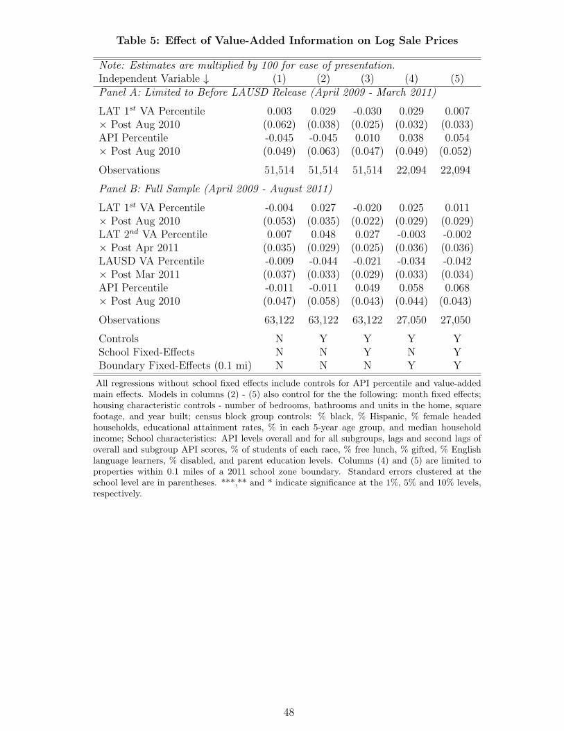
Table 5: Effect of Value-Added Information on Log Sale Prices

Note: Estimates are multiplied by 100 for ease of presentation.Independent Variable ↓ (1) (2) (3) (4) (5)Panel A: Limited to Before LAUSD Release (April 2009 - March 2011)

LAT 1st VA Percentile 0.003 0.029 -0.030 0.029 0.007× Post Aug 2010 (0.062) (0.038) (0.025) (0.032) (0.033)API Percentile -0.045 -0.045 0.010 0.038 0.054× Post Aug 2010 (0.049) (0.063) (0.047) (0.049) (0.052)

Observations 51,514 51,514 51,514 22,094 22,094

Panel B: Full Sample (April 2009 - August 2011)

LAT 1st VA Percentile -0.004 0.027 -0.020 0.025 0.011× Post Aug 2010 (0.053) (0.035) (0.022) (0.029) (0.029)LAT 2nd VA Percentile 0.007 0.048 0.027 -0.003 -0.002× Post Apr 2011 (0.035) (0.029) (0.025) (0.036) (0.036)LAUSD VA Percentile -0.009 -0.044 -0.021 -0.034 -0.042× Post Mar 2011 (0.037) (0.033) (0.029) (0.033) (0.034)API Percentile -0.011 -0.011 0.049 0.058 0.068× Post Aug 2010 (0.047) (0.058) (0.043) (0.044) (0.043)

Observations 63,122 63,122 63,122 27,050 27,050

Controls N Y Y Y YSchool Fixed-Effects N N Y N YBoundary Fixed-Effects (0.1 mi) N N N Y Y

All regressions without school fixed effects include controls for API percentile and value-addedmain effects. Models in columns (2) - (5) also control for the the following: month fixed effects;housing characteristic controls - number of bedrooms, bathrooms and units in the home, squarefootage, and year built; census block group controls: % black, % Hispanic, % female headedhouseholds, educational attainment rates, % in each 5-year age group, and median householdincome; School characteristics: API levels overall and for all subgroups, lags and second lags ofoverall and subgroup API scores, % of students of each race, % free lunch, % gifted, % Englishlanguage learners, % disabled, and parent education levels. Columns (4) and (5) are limited toproperties within 0.1 miles of a 2011 school zone boundary. Standard errors clustered at theschool level are in parentheses. ***,** and * indicate significance at the 1%, 5% and 10% levels,respectively.

48

Table

6:Effect

ofValue-A

ddedIn

form

ation

on

LogSale

Price

s-Altern

ativeM

odels

Note:Estim

atesforallmodelsexcept(3)are

multiplied

by100forease

ofpresentation.

IncludeStd

Include%

Teachers

Include%

Teachers

Use

Whether

Interact

with

Dev

ofCurrent

inVA

Quintile

inVA

Quintile

Schoolin

#of

Charters

Teacher

VA

(NoSchool

VA)

VA

Quintile

w/in1Mi

(1)

(2)

(3)

(4)

(5)

LAT

1stVA

Pctl

-0.029

-0.044

-0.052**

×Post

Aug201

0(0.025

)(0.031

)(0.025)

APIPctl

0.011

0.03

60.02

80.037

0.042

×PostAug20

10(0.048)

(0.045

)(0.043

)0.046

(0.045)

LAT

Teacher

VA

0.007

Standard

Deviation

(0.099)

Teacher/SchoolVA

Quintile:

2ndQuintile

1.0

0.1

2.4

(6.5)

(6.3)

(2.1)

3rdQuintile

-0.0

-2.5

2.2

(6.9)

(6.5)

(2.4)

4thQuintile

1.1

-2.2

-1.9

(7.4)

(6.9)

(2.3)

5thQuintile

1.3

-3.4

-0.9

(7.0)

(5.7)

(2.0)

LAT

1stVA

0.008

×Charters

w/in

1Mi

(0.010)

Observation

s50

,365

50,365

50,365

51,514

51,514

Thedatacover

April20

09throughMarch

2011

,prior

toLAUSD’s

releaseof

theirvalue-ad

ded

measure.Allregression

control

forthefollow

ing:

mon

thfixed

effects;school

zonefixed

effects;hou

singcharacteristiccontrols

-number

ofbed

room

s,bathroomsandunitsin

thehom

e,squarefootag

e,an

dyearbuilt;

censusblock

grou

pcontrols:%

black,%

Hispan

ic,%

female

headed

hou

seholds,ed

ucation

alattainmentrates,%

ineach

5-yearag

egroup,an

dmedianhou

sehold

income;

schoolcharacteristics:APIlevelsoverallan

dforallsubgrou

ps,lags

andsecondlagsofoverallan

dsubgrou

pAPI

scores,%

ofstudents

ofeach

race,%

free

lunch,%

gifted

,%

Englishlangu

agelearners,%

disab

led,an

dparented

ucation

levels.

Column(4)alsocontrolsforthenumber

ofcharterschoolswithin

1mileof

theproperty.Standarderrors

clustered

attheschool

level

are

inparentheses.**

*,**

and*indicatesign

ificance

atthe1%

,5%

and10%

levels

49

Table 7: Effect of Value-Added Information Relative to Exist-ing Information on Log Sale Prices

Note: Estimates for all models are multiplied by 100.

Primary All Primary & AllAPI Factor Factors Factors(1) (2) (3) (4)

LAT - API Percentile -0.022× Post Aug 2010 (0.024)LAT - 1st Factor Percentile -0.021 0.016× Post Aug 2010 (0.025) (0.050)LAT - Mean of Factor Percentiles -0.032 -0.051× Post Aug 2010 (0.026) (0.048)API Percentile -0.010 0.003 0.023× Post Aug 2010 (0.046) (0.046) (0.059)

Observations 51,514 51,458 51,514 51,458

The data cover April 2009 through March 2011, prior to LAUSD’s release of theirvalue-added measure. The estimates in column (1) show the difference between theLA Times first release VA percentile and the API percentile. The second column usesthe difference between the LA Times percentile and the percentile of the first primaryfactor component from the factor model discussed in the text. In column (3), we usea weighted average of the factor ranks, where the weights are the percentage of thevariance explained by each factor. In column (4), we use both the difference betweenthe LA Times VA percentile and the first factor and the difference between the LATimes VA percentile and a weighted average of all other factors. All regression controlfor the following: month fixed effects; school zone fixed effects; housing characteristiccontrols - number of bedrooms, bathrooms and units in the home, square footage,and year built; census block group controls: % black, % Hispanic, % female headedhouseholds, educational attainment rates, % in each 5-year age group, and medianhousehold income; school characteristics: API levels overall and for all subgroups,lags and second lags of overall and subgroup API scores, % of students of each race,% free lunch, % gifted, % English language learners, % disabled, and parent educationlevels. Standard errors clustered at the school level are in parentheses. ***,** and *indicate significance at the 1%, 5% and 10% levels, respectively.

50

Table

8:Effect

ofValue-A

ddedIn

form

ation

on

LogSale

Price

s-Specifica

tion

Check

s

Note:Estim

atesforallmodelsare

multiplied

by100forease

ofpresentation.

AddCen

sus

Exclude

Use

Lim

itLim

itDrop

Drop

Drop

Drop

3No

Include

Tract

Lagg

edSale

to0-2

to3+

Imputed

Properties

w/

Properties

w/

Multi

Mon

thAPI*

HighSale

FE

API

Levels

Bed

room

sBed

room

sSales

>8Bed

room

s>

500

0sf

Unit

Lead

Post

Prices

(1)

(2)

(3)

(4)

(5)

(6)

(7)

(8)

(9)

(10)

(11)

(12)

LAT

1stVA

Pctl

-0.041

*-0.028

-120

.2-0.010

0.00

5-0.049

**-0.027

-0.029

-0.017

-0.023

-0.029

0.078

×PostAug20

10(0.024)

(0.024

)(82.3)

(0.029

)(0.017

)(0.025

)(0.024

)(0.024

)(0.016)

(0.030)

(0.024)

(0.080)

APIPctl

0.004

0.013

319

.6*

0.00

6-0.018

0.04

6-0.002

0.006

-0.003

0.045

0.082

×PostAug20

10(0.040)

(0.036

)(193.1)

(0.049

)(0.029

)(0.044

)(0.044

)(0.044

)(0.033)

(0.039)

(0.141)

Observations

51,514

51,514

51,514

19,191

30,189

47,926

51,044

50,959

45,575

51,514

51,514

54,188

ThedatacoverApril200

9throughMarch

2011

,prior

toLAUSD’sreleaseof

theirvalue-ad

ded

measure.Allregressioncontrolforthefollow

ing:

mon

thfixed

effects;school

zonefixed

effects;hou

singcharacteristic

controls-number

ofbed

room

s,bathroom

san

dunitsin

thehom

e,square

footage,an

dyearbuilt;censusblock

grou

pcontrols:

%black,%

Hispan

ic,%

female

headed

households,ed

ucation

alattainmentrates,%

ineach

5-yearag

egrou

p,andmed

ianhouseholdincome;

school

characteristics:

API

levelsoverallan

dforallsubgrou

ps,

lagsan

dsecondlags

ofoverallan

dsubgrou

pAPIscores,%

ofstudents

ofeach

race,%

free

lunch,%

gifted

,%

Englishlangu

age

learners,%

disab

led,an

dparented

ucationlevels.

Standarderrors

clustered

attheschool

level

arein

parentheses.***

,**an

d*indicatesign

ificance

atthe1%

,5%

and

10%

levels,

respectively.

51

Table 9: Effect of Value-Added Information on Log SalePrices - Interactions Between VA Measures

Note: Estimates for all models are multiplied by 100 for ease of presentation.

(1) (2)

LAT 1st VA Percentile -0.021 -0.018× Post Aug 2010 (0.023) (0.022)

LAT 2nd VA Percentile 0.026 0.029× Post Apr 2011 (0.026) (0.027)

LAUSD VA Percentile -0.023 -0.017× Post Mar 2011 (0.033) (0.029)

LAT1 & LAUSD Same Quintile -0.852× Post Mar 2011 (3.968)

LAT1 VA Percentile 0.093× LAT1 & LAUSD Same Quintile (0.163)× Post Mar 2011

LAUSD VA Percentile -0.081× LAT1 & LAUSD Same Quintile (0.168)× Post Mar 2011

LAT1, LAT2 & LAUSD Same Quintile 1.938× Post Apr 2011 (5.601)

LAT1 VA Percentile -0.201LAT1, LAT2 & LAUSD Same Quintile (0.307)× Post Apr 2011

LAT2 VA Percentile 0.305LAT1, LAT2 & LAUSD Same Quintile (0.312)× Post Apr 2011

LAUSD VA Percentile -0.148LAT1, LAT2 & LAUSD Same Quintile (0.254)× Post Apr 2011

API Percentile 0.049 0.037× Post Aug 2010 (0.043) (0.042)

Observations 63,122 63,122

The data cover April 2009 through September 2011 and are at the propertysale level. The pooled LA Times value-added variable uses the value-added per-centile from the August 2010 release until May 2011 at which point the variableis replaced with the VA percentile from the May 2011 (2nd) release. All regres-sions include school and month fixed-effects along with controls for API, twoyears of lagged API, API percentile, and the school’s rank relative to comparisonschools defined by the California Department of Education. School character-istics include, % of students of each race, % free lunch, % gifted, % Englishlanguage learners, % disabled, and parent education levels. Neighborhood char-acteristic controls are at the census tract level and include % of the populationwho are adult, minor, senior, foreign born, of each race, speak a language otherthan English, and who lived in the same house one year prior, the % of adultswho are married, institutionalized, veterans, of each education level, in the la-bor force, and unemployed, % of households vacant and owner-occupied, averagehousehold size, family size, commute time and household income, the percentof households with children, single-parent families, receiving social security, re-ceiving cash public assistance, and receiving food stamps and the poverty rate.Housing characteristic controls include the number of bedrooms, bathrooms andunits in the home, square footage, and year built. Housing characteristics arealso interacted with a linear time trend. Standard errors clustered at the schoollevel are in parentheses.***,** and * indicate significance at the 1%, 5% and 10%levels, respectively.

52

Online Appendix: Not for Publication

53

Figure

A-1:Effect

ofValue-A

dded

Inform

ation

on

Log

SalesPrice

by

Month

ofSale,In

cluding

All

Value-A

dded

Releases

Initi

al R

elea

se in

Aug

201

0U

pdat

e R

elea

se in

May

201

1

−.006−.004−.0020.002.004Impact Estimate

−15

−10

−5

05

10M

onth

(0

is S

epte

mbe

r 20

10)

LAT

imes

1st

Val

ue−

Add

ed

Initi

al R

elea

se in

Aug

201

0U

pdat

e R

elea

se in

May

201

1

−.01−.0050.005Impact Estimate

−15

−10

−5

05

10M

onth

(0

is S

epte

mbe

r 20

10)

LAT

imes

2nd

Val

ue−

Add

ed

Rel

ease

in A

pr 2

011

−.0020.002.004.006.008Impact Estimate

−15

−10

−5

05

10M

onth

(0

is S

epte

mbe

r 20

10)

LAU

SD

Val

ue−

Add

ed

Rel

ease

in A

ug 2

010

−.004−.0020.002.004Impact Estimate

−15

−10

−5

05

10M

onth

(0

is S

epte

mbe

r 20

10)

AP

I

Theestimatesin

allpan

elscomefrom

asingle

regression

andshow

theim

pactof

anincrease

invalue-ad

ded

percentile

onlogsale

price

bymon

th,using

each

qualitymeasure.Controlsincludeschool

fixed

effects,mon

thof

saleindicators,within-districtAPIpercentile,overallAPIan

dbyracial/ethnicgrou

p,

twoyears

ofalllaggedAPImeasures;

Hou

singcharacteristic

controls-thenumber

ofbed

room

s,bathroom

sandunitsin

thehom

e,squarefootage,

and

yearbuilt;

school

characteristiccontrols-percentof

students

ofeach

race,percentfree

lunch,percentgifted

,percentEnglishlangu

agelearners,

percent

disab

led,an

dparented

ucation

levels;neigh

borhoodcharacteristic

controlsat

thecensusblock

grou

plevel

-percents

ofthepop

ulation

ineach

agegrou

p,

withless

than

ahighschooldiploma,withahighschool

diploma,

withsomecollege,

andwithaBA

ormore,whoare

black,whoareHispan

ic,an

dwho

arefemaleheaded

householdswithchildrenas

wellas

med

ianincome.

Thedottedlines

arethebou

ndsof

the95%

confiden

ceintervalsthat

arecalculated

usingstan

dard

errors

clustered

attheschool

level.

54

Table A-1: Relationship Between Having Sale Price Imputed and Observable Character-istics of Property

April 2009 to March 2011 April 2009 to September 2011

School Characteristics

API Growth Percentile 0.00000 0.00004(0.00021) (0.00018)

Share Black 0.00272** 0.00236**(0.00135) (0.00114)

Share Hispanic 0.00234** 0.00191**(0.00110) (0.00091)

Share API 0.00009 0.00043(0.00074) (0.00068)

Share FRP 0.00037 0.00066(0.00055) (0.00047)

Share Gifted 0.00092 0.00057(0.00073) (0.00061)

Share ELL -0.00183** -0.00153**(0.00078) (0.00064)

Share Speced -0.00106 -0.00054(0.00113) (0.00096)

Enrollment -0.00006 -0.00003(0.00007) (0.00005)

Share Parents HS Grad -0.00016 -0.00006(0.00105) (0.00079)

Share Parents Some Col -0.00014 -0.00018(0.00091) (0.00074)

Share Parents BA 0.00051 0.00007(0.00102) (0.00081)

Share Parents Grad Schl 0.00112 -0.00009(0.00137) (0.00109)

Property Characteristics

# Units 0.00458** 0.00676***(0.00227) (0.00205)

Year Built -0.00010*** -0.00009***(0.00001) (0.00001)

# Bedrooms 0.00361** 0.00291**(0.00149) (0.00137)

# Bathrooms 0.00321* 0.00361**(0.00177) (0.00160)

Square Footage/1000 -0.00490** -0.00664***(0.00225) (0.00220)

Census Block Characteristics

% Hispanic 0.01086 0.01680(0.02492) (0.02177)

% Black 0.01673 0.02355(0.02281) (0.02174)

% HS Grad -0.01860 -0.01880(0.02699) (0.02548)

% Some College -0.00903 -0.01202(0.02505) (0.02311)

% College Grad -0.01535 -0.00566(0.02945) (0.02706)

% Female Head -0.04305** -0.03503**(0.01820) (0.01690)

Median Income/1000 -0.00008 -0.00007(0.00007) (0.00006)

Observations 51,514 63,122

The data cover April 2009 through September 2011. All regression control for month fixed effects and school zone fixedeffects. Standard errors clustered at the school level are in parentheses. ***,** and * indicate significance at the 1%, 5%and 10% levels, respectively.

55

Table A-2: Effect of Value-Added InformationUsing Quintiles ofVA - All Releases

LAT 1st VA Percentile 2.79× Post Aug 2010 × Quartile 2 (1.92)

LAT 1st VA Percentile 1.59× Post Aug 2010 × Quartile 3 (2.1)

LAT 1st VA Percentile -2.61× Post Aug 2010 × Quartile 4 (2.61)

LAT 1st VA Percentile -2.13× Post Aug 2010 × Quartile 5 (2.53)

LAUSD VA Percentile -2.79× Post Apr 2010 × Quartile 2 (1.77)

LAUSD VA Percentile -2.19× Post Apr 2011 × Quartile 3 (1.86)

LAUSD VA Percentile -0.67× Post Apr 2011 × Quartile 4 (1.97)

LAUSD VA Percentile -3.03× Post Apr 2011 × Quartile 5 (2.72)

LAT 2nd VA Percentile -0.31× Post May 2011 × Quartile 2 (2.28)

LAT 2nd VA Percentile 3.71× Post May 2011 × Quartile 3 (2.26)

LAT 2nd VA Percentile 0.89× Post May 2011 × Quartile 4 (2.69)

LAT 2nd VA Percentile 3.91× Post May 2011 × Quartile 5 (3.36)

API Percentile 0.75*× Post Aug 2010 (0.04)

Observations 63,122

The data cover April 2009 through March2011, prior to LAUSD’s release of theirvalue-added measure. All regression con-trol for the following: month fixed effects;school zone fixed effects; housing char-acteristic controls - number of bedrooms,bathrooms and units in the home, squarefootage, and year built; census block groupcontrols: % black, % Hispanic, % femaleheaded households, educational attainmentrates, % in each 5-year age group, and me-dian household income; school character-istics: API levels overall and for all sub-groups, lags and second lags of overall andsubgroup API scores, % of students of eachrace, % free lunch, % gifted, % English lan-guage learners, % disabled, and parent ed-ucation levels. Standard errors clustered atthe school level are in parentheses. ***,**and * indicate significance at the 1%, 5%and 10% levels, respectively.

56

Table A-3: Effect of Value-Added Information Relative to Mean of Geographic andEthnic Markets

Note: Estimates for all models are multiplied by 100.

Geographic Markets Ethnic MarketsOther Schools Within X Miles of School “High”: ≥ 25%

2 mi 4 mi 6 mi 8 mi 10 mi of Race in School(1) (2) (3) (4) (5) (6)

LAT 1st VA Percentile -0.039* -0.043* -0.039* -0.042* -0.043* -0.046*× Post Aug 2010 (0.023) (0.024) (0.024) (0.024) (0.025) (0.025)Mean VA Nearby Schools 0.027 0.022 -0.174 0.041 0.195× Post Aug 2010 (0.048) (0.077) (0.106) (0.123) (0.152)High Black × Mean VA Other High Black -0.026× Post Aug 2010 (0.064)High Hisp × Mean VA Other High Hisp 0.080× Post Aug 2010 (0.076)High White × Mean VA Other High White 0.028× Post Aug 2010 (0.038)High Asian × Mean VA Other High Asian 0.083× Post Aug 2010 (0.055)API Percentile 0.032 0.036 0.061 0.035 0.027 0.030× Post Aug 2010 (0.044) (0.044) (0.044) (0.044) (0.045) (0.049)

Observations 49,809 50,873 50,873 50,873 50,873 51,514

The data cover April 2009 through March 2011, prior to LAUSD’s release of their value-added measure. All regressioncontrol for the following: month fixed effects; school zone fixed effects; housing characteristic controls - number ofbedrooms, bathrooms and units in the home, square footage, and year built; census block group controls: % black,% Hispanic, % female headed households, educational attainment rates, % in each 5-year age group, and medianhousehold income; school characteristics: API levels overall and for all subgroups, lags and second lags of overall andsubgroup API scores, % of students of each race, % free lunch, % gifted, % English language learners, % disabled,and parent education levels. Standard errors clustered at the school level are in parentheses. ***,** and * indicatesignificance at the 1%, 5% and 10% levels, respectively.

57

Table

A-4:Effect

ofValue-A

ddedIn

form

ationonLogSale

Price

s-Specifica

tionCheck

s,AllReleases

Note:Estim

atesforallmodelsare

multiplied

by100forease

ofpresentation.

AddCensus

Exclude

Use

Lim

itLim

itDrop

Drop

Drop

Drop

3No

Include

Summer

Tract

Lagged

Sale

to0-2

to3+

Imputed

Properties

w/

Properties

w/

Multi

Mon

thAPI*

HighSale

Only

FE

API

Levels

Bedroom

sBedroom

sVA

>8Bedroom

s>

5000sf

Unit

Lead

Post

Prices

(1)

(2)

(3)

(4)

(5)

(6)

(7)

(8)

(9)

(10)

(11)

(12)

(13)

LAT

1stVA

Pctl

-0.026

-0.028

-110.3

-0.006

0.008

-0.030

-0.017

-0.018

-0.009

-0.011

-0.011

-0.062

-0.014

×PostAug2010

(0.021)

(0.022)

(73.3)

(0.026)

(0.017)

(0.023)

(0.022)

(0.021)

(0.016)

(0.022)

(0.022)

(0.146)

(0.058)

LAT

2ndVA

Pctl

0.021

0.024

55.0

0.046

0.006

0.031

0.023

0.026

0.031

0.003

0.025

0.080

0.028

×PostApr2011

(0.022)

(0.025)

(90.8)

(0.032)

(0.021)

(0.024)

(0.025)

(0.025)

(0.020)

(0.036)

(0.025)

(0.122)

(0.060)

LAUSD

VA

Pctl

-0.007

-0.014

-100.2

-0.029

0.024

-0.027

-0.019

-0.019

-0.022

-0.034

-0.019

-0.150

-0.042

×PostMar2011

(0.027)

(0.027)

(97.2)

(0.029)

(0.022)

(0.027)

(0.029)

(0.028)

(0.019)

(0.038)

(0.028)

(0.098)

(0.044)

APIPctl

0.023

0.048

457.8**

0.021

0.002

0.069*

0.035

0.035

0.011

0.081***

0.258*

0.173**

×PostAug2010

(0.032)

(0.031)

(197.0)

(0.044)

(0.025)

(0.041)

(0.041)

(0.041)

(0.032)

(0.029)

(0.152)

(0.074)

Observation

s63,122

63,122

63,122

23,444

37,061

58,546

62,504

62,401

55,708

63,122

63,122

66,174

20,307

ThedatacoverApril2009

through

September

2011.Allregression

control

forthefollow

ing:

month

fixed

effects;school

zonefixed

effects;hou

singcharacteristiccontrols-number

of

bedroom

s,bathroomsan

dunitsin

thehom

e,squarefootage,andyearbuilt;censusblock

groupcontrols:

%black,%

Hispan

ic,%

femaleheaded

hou

seholds,education

alattainment

rates,

%in

each

5-yearage

group,an

dmedianhouseholdincome;

school

characteristics:APIlevelsoverallan

dforallsubgroups,

lags

andsecondlags

ofoverallandsubgroupAPI

scores,%

ofstudents

ofeach

race,%

free

lunch,%

gifted,%

Englishlanguage

learners,

%disab

led,an

dparenteducation

levels.

Standarderrors

clustered

attheschool

level

arein

parentheses.***,**an

d*indicatesign

ificance

atthe1%

,5%

and10%

levels,

respectively.

58