DOCUMENT RESUME

ED 222 554 TM 820 708

AUTHOR Mislevy, Robert j.; And OthersTITLE Scale-S'core Reporting of National Assessment Data

(Final Report).INSTITUTION Education Commission of,the States, Denver, Colo.

National Assessment of Educational.Progress.SPONS AGENCY National Inst. of Education (ED), Washington, DC.

'PUB DATE Feb 82GRANT NIE-G-80-0003NOTE. 130p.; For related documents, see TM 820 707-712 and

TM 820 716.-0

EDRS PRICE MF01/PC06 Plus iicistage.DESCRIPTORS Educational Assessment; Item Analysis; *Item

Sampling; *Latent Trait Theory; *MathematicsAchievement; National Surveys; Racial Differences;*Scaling; *Scores; Secondary Education; SexDifferences; Test Constrzction; Test'Reliability

.IDENTIFIERS National Assessment of Educational Progress; *NIE ECSNAEP Item Development Project; UnidimensionalScaling; Unit of Analysis Problems

ABSTRACTAn approach was developed'based on item-response

models defined at the level of salient subject groups rather than atthe level of individuals, designed for use with mul,tiple-matrix

.sampling designs. In each of three National Assessment of. EducationalProgress (NAEP) mathematics subtopics, Reiser's group-effects latenttrait model was fitted to the proportions of correct response toitems as observed in the cells of a design. Item parameters andcontrasts among demographic groups were estimated in each of fourdata sets: 1972-73 and 1977-78 data for 13-year-olds and17-year-olds. Based on itemi-common to two or more data sets, resultswere linked across ages and over time in each subtopic. Itemparameters and group averages were obtained on scales common acrossages-and years. Successful calibration and linking in all subtopicsdemonstrates the feasibility of applying item-response methods tosparse sampling designs. However, scaling must be accomplished withinfairly narrowly-defined skill areas, such as the NAEP subtopics, if

the integrity of scales is to be maintained. Item response scaling ofNAEP test booklets as a whole is discouraged. Primary type ofinformation provided by the report: Results (Secondary Analysis).(Author/CM)

***********************************************************************Reproductions supplied by EDRS are the best that can be made

from the original document.******************,*********************************** *****************

41

SCALE SCORE PEPOPTING nF

NATIONAL ASSESSMENT PATA

a

U.S. DEPARTMENT OF EDUCATIONNATIONAL INSTITUTE OF EDUCATION

EDUCATIONAL RESOURCES INFORMATIONCENTER (ERIC)

S. This document has been reproduced asmceived from the person or organizationoriginaung itMinor changes have been made to improvereproduction quality.

Points Of view or opinions stated in this do:m-ment do not necessarily represent official N1Eposition or policy

SCALE-SCORE REPORTING OF NATIONAL ASSESSMENT DATA

(Final report)

Robert 3: Mislevy

International Educational Services

Mark R. Reiser

Indiana University

Michele Zimowski

University of Chicago

February, 1982

The work upon which this publication is based is performed pur-suant to Grant NIE-G-80-0003 of the National Institute of Educa-tion.. It does not, however, necessarily reflect the views of thatagency.

SCALE-SCORE REPORTING OF NATIONAL ASSESSMENT DATA

Robert J. Mislevy, International Educational Services

Mark R. Reiser, Indiana University

Michele Zimcwski, University of Chicago

Abstract.

Perhaps the two most significant advances in educational mea-.surement over the past twenty years have been item response theoryand multiple-matrix sampling designs. Unfortunately, few.re-searchers interest4d in assessment have been able to. enjoy thefull benefits of both advances simultaneously; the current methodsof item response theory,cannot deal with the sparse data (at thelevel'of.individuals) that characterize the most efficient samp-ling designs. This research develops an Approach based on item-response models defined at the level of salient subject groupsrather than at the level of individuals, designed for use with themost efficient multiple-matrix designs, i.e., those in which eachsampled subject is presented at most one item per scale.

In each of tlii-ee NAEP mathematics subtopics, Reiser's group-effects latent trait model Was fit to the proportions of correctresponse to items as observed in the cells Of a des,ign includingsex, race/ethnicity, region of the country, and size and type ofcommunity. ,

Item-parameters and contrasts among demographic groupswere thus estiwated in each of four age/year data sets: 1972/73and 1977/78 data for 13-year olds and 17-year olds. (Data weretaken from NAEF' public release tapes from these age/years and fromthe NAEP mathematics 1972/78 "change" tape.) Based on\items commonto two or more age levels and/or assessment years, results werelinked across ages and over time in each subtopic. Item para-meters and group averages were then obtained on scales commonacross ages and years, despite the fact that different (but over-lapping) sets of items had been administered in each age/year.

Successful calibration and linking in all three subtopics demon-strates the feasibility of applying item-response methods to thesparse sampling designs of moern assessment. It is seen, how-ever, that scaling must be accomplished within fairly narrowly-defined skill areas, such as the NAEP subtopics, if the integrityof scales across demographic groups and over time is to be main-tained. In particular, item response scaling of NAEP test book-lets as a whole is to be most strongly discouraged as it yirtuallyguarantees item parameter drift over time and poor fit to uni-dimensional item response models.

`za

PREFACE

fCONTENTS

I. INTRODUCTION AND BACKGROUND Page 1

The nature of educational assesspentMultiple-matrix sampling designgMethods of reporting assessinent resultsProblem statement

II. ITEM RESPONSE-CURVa METHODS FOR ASSESSMENT Page 13

Introduction to item response-curve theory -

Application to multiple-matrix samples of responsesReiser's model for group effectsLinking results across assessments

III. EXAMPLES FROM NAEP'S ASSESSMENTS OF MATHEMATICS . Page 38

Introduction to the examplesMethodology -

Results

IV. CONCLUSIONS _Page 52

BIBLIOGRAPHY

APPENDICES

A. 'Technical presentation of Reiser's model for group effectsB. A minimum Chi-square solution for linking calibrations

from forms with an arbitrary desi6n of overlapC. A computer program program for linking calibrationsD. Comments op the NAEP public-use data tapes

PREFACE

Item response-curve models have triggered no less than arevolution in educational measurement. Little wonder, since somany measurement problems that are difficult or impossible tosolve within the framework of classical psychometric theory becomequite tractable under the item response-curve approach; examplesinclude analyses of the information that items'and tests provideat various levelg of ability, measurement on an invariant scalefrom any subset of of calibrRted items, and simplified test.-

equating procedures.

To date these benefits have not been realized in the NationalAssessment of Educational Progress. the primary reason, perhaps,is NAEP's use of multiple-matrix sampling designs--efficientprocedures, guaranteed to provide, economical estimates of grouplevel attainment% Sufficieritly precise estimates of group-levelattainment may be obtained by administering only a few items frota given skill=area to any selected subject. Unfortunatedy, thecurrent state of item response-curve tlieory cannot handle datasuch as gathered by NAEP, wherein each subject,responds to too fewitems in a specific skill area to permit the stable estimation ofhis ability level.

- - This project is intended to further the extension of itemresponse-curve theory to the assessment setting. The foundatiqnsof the present work appeared in the estimation procedures outlinedin Bock (1976) that were later put into practice with the Cali-fornia Assessment PrograW(Bock, 1979; Bock and Mislevy, 1981);item response curve models are in these applications-defined notat the level of individuals but at, the level of salient groups ofindividuals. Reiser's (1980) dissertation research introduced agroup-level item response-curve-model that is particularly suitedto NAEP data, addressing characteristics of test items and per-formances in the cells of a design on persons. The present workdevelops procedures to link such results across assessment yearsand/oe age groups. Examples are drawn from the 1972/73 and1977/78 NAEP mathematics assessments.

1

' CHAPTER I

INTRODUCTION AND BACKGROUND

The Nature of Educational Assessment

The purpose of educational'assessment is to provide infor-

t

mation about the levels of skifls or attitudes in specified popu-

lations of; subjects. .Results may bbvcompared from one population

to another or from one pointjn tim to another, in order to*study

the effects of educational treatments or societal trends. The

distinguishing feature of assessments, however, ies their focus on

groups rather than.on individuals.

By virtue of its distinct purposes, assessment requires a

different technology than its ctose cousin, educational meas-

. urement. The "true-score" models of traditional psychometrics1.

concern the meastiement of individual sUbjectS rather than groups

of subjects; it is not surprising that the strategies of

test construction designed to proyide optimal measurement of

individuals are not optimal for assessment. WhiJe borrowing

heavily from the models and the concepts of educational mea-

surement, assessment technology has gainfully employed ideas'from

othe'r fields ds well, notably those of opinion survey sampling and

sampling design 'theory.

-1-

The state Of the art of,assessment in the United States is

exemplified by the National Assessment of EducatiorL Progress

(NAEP) and the Californi.a Assessment Program (CAP). These two

programs have, since.their inceptions over a decade ago, been0

proving grounds for measurement and statistical advances designed

to obtain efficient and economical estimates of group-level at-

tainment. Our-attention will focus primarily on the National

.Assessment, although discussion of certain topics will be clari-

fied with examples from the California Assessment.

Tne National Assessment of Educational Progress charts levels

of attainment in ten broad areas, including Reauing, Science,

Mathematics, and Writing Skills. Each area is assessed periodic-..

ally, usually once every four or five years. Information is

gathered mainly through the administration of multiple-choice and

open-ended-tasks from the target area to subjects selected in the.

NAEP sampling design. Demographic and_educat_ional background data

are also obtained for each sampled subject.__Results are reported

as proportions of correct response to individual items and clus-

ters of iteMs, for groups of individuals defined by demographic

Niariables such as, age, sex, region of the country, size of com-

munity, and so on.

Comparing NAEP results over time or across age-groups re-

quires measurement on an invariant scale. Proportions of correct

response for a given itet may be compared across all the assess-

ments in which it wasoadministered... but dertainly trends in,

-2-

1

say, Mathematics skill are inadequately revealed by performance on

any single item. To overcome the idiosyncracies0of individual

items, information must be combined over several items testing the

same essential skills.

Average percents-correct crier clusters of items,may instead

be followed, but only as long as the composition of the cluster

does not change. NAEP uses-this option at present, but it is

hampered by the fact that typically'one fourth.of the items in each

assessment are released to the public and retired from the item

pool. Comparisons across assessments of average percents-correct

t,of clusters of items will become less reliable as the numbers of

common items shrink over the years.

This report explores methodsby which mOdern item response-

curve,measurement theory may be applied to the assessment setting

tb solve the problems of cHarting progress over time. The next

section of this chapter reviews the basics of multiplel-matrix0

sampling theOry, the development which has contributed so much to

the success Of large-scale assessments such as NAEP to date. It

is upon this sampling frameworl that measurement models-must build

if they are truly to advance the practice of assessment. Next,,

the current practices of reporting assessment results are

reviewed. Their limitations and prospects for overcoming them are

discussed. Vie chapter concludes with a succinct statemen of the

'fi'l°'-'

objectives of the present research.

-3-

Multiple-Nratrix Samplj.ng,'

The accountability movement of the 1960's inspired the'cre-

ation of a number'of local and statewide testi'hg prOvams intended

.to provide fee4back about the,effects of public expenditures on

education. The methodology employea in these programs was that of

standardized achievement testing. -Every pupil in a school or

classroom was admipistered an achievement test cOnsisting of as

many as -tWo hundred test items, an undertaking demandifig hours,or

even'days of classroom time from.each pupil. Designed to provide

maximal differentiation among students, these tests yield highly

accurate scores for each pupil in but a few broad skill areas.

Averages of pupil-level sopres obtained in such A scheme did

in4eed reflect levels'of performance in the school or classroom,

but in a most highly inefficient manner. The administration of

intensive every-pupil testing with traditional achievement tests

suffers several serious.deficiencies if it is only the group-level

results that are.necessary for discussion by the public and the

educational community; .Thelarge numbers of items which must be

administered to a student in a skdll area if distinttions are to

be made among, students are simply not necessary if only infor-

. mation about average levels of attainment in the group at.; a whole

is desired. Such a scheme expends scarce.educational resources to

measure each student much more- preciseli than is required in an

assesLment, but by providing results in only a few broadly-

conceived skill areas, offers little in the way of specific guid-

ancei for,impfoving the curriculum.

-4-

During same period, sample survey techniques were be-

coming a familiar and widely-accdpted mechanism for guaging the4

strength of various attjtudes and opinions among the pubiic,

mainly on issUes of social or politicgl relevance. Not'eVery

person is interviewed; not every person interviewed is asked all

the 'same questionS. Yet satisfattorily precise and reliable

information is' obtained.about the.prevalence of attitudes in the

public at large. Why not apply these same methods to,..educational

assessment?

0

At the request of William Turnbull, president of Educational

Testing Services, Frederic Lord Investigated the possibility of

estimating levels of ability in d population by means of "mul-,

tiple-matrlx sampling"--that is, by adMinistering diffe'rent sub-

sets of an item domain to different samples of persons,(Lord,

1962; Lor and Novick, 1968, Chaibter 11).

The simplest application of pulti e-matrlx sampling is in.

estimating the average item 'score in a populeion of N subjects

for an item pool. Of K test items. The average score that would be

obtained by administering every item to every subject can be

, approximated by observing the responses of, say, t different

random samples of n subjects each to random samples of k itemsdo

each,, (,This is referred to in the multiple-matrix sampling -liter-

ature as a t/k/n design.) ,The expected value of the average item

score over all such samples is the population average item score.

a

One 'of the,Most imporfant results ofLord's investigations

was the conclusion that the estimation of the population average

is most-precise for a given number of responges-when k=1; that is,

when the,responses for.different items have been obtained from,

non-overlapping samples of subjects. Stated simply, two responses

7 contain°more information abOut the pdpulation if they are from

different persons'than if they are from the same Person.

Pandey and Carlson (1976), in a study of data from the Cali-

fornia reading assessment, ford the effect to be generalizable.d

The eigror variance associated\with estimates of the population

mean was reduced almost four-fold 'when, for the same number of

responses,,forms of ten items each weredadminigtered to samples of

ten subjects each, as compared to a design undero,which the items

were administered as two fifty-ifem forms to ten subjects each.

Practical work generally requires a more complicated sampling

design than those describeeabove. In the California Assessment,

as an example, results must be reported individually for each

'school. In the National- Assessment, results must be reported for

the cells and the margins of A design based on demOgraphic vari-

ables.b Sampl'ing of subjects .must therefore be carried out within

levels of st'ratification in both cases, aklowing for: the possi-.

'bility of different selection'prObabilities within different cells

, to meet.requirements for-th'e precision of estimatio

a

Item pools are generally statified as well, into divisions of

increasingly narrower skill requirements. Ithegoa1 is to define

classes of items which are similarly affected by specific attrib-

utes of educational treatments, in order that treatments can be

monitored and modified as a result of the feedback from the asse-

ssment. Our attention in this paper will focus on items within

bhe finest level of stratification of the item pool, which, fol-

lowing the practice of the California Assessment,\we refer to as a

"skill element."

Reporting Assessment-Results

As noted above, comparisons of assessment results over time

and across assessments requires measurement on an invariant scale..

The method by.which this requirement is achieved in public opinion

survey research is to present subjects with questionS that remain

constant over time; by asking, for example', "Which,of these can-.

didetes would you vote for if the election were today?" of sub-

jects interyiewed during the six mcmths before th'e election, one.

may chart the flowoof public support behind the candidates.

Tyler's (1968) remarks and Womer's (1973) monograph suggest.that

this same method was originally intended for reporting the results

of the Nationaf Assessment of Educational Progress.

'The "fixed-item" approach to reporting the results of assess-

ments, as it,might be called, focuses on comparisons of perform-

ance between group's or across time on a single, specific task.

-7-

Jai

Interpretation is straight-forward as it applies to performance on

that particular item, but the problem lies in generalizing the

results. .The 1972/73 NAEP Mathematics,Assessment, for example,

presented 200 items to 13-year-olds alone; results for the cells

of a sex by race by size-and-type of community design would have

to be expressed as some ten thousand separate percent-correct

values. Comparisons across groups would vary across items as a

result of measurement error as well as with the skills tapped by

the items. How could such a preponderance of detail be suited to

general public dissemination or discussion?

Educational test items, unlike public opinion surveir ques-

tions, are not usually important in and of themselves, but instead

as representatives of a class of tasks requiring similar skills.

It is these generalized skills rather than the specific items that

are addressed by instruction, and it is this level at which as-

sessment results must be reported. The technology of educational

measurement, as it had developed by the early 1970's (see, for

example, Cronbach et al, 1972), was able to provide a framework

for generalizing results across test items within a skill area:

the "random-item" model.

Under the "random-item" approach to reporting the results of

assessments, the specific items4from a given skill area are con-

sidered a random sample from a population of items that, taken

together, defines the area. The average item score by group of

subjects to a randomly-selecte'd subset of these items is an esti-

-8-

1

mate of the group's average for the entire population of items in

the area. 9ecause results are averaged over a number of items,

peculiarities of item formats and distractors tend to cancel out,

revealing trends which underly performance on all the items in the If

skill area. Under this model, average item scores may be compared

across groups and over time even though different sets of items

may have been administered, as long as the set of items admin-

istered in each assessment has been chosen at random from an

invariant fpopulation of items.

The assumptions of the "random-item" approach are not,

unfortunately, met in general practice. The problem lies with the

requirement of randomly sampling items from an invariant item pool.

If comparisons are desired across age groups, for example, sub-

jects must be presented items from the same item pool; the effi-

ciency of estimation suffers if younger subjects are presented

just as many hard items as are necessary to tap the skills of

older subjects, and older subjects are presented too many'easy

items just so the younger subjects can be tested.

A more serious problem is the charting of results over time.

If item pools remain invariant, they cannot reflect new emphases

in educational treatments nor can they retire items which have

outlived their usefulness; neither can items be released to the

public to aid the interpretation of results without compromising

the integrity of the measurements. Yet if apparentlY desirable

revisions to certain items are carried out, the average item

-9-

scores estimated in 'different assessments are not comparable; they,

are estimates of performance in a shiftin collection of items,

perhaps harder or easier on the whole from one year to the next.

Changes in subjects' skill levels are confounded with changes in

the composition of the item pool.

The National Assessment, recognizing this problem, has re-

sponded"by reporting results that are to be compared over time in

two different ways.

For non=technical reports slated for public release, propor-

tions of items correct are reported over all items in a skill

area, despite modifications in the item pool and decidely non-

random selections of items in an assessment. The comparisons

implied by the figures for different years, although they do not

meet the assumptions required to assure meaningfulness, are con-

sidered useful nonetheless. And indeed they may be good approx-

imations of the comparisons that would have resulted under ideal

conditions; i.e., true random sampling in both years from,a fixed

pool of items.

For scientific investigations, NAEP provides reports and data

tapes based on only those items which appear on all the assess-

ments to be compared. The assumptions of the "randcm-item" model

may be met in this way, defining the skill area to be that which

is measured by the average of that specific collection of items.

Comparisons, restricted to these so-called "change items," suffer

-10-

1

from the culling of items that cannot be matched, in that poten

tially useful information from these items must be ignored. The

resources expended in gathering this information have not been

justified in this respect. Analyses of trends over time are

as well, as the set of items common to all assessments in ques-

tion tends to shrink when more time points are considered.

Similar problems in the measurement of individual subjects(

have been overcome with the advent of item response-curve (IRC)

'measurement models. An IRC model individually parameterizes each

t.est item in a suitable domain in terms of its relationship to an

underlying scale of ability. Subjects may then be measured on an

invariant scale of attainment, based on their responses to any

subset--not just a randomly selected subset--of items. The chal-

lenge is to apply the methods of IRC theory to the setting df

assessment, borrowing concepts and machinery to free reporting

from the constraints of classical test theory, while at the same

time building upon the multiple-matrix sampling framework.

Problem Statement

The object'ive of this research is to further the development ,

of one approach to applying item response-curve methods to

assessement data; namely, Reiser's (1980) 'group effects model,

which (1) allows the estimation of group-level parameters from

item responses obtained in an efficient multiple-matrix sampling

design, (2) yields these parameter estimates on a scale that is

invariant over time.and across groups, and (3) permits.the evolu-

tion of the item pool over time without degrading the integrity,or

the generality of the results. The steps we take to this end are

as follows:

1. Develop an algorithm for linking estimates from the Reiser

model across assessments. The approach will be based on a

proposal by Tucker (1948). Linear transformations are

determined to provide optimal agreement among estimates

from an arbitrary number of assessments, linked by an

arbitrary pattern of common items.

2. Demonstrate the use of the grclup-effects model and the

linking program with data from the NAEP 1972/73 and 1977/78

Mathematics AsseSsments. Scales will be linked agross

assessment years and across the 13- and 17-year-old age

groups in three skill areas:

-12-

1

(±

CHAPTER II

ITEM RESPONSE-CURVE METHODS FOR ASSESSMENT DATA

This chapter develops anapproach for adapting item4

response-curve methods t8 the assessment setting. The first

sectionris a brief review of item response-curve theory as it has

been developed for measuring individual subjects. Features and

properties of IRC models that will be important in our generaliza-

tion to group-level data'will be emphacized. The second section

discusses the notion of applying IRC methods to.data obtained from

multiple-matrix sampling designs. In particular we consider the

option of defining IRC models at the level of subject groups

rather than individuals. The third section is a non-technical

description of Reiser's group-effects, an IRC model defined at the

level of groups that is particularly well-suited to the'demo-

graphic stratifications used by the National Assessment. The

_

final section discusses the linking of results from the Reiser

model from one assessment to others, thus providing the continuity

of measurement necessary,for longitudinal analyses. (The topics

treated in the last tWo sections, the Reiser model and the linking

procedures, are treated in a more technical manner in Appendices A

and B respectively.)

-13-

Fundamentals of Item Response-Curve Theory

The models of item response-curve theory differ most radd-

cally from the models of traditional "true-score" psychometrics by

parameterizing test items individually in terms of their rela-

tionships to the underlying ability, rather than treaiing them as

random samples from a pool of interchangable items. Once a set of

items has been "calibrated" (i.e., the parameters of the items

have been estimated), a subject's ability can be estimated from

his responses to any subset of the items. This is the case even

when the items he has been presented are only easy ones or only

hard ones--assuming that the IRC moder fits the circumstances

reasonably well.

The heart of an IRC model is a mathematical equation for

the probability of a correct response to a particular, item by a

particular subject, in terms of one or more parameters that in-

dicate the subject's abiliy and one or more parameters describing

how responses to the item are influenced by ability.

To illustrate, we will consider the Birnbaum.2-parameter

logistic*item response-curVe model, which will be seen to share

many similarities with Reiser's group-effects model for assessment

data. The probability that Subject i will respond correctly"to

Item j is given by the following function:

exp[1.7 Aj (ei Bj)]Prob(Xij=1) (1)

1 + exp[1.7 Aj (ei Bj)]

where

-14-

Xij, the response, is 1 if it is correct and 0 if not,

exp is the exponentjal function,

Ai is the "ability" parameter of Subject i,

Aj is the "slope" parameter of Item j, and

Bj is the "threshold" parameter of Item j.

(The scaling constant 1.7 is included in this expression in'order

to make the item parameters in the Birnbaum logistic model match

more closely the item parameters in the normal ogive model.)

,The-function shown above describes how likely it is that a1

subject with a given ability will respond correctly to Item j.

This function.can be graphed, as in Figure 1: the item response

curve for Item j. It may be seen that subjects with very low

values of e have little chance of responding correctly., As A

increases, so do chances of responding correctly. For a subject

with an ability that has the value Bj (the threshold of Item j),

the chances of a,currect response are 50-50. As ability continues

to increase, chances of restionding correctly increase also until ,

it is nearly a certaknly at very high levels of ability.

When this model is fitted to data, it is capable of

accounting for the facts that--

(1) ome subjects perform better than others on the items

_in e.skill area.

(2) Some it ms in the area are easier than others..

(3) Some items ar more reliable indicators of the ability

-15-

than'othdrs.

Figure 2 shows three different item response curves on the same

:plot. It may be seen that, on the average, Item 3 is harder than

Item 2, which is harder than Item 1. It may also be seen that the

higher the value of,'an item's slope, the more sensitively an item

reacts to changes in subject ability. Item 2 is more informative

than Item ', which in turn is more informative than Item 3.

The manner in which subject and item parameters combine to

produce probabilities of correct response is illustrated in Tables

1 and 2. Table 1 shows, for the four hypothetical items and six

hypothetical subjects, the quantity 1.7 Aj (ei Bj). The orderly

relationships among the parameter values are most clear in this

chart, showing what are called the "logits" of correct response.

Table 2 transforms these logits to the more familiar units of

probabilities via Equation 1.

It may be noted at this point that the units for the subject

and item parameters are unique only up to a linear transformation.

That is, equivalent relationships may be expressed by transforming

all the parameters by the linear function f(x)=mx+b as follows:

ei* = m ei + b

Aj* = Aj / m

Bj* = m Bj b.

It may be readily verified that these transformed subject and item

parameters yield exactly the same probabilities of correct re-

sponse as the originals, since

-16--

PROB = 1.0

PRO13 = 0.5

PROB = 0.0 .

THETA -4 -3 -2 -1 0 1 2 3 4

PROB = 1.0

PROB = 0.5

?ROB = 0.0

THRESHOLD = -1.00

--SLOPEr-- 4400

FIGURE 1AN ITal CHARACTERISTIC CURVE

.

......

.;...-..

L. -3 7.2 -1 0 f 2 3 4

ITE:4 THRESHOLD. SLOPE--- -1 -2.00 .77

---. 2 -1.00 1.00.... 3 1.00 .50

FIG U E 2

SEVERAL ITi CdikRACTEH2TIC CURVES

TABLE 1LOGITS OF EXPECTED PROPORTIONS CORRECT

SUBJECT AiBj: -2.000

1.7 Aj: 1;000

ITEMS

-1.0000.500

1 -0.500 1.506 0.250

2 -1.500 0.500 -0.250

'3 0.500 2.500 0.750

4 -0.500 .1.500 0.250

5 1.000 3.000 1.600

6 0.000 2.000 0.500

1...060 2.0000.500 1.000

-0.750 -2.500

-1.250 -3.500

-0.250 -1.500

-0.750 -2.500

0.000 -1.000

0.500 -2.000

TABLE'2-EXPECTED PROPORTIONS CORRECT

SUBJECT

1

2

3

4

5

6

Ai

-0:500

-1.500

0.500

-0.500

1.000

0.000

1.7Bj:Aj:-,

-2.0001.000

.818

.622

p924

.818

.953

.881

ITEMS

-1.0000.500

.562

.438

.679

.56.:

.731

.622

1.000 2.0000.500 1.000

.321 .976

.223 .029

.438 .182

A21 .076

.500 .269

.378 .119

0

1.7 Aj* (Ai* - Bj*) = 1.7 Aj (Ai Bj).

The implication is-that when parameters are estimated for the Same

set of items from different sets of data, they can be expected to

differ by such as linear transformation. It is a practical prob-

.

lem to estimate the optimal transformation; various solutions and

proposals have been made by Tucker (1948), Lord and Novick (19-68),

and Haebera (1981).

Benefits of Item Response Curve Models

--Whena--76onest-i-on--of---subjects_l____r_e_sponses- -'o test items can_be

adequately summarized in terms of an item res onse-curve model

like the one described above, several benefits accrue:

Invariance with respect: to item selection. Once a collection

of items has been calibrated (i.e.,'the pai-amete'rs of the items

have been estim"ated), a subject's ability may be estimated on the

basis of his responses to any-subset of tlie items--randomly se-

lected or not. This means that, as dn example, younger students

may be'administered mostly easy ite,Fis while older students are

administered mostly difficult items from the same scale.

New items can be added to the domain. New items measuring'

the same trait'can be linked into an existing scale by administer-

itig them along with items thatllave already been calibrated. The

new items.can be calibrated from this data, then their fit to the

model verified before they are used to estimate subjects'

abilities.

-17-

U.

1

Z4

Flawed items can be corrected. ,Items found to-have flaws in

their grammar, format, or conception can be revised, then re-cal-

ibrated,into the domain as if they were new items.

Items can be dropped from the bank. Without affecting the

the scale of measurement,, items may be retired from use,*either

because they are outdated or because they will be used to illus-

trate the content area in 'reports releaied to the public.

r.Content-referencing of scotes. .The.scaled scores (e) from

IRC theory-are-defined-implioltly-by-the-probabilities..af_correot.

responses they imply for.each of the itemt ip the skill area. The

meaning of an ability -estimate,canbe interpreted, therefore, b30

inspecting.the content of the items with thresholds in that region'

.of the scale--without reference to the distribution of ability in

any population of subjects. Scale scotes may still be interpreted

in the more' familiar,manner of norm-referencing of course, with

the cpmpuation of percentiles, stanines, standard scores, Wand so

on, with iegard.to specified populations, of subjects.,

A

Linearity with external variables. Because IRC abilitf

estimates are'not subject to the flOor and ceiling,effects of.. .

, .

numbers-5right and percents-correct, they tend to have more l'inear,,

relai4 ships with external variables such as, SES, age, and years

of educatiOn.

Well-defined 'standard errors. Because items are large-sample

calibrated, they are considered 'fixed' rather that; 'random' from

-18-

a

a statistical pOint of vivw. For this reason, standard errors of

-estimating subjects' abilities, and, indirectly, reliabilities,

are easy to compute (seeeLord & Novick, 1968; Mislevy, 1981).

Moreover, these standard errdrs are correctly,expresse.d as a

function'of the ability itself rather than gratuitously and erron-.

eously assumed constant' as in classical,theory for'number-right

scores.*

Suitability for longitudinal studies. With the.use of alter-

' nate test forms Consisting oflitems from the same scale, IRC

I7

ability.estimates are amenable to the study of trends or program

effects.

I.

1,

Assumptions'of Item Response Curve Models

.

If an IRC,model is to fit data, the asumptions .of the model

must be reasonably well satisfied. The main asstimptions are

discussed below. ,9

Unidimensionality. Nearly all applied work uses IRC modelsD

that assume a single underlying ability scale. This means'that

subjects' differing probabilities of coi-rect response, with re-

'spect to each of the items in.the scale, can be described by.a

'single variable. If one subject's probability of .,a. coreect re-"

sponse to.a give.. item is higher than that of a second subject,

the assumption of unidimensionality implies that the first,subject

has higher probabilities of correct response than the second

subject on all the items in the scale.

-19-

Local (conditional) independence. A subject's response to a

given item is assumed to depend only on his level of ability, not

on extraneous factors such as the position of the item on the test

or his responsesand reactions to preceding items.

Temporal stability. Item parameters, and equivalently,

\,relationships among items, must remain stable over time to guaran-

,

tee the comparability of ability estimates over time.

Goodnessof-fit. The item and,per-son parameteis of the IRC

model must accurately account for the probability of a correct

11response to any item from any subject who is to be measured. This

is equivalent to sdlying that the item parameters and the,scaleof

IIability they imply must be invariant over subjects., (Experience

..

II

lies shown that the more homogeneous the content of the items, the

more likely it is that this assumption will be satisfied.)

II

,

Satisfying ,these assumptions is more of a skill than a sci-

Ience. During the past decade, praictitioners have begun to build

,

,up the body of experience necesary to apply item response curve

,

theory at the level of measuring individuals. Still questions

remain, concerning topics such as the range of ability over whkch

'item parameters can retain the same values and the possibility

that item parameters may 'drift' Over time. .

.0

With the exception of the California Assessment Program,

there has been little experience to date with the problem of.

meeting the assumptions of IRC models in the 'context of the sparse

-20-

20-1,

(at the level of individuals) samples of item responses gathered

in efficient multiple-matrix designs. Guidelines derived from

their experience will be discussed in the following section, and

employed in the examples in the following chapter.

Application to Multiple-Matrix Samples of Responses

Clearly, the advantages of item response curve theory offer

considerable benefit to educational assessment. Not only can.the

restriction of a fixed item bank from which iems must be drawn at

random be lifted, but results can be reported on a content-

referenced scale: estimates of levels of attainment can be inter-

preted in terms of probabilities of correct response to the items

whose thresholds define a scale.

The main obstacle to the application of IRC theory to the

assessment setting is, ironically, the'efficient design of the. ,

multiple-matrix samples. IRC theory, as presently conceived, has

been designed for the measurement of individual subjects. To

estimate the ability of an individual subject with IRC methods,

several items from the scale must be administered to him. This

practice is at odds with the aim of multiple-matrix sampling,

which provides economical information about groUps by eliminating

the measurement ol individual subjects.

There are three approaches by which the technology of IRC,

theory can be applied to multiple-matrix samples of responses.

Thefollowing paragraphs consider each in turn.

Subject-level model, subject-level estimates. The first

approach by which IRC methods may be applied to multiple-matrix

samples of item responses employs an IRC model like those descibed

in the previous section, modelling the probabilities of correct

response of individual subjects. Each subject sampled for a given

skill area is administered,enough items from that skill area to

permit the estimation of his ability. The resulting estimates of

the abilities of individual subjects may then be averaged over

subpopulations as desired.

a

Several benefits of IRC theory may be enjoyed under

this approach. First, the necessary computational

methods are available, having been developed over he past decade

for use in measuring indiyiduals. Second, the restrictions on the

item bank are relieved; items could be dropped from the bank or

new ones could be calibiated in. Third, content-referencing of

score estim tes is possible. And fourth, random selection of

items for

forms could

the items an

and, consequ

t forms is no longer required; harder and easier

e developed and administered appropriately, so thai.

-individual takes may be more informative about him

ntly, about the subpopulations to which he belongs.

As note above, however, this approach will require the

administrati n of several items from that araa--perhaps as many

as fifteen'o .twenty--proscribing the use of the most efficient

multiple-matilix designs. (Pandey and Carlson [1976] demonstrate a

380-percent increase in efficiency for estimating a group average

-22-

,Oti

using ten-item forms as compared to fifty-item forms, observing

the same number of responses in both designs.) If the application

of IRC theory is truly to advance the state of the art of assess-

ment, it must build upon the advances alreadrgained through the

use of efficient sampling designs rather than discard them.

Subiect-level model, group-level estimates. A second ap-

proach is to define an IRC model at the level of individual sub-

jects -butt-6 estimate the parameters of the distributions of

ability in subpopulations directly, without estimating the abili-

ties of individual subjects.

This approach is well conceived for application to the most

effitient multiple-matrix designs. Each sampled subject in the

assessment must be administered only one or two items in any

skill area. It is possible to estimate the parameters of the

distributions of ability in any subpopulation on the basis of the

respons-Js of the subjects sampled from that sAibpopulation, and to

estimate relationships among skill areas or between skills and

external measured variables--all without estimating the ability of

any indiVidual subject.

Efficient methods-of esti-id-at-ion under this approach are still

under development. The rudiments for one method are found in

Andersen and Madsen (1977) and Sanoatanan and Blumenthal (1978),

which discuss.the estimation of population,parameters from-sub-

ject-level data under the restrictions that all subjects have been,

-23-

administered the same set of items and the IRC model is the one-

parameter logistic. Extension to the general IRC case and to

multiple-matrix data are given by Mislevy (1982). k

Group-level model, group-level estimates. The third ap-

proach, the one upon which the present research is bascd, defines

an' item response curve model at the level of subject groups rather

than at the level of individual subjects. One or more item pare-

meter:.; still relate each item .in a skill area to an underlying

scale of attainment, but the ability (or attainment) parameters

are for groups of subjects rather than individuals. Rather than

modelling the probabilities of correct responses from specific

individuals, a group-level IRC expresses the probability of a

correct response to a 0particular item from a subject selected at

random from groups at the various levels of attainment. A group

ability parameter may thus be tnterpreted as the average over the

subjects in that group'.

A group-level IRC would be defined at the lowest level of

stratification of the population of subjects for which results are

to be studied or reported. In the California Asaesamentfor

examplean IRC is defined at the level of schools; school-level

score estimates are then averaged to the levels of districts, Los

Angeles areas, counties, and the state as a whole when desired.

The sampling scheme upon which such an IRC model is based is

the most efficient mUltipIermatrix, sampling design, in which each

-24--

I.

sampled subject responds to at most one item from any given skill

area. Under this design and in a group-level model, the responses

of the individual subjects from a given group may be considered

independent, given the ability parameter of the group. In this

way the IRC assumption of local independence is satisfied.

Group-level IRC's can be justified in two different ways.

First, they may be seen simply as models for data analysis which

may be used profitably when they are able, with their item and

group parameters, to'describe the matrix of item7by-group propor-

tions of correct response in the skill area under consideration.

In this sense they are a generalization of logistic models for the

analysis of binary data (Cox, 1970; Bock, 1975), with any

interaction terms between "item" factors and "subject-group"

factors are constrained to follow the patterns describable as item

response curves with poSsibly different slope parameters. Second,

group-level IRC's may be seen as an integration over group dis-

tributions of phenomena 8escribed by subject-level IRC's. Under

this interpretafion, the distributions in all groups are assumeda

identical in shape, and may differ only as to location.

In two special cases a simple relationship exists between

item parameters from the group-level IRC and those from a subject-

level IRC. (1) The distributions of ability within groups, may be

considered, to be concentrated on a single point (Bock, 1976); inA

which case the item parameters In the group-level IAC would be,

identical to those'ih the subject-level IRC. This caSe assumes

-25-

that the grouping of subjects accounts for all systematic vari-

ation among them. (2) The distributions of abilities may be

assumed normal within groups, and, if a normal ogive subject-level

IRC is assumed, the group-level item threshold and slope para-

meters are functions of the subject-level item parameters and the

common dispersion of ability within groups (Mislevy, 1982).

Defining Skill Areas for Assessment

Comparing attainment over time or across subpopulations

requires item parameters tnat remain stable over time and across

subject groups. This requirement is most easily achieved in the

setting of individual measurement by scaling within skill areas

defined narrowly rather than broadly.

This prescription can be a burden in the setting of individ-

ual measurement, since it implies that each individual to be

measured must be administered several items from each of several

skill areas, defined narrdwly to guarantee stable item parameters-

but highly correlated in the population of individuals.

-The same prescription can be a boon in/the setting of assess-

ment. In efficient approaches of IRC applXication to assessment,

each subject will be administered only,l/few items from each

separately scaled skill area. This means that the number of skill

areas which can be measured at the level of, groups can be very

large, .without requiring exceSsive time for administration.. The

Grade 3 California Asessmeht, for exa ple, measures school-level,

-26-

attainment in 61 skill elements, while requiring less than an hour

from each subject. (The items from these skill elements are

distributed among thirty different test forms, each of which

contains thirty-four items from different elements; each sampled

subject is administered one randomly selected test form.)

The manner in which skill elements are selected.for separate

scaling is based on the requirement for stable relationships among

items' relative difficulties. The California Assessment Program

has attempted to dafine skill elements in terms of educational

practice: if skill elements are based on "indivisible curricular

elements", all items in a scale will be similarly affected by

curricular change. Changes in a school's performance over time,

then, may appear as increases in one element and decreases in

another, but will be consistent with respect to all the items

within an element. Because progress (or lack of progress) can be

monitored at the level at which educational treatments are ap-

plied, CAP results help school officials adjust the balance of

emphases of various components of the curriculum.

Reiser's Model for Group Effects

The National Assegsment of Educational Progress (NAEP) em-

ploys sampling.at both the item and the subject level. The assess:-

ment instrument in a .given content area is constructed of items

saMpling specified'objectives and.assigned.to one of a number of

forms, with the number of forms varying across age levels and

-27-

content areas in accordance with the number of objek.tives in which

performance is to be measdred. Each such form is administered to

a national probability sample of approximately 2500 persons,

selected by the cluster method from the approprfate age group (9-,

13-, or 17-year olds). Pupils, esignated by age rather than

grade, are tested by NAEP personnel outside the classroom. All

pupils in any one testing session are administered the-samejorm,

'and are "paced" through it by a tape recording that determines the

amount of time spent on each item. Free-response as well as

multiple-choice items are used.

The results of these tests are aggregated not to the level of

schools, as in the California,Assessment, but to the cells of a

multi-way demographic classification of subjects. Ways of classi-

fication include age, sex, racial/ethnic group, size and type of

community, region of the country, and parental education. The

emphasis is on measuring progress (change) in attainment of the

objectives as seen in the population as a whole and in the subpop-

ulatiOns defined by the demographic classifidafions. Typically

each assessment deals with one or more-content areas, each of

which is typidally assessed ery four or five years.

At present NAEP does not make use of amy type of scalescore, \,

reporting: Results are expi'essed,as:percents-correct for items,

.

.

.,

slatea for public release, or'as average percents-Correct over the.

.

items in an objectie or a,content area. Becau1se of the diffi-.

.,.

culties mentioned aboverwith the interpretation of theSe averages.

.

-28-

3,;

when the item pool changes from year to year, NAEP could make use

of the item-invariant scales'offered by IRCmodels.

In dissertation research, Reiser (1980) generalized a model

by Bock (1976) to provide a group-level IReappropriate td the

aims and the current practices of NAEP assessments. The Reiser

model is based on the following assumptions:

Each objective is scaled separately. The items within an

objective are considered sufficiently homogeneous to func-

tion as what is referred to in the California As:zessment

.as a "indivisible curricular unit." That is, differences

between subpopulations and changes over time may differ

across objectives, but are essentially the same for all

the items measuring a given objective.

2. Each item representing an objective will appear on a dif-

ferent test form. (In present NAEP assessments, this

assumption is not strictly satisfied; occasionally two or

three items from the same objective appear on the same

form.)

3. The distributions of ability within each of the cells of

the classification scheme haVe.the saMe shape, Offering

at Most by location cell average levels of,attain-

,ment). The demographic classifi,cation is assumed to.ab-

sorb all variation between schools, or other levels of

clustering' in the sampling design.--

I.

1

1

,

4. The expected propOrtion of correct responses to an item

within the ultimate subclasses of the demographic classes

is a two-parameter logi,stic function cf the parameters of

the item and demographic effects for that cell.

An Example

Perhaps the 'best way to introduce Reiser's model is with a

(relatively) simple numerical example. We begin by saying that

the form of the..model'is very similar to that 61 the 2-parameter

logistic IRC model described above, except that the focus is not

exPlaining the probability of a correct 'response from a specified

subject, rout for a subject selected at random from a specified

group (i.e., a cell Irom the demographic classificatidn scheme).

Consider four items from a skill objective and the six cells

of a sex-by-age design, including ages 9, 13, and 17. 'Assume that

pilot-testing of the items has indicated their relative diffi-

culties, To each age group, only the two items at theappropriate

level of have been administered: Items 1 and 2 to 9-yelar olds,a

7.

Items 2 and 3 to 13-year olds, and items 3 and 4 to 17-year olds.

For each item targetted for a given age level, random ,samples of

subjects from each sex are administered the item. All sex-by-age-,

by-item samples are equal in size. Suppose that the proportions

of correct response observed in this administration are as.shown'.

in Table 3.

-30- 0

3,3

Now the comparison of average percents-correct over all the

items taken suggests a decline in attainment as age increases,

from .610 to .500 to..317.-This result is clearly an artifact of

the design of administration. It is obvious in this example that

average percents-correct cannot be compared across sets of items

that differ in difficulty.

One alternative is to,compare age groups on the baiis of the_

items that they have taken in common.. Item 2, for example, shows

.500 correct for 9-year olds and :621 correct for 13-year olds;1

tem 3 shows .360 correct for 137year olds and .439 for 17-year

lds. These comparisons, illustrating increasing levels of per-

formance with increasing alje, are valid but inefficientl each is

based on only half the data available from the age groups, bedng

compared. Moreover, no such comparison can be made betWeen 9- and

17-year olds, because they have taken na items in common..

The first step in understanding Reiser's model is to consider

the logits of these proportions, as shown in Table 4. The model

attemPts to explain these values as functions of- item parameters

Bj (threshold) and-Aj (slope), and cell average attainment (ekl,

where lc designates .sex and lqiesignates age). The form of the

model is as follows:f,

Ljkl = 1.7 Aj (ekl -.Bj),

where,Ljkl.represents the logit of.the propprtion'of correct

'responses to Item j from the cell.with sex' designation k and age

-31-

1

m

r;..1

er

"WILE 3OBSERVED PROPORTIONS CORRECT'.

ITEMS

AGE SEX 2 3 "AVERAGE"

9 F .818 .562.610

9 M .622 .438.

13 F .679 .438.500

13 M .562 ,321

17 F .500 .269.317

171

.378 .119

. TABLE 4LOGITS OF'EXPECTED PROPORTIONS CORRECT

,vITEMS

Bj: -2.000 D-1.00,0- 1.000 2.000AGE SEX ek1 1.7 Aj: 1.000 0.500 0.500 1.000

1

9 F 1.6-00 0.250 (-0.75A) (-2.500)

9 M -1.500 0.500 -0.250 (-1.250) (-3.500)

13 F 0:500 (2.5001 0.750 -0.250 (-1.500)

13 M -0.500 (1:500) 0.250 -0.750 (-2.500)

17 F 1.060 (3.00G) (1.000) 0.000 -1.000

C ,17 M 0.00e (2.000)s (0.500 0.500 -2.00o

I.

a.

,

, designatiori 1. In terms of proportions correct, the logits are

transformed as follows:

exp(Ljkl)1

exp(Ljkl)

0

t2)

yromiit.he observed lpgits of correct response,.item and group

parameters must.be ettiMated, In Reiser's model, as with all

2-parameter logistic IRC models, there are two linear dependencies

that must be resolved arkitrarilyit is this fact that permits

allAparlameters.to be rescaled by a linear transformation as dis-,

cusied'above In this example we resolve them by restricting the

average of the thregholds of the items to be one and the distance

between the highest an'd lowest thresholds to be four. Under these

constraints, the estimates of the item and group parameters are as

follows:

Item' Threshold Slope

1 -2.00 1.002 -1.00 0.503 1.00 0.504 2.00 1.00

Age Sex Ability

9 F -0.509 M -1.50

13 F 0.5013 M -0.5017 F 1.0017 M 0.00

Oh

As befits an artificial example, these estimates perfectly

account for the observed proportions of correct response as shown .

in Table 3, when combined va Equation 2. An examination of the

-32-

<

ao

1

I.1

1.

,

ability, or-scale score, VIRlues for the 'demographic groups shows a

clea _.,increase in levels of attainment with increasing age, from

1.00 to 0,50', with males and females averaged in each age

group. Mor verithis pattern accounts for the differences be-,

tween ages for all items. The comparison is thus based on all the

observations.

The second step in understanding the Reisermodel requires a

closer look at the scale scores of the six sex-qq-age cells. As

noted above, score averages for age groups with sexes combined are

-1.00, 0.00, and 0.50. Score averages for sex groups with age

groups combined are 0.50 fon females and -0.50 for males. To-

gether these age and sex marginal effects account for each of

individual cells; that is, there is no sex-by-age interaction.

To obtain the scale score of any cell, three steps are Tequired:

1. Start with an initial approximation of 0.00.

2. To account for the age effect, subtract 1.00 if the cell

is for 9-year olds and add 0.50 if it is for 17-year olds.

3. To account for the sex effect, subtract 0.50 if the cell

is for males and add 0.50 if it is for females.

A distinguishing feature of Reiser's model is tha't the levels

of ability'in the ultimate subgroups in the design need notsbe

estimated individually, but may be expressed as functions of Some

smaller number of effects related to the ways of classification.

-33-

Statistical tests for the presence of effects,--both main and

interaction, are easily obtained by comparing how well various

nested models explain the observed proportions of correct item

responses across the cells of the design.

Reiser's dissertation research, as an example, used a classi-

ication scheme based on sex, race, and size-and-type of community

(STOC). The analysis concerned Skill in Computing Fractions, with

data from the ,977/78 assessment of 13-year olds. He found that

the variation among the attainment levels of the cells in this 2.-

by-3-by-7 design could be explained in terms of just main effects

for the three variables and race-by-sex interaction.

The parameters of Reiser's model may be estimated by the

method of maximum likelihood: An equation like Equatio 2 above

expresses the probability of a corrett response to a gi en item

from a given cell in the design. The product of these expressions

over all the items and cells, appropriately weighted to reflect

the numbers of attempts each observed proportion represents,'is

the probability of the entire data set, as a function of item and4:4

group-effect parameters. Item and group-effect parameters are

then found that maximize this probability. (See Appendix A for a

\more technical description of the model and the estimation pro-

F

cedures.)

Linking Results Across Assessments

The Reiser model outlined above has the, capacity for analy-

zing multiple-matrix samples of item responses with the item:-

invariance properties that distinguish the IRC approach. Previous

use of the model (Reiser's dissertation) considered data from one

time point only, considering just *he proportions of correct

response to all items in an objective as observed in the cells of

a demographic classification of subjects. But charting results

over time is the raison d'etre of assessment; capabilities for

.linking the results of assessments from differeni' points in time

is essential to any method of-analyzing such data.

In principle.it is possible to analyze simultaneously data

from several nts in time with the Reiser model. All that is

necessary is the (possibly incomplete) matrix of proportions of

correct response to thd items in the objective in question, from

each cell in the demographic classification of subjects, at each

point in time. The analysis proceeds as described in the previous

section, except that the effects which constitute constraints in

modelled cell probabilities now include a main effect for time

and, if,desired, interactions of time and demographic effeCts,111

(i.e., al4owing for the measurement of differential progress in

different subpopulations).

. This approach has in fact been carried out in the present

study, with data for two points in time within a single age group.

The geometric increase in the number of item-by-group cells as

additional time points are considered, however, leads to an expo-;

nential increase in 'the computing resources necessary to estimate

the parameters in the model. Clearly this approach is not well

suited to longitudinal analyses of any complexity.

-35-

4-

A more managable approach is to estimate the item and group-,

effect parameters from each point in time separately, then link

the results on the basis_of items" that are contmon across time

points. If the assumptions of the model are correct, the item

parameters for the linking items in two assessments should differ

by only a linear transformation:

Aj* = Aj / m

Bj* =.m Bj b,

where the linear transformation f(x)=mx+b translates the item

parameters from the second point in time to the base scale. The

same transformation is then applied to the-ability estimates of

the subject groups and group effects. It is necessary, then, to

be able to estimate values of m and b which will make the each

item's response lines from the two time points match most closely

after the item slopes and thresholds from the second time point

are appropriately transformed.

Methods of estimating m and b have been proposed by Tucker

(1948), Lord and Novick (1968), and Haebara (1981). One simple

approach is to calculate the mean and the standard deviation of

the item thresholds at both points in time, then choose m and b so

that the mean and standard deviatin of the rescaled Time II

thresholds matches the corresponding values from Time I. That is,

m = S(i) / S(ii)

b = [S(I)/S(II)] R(II) R(I),

where_S(Ia denotes_the_standard_deviation_of_the_thnesholds_at

Time k and R(k) denotes their mean.

This simple procedure does not take into account the fact

that some item parameters may bel estimated more accurately than

'others, either because more subjects have responded to a partic-

ular item at a particular point in time or because the item is

more closely matched to the average of the ability in the popula-

tion of subjects. Moreover,.linking is based on information from

threshold estimates only, ingnoring potentially useful information

from item slope estimates.I.

A more sophisticated linking procedure which takes both of

these factors into account is described in Appendix B. The proce-

dure is designed to link any number of calibrations, as long as

the data from all calibrations are linked by patterns of common

items. It is not necessary for any item to appear on all calibra-J

tions, but each calibration must share at least two items with

other calibrations,,and each calibration must be at least indi-

rectly linked with all other calibratiOns. (Calibration a is

directly linked with Calibration b if they have an item in common.

Calibration a is indirectly linked with Calibration z if there is

a sequence of directly linked calibrations beginning with a and

ending with z.)

-37-

CHAPTER III

EXAMPLES FROM THE NAEP MATHEMATICS ASSESSMENTS, 1972/73 AND 1977/78

Introduction to the Examples

The process of constructing scales affording the implementa-

tion of the aforementioned methods began with a perusal of the

NAEP classification scheme of unreleased items. Three skill

element categories comprised of sufficient numbers of items,

common to all cells yet appearing in unique booklets Within each

cell of the 'age/year breakdown, were located. The NAEP classifi-

cations satisfying the criteria were Understanding Mathematical

Concepts, i.e., value 4 of Cognitive Subtopics, Arithmetic Compu-

tation, and Algebraic Manipulations, i.e., values 1 and 5, respec-

tively, of Mathematical Skills Subtopics. Tables 5, 6, and 7

present the NAEP identification numbers of the items in these

scales, along with their locations in the various age/year

assessment forms.

While items in the first category require the ability t

translate from one form of symbolism or language to another, those

in the other demand the,rote application of the learned methods o

arithmetic and algebra. Hence, the examples illustrate the appli-

cation of the methods to measures of rudiment6ary as well as ab-

stract levels of mathematical ability.

-38-

TABLE 5'DISTRIBUTION OF ITEMS:

UNDERSTANDING MATHEMATICAL CONCEPTS

NAEP #

5-A45532

5-B41532

5.=B41732

13-YEAR OLDS1977/78 1972/73

FORM ITEM FORM ITEM

17-YEAR OLDS.1977/78 1972/73

FORM ITEM FORM ITEM

1 S0109

2 S0204

3 S0315

5-B31732 8 T0823 4 S0426

5-N00002 1 T0141 1 T0124 5 S0503 5 S0509

5-B11008 6 T0607 6 T0633 6 S0639 6 S0621

5-A71043 7 T0712 7 S0718

5-A21022 2 T0206 2 T0221 8 S0830 8 S0806

5-B32632 10 T1020 9 S0921

5-K30004 4 T0431 4 T0402 10 S1039 (NOT USED)

5-K10010 9 T0908 9 T0926 11 S1106 11 S1125

5-B33232 3 T0319

5-G43009 5 T0540

5-H12025 7 T0733 7 S0707

5-G20001 10 S1001

5-K51020 5 .T0502

5-B22011 8 T0816

5-A21032 4 S0423

TABL'E 6DISTRIBUTION OF ITEMS:

ALGEBRAIC MANIPULATIONS

13-YEAR OLDS1977/78 1972/73

17-YEAR OLDS1977/78 1972/73

NAEP # FORM ITEM FORM ITEM FORM ITEM FORM ITEM

5-H11025 2 T0202 2 T0208 1 S0139 1 80125

5-G10003 3 T0337 3 T0305 9 S0906 9 S0916

5-H11007 6 TO603 6 T0619 2 S0202 . 2. S0204

5-050022 8 T0807 8 T0818 4 S0402 4 S0402

5-G43005

5-1111015

", 3

7

S0338

0707

3

7

S0323

S0718

5-G44007 8 S0829 8 S0804

5-131001 11 S1102 11 S1104

5-821325 5 S0538

5-820925 10 S1031

5-820125 6 S0605

5-H11002 4 T0432 4 T0410

5-840225 7 T07.06A

.5-1330425 9 T0939A

5-1111010 5 T0524 5 S0504

5-H11026 1 T0121

5-H21001 6 S0606

3

TABLE 7DISTRIBUTION OF ITEMS:ARITHMETIC COMPUTATION

NAEP #

5-B13002

13-YEAR OLDS1977/78 1972/73

FORM ITEM FORM ITEM

17-YEAR OLDS1977/78 1972/73

FORM ITEM FORM ITEM

1. S0135

5-C30010 8 T0810 8 T0828 2 S0205 2 S0212

5-C10049 7 T0733 7 T0701 4 S0406 4 S0421

5-C20006 2 T0203 2 T0210 5 S0504 5 S0512

5-A23009 4 T0435 4 T0424 6 S0631 6 S0602

5-F30006 7 S0708 7 S0727

5-F00006 5 T0537 5 T0516 8 S0835 8 S0825

5-A31732 10 S1023

5-B31225 11 51132

5-A11832 1 T0125

5-A45232 3 T0327A

5-A22010 6 - T0602 6 T0605

5-C10009 9 T0902 9 T0901

5-A34632 10 T1027

5LC10011 1 T0126

5-F00007 1 S0104

5-C20021 3 T0320 11 S1118

5-F00003 10 S1008

5-C20022 9 S0902

5-C30001 3 S0306

Within the 1977/78 assessment year completion of the scales,

that is, selection of one item per remaining booklet, was accomp-

lished_through reference to the three NAEP classifications. To

maximize the number of'possible between-cell comparisons, items

.common to other cells of the age/year breakdown were granted

priority in the selection process.

Because the item classification schema of the 1972/73 assess-

ment differed from that of the 1977/78 asessment, the selection of

items was based on an item-by-item scrutiny of the available pool.'

0 ce agafn, items common to other cells were given selection

pri

T e resulting scales vag in the total number of items as

well as kn the number of among-cell item communalities. For,

example, Understanding Mathematical CoriCepts is defined by a total

0o4 17 itemS pf similar content. The number of items within any.,

one cell of the age/year breakdown range's between 7 and 11; pairs

ofIcells share between 3 and 6 items. Likewise, the Arithmetic

Computation scale is comprised of a total of 20 items, the number

e.1

of items within any'-cell falling in thQ interval of 9 to 11, the

lbetween-cell communalities ranging from 5 to 7 items. Finally,

total of 17 items define the Algebraic Manipulation scble, the\

n\ umber of items within each cell varying from 7 to 11, the number

Of shared items varying from 4 to 8.

-39=

Within each cell subject groups are defined according to a

multi-way demographic classification. The cros-classification is

based on foun-varIablesr-naTely-sex, raGer-size-and-type ol-com-

munity, and region of the country.

Methodology

In order to obtain item parameter and subgroup effect esti-

mates on a common scale,across years and age groups, the following

steps were taken in, each of the three skill areas:

1. Fit the Reiser group-effects model to data from each a'ge/

IIyear separately.

II

2.

Establish ,unit-size and location of scale with respect to

the results-of 1977 13-year olds.

I.

3. Determine optimal linear transformations of remaining

age/year results to reference scale.

4. Transform item parameter and group-effect estimates to

reference scale.

The remainder of this section amplifies these procedures.

Step 1: Fit Group-Effecfs Model to each Age/Year Separately

The basic data addressed by the Reiser group-effectsmodel

are the counts of numbers of attempts and numbers of correct

responses to each item _olSserved in each cell of the design on

persons. The classifidatA of persons used in these examples is

based on sex (:aale and female), race (Hispanic, Black, and white),

region of the country (Northeast, Southeast, Central, and West),

-40-

1

and STOC, or size and type ofcothmunity (extrete rural, low.metro-'

politan, sthall place thai big,cities, urban fringe, medium

andhigh_met_ropolitan). The_design cOhsists of 168 cells

Data from persons wL0 missing data in any of these

variables of not identified in one of the three main racial/ethnic

categories was excluded from the analyses.I

Numbers of,attempts and'correct responses to each item in a

skill area were accumulated for each cell in the design, with,each

person's data weighted'in proportion to his NAEP sampling weight.

Weights were rescaled so that the sum of weights was equ'al to the

number of observations; in this way oversampling was taken into

account but numbers of observations were not.exaggerated.P

In its attpmpt to explain the observed (weighted) proportions

of correct response to'each item from each cell in the design. on.. .

periohs, Reiser's model yields estimates for threshold and slope

parameters for each item (reflecting items' relative difficulties

,and r'e-iabilities) and fOr cohtrasts athong ,selected cells in the

4

design\n persons. A maximum of 168 contrasfs.could beestimatedA

()with t present design, including all main' effects and all pos-

sible int tions. Because Reiser's dissertation 'research sug-

gested that interactions were generally negligible, only main

effects were included here. Simple contrasts were employed for

sex, race, and region:

Male Female

-41-

t"'

I.1

1.

I.I.

4.!,

\

Hispanic white

Black white

Northeast - West

Semtheast West°

Central - West

So-called identity contrasts we\re employed for STOC. Con-\

ditional on the effects listed above,,the avera4se scale-score in

each STOC category is estimated. ,The 16cation and 'unit-size,

which must be arbitrarily specified, were provisionally set by

fixing the, "extereme -rural" effect at -1.00 and the "high metro"

effect at +1.00.-

The parameter estimd.tes ObtOned in &given run of the Reiser

model,Ithen, consist of thresholds and slopes for the items pre-

sented in that age/year, one sex effect,',twci race effects, three-

region effects, and,seven STOC'effects. Each ettimate is accom-

panied by a large-tample standard error of estimation, except for

the two STOC effects that were fixed to set the scale.

Item. parameter and subject-group:effects can be combined to.\

produce estimated proportions of correct response to each item in

each cell. Tests'of fit are obtained by comparing these estimated

proportions,with the observed proportions: Likelihood ratio Chi

squares have been provided for each run, with numbers of degrees1

of freedom equal-to,the.numbers of non-empty cells times the

numbers of items presented in the age/year in question, minus the

-42-

0,1

number of parameters estimated in the run: Because likelihood

ratio Chi squares can.be questionable for small cells--and sothe

cells in the design, such as high metro female Hispanics in the

Northeast, are very small.L-the more robust Freeman-Tukey Chi

squares are also provided for selected runs for Comparison.

Step : Establish Reference Scale in 1977 13-Year 0\ld Results

The size of units and the zero point of the scale must be

arbitrarily fixed in the Reiser group-effects model. The scale

for these examples has been set by requiring the estimated grand

mean of 1977 13-year old results to be zero and the distance be-

tween the "extreme rural" and "high metro" STOC categories to be

two.

As noted above, the provisional scales for each age/year run

were set tr; requiring the values for these two STOC categories to

be -1.00 and +1.00 respectively, so the unit-size in the 1977

13-year old provisional scale meets specification. The grand mean,

over all 1977 13-year olds was determined by averaging STOC ef-

fects, eal weighted by the proportion of the populat'ion it repre-

sented. This grand mean was SubtraCted from all 1977 13-year old

STOC effects and item thresholds so'as to fix the grand mean at

zero. This scaling is the reference to which the remaining age/

Year results will be transformed.

Step 3: DeterTine Linear Transformations for Remaining Age/Years

-43-

Under the assumption that the items in a scale define the

same variable across ages and over years, the sets of item thresh-

old estimates for items presented in two age/years will differ by

'only a linear transformation, aside for random errors of estima-

tion. Similarly, the two sets of item &lope estimates will differ

I

non-randomly by a scaling constant only, namely the scaling con-/

stant required in the linear transformation of the item threshold

estimates. Once the linear transformation has been determined,

item parateters and group effects may be put onto a common scale.

The weighted least-squares algorithm des!ribed in Appendix B

has been used to obtain /Optimal estimates of the linear transfor-

mations required to bring the results from the remaining age/years

to the reference scale established for the 1977 13-year olds.

InfOrmation is utilized from all occurances of an item in two or

more age/years,iincluding the precision with which each estimate

is determined. The goal of the algorithm may be described as

inimizing the squared weighted aifferences among item parametersi

estimated in two or more age/years.

It has been termined that the 1977 13-year old results are

the reference scal so the identity transformation is known to be

appropriate for tha age/year. Estimation error variation (5;\4e

rescaling constantsi\has been apPortioned across all four age/

years, however, to reflect uncertainty in all age Years in the

transformation of group-effect estimates. Table 8 displays the

\estimates and standard errors of estimation used in the examples.

-44-

TABLE 8RESCALING PARAMETERS

--=AGE/YEAR' 6 SLOPE SE INTERCET SE

UNDERSTANDING MATHEMATICAL CONCEPTS

1977 13-YEAR'OLDS 1.000 .035 .473 .118

1972 13-YEAR OLDS .686 .026 .885 .099

1977 17-YEAR OLDS 1.187 .045 2.801 .127

1972 17-YEAR OLDS .744 .031 2.957 .125

ALGEBRAIC MANIPULATION

1977 13-YEAR OLDS 1.00'0 .022 .432 .067

1972 13-YEAR OLDS .329 .014 .609 .071

1977 17-YEAR OLDS .824 .021 2.254 .066

1972 17-YEAR OLDS .849 .021 2.612 .065

ARITHMETIC COMPUTATION

1977 13-YEAR OLDS 1.000 .021 .614 .078

1972 13-YEAR OLDS .762 .021 .100 .078

1977 17-YEAR OLDS s' .577 .018 2.888 .068

1972 17-YEAR OLDS .675 .022 3.443 .087

Step 4: Transform Results to Reference Scale

Let f(x)=mx+b be the estimated linear transformation of the

results for a given age/year to the reference scale,. The trans-

formation of STOC effects and the grand average, reflecting

locations along the scale, are accomplished as fol,lows:

9* = m 9 + b

2 2 2. 2 2

SE(9*) = Sqrt((m SE (e) + 9 SE (m) + SE (p)]

(The adjustment of the standard error neglects a term attributable

to the covariance of the errors of estimation of m and b, as these

terms have been found to be negligible.) The transformations of

sex, race, and region effects, which represent distances along the

scale, are accomplished by:

9* = m 9.

2 2 2 2

SE(9*) = Sqrt((m SE (e) + e SE (m)]

Final estimates of item parameters were obtained by first

transforming the threshold estimates in each age/year in the same

manner as STOC effects and slope estimates in the same manner as

contrast effects, and then obtaining weighted threshold and slope

averages for each item over all ages and years in which it was

administered.

Taken together, the final estimates of item parameters and

group effects can be used to compute expected proportions of

correct response to any item in the scale from any cell in the

design on persons. To facilitate the interpretation of the ef-

-45-

I.

fects, additional tables of conditional margins have been pro-

vided; that is, estimated averages for each of the levels in the

-'S-ex, race, and region factors, under the assUmption of "all other

factors held constant." The average of the conditional effects

over all the levels of a given factor in a given age/year, with

each level weighted in accordance with the proportion of the

population it represents, is the grand mean for that year. The

marginal proportions of the factors used in these computations are

given in Table 9.

Results

The results.of the procedures outlined above are summarized

ih Tables 10 through 18 and Figures 3 through 5. Tables 10

through 12 and Figure 3 concern Understanding Mathematical Con-

cepts: Table 10 presents rescaled item parameter estimates from

all 'four age/years and grand averages, Table 11 presents the

corresponding estimates of group effects, Table 12 presents the

conditional margins they imply, and Figure 3 plots item thresholds

and race/ethnicity averages against the ability scale. Similar

information for Algebraic Manipulations is presented in Tables 13

through 15 and Figure 4, and ior Arithmetic Computation in Tables

16 through 18 and Figure 5. Highlights are\discussed below.

C5verall indices of goodness-of-fit of the group-effects model

to data from each age/year for Concepts, Manipulation, and Com-

putation are found in Tables 11, 14, and 17 respectively. Chi-

TABLE 9SAMPLED MARGINAL PROPORTIONS

SUBGROUP 1977, AGE 13 1972, AGE 13 1977, AGE 17 1972, AGE 17

MALE .499 .505 .487 .521

FEMALE .501 .496 .513 .479

HISPANIC. .060 .056 .046 .043

BLACK .164 .167 .138 .152WHITE .776 .777 .816 .805

NORTHEAST .227 .248 .232 .244

SOUTHEAST .226 .256 .229 .254

CENTRAL .316 .248 .327 .253

WEST .231 .247 .213 .249

EXTREME RURAL .099 .101 .100 .101

LOW METRO .101 .101 .099 .098

SMALL PLACES .332 .333 .349 .364

URBAN FRINGE .154 .106 .157 .084

MAIN/BIG CITY' .141 ,.120 .136 ..115MEDIUM CITY .071 .140 .058 .139

HIGH METRO .102 .099 .101 .099

NOTES: 1. DATA FROM APPROXIMATELY 24,000 PERSONS IS ANALYZEDIN EACH AGE/YEAR.

2. PROPORTIONS SHOWN ABOVE INCORPORATE NAEP CASE WEIGHTS.

MN VIM MI II1 -1141- MN

TABLE 10

ITEM PARAMETER ESTIMATES;MATHEMATICS CONCEPTS

4

ITEM

5-A455325-B415325-B41732

1977,

THRESH SE

AGE 13

SLOPE SE

1972,

THRESH SE

AGE 13

SLOPE SE

1977,

THRESH SE

1.01 0.242.31 0.25

AGE 17

SLOPE

0.290.14

***

SE

0.030.02

THRESH

1972,

SE

AGE 17

SLOPE SE

GRAND

THRESH SE

1.01 0.242.31 0.25

AVERAGES

SLOPE SE

0.29 0.030.14 0.02

5-B31732 3.05 0.36 0.19 0.01 2.22 0.23 0.16 0.02 2.46 0.19 0.19 0.01

5-N00002 -1.69 0.36 0.20 0.03 -1.49 0.42 0.29 0.04 -1.26 0.57 0.20 0.03 -1.54 0.25 0.24 0.02

5-611008 0.18 0.22 0.16 0.02 -1.18 0.49 0.15 0.03 -0.21 0.43 0.20 0.03 -0.97 0.72 0.19 0.03 -0.13 0.18 0.18 0.01

5-A71043 1.17 0.27 0.21 0.03 1.17 0.27 0.21 0.03

5-A21022 0.41 0.16 0.25 0.03 1.24 0.23 0.28 0.03 0.98 0.34 0.26 0.04 0.72 0.12 0.26 0.02

5-B32632 2.68 0.32 0.18 0.03 2.68 0.32 0.18 0.03

5-K30004 1.11 0.27 0.10 0.02 1.44 0.20 0.19 0.03 0.04 0.42 0.18 0.02 1.16 0.15 0.17 0.02

5-K10010 3.76 0.44 0.19 0.03 3.35 0.42 0.26 0.04 3.55 0.19 0.21 0.03 3.54 0.16 0.22 0.02

5-B33232 0.23 0.22 0.15 0.02 0.23 0.22 0.15 0.02

5-G43009 1.92 0.28 0.14 0,02 1.92 0.28 0.14 0.02

5-H12025 1.37 0.20 0.19 0.03 1.41 0.30 0.21 0.03 1.38 0_17 0.20

5-G20001 4.62 0.25 0.25 0.04 4,62 0,25-0.-25 0.04

5-K51020 0.78 0.14 0.31 0.04 0T78 0.14 0.31 0.04

5-A21032 4.10 0.24 0.20 0,03 4.10 0.24 0.20 0.03

5-B22011 **

ITEM DELETED; QUESTIONABLE DATA ON NAEP PUBLIC RELEASE TAPE.ITEM DELETED;- CONVERGENCE PROBLEMS IN GROUP-EFFECTS PROGRAM.-ITEM-UELETED; ESTIMATED-THRESHOLD VALUE TOO EXTREME.

LL

TABLE 11ESTIMATES OF GROUP EFFECTS:

UNDERSTANDING MATHEMATICAL CONCEPTS

EFFECT AGE 13, 1977 AGE 13, 1972 AGE 17, 1977 AGE 17,.1972

GRAND MEAN .00 (.14) .36 (.12) 1.87 (.15) 2.30 (.15)

MALE-FEMALE -.07 (.09) .71 .(.14) ..32 (.10)

HISP-WHITE -2.39 (.35) _-1.76 (-.34) -2.20 (.32) -2.36 (.42)

BLACK-WHITE__

-2.93 -(;37) -2.55 (.42) -2.92 (.34) -2.98 (.46)

NE-WEST .66 (.16) .00 (.13) .67 (.17) .17 (.13)

SE-WEST -.16 (.16) -.27 (.14) -.13 (.15) -.18 (.14)

CENTRAL-WEST .67 (.14) .26 (.14) .72 (.15) .34 (.13)

EXTREME RURAL -.53 (.12) .20 (.10) 1.61 (.14) 2.21 (.13)

LOW METRO --.71 (.27) -.14 (.26) .83 (.30) 1.57 (.29)

SMALL PLACES_ -.25 ._(.19) .54 (.16) 1.71 (.21) 2.16 (.20)

MAIN BIG CITY .03 (.21) .52 (.20) 2.07 (.22) 2.50 (.23)

URBAN FRINGE .00. (.21) .67 (.19) 2.22 (.22) 242i22)MEDIUM CITY .69 (.23) .50 (.19) 2.73 (.27) 2.58 (.20)

HIGH METRO 1.47 (.13) ( .10) 3.99 (.14) 3.70 (.13)

CHI SQUARE (LR) 1697.69 1367.79 162806 1518.32

CHI SQUARE (FT) NA NA 1478.31 1082.20

DEGREES FREEDOM 1178.00 954.00 1147.00 808.00

SUBGROUP

TABLE 12ESTIMATED CONDITIONAL MARGINS:

UNDERSTANDING MATHEMATICAL CONCEPTS

AGE 13, 1977_AGE-13, 1972 AGE 17 1977 AGE 17, 1972

----GRAND MEAN .00 .55 2.03 2.38

MALE -.04 .91 2.19 2.66FEMALE .04 .19 1.87 2.10

HISPANIC -1.77 -.68 .33 .57

BLACK -2.31 -1.47 -.38 -.05WHITE .62 1.07 2.53 2.94

NORTHEAST .33 .55 -2T-34 2.47

SOUTHEAST -.49 .28 1.54 2.12CENTRAL .-34- .81 2.39 2.64WES-T- -.33 .55 1.67 2.30

EXTREME RURAL -.53 .20 1.61 2.21LOW METRO -.71 -.14 .83 1.57SMALL PLACES -.25 .54 1.71 2.16

MAIN BIG CITY .03 .52 2.07 2.50URBAN FRINGE .00 .67 2.22_ 2.42MEDIUM CITY .69 .50 2.73 2.58HIGH METRO 1.47 1.57 3.99 3.70

4

OM MI OM ION \ 111111

AGERACE/ETHNICXTY 9 ITEM ABBREVIATED TEXT

6 0

4 0

13W

17H

17B

13H

13B

13W17H

17B

13H

13B

2

5G20001

5A21032

sY / (4 BOYS) = ?

IF N IS EVEN

5K10010 _SEGMENT XY= 1/2 x 4 INCHES, OR 2 INCHES

5 B32632

5B317.320 5G43009

5H120255A455325K300045A210225K510205B332325B110080 0

2.0

5N00002

IF A*B=(AxB)B, 4*5=(4x5)-5 OR 151

ANY NUMBER TIMES ONE IS THAT NUMBERTEMPLATE FOR ASSOCIATIVE PRINCIPLE HOLDS FOR BOTH + ANDIF X<4, X+7<11NEGATIVE NUMBER DIVIDED BY POSITIVE NUMBER IS NEGATtVELINE 5EGMENT HM TWICE AS LONG AS NPEVEN NUMBER + 2 IS EVEN * .

DISTANCE BETWEEN CENTERSIF Z<6 kND Y<Z THEN Y<6 *

A>5 & B>5 INSUFFICIENT INFO FOR RELATION OF A AND B

IF HENRY>BILL AND BILLMZ. TE, THEN HENRY>PETE

1972 1977

* ITEM TEXT SLIGHTLY REVISED IN ORDER TO'MAINTAIN SECURITY.

FsIGURE 3

X

ITEM THRESHOLDS AND RACE/ETHNICITY CONDITIONAL MARGINS:UNDERSTANDING MATHEMATICAL CONCEPTS

ow ma_Am Nit ow um =I NE =I am =I =I NE (mil

TABLE 13

ITEM PARAMETER ESTIMATES:ALGEBRAIC MANIPULATIONS

ITEM

1977,

THRESH SE

AGE 13

SLOPE SE

1972,

THRE5H SE

AGE 13

SLOPE SE

1977,

THRESH SE

AGE 17

SLOPE SE

1972, AGE 17

THRESH SE SLOPE SE

= = =

GRAND AVERAGES

THRESH SE 5LOPE SE

5-H11025 0.08 0.15 0.25 0.03 0.01 0,31 6.31 0.04 0.30 0.32'.0.30 0.04 0.10 0.12 0.29 0.02

5-G10003 5.46 0.67 0.29 0,04 4.72 1.00 0.32 0.08 2.92 0.16 0.20 0.03 3.10 0.16 0.26 0.02

5-H11007 0.53 0.12 0.34 0.04 0.52,0.11 0.42 0.10 0.90 0.24 0.29 0.64 0.86 0.23 0.36 0.04 0.59 0.07 0.34 0.02

5-G50022 6.12 0.99 0.15 0.03 3.93 0.81 0.26 0.07 2.98 0.15 0.23 0.03 3.36 0.15 0.25 0.03 3.21 0.11 0.23 0.02

5-G43005 5.22 0.35 0.32 0.04 4.84 0.25 0.34 0.04 4.96 0.20 0.33 0.03

5-H11015 5.69 0.39 0.25 0.03 4.81 0.28 0.24 0.03 5.11 0.23" 0.24 0.02

5-G44007 6.18 0.49 0.27 0.04 6.62 0.50 0.25 0.04 6.39 0.35 0.26 0.03

5-131001 6.63 0.56 0.72 0.13 8.89 1.26 0.42 0.10 7.00 0.51 0.65 0.09

5-H11010 2.11 0.36 0.31 0.07 0.68 0.28 0.25 0.03 1.23 0.22 0.27 0.03

5-H11002 2.17 0.19 0.35 0.04 2.96 0.56 0.29 0.07 2.25 0.18 0.34 0.03

5-H11026 -2.16 0.69 0.32 0.08 -2.16 0.69 0.32 0.08

5-B40225 -0.77 0.20 0.30 0.03 -0.77 0.20 0.30 0.03

5-830425 3.99 0.45 0.22 0.03 3.99 0.45 0.22 0.03

5-H21001 5.75 0.36 0.31 0.04 5.75 0.36 0.31 0.04

5-620925 8.24 0,96 0.37 0.07 8.24 0.96 0.37 0.07

5-621325.**

5-820125**

ITEM DELETED; QUESTIONABLE DATA ON NAEP PUBLIC RELEASE TAPE.ITEM DELETED; CONVERGENCE PROBLEMS IN GROUP-EFFECTS PROGRAM, .

r1 )

TABLE' 14,ESTIMATES OF GROUP EFFECTS:

ALGEBRAIC MANIPULATION

EFFECT AGE 13, 1977r

AGE 13, 1972 AGE 17, 1977 'AGE 17, 1972

GRAND MEAN .00 (.09) .36 (.08) 1.87 (.08) 2.30 (.08)

MALE=FEMALE -.26 (.08) -.35 (.11) .25 (.08) .25 (.07)

HISP-WHITE -181 (.24) -1.29 (.33) -2.18 (.32) -1.85 (.26),

BLACK-WHITE/ -1.84 (.19) -1.88 (.44) -2.41 (.29r) -2%57 (.27)

NE-WEST .33 (.12) 1.13 (.29) .88 (.16) .65 (.12)

SE-WEST -.34 (.13) .29 (,12) -.20 (.13) -.08 (.10)

CENTRAL-WEST .25 (.11) .81 (.21) .33 (.09) .02 (.10)

EXTREME RURAL -.57 (.07) .28 (.07) 1,43 (.07) 1.77 (.07)

LOW METRO -.91 (.25) -.58 (.32) .77 (.27) 1.75 (.171

SMALL PLACES -.29 (.14) -.13, (.12) 1.70 (.14) 2.21 (.12)

MAIN BIG CITY -.08 (.16) -.22 (.16) 2.12 (.15) 2.38 (.15)

URBAN FRINGE .67 (.15) (.16) 1.95 (.15) 2.20 (.15)

MEDIUM CITY .24 (.17) .47 (.14) 2.60 (.18) 2.49 (.13

HIGH METRO 1.43 (.07) .94 (.07) 3.08 (.07) 3.47 (.071

CHI SQUARE (LR) 4504.31 2146.00 2857.26 1527.28

CHI SQUARE (FT) 1257.52 1275.63 .980.67 1349.41

DEGREES FREEDOM 814.00 814.60 921.00 1161.00

-

.

TABLE 15ESTIMATED CONDITIONAL MARGINS:

ALGEBRAIC MANIPULATION

SUBGROUP AGE 13, 1977 AGE 13, 1972 AGE 17, 1977 AGE 1.7, 1972

GRAND MEAN .00 .36 1.87 2.29

MALE -.13 .19 2.00 2.42FEMALE .13 .53 1.75 2.16

HISPANIC -1.40 -.54 .12 .91

BLACK -1.43 -1.14 -.11 .19

WHITE .41 .75 2.30 2.77

NORTHEAST .25 .94 2.49 2.80

SOUTHEAST -.42 .10 1.41 2.07

CENTRAL .17 .61 1.93 2.17

WEST -.08 -.20 1.61 2.15

EXTREME RURAL -.57 .28 1.43 1.77

LOW METRO -.90 -.58 .77 1.75

SMALL PLACES -.29 -.13 1.70 2.21

MAIN BIG CITY -.08 -.22 2.12 2.38

URBAN FRINGE .67 -.30 1.95 2.20

MEDIUM CITY .24 .47 2.60 2.49HIGH METRO 1.43 .94 3.08 3.47

\\

ma mil ow am am MR /

AGE-RACE ETHNICITY 0 ITEM ABBREVIATED TEXT

17-W

17-H13-W

17-8

13-H

13-B

17-W

13-W17-H17-B

13-H13-8

8 0 5-B20925

6 0

IF N=3K AND N+K=72, THEN K=18 AND/N=54

5-131001 POINTS (X,Y) ON CIRCLE SATISFY xI SQ + V SQ = 36

5-G44007 FACTORS OF X SQUARE 5X + 6 AR/E (X-.2) AND (X-3

571-121001 FIND SOLUTION SET OF (X-1)(X+7 =0

5-H11015 IF 3X + 6 14 = X + 2 THEN X-55-G43005 (2X-1)(X+3)= 2X SQUARE + 5X

+ 5Y + AX = 7X + 5Y4 0 5-B30425

2

5-0500225-G10003

IF A/B = C/D, THEN AxD = 18xC IS TRUE1/3 x A/2 = A/6

5-H11002i 5 IN"BOX MAKES 3(BOX +6):=21 TRUE0 /

5-H11010 IF 3X3 = 12 THEN X=?

5-H11007 IF 2/3 = X/15 THEN X -=4 105-H11025 IF X+2 > 7, X MUST BE 5

0 0

-2 0

5-B40 25 THE VALUE OF X+6 WHEN

5-H11

1972 1977

026 IF X-3 = 7, THEN X=

X=3 IS 9

* ITEM TEXT SLIGHTLY REVISED IN ORDER TO MAINTAIN SECURITY.

FIGURE 4

ITEM THRESHOLD AND RACE/ETHNICITY //CONDITIONAL MARGINS:ALGEBRAIC MANIPULATIONS

(

am NE -mum we EN_ow ow ma am um um am I=

TABLE 16

ITEM PARAMETER ESTIMATES:ARITHMETIC COMPUTATION

1977, AGE 13 1972, AGE 13 1977, AGE 17

ITEM THRESH SE SLOPE SE THRESH SE SLOPE SE THRESH SE SLOPE SE

5-C20006 1.40 0.16 0.20 0.02 2.04 0.26 0.28 0.04 1.73 0.20 0.38 0.055-F00006 3.12 0.29 0.24 0.03 2.74 0.35 0.22 0.03 2.81 0.14 0.26 0.045-C10049 -0.86 0.23 0.25 0.03 -0.51 0.18 0.24 0.03 -0.85 0.68 0.24 0.045-C30010 1.28 0.15 0.22 0.03 1.59 0.22 0.22 0.03 0.69 0.42 0.21 0.045-A23009 3.41 0.34 0.20 0.03 2.09 0.28 0.22 0.03 3.14 0.16 0.20 0.035-A22010 5.42 0.58 0.26 0.04 4.79 0.60 0.25 0.045-C10009 -4.75 0.90 0.17 0.03 -6.63 1.29 0.12 0.025-F30006 6.14 0.45 0.30 0.04

5-A45232 3.49 0.34 0.20 0.035-A34632 5.60 0.70 0.16 0.025-A11832 -1.60 0.28 0.29 0.035-831225 3.95 0.18 0.32 0.055-813002 0.71 0.33 0.40 0.065-A31732 4.21 0.22 0.26 0.045-F000075-C20021 2.08 0.26 0.26 0.035-F000035-C200225-C10011 -5.37 0.94 0.15 0.02

la4

1972,

THRESH SE

AGE 17

SLOPE SE

GRAND

THRESH SE

AVERAGES

SLOPE SE

1.11 0.35 0.30 0.04 1.58 0.11 0.29 0.02* 2.86 0.12 0.24 0.02

-0.38 0.61 0.26 0.04 -0.63 0.13 0.25 0.021.31 0.35 0.26 0.04 1.32 0.11 0.23 0.023.22 0.16 0.23 0.03 3.06 0.10 0.21 0.02

5.11 0.42 0.26 0.03-5.37 0.74 0.15 0.026.14 0.45 0.30 0.043.49 0.34 0.20 0.035.60 0.70 0.16 0.02

-1.60 0.28 0.29 0.033.95 0.18 0.32 0.050.71 0.33 0.40 0.06

, 4.21 0.22 0.26 0.046.35 0.41 0.27 0.04 6.35 0.41 0.27 0.041.37 0.37 0.20 0.03 1.84 0.21 0.24 0.021.08 1.09 0.19 0.03 1.08 1.09 0.19 0.03

-0.70 0.91 0.13 0.03 -0.70 0.91 0.13 0.03-5.37 0.94 0.15 0.02

5-C30001**

ITEM DELETED; QUESTIONABLE DATA ON NAEP PUBLIC RELEASE TAPE.ITEM DELETED; CONVERGENCE PROBLEMS IN GROUP-EFFECTS PROGRAM.

TABLE 17ESTIMATES OF GROUP EFFECTS:

ARITHMETIC COMPUTATION

EFFECT AGE 13, 1977 AGE 13, 1972 AGE 17, 1977 AGE 17, 1972

GRAND MEAN .00 (.17) -.19 (.16) 2.43 (.12) 3.02 (.15)

MALE-FEMALE -.13 (.08) -.20 (.08) .33 (.08) .35 (.08)

HISP-WHITE -2.51 (.30) -2.17 (.32) -1.68 (.27) -1.69 (.29)

BLACK-WHITE -2.61 (.25) -3.38 (.42) -2.15 (.29) -2.62 (.35)

NE-WEST .33 (.13) 1.13 (.19) .68 (.14) .62 (.13)

SE-WEST -.92 (.16) .03 (.12) -.05 (.12) .20 (.10)

CENTRAL-WEST .00 (.12) .82 (.15) .34 (.10) .50 (.11)

EXTREME RURAL -.39 (.08) -.66 (.08) 2.31 (.07) 2.77 (.09)

LOW METRO -.60 (.25) -1.47 (.27) 1.65 (.23) 2.31 (.22)

SMALL PLACES -.25 (.16) -.36 (.15) 2.20 (.14) 2.93 (.14)

MAIN BIG CITY -.44 (.19) -.09 (.17) 2.54 (.14) 3.10 (.17)

URBAN FRINGE .58 (.16) .35 (.16) 2.60 (.14) 3.08 (.16)

MEDIUM CITY .02 (.19) .19 (.16) 2.89 (.16) 3.10 (.15)

HIGH METRO 1.61 (.08) .86 (.08) 3.47 (.07) 4.12 (.09)

CHI SQUARE (LR) NA 2082.84 3105.16 1569.53

CHI SQUARE (FT) NA 1584.01 1268.41 1417.59

DEGREES FREEDOM NA 1064.00 911.00 1150.00

TABLE 18ESTIMATED CONDITIONAL MARGINS:

ARITHMETIC COMPUTATION

-SUBGROUP AGE 13, 1977 AGE 13, 1972 AGE 17, 1977 AGE 17, 1972

GRAND MEAN .00 -.19 2.43 3.02

MALE -.07 .29 2.60 3.19FEMALE .07 -.09 2.27 2.84

HISPANIC -1.93 -1.67 1.13 1.80BLACK -2.03 -2.88 .66 .88WHITE .58 .49 2.80 3.49

NORTHEAST .46 .45 2.85 3.02SOUTHEAST -.79 -.65 2.13 2.90CENTRAL .14 .14 2.52 3.19WEST .13

,

-.68 2.18 2.69

EXTREME RURAL -.39 -.66 2.31 2.77LOW METRO -.60 -1.47 1.65 2.31SMALL PLACES -.25. -.37 2.20 2.93MAIN BIG CITY -.44 -.09 2.54 3.10URBAN FRINGE .58 .35 2.60 3.08MEDIUM CITY .02 .19 2.89 3.10HIGH METRO 1.61 .86 3.47 4.12

AGE-RACE/ETHNICITY B ITEM ABBREVIATED TEXT

5-F00007 3**0 = ?6 0 5-F30006 6 IS THE WHOLE NUMBER NEAREST SORT OF 38 *

5-A34632 3 20/15 IS NEXT STEP OF SUBTRACTION PROBLEM5-A22010 (3)(-3) + 4 = -5

4 0 5-A31732 LEAST COMMON DENOMINATOR OF 7/15 & 4/9 IS 455-831225 2 TIMES SORT 5 = SORT 20 *

17-W 5-A45232 300.00/36 IS FIRST STEP FOR 3 DIVIDED BY .36

5-A23009 EXPRESS 9/100 AS 9%17-W

17-H 2 0 5-C20021 1/2 + 1/3 = ?5-C20006 2/3 OF 9 = 65-C30010 (.4) x (3.6) = 1.44 *

17-H 5-F00003 4**3 = ?17-8 13-W 5-813002 (+3) + (-3) = 0 *

13-W 17-8

0 0

5-C10049 420 DIVIDED BY 35 = 12 *

5-C20022 (1/2)(1/4) = ?

13-H 5-A11832 3/9 IS THE SAME AS 1/3 *

13-H -2 013-8

13-8

-5 0 5-C10011 SUM OF FOUR NUMBERS5-C10009 43 + 71 + 75 + 92 = 281

1972 1977

* ITEM TEXT SLIGHTLY REVISED IN Of2DER TO MAINTAIN SECURITY.

FIGURE 5

ITEM THRESHOLDS Afb RACE/ETHNICITY CONDITIONAL MARGINS:ARITOMETIC COMPUTATION

squares less than twice their degrees of freedom are considered

indicative of acceptable fit; it may be seen, however, that sev-,

eral of the likelihood ratio (LR) Chi-squares exceed this value.

Freeman-Tukey (FT) Chi-squares, on the other hand, range between

one and one-and-a-half times their degrees of freedom, suggesting

a higlily satisfactory goodness-of-fit. Inasmuch as the two in-

dices are asymptotically equivalent but the Freeman-Tukey Chi-

square is less susceptible to problems with small cells, it would

appear that the observed proportions of correct response in the

examples are well-explained by the group effects model and the

parameter estimates.

It will be recalled that an item's threshold is the point

along the ability scale at which we would expect 50-percent cor-

rect responses to the item. Group averages may be interpreted in

terms of item content, then, by inspecting the content of the

i>tems in th*e region of the scale at which the average falls. The

group's proportion of correct responses would be about 50-percent

for items in that neighborhood, less than 50-percent for items

with higher thresholds, and greater than 50-percent for items with

lower threshOlds. In this way the content of items with thresh-

olds at various points along the scale forms a picture of the

ability scale upon which group effects are measured.

Figures '3 through 5, depicting the example scales, show

reasonable patterns of increasing complex or advanced item content

at increasing levels of G. Algebraic Manipulations and Arithmetic

-747-

Computation show a broader and more evenly-spaced distribution of

items along the scales than does Understanding Mathematical Con-

cepts. Items from the latter scale are more concentrated in the

area that includes average 13-year olds and 17-year olds, but more

sparse in the lower regions of the'scale.

Under the assumptions of the model, item parameters in a

scale are invariant across ages and assessment years. If this is

true, progress may be charted in terms of ability estimates alone;

changes in the value of the global ability correctly reflect

changes in probabilities of correct response to each individual

item in the scale. Departures from this assumption, such as

varying change over years from one,item to another, are revealed

as discrepencies among an item's parameter estimates in different

age/years, after optimal rescaling (Tables 10,, 13, and 16).4

An examination of these tables shows few age/year item para-

meters further than one-and-a-half standard errors of estimation'''.

from 'the correSponding grand averages; in other words, the assump-

tion of invariant item parameters acorss the ages and years in the

examples is reasonably well satisfied. The interpretation of

cases in which certain items were unexpectedly hard or easy in a

particular age/year are left to curricular experts, although one

pattern is suggested in the results for 1977 13-year olds in

Algebraic Manipulations: both items found unexpectedly difficult

in this age/year, compared to results on the other items in the

scale, deal with solving fractions equations. In the main, how-~

2,4

-48-

ever, the assumption of invariant scales across age/years and the

subsequent discussion of trends in terms of ability estimates

rather than for individual items are justifyable.

The universal test score decline of the seventies spans the

period covered by our examples, and wii0minor exceptiOnst appears

in all'skill areas, age levels, and demographic subgroups ad-

dressed here. Only in the area of Arithmetic Computation and only

for 13-year olds did leverS ofi0erformance increase. In Concepts

and Manipulation, equal decline was observed at both ages.

Male versus female contrasts in all three skill areas exhibit

an interesting age-by-sex interaction: 13-year old females outper-

form 13-year old males, but 177year old males outperform 17-year

old females. (An exception is 1972 Concepts, where 13-year old

males outperform females). One possible explanation of phis

result is that the well-established superiority of males in cer-

tain areas of mathematics (Anastasi, 1958) is maniiest in the more

abstract tasks in the higher regions of the scales blt ovgrwhelmed

by superior study habits of females in the elementary grades on

the less abstract tasks in the lower regions of the scales.tt

Race/ethnicity contrasts uniformly exhibit hi.ghest levels of

performance by whites, followed at a distance by Hispanics then

Blacks. The magnitude of the differenCe is such that the averages

of 13-year old whites equal or exceed those of 17-year old blacks.

A comparison of 1972 and 1977 results shows blacks at both age

-49-

levels catching up somewhat in Arithmetic Compuation but both

black and Hispanic 13-year olds falling further behind in Under-

standing Mathematical Concepts. In the remaining ages and skill )

*.

areas, relative ,positions-among the race/ethnicity groups remained

about the same.

Contrasts among different regions of the country are of a ,

much smaller magnitude. Performance is highest in the Central

region, generally followed by the Northeast, West, and Southeast.

The period covered by the examples saw a shiftof population from

the Northeast and Central regions to,the Southeast and West;

possible correlates of this shift are visible in region contrasts

and margins. In Concepts, the distance between the Northeast and

Central averages and the Southeast and West averages increased at,

both age levels from 1972 to 1977. Similar gaps in Maniptilation

decreased for 13-year olds but increased for 17-year,olds; gaps in

Compuation also decreased-for 13-year olds-bout remained unchanged

for 17-year olds:

The results for size and type of community (STOC) show the-

effects of a high concentration of well-educated and highly-paid

professionals-on the level of achievement in a neighborhood. The

low _metropolitan areas have a low level of income and few profes-

sional reside in them; hence, the level of.achievement is low.

Levels of income and proportions of professionals rise as one goes

form low metropolitan areas to rural areas, small places, main big

cities, and to urban fringe areas. Finally, in urban areas where

1

-50-

\,

the levels of income and educttion are highest, young peoples'

\levels.of performance are highest also.

a

. 4

Declines in performance were genérally more pronounced in the

.STO categories that were lowest to begin with--i.e., low metro7

politan and rural areas--but less pronounced in the higher STOC

cate ories. In fact, the high metropolitan category showed in-.

cieas s as often es declines, particularly among 13-year olds.

--Aside\from the concern of general decline, then, there is evidence

of incr\ asing disparity in the relative positions of communities

as time progresses.

I

CHAPTER IV

CONCLUSIONS

The Reiser group-effects model was successfully Used to link

data across twci age levels and over two time points in each of .

Ahree-t,skill areas of the National Assessment of Educational Prog-

-ress surveys of mathematics. Experience gained in this effort

lead to several.,important con.dlusions concerning the application

of item response methods in general and of the group4-effects model

in particular to the National Assessment.

Items grouped at the level of NAEP subtopics proved satisfaC-

tony for scalinig with a unidimensiohal model, even across age

levels and assessment years. Goodness-of-fit indices within the-

age/year data matrices and successful links across ages and years

imply that trends and group differences can be profitably analyzed

at this higher level of abstraction thal, the individual it*, yet

allowing for the-administration of dijferent subsets of items to,

different age-groups and at different points in time. This find-.

ing is parti,cularly'fortuitouslwhen seen in the light of the NAEP

multiple-matrix sampling design; the items from a.subtopic are

generally spread-over several test booklets. Such a scheme yields

more precise estimates of group-level attainment than a scheme

,that presented rriore items from a scale to fewerdifferent persons.

-52-

I.

More inclusive and broader-ranged collections of items would

not have lead to.satisfactory result's. Theeombined calibration

of,Arithmetic,Computation and Understanding Mathematical Concepts,.

for example, could not have shown how blacks were closing the gap

from whites in the former area but lagging turther behind in the

latter. The need for scales that maintain their integrity over

time, then, requires rather narrow dorrins for scaling. While it

may be convenient with current NAEP data tapes to scale together

all the iterhz that happen to appear in the same booklet, the

intentional heterogeneity of such a collection virtually guaran-,

tees a poor fit to any'unidimensionalNitem.response model and

severe item parameter drift over time. Under current NAEP item-

sampling designs, the practice of.item res &rise scaling Within,

NAEP booklets should be most strongly discouraged.

Given that scaling must be accomplished within,fairly narrow

skill area'(e.g., NAEP sUbtopics), methods of summarizingreSults,

over these areas must,be determ ined. If levels of performante .

A

increase in Computational skills-bbt decrease in understanding'

concepts, as an exemple -what 'should be said about skill in mathe-

matics as a whole? Ciear,ly'some scheme of indexing or weighiedN

9averaging is requi red, with explicit rules by which the informa-

tion from the'separate skills is combined.,

, s

Within these restrictions, alternative methods of scaling are

available. This project lias made more clear some of the advan-

tages and disadvantages of one of those alternatives, namely,

Reiser modeL for group effects.

-53-

Of great advantage to this'project was the fact that numbers

of attempts and correct responses to each item in a scale from

each cell in a design on persons are sufficient for estimating

item parameters and group effeCts. A summary file at the level Of

groups of persons 'rather than full file at the level of individ-

uals need be handled. This same feature of the model, however,

0 may be seen as a disadvantage as well. Because the model adresses

data at the level of cells in the design on persons, there are

practical limits to the complexity of the design that may be

employed before the numbers of persons in the cells become too

small. The design used in these examples contained sex, race/

IIethnicity, region of the country, and size and type of community--

168 cells in all. Several of these cells were small ot' empty, and

it is clear that not many additional factors could be included in

the design before there were more cells than observatioA.

In sum, these applications of the group-effects model can be

considered successful as a demonstration of the practicality of

applying item-response methods to the efficient multiple-matrix

data of modern assessments. Whether the group-effects model or a

close cousin eventually dominates, the generic advantages of item

response theory are sure to advance the practice of assessment.

-54-

1

41j

Ii

I.

REFERENCES

Anastasi, A. Differential Psychology. New York: Mamillin, 1958.

Andersen E.B. & Madsen M. Estimating the parameters\of a latentpopulation distribution. Psychometrika; 1977, 42, 357-374.

Bock, R.D. Multivariate Statistical Methods'in Behavibral Research.New YOrk, NY: McGraw-Hill, 1975. ;

Bock, R.D. Basic issues in the measurement of change. In D.N.M.de Gruijter & L.J.T. van der Kamp (Eds.), Advances in Educe-tionalandPsychologicalMeasurement.)London: John Wiley &Sons, 1976.

Bode, R.D. A feasibility study of the one-, two-, and t*ee-,

parameter logistic response models for the analysis and re-porting of California Assessment data. Chicago: Inter-

\

national Educational Services, 1979.\

Bock', R.D., & Mislevy, RI.J. An item response-curve model formatrix-sampling data: The California grade-3 assessment. NewDirections for Testing and Measurement. Number 10, 1981.

Cox; D.R. The Analysis of Binary Data. London: Methuen, 1\970.

Cronbach, L.J., Gleser, G.C., Nanda, H., & Rajaratnam, N. TheDependability of BehaVioral Measurements. New York: Wiley,1972.

Haebera, T. Broad-range item calibration by constrained optimize-' tion of item parameter transformation. Paper presented at

the meeting of the Psychometric Society, Chapel Hill, gF, May1 1981.

Lord, F.M. Estimating norms by item-sampling. Educational a dPSychological Measurement, 1962, 22, 259-267.

Lord F.M. & Novick, M.R. Statistical Theorias ot Mental TestScores. Reading, Mass.: Addison-Wesley, 1968.

Mislevy, R.J. Efficiency, objectivity, and robustness in traitestimation. Paper pretented at the meeting of the Psycho-metric Society, Chvel Hill, NC, May 1981.

Mislevy, R.J. Estimating group-level attainment from sparse mul-tiple-matrix samples of item responses. Paper presented at

-55-

the meeting of the American Educational Research Association,New York, New York, March 1982.

Pandey, T. & Carlson, D. Assessing payoffs in the estimation ofthe mean using multiple matrix sa: pling designs. In D.N.M.de Gruijter & L.J.T. van der Kamp (Eds.), Advances in Educa-tional and Psychological Measurement. London: John Wiley &Sons, 1976.

Reiser, M.R. A Latent Trait Model for Group-Effects. UnpublishedPh.D. Dissertation. Department of Behavioral Sciences, Uni-versity of Chicago, 1980.

Sanathanan, L. and Blumenthal, N. The logistic model and estimationof latent structure. Journal oi the American Statistical As-sociation, 1978, 73, 794-798.

Tucker, L. A method for scaling ability test items in difficultytaking item unreliability into account. AmericanPsychologist, 1948, 3, 309.

Tyler, R.W. What is an Ideal Assessment Program? Sacramento,Bureau of Research Services, California State Department ofEducation, 1968.

Womer, F.B. Developing a Large Scale Assessment Program. Denver:Colorado Department of Education, 1973.

1

APPENDIX A

A LATENT TRAIT MODEL-FOR GROUP EFFECTS

A Detailed SPecification of the Model

The development of the first two, sections of this chapter

parallels that-of Bock (1976), In the first

part the model is stated in terms of a binomial response function.

In the second part, maximum likelihood estimates are derived

for tne parameters in the model. The last section consists of

a discussion of the asymptotic properties of the estimates. A

test of fit for the model is alSo discussed in this section.

Two symbols which are used repeatedly in _his chapter

_require a brief explanation. S is used as a summation sign,

instead of the more common upper case sigma, and d is used as

the symbol indicating a derivative.'

Assume thae subjects respond to one item from the set

of items which constitute the scale, and that subjects are

assigned to f homogeneous sample groups. _Assume also that

subjects"in group q are a probability sample from a conditionally

normal.latent trait distribution with mean represented by the

contrast k 0 and variance 0-2.-q

representi the qth row of the general d'osign

matrix K,.

kllk1 k13 . . . kis

k21

k31

kfl

kfS

s is the; rank of the model for estimation.

0 represents a vector of contrasts among the group effects.

A subject's response to item j is scored

h =93

1 if correct

0 otherwise

The probability that the subject (or respondent) responds

correctly is given by the logistic ogiyeAlogit) model. The

logistic curve is used here as an approximation to the much

more cdmplicated mormal cumulative distribution function.

Haberman (1974, pg 34) concludes that no emperical evidence

exists that the normal distribution prov.ides more Accurate modeas

than the logistic. So,

(I) P(41=1)=F(z..):2 1/(1 + exp(z )), and93 93 93

P(hqj = 0) = 1 F(z .)93

A-

As mentioned in chapter 1, the design of the sample groups

is introduced into the specification of the logit, z .

qj

z = c. + a.k 'G,4] ]

where c, and a, are parameters for item j.

The priniple OF local independence states that responses

to items are independent, conditional on item and group

parameters. By this principle, the probability of rqj

correct

responses from the N respondents in group q who attemptqj

item 3 is given by.the binomial function:

r N 4-r 4.P(r IN k G, c a.) = F q."(z .)(1 F( .)] c1J. qJqj,

qj qj qj

Tne probability of the entire sample 'is taken over groups

and items:

f n( I N qi !Sig Sj

For a t-way design on the subiects, the factor indices

iw

vary from 1 to mw

for w = 1,...t. The amber of cells

mw

. Any cell in thein the design, f, is equal to

design can be referenced by a single subscript q as follows:

q =-1

+ S (iw

- 1)-7rm2 r4W

Equation (1) specifies a quantal-resPonse type model

'A :3

Idnicn is closely relateu to the probit model of Finney (1971)

and tne logit model of Berkton (1944) . Finney uses the

cumulatiVe normal distribution, but as stated.before,

there is.no emperical evidence for prefering the normal over

the logistic, and the logistic is considerably simpler.

The logistic quantal response models are log-linear models,

VAand thus many of the methods and results from Haberman (1974)

are applicable 'to the present model.

Derivation of Parameter Estimates.

Esimates for the item and group parameters can be obtained

in a straight forward manner by the method of maximum likelihood.

As will be seen in this section, there are two lihear

dependencies among the set of vectors which consists of the

columns of the information matrix. In order.to eliminate

these dependencies, two parameters mus.t be fixed-arbitrarily.

II,

One choice which can be made here would be to fix the first

apd the m1

th effects from the first factor ot the designII

-,...

------respectively. This sets the scale of all the estimates in

a very convenient range. Anothe'r choice for eliminating

one of the dependencies,would be tO include a prior

distribution for the item Slope parameter within the model.

Some previous experience with two paraffieter ;models has

snown that including tnis prior knowledgeoresults in a more

well benavea solution in tne sense that parameter estimates

for items op which there is little information in the data

;oil not take on,a value whicn is unduly large. Whathappens in praztice is that the slope'paraMeter can become

very high for an item on which the responses are either nearly

all correct or nearly all incorrect. For such an item, the

.informationprovided by the prior distribution becomes dominant,

and the solution is primarily a function of this,inforMation.

Since such items add essentially nothing to the likelihood

of the data,.eliminating them from the analysis entirely

constitutes an equally effective strategy. However, the prior °

distribution ilternative renders the model more robust in the

sense that less work with the data will be necessary before

satisfactory estimates are obtained. Consequently, at some

points in the derivation, information will be included

describing changes, that would be required in the equations in,

order to obtatn maximum aposteriori density (MAP) estimates.

A complete derivation of the MAP estiiates would benearly

the same as the derivation of the maximum likelihood estimates,

and zo it would be needlessly repetitive.

For the maximum aposteriori density estimates, the slope

parameter, is assumed to be distributed log-normally with

meanr1,4

and variance 4ra2

. These two parameters for the

distribution are givbn values by the researcher before estimates

of tne item parameters are obtained. A state of nearly total

ignorance about theprior distribution can be indtcated, by

specifying a large variance. ,The results of Lindley and Smith,.

(1972 show. that it is more reasonable to estimate the mode

rather tne the mean of the posterior distribution, so the

easier path will,be taken' here.

eor maximuT likelihood estimates, the likelihood-of the

entire sample is-obtained directly -from exPression (2):

A-5

-

a, o) = s s (const + r . log F(z ) +qJ qjq j

a/

.(N- - r .) log(1 - F(z ))]9j q7 qj

Bock and Thissen (1979) show the general form for

tne logarithm of the posterior density. In tnis Setting, it

taxes tne following form:

A

f(C-a O) mg Ei Ei (const + r

(4

. log .) +i! 7

El :z

q]q

(Nqj log(I - F(zqj))]

(log a. - )

2

3 a ,

Notice ,that the difference betweeen these two equations

consists only of a term, after the minus sign'on the right,

which represents the prior information.

The following are obtained nOw tor use later:.

F(z.)=exp(z)/(exp(z.)+ 1) = 1/(1 + exp(-zc13 qj q3 (33

1 - Elzcij) = exp(zqj) + 1)/(exp(zqi) + 1) -

dF(z--4e2;---qj

exp(zqJ.)/(exp(z

qJ.) + 1)

1

= 1/(1 + exp(zqi)) = exp(zcii)/.(exp(-zco) 1

-1(1 + expl7zcii)Lt4212

Q Zqj

= exp(-z 0) exp(zql

. /(1 + - .))(1 + exp(-z .))

F(z .) .)]q]

- z0

d(1 - F( ]z .ga)

aZ-F( zu ) (1 - F(z

dz . dz,4 , dz . .

ae4 hq 6g

. kggajac

Once tne lixelihood function.has been chosen, the maximu

the functin witn respect to a gimen parameter is otten the

point at which the rate of change of tHe function, the firit

derivative, is equal to zero. Such a point could.also.be a4.

minimum" or a boundary point, so other aspects of, the likelihgod

function' have to be investigated. We will attend to these Other

aspects shortly.

Maxima:

ci r

F(zp(sz"j

s

u cu.

dz 4F ) ] --2aqj dc .

5

,

,

; 1(N 4 - r 4) dz ,9-1----24-: (-1). F ( H). ... F(2 . )]zj

qj d .- ....V. - F (2,j) ).

cj

A-7 #

d

da .

d

dO

S (r . -tN .F(z .)]qj qj

S (rgj - NgjF(zgj)] kg = ,0

= S S (r N .F(z ) k a. =.,D9g 3j o qj

q j

For ,iAP timates, the preceeding equations,would differonly- in the presence -,pethe so-called penalty function as asecondterminderivativewithrespecttoaj:-

.0

d 1 log al -0e S (rgj - NgjFNj)] kg 0

2da, a. cr

. 'es

If B set equal to r - N .F(z ), the preceedingqj qj qj qj

likelihood equations can he rewritterOn simpler expressions:

. =

-3 q

1

a . :

q

S S B(-13

k a. ='

ti

These eq9ations ,,annot be solved explicitly rbr the unknoWn

,parameters,',,tut estmates can be obtainec6)Yclb-iterative_

A. 0 0

A-8

0

--c

I.

numerical procedure such as tnat of Newton-Rapnson. Second

derivati'ves of the log likelinood,are requited for the purpose

of investigating the snape of the likelihood function and for

use in the Newton-Raphson procedUre.-

Second derivatives:

d24311 1q3 q3 qJ

)]

I.

. S -N. .F(z .)(1 - F(z .

dcj dch q .

d 2 )

dcj dah

gjn

,

1

S -N .F(z 1[1 = F z .)] k G0 0 J -q

d= S 7N .F( .)I1 - F(z .)) (k

' 0) 2

da. da.jh qj qj

q_.c/

J

d2S -N z )(1 Fitz .H k a.

'deqj

-

A

dO dOg h

where

:

S -N F(z .)[1 - F(z )] (k 0)k a B .kqg -q qg j qg

S S -4,iF(zcli)(1 7 F(zqi)] kr,maikmhaiq

4 '1

1 if j=his known as Kronecker's delta.

0 otherwise7

,

Only one of the second derivatives wourd diEfer if we were

deriving AAP-estimates. The derivative taken twice with respect

to the slope would include another term on the right hand side

of the equation:

.d2)' 2

l

da da,S -N

q3F(z

qj)(l\- F )] _q(k (3) 2 2q.

a 3,

J n

iiBy using the expected-values for r

qjand

8qjin the

abbve equations the elements of the information matrix' can

be obtained.

E(r ) = N .F(z .)qj 43 43

E(Bqj

) = NqJ.F(z

qJ- N

43.F(z

43= 0 ,

Also, set W = F(zqj

)(l - F(zqj

)].qj , s

The elements of the information matrix are-then as follows:

A11:

E

d2)

dcj

dch

= S N Wqj qj

d2

,Q

A-z

E( S N W (k 0)jhl. = qj

dc da q3 1.1

A : E(da

22 n qj qj -qaa-3 1.1

A-to ,9t3

1

B : E

ac dO) = S N .k a.

(1,3 g3 gg 3

d2/ I

62

: E( ) = S N .W .(k._.O)k a.q] q] _q qg ]

da. dO g3 g

d22C: E(

dOgdO

h

= NcliWgik_igajkqhai

-The information matrix, I(c, a, 0), takes the form

I(c, a, 0) .= VW( where

74 diagEN11W11,N21/421"NflWfl,N12W12"NfnWen1is positive definite.

of linear comoinations of columns with linearly independent

coerficients 0, 0, 0, 0, al, a2, a3, an, -01,

-G2'

-03'

. . . -Gs

It is anticipated tnat identity

contrasts will always be used over the first factor during

parameter estimation, hence another dependency exists among the

columns of X as. a result of these m1identity contrasts.

The linear combination of columns with linearly independent

coefficients al, a2,..a3, anf Of 0, Of Of ...I.,

0 0 0 .".1f Of Of 0, 0 0 0 shows the dependence. If

any two' parameters are arbitrarily fixed an4-the corresponding

likelinood equations deleted, the information matrix with the

corresponding rows and columns deleted is'positive definite.

A necessary and sufficient condition for the log-likelihood

function to be concave and have a unique maximum is that this

Hessian matrix (matrix of negative of expected value of second

derivatives) is positive definite. In the limit, tnerefore,

unique maximum likelihoor estimates of the parameters exist.

The information matrix can be written in partitioned form:

I(g, a, 0)

where

A B'

B C

I

AA 11

A12

I

I A21

A22

I

A11

diag( S N . W .)43 q3

A-13

7.

of linear comoinations of columns with.linearly independent

'coefficients 0, 0, 0, . . . 0, al, a2, a3, . . . an -el.

-02'

-03'

. . . -0s

. It is anticipated that identity

contrasts will, always be used over the firs.t factor during7r

parameter estimation', hence another dependency exists among the

columns of X as a result of these m1identity contrasts.

The linear combination of columns with linearly independent.

coefficients al, a2, a3, . . . an, 0, 0, 0, . . . 0, -1,

-1, -1, . . . -1, 0, 0, 0, . . . 0 shows the dependence. If

any two parameters are arbitrarily fixed and the corresponding

likelihood equations deleted, the information matrix with the

corresponding roWs and columns deleted is positive definite.

A necessary and sufficient condition for the log-likelihood

function to be concave and have a unique maximum is that this

Hessian matrix (matrix of negative of expected value of second

derivatives) is positive definite. In the limit, therefore,

unique maximum likelihood estimates of the_parameters exist.

The information matrix can be written in partitioned form:

WII(c., a, 0) =

B C

where

IA A I

I11 12I

A21

A22I

A11

= diag(SN.q

43W1qJ

I-

A.21

= A12

= diag ( S N .n7 W

q].(k 0))

'1.1

A22

= diag ( S Nq3.W (k

'

0)2

)

B = I B1 B2I = (SN .W .k a. S N .W (k G)k a.]r.T.1 qj qg n' qj qg 3

1

"

C = ISBN.W kqg

a.k a. I

ih I

Since X has a deficiency in rank of 2, two parameters can

be arbitrarily fixed and the corresponding likelihood

equations deleted. As discussed earlier in this chapter,

the first and m1

th effects from the first factor of the

design are the parameters chosen to be fixed at -1 and +1

respectively. This choi,ce conveniently sets the scale of

the solution in terms of the range of the tirst tactor effects.

A5 also discussed previously, one of the lineadependencies

can be eliminated by specifying a prior distribution on the

slope paramters instead of arbitrarily fixing a second

parameter. The dependency eliminated by the prior would be

the one associated with the linearly independent coefficients

0, 0, 0, . . . 0, al, a , a . an, -01, -02,

The inclusion of-the prior distribution does not change

tne composition of the X matrix, but the X matrix is never

actually formed during the estimation procedure. Tne infor-

mation mattix is tormed in the the three partitions; A, B,

1

1

1

and C. Tne last n columns ot tne submatrix A are formed

by the inner products of tne ntn + 1 through 2nth

.columns of tne X matrix. These columns are lineally

dependent on the last s columns. of X. NoW the prior distri-

bution is included by adding the matrix G, say, where

G = diag (0, 0, 0, ... 0,1 - log

Gra2

1

1 - log an +10,0

6'a

2.a1

2

1 - log a2 +pa.f 0

a 2a2

2

0, ... 0)

to tne informtion matrix, which has the effect of adding a

term to each of the last n diagonal elements of A, A being

2n by 2n. The linear dependency among the last columns of A

and the otter rows (columns) of the information matrix is

thus eliminated by the addition of the elements of G to

the diagonal, and the additional row and column need not be deleted

in this case.

For the model with no prior distribution on the slope

parameters, two rows and columns corresponding to two group

effects are deleted, and the information matrix will be

positive definite. Then,

*$1AB1I(c, a, 0) = 1 1 is tne 2n + s - 2

IB C J

rank information-matrix. If a prior distribution is specified

A-15

for tne slopes, rows and columns corresponding to only one

effect are deleted.. I(c, a, 0 ) will still be positive

definite, but the rank will be 2n + s - 1.

For tne MAP estimatidn, the information matrix is

adjusted when used in the Newton-Raphson iterations for

the influence of the prior distribution, resulting in the

matrix, say, E.

*E = I(c, a, G ) + G

where G takes the form'as defined Previously.

For the regular maximum likelihood estimates, no adjUstmentt

is made to the informatiOn matrix.

Proceeding to ootain the necessary quantities for

the scoring solution, we need the inverse of the information

matrix, or the information matrix as adjusted for the prior

distribution.

-1 *-1,A + A B (C. - B*A-1 B*' )

-1B*A-1 -A-1 B *' (C* - B*A-1 B *'

)

-1

(C* - B*A

1B *1)

--(C

*- B*A-1B*')-1B*A-1

There are some aspects of I -1 which can be used for

efficient computing. The wnole matrix is of course Grammian,

so the uPper right partition is simply the transpose of the

lower left partition. The right hand term in the upper left

-1 * -1 ** -1 * -1partition, A B (C -BAB) BA, is Grammian, and

can be formed with specialized routines from the two matrices

* A-1 and (C

* * *' -1- B A 113 ) , which is the lower right

partition. The matrix a-1 does not requite heavy computation

because the matrix a consists df partitions which are diagonal:

A-1 =

11 12IA.A11 21 2211 A A i

1

wnere

A11

= D-1 A22 A21

= A12

= -D 1A12

A;2 = D

-1A11

_

D = diag[(S NcjWcij)(!, Digjiicij(litils2)2) - (S_NcijWqj(161.2)2]

The largest matrix to be directly inverted is the s - 2

rank (C*

-*A-1B

*,

For the HAP estimates, I-1 is replaced by E

-1.

E-1 is the same as I-1 except for the contents of A

11 and D.So, if the prior distribution is specified on the slopes,

A11 and D become as follows:

1 - log a, + iu_ 1 - log a2An -1A + diag ,a,22 2 2

C-a al

A-17

2 2

°-a -2

1 - log a3 + Pia))

2 20-a an

2 1 - log a. + /44I

= diagHS N. .W (S N .W (k 0) +2 a)

(13 q3 ni qj 2a.

a2

3

(S N .W . (k '0)2)](43

Here, (C* - B

*A=1

B ) is of rank s - 1.

The Newton-raphson procedure consists of finding

estimates at the t+1th iteration by adding a correction

to the estimates at the tth

iteration. The.correction

is obtained from multiplying the inverse of the matrix

of second derivatives by the matrix of first derivatives.

If tne information matrix, Which contains expected values

for tne second derivatives, is substituted for the matrix

of actual second derivatives, the iterative prOceedure with

this substitution is known as Fisher's method of Efficient

Score:

a a

0

* -1+ I (c a 0

t - S B (k G)-q

S S B .k a.q7

q

In extremum theory, the vector of first derivatives is

known as tne gradient. The maximum of the likelihood function_''

exists at tne zero ot the gradient. The second derivatives

telicnow tast tne gradient is changing. As the gradient

A-18

approaches its zero, it will change faster and faster, and the

elements of the inverse of the information matrix will become

\smaller and smaller. So, at the maximum of the likelihood

'function, the correction to De added to the estimates becomes

zero. The iterative process is stopped and considered

converged whenever the absolute value for all corrections

falls below a preassigned criterthn. Starting values of7

Os and ls, for the c,7 's and a,'s respectively, have been used7

with success. -Least squares estimates of the group effects

calculated on the cell proportions can be used as

starting values for 0 .

Asymptotic Properties

Many of the traditional results which hold for

.maximum likelihood estimates are useful her.e. Since the

only parameters associated with,the subjects are fixed

group ettects, tnis model avoids one of the thorniest

problems often, encountered by two parameter latent ttait

models. In such a model where each subject has an ability

to be estimated, the subject parameter, which appears as

a niusance parameter, cannot be conditioned out of the

likelihood eqUations, and the number of parameters increases

with the number of respondents. In the present model,

however, the number of parameters are fixed even as the

number of respondents becomes very large. Hence, standard

results that are covered in general treatments sUch as

A -19

Cramer (1946) and Rao (1965),apply.

Maximum likelihood estimates have the properties of

consistency and asymptotic efficiency, the latter meaning

. that tne variance of the estimates is the-minimum

attainable by any consistent estimator. Additionally,

the estimates are distributed in multivariate noimal form,-

with variance-covariance matrix equal to the inverse of

the negative of the Matrix of second derivatives, i.e.,

the information matrix. ThiLinformation measure,_also

known as Fisher's information, proves to be a general

index of sensitivity for small changes in the value of

theparameter (Rao, 1962),-,

The standard errors for the estimates are formed

from .elements of the information matrix as follows:

S .E. (c, ) = 1/SQRT/

.

\

S4E.fai-1 =

= 1/SQRT(T}h f

Fortunately, the terms needed for the denominators of

the expressions can be taken directly from the information

matrix As formed during the last iteration of the-scoring

procedure.

.Testing Goodness of Fit

A -2-0

,

Two statistics which are commonly.used ag a measure

//of the distance between the model and the data Are the

iikelinoad ratiaobi-square, sometimes written as G 2,

ana tne Pearson chispiyare,sometime8 written as X 2.

G2 and X2 are defined as follows:

2 n f 2r

= 2SSSr logq h gjn 'N

qjPqjh

where h is over all responses to an item.

X2- N

a.P .)

2

2

q N .Pcl) cl]

The degrees of freedom for these statistics are equal

to nf - 2n - s + 2. In practice, the values of G2

ano x2 are essentially tne same tor a given model and

---data set, altnougn G

2 may be more resistent to ill

eftects of cells witn very low expected value. It

can be shown quite readily that X2 is a sum

of squares of app.roximate unit normal deviates, and

has, therefore, approximately a chi7square distribution

on nf - 2n - s + 2 degrees of freedeom (see for example.,

Brownlee (1965)) . Bishop, Fienberg, and Holland

(1975) show that G2 and X2 are asymptotically equivalent

under'the correctimodel for. the'data. G2 has the

overwhelMing advantage that it can be used for comparing

alternative nested models using a candittonal breakdlwn

of the chi-squar2 measures for the models.,

eftA-24

APPENDIX B-

4

A MINImpm CHISQUARE SOLUTION FOR LINKIN' CALIBRATIONS'FROM TEST FORMS t4ITH AN ARBITRARY DESIGN OF OVERLAPPING

A WEIGHTED LEAST-SQUARES SOLUTION FOR LINKING CALIBRATIONS

FROM FORMS WITH AN ARBITRARY DESIGN OF OVERLAP

Robert J. Mislevy

International Educational Services

INTRODUCTION

The 2-parameter logistic item response model expresses the

probability of a corr'ect response to Item j from Agent i'as

11

Pij = TI

s

a

(1)

where

T (x) denotes the logistic function exp(x)/[1+exp(x)1,

ei is the ability parameter for Agent i,

13j is the threshold parameter of Item j, and

aj is the dispersion parameter of Item j (the recip-

of the slope parameter of Item j).

Reiser's (1980) latent trait =del for group effects follows

this form, with "Agent i" interpreted as the group of subjects in

a specified cell of the NAEP demographic sampling design, and with#

ei being a linear function of a vector,of group-effect parameters.

Item and group parameters are determined uniquely only up to

a linear transformation. When subsets of items from the same

scale are calibrated in separate data sets (e.g., data from

different assessment years or different age groups), linear

transformati.ons must be found which optima113%rescale item and

1 05

group-parameter estimates from any given calibration to a common

scale with a specified origin and unit-size.

The method of linking calibrations described in this paper is

intended for the case in which two or more calibration runs have

been performed on independent sets of data. In each case, all

items are assumed to belong to the same scale. It is necessary

that each calibration contain at east two items that appear in

some other calibration, and that all calibrations are linked

either directly or indirectly. (Calibrations k and f are linked

directly if they have items im common;-they are-linked indirectly

if Calibration j shares items with Calibration h, which in turn

shares items with Calibration K. Any.such chain of finite length

constitutes an indirect link.) The method utilizes information

from all links among all calibrations in the estimation of

optimal transformations to a common scale.

SETTING UP NOTATION

We concern ourselves with item and group parameter estimates

from M separate calibrations. Item parameter estimates are

denoted as follOws:

Bjk is the estimate of the threshold parameter of Item

j from Calibration k, if Item j has been included in

Calbration k; otherwise, this value is 'undefined;

Sjk is the estimate of the dispersion parameter of Item j

from Calibration k, if Item j has been included in that

calibration run.

eik is the estimate of the ability of Group i obtained

in Calibration k, if appropriate.

The linear transformations we seek will, for convenience,

rescale the estimates from all other calibrations to the Scale

determined in Calibration 1. They are denoted as follows:

Lk(x) = Ak x + Ck.

They are applied to the estimates as follows:

eik* = Ak eik* + Ck,

Bjk* = Ak Bjk* + Ck, and

Sjk* = Ak Sjk.

It is clear that each item will have at least two estimates of

eath of-its parameters, afte-r thesetransformations -have been

applied to the results from each calibration. Inasmuch as the

transformations represent optimal resealing to a common unit and

origin, final estimates of item parameters may be obtained by

taking the averages of the estimates for a particular value, with

each estimate weighted by the squared reciprical of its resealed

standard error of estimation.

THE FITTING FUNCTION

The weighted least-squares fitting function that

simultaneously estimates the transformations for Calibrations 2

through M, using information from all available links, is shown

below. It is to be understood that Al is fixed at 1 and C1 at 0.

F =j=1 k=1 2>k

k jk + Ck ) .,`41]

2 ,"jk2.

,

1

+ [(AkSik AkSjki W*jksz,

B7.3

where

Wjkf =

W*jkf =

2 2 2 2 -1{Sqrt[Ak SE (Bjk) + Af SE (Eljf)il if Item j is

included in bothcalibrations,

0 otherwise;

2 2 2 2 -1{Sqrt[Ak SE (Sjk) + Af SE (Sjf)il if Item j is

included in bothcalibrations,

0 otherwise.

A computational method for obtaining the minimum of the

-fitting function-may begin-with an -unweighted least-square-s

approximation which uses information from threshold estimates

only, as described in the following section. Ln this section, we

provide approximate first and second derivatives of the fitting

function with respect to the parameters of the transformations,

which may be used in a quasi-Newton solution. Given approximations

A (m) and C(m)of the parameters of the transformations, we obtain

better approximations as follows:

(m+l) (m)rAl

P-1Li

=1. 11M=

2 2

dF dF dF

dA

dF

dA dA dA dC

2 2

d F d F

dC dA dC dC (m) dC

1m)

[AKA

The presence of the slope parameters Ak in the weights

complicates the computation of derivatives. We propose,

therefore, that during the iterative solution of this problem, the

weights be considered as constants at each step. That is, during

8-4

I.

the computation of the (m+1)'th estimates, the weights are to be

computed from the known values of the standard errors-of the item

parameter estimates and the transformation slope parameter

estimates Ak obtained from the m'th step. This expedient can be

eXpected to have little effect on the efficiency of the-solution,

Under this assumption, we Obtain the .first and second derivatives

of the fitting function F as shown below. It is to be understood

that these derivatives are for transformations 2 through M.

First derivatives

N MAk: 2 E E [(A

kB.3k

2 - A B.3k

B. + CkB.3k

- C B. ) W.Z 3Z Z 3Z 3kZ

j=1 St,=1

(9.1c)

+ (AkS.3k

2 - A S. ) W*.V?, 3kk

NCk: E E (AkB - AzB + Ck - W3ks?,

3=1 Z=1()A)

Second derivativei

NAk, Ak: 2 E

3=1

2E W. + [s 2

M *

Ejk 31U jk W jkd

Z=1 2F--1

;-11c) (9,1c)N

Ak, Af: -2 E3[B. k

B jk jkW + S

jkSjk

W*jkk=2,

N MAk, Ck: 2 E Fs . E W

j.1 L Jk Z=1 jkd(2A)

Ak, Cf: -2 E B. W.32, 3kZ

j=1

g- 5

N MCk, Ck: 2 E E

3 1

W=1 Z= jkZ

(27,40

Ck, Cl: -2E

W3=1

AN UNWEIGHTED LEAST-SQUARES APPROXIMATION

An unweighted solution using information from item threshold

estimates only may be obtained by redefining the weight terms in

the -fitting function F. First, all weights relating to item

dispersion terms, W*jkf, are set to zero. Second the Weights

relating to thresholds are replaced by simple indicator\varia'bles:

fl if Item j is included in both calibrations,

0 otherwise.Djkl =

FINAL ESTIMATES OF ITEM PARAMETERS

The transformations determining the minimum of the fitting

function will take group-effect estimates to the common scale

defined by the first calibration. Item parameters may also be

rescaled accordingly. Each item will have at least two estimates

of its threshold and dispersion, accompanied by rescaled standard

errors of estimation. (The standard errors of a rescaled item

parameters is simply the standard error from the calibration

run, multiplied by the appropriate transformation parameter Ak.)

To obtain a single point estimate of a gPVen parameter, one may

take the average of the several estimates, each Weighted by the

squared reciprocal of its rescaled standard error.0

With either the weighted or the unweighted solution, one may

obtain an approximate Chi-square value to test the hypothesis that

all estimates of a given item parameter are equivalent within the

ranges of calibration error. For example, the Chi-square for the

equality of the several estimates of the threshold of Item i is

given by

2

x2 .=E 6. [B3 3k

(Ed. E*(2, V'

))/(Ed. - 1)Jk

/r)36

where âjk=l if Item j was included in calibration k and 0 if hot.

The number of degrees of freedom for this quantity is the count of

appearances of the item in all calibrations, minus one..

A test of fit for the entire set of linking transformations

may be obtained by summing quantities as defined above, over all

items and both thresholds and dispersions, with degrees of freedom

similarly summed.

t-;

APPENDIX C

A COMPUTER PROGRAM FOR LINKING CALIBRATIONS

NM OM MI MO MIIII

A FORTRAN IV COMPUTER PROGRAM FOR LINKING ITEM CALIBRATIONS

(SOURCE CODE AND EXAMPLE FROM ''UNDERSTAN6ING MATHEMATICAL CONCEPTS')

I. //CONCEPT JOB (8UZ303,NAEP,M),MISLEVY,RE=280K,TE=Y2. // EXEC FORTGCLG,USERLIB='SYS2.MATCAL'3. //FORT.SYSIN DD * I

4. IMPLICIT REAL*8 (A-H2O-Z)5. REAL*8 INAME(20)6. COMMON/PARCOM/INAME,ACRIT,N,M,NM,METHOD,M1,NP,NTRIS,NTRIL,7 $ IDIAG,MAXITR8. NAMELIST/INPUT/ACRIT,N,M,METHOD,IDIAG,MAXITR,INAME9. C10. C METHOD OF SOLUTION:

11. C1. UNWEIGHTED LEAST SQUARES-

12. C2. WEIGHTED, THRESH INFO ONLY

13. C3. WEIGHTED, THRESH & DISP INFO

v14. C

15. C N = TdTAL # ITEMS

16. C M = # CALIBRATIONS

17. CNP = # PARAMETERS TO BE ESTI!!WED,

18. C2*(M-1).

f9. METHOD=020. MAXITR=1021. ACRIT=.00122. READ(5,INPUT)23.24. N11=M-1

25. NP=2*M126. NM=N*M27. NTRIS=(M1*(M1+1))/228, NTRIL=(NP*(NP+1))/229. CALL COMPUT30. STOP31. END32. SUBROUTINE COMPUT33. IMrLICIT REAL*8 (A-H2O-Z)34. REAL*8 INAME(20)35. COMMON/PARCOM/INAME,ACRIT,N,M,NM,METHOD,M1,NP,NTRIS,NTRIL,36. 3 IDIAG,MAXITR37. DIMENSION INCID(20,4),B(20,4),BSE(20,4),S(20,4),SSE(20,4),38. $ RSCSLO(4),RSCINT(4),PARAMS(6),CHANGE(6),FDRV(6),39. $ SDRV(21),KDELTA(20,4,4),WB(20,4,4),WS(20,4,4),40. $ WORK1(6),WORK2(6),41. $ AVEB(20),AVES(20),ADJB(20),ADJS(20),AVEBSE(20),AVESSE(20),42. $ STNRES(80),SLOPE(20,4),SLOSE(20,4),AVESLD(20),AVSLSE(20)43. REAL*4 FMT(20144:45.46. DO 10 K=1,M47. RSCSLO(K)=1D0

tuo au no mil roil on ow no um um so no ono

48.49.50.51.52.53.54.

56.57.58.59.60.61.62.63.64.65.66.67.68.69.70.71.72.73.74.75.76.77.78.79.80.81.81.83.84.85.86.87.88.89.90.91.92.93.94.95.96.97.98.99.

RSCINT(K)=0D0DO 10 J=1,N

INCID(J,K)=0(J,K)=000

BSE (J,K)=000(J,K)=000

SSE, (J,K)=ODO.SLOPE(J,K)=1E69SLOSE(J,19.1E69DO 10 wl,M,

LTA(J,K,L)=0(J,K,L)=0D0(J,K,L)=0D0WS

10 CONTINUE

READ(5,15)FMT15 FORMAT(20A4)

DO 20 1=1,999999READ(5,FMT,END21) J,K,THR,THRSE,DISP,DISPSE 1

INCID(J,K)=1B (J,K)=THRBSE(J,K)=THRSES (J,K)=DISPSSE(4J,K4-0ISESF

20 CONTINUE21 IF(IDIAG.LE.0) GOTO 30

DO 30 K=1,MWRITE(6,9040) KDO 25 J=1,N

IF(INCID(J,K).E0.0) GOTO 22WRITE(6,9060) J,B(J,K),BSE(J,K),S(J,K),SSE(J,K)

22 CONTINUE25 CONTINUE30 CONTINUE

SET UP KRONECKE0 DELTA MATRIX;KDELTA(J,K,L)=1 IF ITEM J APPEARSFOR BOTH CALIBRATIONS K 8CL,=0 IF NOT.

50 CONTINUEDO 60 J=1,N

00 60 K=1,MDO 60 L=1,M

IF(INCID(J,K).E0.1 .AND. INCID(J,L).E0.1) KDELTA(J,K,L)=1WB(J,K,L)=KDELTA(J,K,L)

GO CONTINUEIF(IDIAG.LT.2) GOTO 70DO 70 J=1,N

WRITE(6,6000) J,(L,L=1,M)DO 65 K=1,14.WRITE(6,6100)(K,(KDELTA(U<,L),L=1,M))

100. "65 CONTINUE101. 6000 FORMAT('-KDELTA MATRIX, ITEM',I4,5X,2013)102. 6100 FORMAT(22X,4X,2113)103. 70 t-"NNJTINUE

104.105.106. ICYCL=-1107. 100 ICYCL=ICYCL-4.'i108. DO 700 ITR=1,1AXITR109. IF(IDIAG.GT.0) WRITE(6,9000) ICYCL,TTR110. DO 103 I=1,M1111. PARAMS(I)=RSCSLO(I+1)112. PARAMS(I+M1)=RSCINT(I+1)113. 103 CONTINUE114.115. C IF WEIGHTED SOLUTION,

116. C COMPUTE WEIGHTS.

/7117.118. IF(METHOD.GE.1 .AND. ICYCL.GT.0)119. CALL WEIGHT(KDELTA,RSCSLO,BSE.WB)120. IF(METHOD.GE.2 .AND. ICYCL.GT.0)121, CALL WEIGHT(KDELTA,RSCSLO,SSE,WS)122.123. C CALCULATE DERIVATIVES

124_125. CALL FIRST(B,BSE,S.SSE,RSCSLO,RSCINT,WB,WS,FDRV)126. CALL SECOND(B,BSE,S,SSE,RSCSLO,RSCINT,WB.WS,SDRV)127.128. C NEWTON-RAPHSON STEP

129.130. CALL INVSD(SDRV,NP,DET,WORK1,WORK2)131. CALL MPYM(S6RV,FORV,CHANGE,NP,NP,1,0,1)132. BIGC=ODO133. BIGD=ODO134. DO 150 I=1,NP135. CHANGE(I)=-CHANGE(I)136. IF(DABS(CHANGE(I)).GT.BIGC) BIGC=DABS(CHANGE(I))137. IF(DABS(FORV(I)).GT.BIGD) BIGD=DABS(FDRV(I))138. 150 CONTINUE139. CALL ADDM(PARAMS.CH4NGE,PARAMS,NP,1,0)140. DO 160 1=1,M1141. RSCSLO(I+1)=PARAMS(I)142. RSCINT(I+1)=PARAMS(I+M1)143. 160 CONTINUE144. CALL FUNCT(RSCSLO,RSCINT,B,S,WB,WS.CHISO)145. WRITE(6,9020)ICYCL,ITR,BIGC,CHISO146. IF(IDIAG.GT.b) CALL DPRNT(RSCSL0,1"0,8HSLOPES )

147. IF(IDIAG.GT.0) CALL DPRNT(RSCINT,1,M,0.8HINTERCPT)148. IFC(BIGC.LE.ACRIT .0R. BIGD.LE.ACRIT) .0R.149. (METHOD.GT.2 .AND. ICYCL.E0.0 .AND. ITR.GE.3)) GOTO 710

150. 700 CONTINUE151. 71C CALL DORNT(RSCSL0,1,M,0.8HSLOPES )

152. CALL DPRNT(RSCINT,1,M,0,8HINTERCPT)

me ma Nis am am Ns EN NM ow am aim

153. CALL OPRNT(SORV,NP,NP,1,8HCOVARNCE)154.155. C IF WEIGHTED SOLUTION OESIRED,

156. C AND JUST UNWEIGHTED SOLUTION

157. C HAS BEEN COMPUTED, GO BACK

158. C AND DO WEIGHTED SOLUTION.

159.160. IF (ICYCL.E0.0 .AND. MENDO.GE.1) GOTO 100161.162. C,

RESCALE /TEM PARAMETERS

163.164. DD 765 J=1,N165.166. AVEB (0=000167. AVES (0=00016,3. ADJB (0=000169. Arls (0=000170. A IBSE(J)=000171. AVESSE(J)=000172. 765 CONTINUE173. DO 780 K=1,M

4. 174. WR/TE(6,9050) K175. DO 775 J=1,N176. IF(INCID(J,K).E0.0) GDTD 770177.178. B (J,K)= B (J,K)*RSCSLO(K) + RSCINT(K)

179. BSE(J,K)= BSE(J,K)*RSCSLU(K)180. S (J,K)= S (J,K)*RSCSLO(K)181. SSE(J,K)= SSESJ..,K)4RSZ-SLO(K)182. SLOPE(J,K)=100/S(J.K)183. SLOSE(J,K)=SSE(J,K)*SLOPE(J,K)**2184. WGTB=000185. WGTS=000186. /F(BSE(1i,K).GT.000) WGTB = 100/(BSE(J,K)**2)

187. IF(55E(J,K).GT.000) WGTS = 100/(SSE(J,K)**2)

188. AVEB(J)=AVEB(J)+B(J,K)*WGTB189. AVEs(J)=AVES(J)+S(J,K)*WGTS190. ADJB(J)=ADJB(J)+WGTB191. ADJS(d)=ADJS(d)+WGTS192. AVEBSE(J)=AVEBSE(J) + (WGTOTSE(J,K))**2193. 'AVESSE(J)=AVESSE(J) + (WGTS*5SE(J,K))**2194. WRITE(6,9060) U,B(J,K),BSE(J,K),S(J,K),SSE(J,K)195. . $ SLOPE(J,K),SLOSE(J,K)196. 770 CONTINUE197. 775 CONTINUE198. 780 CONTINUE199. WRITE(6,9070)200. DO 830 J=1,N201. AVESLO(J)=000202. AVSL5E(J)=000203. IF(ADJB(J) .GT.000) AVEB(J)=AVEB(J)/ADJB(J)204. IF(ADJS(J).GT.000) AVES(J)=AVES(J)/ADJS(J)205. IF(ADJB(J).GT.000) AVEBSE(J)=(100/ADJB(J))*OSORT(AVEBSE(J))

1 4:

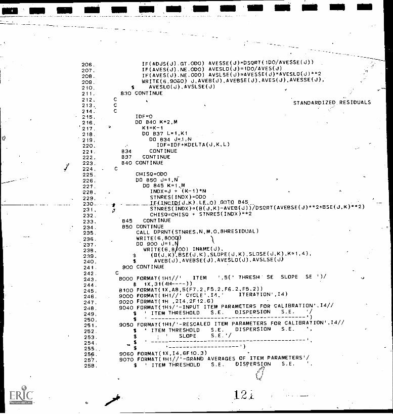
ma ow um so Ns Ns

206. IF(ADdS(A.GT.000) 4VESSE(J)=DSORT(1DO/4VESSE(0)207. IF(AVES(J).NE.ODO) AVESLO(J)=1D0/4VES(J)208. IF(AVES(J).NE.ODO) AVSLSE(J)=AVESSE(J)*AVESLO(J)**2209. WRITE(6,9060) J,AVEB(J),AVEBSE(J),AVES(J),AVESSE(J),210. $ AVESLO(J),AVSLSE(J)211. 830 CONTINUE

,

212. C

213, C ,STANDARDIZED RESIDUALS

214. C215. IDF=0216. DO 840 K=2,M217. u K1=K-1218. DO 837 L=1,K1219. DO 834 J=1,N220. IDF=IDF+KDELTA(U,K,L)221. 834 CONTINUE222. 837 CONTINUE223. 840 CONTINUE224. . C

225. CHISQ=ODO226. DO 850 J=1,W227. DO 845 K=1,M28. INDX=0 + (K-1)*N229. STNRES(INDX)=0D0

_.LECINCIDAJ,K).LE.0) GOTO 845231. 0 STNRES(INDX)=(B(J,K)-AVEB(J))/DSORT(AVEBSE(J)**2+BSE(J,K)**2)232. CHISO=CHISO + STNRES(INDX)**2233. 845 CONTINUE234. 850 CONTINUE235. CALL DPRNT(STNRES,N,M,0,8HRESIDUAL)236. WRITE(6,800 )

237. DO 900 J=1,238. WRITE(6,8 00) INAME(J),239. $ (8(J,K),BSE(J,K),SLOPE(J,K),SLOSE(U,K),K=1,4),240. $ AVEB(J),AVEBSE(J),AVESLO(J),AVSLSE(J)241. 900 CONTINUE242. C

243. 8000 FORMAT(1H1// ITEM ',5(' THRESH SE SLOPE SE ')/

244. $ 1X,31(4H----))245. 8100 FORMAT(1X,A8,5(F7.2,F5.2,F6.2,F5.2))246. 9000 FORMAT(1H1//' CYCLE',I4,' ITERATION',I4)

247. 9020 FORMAT(1H ,2I4,2F12.6)248. 9040 FORMAT(1H1P-INPUT ITEM PARAMETERS FOR CALIBRATION',I4//

249. $ ' ITEM THRESHOLD S.E. DISPERSION S.E.

250. $

251. 9050 FORM4T(1H1P-RESCALED ITEM PARAMETERS FOR CALIBR4TION',I4//

252. $ ' ITEM THRESHOLD S.E. DISPERSION S.E.

253. $ ' SLOPE S.E.'/

254. $ .

.

255. $

256. 9060 FORMAT(1X,I4,6F10.3) .

257. 9070 FORMAT(1H1//'-GRAND AVERAGES OF ITEM PARAMETERS'/258. $ ' ITEM THRESHOLD S.E. DISPERSION S.E.

S'',?

, ty,

1 2

IMO OM MI 1111111 111. MI 111111 4

259.260.261.262.26'3.

264.

SLOPE S.E.'/$ '

)

RETURNENDSUBROUTINE WEIGHT(KDELTA,RSCSLO,SE,W)

265. IMPLICIT REAL*8 (A-H2O-Z)266. REAL*8 INAME(20)267. COMMON/PARCOM/INAME,ACRIT,N,M,NM,METHOD,M1,NP,NTRIS,NTRIL,268. 1DIAG,MAXITR269. DIMENSION KDELTA,(20,4,4),RSCSLO(4),SE(20,4),W(20,4,4)270.271. DO 400 K=1,M272. K1=K-1273. .00 300 L=1,K1274. DO 200 J=1,N275. W(J,K,L)=000276. IF(KDELTA(J,K,L).LE.0) GOTO 100 .

277. W(J,K,L)=1DOMRSC5LO(K)*..SE(J,K))**2+(R5C5LO(L)*5E(J,L))**2)278. 100279. 200 CONTINUE280. 300 CONTINUE281. 400 CONTINUE282. IF(IDIAG.LT.2) G0T0570283. DO 570 J=1,N284. WRITE(6,6000) J,(L,L=1,M)285. DO 565 K=1,M286. WRITE(6,6100)(K,(W(J,K,L),L=1,M))287. 565 CONTINUE288. , 6000 FORMAT('-WEIGHT'MATRIX, ITEM',I4,10I10)289. 6100 FORMAT(12X,4X,I10,10F10.4)290. 570 CONTINUE291. C

292.

0

RETURN293. END294. SUBROUTINE FUNCT(RSCSLO,RSCINT,B,S,WB,WS,CHISQ)295.296. C COMPUTE CHI-SQUARE

297.298. IMPLICIT REAL*8 (A-H,Q-Z)299. REAL*8 INAMEc20)300. COMMON/PARCOM/INAME,ACRIT,N,M,NM,METHOO,M1,NP,NTRIS,NTRIL,301. IbIAG,MAXITR302. DIMENSION RSCSLO(4),RSCINT(4),B(20:4),S(20,4),303. $ WB(20,4,4),WS(20,4.4)304.305. CHISQ=000306. DO 500 K=1,M307. K1=K-1

,308. DO 400 L=1,K1309% IF(Kl.LE.0) GOTO 400310. DO 300 J=1,N311. IF(WB(J,K,L).LE.000) GOTO 300

12x:

312. CHISQ=CHISQ + (RSCSLO(K)*B(J,K) + RSCINT(K)313. -RSCSLO(L)*B(J,L) RSCINT(L))**2 * WB(J,K,L)

314. IF(METHOD.LT.2) GOTO 300315. CHISQ=CHISQ + (RSCSLO(K)*S(J,K)316. -RSCSLO(L)*S(J,L))**2 * WS(J,K,L)

317. 300 CONTINUE318. 400 CONTINUE319. 500 CONTINUE320. RETURN321. END322. SUBROUTINE FIRST(B,BSE,S,SSE,RSCSLO,RSCINT,WB,WS,FDRV)323. IMPLICIT REAL*8 (A-H2O-Z)324. REAL*8 INAME(20)325. COMMON/PARCOM/INAME,ACRIT,N,M,NM,METHOD,M1,NP,NTRIS,NTRIL,326. IDIAG,MAXITR327. DIMENSION.B(20,4),S(20,4),BSE(20,4),SSE(20,4),PSCSLO(4),RSCINT(4),328. $ WB(20,4,4),WS(20,4,4),FDRV(6)329.330. C FIRST DERIVS OF SLOPES

331.332. DO 190 K=2,M333. KX=K-1334. FDRV(KK)=0D0335. DO 170 J=1,N336. DO 150 L=1,M337. IF(L.EQ.K .0R. WB(U,K,L).LE.000) GOTO 150338. FDRV(KK)=FDRV(KK$ + WB(J,K,L)*339. (RSCSL0(K)*B(J,K)**2 RSCSLO(L)*B(J,K)*B(J,L)

340. + RSCINT(K)*B(J,K) RSCINT(L)*B(J,K))

341. IF(METHOD.LT.2) GOTO 150342. FDRV(KK)=FDPV(KK) + WS(J,K,L)*343. (RSCSLO(K)*S(J,K)**2 RSCSLO(L)*S(J,K)*S(J,L))

344. 150 CONTINUE345. 170 CONTINUE346. FDRV(KK)= FDRV(KK) 2D0

347. 190 CONTINUE348.349. C FIRST DERIVS OF INTRCPS

350.351. DO 290 K=2,M352. KK=M1 + (K-1)353. FDRV(KK)=000354. DO 270 J=1,N355. DO 250 L=1,M356. IF(L.EQ.K .0R. WB(U,K,L).LE..000) GOTO 250

357. FDRV(KK)=FDPV(KK) + WB(J,K,L)*

358. (RSCSLO(K)*B(J,K) - PSCSLOW*B(J,L)359. + RSCINT(K) RSCINT(L))

360. 250 CONTINUE361. 270 CONTINUE'362. FORV(KK)= FDRV.(KK) * 200 V

363. 290 CONTINUE /

364. IF(IDI6G.GT.0) CALL DPRNT(FDR\171,NP,0,8HFDPV )

or we am lie am au am um ow

365.366. RETURN367. END,

368. SUBROUTINE SECOND(B,BSE,S,SSE,RSCSLO,RSCINT,WB,WS,SDRV)369. IMPLICIT REAL*8 (A-H2O-Z)370. REAL*8 INAME(20)371. COMMON/PARCOM/INAME,ACRIT,N,M,NM,METHOD,M1,NP,NTRIS,NTRIL,372. $, 4DIAG,MAXITR373. DIMENSION B(20,4),5(20,4),BSE(20,4),SSE(20,4),RSCSLO(4),RSCINT(4),374. $ WB(20,4,4),WS(20,4,4),SDRV(21),SDRVA(6),375. $ SDRVB(9),SDRVC(6)376.377. C SLOPE DOUBLE DERIVS

37.8.

379. INDX=0380. DO 190 K=2,M381. INDX=INDX + (K-1)382. SDRVA(INDX)=0D0383. DO 170 J=1,N384. SUMWB=ODO,385. SUMWS=ODO386. DO 150 L=1,M387. IF(L.E0.K .0R. WB(J,K,L).LE.ODO) GOTO 150388. SUMWB=SUMWB + WB(J,K,L)389. SUMWS= SUMWS + WS(J,K,L)390. 150 CONTINUE391. SDRVA(INDX)=SDRVA(INDX)+ SUMWB*B(J,K)**2392. IF(METHOD.GE.2)393. SDRVA(INDX)=SDRVA(INDX) + SUMWS*S(J,K)**2

394. 170 CONTINUE395. SDRVA(INDX)=SDRVA(INDX) * 200396. 19,0 CONTINUE397.398. C SLOPE CROSS DERIVS

399.400. INDX=0401. DO 290 K=2,M402. DO 270 L=2,K403. INDX=INDX+1404. IF(L.EQ.K .0R. WB(J,K,L).LE.ODO) GOTO 270405. SDRVA(INDY) = ODO406. DO 250 J=1,N407. SDRVA(INDX)=SDRVA(INDX) + B(J,K)*B(J,L)*WB(J,K,L)

408. IF(METHOD.LT.2) GOTO 250409. SDRVA(INDX)=SDRVA(INDX) + S(J,K)*S(J,L)*WS(J,K,L)

410. 250 CONTINUE411. SDRVA(INDX) = SDRVA(INDX) * 200

412. 270 CONTINUE413. 290 CONTINUE414. , C415. C

SLOPE*INTRCP CROSS DERIVS,

416. C SAME CALIBRATION

417.

1 2 -;

cr

MO MI NM MN MN ION --1100 MN MI

418. DO 390 K=2,M419. KK=K-1420. INDX=(KK-1)*M1 + KK421. SDRVB(INDX)=0D0422. DO 370 J=1,N423. SUMWB = ODO424. DO 350 L=1,M425. IF(L.E0,K .0R. WB(d,K,L).LE.ODO) GOTO 350426. SUMWB=SUMWB + WB(J,K,L)427. 350 CONTINUE428. SDRVB(INDX)=SDRVB(INDX) + B(J,K)*SUMWB429. 370 CONTINUE430. ' SDRVB(INDX) = SDRVB(INDX) * 2D0431. 390 CONTINUE432.433. C SLOPE*INTRCP CROSS DER4VS,

434. C DIFFERENT CALIBRATIONS

435.436. INDX=0437. DO 490 K=2,M438. DO 470 L=2,M439. INDX=INDX+1440. IF(K.EQ.*6.) GOTO 470

441. SDRVB(INDX)=0D0442: DO 450 J=1,N443: SDRVB(INDX)=SDRVB(INDX) B(J,K)*WB(u,K,L)

444. 450 CONTINUE445, SDRVB(INDX) = SDRVB(INDX) * 2D0

446. 470 CONTINUE447. 490 CONTINUE448.449. C INTRCP DOUBLE DERIVS

450.451. INDX=0452. DO 590 K=2,M453. .INDX=INOX + (K-1)454. SORVC(INDX) = ODO455. DO 570 J=1,N456. DO 550 L=1,M457. IF(L.EQ.K .0R. WB(J,K,L).LE.ODO) GOTO 550458. SORVC(INDX) = SDRVC(INDX) + WB(J,K,L)

459. 550 CONTINUE460. 570 CONTINUE461. SORVC(INDX) = SDRVC(INDX) * 2D0462. 590 CONTINUE463.464. C INTRCP CROSS DERIVS

465.466. INDX=0467. DO 690 K=2,M 4

468. DO 670 L=2,K469. INOX=INDX + 1

470. IF(L.EQ.K :OR. WB(J,K,L):LE:ODO) GOTO 670

MI NM mom- -maw NI

471. SDRVC(INDX) = ODO472. DO 650 J=1,N473. SDRVC(INDX) = SDRVC(INDX) + WB(J,K,L)474. 650 CoNTINUE475. SDRVC(INDX) = SDRVC(INDX) * 2D0476. -670 CONTINUE477. 690 CONTINUE478.479. CALL ADORC(SDRVA,SDRVB,SDRVC,SDRV,M1,M1)480. IF(IDIAG.GT.0) CALL PpRNT(SDRV,Np,NP,1,8HsDRV481. RETURN482. END483. //Go.SYSIN DD *484. &INPUT N=17,M=4,METHOD=3,MAXITR=20,INAME=485. '5-A45532',486. '5-841532',487. '5-841732',488. '5-831732',489. '5-N00002,490. '5-811008',491. '5-A71043',492. '5-A21022',493. '5-832632',494. '5-K30004',495. '5-K10010',496. '5-833232',497. '5-G43009',498. '5-H12025',499. '5-G20001',500. '5-1<51020',501. '5-A21032',502. &END503. (I2,11,4F8.3)504. 41 3.046505. 51 -1.687506. 61 .185507. 81 .413

508. 91 2.681509. 101 1.107510. 111 3.756511. 121 :227

512. 131 1.923513. 52 -3.460514. 62 -3.010515. 102 .810516. 112 3.590517. 142', .700518. 162 -.150519. 13 -1.511520. 23 -.413521. 43 -.490522. 53 -3_420523. 63 -2.540

.360 5.263 .281

.360 5.000 .750,220 6.250 .781.160 4.000 .480.320 5.556 .926.270 10.000 2.000.440 5.263 .831

.220 6.667 , .889

.280 7.143 1.020

.610 5.000 .750

.720 10.000 2.000

.290 7.692 1.183

.610 5.556 .926

.290 7.692 1.183

.210 4.762 .680

.205 2.857 .335

.210 6.061 .882

.195 5.348 .744

.478 4.115 .559

.360 4.184 .543

1 26

NIB ION- MN MI MI III MI IIMI

524. 73 -1.378 .231 4.065 .512

525. 83 -1.319 .194 3.040 .351

526. 103 -2.325 .357 4.717 .623

527. 64 -5.283 .968 6.944 1.206

528. 84, -2.657 .454 5.155 .797

529. 114 .79? .260 6.329 1.001

530. 144 -2.084 .397 6.289 .989

531. 154 2.233 .338 5.464 .836

532. 174 1.533 .324 6.667 1.067

12

APPENDIX D,

COMMENTS ON NAEP PUBLIC-USE DATA TAPES

1 9 a

COMMENTS ON NAEP PUBLIC-USE DATA TAPES

Due to the quantity of information provided, the NAEP tapes

were in general cumbersome to work with. The documentation for

the 1977/1978 and change item tapes can only be described as

excellent, comprehensive in scope and accurate in detail. The

files comprising the tapes were well-organized, the information

about variable locations as well as that contained in the value

labels of the accompanying SPSS files was invaluable, and the

classification of items contained in the appendices greatly

facilitated the construction of our scales. In comparison, the

1972/1973 tape was more difficult to work with, the organization

and contents of the tape less readily understood.

A few minor difficulties that we encountered bear mentioning.

The difference between the "no response" and "missing values"

classifications of item responses is unclear from the documenta-

tion. The fact that in school and out of school 17 year olds are

assigned different values for the region variable proved to be a

source of temporary confusion.

Data for items which were supposed to .be invariant across two

or more age/year zombinations, according to the documentation

provided, occasionally did,not seem right. As an example, Item

5-832632 appeared in,both the 13-year old and 17-year old instru-

ments in 1977/78 as T1020 and S0921 respectiVely.. Proportions of

cpr=rect response however, .suggested the item to be,exteremly more

difficult for 17-year Olds,than 13-year,o1ds, atrend strongly

contradicting evidence from every other item linkirig these two age

years. It is likely that data for thc 17-year olds is in error

here. Similar problems arose for items 5-A71043 and 5-N00002.

Such questionable item/age/year data combinations were omitted in

our computations.

3