DOCUMENT

DE TRAVAIL

N° 518

DIRECTION GÉNÉRALE DES ÉTUDES ET DES RELATIONS INTERNATIONALES

OPTIONS EMBEDDED IN ECB TARGETED

REFINANCING OPERATIONS

Jean-Paul Renne

October 2014

DIRECTION GÉNÉRALE DES ÉTUDES ET DES RELATIONS INTERNATIONALES

OPTIONS EMBEDDED IN ECB TARGETED

REFINANCING OPERATIONS

Jean-Paul Renne

October 2014

Les Documents de travail reflètent les idées personnelles de leurs auteurs et n'expriment pas nécessairement la position de la Banque de France. Ce document est disponible sur le site internet de la Banque de France « www.banque-france.fr ». Working Papers reflect the opinions of the authors and do not necessarily express the views of the Banque de France. This document is available on the Banque de France Website “www.banque-france.fr”.

Options Embedded in ECB TargetedRefinancing Operations

Jean-Paul Renne∗

∗Banque de France; e-mail: jeanpaul.renne@banque-france.fr. This work has benefited from stimulatingdiscussions with Morten Bech, Ben Craig, Alain Monfort and Miklos Vari. I thank seminar participants atBanque de France for their comments. This paper expresses the views of the author; they do not necessarilyreflect those of the Banque de France.

.

Abstract: In June 2014, the European Central Bank (ECB) announced the implementationof new refinancing operations aimed at supporting bank lending to the non-financial privatesector. This paper exhibits and prices options embedded in these Targeted Longer-TermRefinancing Operations. In particular, it shows how these options participate to the incentivemechanisms at play in these operations. Quantitative results point to substantial gains –forparticipating banks– attached to the satisfaction of lending conditions defined by the scheme.

JEL Codes: E43, E52, E58.

Keywords: unconventional monetary policy, option pricing, TLTRO.

Résumé: En juin 2014, la Banque Centrale Européenne a annoncé la mise en place d’unnouveau type d’opérations de refinancement visant à stimuler les prêts bancaires au secteurprivé non-financier: les Targeted Longer-Term Refinancing Operations. Cet article met enlumière, puis valorise, des options incluses dans ces opérations. En particulier, il est mon-tré que ces options participent aux mécanismes incitatifs à l’oeuvre dans ces opérations.L’analyse quantitative suggère que les conditions de financement offertes par les TLTROssont particluièrement favorables pour les banques qui satisfont la contrainte de prêt définiedans le cadre du programme.

Codes JEL: E43, E52, E58.

Mots-Clés: politique monétaire non-conventionnelle, valorisation d’options, TLTRO.

Non-technical summary

The global financial turmoil incepted in 2007 and its implications on economic activity

have triggered unprecedented responses from major central banks. Some of these measures

specifically aim at supporting a continued provision of credit to the non-financial private

sector, that is to address potential impairments of the bank lending channel. The Targeted

Longer-Term Refinancing Operations (TLTROs), announced by the ECB in June 2014, fall

in that category.

The weakness of bank lending reflects a range of factors, but one major determinant is

the price that banks have to pay for funds. To be successful, funding-for-lending measures

have (a) to offer an attractive pricing and (b) to entail mechanisms incentivizing banks to

effectively lend to the economy. With this in mind, this paper examines TLTROs funding

conditions. It shows in particular that some options, embedded in TLTROs, have to be

taken into account when assessing the potential of these operations to meet objectives (a)

and (b). One of those options pertains to the possibility, for those banks fulfilling a lending

condition defined in the scheme, to pay back their loans before September 2018, which is

the maturity dates of TLTROs. Another option relates to the possibility, for participating

banks to borrow in the future at a rate indexed on the then-prevailing policy rates.

A specificity of these options is that their payoffs depend on future policy rates –as

opposed to market rates–. Since such options are not traded on financial markets, their

assessment has to be model-based. To that purpose, we use the model proposed in a com-

panion paper (Renne (2014)). This models explicitly incorporates policy rates and features

closed-form formulas for interest-rate options, making it appropriate to the present analysis.

The results suggest that those banks fulfilling the lending condition can expect to get funding

costs 5 to 10 basis points lower than those resulting from rolling over one-week central-bank

loans.

Introduction

1 Introduction

The global financial turmoil incepted in 2007 and its implications on economic activity

have triggered unprecedented responses from major central banks. Monetary authorities

have cut policy rates aggressively and adopted so-called unconventional monetary policies.1

Some of these measures specifically aim at supporting a continued provision of credit to the

non-financial private sector, that is to address potential impairments of the bank lending

channel.2 The Targeted Longer-Term Refinancing Operations (TLTROs) fall in that cate-

gory. Announced on 5 June 2014 by the Governing Council of the ECB, these measures aim

to "support bank lending to households and non-financial corporations, excluding loans to

households for house purchase."

This paper aims at quantifying the attractiveness of TLTROs. While the funding condi-

tions offered through TLTROs have been deemed to be "attractive" by market participants,

policymakers and medias alike, we are not aware of other quantitative studies of this aspect

at the time of writing.

The weakness of bank lending reflects a range of factors, but one major determinant is

the price that banks have to pay for funds. To be successful, funding-for-lending measures

have (a) to offer an attractive pricing and (b) to entail mechanisms incentivizing banks to

effectively lend to the economy. With this in mind, this paper examines TLTROs funding

conditions. It shows in particular that some options, embedded in TLTROs, have to be

taken into account when assessing the potential of these operations to meet objectives (a)

and (b). One of those options pertains to the possibility, for those banks fulfilling a lending1See, among many others, Borio and Disyatat (2010), Bowdler and Radia (2012), Trichet (2013) and

Gambacorta, Hofmann, and Peersman (2014). For a focus on how ECB intermediation has expanded duringthe crisis period, see Giannone, Lenza, Pill, and Reichlin (2010).

2Indeed, there is evidence that credit supply conditions have become more important for the transmissionof monetary policy than before the financial crisis, see e.g. Gambacorta and Marques-Ibanez (2011) orCappiello, Kadareja, Kok Sorensen, and Protopapa (2010). Specific examples of such measures includeschemes operated by the Bank of England ("Funding for Lending", see Churm, Radia, Leake, Srinivasan,and Whisker (2012)), the Central Bank of Hungary ("Funding for Growth Scheme") and the Bank of Japan("Fund-Provisioning Measure to Stimulate Bank Lending").

2

The TLTROs

condition defined in the scheme, to pay back their loans before September 2018, which is

the maturity dates of TLTROs. Another option relates to the possibility, for participating

banks to borrow in the future at a rate indexed on the then-prevailing policy rates.

A specificity of these options is that their payoffs depend on future policy rates –as

opposed to market rates–. Since such options are not traded on financial markets, their

assessment has to be model-based. To that purpose, we use the model proposed by Renne

(2014). This models explicitly incorporates policy rates and features closed-form formulas

for interest-rate options, making it appropriate to the present analysis. The results suggest

that those banks fulfilling the lending condition can expect to get funding costs 5 to 10 basis

points lower than those resulting from rolling over one-week central-bank loans.

The remaining of this paper is organized as follows. Section 2 pesents the TLTRO scheme.

Section 3 proposes an assessment of the TLTRO funding conditions and Section 4 concludes.

2 The TLTROs

The modalities of the TLTROs are presented in European Central Bank (2014); an exhaustive

description of the scheme is given by Governing Council of the ECB (2014). The different

TLTRO steps are represented in Figure 1. A series of TLTROs will be conducted between

September 2014 and June 2016. The interest rate of these operations will be fixed over the

life of the operation; the interest rate will be the MRO rate prevailing at the time of take-up,

plus a fixed spread of 10 basis points. For instance, the MRO being of 5 bps in fall 2014,

the rate of the first two TLTROs is 15 bps.

The amounts banks will be able to borrow during these operations are capped in the

following way:

• For the first two operations (September and December 2014), each bank will be able to

borrow up to 7% of the amount outstanding on 30 April 2014 of eligible loans granted

3

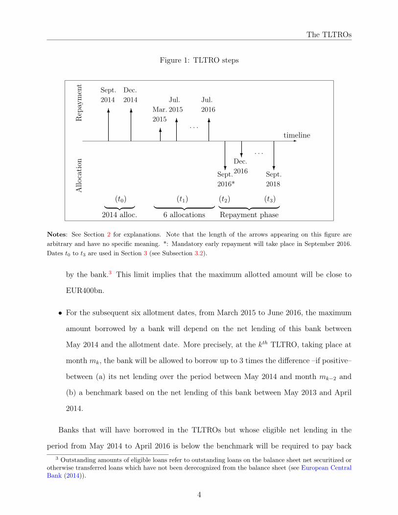
The TLTROs

Figure 1: TLTRO steps

-timeline

Allo

cation

Repay

ment

6

2014Sept.

6

2014Dec.

6

2015Mar.

6

2015Jul.

. . . 6

2016Jul.

?Sept.2016*

Dec.2016

?

Sept.2018

?

. . .

(t0) (t1) (t2) (t3)︸ ︷︷ ︸2014 alloc.

︸ ︷︷ ︸6 allocations

︸ ︷︷ ︸Repayment phase

Notes: See Section 2 for explanations. Note that the length of the arrows appearing on this figure arearbitrary and have no specific meaning. *: Mandatory early repayment will take place in September 2016.Dates t0 to t3 are used in Section 3 (see Subsection 3.2).

by the bank.3 This limit implies that the maximum allotted amount will be close to

EUR400bn.

• For the subsequent six allotment dates, from March 2015 to June 2016, the maximum

amount borrowed by a bank will depend on the net lending of this bank between

May 2014 and the allotment date. More precisely, at the kth TLTRO, taking place at

month mk, the bank will be allowed to borrow up to 3 times the difference –if positive–

between (a) its net lending over the period between May 2014 and month mk−2 and

(b) a benchmark based on the net lending of this bank between May 2013 and April

2014.

Banks that will have borrowed in the TLTROs but whose eligible net lending in the

period from May 2014 to April 2016 is below the benchmark will be required to pay back3 Outstanding amounts of eligible loans refer to outstanding loans on the balance sheet net securitized or

otherwise transferred loans which have not been derecognized from the balance sheet (see European CentralBank (2014)).

4

TLTRO pricing

their borrowings in September 2016. This condition will refer to as Condition C in the sequel

of this note. Moreover, the banks that do (do not) satisfy this condition will be referred to

as performing (nonperforming) banks.

Condition C. This condition is satisfied by a given bank if its net lending in the period from

May 2014 to April 2016 is equal to –or above– its benchmark.

3 TLTRO pricing

Banks will participate to the TLTRO if these operations are attractive enough for banks.

An important ingredient of TLTRO attractiveness pertains to the funding conditions offered

by these operations. Subsection 3.1 presents a rough assessment of TLTRO funding condi-

tions. Subsection 3.2 introduces a stylized view of the TLTRO framework. Subsection 3.3

formulates TLTRO features as options. Subsection 3.4 values these options and Subsection

3.5 exploits this valuation exercise to build a comprehensive assessment of TLTRO funding

conditions.

3.1 At first sight

A first gauge of TLTROs’ attractiveness is obtained by comparing the rate of the initial

TLTROs with alternative funding costs for banks. However, finding a relevant benchmark

rate is not straightforward for several reasons. First, banks do not constitute an homogenous

group and funding conditions diverge across them. Second, TLTROs are secured operations

and the type of collateral accepted by the Eurosystem is wider than the one accepted in

standard market repo operations.4 This latter point implies that private-market repo rates

cannot be directly compared to TLTROs’ ones.4The importance of the collateral framework is e.g. demonstrated by Eisenschmidt, Hirsch, and Linzert

(2009). For a recent survey on central-bank collateral frameworks and practices, see Bank for InternationalSettlements (2013).

5

TLTRO pricing

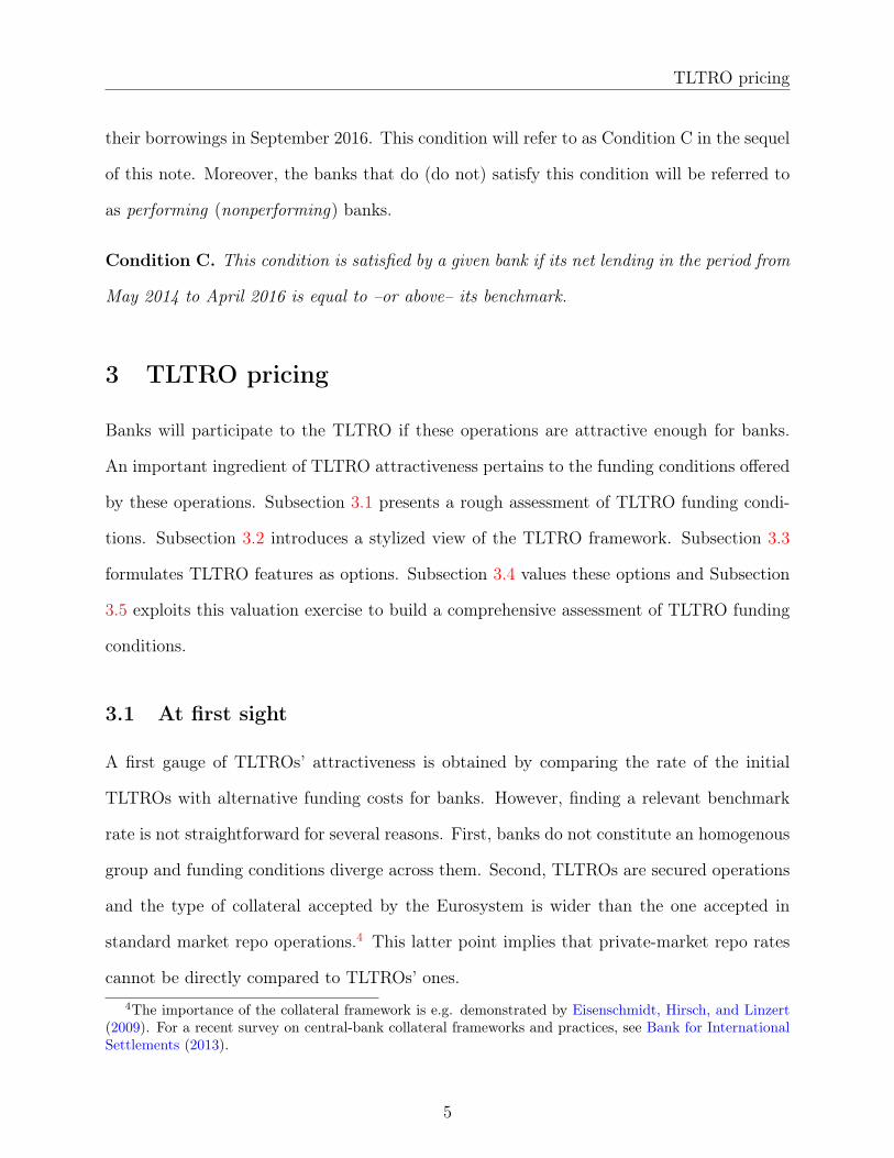
While it is difficult to find private market operations similar to TLTROs, it is nevertheless

instructive to compare TLTRO conditions with the funding costs associated with different

borrowing operations.5 In that preliminary exercise, we focus on 4-year yields, which is the

longest maturity of TLTRO operations. We consider two "extreme" benchmarks.

The first corresponds to a (synthetic) 4-year general-collateral repurchase agreement.

Repos for such long maturities do not exist; they can however be synthesized and the resulting

rates can be proxied by Overnight Indexed Swaps (OIS) rates.6 Since the class of collateral

eligible to such repo is much narrower than for Eurosystem refi operations, the rate of such

an operation is expected to be lower than the 4-year TLTRO one.

A second benchmark rate is that of unsecured borrowing, which we proxy by an average

of 4-year unsecured bond yields. These bonds constituting a non-collateralized funding, this

second benchmark rate is expected to be higher than TLTRO rates. Figure 2 displays the

fluctuations of the two benchmark rates. It appears that the initial TLTRO rate (15 bps)

is close to the lower bound of the interval delineated by these two yields, pointing to the

attractiveness of TLTROs.

Assessing the values associated with the different collateralizations of these different fund-

ing operations (private-market repo, central-bank refinancing operations and unsecured-bond

issuances) is beyond the scope of the present paper. The methodology developed in the fol-

lowing rather aims at comparing TLTRO funding costs with alternative central-bank funding

operations n order to bypass problems stemming from differences in collateralizations.

5To that respect, there is evidence that ECB LTROs are seen by banks as partial substitutes to alternativesfunding sources (see e.g. Reuters (2014)).

6An OIS is an interest rate swap whose floating leg is tied to an overnight interbank rate (the EONIAin the euro-area case), compounded over a specified term. A 4-year repo can be synthetically obtained byrolling a shorter-term repo and to enter in a 4-year OIS contract where the bank pays the fixed rate. Thisresults in a synthetic collateralized funding where the bank pays the 4-year fixed rate (the short-term reporates paid by the bank being approximately covered by the capitalized EONIA rates resulting from the 4-yearOIS contract).

6

TLTRO pricing

Figure 2: Proxies of 4-year funding costs of banks

2013 2014

0.0

0.5

1.0

1.5

2.0

2.5

3.0

3.5

Ann

ualiz

ed in

tere

st r

ate

(in %

)

4−year OIS (proxy of 4−year secured funding cost)4−year unsecured bond yield (A−rated banks)15 bps TLTRO rate (initial allowances)

Notes: This figure displays two proxies of 4-year bank lending rates. The Overnight Indexed Swap (OIS)rate is a proxy of the rate of a synthetic repo where the collateral is the one accepted in general-collateralprivate-markets repurchase agreements. The dashed line is an average of the yields-to-maturity of 4-yearbonds issued by A-rated European banks (Source: Bloomberg). Time ranges form 3 December 2013 to 1October 2014.

3.2 Stylizing the TLTRO scheme

For expository and computational convenience, let us simplify the TLTRO framework and

summarize the different steps of the schemes as follows:

• t0 : Initial TLTRO allocations [2014];

• t1 : Additional TLTROs [March 2015 to June 2016];

• t2 : Early repayment [2016] (compulsory for non-performing banks);

• t3 : Maturity of TLTROs [2018].

As stressed in Subsection 3.1, it is difficult to find a private-market source of funding

that is close enough to he TLTRO to serve as a proper benchmark. Nevertheless, there is a

basic funding strategy that a bank can follow as an alternative to participating to TLTROs:

this strategy simply consists in recurrently participating to the main refinancing operations

7

TLTRO pricing

(MRO) of the Eurosystem, for which banks get one-week funding at a rate denoted byMROt.

The collateral required by those operations is the same as the TLTRO one. Hence, this

strategy appears to be a natural and relevant benchmark for TLTRO operations. However,

from a given date, the cost of the roll-over strategy is unknown since it depends on future

MRO rates. Formally, denoting by t∗ the termination date of this strategy, the date-t value

of the associated annualized interest-rate load is given by:

yt,t∗ =1

t∗ − tEt(MROt +MROt+1 + · · ·+MROt∗−1), (1)

where Et denotes the risk-neutral expectation based on all information available at date t.

The previous formula is actually the one that would be used to price swaps with floating-leg

cash-flows indexed to MRO rates; but such swaps do not trade.7 Notwithstanding, estimates

of the previous rates can be derived from an appropriate interest-rate model (Subsection

3.4).

3.3 Concept of TLTRO-embedded options

The present subsection shows that some TLTRO features can be expressed in terms of options

implicitly given to banks. Specifically, we exhibit three TLTRO-embedded options.

Let us consider a performing bank, which is a bank satisfying Condition C. It is tempting

to say that the funding cost attached to the initial TLTRO loans is of 15 bps. However, this

neglects the existence of a first option, which pertains to the possibility, for this bank, to

repay the loan at date t2. This bank will typically exercise this option if, at date t2, it expects7By contrast, a liquid contract indexed on future Fed Funds rates exist in the United States (see Gurkaynak

(2005), Carlson, Craig, and Melick (2005) or Gurkaynak, Sack, and Swanson (2007)), markets in most othercountries rely exclusively on their local-currency- denominated OIS market for hedging central bank policy.Note that these market instruments are different from OIS, whose floating legs are indexed to overnightinterbank rates (EONIA). Before October 2008, the EONIA were on average very close to the MRO rate butthis changed with the implementation of the fixed-rate full allotment policy of the Eurosystem. Since then,the EONIA have persistently evolved below the MRO rate, at the bottom of the so-called monetary-policy-rate corridor.

8

TLTRO pricing

a lower interest cost from a MRO roll-over strategy over the residual time-to-maturity of the

loan (i.e. between dates t2 and t3). That is, this bank will exercise this option at date t2 if

yt2,t3−t2 < 15 bps.

TLTRO-embedded Option 1. The fact that performing banks can –but are not obliged

to– repay TLTROs before maturity (t3) implies that TLTRO funding embeds options that

allow participating banks to benefit from potential future decreases in alternative funding

rates between repayment dates (t2) and the maturity of TLTROs (t3).

The payoff of this first option is represented in Figure 3. The same figure also shows

the payoff of a second option. The latter is very much related to the previous one; to some

extent, it can be seen as a rephrasing of Option 1. (Actually, instead of saying that this

second option is an option that performing banks have, one should rather say that it is

an option that non-performing banks do not have.) This option is nonetheless important

because it reflects the incentives banks have to perform. This option reads:

TLTRO-embedded Option 2. The fact that performing banks can go on their initial

TLTRO loans after 2016 (date t2) implies that TLTROs embed options that allow performing

banks –by contrast to non-performing banks– to be shielded against future potential increases

in alternative funding rates between repayment dates (t2) and the maturity of the TLTRO

operations (date t3).

Finally, banks that engage in outperforming Condition C acquire a third type of option.

The latter option pertains to the possibility, between March 2015 and June 2016 (date t1), to

obtain funding at MROt1 + 10 bps (up to a given threshold based on the difference between

its net lending and the benchmark, see Section 2). Figure 4 represents the date-t1 payoff

associated with Option 3.

9

TLTRO pricing

Figure 3: Payoffs of Options 1 & 2

-

Expected MRO ratebetween dates t2and t3 (yt2,t3)

6

15 bps

Payoffs (as of date t2)

@@@@@@@@

?

6

Payoff of Option 2(solid line − dashed line)

��

Payoff of Option 1(solid line)

Notes: Option 1: The black solid line is the payoff of Option 1. This payoff will materialize at date t2 (mid2016). At that date, performing banks –i.e. those that do have satisfied Condition C– have the possibilityto keep their initial TLTRO funding until maturity (date t3, 2018). They will do so if they expect the MROrate between t2 and t3 (this expectation is denoted by yt2,t3 , see Equation 1) to stay above the 15 bps theypay on TLTRO loans. Otherwise, they can choose to switch to MRO funding. This gives rise to the payoffof Option 1. Option 2: The payoff of Option 2 highlights the gains banks have to perform, i.e. to satisfyCondition C. Nonperforming banks are compelled to repay TLTRO loans at date t2. Hence, compared toperforming banks, they face a negative payoff when yt2,t3 is higher than 15 bps.

TLTRO-embedded Option 3. Banks that outperform their benchmark acquire the option

to get funding at a fixed rate of MROt1 + 10 bps at the TLTROs that will take place between

March 2015 and June 2016 (date t1). The maturity date of these loans is September 2018

(date t3).

3.4 Valuation of TLTRO-embedded options

Options 1 to 3 are not standard options. First, the underlying rates are MRO rates while

the payoffs of standard options are indexed on EURIBOR rates. Second, contrary to Option

10

TLTRO pricing

Figure 4: Payoff of Option 3

-

6

�������

MROt1 + 10 bps

Payoff (as of date t1)

Expected MRO ratebetween dates t1and t3 (yt1,t3)

Notes: At date t1 (March 2015 - June 2016), performing banks have the option to get additional TLTROfunding at MROt1 + 10 bps until the TLTRO maturity (date t3, 2018). Hence, Option 3 pays off if the rateof the alternative strategy (rolling over MRO fundings between dates t1 and t3, whose expected annualizedcost is yt1,t3) is above MROt1 + 10 bps.

1 and 2, Option 3 is not structured as a usual swaption8 in that the strike rate is not known

at the inception of the "contract", i.e. at date t0: indeed, Option 3 gives to its holder the

right to enter, in the future, i.e. at date t1, a swap whose fixed rate is MROt1 + 10 bps,

which is unknown as of date t0.

Pricing these options hence requires a specific setup. The model proposed by Renne

(2014) is relevant in this context. This model, whose broad lines are given in Appendix

A, relies on an original specification of the policy-rate dynamics. This model is actually

one of the very few term-structure models that explicitly incorporate policy rates, which

is required in the current context (notably to compute the MRO-swap yields of Equation

1). An advantage of this framework is that it offers analytical formulas for the valuation of

swaps, swaptions, caps and floors. As a consequence, it can easily be parameterized to fit

various market data. Once the model parameters are obtained, the model can further be

exploited in order to price other instruments. Typically, in the present case, the estimated8A swaption is an option granting its owner the right but not the obligation to enter into an underlying

swap in the future, the fixed rate of the swap being predetermined (at the date where the swaption iscontracted).

11

TLTRO pricing

model can be used to price Options 1, 2 and 3.

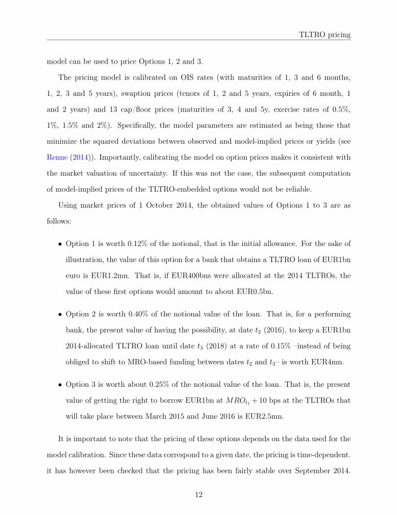
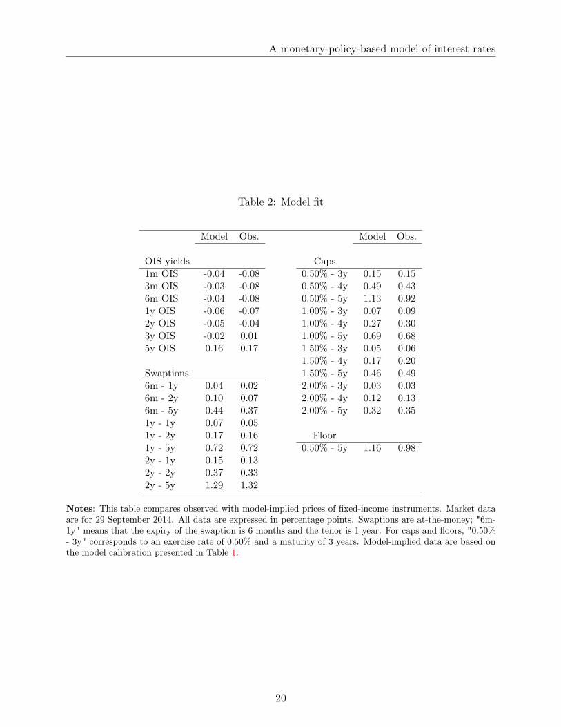
The pricing model is calibrated on OIS rates (with maturities of 1, 3 and 6 months,

1, 2, 3 and 5 years), swaption prices (tenors of 1, 2 and 5 years, expiries of 6 month, 1

and 2 years) and 13 cap/floor prices (maturities of 3, 4 and 5y, exercise rates of 0.5%,

1%, 1.5% and 2%). Specifically, the model parameters are estimated as being those that

minimize the squared deviations between observed and model-implied prices or yields (see

Renne (2014)). Importantly, calibrating the model on option prices makes it consistent with

the market valuation of uncertainty. If this was not the case, the subsequent computation

of model-implied prices of the TLTRO-embedded options would not be reliable.

Using market prices of 1 October 2014, the obtained values of Options 1 to 3 are as

follows:

• Option 1 is worth 0.12% of the notional, that is the initial allowance. For the sake of

illustration, the value of this option for a bank that obtains a TLTRO loan of EUR1bn

euro is EUR1.2mn. That is, if EUR400bns were allocated at the 2014 TLTROs, the

value of these first options would amount to about EUR0.5bn.

• Option 2 is worth 0.40% of the notional value of the loan. That is, for a performing

bank, the present value of having the possibility, at date t2 (2016), to keep a EUR1bn

2014-allocated TLTRO loan until date t3 (2018) at a rate of 0.15% –instead of being

obliged to shift to MRO-based funding between dates t2 and t3– is worth EUR4mn.

• Option 3 is worth about 0.25% of the notional value of the loan. That is, the present

value of getting the right to borrow EUR1bn at MROt1 + 10 bps at the TLTROs that

will take place between March 2015 and June 2016 is EUR2.5mn.

It is important to note that the pricing of these options depends on the data used for the

model calibration. Since these data correspond to a given date, the pricing is time-dependent.

it has however been checked that the pricing has been fairly stable over September 2014.

12

TLTRO pricing

Besides, while the calibrated model provides a fairly good fit of observed prices, the fit is

not perfect (see Appendix A). Therefore, these results should be interpreted with caution.

Nevertheless, different checks point to the robustness of the order of magnitude of reported

results.

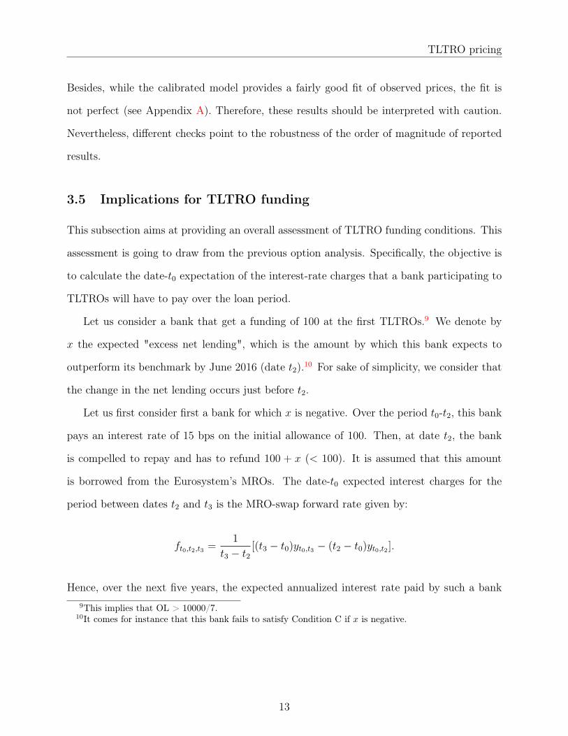
3.5 Implications for TLTRO funding

This subsection aims at providing an overall assessment of TLTRO funding conditions. This

assessment is going to draw from the previous option analysis. Specifically, the objective is

to calculate the date-t0 expectation of the interest-rate charges that a bank participating to

TLTROs will have to pay over the loan period.

Let us consider a bank that get a funding of 100 at the first TLTROs.9 We denote by

x the expected "excess net lending", which is the amount by which this bank expects to

outperform its benchmark by June 2016 (date t2).10 For sake of simplicity, we consider that

the change in the net lending occurs just before t2.

Let us first consider first a bank for which x is negative. Over the period t0-t2, this bank

pays an interest rate of 15 bps on the initial allowance of 100. Then, at date t2, the bank

is compelled to repay and has to refund 100 + x (< 100). It is assumed that this amount

is borrowed from the Eurosystem’s MROs. The date-t0 expected interest charges for the

period between dates t2 and t3 is the MRO-swap forward rate given by:

ft0,t2,t3 =1

t3 − t2[(t3 − t0)yt0,t3 − (t2 − t0)yt0,t2 ].

Hence, over the next five years, the expected annualized interest rate paid by such a bank9This implies that OL > 10000/7.

10It comes for instance that this bank fails to satisfy Condition C if x is negative.

13

TLTRO pricing

is:

(t2 − t0)100

(t2 − t0)100 + (t3 − t2)(100 + x)0.15% +

(t3 − t2)(100 + x)

(t2 − t0)100 + (t3 − t2)(100 + x)ft0,t2,t3 . (2)

Now, let us turn to a bank for which x ≥ 0. This bank benefits from Options 1 and 3. To

compute the expected interest cost faced by this bank, we take advantage of our options

pricing. Specifically, the date-t0 cost is computed as if the banks sold the options at date

t0, the proceeds of these sales being taken off the interest charges. Further, it is assumed

that, at the additional TLTROs of March 2015 to June 2016, the bank draws the fraction

θ ∈ [0, 1] of their maximum borrowing allowance. The average interest charge for this bank

is then given by:

(t3 − t0)100

(t3 − t0)100 + (t3 − t1)3θx

(0.15%− Opt1

t3 − t0

)+

(t3 − t1)3θx(t3 − t0)100 + (t3 − t1)3θx

(ft0,t1,t3 −

Opt3t3 − t1

). (3)

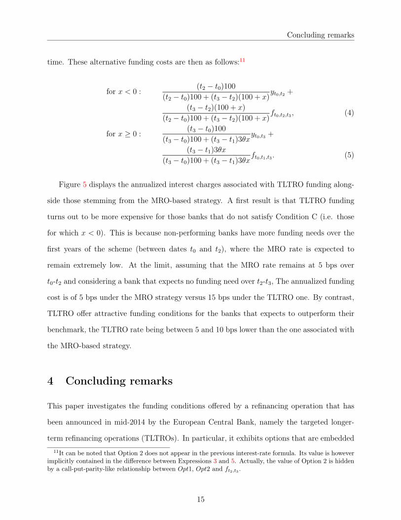
The expected cost of TLTRO funding can be compared to that stemming from a MRO-

based strategy, that is a funding strategy where banks get central-bank funding only through

weekly main refinancing operations. In order to get comparable rates, we compute the

expected costs associated with this alternative strategy using equivalent funding needs over

14

Concluding remarks

time. These alternative funding costs are then as follows:11

for x < 0 :(t2 − t0)100

(t2 − t0)100 + (t3 − t2)(100 + x)yt0,t2 +

(t3 − t2)(100 + x)

(t2 − t0)100 + (t3 − t2)(100 + x)ft0,t2,t3 , (4)

for x ≥ 0 :(t3 − t0)100

(t3 − t0)100 + (t3 − t1)3θxyt0,t3 +

(t3 − t1)3θx(t3 − t0)100 + (t3 − t1)3θx

ft0,t1,t3 . (5)

Figure 5 displays the annualized interest charges associated with TLTRO funding along-

side those stemming from the MRO-based strategy. A first result is that TLTRO funding

turns out to be more expensive for those banks that do not satisfy Condition C (i.e. those

for which x < 0). This is because non-performing banks have more funding needs over the

first years of the scheme (between dates t0 and t2), where the MRO rate is expected to

remain extremely low. At the limit, assuming that the MRO rate remains at 5 bps over

t0-t2 and considering a bank that expects no funding need over t2-t3, The annualized funding

cost is of 5 bps under the MRO strategy versus 15 bps under the TLTRO one. By contrast,

TLTRO offer attractive funding conditions for the banks that expects to outperform their

benchmark, the TLTRO rate being between 5 and 10 bps lower than the one associated with

the MRO-based strategy.

4 Concluding remarks

This paper investigates the funding conditions offered by a refinancing operation that has

been announced in mid-2014 by the European Central Bank, namely the targeted longer-

term refinancing operations (TLTROs). In particular, it exhibits options that are embedded11It can be noted that Option 2 does not appear in the previous interest-rate formula. Its value is however

implicitly contained in the difference between Expressions 3 and 5. Actually, the value of Option 2 is hiddenby a call-put-parity-like relationship between Opt1, Opt2 and ft2,t3 .

15

Concluding remarks

Figure 5: TLTROs vs. MROs – Expected annualized funding cost

−40 −20 0 20 40

0.10

0.15

0.20

0.25

0.30

θ = 0.3

Expected excess net lending (x), in % of initial allowance

Exp

ecte

d an

nual

ized

inte

rest

pay

men

t (in

%)

Funding strategy:

TLTROMRO Roll−over

−40 −20 0 20 40

0.10

0.15

0.20

0.25

0.30

θ = 1

Expected excess net lending (x), in % of initial allowance

Exp

ecte

d an

nual

ized

inte

rest

pay

men

t (in

%)

Notes: These plots the expected annualized funding costs associated with two strategies involving Eurosys-tem financing operations. For x < 0 (respectively x ≥ 0), the solid line corresponds to Expression 2 (resp.Expression 3). The dashed lines represent the expected annualized costs of a funding strategy whereby thebank gets its funding only through the weekly main refinancing operations (MROs) held by the Eurosystem(Expression 4 and 5). The horizontal gray line indicates the rate of the initial TLTROs (0.15%).

in the TLTROs and shows that these options are key to the incentive mechanisms at play

in these non-conventional monetary-policy measures.

It has to be stressed that the analysis developed in this paper solely focuses on pricing

aspects and does not provide an exhaustive view of all TLTROs’ pros and cons from the

banks’ point of view. In particular:

• When TLTRO funding conditions are compared to the ones expected from rolling over

short-term central-bank loans, it is implicitly assumed that the latter are going to

be fully allotted over the next four years; the ECB has however not committed to

maintaining its fixed-rate full-allotment (FRFA) policy in place over that horizon.12

• The long maturity for these loans is helpful to banks that are concerned about satisfying

regulations on net stable funding ratios (Whelan (2014)).12At the time of writing, the ECB has committed to operate refinancing operations under FRFA at least

until September 2016.

16

Concluding remarks

• Potential costs specifically associated with the fulfillment of the lending-related con-

ditionality involved in TLTRO operations are not taken into account in the present

analysis.13

13Costs could e.g. arise if, in order to satisfy this condition (Condition C the paper), it had to reduce itslending standards below their usual levels or to reduce its lending rates so as to meet a big enough creditdemand. Another form of potential costs relates to stigma effects (see Cecchetti (2009)), whereby a bankmay fear to be viewed as being in weak condition if it borrows a lot of money from the central bank.

17

A monetary-policy-based model of interest rates

A A monetary-policy-based model of interest rates

More details on the modeling approach can be found in Renne (2014).

Specification of the overnight interbank rate

In the model, the short-term rate is given by: rt = ∆′zt + ξt where zt is a selection vector

(i.e. full of zeros, except one entry that equals one), ∆ is a vector of possible values of the

MRO rate (that we set to 0.05%, 0.25%, 0.50% . . . , 10%) and where, conditionally to zt, ξt is

an i.i.d. random variable. Hence, the dynamics of the short-term rate is mainly driven by

that of the state vector zt.

The regimes (represented by zt)

In addition to indicating the level of the current policy rate, the state zt depends (a) on

the current monetary-policy phase that can be either "easing" (policy-rate cuts are expected

at next governing-council meeting), "tightening" (hikes are expected) or in "status quo"

(neither cuts nor hikes are likely) and (b) on the monetary-policy corridor functioning that

can be either "normal" (the overnight interbank rate is close to the middle of the corridor ≡

MRO rate) or "in excess-liquidity" (the overnight interbank rate stands substantially below

the MRO rate). Under a normal functioning of the corridor system (respectively under the

floor system), the conditional mean of ξt is 0 (resp. −δ).

Formally, we have: zt = zc,t � zm,t � zr,t, where zc,t is the selection vector of the corridor

regime (of dimension 2 × 1), zm,t is the selection vector of the monetary policy phase (of

dimension 3× 1) and zr,t is the selection vector of the policy rate (of dimension K × 1 if K

is the number of possible policy rates).

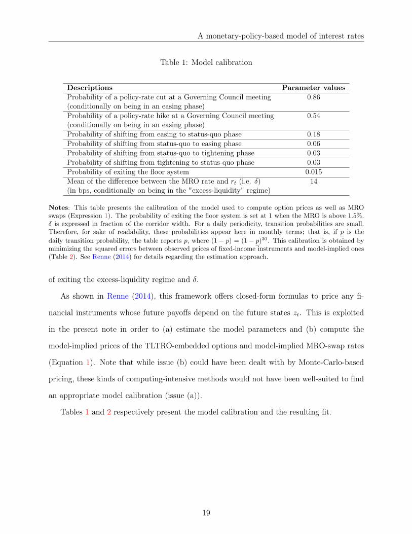
Dynamics of zt and model parameterization

The selection vector zt follows a Markovian process whose matrix of transition probabili-

ties is denoted by Π. This large matrix is parameterized by six parameters (see first six lines

in Table 1). Two additional parameters are required to calibrate the model: the probability

18

A monetary-policy-based model of interest rates

Table 1: Model calibration

Descriptions Parameter valuesProbability of a policy-rate cut at a Governing Council meeting 0.86(conditionally on being in an easing phase)Probability of a policy-rate hike at a Governing Council meeting 0.54(conditionally on being in an easing phase)Probability of shifting from easing to status-quo phase 0.18Probability of shifting from status-quo to easing phase 0.06Probability of shifting from status-quo to tightening phase 0.03Probability of shifting from tightening to status-quo phase 0.03Probability of exiting the floor system 0.015Mean of the difference between the MRO rate and rt (i.e. δ) 14(in bps, conditionally on being in the "excess-liquidity" regime)

Notes: This table presents the calibration of the model used to compute option prices as well as MROswaps (Expression 1). The probability of exiting the floor system is set at 1 when the MRO is above 1.5%.δ is expressed in fraction of the corridor width. For a daily periodicity, transition probabilities are small.Therefore, for sake of readability, these probabilities appear here in monthly terms; that is, if p is thedaily transition probability, the table reports p, where (1 − p) = (1 − p)30. This calibration is obtained byminimizing the squared errors between observed prices of fixed-income instruments and model-implied ones(Table 2). See Renne (2014) for details regarding the estimation approach.

of exiting the excess-liquidity regime and δ.

As shown in Renne (2014), this framework offers closed-form formulas to price any fi-

nancial instruments whose future payoffs depend on the future states zt. This is exploited

in the present note in order to (a) estimate the model parameters and (b) compute the

model-implied prices of the TLTRO-embedded options and model-implied MRO-swap rates

(Equation 1). Note that while issue (b) could have been dealt with by Monte-Carlo-based

pricing, these kinds of computing-intensive methods would not have been well-suited to find

an appropriate model calibration (issue (a)).

Tables 1 and 2 respectively present the model calibration and the resulting fit.

19

A monetary-policy-based model of interest rates

Table 2: Model fit

Model Obs. Model Obs.

OIS yields Caps1m OIS -0.04 -0.08 0.50% - 3y 0.15 0.153m OIS -0.03 -0.08 0.50% - 4y 0.49 0.436m OIS -0.04 -0.08 0.50% - 5y 1.13 0.921y OIS -0.06 -0.07 1.00% - 3y 0.07 0.092y OIS -0.05 -0.04 1.00% - 4y 0.27 0.303y OIS -0.02 0.01 1.00% - 5y 0.69 0.685y OIS 0.16 0.17 1.50% - 3y 0.05 0.06

1.50% - 4y 0.17 0.20Swaptions 1.50% - 5y 0.46 0.496m - 1y 0.04 0.02 2.00% - 3y 0.03 0.036m - 2y 0.10 0.07 2.00% - 4y 0.12 0.136m - 5y 0.44 0.37 2.00% - 5y 0.32 0.351y - 1y 0.07 0.051y - 2y 0.17 0.16 Floor1y - 5y 0.72 0.72 0.50% - 5y 1.16 0.982y - 1y 0.15 0.132y - 2y 0.37 0.332y - 5y 1.29 1.32

Notes: This table compares observed with model-implied prices of fixed-income instruments. Market dataare for 29 September 2014. All data are expressed in percentage points. Swaptions are at-the-money; "6m-1y" means that the expiry of the swaption is 6 months and the tenor is 1 year. For caps and floors, "0.50%- 3y" corresponds to an exercise rate of 0.50% and a maturity of 3 years. Model-implied data are based onthe model calibration presented in Table 1.

20

REFERENCES

References

Bank for International Settlements (2013). Central Bank Collateral Frameworks and Practices.

Report by a Study Group established by the Market Committe, BIS.

Borio, C. and P. Disyatat (2010, 09). Unconventional Monetary Policies: An Appraisal. Manchester

School 78 (s1), 53–89.

Bowdler, C. and A. Radia (2012, WINTER). Unconventional Monetary Policy: the Assessment.

Oxford Review of Economic Policy 28 (4), 603–621.

Cappiello, L., A. Kadareja, C. Kok Sorensen, and M. Protopapa (2010). Do Bank Loans and Credit

Standards have an Effect on Output? A Panel Approach for the euro area. ECB Working Paper

1150.

Carlson, J. B., B. R. Craig, and W. R. Melick (2005). Recovering Market Expectations of FOMC

Rate Changes with Options on Federal Funds Futures. Journal of Futures Markets 25 (12), 1203–

1242.

Cecchetti, S. G. (2009). Crisis and Responses: The Federal Reserve in the Early Stages of the

Financial Crisis. Journal of Economic Perspectives 23 (1), 51–75.

Churm, R., A. Radia, J. Leake, S. Srinivasan, and R. Whisker (2012). The Funding for Lending

Scheme. Bank of England Quarterly Bulletin 52 (4), 306–320.

Eisenschmidt, J., A. Hirsch, and T. Linzert (2009). Bidding Behaviour in the ECB’s Main Refi-

nancing Operations during the Financial Crisis. ECB Working Paper 1052, ECB.

European Central Bank (2014). Targeted Longer-Term Refinancing Operations: Updated Modali-

ties. ECB document, July 29, 2014, ECB.

Gambacorta, L., B. Hofmann, and G. Peersman (2014). The Effectiveness of Unconventional Mon-

etary Policy at the Zero Lower Bound: A Cross-Country Analysis. Journal of Money, Credit and

Banking 46 (4), 615–642.

21

REFERENCES

Gambacorta, L. and D. Marques-Ibanez (2011). The Bank Lending Channel: Lessons from the

Crisis. Economic Policy , 135–182.

Giannone, D., M. Lenza, H. Pill, and L. Reichlin (2010). Non-standard Monetary Policy Measures

and Monetary Developments. CEPR Discussion Paper 8125, CEPR.

Governing Council of the ECB (2014). Decision of the European Central Bank of 29 July 2014 on

Measures Relating to Targeted Longer-Term Refinancing Operations (ECB/2014/34). Official

Journal of the European Union L 258.

Gros, D., C. Alcidi, and A. Giovannini (2014). Targeted Longer-Term Refinancing Operations

(TLTROs): Will They Revitalise Credit in the Euro Area? Document Requested by the European

Parliament’s Committee on Economic and Monetary Affairs IP/A/ECON/2014-03.

Gurkaynak, R. S. (2005). Using Federal Funds Futures Contracts For Monetary Policy Analysis.

Finance and Economics Discussion Series 2005-29, Board of Governors of the Federal Reserve

System (U.S.).

Gurkaynak, R. S., B. T. Sack, and E. P. Swanson (2007). Market-Based Measures of Monetary

Policy Expectations. Journal of Business & Economic Statistics 25, 201–212.

Renne, J.-P. (2014). Fixed-Income Pricing in a Non-Linear Interest-Rate Model. Banque de France

Working Paper forthcoming, Banque de France.

Reuters (2014). TLTRO to Stall Bank Funding Plans. Reuters news, Fri Jul 25, 2014.

Trichet, J.-C. (2013). Unconventional Monetary Policy Measures: Principles-Conditions-Raison

d’Etre. International Journal of Central Banking 9 (1), 229–250.

Whelan, K. (2014). The ECB and Non-Standard Policies: Too Little Too Late? Document

was requested by the European Parliament’s Committee on Economic and Monetary Affairs

IP/A/ECON/2014-02.

22

Documents de Travail

500. L. Behaghel, D. Blanche, and M. Roger, “Retirement, early retirement and disability: explaining labor force participation after 55 in France,” July 2014

501. D. Siena, “The European Monetary Union and Imbalances: Is it an Anticipation Story?,” July 2014

502. E. Mengus, “International Bailouts: Why Did Banks' Collective Bet Lead Europe to Rescue Greece?,” August 2014

503. J. Baron and J. Schmidt, “Technological Standardization, Endogenous Productivity and Transitory Dynamics,”

August 2014

504. L. Arrondel, L. Bartiloro, P. Fessler, P. Lindner, T. Y. Mathä, C. Rampazzi, F. Savignac, T. Schmidt, M. Schürz and P.Vermeulen, “How do households allocate their assets? Stylised facts from the Eurosystem Household Finance and Consumption Survey,” August 2014

505. Y. Kalantzis, “Financial fragility in small open economies: firm balance sheets and the sectoral structure,” August

2014

506. V. Bignon and R. Dutu, “Coin assaying and commodity money,” August 2014

507. A. Pizzo, “The Shimer puzzle(s) in New Keynesian framework,” September 2014

508. F. Langot, L. Patureau and T. Sopraseuth, “Fiscal Devaluation and Structural Gaps,” September 2014

509. G. Gaballo, “Sequential Coordination, Higher-Order Belief Dynamics and E-Stability Principle,” October 2014

510. G. Bazot, M. D. Bordo and E. Monnet, “The Price of Stability. The balance sheet policy of the Banque de France and the Gold Standard (1880-1914) ,” October 2014

511. K. Istrefi and A. Piloiu, “Economic Policy Uncertainty and Inflation Expectations,” October 2014

512. C. Jardet and A. Monks, “Euro Area monetary policy shocks: impact on financial asset prices during the crisis?,”

October 2014

513. J. Dugast and T. Foucault, “False News, Informational Efficiency, and Price Reversals,” October 2014

514. G. Cette, J. Lopez and J. Mairesse, “Product and Labor Market Regulations, Production Prices, Wages and Productivity,” October 2014

515. L. Ferrara and C. Marsilli, “Nowcasting global economic growth: A factor-augmented mixed-frequency approach,”

October 2014

516. F. Langot and M. Lemoine, “Strategic fiscal revaluation or devaluation: why does the labor wedge matter? ,” October 2014

517. J.-P. Renne, “Fixed-Income Pricing in a Non-Linear Interest-Rate Model,” October 2014

518. J.-P. Renne, “Options Embedded in ECB Targeted Refinancing Operations,” October 2014

Pour accéder à la liste complète des Documents de Travail publiés par la Banque de France veuillez consulter le site : www.banque-france.fr For a complete list of Working Papers published by the Banque de France, please visit the website: www.banque-france.fr Pour tous commentaires ou demandes sur les Documents de Travail, contacter la bibliothèque de la Direction Générale des Études et des Relations Internationales à l'adresse suivante : For any comment or enquiries on the Working Papers, contact the library of the Directorate General Economics and International Relations at the following address : BANQUE DE FRANCE 49- 1404 Labolog 75049 Paris Cedex 01 tél : 0033 (0)1 42 97 77 24 ou 01 42 92 63 40 ou 48 90 ou 69 81 email : HU1404-ut@banque-france.fr