Vector Controlled Induction Motor Drive

Systems

by

Aravind S. Bharadwaj

Dissertation submitted to the faculty of the

Virginia Polytechnic Institute and State University

in partial fulfillment of the requirements for the degree of

DOCTOR OF PHILOSOPHY

in

Electrical Engineering

©Aravind S. Bharadwaj and VPI & SU 1993

APPROVED:

Dr. Krishnan Ramu, Chairman

V1 au bt Ly he lijpr.

Dr. William T. Baumann / Jaime De La Ree topes

Othe, Jaymio— rk. 7. Hunaatl, 74 ¥

f Dr. John w/tayman Dr. Charles E. Nunnally

February 18, 1993

Blacksburg, Virginia

Vector Controlled Induction Motor Drive Systems

by

Aravind S. Bharadwaj

Committee Chairman: Dr. Krishnan Ramu

Department of Electrical Engineering

(ABSTRACT)

Over the years, dc motors have been widely used for variable speed drives for numerous

industrial applications despite the fact that ac machines are robust, less expensive, and

have low inertia rotors. The main disadvantage of the ac machines is the complexity in

control and the cost of the related circuitry. With the advent of vector control, ac machines

have overcome this disadvantage and are being employed in different applications where dc

motors were traditionally used. The d-q modeling, simulation and analysis of the different

vector control strategies are presented with the results for different configurations of the

drive system. A Computer Aided Engineering (CAE) package has been developed to serve

as a modeling tool for the entire drive system including the motor, converter, controller

and the load. This package provides a user friendly environment to perform an interactive

dynamic simulation to assess the torque ripple, losses, efficiency, torque, speed, and posi-

tion responses and their bandwidth and evaluates the suitability of the drive system for a

particular application. By utilizing the similarity between the vector controlled induction

motor drive and the separately excited dc motor, a method for the design and study of the

speed controller for the speed/position drive is formulated. This results in the simplicity of

the design approach and helps in improving the performance of the drive system. Finally,

a novel sensorless vector control scheme which eliminates the position transducer is formu-

lated. The only input for this control scheme is the stator current measured by current

transducers. The modeling, simulation and analysis for the different schemes is performed

using the CAE package and experimental verification is performed with the aid of a DSP

based drive system.

ACKNOWLEDGEMENTS

In the name of God, I would like to thank my advisor, Dr. Krishnan Ramu, who has

been a constant source of support and guidance throughout my graduate studies. I am very

grateful for his training which will be a valuable resource in my professional career.

I owe it to Dr. Nunnally for his advice and concern, especially during my first year of

graduate school. His generous encouragement and support throughout my stay here has

been a great source of inspiration. I am also deeply indebted to Dr. De La Ree for helping

me in my employment search and would never forget his timely help and concern for my

well being. I also wish to thank Dr. Baumann and Dr. Layman, for consenting to be in my

committee and for their input.

I would like to thank Mr. Dean Lloyd of Lloyd Electric Company, Mr. Herb Johnson of

A.O. Smith Corporation, Mr. Iftikhar Khan and Dr. William Gordon of Texas Instrument,

Inc., Mr. Tom Battely of Teknic, Inc., Mr. Bob Lineberry for helping me with the resources

to accomplish this work. I also acknowledge the help and cooperation of Dr. Geun-hie Rim,

Krishna Chintam, Ralph Bedingfield, Prasad Ramakrishna, and all the members of the

Motion Control Systems Research Group, past and present.

I am very grateful to all my friends and my family who have been a great source of

support and comfort. In particular, words fail to express my gratitude to Kannan, Partha

and Ravi. All this would not have been possible but for the support, inspiration and

encouragement of my parents. | am grateful to my parents, sisters, and in-laws, for their

patience and understanding.

Most of all, I would like to express my deep indebtedness to my wife, Radha, who has

been a constant pillar of support and understanding. I dedicate this dissertation to her for

all her sacrifices to help me get this work accomplished.

ili

TABLE OF CONTENTS

1 INTRODUCTION

1.1 OVERVIEW ....... ee ee ee

1.2 STATE OF THE ART ...... 2.2... ee ee ee ee

1.2.1 Classification . 2... ee es

1.2.2 Direct Vector Control .. 1... .... . ee ee ee ee ee ee

1.2.3 Indirect Vector Control ...............2.-022-0+0200%

1.2.4 Parameter Sensitivity and Adaptation .................

1.2.5 Variations of Vector Control. ...............2.5002000-

1.2.66 Implementations ............. 0.0.02... eee eee eens

1.2.7 Applications 2... .. ee ee ee ee

13 SCOPE .. 1... ee

2 VECTOR CONTROL OF INDUCTION MACHINES

2.1 INTRODUCTION .......... 0.0... 0... eee eee ee es

2.2 PRINCIPLE OF VECTOR CONTROL ....................

2.3 DIRECT VECTOR CONTROL ....................000.0.

2.3.1 Current Source... 2... 2. ee

2.3.2 Voltage Source .. 1... . ee

2.4 INDIRECT VECTOR CONTROL ...................000.4.

2.4.1 Current Source... ... . ee ee ee

2.4.2 Voltage Source ... 2... ee

2.5 EXPERIMENTAL VALIDATION ....................04.

2.5.1 Motorand Load ..... 2... ee ee eee

iv

oO on

F&F

Wo

WO

KF Fe

14

17

19

20

CONTENTS

2.5.2 Converters 2... . .. ee ee ee ee ee 50

2.5.3 DSP Microcontroller ............22 0202 eee eee eee 50

2.5.4 Results 2.2... 0. ee 52

2.6 DISCUSSION. ........0. 2... 2 eee ee ee ee ee 54

3 CAE ANALYSIS OF THE INDUCTION MOTOR DRIVE SYSTEM 57

3.1 INTRODUCTION ........ 2.0... 0... 2 eee ee ee ee ee es 57

3.2 CAE SYSTEM REQUIREMENTS ...................220-.6. 59

3.2.1 File Handling .......... 2.2.0.2... eee ee ee ee ee ee 61

3.2.2 Data Management ........... 0.0. eee eee ee ee eee 61

3.2.3 Numeric Calculation ............ 0.0202 e eee ee eee 61

3.2.4 Output 2... 62

3.2.5 On-line Help ...... 20... 2. ee ee ee ns 62

3.3 DRIVE SYSTEM DESCRIPTION ....................... 63

3.3.1 Induction Motor model .......... 2.0... eee eee eens 63

3.3.2 Modeling of converters... 1... ee ee ee te es 65

3.3.3 Modeling of the vector controllers ..................4. 66

3.3.4 Modeling of the current, speed and position controllers. ....... 67

3.3.5 Load modeling ......... 2.2.0.2 eee eee eee ee ee ee 68

3.3.6 Modeling of the reference inputs and disturbances .......... 68

3.3.7 Steady state efficiency module ..............-.202005 69

3.3.8 Steady state parameter sensitivity module............... 69

3.3.9 Drive systems... 2... . ee ee ee ee 70

3.4 CAESYSTEM FEATURES...................2.0- 2200-5 71

3.4.1 File management ............2. 02.0000. eee eens 71

3.4.2 Datadevelopment ......... 0... eee ee ee ee ee 72

3.4.3 Inverter parameters ........ 2... 2 ee eee eee ee ee 73

3.4.4 Controller parameters .......... 2.000. eee eee ee eee 75

CONTENTS

3.4.5 Runoptions........ 0.0... eee ee ee ee 80

3.4.6 Plot features 2... ee ee ee ee 80

3.4.7 Setup features 2... ee ee ee ee 82

3.4.8 Help features and users manual........... 0500 e eee 82

3.5 IMPLEMENTATION DETAILS ...................0006. 83

3.5.1 Input Environment... .. 0... ee ee ee ee es 84

3.5.2 Numeric Calculations ..............0..-2.- +2200 85

3.5.3 Graphic Environment ............. 00+ ee eee eens 85

3.5.4 Hardware ... 2... 2... ee ee ee ee 86

3.66 RESULTS... 2... . ee ee 86

3.7 DISCUSSION .........0. 0... 2. eee ee ee ee es 95

4 DESIGN AND STUDY OF THE SPEED CONTROLLER 97

4.1 INTRODUCTION ............. 0.2.0.0 22 eee ee ee eee 97

4.2 MODELING OF THE SPEED CONTROLLED DRIVE........... 98

4.2.1 Induction Motor ... 1... .. ee ee ee ee 99

4.2.2 Load... . . ee ee ee 102

4.2.3 Current Controller ............. 2.22.00 02-2 eee eee 102

4.2.4 Speed Controller .... 0.0... 0.2.0. eee eee et ee eee 103

4.2.5 Speed Feedback... ....... ee ee ee es 104

4.3 OVERALL TRANSFER FUNCTION EVALUATION ............ 104

4.4 SIMULATION RESULTS ...................02..2. 2.000854 117

4.5 EXPERIMENTAL VERIFICATION ....................04. 131

4.6 DISCUSSION ........ 2... 0... 2 ee ee ee ee ee es 140

5 NOVEL SENSORLESS VECTOR CONTROL SCHEME 141

5.1 INTRODUCTION .. 1.2... . ee eee 141

5.2 MODELING OF THE PROPOSED SCHEME ................ 142

5.2.1 Voltage Sensing Module ..............-2...-.02.0200, 142

Vi

CONTENTS

5.2.2 Position Calculator Module ................2..0004- 144

5.2.3. Vector Controller Module ...................-0.06. 150

5.3 SIMULATION RESULTS ............. 2... 0.022 ee eee 150

5.4 EXPERIMENTAL VERIFICATION ...................20.2- 155

5.6 DISCUSSION ..... 2.2... 2.0... 2 ee ee ee ee ee ee 159

6 CONCLUSIONS 160

6.1 INTRODUCTION .......... 2... . 0... eee ee ee es 160

6.2 CONTRIBUTIONS ....... 2.2.0... 0... ee en 160

6.3 FUTURE RECOMMENDATIONS ....................06. 162

REFERENCES 163

A MOTOR DRIVE SYSTEM PARAMETERS 194

B VOLTAGE SENSING ALGORITHM 195

B.1 Current Segment Identification ... 2... 0... ee ee ee ee 195

B.2 Switching Function for Voltage Sensing. ................-2.-- 197

C LIST OF SYMBOLS 202

VITA 206

Vil

1.1

2.1

2.2

2.3

2.4

2.5

2.6

2.7

2.8

2.9

2.10

2.11

2.12

2.13

3.1

3.2

3.3

3.4

3.5

3.6

3.7

3.8

LIST OF FIGURES

Classification of Parameter Adaptation Schemes ..............

Phasor Diagram ... 1... .. ee

Control Block Diagram .... 2... 2... 0... ee eee ee ee ee ee

Classification of Vector Control Schemes ................-202-

Current Source Direct Vector Control ........... 0.0002 eee

Output Characteristics... 2... ee ee ee

Voltage Source Direct Vector Control... ...........-02 00006

Output Characteristics... 2... ee ee ee

Current Source Indirect Vector Control ..............+02000-

Output Characteristics... ee et ts

Voltage Source Indirect Vector Control. ................2-0228-

Output Characteristics... 0... ee

Speed Drive: Step Response Characteristics ...........2.-0 20000

Speed Drive: Sinusoidal Response Characteristics ...............

CAE System Requirements ............ 002 e eee eee ee eee

Vector Controlled Induction Motor Drive System ...............

Drive Schematic . 2... 2... ee

Compressor Load... 1... 2. ee

Sample Help Screen ......... 00. ee eee eee ee ee ee ee ne

Interactive Session Display. ........... 02020 eee eee eee ns

Drive System Parameters ........ 2.00 ee eee eee ee ee ee

Output Characteristics... 1. ee ee

Vill

LIST OF FIGURES

3.9

3.10

3.11

4.1

4.2

4.3

4.4

4.5

4.6

4.7

4.8

4.9

4.10

4.11

4.12

4.13

4.14

4.15

4.16

4.17

3.1

5.2

5.3

5.4

5.5

5.6

5.7

Flux Trajectory... 2. ee ee 91

Torque Drive: Temperature/Saturation Effects ...............-. 92

Speed Drive: Temperature/Saturation Effects .........-.-.-..-. 94

Derivation of Speed Controller 2... 2.0... 0... eee ee ee ee 106

Compensator for Overshoot Reduction ............00000008- 116

Frequency and Time Domain Response without Compensator........ 121

Frequency and Time Domain Response with Compensator.......... 122

Small Signal Response without Compensator ................. 123

Load Torque Disturbance without Compensator................ 124

Small Signal Response with Compensator ..........-.+0-+-++000- 126

Load Torque Disturbance with Compensator .............008- 127

100% Rotor Resistance Variation ........... 202.000 te eee eae 128

80% Mutual Inductance Variation .......... 0002 ee eee eae 129

120% Mutual Inductance Variation... .. 2... 2... eee eee ee ee 130

Large Signal Response without Compensator: n2=0.5 ............. 132

Large Signal Response: n=0.707 ..... 2... 2.2... eee eee eee ee 133

Large Signal Response: n=1......... 02. 0 ee eee eee eee es 134

Large Signal Response with Compensator: 7=0.5 .............26. 137

Large Signal Response: n=0.707 ........ 2.0022 eee eee eee 138

Large Signal Response: n=1.........-.. 0.00 2 e eee eee ee 139

Sensorless Vector Control Scheme. ............00. 02.02 eee 143

Inverter Fed Induction Motor Drive. .............2.-++2+02025 145

Torque Drive Characteristics .. 0... 20... 2. eee eee ee ee es 151

Torque Drive Characteristics: Low Speed Drive ...............-. 153

Speed Drive Characteristics .. 0... . ee ee ee 154

Step Torque Response ........... 0... 20. eee eee ee ee ee 157

Step Torque Response ....... 0... eee ee ee te 158

ix

B.1 Current Segment Identification .... 2... 0.0... eee ee eee

B.2 Circuit Configuration ee © © © © © © © © © © © © © © © © © © © © @ © © © © © 8 28

Chapter 1

INTRODUCTION

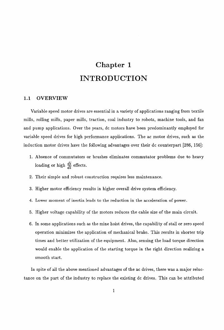
1.1 OVERVIEW

Variable speed motor drives are essential in a variety of applications ranging from textile

mills, rolling mills, paper mills, traction, coal industry to robots, machine tools, and fan

and pump applications. Over the years, dc motors have been predominantly employed for

variable speed drives for high performance applications. The ac motor drives, such as the

induction motor drives have the following advantages over their dc counterpart [286, 156]:

1. Absence of commutators or brushes eliminates commutator problems due to heavy

loading or high a effects.

2. Their simple and robust construction requires less maintenance.

3. Higher motor efficiency results in higher overall drive system efficiency.

4, Lower moment of inertia leads to the reduction in the acceleration of power.

5. Higher voltage capability of the motors reduces the cable size of the main circuit.

6. In some applications such as the mine hoist drives, the capability of stall or zero speed

operation minimizes the application of mechanical brake. This results in shorter trip

times and better utilization of the equipment. Also, sensing the load torque direction

would enable the application of the starting torque in the right direction realizing a

smooth start.

In spite of all the above mentioned advantages of the ac drives, there was a major reluc-

tance on the part of the industry to replace the existing dc drives. This can be attributed

to the following reasons [167, 166]:

1. The cost of the ac power converter far exceeded that of a phase controlled, line com-

mutated reversible converter for the dc machine.

2. While the mechanical construction of the dc motor is complicated, their control is

simple due to the orthogonal field and armature axis. On the other hand, the ac ma-

chines are multi-variable non-linear structures and the totor or currehte-are iffdcces sible. SUES al

The torque is given as a function of the stator and rotor currents. Since the rotor oe amen reine AR He SEO

currents are not accessible without modifications to the machine structure, the con- curtis wit

trol has to be performed through the stator voltages and currents. Hence a complex

control scheme is required to match the converter fed dc drive. This requires sensing

devices, nonlinear electronic components and other devices which increases the cost

and decreases the reliability of the overall drive system.

The recent advances made in the field of semiconductor technology and microelectronics,

has reduced the impact of these constraints. With the advent of vector control, the control

of tl the induction motor is achieved similar to that of a separately excited de motor by

providing independent channels for torque and flux control, induction machines are fast

replacing the dc drives for these applications in the industry [22, 90].

| This chapter is organized as follows. The next section describes in detail the evolution

of the vector control principle and discusses the various vector control strategies. Several

examples involving the application of vector control technique in different industrial ap-

plications will be cited to demonstrate its growing popularity. A comprehensive literature

survey is performed to get an insight into the development of this technique and also to

identify the areas in which more research has to be performed. This is followed by the scope

of this dissertation in Section 1.3. The various issues to be resolved are identified in this

section and the organization of the dissertation is described in the subsequent section.

1.2 STATE OF THE ART

The complexity of the control associated with the induction machines was alleviated by

the advent of vector control in the early ’70s [25, 90]. The main difference between vector

control and the existing schemes for induction machines, such as the constant volts/hertz or

slip frequency control, is that the frequency, and voltage or current imposed on the motor

are controlled without neglecting the phase relationships [129]. Without appropriate phase

angle control, , vector control degenerates into conventional slip frequency ‘control resulting

in poor dynamic characteristics [353]. Vector control was compared with the slip frequency

control and found to have a faster torque response [122]. Quick torque response is achieved

even if a load is applied and the drive system reaches steady state instantaneously. A

comparative study of vector control with the torque angle control and synchronous control

has been performed and the advantages of vector control highlighted [148]. Vector control

is also known as decoupling control since the stator currents are decoupled into separate

torque and flux producing channels. It is also known as field oriented control due to the

fact that the control is based on the field orientation of stator currents.

1.2.1 Classification

Two vector control strategies were formulated during the late 60s and decoupling of

the stator currents was achieved either by the direct measurement of the flux [24] or by

estimation from the motor model [88]. Both these methods are based on the space phasor

modeling of the induction machines [221]. The measurement technique is also known as

flux detection control [162] or flux feedback control [226, 225] since the flux is measured and

fed back into the control circuit. On the other hand, the estimation technique is known as

flux feedforward control or slip frequency control due to the fact that the slip frequency is

calculated from the model for flux estimation.

The flux feedback control uses Halls sensors or search coils to sense airgap flux. Alter-

nately the rotor flux is estimated based on the stator current vector, voltage vector and/or

rotor speed. The flux feedforward control determines the rotor flux from the stator current

signals and rotor speed. An alternate method uses the terminal voltages and line currents

for determining the stator flux derivatives which are then integrated to obtain the flux. Or

else, the terminal voltage, line currents and rotor speed are used as observer quantities to

determine rotor flux [4].

1.2.2 Direct Vector Control

The direct measurement technique was popular in the earlier stages due to the sensi-

tivity of the estimation techniques to motor parameter variations [23]. This technique also

provided instantaneous and well damped control of torque. The earlier forms of this type

of “control involved the measurement of the airgap flux. Field sensing devices utilizing Hall

effect were installed at two or more places within the airgap of the motor to measure the air-

gap flux [169]. The mechanical and thermal stresses on these semiconductor devices caused

problems in measurement. The rotor slot harmonics are filtered and only the fundamental

components are extracted. A detailed description of the placement of the sensing coils for

airgap flux measurement has been presented in [251]. Amorphous microcore sensors were

also used to detect the magnetic field and to sense the torque and rotor currents [219].

Various schemes have been proposed for the sensing of airgap flux. A method for

flux control independent of stator resistance variation based on the magnetizing current

is presented in [1]. This measurement technique performs satisfactorily up to 1 Hz but

the performance degrades at lower speeds. Another method for the measurement of the

airgap flux used the tapped stator windings of the motor [357, 46]. An airgap flux sensing

method was proposed using search coils and providing an open loop flux estimator using the

predictor corrector algorithm [73]. The major disadvantage of airgap flux oriented control

is that the system becomes unstable above a certain critical load [12].

The problem of instability is overcome by using the rotor flux instead of the airgap

flux. Since the rotor flux is not directly accessible, the measurement techniques are even

more complex [9]. A torque drive vector control using the rotor flux orientation presented

problems with the integrator adjustment for obtaining the field angle using LEM transducers

[16]. Another method which measures the stator and rotor flux using Halls sensors to obtain

the field angle and rotor flux, achieved four quadrant operation for fast torque response [63].

The measurement of the rotor flux is dependent on the leakage inductance. A method

using the measurement of the stator flux has been proposed to overcome this effect [340].

The maximum torque capability of this orientation was found to be equal to that of a

properly tuned flux feedforward vector control system. The limitation of the stator flux is

that for low speed operation, it is difficult to obtain a good performance [80]. This is due

to the fact that the stator resistance has to be known or estimated in order to calculate the

stator flux from the terminal voltages.

The rotor flux measurement technique is the most widely used for the flux feedback

vector control strategy. It can be noted that the major disadvantage of the various flux

measurements using different methods is the deterioration of performance at low speeds,

i.e., 3-5% of the rated speed [113]. Also, the delay time in signal processing affects the

dynamic behavior of the drive system because it results in stator current coupling [11].

This effect can be reduced by employing simplified decoupling circuits for the machine and

Oe

transducers and parameter insensitivity.

the inverter. The main effort in research towards this direction is the elimination of the

1.2.3. Indirect Vector Control

Despite the strong incentives such as the absence of transducers and wide speed range

operation, acceptance of the flux feedforward technique has been slow due to its dependence

on the rotor parameters. With the advent of various parameter adaptation schemes to ee

alleviate this problem, it has gained more attention and is widely used for different industrial

applications. A nonlinear model for the saturated induction machines is also derived to take eminem nee

me ae eee te Gh MOTE EE into account the saturation effects on the parameters [320]. The rotor flux is estimated from

the stator currents and rotor speeds, or from line voltage and current measurements. The

field angle is obtained from the induction motor model in synchronously rotating reference

frames.

The components of the rotor flux are also estimated using the state observer technique

and its dynamic and steady state behavior analyzed [14]. In another method, the flux is

estimated using the state observer technique by having the rotor speed and the dc link

voltage as measured quantities [154, 153]. This method for the current source inverter

generates the commanded currents from which the rotor flux and the electromagnetic torque

are estimated. A dual observer technique is employed which simplifies the speed controller

design [44]. Torque control is achieved by using a predictive observer and employing separate

torque and flux feedback loops [89].

An analytic method was presented to detect the spatial position and magnitude of the

rotor flux based on the machine structure using voltage sensors [103]. Another approach

which calculates the speed from the structure of the motor and the measured stator phase

voltages is presented [105, 106]. This method is independent of electromagnetic parameter

variation but is not valid for low speed operation. The effects of the machine structure on

the torque pulsations were studied and the slot rotor structure is found to be unsuitable for

vector control due to problems at low frequencies [312]. Vector control for special motor

structures such as the twin stator induction motor has been proposed [305]. Airgap flux

control for a double cage motor with a current controlled inverter drive was proposed [50].

This provides deep bar compensation to avoid rotor resistance sensitivity and improve the

transient performance [48]. Current control for a doubly fed induction motor was proposed

in [323]. Vector control has been employed for spindle applications with wide constant

power range using dual winding motor [159]. A larger operation range before employing

field weakening is achieved by winding changeover.

1.2.4 Parameter Sensitivity and Adaptation

The major disadvantage of the indirect vector control scheme is that it is machine pa-

rameter dependent since the model of the motor is used for flux estimation. The machine einai,

parameters are affected by variations in the temperature and the saturation levels of the

machine [140, 189]. Parameter sensitivity of the indirect vector controlled induction motor

results in steady state errors in torque and flux and enhanced losses reducing the output of

eter adaptation schemes is required to offset these effects. Numerous parameter adaptation .

schemes have been proposed earlier. Most of the schemes are themselves dependent on some

machine parameters and hence produce different steady state errors which can be used as a

criterion for evaluation of these schemes. The manner in which a scheme affects the dynamic

behavior in terms of bandwidth and stability can be used to assess the advantages of one

scheme over the other. These schemes are classified depending on the extent of the use of

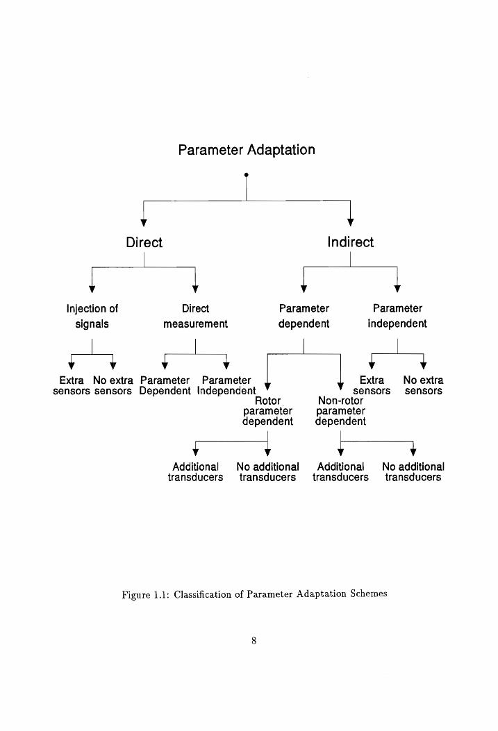
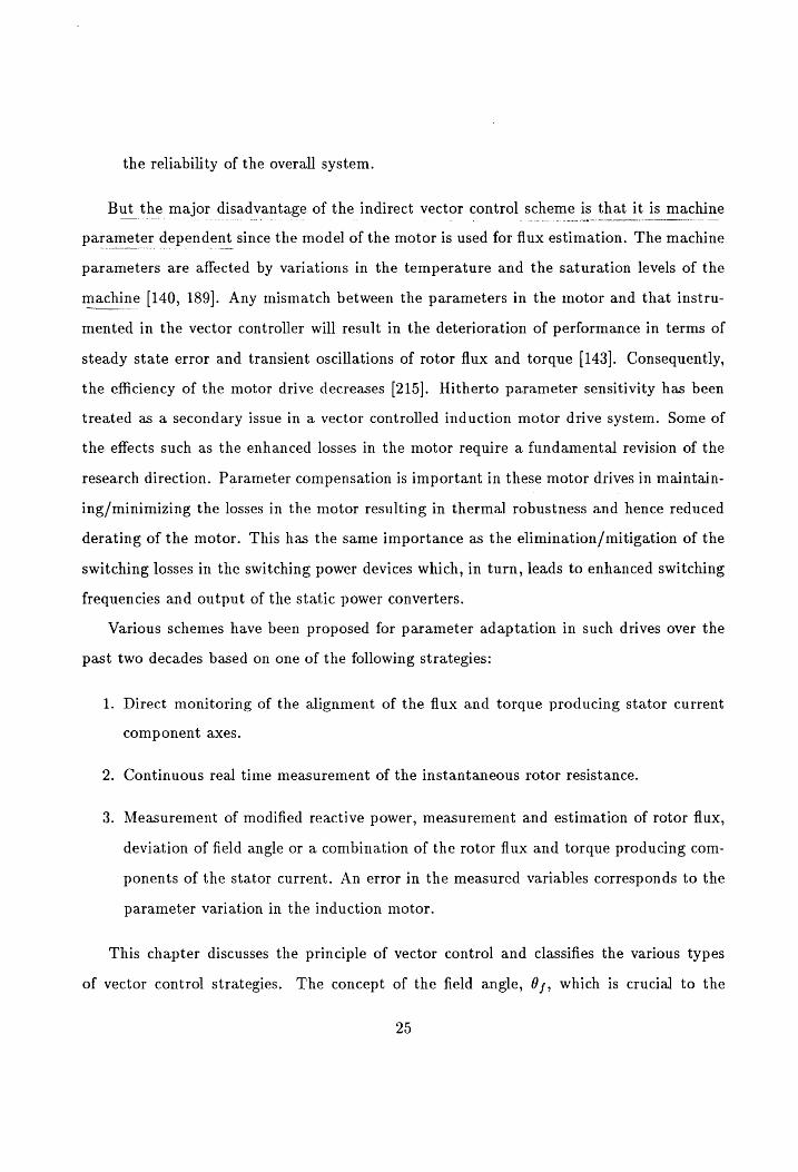
the induction motor model, shown in Fig. 1.1. Parameter adaptation schemes are classified

into direct and indirect methods [135].

Direct Compensation Schemes

The direct method of compensation schemes can be broadly classified into two categories

based on the measurement of the parameters, i.e., either by injecting an external signal

and measuring the parameters or by measuring directly the relevant parameters. They can

further be classified depending on their use of additional transducers or on their dependency

on the motor parameters.

Injection of signals using additional transducers

In the first category, the compensation signal is measured by the injection of some test

signals. Some of these schemes use additional transducers other than the current and speed

sensors required in an indirect vector control scheme [278, 287, 288, 326]. The scheme

proposed in [287] uses the Model Reference Adaptive System (MRAS). A sinusoidal signal

is injected into the flux producing axis of the stator current so that the rotor resistance

is compensated, even when the flux producing current is zero, by satisfying the Popov’s

integral inequality. A similar approach is adopted in [278] and the compensation is provided

by combining a high frequency ac component to the stator current. Both these methods are

influenced by the variation of the stator resistance and require transducers such as search

Parameter Adaptation

|

! |! Direct Indirect

| L

|! |! Injection of Direct Parameter Parameter

signals measurement dependent 1

Extra No extra Parameter Parameter | a Extra No extra sensors sensors Dependent Independent sensors sensors

Rotor Non-rotor parameter parameter dependent dependent

rs ar Additional No additional Additional § No additional

transducers transducers transducers transducers

Figure 1.1: Classification of Parameter Adaptation Schemes

coils. In the scheme proposed in [288] for identification of rotor resistance including zero

speed operation, a high frequency ac component is injected in the field component of the

stator current to produce a high frequency ripple in the rotor flux. By measuring the ac

component of the rotor flux, a change in the rotor resistance is detected which is used

for parameter compensation. A low cost scheme useful in low performance applications

has been proposed to set the controller gain automatically without the need for extensive

testing [326]. In this scheme, the only additional signal required is the feedback signal from

one of the motor line to line voltages. The rotor time constant is measured by injecting

a single phase ac current and the voltage transient that occurs when this test current is

switched to dc is observed.

Injection of signals without additional transducers

The requirement of additional transducers is undesirable as it increases the complexity

and cost of the scheme and reduces its reliability. This disadvantage is eliminated in other

schemes which inject a test signal and sense the corresponding output to provide compensa-

tion (68, 197, 198, 264]. One of the earliest methods used a level characteristic signal, similar

to the white noise having an impulse shaped correlation function, and correlated with the

output to check for error [68]. But the disadvantage of this scheme is that it is difficult to

identify the rotor resistance when the induction motor has zero steady state torque. Also the

injected signal may cause undesirable interference with the performance of the drive. Direct

monitoring of the alignment of the flux and torque producing stator current component axes

is also performed by injecting a negative sequence current perturbation signal (197, 198]. In

this scheme, the voltage corresponding to the negative sequence is sensed and resolved into

d and q axes components. Here the parameters are determined on-line. Another scheme

superimposes a test signal on the voltage reference and the compensation is provided by

monitoring the instantaneous electromagnetic energy and this scheme is independent of the

stator resistance [264].

Direct Measurement and parameter dependent

In the other class of schemes of the direct method, the compensation signal is generated

by the direct monitoring and measurement of motor parameters and alignment of the flux

and torque axis [119, 167, 349]. The scheme proposed in [349] employs additional trans-

ducers and the compensation signal is generated by the direct measurement of the induced

voltage. The compensation signal is dependent on the rotor inductance and this reduces

the reliability of the scheme. The compensation signal can also be generated by using either

the magnitude or the phase of the induced voltages. In the scheme proposed in [167], the

error function is generated by using the vector product of the measured and the calculated

values of the induced voltages. A modified method proposed in [119] uses only the phase

of the measured and calculated values of the induced voltages. Both these methods are

parameter dependent and require additional transducers for compensation.

Direct Measurement and parameter independent

The major disadvantage of the schemes in the previous section is their dependency on

the machine parameters which reduces their reliability. A simple method was proposed for

rotor flux control valid both in steady state and transient operation based on the indirect

measurement through the rotor and stator currents [191]. The rotor currents are directly

measured using two Hall’s transducers placed in quadrature on the shields in front of the ro-

tor ring. The stator reference currents are derived from these measurements which maintain

the rotor flux constant.

Indirect Compensation Schemes

Due to the difficulty in directly measuring all the parameters, the indirect methods have

gained more attention in practical applications. In the indirect method a variable other than

L,, R, and L,, can be measured and tracked and the error due to the difference with its

commanded value provides an estimate of the deviation of the parameter from its nominal

value. For example, the variables may be reactive power, modified reactive power, airgap

power, temperature, etc.

Parameter Dependent

Most of these schemes are dependent on the machine parameters. The variations in

10

these parameters affect the accuracy of the parameter adaptation method itself. Various

schemes have been proposed based on the Model Reference Adaptive Control (MRAC)

technique and most of them fall in this category. In these schemes, the motor adapts to the

changes in the motor parameters after the initial identification. The adaptation functions

by creating an error signal between the motor model reference and an estimated quantity

based on motor outputs. This error will modify the gain in the system until the error is

driven to zero. A tuning algorithm based on this principle was proposed using the torque

model of the controller [184].

Rotor Parameter Dependent using additional transducers

Some of the compensation schemes are dependent on the rotor parameters. A subset

of these schemes use additional transducers [72, 95, 103, 131]. One of the earliest schemes

proposed for rotor time constant compensation is not affected by the stator resistance but

dependent on the leakage inductances [72]. The compensation is provided by defining a

function, modified reactive power in this case, which is computed using the stator currents

and voltages. A variation of this scheme which does not require any more additional trans-

ducers and some integration of key signals was proposed later [131]. The scheme proposed

in [95] is based on the evaluation of the stator current trajectory from a dynamic response

of the induction motor to the PWM switching sequence and this requires additional voltage

transducers. An analytic method was presented to detect the spatial position and magni-

tude of the rotor flux based on the machine structure using voltage sensors [103]. In this

scheme, the parameters are identified by observing the stator voltage corresponding to a

stator ramp current.

Rotor Parameter Dependent without additional transducers

Several schemes which eliminated the requirement of additional transducers were also

proposed [6, 231, 236, 237, 283, 313, 314, 351]. A scheme was proposed for the estimation

of parameters applicable to both steady state and transient operation [6]. In this scheme,

parameter compensation is accomplished by a set of correction factors obtained from the

sensitivity analyses of the performance characteristics. The correction factors are generated

11

using the partial derivatives of the variables with respect to the parameters. In the scheme

proposed in [283], the compensation signal is generated from the error in the estimation of

the flux and the rotor current component without any additional transducers. This scheme

is dependent on the mutual and the rotor inductances. A scheme using the Kalman filter

with the white noise component contained in the three phase PWM switching sequence

was proposed [351]. In this scheme, the result is computed in less than a minute, given an

accurate value of the magnetizing inductance. The limitation of this scheme is that the load

conditions should change gradually and is valid only beyond 0.05 p.u. speed for the effective

functioning of this compensation scheme. Another method based on the discrete MRAC

for identification and compensation of the rotor resistance was proposed [313, 314]. Instead

of the direct compensation for the rotor resistance the slip frequency can also be adjusted.

One such scheme is implemented in a microprocessor by simulating the constant parameter

motor in parallel with the actual motor [231]. Another scheme in which the flux is sensed

from the motor terminal voltages and currents, without Hall sensors or sensing coils was

also proposed in [236, 237]. But this scheme is also dependent on the rotor parameter.

Non-Rotor Parameter Dependent using additional transducers

The major disadvantage of the schemes discussed in the previous section is that the

error function controlling the compensation itself is dependent on the motor parameters

directly affected by the temperature and saturation. A novel scheme has been proposed

which eliminates this problem and is dependent only on the stator resistance [41, 42]. This

scheme uses airgap power equivalence for compensation and does not need any additional

transducers for sensing parameter variation. This scheme is one of the simplest to implement

and has the speed of response required for many high performance industrial applications.

Another scheme dependent only on the stator resistance requiring voltage transducers is

based on the terminal voltages, currents and shaft speed [290]. In this scheme, the rotor

resistance is estimated using tables for mutual inductance and measured terminal quantities.

Non-Rotor Parameter Dependent without additional transducers

Several schemes were proposed which were dependent on non-rotor parameters and

12

require no additional transducers [7, 104, 222, 224, 256]. The schemes proposed in [7] and

[104] are based on the instantaneous input power and electromagnetic torque, respectively.

These schemes are derived from a knowledge of the stator inductance and are valid only in

steady state operation. A simple scheme using the dc link power measurement to estimate

the steady state torque and its use in the analytic calculation of the rotor time constant was

proposed [224]. This is more applicable to steady state than under dynamic operation. A

correlation method using system information from the stator current trajectory to derive the

error angle between the actual flux axis and that of the model using differential equations

and dependent on the stator resistance was proposed [222]. Another MRAC scheme which is

dependent on the stator inductance and stator resistance requiring no additional transducers

was also proposed [256].

Parameter Independent with additional transducers

Some schemes which are independent of the machine parameters were also proposed and

some of them require additional transducers [60, 201, 235, 321, 322]. The scheme proposed

in [235] is based on the slip frequency control with the torque producing current which

is calculated from the stator voltages and currents. The magnitude of the rotor flux is

derived from the magnetic energy independent of the stator resistance and without any

flux transducers. Another algorithm using the hierarchical recursive algorithm to estimate

the stator speed and parameters by measuring the stator currents and voltages has been

presented (201, 321, 322]. In this scheme, the nonlinear model is transformed into a linear

regression model and the variation of parameter is tracked to provide compensation. This

scheme has been verified by simulation but is yet to be implemented. The motor parameters

are also identified by exciting a normal model and the trajectory sensitive model with the

torque component of the stator current and measuring the actual torque [60].

There are numerous variations of the conventional vector control scheme depending on

the application involved. These techniques will be discussed in the following paragraphs.

13

1.2.5 Variations of Vector Control

A variation in the conventional indirect vector control schemes employs the rotor refer-

ence frame model for estimating the rotor flux [276, 275]. This facilitates easier monitoring

of the rotor speed and the motor transfer function exhibits minimum variation with the

rotor speed. This technique has been used for torque control of high performance applica-

tions such as mine hoist drives. The main disadvantage of this system is the sensitivity to

the rotor time constant.

The field acceleration method has been proposed as an alternative for vector control

[347]. It is identical to vector control in basic principle and provides fast torque control [117].

It is based on the equivalent circuit modeling and was attempted for traction applications

[343]. The magnetic field in the airgap is kept at constant amplitude and the speed is

controlled to produce a desired value of torque. By accelerating or decelerating the rotation

of the airgap flux, fast torque control is achieved. A comparative study showed equivalent

transient response for vector control and field acceleration methods [91].

A cycloconverter fed simulator following vector control for a wide speed range has been

proposed for rolling mills [88, 100]. The comparison of current is performed in the d-q

reference frame instead of the three phase reference to eliminate phase delay. This system

is characterized by high speed accuracy, quick response, high power factor and a wide range

of field weakening operation. A Model Reference Adaptive System was also presented for

extending the operation in the field weakening mode [123]. Another variation of the vector

control theory was proposed to achieve quick torque response by controlling the motor

and the inverter together as a single unit resulting in reduced parameter sensitivity [295].

Space vector modulation is employed in this technique to achieve quick response using

current and voltage sensors [294]. The flux is maintained at prescribed levels by using

hysteresis control. This results in reduced torque ripple, low harmonic loss and low noise

[293]. A similar method was proposed for direct stator flux and electromagnetic torque

control [355]. Based on the theory of space vector modulation, a torque angle control for

14

TT mn a

a

a current source inverter fed induction motor drive is also studied [20]. The relationship

between the developed torque, rotor flux and torque angle is analyzed and the torque control

drive is implemented based on this principle [21]. A method for high performance control of

rotor flux which is parameter insensitive is proposed using double hysteresis loop to control

the flux and stator current [245].

A universal theory of indirect vector control for all ac machines based on the modeling

of the salient pole synchronous machines is presented [226]. Scalar decoupled control is

another approach which is very similar to indirect vector control in steady state operation

[31]. It is obtained by a feedforward transfer function for both voltage and current controlled

drives. A synchronous watt torque feed back control is another variation of vector control

which provides better torque control [85]. This involves an additional synchronous torque

loop.

Another approach proposed for control of induction motors is the sliding mode control

which has a good dynamic response, disturbance rejection, low parameter sensitivity [259].

A digital implementation was achieved for which only the bounds of the parameters have

to be known [30]. The main disadvantage of this control is the mathematical complexity of

this approach which is an impediment for practical realization. Direct self control measures

the stator current and flux linkage to control the electromagnetic torque for the entire speed

range including field weakening [55]. Speed regulation is achieved using no speed sensors

using this control strategy [8].

Vector controlled induction motor drive systems are normally voltage source or current

source inverter fed drive systems. A quantitative analysis of the current source and volt-

age source inverter fed induction motor drive has been presented [147]. The small signal

transfer function evaluation has been evaluated for both the strategies using the state vari-

able approach given in [175]. The current source inverter reduces the harmonics, torque

ripple and increases the overall efficiency of the drive system [262]. But it presents torque

fluctuation, low speed response and power factor [238]. Decoupling control with controlled pee chase eH

voltage source exhibits quick rotor response and less sensitivity to rotor resistance variation = a = ~ Smet

15

[232]. A voltage source inverter to generate current commands with improved power factor

is presented in [130]. : The PWM technique is widely employed for inverter fed induction motor drives to

obtain a fast torque response and flux control [18, 81]. Sinusoidal PWM is commonly

applied to analog drives and step PWM is utilized for the digital application. A digital

PWM technique using boxes theory was implemented in [280]. Vector control employing

trapezoidal PWM technique was attempted for a current source inverter to obtain smooth

characteristics [97]. The impact of these strategies on the inverter is presented in [17,

173| and the elimination of harmonics is analyzed in [34]. The current source induction

motor under vector control is modeled and the impact of the dead time in the inverter is

analyzed [306]. An analysis using a voltage fed PWM control where decoupling is achieved

by canceling cross terms between rotor flux and rotor current is performed [298]. A rotor

flux linkage control of a current source inverter fed induction motor drive is presented

with a linear model [302]. The transient performance with regard to computation time

and the PI controller constants is analyzed using this method. A feasibility study of the

transistorized PWM inverter for traction applications has been performed highlighting its

cost and maintenance advantages [247]. An effort to minimize the overall system losses in

this PWM inverter was also attempted [246]. Another optimal study using multi-variable

control for efficiency optimization in a speed controlled system is presented in [211]. In this

method, the ratio of the torque current to the field current is controlled to minimize the

power input.

A speed sensorless scheme was proposed for the constant flux region based on the mea-

surements of voltage and currents [121]. A method which estimates the speed from the

instantaneous slip frequency computation is presented in (220]. The slip frequency is esti-

mated by a filter with no time lag from the voltage and current measurements [218]. This

scheme is very sensitive to the tuning of the proportional and integral gain constants of

the controller. A Model Reference Adaptive System (MRAS) based scheme for rotor speed

identifier capable of four quadrant operation is given in [296]. Another scheme using MRAS

16

using the model of the induction motor in the rotor reference frame estimated the speed

from voltage and current measurements [274]. A sensorless scheme using the voltage and

current measurements insensitive to stator/rotor resistance variation is presented in [234].

The flux estimator included in this method enables control of the system at standstill.

Another scheme achieved speed control without speed sensors and voltage sensors [240].

The change in load torque influences stability and results in flux deviation in this method.

Hence a flux compensation circuit is required for good performance characteristics in four

quadrant operation.

1.2.6 Implementations

Software packages are essential tools for the analysis of the subsystem interaction. Some

efforts were reported for the software package development to analyze the 6 pulse and 12

pulse drive systems [78]. Another study was performed for a flexible multi-axis digital servo

[230]. A PC based vector controller which is applicable for dc, induction and synchronous

machines is presented in this method.

Vector controlled induction motor drives are implemented either by analog or digital

methods. The main advantages of the digital implementation of the vector controller is the

elimination of the offset errors and temperature drift. This results in improved controlla-

bility and reliability [204]. Also, software control is easier and the reduction of components

increases the reliability and the system is extremely noise tolerant [258]. The various meth-

ods available in the literature for the digital implementation of vector control and their

implications would be discussed in the following paragraphs.

A discrete time model of the vector controller is presented using successive time equa-

tions [2]. The system stability of a digital system is discussed from the viewpoints of

sampling period, computation time of the microprocessor and feedback parameters by ex-

amining the loci of the dominant eigenvalues of the state transition matrix and the transient

responses [307]. It concludes that the system has unstable oscillations with high frequency

as the feedback gain or the sampling period is increased even if the dead time is zero, for

17

digital implementations.

The earliest digital implementations employed several eight bit microprocessors to achieve

direct vector control (70, 69]. In this method the flux signals are obtained from the sensing

coils or with stator voltages and currents and four quadrant operation is demonstrated.

Another method employed current tables and different sampling intervals for sensing rotor

speed [209]. The dc link voltage is regulated in this scheme to reduce the current and torque

ripple. A method using look up tables is presented in [36] and another implementation for

constant flux region is given in [342]. A methodology for a single chip microcontroller imple-

mentation was presented in [138]. The main advantage of this system is the reduction in the

chip count which results in increased reliability of control. A current control scheme based

on the space vector modulation technique to achieve quick torque response was implemented

using Digital Signal Processors [200].

A multi microprocessor implementation for the voltage and current source model of

the vector controller is implemented in [87]. A digitalized speed regulator using multi

microprocessors is implemented for the voltage source implementation [149] and another

implementation was proposed for high speed response for the speed drive [213]. Multi

microprocessor based implementation for robust control of the induction motor has been

attempted [311]. In this implementation, vector control is employed for the torque control

and model reference complementary control is used for the speed and position loops. This

control technique guarantees asymptotic tracking/regulation independent of disturbances

and arbitrary perturbations in the drive system parameters. A multi microprocessor based

rolling mill is implemented by employing dc and ac current loops to compensate the funda-

mental output voltage and reduce imbalances of the ac output voltage [263]. The various

practical industrial applications of vector controlled induction motor drive systems will be

discussed in the following paragraphs.

18

1.2.7 Applications

The applications of vector controlled systems in various areas such as pinch roll drives,

traction drives, robots, etc is reviewed in [159]. A current source inverter fed drive is pro-

posed for starting operation for railway traction [54]. For traction drives, the in-rush current

for the induction motor has to be controlled during starting and a method is proposed to

achieve this requirement in [38]. An electric car drive is realized using high reliability control

of a PWM inverter [116].

Vector control has been extensively employed in steel processing plants and the torque

ripple is reduced using PWM techniques [162]. This results in a high quality of steel with

few chatter marks. Another extensive application is in rolling mills such as the seamless

tube piercing mill where precise speed control over wide voltage range is achieved with rapid

acceleration and deceleration characteristics [286]. Vector control also finds applications in

the paper and pulp industry to provide a draw control accuracy of more than 0.2% and

achieves rated torque production at zero speed range [297, 59]. It is also used for paper

machine retrofit applications [252].

Vector control has also been employed in mine hoist drives to provide rapid torque

change and precise speed control over a wide speed range [156]. Various applications in the

process industry have employed vector control strategy [332, 331]. Another application is

for plate mill drives where the cycloconverter fed induction motor drive employing vector

control provides superior performance characteristics compared to the other drive systems

[107]. The most common application is in the servo industry where the vector controlled

induction motor drive is very cost competitive and matches the dc motor performance

[174]. Vector control is fast finding a wide range of application in the textile industry [190].

A vector controlled position drive has been successfully employed for a glue dispensing

equipment to produce a continuous flow of glue around the periphery of a surface [58].

19

1.33 SCOPE

The discussion in the previous section provides an insight into the development of the

different techniques of vector control and their advantages and limitations for various appli-

cations. Based on this survey the following are identified as the key issues to be addressed

in this dissertation:

1. The main obstacle for understanding vector control was the familiarity of the inventor

with space vector modeling [148]. The advantage of this modeling technique is that

the induction motor is treated as two sets of coupled coils resulting in two differen-

tial equations. The d-q modeling approach is the most popular approach in North

America and even though such modeling is available for the indirect vector control

technique in the literature, a comprehensive d-q modeling, simulation and analysis for

the different vector control strategies is yet to be presented. The indirect vector con-

trol scheme, which has gained more attention and acceptance has the disadvantage of

parameter sensitivity. Various adaptation techniques have been proposed to alleviate

this problem. The parameter sensitivity study and the comprehensive study of the

merits and demerits of the different schemes for practical applications is of significant

importance for the success of indirect vector control induction motor drive systems.

2. The induction motor drive system consists of different sub-systems such as the motor,

load, inverter and the controller. With the growing complexity in the development

of the ac drive system, there is a need for more than one engineer to interact in a

research or product development effort. This necessitates a user friendly, interactive,

menu-driven CAE package capable of performing the simulation of the overall drive

system including all the sub-system models, while at the same time providing the

feature to modify each sub-system independently. This would help in the assessment

of the torque ripple, losses, efficiency, torque, speed, and position responses and their

bandwidth and evaluate their suitability for a particular application. Such a package

would reduce the production cost and decrease the product development cycle time.

20

3. Most of the industrial applications require variable speed capability which necessitates

a speed controller. The design and study of the different parameters in a speed con-

troller would help improve the overall performance of the drive system. The similarity

of the vector controlled induction motor drive systems and the separately excited dc

motors has been well established in the literature. Using this relationship, a simple

scheme for the design of the speed controller has been formulated and the implications

studied.

4, Most commercial applications require the elimination of the position sensors from the

vector control strategy. This would help in the reduction of the cost of the overall drive

system and at the same time decrease its complexity due to reduced signal processing.

One such popular example is in automotive applications. The other strong factor for

the elimination of a position sensor is for safety reasons [329]. AC drives are currently

being used for traction for large coal handling equipment. Due to the coal dust and

the hazardous environment, the position sensor has to be explosion proof and should

prevent water infiltration. This along with the difficulty in mounting the position

transducer necessitates a simple and novel sensorless control scheme using the vector

control principle.

5. There is a growing trend towards digital implementation of motor drives due to the

recent advances in microprocessor/DSP technology. The implementation of vector

controlled induction motor drive systems using digital signal processors with built in

peripherals is an added advantage since the reliability of the system increases and

the control by software is easier. Also, immunity to noise, ease of diagnostics, and

reduced component count makes digital implementation an attractive candidate for

modern variable speed drive systems. Hence the experimental verification of the vector

control algorithm is performed using a DSP microcontroller which has built in PWM

controller, timers and I/O ports.

21

Organization of the Dissertation

This dissertation is organized as follows. The next chapter presents the principle of

vector control for induction machines and classifies the different types of vector control

strategy. The modeling, simulation and analysis for these techniques are presented with the

results. Experimental results obtained from the digital implementation for one of the vector

control algorithms is also provided to verify the simulation results. Chapter 3 describes the

systematic derivation of the nonlinear models of the various subsystems involved in an

induction motor drive system and the development of a CAE package, VCIM, is presented.

The integration of the different subsystems and the interaction between them is discussed

and the results obtained from the CAE package are presented to highlight its features

and capabilities. Chapter 4 deals with the design and study of the speed controller for a

speed/position controlled induction motor drive system. The similarity between the vector

controlled induction drive and the dc motor counterpart is utilized to develop the large signal

model similar to that of the dc motor. The simulation results are obtained from the CAE

package, VCIM and the experimental verification is performed using the DSP based setup.

A novel sensorless vector control scheme is formulated and the modeling, simulation and

analysis is presented in Chapter 5. The simulation results and the experimental verification

using a DSP based vector control system is presented to validate the algorithm. The

conclusions are given in Chapter 6. The contribution of this dissertation is presented and the

scope for future research in this area identified. The parameters for the drive system under

study is given in Appendix A and the voltage sensing algorithm employed in the sensorless

technique is presented in Appendix B. The list of symbols used in this dissertation is given

in Appendix C.

22

Chapter 2

VECTOR CONTROL OF INDUCTION

MACHINES

2.1 INTRODUCTION

Separately excited dc motors have been employed for high performance speed and servo

applications till recently despite the fact that ac motors are less expensive, robust and have

low inertia rotors. This was due to the inherent ease of control of a dc motor compared

to an ac motor. Vector control transforms the control of an induction motor to that of a

separately excited dc motor by creating independent channels for flux and torque control.

By reducing the complexity of control of an ac motor, vector control schemes for induction

motor drive systems have gained wide acceptance in high performance applications. Crucial

to the success of the vector control scheme is the knowledge of the instantaneous position of

the rotor flux. Assuming that the rotor flux position is known, the stator current phasor is

resolved along and in quadrature to it. The in-phase component is the field current, 77, and

the quadrature component is the torque current, 7,. The resolution of the current requires

the rotor flux position known as field angle, 0s. This field angle can either be measured

or estimated. Using measured field angle in the control scheme is known as direct vector

control [22] and that using estimated field angle goes by the name of indirect vector control

scheme [90].

The decoupling of the torque and field current channels can be accomplished by con-

trolling a set of stator voltage or current vectors. The vector control schemes are classified

based on these different control strategies. The modeling, simulation and analysis of these

different schemes would help understand the principle of decoupling control. The famil-

23

iarity of the inventor with space vector modeling led to the development of most of the

vector control models using that principle [319]. This technique allows an easier physical

understanding of the operation of the system due to the resolution of the induction motor

model into two differential equations. Another approach employed for modeling the motors

is the d-qg model which transforms an n-phase machine into two fictitious axes known as

the direct or d-axis and the quadrature or the q-axis. This technique lends itself to easier

programming on a computer and is the most widely used technique in North America. The

two axis machine requires less numerical computations than the direct three phase machine

simulation under balanced sinusoidal excitation. This is due to the constant voltage and

constant inductance matrix in the synchronously rotating reference frames. This allows a

larger step length in the numerical integration routine of the motor model [93]. The space

vector modeling approach remained as the chief obstacle against the vector control tech-

nique gaining popularity in USA. This was alleviated to an extent by the development of a

d-q model for the indirect vector control strategy which is available in the literature [143].

A comprehensive d-q modeling, simulation and analysis procedure for the various types of

vector control is yet to be presented.

While there has been a tremendous interest on various strategies of vector control, the

indirect vector control scheme is being favored over the other schemes in many applications.

The increasing popularity of the indirect vector control scheme can be attributed to the

following factors:

e Reluctance to install flux-sensing coils or Hall effect transducers in the stator of the

induction motor which are necessary for direct vector control.

e Ease of operation of the induction motor drive at and around zero speed. This is

due to the difficulty in measurement of the field angle at low speeds, while the field

angle estimation method employed by indirect vector control is independent of the

operating speed.

e Minimization of the number of transducers in the feedback loop and hence increasing

24

the reliability of the overall system.

But the major disadvantage of the indirect vector control scheme is that it is machine

parameter dependent since the model of the motor is used for flux estimation. The machine

parameters are affected by variations in the temperature and the saturation levels of the

machine [140, 189]. Any mismatch between the parameters in the motor and that instru-

mented in the vector controller will result in the deterioration of performance in terms of

steady state error and transient oscillations of rotor flux and torque [143]. Consequently,

the efficiency of the motor drive decreases [215]. Hitherto parameter sensitivity has been

treated as a secondary issue in a vector controlled induction motor drive system. Some of

the effects such as the enhanced losses in the motor require a fundamental revision of the

research direction. Parameter compensation is important in these motor drives in maintain-

ing/minimizing the losses in the motor resulting in thermal robustness and hence reduced

derating of the motor. This has the same importance as the elimination/mitigation of the

switching losses in the switching power devices which, in turn, leads to enhanced switching

frequencies and output of the static power converters.

Various schemes have been proposed for parameter adaptation in such drives over the

past two decades based on one of the following strategies:

1. Direct monitoring of the alignment of the flux and torque producing stator current

component axes.

2. Continuous real time measurement of the instantaneous rotor resistance.

3. Measurement of modified reactive power, measurement and estimation of rotor flux,

deviation of field angle or a combination of the rotor flux and torque producing com-

ponents of the stator current. An error in the measured variables corresponds to the

parameter variation in the induction motor.

This chapter discusses the principle of vector control and classifies the various types

of vector control strategies. The concept of the field angle, #s, which is crucial to the

25

success of any vector control scheme is emphasized with the aid of a phasor diagram in the

next section. Section 2.3 describes the modeling, simulation and analysis of the current

and voltage source direct vector control followed by the current and voltage source indirect

vector control in Section 2.4. The simulation results are validated for the current source

indirect vector controller using a DSP based digital implementation of the controller. The

description of the setup and the results obtained are presented in Section 2.5 followed by a

discussion of the various issues pertaining to vector controlled induction machines.

2.2 PRINCIPLE OF VECTOR CONTROL

The torque is controlled in a dc motor by controlling the armature current while main-

taining the field current constant. This is possible due to the fact that the field and armature

currents can be controlled independently, since the armature and field windings are physi-

cally separate. But in an induction motor, both the rotor flux and the torque are controlled

through the stator currents only. Since there are no separate armature or field windings,

the control becomes complex. One of the important parameters for the vector control is

the rotor flux position, also known as the field angle, 6;. The field angle is defined as the

angle between the stator axis and the rotor field axis.

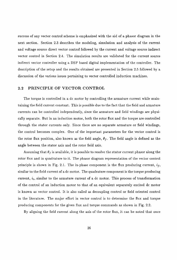
Assuming that 0, is available, it is possible to resolve the stator current phasor along the

rotor flux and in quadrature to it. The phasor diagram representation of the vector control

principle is shown in Fig. 2.1. The in-phase component is the flux producing current, 7,,

similar to the field current of adc motor. The quadrature component is the torque producing

current, 7;, similar to the armature current of a dc motor. This process of transformation

of the control of an induction motor to that of an equivalent separately excited dc motor

is known as vector control. It is also called as decoupling control or field oriented control

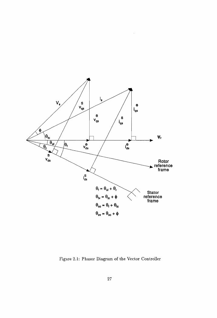
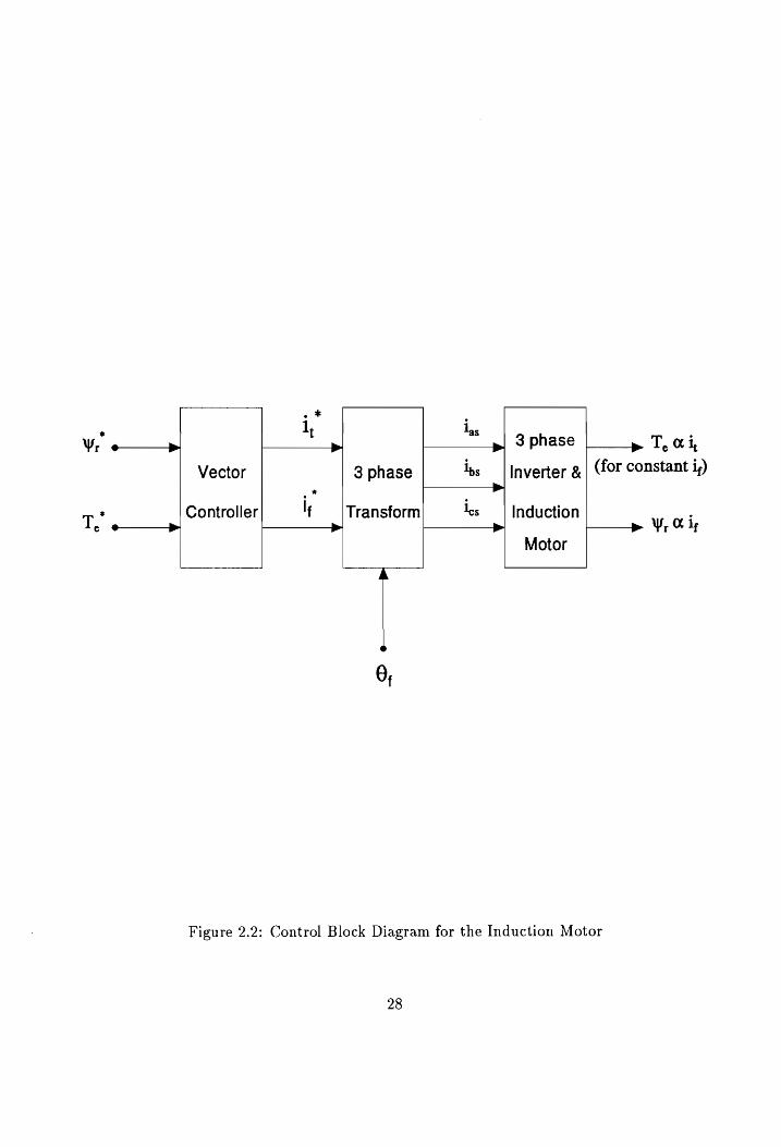
in the literature. The major effort in vector control is to determine the flux and torque

producing components for the given flux and torque commands as shown in Fig. 2.2.

By aligning the field current along the axis of the rotor flux, it can be noted that once

26

Rotor reference frame

Stator Oy =9.+ 0 reference

frame

O., = Oy + Be

By = 8.. + d

Figure 2.1: Phasor Diagram of the Vector Controller

27

Vector

Controller

3 phase

Transform

i,s

Ips

Ics

3 phase

Inverter &

Induction

Motor

| ye T, a i,

(for constant i,)

ye WY, Hig

Figure 2.2: Control Block Diagram for the Induction Motor

28

the value of the rotor flux is obtained, the field angle can be computed. It is also possible

to obtain the field angle by computing the slip angle, 6,;, once the rotor position, 0,, is

known. Based on the method by which the field angle is obtained, vector control schemes

are classified as shown in Fig. 2.3. In the direct method, the field angle is measured from

the outputs of Hall sensors or by integrating the induced emfs from a set of sensing coils

placed near the airgap and embedded in stator slots. The Hall sensors are temperature

sensitive and the sensing coils produce no voltage or very small voltage at standstill and

at very low speeds. This introduces errors and makes the measurement of the field angle

difficult. In the indirect method, the field angle is estimated using the dynamic model of

the induction motor. It can be calculated either through the output of voltage and current

sensors or by measuring the rotor position, 6,, and computing the slip position, 0,;, from

the motor model. The latter method, which needs a position sensor and current sensors, is

the most popular method due to its enhanced reliability.

The dynamic model of the induction motor in the d-q reference frame can be represented

in any arbitrary reference frames. This facilitates the generalization of the model and hence

various models can be derived as particular cases of this model. Three particular cases of

the generalized models of the induction motor in the arbitrary reference frames are most

commonly used. They are:

e Stator reference frame models.

e Rotor reference frame models.

e Synchronously rotating reference frame models.

In the stator reference frame model, the observer is located on the stator of the machine,

while in the rotor reference frame the observer is located on the rotor of the machine. In

the synchronous reference frame, the observer is aligned along the axis of the rotor flux of

the motor. In this reference frame, the d and q axis stator voltages are simplified to dc

quantities and hence their responses will be dc quantities too. From the phasor diagram of

the vector controller, it can be noted that the field current is aligned along the axis of the

29

Vector Control Schemes

| |!

Direct Indirect

(using measured field angle)

'

| | Using computed Using estimated

Current source Voltage source field angle from slip angle and

line voltages and rotor angle to

phase currents get field angle

| |

Current source Voltage source

Figure 2.3: Classification of Vector Control Schemes

30

rotor flux. For ease of analysis, the synchronously rotating reference frames is used for the

dynamic model of the induction motor. Once the field angle is known, the control of the

electromagnetic torque can be enforced by using the stator voltage phasors or the stator

current phasors in the synchronous frame. This leads to the current source and voltage

source of vector control schemes.

2.3 DIRECT VECTOR CONTROL

Direct vector control schemes involve the measurement of the rotor flux, and hence

the field angle, using Hall sensors or sensing coils. The signals that are available for the

control of the induction motor are the field angle and the stator currents obtained from the

current transducers. Normally, only two current transducers are used for a balanced three

phase system and the third phase current is derived as the negative sum of the other two

currents. The torque and flux in the motor can be made to follow their commanded values

by controlling the stator currents through a set of current or voltage vectors. The strategy

which uses the current vectors is known as current source direct vector control and the

technique which uses the voltage vector for the control goes by the name of voltage source

direct vector control.

2.3.1 Current Source

The functional block diagram of the current source direct vector control is shown in

Fig. 2.4. The input to the vector controller is the commanded values of torque and rotor

flux. Using the rotor flux measured by sensors, the commanded value of the stator currents

is generated. The error between the actual and the commanded value of the torque and

rotor flux is processed through a PI controller to obtain the torque and field currents,

respectively. The torque current is directly proportional to the torque in steady state. This

dc value of the torque command is added with the error current to produce the required

level of torque current command. The torque and field currents thus obtained, are then

31

Current

> Offset

Generator

Torque t

Current |

Generator Magnitude _* Angle

i Resolver

W, Field

Current

Generator *

Is

vt Transform- > is

ation | i.

Block *

los

Figure 2.4: Functional Block Diagram of a Current Source Direct Vector Controller

32

processed through a magnitude and angle resolver to obtain the stator current phasor and

the torque angle.

Regardless of the vector control strategy employed, it can be noted that the field current

is oriented along the axis of the rotor flux and the torque current is in quadrature to it. By

inspection from the phasor diagram shown in Fig. 2.1, it can be noted that,

it = ic) (2.1)

is = 1%, (2.2)

The equations for the torque angle and the stator current phasor can be given as,

oe

f

= Vip +i? (2.4)

Since the field angle is available from the Hall sensors, the stator phasor angle for the

* = tan! “ (2.3)

current source vector control can be obtained as,

02. = 0 + 8%, (2.5) Using the two phase to three phase transformation matrix, the commanded values of

the stator currents can be obtained from the following equations:

i*, = iz sin 0%. (2.6)

2 ij, = G sin(;, ~ ) (2.7) eke pe , OT los = 1s sin(95. + 3? (2.8)

These current commands are then processed through a current controller and compared

with the measured values of the actual currents. Using either PWM or hysteresis control

33

techniques the stator currents are controlled to minimize the error and hence produce the

commanded value of torque and flux in the motor.

The model of this vector controller was implemented and the simulation of the overall

drive system performed for this strategy. The output characteristics for a torque drive

employing a current source direct vector control is illustrated in Fig. 2.5. The inputs to

the torque drive are the commanded values of electromagnetic torque and rotor flux. The

rotor speed is maintained at a constant value and the rotor flux is equal to the rated value.

This condition is achieved by starting the simulation with the value of the field current

equal to the rated current. Since the field current is directly proportional to the rotor flux,

this condition ensures that the rotor flux reaches the rated value. The normalized values

of the commanded /actual speed, commanded flux current and the rotor flux, commanded

torque current and the electromagnetic torque, commanded/actual current of phase ‘A’ are

displayed in the figure. It can be noted that the rotor speed is maintained at a constant

value of 0.3 p.u. The inner current loop is represented by the commanded and actual values

of currents. The actual current follows the commanded value, implemented by a PWM

controller at a switching frequency of 1 kHz. A step command of + 0.5 p.u. for the torque

command and a 1 p.u. command for the rotor flux is applied. The actual value of the

electromagnetic torque and rotor flux closely follows the commanded signal. The decoupled

field and torque currents are also given in the figure. The dc value of the torque current

can be noted once the system reaches steady state. The transient and dynamic response of

the current can also be seen in this figure.

2.3.2 Voltage Source

In the voltage source direct vector controller, the torque and flux values are controlled

to follow the commanded torque and flux values by controlling the voltage vectors. The

functional block diagram of the voltage source direct vector control is shown in Fig. 2.6. The

error between the actual and the commanded value of the torque and rotor flux is processed

through a PI controller to obtain the torque and field currents, respectively. From the

34

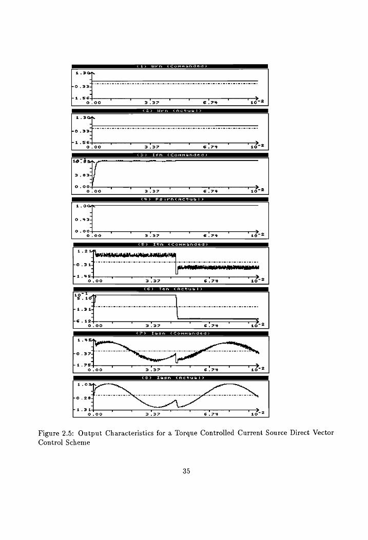
€ 13 Ses ee, ee

Sa ee ee

| os ee

3.83

0.004 7 Cl T T qT t a

0.00 3.37 6.74% 10

Se Fae

1.0

o.43-

0.90 7 t t a 7 T >

6.00 3.37 6.74 1672

ce > ST eee a

(= 2 ek Lek

v OU .

3.3? 6.74% ao72

ha .34-+ 0.00

(S32 Pee ee

», 7.2

3.37 &.7% p He

Figure 2.5: Output Characteristics for a Torque Controlled Current Source Direct Vector

Control Scheme

30

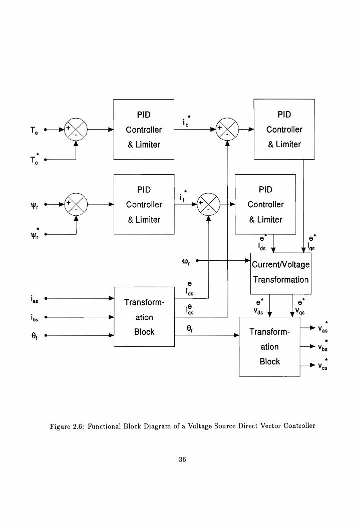
Vr

Vr

36

PID * PID

Controller a Controller

& Limiter & Limiter

PID 4 PID

Controller > Controller

& Limiter & Limiter

| e" las y las

o,° ”/Current/Voltage

e Transformation

|

*| Transform- . e" | | e

> ation as ves was

»! Block 8 Transform- (> ¥

ation

Block

Figure 2.6: Functional Block Diagram of a Voltage Source Direct Vector Controller

measured values of the stator currents the g and d axes stator currents in the synchronously

rotating reference frames is calculated using the following transformation:

tos cos; cos (6 — on) cos (6, + 27) las

is |= 2 sinOf sin (9 — or) sin (@ + “r ) i (2.9) ds 3 f f 3 f 3 bs

in 2 2 3 ics As discussed earlier, the torque and field currents are the g and d axes currents in the

synchronous reference frame for the vector controller. Hence the error between the torque

and g axis current, and the field and d axis current is processed through a PI controller

to obtain the current vectors in the g and d axes, respectively. The transformation from

the current vector to the voltage vector can be achieved using the following equations. The

rotor flux and its derivative are available from the flux sensor and computations. The gq and

d axis rotor currents are given as,

*€ L -€ tor = Tits (2.10)

“e Py Lan -e

‘dr = L, ~ L, tds (2.11)

Hence the commanded values of g and d axes voltages are given as,

* ; . . Lim U5s = Rst55 + LaPtys + We Laids + We I (2.12)

* . . L Vids = Rst4, + Lapras _ WeLatys + FP (2.13)

where,

L?

Ly =1,- = (2.14)

37

The q and d axis voltages can then be transformed to the a, b, and c phase voltage

vectors by using the following transformation,

Vag = Us sin OF, (2.15)

2 of, = v* sin(6%, — =) (2.16)

* * os * 20 Vas = V, sin(Oy, + 3? (2.17)

The three phase voltage vectors thus obtained are then modulated using a PWM con-

troller and the varying duty cycle of the voltage command allows the flux and torque to

follow the commanded values of flux and torque, respectively. With this model of vector

controller, the simulation of the overall drive system is performed for this strategy.

The output characteristics for a speed drive employing a voltage source direct vector

control is illustrated in Fig. 2.7. The input to the speed drive is the commanded value of the

rotor speed. This is compared with the actual value of the rotor speed. The error signal is

amplified and processed through a speed controller to obtain the torque command. The flux

command is obtained from the rotor speed signal with a pre-programmed function generator.

The normalized values of the commanded/actual speed, commanded flux current and the

rotor flux, commanded torque current and the electromagnetic torque, commanded voltage

and actual current of phase ‘A’ are displayed in Fig. 2.7. The inner loop is represented

by the commanded voltage and actual current values. The actual current results from the

commanded values of voltages modulated with a carrier waveform using a PWM controller

at a switching frequency of 1 kHz. A step command of + 0.25 p.u. for the speed command

and a 1 p.u. command of the rotor flux is applied. The electromagnetic torque and rotor

flux closely follow their commanded signal. The decoupled field and torque currents are

also given in the figure. The zero error in the electromagnetic torque indicates steady state

for the drive with no load torque. The transient and dynamic response of the current can

also be seen.

38

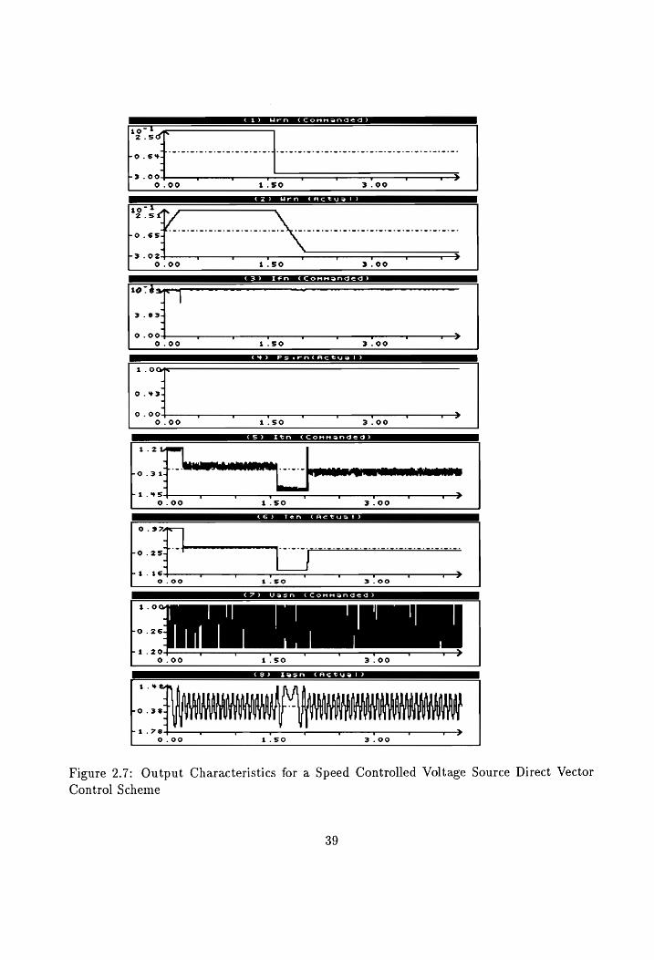
C1). Men CConnanded)

EP Lo. 64d mm mim tw tw emt wwe meet wt wee w ews ee ee ee ee ee ee ee

=

3.00 a 7 7 r > 09.909 1.850 3.990

OS = 0 kn <li OO 190 2.5

Lo est nena ete a eter e reer:

H 3.024 t r r 7 — 0.900 1.890 3.990

On WY 0-0

10°38 —~

3.834

0.00 r T T T T T — 0.00 1.50 3.90

| 4-0

0.434

0.00 . Y > 0.00 1.50 3.00

(CS) Itn CCommanded?)

0.9%.

Lg rrr www we ww we www www ewe:

Pi. 36-4 Tr ¥ ¥ T 7 > 909.9090 %.s90 3.900

Lat en

CCommanded)

¥ 7 Tv ' v v

0.900 1.50 3.00

C8) fFasgn CACKUTID

1.4%

| AAD KU ‘|| ) , i ALOE rFO.38 nal aD a OT PG it Weyl

ri. 78-4 T T T T ——-~ T T T >

9.90 1.50 3.00

Figure 2.7: Output Characteristics for a Speed Controlled Voltage Source Direct Vector

Control Scheme

2.4 INDIRECT VECTOR CONTROL

Unlike the direct vector control technique, the field angle is estimated in the indirect

vector control strategy. The field angle is computed using some measurements and motor

parameters. The slip angle, the commanded values of the stator current phasor, and the

torque angle are estimated using the motor parameters. The rotor position and the stator

phase currents are measured using sensors. From the phasor diagram shown in Fig. 2.1, it

can be noted that the field angle is the sum of the slip angle and the rotor position. Hence

the field angle is estimated using the computed values and control achieved. The torque

and flux in the motor can be made to follow their commanded values by controlling the

stator currents through a set of current or voltage vectors. The strategy which uses the

current vectors is known as current source indirect vector control and the technique which

uses the voltage vector for the control goes by the name of voltage source indirect vector

control.

2.4.1 Current Source

The functional block diagram of the current source indirect vector control is shown in

Fig. 2.8. The indirect vector control algorithm is derived from the dynamic equations of

the induction motor in the synchronously rotating reference frames. The rotor equations in

terms of the rotor flux linkages are,

Ryt5, + PWar + (We _ Wr) Par = 0 (2.18)

RU, + PWar a (We _ Wr) Wor =0 (2.19)

The slip speed is given as,

Ws] = We — Wp (2.20)

As mentioned earlier, the rotor flux phasor is aligned along the d axis. Hence,

40

. L, d 1

YWr° — R, dt Lin

_

x Magnitude . 4 : L, Angle

Tyo N- => Resolver 3P Lin

v N *

. We, > D e Li

N: Numerator

Transform;—> las D: Denominator ation |—> |bs

Block |—~> ;*

Figure 2.8: Functional Block Diagram of a Current Source Indirect Vector Controller

41

Yar = Yr (2.21)

Wqr = 0 = por (2.22)

Substituting equations 2.20 - 2.22 into equations 2.18, 2.19, the rotor equations are given

as,

R, 1%, + Weir = 0 (2.23)

R,t9, + pwr = 0 (2.24)

The rotor flux linkages can be expressed as,

Wor = Lio, + Li’, (2.25)

Pdr = Lig, + Lrig, (2.26)

Hence the rotor currents can be derived as,

tor = F's (2.27)

“e Wr Lm, *e

lar = L, ~ TL, 4 (2.28)

The system equations are then given as,

Lm Ry is sl = - 2.29

CTT L (2-29)

R, e Pb, = TZ. [—v, + Lmitgs] | (2.30)

42

Te = Kyiogr (2.31)

where, A; is the torque constant given as,

3 P Lin _3F 32 M=5aF (2.32)

From these, the commanded values of the torque and flux producing components of the

stator phase currents, 77 and tf, respectively, can be identified and written as,

. et 22 L, TH *_ je* _ Ze 2.33 uy °Os 3 P Lin ar ( )

oo p* 1 L, *

iy =p = 7 [1+ Zp Ploy (2.34)

The equation for the slip speed is then given as,

. _ Iml, sl — R, wr Ww (2.35)

The torque angle and the stator current phasor are obtained using equations 2.3, 2.4.

The stator phasor angle is then given by the following equation:

5c = 651 + Ot + 6, (2.36)

Using the two phase to three phase transformation given in equations 2.6 - 2.8, the

commanded values of the three phase stator currents are obtained. These current commands

are then processed through a current controller and compared with the measured values of

the actual currents. Using either PWM or hysteresis control techniques, the stator currents

are controlled to minimize the error and follow the commanded torque and flux in the motor.

The model of this vector controller was implemented in a PC-based software and the

simulation of the overall drive system performed for this strategy. The output characteristics

for a position drive employing a current source indirect vector control is illustrated in

43

Fig. 2.9. The input is the commanded value of the rotor position. This is compared with

the actual value of the rotor position obtained from the position encoder. The error signal

is amplified and then processed through a position controller to obtain the speed command.

The commanded values of the electromagnetic torque and rotor flux are obtained using a

speed controller and programmed flux function generator. The normalized values of the

commanded/actual speed, commanded /actual torque, commanded/actual current of phase

‘A’ and the command/actual value of rotor position are displayed in Fig. 2.9. The rotor

position command is a ramp signal with a magnitude of + 3 radians. It can be noted that

the actual value of the rotor position closely follows the commanded value. The motor

is at standstill when a constant position command is applied. The torque loop and the

inner current loop control enforce the actual value of the electromagnetic torque and stator

current to follow their commanded values. The inner current loop is implemented by a

PWM current controller at a switching frequency of 1 kHz. and ensures quick response of

the drive system.

2.4.2 Voltage Source

The modeling of the voltage source indirect vector control is very similar to that of

the current source discussed in the earlier subsection. The functional block diagram of the

voltage source indirect vector control is shown in Fig. 2.10. The main difference in this

scheme with the current control scheme is that vector control is achieved by controlling

the voltage phasors rather than the current phasors. The commanded values of the stator

current phasor, torque angle and the field angle are estimated similar to that of the current

source indirect vector control. The g and d axes currents in the synchronous reference

frames are obtained from the measured stator phase currents and the estimated field angle

using the transformation given in equation 2.9. These are compared with the commanded

values of torque and field currents, respectively. The error is then processed through a PI

controller to obtain the g and d axes current vectors in the synchronous reference frame.

The gq and d axis rotor currents, rotor flux and derivative of rotor flux values are calcu-

44

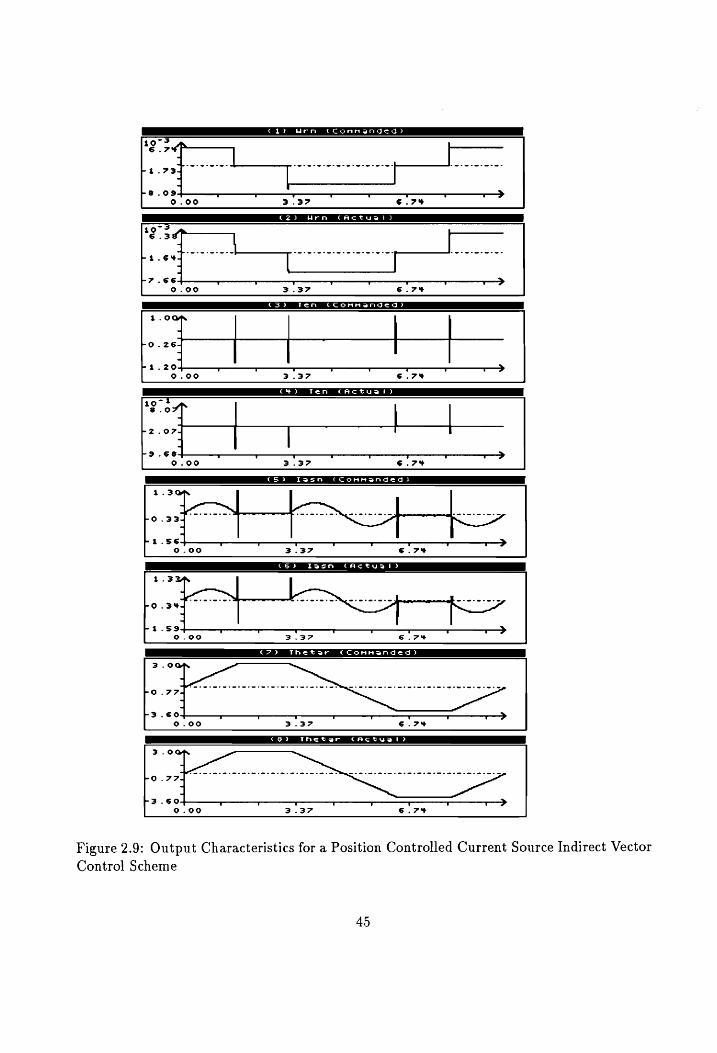
CCONN sanded)

3.37

C2) Mrn CACTUS)

~ 2? 66 Tv t ¥ v v >

0.090 3.37 6.74%

[3s Ten CComnmnanded)

ro .264 | I |

ri. 20 vv Tv v 7 a t v >

0.9090 3.37 6.7%

Cc) Laas CAcCTtusai)

nO ees ee—oro 10

r2z2.074 | { t

rH .68 T T t > 9.9090 3.37 €.7%

cS) Iascn (Commanded?)

1.3

twee miws

T 3.37

>» v gf

T UE

3.37 T

e.7%

>» v F

v

3.37

(ae) tThetar CCommanded)

wv

CS?) tTnetar La Roa eee

9.9090

Figure 2.9: Output Characteristics for a Position Controlled Current Source Indirect Vector

Control Scheme

45

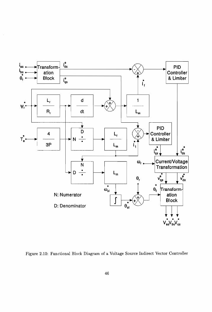
0,» Block [-e

las «—»Transform+_!ds bs ep» ation

qs

. L, d

Wr? R, dt

y

* 4 D

Tyo N - <a

3P

y N

Leip —

N: Numerator

D: Denominator

PID

Controller

& Limiter

{

Lin

PID

Controller

& Limiter

ry eo

lgs lds

Q, »|Current/Voltage Transformation

6, Vas Vas

6, |Transform

ation Block

Ht Vas/ps“cs

Figure 2.10: Functional Block Diagram of a Voltage Source Indirect Vector Controller

46

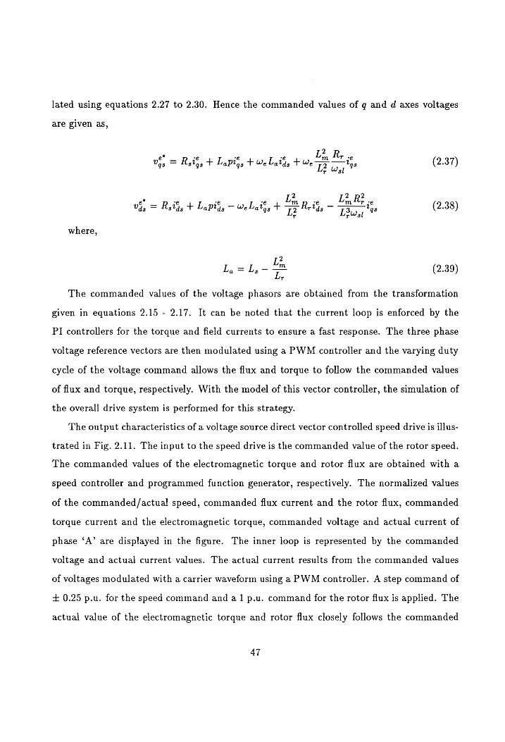
lated using equations 2.27 to 2.30. Hence the commanded values of g and d axes voltages

are given as,

e* _ R *e L “e L *e L?, R, *e 2 37

Ugs = 4tstgs + aPtgs + Webatgs + eT? wy) 98 ( . )

. . . . L? . L? R2. Uf, = Rotis + Lapis ~ velaige + TE Retis — Tos the (2.38)

where,

L?

I, =L,- ZL. (2.39)

The commanded values of the voltage phasors are obtained from the transformation

given in equations 2.15 - 2.17. It can be noted that the current loop is enforced by the

PI controllers for the torque and field currents to ensure a fast response. The three phase

voltage reference vectors are then modulated using a PWM controller and the varying duty

cycle of the voltage command allows the flux and torque to follow the commanded values

of flux and torque, respectively. With the model of this vector controller, the simulation of

the overall drive system is performed for this strategy.

The output characteristics of a voltage source direct vector controlled speed drive is illus-

trated in Fig. 2.11. The input to the speed drive is the commanded value of the rotor speed.

The commanded values of the electromagnetic torque and rotor flux are obtained with a

speed controller and programmed function generator, respectively. The normalized values

of the commanded/actual speed, commanded flux current and the rotor flux, commanded

torque current and the electromagnetic torque, commanded voltage and actual current of

phase ‘A’ are displayed in the figure. The inner loop is represented by the commanded

voltage and actual current values. The actual current results from the commanded values

of voltages modulated with a carrier waveform using a PWM controller. A step command of

+ 0.25 p.u. for the speed command and al p.u. command for the rotor flux is applied. The

actual value of the electromagnetic torque and rotor flux closely follows the commanded

47

©€1)> Herm (CCOMnNanded>

1907 2.s

Lo .6el ewer wr ere ew ee ered wr erwrare: wiwiwrer ere er ere rer esere- ere

- 3.00 T T T T T 7 T v > 0.00 1.S90 3.9090

C2) HWrn CAcTYUa!) |

19

>»

T v v v F

€3) Ifnm (Connandged)

1.890

Lg wg TTT nn ne arn nae ee arene ere re

4 fl

r2.27 ¥ T T T T T T T >

0.00 1.50 3.00

1.0

°o.43-

0.00 r T r > 0.00 1.50 3.00

1.2

Lo gat nn wL-------.---.-- 5-5 eee ee eee:

ri. ¥S+4 FF T ' ¥ v v T v >

0.900 1.50 3.00

(oe) Ten CACctusal>

Lo 26h wpe wee we wie wwe we -w-w. —-~

ri .224 T T T T T T T T > 9.909 i1.s90 3.90

C7?) VUssenm CCommanded)

v

9.900 1.S0 3.99

(3) Tasn CACTVDID

1.8

| AO A | | f Bylipy hi NAD Lie UA bo .39 Ye 1euye ye Pi ay uy WY Puy PY

- 2 81+ v v 1 v a v ' >

9.99 1.50 3.990 Figure 2.11: Output Characteristics for a Speed Controlled Voltage Source Indirect Vector

Control Scheme

48

signal. The similarity with the direct vector control technique can be noted to verify the

validity of the simulation algorithm. The decoupled field and torque currents are also given

in the figure. The zero error in the electromagnetic torque indicates steady state for the

drive with no load torque.

2.5 EXPERIMENTAL VALIDATION

The modeling, simulation and analysis of the different types of vector control were

described in detail in the previous sections and the results presented. It was also seen

that due to the reduced number of transducers and better control performance, the current

source indirect vector control strategy has found wide applications. In this section, a Digital

Signal Processor (DSP) based implementation of such a controller will be described. The

results from this setup will be useful in validating the simulation algorithm and also serve as

a bench mark for implementation of more complicated algorithms such as sensorless vector

control.

The vector controller setup consists of the three different units. They are:

1. Motor and load.

2. Converters.

3. DSP microcontroller.

2.5.1 Motor and Load

A 1HP, 230V, 2 Pole, 60 Hz., 3450 RPM, 3¢ induction motor is used for this study.

The motor parameters and the different constants of the entire drive system are given in

detail in Appendix A. The simulation results in the previous sections were obtained for this

particular drive configuration. The motor is coupled to a dc motor which also acts as a

load. The moment of inertia and the friction coefficient of the induction motor is measured

with the dc motor coupled to the induction motor.

49

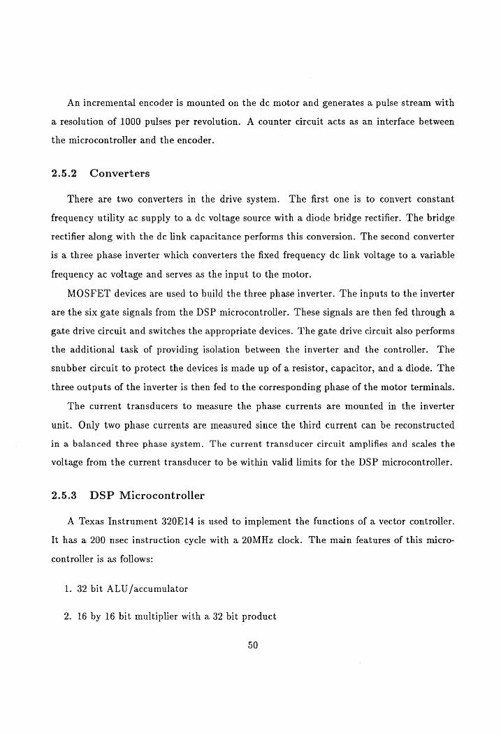
An incremental encoder is mounted on the dc motor and generates a pulse stream with

a resolution of 1000 pulses per revolution. A counter circuit acts as an interface between

the microcontroller and the encoder.

2.5.2 Converters

There are two converters in the drive system. The first one is to convert constant

frequency utility ac supply to a de voltage source with a diode bridge rectifier. The bridge

rectifier along with the dc link capacitance performs this conversion. The second converter

is a three phase inverter which converters the fixed frequency dc link voltage to a variable

frequency ac voltage and serves as the input to the motor.

MOSFET devices are used to build the three phase inverter. The inputs to the inverter

are the six gate signals from the DSP microcontroller. These signals are then fed through a

gate drive circuit and switches the appropriate devices. The gate drive circuit also performs

the additional task of providing isolation between the inverter and the controller. The

snubber circuit to protect the devices is made up of a resistor, capacitor, and a diode. The

three outputs of the inverter is then fed to the corresponding phase of the motor terminals.

The current transducers to measure the phase currents are mounted in the inverter

unit. Only two phase currents are measured since the third current can be reconstructed

in a balanced three phase system. The current transducer circuit amplifies and scales the

voltage from the current transducer to be within valid limits for the DSP microcontroller.

2.5.3. DSP Microcontroller

A Texas Instrument 320E14 is used to implement the functions of a vector controller.

It has a 200 nsec instruction cycle with a 20MHz clock. The main features of this micro-

controller is as follows:

1. 32 bit ALU /accumulator

2. 16 by 16 bit multiplier with a 32 bit product

50

3. 4K word on chip program EPROM

4. Two 16 bit timers

5. Versatile timer event manager with capture and compare outputs

6. Watchdog timer

7. Fifteen external /internal interrupts

8. Seven input and Seven output channels

9. 16 bit bidirectional digital I/O

Power 14, a module designed by Teknic, Inc, has been used for this setup. This module

integrates the DSP microcontroller with the additional peripherals such as the Analog to

Digital Converter, interface with a personal computer, etc. The functions to be performed

by the DSP microcontroller board are as follows:

1. Receive the analog current signals through the ADC and process it for digital calcu-

lations.

2. Receive the encoder pulse output from the counter and calculate the rotor position,

both in clockwise and anti-clockwise directions. The encoder pulse output can either

be received through the capture inputs of the microcontroller or through the digital

I/O ports.

3. Generate the PWM cycle for determining the switching frequency. A 1 kHz switching

frequency is implemented in this controller.

4. Receive the torque/speed commands from an ASCII file and generate the commanded

currents for the three phases using the indirect vector control algorithm.

5. Implement the PWM algorithm by comparing the actual and commanded values of

current.

51

6. Generate the gating signals for the six devices of the inverter using the compare

outputs of the microcontroller.

7. Implement the speed controller which can be a Proportional, Proportional and In-

tegral, or a Proportional and Integral and Derivative controller, for a speed drive

system.

The software for performing the above functions is based on the structure developed

earlier using a single chip microcontroller [138]. The program is modular in structure which

makes the addition of new functions easy. Each task described above are implemented in

the form of subroutines to enhance the modular structure. The PWM cycle generation

is implemented with the aid of the timer interrupts of the processor. The current signals

which are analog in nature, are processed through an analog to digital converter fed into

the processor. The position signal is input to the processor in digital format and only the

incremental position value is computed in the DSP. All the other computations for the

vector control algorithm are performed in the main program using the powerful instruction

set of the DSP/microcontroller.

2.5.4 Results

The simulation and experimental results of the step response of a current source indirect

vector controller is shown in Fig. 2.12. For the speed drive system the actual speed, the

commanded speed and the commanded value of torque is shown in the figure for experi-

mental verification. The commanded value of torque and the actual speed is included from

the simulation results. The step signal is useful to evaluate the dynamic response of the

drive system for the worst case possibility. A step command of + 1000 RPM for the rotor

speed is applied. The speed response closely follows the command value of speed. From

the figure, it can be noted that there is a close correlation between the simulation and the

experimental results.

The simulation and experimental results of the sinusoidal response of a current source

52

1350 5

—1 050 Scale: 100 = 1 p.u.Torque command

—1350

—| 650 LL | ‘ 1 — Le i

0.0 5.2 6.4 9.6 12.8 16.0 Time (sec.)

3 1050 Q 5s

Oo 750 c L

2 450

E 150 & O p

5 -150 oO = Oo Actual speed, RPM (sim.) 2 —450 oO Torque command,p.u. (sim.) N A Speed command, RPM

? Actual speed, RPM (exp.) 2 —/50 Torque command,p.u.(exp.)

Oo

UO © ® Qa

Y

Figure 2.12: Simulation/Experimental Results of Step Speed Response of a Current Source Indirect Vector Controlled Induction Motor Drive

53

indirect vector controller is shown in Fig. 2.13. The actual speed, commanded speed and

the commanded value of torque is shown in the figure for experimental verification and the

simulation results illustrates the behavior of of the drive system. The sinusoidal signal is

useful in determining the bandwidth of the overall drive system. A sinusoidal command

of + 1000 RPM for the rotor speed is applied. The actual value of speed closely follows

the commanded speed and hence the frequency of the commanded signal is within the

bandwidth of the drive system. A close correlation for the experimental and the simulation

results can be observed from the figures.

2.6 DISCUSSION

The various vector control strategies have been classified and the principle of vector

control has been presented in detail. The modeling, simulation and analysis of the cur-

rent /voltage source direct/indirect vector control has been discussed in detail and the re-

sults for the various drive configurations are given to verify the validity of the schemes.

The indirect vector control strategy is gaining more acceptance due to the absence of Halls

sensors and better performance characteristics over a wide speed range. The main disadvan-

tage of the indirect vector control scheme is the dependency on motor parameters. These

parameters change with temperature and saturation which leads to errors in the calculation

of the field angle. Such errors result in poor performance of the motor drives as seen from

the results presented. The parameter sensitivity and compensation study is important from

the point of view of optimum motor and converter use.

To obtain a detailed analysis of the vector control scheme on the induction motors for

any practical application, it is imperative that the entire motor drive system is considered.

The induction motor drive system typically consists of the motor, load, converter and

the controller. Hence it can be noted that in the product development cycle, engineers

involved in various fields have to interact with each other to better understand the overall

drive system for a particular application. This necessitates a Computer Aided Engineering

54

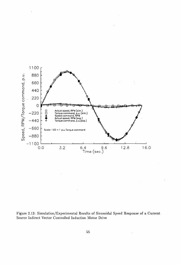
1100

880 |

660

440 |

220

rales dd

ey Arla tbeolmemdinnt Mah AAA a A pamte ad oo co 1 Lar ee

Actual speed, RPM (sim.) Torque command, p.u. (sim.) oO

—220+ OG | A Speed command, RPM

? Actual speed, RPM (exp.) —-440 - Torque command, p.u.(exp.)

Speed, RPM/Torque command, p.

u.

~660 P Scale: 100 = 1 p.u.Torque command

—880 fF

—1100 1 ' , \ ! L i 1 j

0.0 5.2 6.4 9.6 12.8 16.0 Time (sec.)

Figure 2.13: Simulation/Experimental Results of Sinusoidal Speed Response of a Current

Source Indirect Vector Controlled Induction Motor Drive

99

(CAE) package which should be capable of simulating the interaction between the various

subsystems involved in a drive system and provide the input/output in an user friendly

environment. The added advantage of such a package is the resulting standardization of

the terminology which would help in reducing the communication gap. The overall drive

system can also be evaluated by incorporating the different vector control strategies along

with the parameter sensitivity and other modules in such an environment. Such a CAE

package would minimize the product development time and the prototype cost. An effort

has been made in this direction and the development and features of such a CAE package,

VCIM, would be discussed in detail in the next chapter.

56

Chapter 3

CAE ANALYSIS OF THE INDUCTION

MOTOR DRIVE SYSTEM

3.1 INTRODUCTION

With the advent of vector control there has been a growing demand in the industry

for the use of ac machines instead of the dc machines. This, along with the development

in the semiconductor devices and control electronics, has accelerated the growth of vector

controlled ac motor drive systems for variable torque and variable speed applications. The

advantages of the ac drive systems are that they are robust, less expensive, have a higher

power density and require minimum maintenance since there are no brushes or commutators

as in the case of the de drive systems. AC drive systems are multi-input multi-output

systems. A set of stator currents and their frequencies have to be controlled to maintain the

electromagnetic torque and the field flux constant. This increases the order of complexity

of the system and each one of the control variables have a direct influence on the field flux

and electromagnetic torque.

Variable speed drive systems consist of an electric motor, electronic converter, controller

and load. The design of the electronic converter and controller are closely intertwined with

the characteristics of the electric motor and load. The ac machines such as induction, per-

manent magnet synchronous and brushless dc motors, and switched reluctance motors are

nonlinear in nature. Their nonlinearity is further compounded when they are connected to

the power electronic converters which are discrete in nature due to the switching. The inte-

gration of the motor, converter, controller and load to achieve a certain performance index

requires a knowledge of the individual subsystems and their interactions. The development

ov

of new electronically controlled variable speed drive systems is a slow process in the industry

due to a considerable time being spent on their analysis and design. The dynamic simula-

tion is one of the key steps in the validation of the design process of the motor drive system,

eliminating possible mistakes in the prototype construction and testing. While there has

been a considerable amount of research towards the modeling, simulation and analysis of

the drive system, very little attention has been devoted towards the development of a user-

friendly, interactive CAE simulation package. The modeling tools available for these drive

systems are limited since there are no custom-tailored software packages available for this

purpose. Moreover the mathematical models for some of these drives are still evolving in

the research laboratories. With the growing complexity in the development process of an

ac drive system there is a need for more than one engineer to interact in a research or prod-

uct development effort. This enhances the need for a CAE package capable of performing

the simulation of the drive system including the motor, load, inverter, and the controllers

while at the same time providing the feature to modify each subsystem independently. The

ability to simulate the interaction of the subsystems would reduce the production cost and

development time. An effort has been made to fill the need for an interactive simulation

to assess the torque ripple, losses, efficiency, torque, speed and position responses and their

bandwidth and the suitability of the drive system for a particular application.

The models for the vector controlled induction motor drive has been presented in the

earlier chapter. The modeling of permanent magnet synchronous [133, 249] and brushless

dc motor drive [133, 250] and switched reluctance motor drive [133] have been attempted.

A number of factors have not been incorporated earlier. They are:

1. Modeling of the power devices in the converters.

2. Modeling of the various industrial loads in variable speed motor drive dynamics.

3. Modeling of the various speed, torque, and position controllers with limiters.

4. Modeling of the field weakening in the permanent magnet brushless dc and syn-

chronous motor drives.

58

5. Overall efficiency model of the drive systems in steady state.

6. Ripple torque analysis in the variable speed drive systems and Fourier spectrum of

the various currents and voltages in the converters.

7. Frequency response analysis of the entire drive system to obtain the transfer function

and the bode plots.

8. A menu-driven user-friendly steady state and dynamic analysis, design and application

software of these drive systems for use in the research and development environments

both in the industry and academia.

This chapter describes the systematic derivation of the nonlinear models for the vector

controlled induction motor drive systems including their loads and development of a CAE

package, known as VCIM. Based on this principle a set of CAE packages for the brushless

drive systems such as the permanent magnet synchronous, permanent magnet brushless dc

and switched reluctance motor drive systems were also developed. These software packages

are intended for analysis, design and application of these motor drives both in the research

and industrial environment. The chapter is organized as follows. The next section identifies

the requirements of the CAE package for the analysis of any brushless motor drive system.

Section 3.3 describes the induction motor drive system and details the various subsystem

models involved in the entire drive system. This is followed by a description of the CAE

features which are incorporated in the package, VCIM in Section 3.4 and the various issues

relating to its implementation in Section 3.5. The results obtained from VCIM are presented

to highlight the package features in Section 3.6 followed by a discussion on the various issues

relating to the development of CAE packages for such a task.

3.2 CAE SYSTEM REQUIREMENTS

The requirements of a CAE package to perform the dynamic analysis of any brushless

drive system are shown in Fig. 3.1 and include the following: to operate in a PC based

09

CAE for Motor Drive Systems

|

Vector Vector i PM Switched Controlled Controlled Brushless Reluctance Induction PM Sync. DC Motor Motor Motor Motor __

|

File Data Program Output Setup

Handling Manager Execution Results Features

; | Drive | Dynamic i io L File Load Configuration [ Analysis Screen Plot Color

Lo | View oe . nw Default File Schematic Efficiency Print Window

| og: |_ Motor | Frequency Save File Save Parameters Response Setup

L Fj |. Load |_ Fourier File Delete Parameters Analysis

L |_ Inverter | Parameter OS Shell Parameters Sensitivity

| Controller __ Parameter Parameters Adaptation

| Voltage Details

| External References

Figure 3.1: CAE System Requirements

60

environment with file handling, data management, numeric calculation, graphic/tabulated

output and on-line help capabilities.

3.2.1 File Handling

The package should be able to interact with the operating system to enable the user to

save, retrieve and delete files containing the drive system parameters. The ability to work

with several drive system configurations is accomplished by this feature. In an environment

where engineers design subsystems independently, multiple files allow users to vary subsys-

tem parameters without affecting the other drive system modules. In addition, a default file

should be included as a tutorial for new users. Another useful feature in the CAE package

is the ability to exit to the Operating System shell from the program. This would enable

the user to perform DOS operations and return back to package without losing any data in

the computation.

3.2.2 Data Management

A drive system consists of several modules such as motor, inverter, controller, load,

etc. Each subsystem is described by various model dependent parameters. The user of the

CAE package should be able to modify the parameters of each module independently and

at the same time integrate it with the overall drive system. For example, a torque drive

application would not contain the speed controller parameters in the controller module.

3.2.3. Numeric Calculation

For the drive system described by the parameters, the following calculations should be

performed by the CAE package:

1. Dynamic analysis of the drive system.

2. Steady state efficiency characteristics.

61

+

3. Frequency response and transfer function calculations to determine the stability of

the overall drive system.

4, Fourier transform analysis of the current, torque, voltage and speed response of the

drive system.

5. Parameter sensitivity studies.

3.2.4 Output

The simulation of the drive system should produce data that can be examined either

graphically or in tabular form stored in an output file. The user should be able to produce

a hardcopy of the graphic windows. A full screen display containing various output charac-

teristics (in the time or frequency domain) should be provided for the performance analysis

of the entire drive system. A full screen display of each characteristic would allow the user

to study in more detail the drive system behavior. The ability to further zoom into a subset

of the time axis would enable the user to examine the transients.

a

3.2.5 On-line Help

With many software packages, a detailed users manual is required. With improvements

in software design, on-line help should be made available with all software packages. The

following three features would increase the user friendliness of the package and reduce the

importance of the users manual. A brief description of the selected parameter should appear

on the screen as the user edits the various sub-module parameters. At every stage of the

package a help screen should be available to the user upon a single keystroke to provide

information about the selected function and the various options available. An interactive

graphic schema of the drive system would aid the user in understanding the drive system

configuration.

62

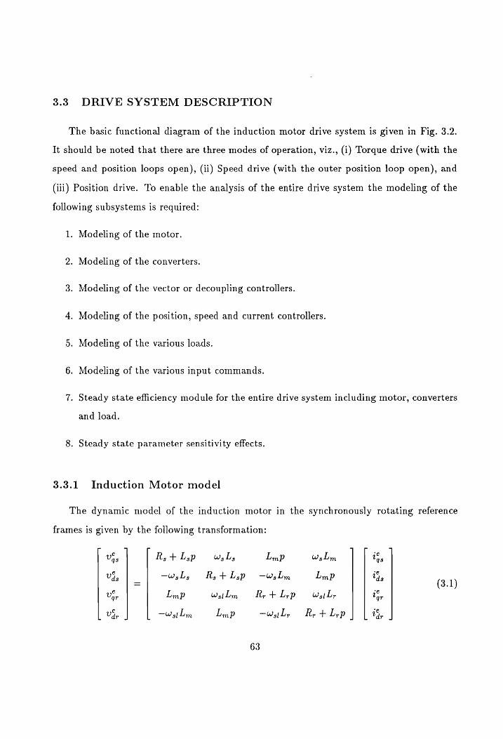
3.3 DRIVE SYSTEM DESCRIPTION

The basic functional diagram of the induction motor drive system is given in Fig. 3.2.

It should be noted that there are three modes of operation, viz., (i) Torque drive (with the

speed and position loops open), (ii) Speed drive (with the outer position loop open), and

(iii) Position drive. To enable the analysis of the entire drive system the modeling of the

following subsystems is required:

1. Modeling of the motor.

2. Modeling of the converters.

3. Modeling of the vector or decoupling controllers.

4. Modeling of the position, speed and current controllers.

5. Modeling of the various loads.

6. Modeling of the various input commands.

7. Steady state efficiency module for the entire drive system including motor, converters

and load.

8. Steady state parameter sensitivity effects.

3.3.1 Induction Motor model

The dynamic model of the induction motor in the synchronously rotating reference

frames is given by the following transformation:

UGs R, + L,p W,sLs LinD Ws Lm ts

Vis —WsLs Rs + Ls —WsLimn Limp Vs ds | _ P d (3.1) Ugr Limp Wsi lm R, + L,p Ws L, tor

V4, —W 5] Lim mp —W.L, R, + L,p Ve

63

ac

main mans y supply .

Rectifier

* Position r Q. Controller

8,

Induction

‘ Filt ‘ Braki wer V, Vi; raking

*

@ Speed

Controller

@,

| Field

Weakening

lac les > +

Inverter Vac

Ty. Tg

Current 4—

Controller

= * *

las lbs Io

*

T, 9 > Vector r

Controller *

W,

Motor

Signal

Processor

Figure 3.2: Vector Controlled Induction Motor Drive System

64

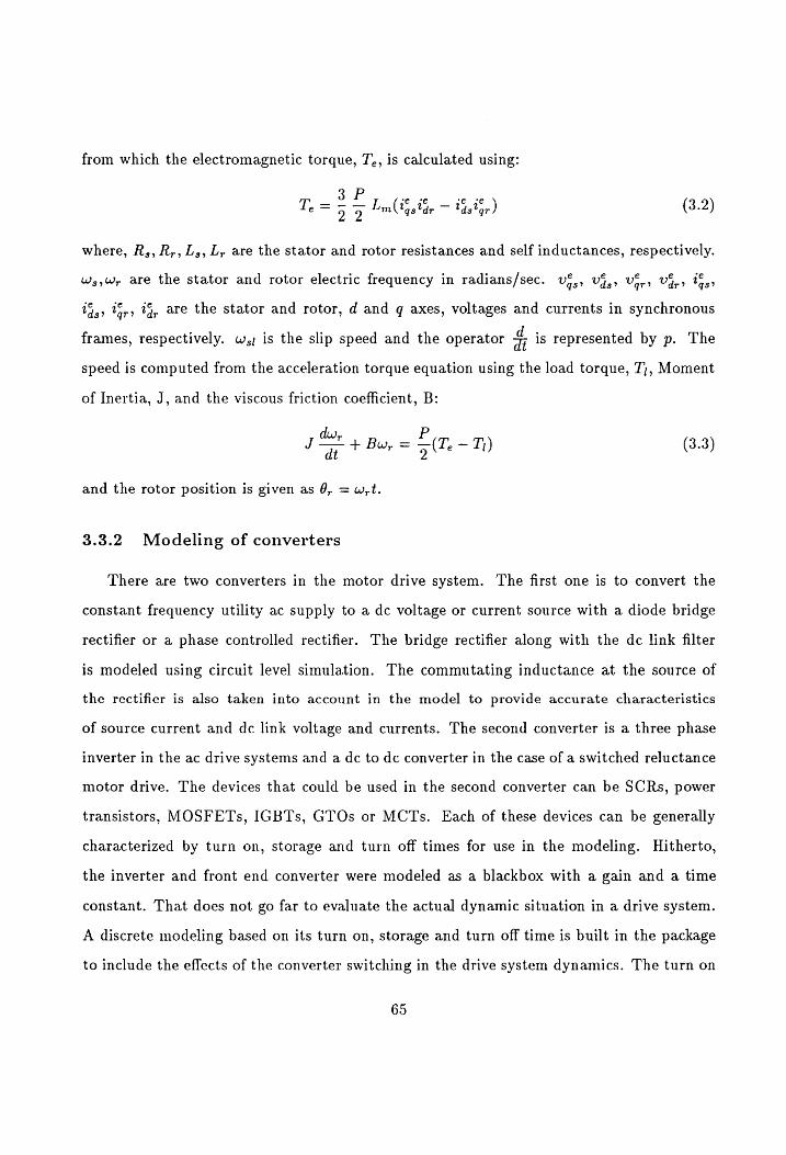
from which the electromagnetic torque, T., is calculated using:

_3P Te —_— 2 2 Lin( iG star ~ tastar) (3.2)

where, R,,R,, L,, L, are the stator and rotor resistances and self inductances, respectively.

W;,W, are the stator and rotor electric frequency in radians/sec. Ugs> Uds> Ugr> Var» tos

tas» Ygr> tgp are the stator and rotor, d and q axes, voltages and currents in synchronous

frames, respectively. w,; is the slip speed and the operator 4. is represented by p. The

speed is computed from the acceleration torque equation using the load torque, 7), Moment

of Inertia, J, and the viscous friction coefficient, B:

dus, ar + Bu, = 5(T.~T1) (3.3)

and the rotor position is given as 0, = w,t.

3.3.2 Modeling of converters

There are two converters in the motor drive system. The first one is to convert the

constant frequency utility ac supply to a dc voltage or current source with a diode bridge

rectifier or a phase controlled rectifier. The bridge rectifier along with the dc link filter

is modeled using circuit level simulation. The commutating inductance at the source of

the rectifier is also taken into account in the model to provide accurate characteristics

of source current and dc link voltage and currents. The second converter is a three phase

inverter in the ac drive systems and a dc to dc converter in the case of a switched reluctance

motor drive. The devices that could be used in the second converter can be SCRs, power

transistors, MOSFETs, IGBTs, GTQs or MCTs. Each of these devices can be generally

characterized by turn on, storage and turn off times for use in the modeling. Hitherto,

the inverter and front end converter were modeled as a blackbox with a gain and a time

constant. That does not go far to evaluate the actual dynamic situation in a drive system.

A discrete modeling based on its turn on, storage and turn off time is built in the package

to include the effects of the converter switching in the drive system dynamics. The turn on

65

and turn off stresses are relieved by the snubber circuits and are modeled as they are in the

simulation to obtain the true switching picture and hence to get the switching stresses on

the devices in the converters. This will enable the sizing of the required converter power

devices and the filters.

3.3.3 Modeling of the vector controllers

AC motor drives such as the induction and permanent magnet synchronous and brushless

motor drive systems are multi-input multi-output systems. To control the electromagnetic

torque and field flux, a set of stator currents and their frequencies have to be controlled.

The number of control variables become too many and each one of these has a direct

influence on the field flux and electromagnetic torque. Independent control of the field

flux and torque is required for high performance applications. That is made possible by a

decoupling controller. This decoupling controller will transform the torque and field flux

commands into equivalent current commands to influence these variables independently.

This is similar to the dc motor drive where field flux is controlled by the field current and

torque by the armature current, if the field current is maintained constant. Hence the

decoupling controller transforms the control of the ac motor into that of an equivalent dc

motor drive. This will enable the independent control of field flux and electromagnetic

torque, thus simplifying the control task of an ac motor drive which is a multi-input multi-

output system. A class of decoupling controllers, known as vector controllers, has been

widely accepted in the industry.

If the rotor field flux is available for feedback control then it is known as direct vector

controller and if the field flux is computed then it is known as indirect vector controller.

Many high performance systems fall under the latter category. The disadvantage of the

indirect vector controller is that it is dependent on the motor parameters such as the mutual

inductance, rotor self inductance and rotor resistance. All these motor parameters are

sensitive to variation in saturation levels and temperature. This will result in the coupling

of the flux and torque channels, contrary to the intended objectives of their decoupling.

66

Hence it becomes necessary to know the effects of the parameter sensitivity on the drive

system performance both in steady state and dynamic situations. A systematic derivation

of the various algorithms is given in Chapter 2.

3.3.4. Modeling of the current, speed and position controllers

Current controllers

The current controllers determine the speed of response of the current loop and hence the

torque generation in the machine. Apart from the speed of response of the current loop, it

is desirable to minimize the current harmonics and hence the torque ripple. Various current

controllers have come into existence with different performance indexes for use in the vector

controlled induction, permanent magnet synchronous and brushless dc motor drives. The

most widely used current controllers are viz., (i) Pulse Width Modulated (PWM) current

controllers, and (ii) Hysteresis current controllers.

It is important to assess the impact of the power device characteristics, motor parame-

ters, and load parameters on the performance of the current controllers and hence the total

drive system, for a given application to identify the most suitable current control strategy

and current controller. These controllers are modeled and integrated in the CAE package

to study the research implications of the various current control strategies.

Speed and Position controllers

The speed and position controllers determine the dynamics of the drive system with

reference to the rise time and overshoot and also offset the mechanical resonances in the

load. It is usual to use a proportional or proportional and integral or a proportional-

integral-derivative controller in the industry. But the tuning of this controller to achieve a

certain performance with the nonlinear motor drive is a time consuming process if trial and

error approach is resorted to. From the frequency response, the controller parameters can

be chosen to closely approximate the control specifications. Then the tuning can be done

67

within a few iterations taking fully into account the nonlinearity of the motor drive system.

3.3.5 Load modeling

Until now in the literature, the load is modeled as an inertia and a frictional constant. It

is unusual to encounter such a simplistic load in practice and this fact calls for the simulation

of realistic loads such as fan, pump, compressor and nonlinear loads driven by the ac drive

systems. The load modeling and the study of its effect on the drive system performance has

manifold advantages of precisely sizing the converter, motor and determining in advance

any of the mechanical resonance and oscillation problems when driven from the ac drive

systems. These oscillation problems if confirmed in the simulation could be overcome by

the judicious selection of the parameters in the speed and current controllers.

3.3.6 Modeling of the reference inputs and disturbances

The reference inputs and disturbances required for application to evaluate the dynamic

drive system performance are identified to be any one of the following:

1. Step signal input.

2. Trapezoidal signal input.

3. Sinusoidal signal input.

The step signal for input or disturbance is chosen with a view to evaluate the dynamic

responses of the drive system in the worst case. The trapezoidal signal is intended for

testing the drive system under realistic industrial conditions. The sinusoids with flexibility

for biasing them positive or negative are intended for finding the bandwidth under all the

nonlinearities and to study the effects of excitation under resonance. A great amount of

programmability and flexibility is built into these test signals so that they can satisfy most

of the realistic needs of the user.

68

3.3.7 Steady state efficiency module

The computation of the steady state efficiency is required to optimize the control strategy

and to reduce the operating energy costs of the drive system. Also this module is intended to

compare the various drive systems and this is one of the authentic criterion for comparison in

many of the appliance drives such as refrigerator, freezer, washer, dryer and hvac compressor

motor drives. Such an efficiency calculation should include not only the motor but also the

inverter and controlled or uncontrolled rectifier used for ac to de power conversion. The

algorithm proposed considers all the losses in the electronic converter switches, diodes, and

motor. The motor losses will include all the copper losses and core losses which are available

either as a constant or a function of operating frequency. The friction and windage losses

are given as a constant for a particular speed or entered as a function of speed through

graphical means. The overall efficiency is evaluated as the ratio of the rotor output to the

input of the electronic converter from the ac mains supply. An instantaneous calculation of

efficiency will be difficult to interpret as there is an interchange of energy from the source to

motor and vice versa. The input and output are averaged over the period of 360 mechanical

degrees and then the efficiency is calculated from these average values.

3.3.8 Steady state parameter sensitivity module

The indirect vector control strategy is dependent on the rotor resistance, R,, the mutual

inductance, L,,, and the self inductance of the rotor, L,. The inductances change with the

saturation of the magnetic material while the rotor resistance is affected by the variation

in the temperature [132]. The increase in temperature increases the rotor resistance. In

case of the current source inverters used in high performance drive systems, if the stator

current is maintained constant this has the effect of increasing the magnetizing current and

hence saturating the machine. Core losses in the motor increases with the saturation of the

magnetic path and in the end necessitates a considerable derating of the machine.

In a torque controlled induction motor drive, i.e., with the outer speed loop open, the

69

rotor flux linkages and the electromagnetic torque are the external command signals while

the actual slip speed is maintained equal to the command value. The mismatch between the

controller and the motor parameters introduces deviations in the flux and torque producing

components of the stator current and hence the torque angle. Once the outer speed loop

is closed, the electromagnetic torque, T7, will be modified until the actual output torque

equals the load torque in steady state. Thus, the effect of parameter variations on steady

state performance is reduced. The temperature and saturation effects are studied for the

torque, flux, slip speed and the peak stator current phasor.

3.3.9 Drive systems

The features discussed in the earlier sections for the vector controlled induction motor

drive systems can also be used in the development of CAE packages for the following

brushless drive systems:

1. Permanent magnet synchronous motor drive system.

2. Permanent magnet brushless dc motor drive system [137].

3. Switched reluctance motor drive system [13, 284].

All the features discussed in the earlier sections are incorporated for all these drive

systems listed above. For the case of a switched reluctance motor drive system, in addition

to the development of the dynamic simulation package, SRMDYN, the task included the

integration of other software packages into a single powerful tool. The author had earlier

been involved in the development of a CAD package for the design and analysis of a switched

reluctance motor and a steady state analysis package of the converter for the switched

reluctance motor [284]. These packages are currently integrated into a single CAE tool,

known as SRMCAD, which combines the features and functions of all the three packages.

These CAE systems constitute the development of modern drive systems for which no such

analysis software packages are currently available. Still quite a number of industrial houses

70

are in the process of developing these advanced drive systems and these CAE packages will

be of help in their efforts.

3.4 CAE SYSTEM FEATURES

The major features required by the CAE package to perform the above task are identified

as follows:

— . File management.

2. Data development.

3. Run commands.

4. Plot commands.

5. Setup choices.

6. Help features.

7. Quit command.

Each of the above features has a set of options and they will be individually described

in the following subsections.

3.4.1 File management

Four options are available for this feature and they are:

1. Default drive system for loading.

2. User-defined system for loading.

3. Save the current drive system.

4. Exit to Operating System.

71

The default drive system is for tutorial purposes to help the beginner. The user-defined

system stores all the drive systems that the user may have worked on and any one of them

can be loaded for future simulations. The save option stores the current drive system that

the user maybe working on into the disk space for future use. The option to exit from the

CAE package to the operating system enables the user to perform some basic operation

outside the CAE shell without losing the current data environment.

3.4.2 Data development

The data development section has the following features:

1. Drive configuration.

2. Schematic of the drive system.

3. Motor parameters.

4. Load parameters.

5. Inverter parameters.

6. Controller parameters.

7. External references.

These features are explained in the following paragraphs.

Drive configuration

This capability facilitates the selection of different types of drive configuration. The

possible choices are the torque, speed or position drive. The torque drive has the speed and

position loop open, while the speed drive has the outer position loop open.

72

Drive schematic

The drive schematic has the capability to provide a graphical representation of the

torque, speed, and position drive systems. A sample output of a position drive schematic is

given in Fig. 3.3. The individual subsystems are displayed in detail upon the user’s request

made possible by moving a lens/cursor on each one of them. The torque, speed, and position

controlled drive schematics are given in this module. This feature would help a new engineer

to become familiar with the entire drive system. Also, if more than one individual is working

on a development effort, the schematic would enable them to communicate with each other

due to the standardization of the symbols and notations.

Motor parameters

The motor parameters such as inductances, resistances, emf constant, power, voltage,

frequency, friction coefficient, and moment of inertia, etc., are defined and included in this

module. A brief definition of the parameter selected is described in the window box placed

at the bottom of the screen with its standard units to help the user.

3.4.3 Inverter parameters

The inverter switches are characterized by the turn on, storage and turn off times,

conduction voltage drop and the voltage drop across the free-wheeling diode which is anti-

parallel to the switch. Apart from these, the snubber resistor and capacitor values are

obtained to model the turn-off process completely.

The input rectifier which converts the ac source to a constant dc link voltage is modeled

either a controlled or an uncontrolled rectifier. The dc link voltage is characterized by:

Vac = 1.35Vi cos a (3.4)

where V; is the line-line voltage and a is the triggering angle. For uncontrolled rectifiers,

the triggering angle is 0 degrees.

73

Current Sorte Indirect Yector Controle | M Postion Drive

Suna etifie ae Filter] at

I Progran ae

he

Fl Detailed blocks Esc cuit We

Figure 3.3: Sample Output of the Position Drive Schematic

74

3.4.4 Controller parameters

The controller parameters consists of the following independent modules:

1. Current controller.

i]

. Speed/position controller.

3. Current limiter.

4. Torque/speed limiter.

5. Field weakening.

A brief explanation of each module listed above is given in the following paragraphs.

Current controller

There are two options for current control, viz., hysteresis and pulse-width modulated

(PWM) current controllers. The hysteresis current controller is characterized by the current

window, i.e., the current deviation allowed for the actual current from the value of the

reference current. The PWM current controller is characterized by the carrier frequency,

and the current controller gain.

The PWM current controller equation is given as follows for phase ‘A’. A similar rela-

tionship holds for ‘B’ and ‘C’ phases.

“§¢ — device drops if tg, — 73, > carrier amp. Vas = (3.5) V. ae

——ge + device drops if tas — 13, < carrier amp.

where ig, and V,, are the phase ‘A’ current and voltage, respectively. Vu- is the dc

link voltage. The hysteresis current controller for one phase, say ‘A’, satisfies the following

conditions:

79

V,, = — Ye + device drops if tg, — 7%, > A; (3.6)

Vie — device drops if tgs —2*. < A; as

Speed/position controllers

Three type of speed/position controllers are implemented for the drive systems and

they are proportional (P) type, proportional integral (PI) type or proportional integral and

derivative (PID) type. These would require the proportional, integral and derivative gains

depending upon which speed/position controller is chosen.

The position controller to calculate the speed command for any position error signal is:

d( 6" ~ 6, )

dt

The speed controller to calculate the torque command for any speed error signal is:

w* = K,(0" — 6,) + Ki | (6 ~6,)dt + Ka (3.7)

d(wr — Wy)

dt

where, A,, AK; and Kg are the proportional, integral and derivative gain constants

Tt = Ky(wt —w,) + Ki / (wt —w,)dt + Ka (3.8)

respectively.

Current limiter

The current limiter is required for the purpose of primarily protecting the converter and

the process from thermal breakdown and catastrophe, respectively. This current limiter

is dependent upon the converter capability, motor ratings and load restrictions. They are

usually in the range of 1 to 6 p.u. in practice. Therefore, a flexible current limiter is built

into this software package.

Torque/speed limiter

The torque/speed limiter serves a similar purpose by limiting the torque/speed command

signal. A variable limiter is built into the software package.

76

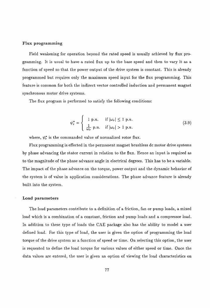
Flux programming

Field weakening for operation beyond the rated speed is usually achieved by flux pro-

gramming. It is usual to have a rated flux up to the base speed and then to vary it as a

function of speed so that the power output of the drive system is constant. This is already

programmed but requires only the maximum speed input for the flux programming. This

feature is common for both the indirect vector controlled induction and permanent magnet

synchronous motor drive systems.

The flux program is performed to satisfy the following conditions:

lp.u. if |w,| < 1 p.u. wv, = 1 . (3.9)

a pu. if |w,| > 1 p.u.

where, ~* is the commanded value of normalized rotor flux.

Flux programming is effected in the permanent magnet brushless dc motor drive systems

by phase advancing the stator current in relation to the flux. Hence an input is required as

to the magnitude of the phase advance angle in electrical degrees. This has to be a variable.

The impact of the phase advance on the torque, power output and the dynamic behavior of

the system is of value in application considerations. The phase advance feature is already

built into the system.

Load parameters

The load parameters contribute to a definition of a friction, fan or pump loads, a mixed

load which is a combination of a constant, friction and pump loads and a compressor load.

In addition to these type of loads the CAE package also has the ability to model a user

defined load. For this type of load, the user is given the option of programming the load

torque of the drive system as a function of speed or time. On selecting this option, the user

is requested to define the load torque for various values of either speed or time. Once the

data values are entered, the user is given an option of viewing the load characteristics on

77

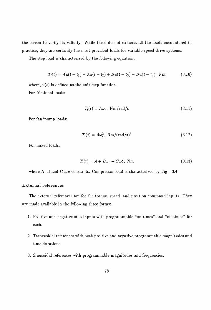
the screen to verify its validity. While these do not exhaust all the loads encountered in

practice, they are certainly the most prevalent loads for variable speed drive systems.

The step load is characterized by the following equation:

Ti(t) = Au(t _ ty) _ Au(t _ te) + Bult _ tz) _ Bult _ ta), Nm (3.10)

where, u(t) is defined as the unit step function.

For frictional loads:

T,(t) = Aw,, Nm/rad/s (3.11)

For fan/pump loads:

T(t) = Aw?, Nm/(rad/s)? (3.12)

For mixed loads:

T(t) = A+ Bu, + Cw?, Nm (3.13)

where A, B and C are constants. Compressor load is characterized by Fig. 3.4.

External references

The external references are for the torque, speed, and position command inputs. They

are made available in the following three forms:

1. Positive and negative step inputs with programmable “on times” and “off times” for

each.

2. Trapezoidal references with both positive and negative programmable magnitudes and

time durations.

3. Sinusoidal references with programmable magnitudes and frequencies.

78

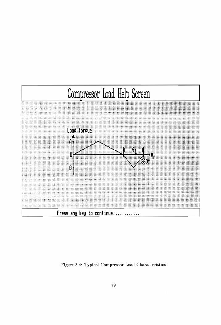
Press any key to continue...

Figure 3.4: Typical Compressor Load Characteristics

79

The step reference is for the purpose of evaluating the time domain performance of

the drive system for torque, speed, and position inputs and disturbances. The trapezoidal

references closely resemble the references encountered in practice and hence will be useful

in evaluating an actual application. The sinusoidal references can be used to evaluate the

bandwidth of the position, speed, or torque loop by observing the attenuation for increasing

input frequencies. It should be noted that this type of evaluation involves no approximations

in the converter or linearization of the motor and controller equations. This is the only way

the speed or current loop bandwidth can be estimated in the motor drive systems. Step

responses are also important to characterize a system such as a fast response robotic drive.

These reference signals have been incorporated into the software packages with the input

parameters defined in Fig. 3.5.

3.4.5 Run options

The requirements of the run option include:

1. Dynamic simulation of the entire drive system.

i)

. Steady state efficiency calculation.

3. Fast Fourier Transform of current, voltage, torque and speed.

4. Parameter Sensitivity study.

A full screen display describing all the drive parameters prior to these run commands

helps to verify the parameters. A hard copy of the screen can also be used for documen-

tation purposes. During execution of the commands, the progress of the calculation is also

reported. These features enhance the usefulness of the software package.

3.4.6 Plot features

The capability to plot on a screen or printer is required for a graphical analysis of the

simulations. Additional features such as the selection of variables for plotting and zooming

80

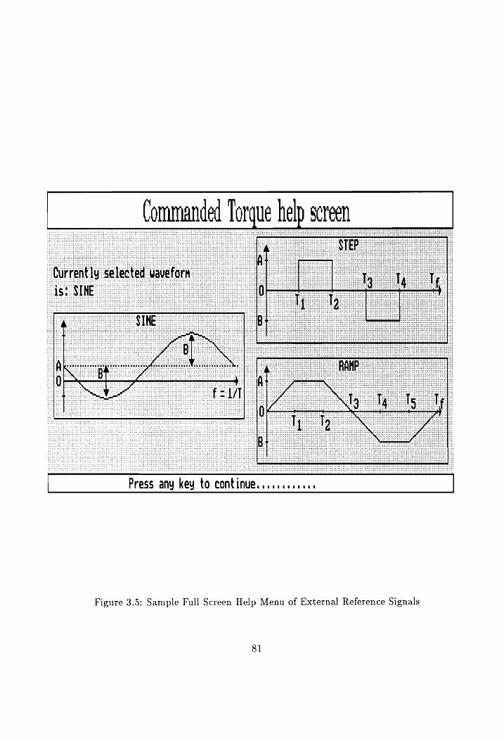
Commanded Torque help screen

“Currently ‘Sele

cist SINE. |

Press any key to continu@.cccsececece

Figure 3.5: Sample Full Screen Help Menu of External Reference Signals

81

to examine in detail the torque and current waveforms for ripples, etc., is incorporated for

enhancing the analysis capability. An added feature is the option to micro zoom into any

plot which helps in the detailed study of the drive system characteristics.

3.4.7 Setup features

The setup of the colors for various levels of the menu screen is required for increasing

the comfort zone of an individual user. Output files should be set for different variables of

interest in the drive system.

3.4.8 Help features and users manual

Context-sensitive help in the form of pull-down screens is required whenever the user

needs it. Interactive help screens available upon a single keystroke eliminates the need for

detailed user manuals. This can be made much more sectionalized and indexed to make

it into a manual for beginners using these CAE packages. These manuals can be either in

script or readme type of files. The CAE packages have been developed for the modern drive

systems satisfying the criteria listed in the previous sections. The main features of the CAE

packages are summarized below:

e The CAE system, developed in PASCAL and FORTRAN, is highly interactive with

powerful graphics capability. A context-sensitive, detailed on-line help is available on

a single keystroke.

e The I/O structure utilizes easy-to-use window-based pull-down menus.

e A default drive system is provided in a file and may be used as a tutorial for the new

users.

e The CAE packages are capable of simulating a torque, speed, and a position drive.

e An on-line schema for a torque, speed or a position drive is available with a built-in

option to magnify any block in the drive.

82

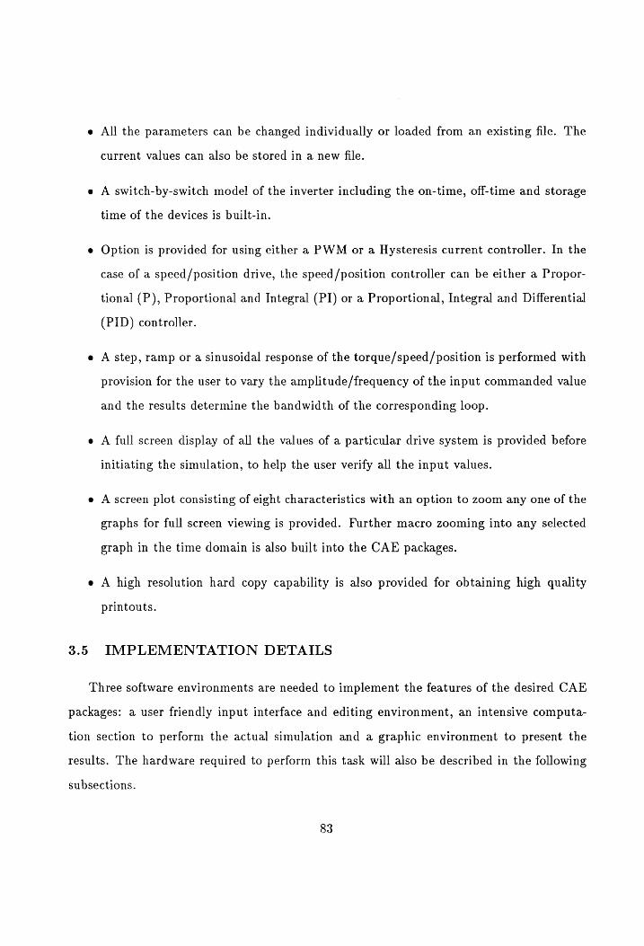
All the parameters can be changed individually or loaded from an existing file. The

current values can also be stored in a new file.

A switch-by-switch model of the inverter including the on-time, off-time and storage

time of the devices is built-in.

Option is provided for using either a PWM or a Hysteresis current controller. In the

case of a speed/position drive, the speed/position controller can be either a Propor-

tional (P), Proportional and Integral (PI) or a Proportional, Integral and Differential

(PID) controller.

A step, ramp or a sinusoidal response of the torque/speed/position is performed with

provision for the user to vary the amplitude/frequency of the input commanded value

and the results determine the bandwidth of the corresponding loop.

A full screen display of all the values of a particular drive system is provided before

initiating the simulation, to help the user verify all the input values.

A screen plot consisting of eight characteristics with an option to zoom any one of the

graphs for full screen viewing is provided. Further macro zooming into any selected

graph in the time domain is also built into the CAE packages.

A high resolution hard copy capability is also provided for obtaining high quality

printouts.

3.5 IMPLEMENTATION DETAILS

Three software environments are needed to implement the features of the desired CAE

packages: a user friendly input interface and editing environment, an intensive computa-

tion section to perform the actual simulation and a graphic environment to present the

results. The hardware required to perform this task will also be described in the following

subsections.

83

3.5.1 Input Environment

The requirements of this module include pop-up windows, multiple help screens, the

ability to input and output data files and the overall control of the program. Pascal was

chosen as the programming language for this task for reasons given below.

Turbo Pascal, with built-in windowing functions, allows the separation of drive system

parameters into several windows and hence a modular structure. This aids the user to

modify specific subsystem parameters. The use of well organized windows and strategically

placed operation information makes the program more user friendly. The last line of the

screen has been reserved in this package for program operation information. This informa-

tion includes a brief description of how to accomplish several tasks such as opening and

closing windows, editing, etc. The user friendly requirement of the CAE package is ac-

complished with full screens of help information, in text or graphic format, available upon

request at almost every stage of the program.

The next requirement is the use of data files to store the parameters of a drive system.

ASCII data files were used so that a user can edit the files with only a text editor. The

user can choose a file to load from a list of available files found in the current sub-directory.

Also, as the specifications are changed, they can be saved to a disk. If the user-specified

file name is being used by another file, the user should be warned and allowed to specify

another file name.

The last requirement is the ability to run other programs from within the current en-

vironment. Choosing the run option creates a temporary file containing the current drive

system parameters. Once the simulation program is executed, control is returned to the

main environment. Advantages of this structure are the ability to continue unaffected af-

ter a simulation program crash, to determine whether the simulation program terminated

normally and to indicate the type of error encountered.

84

3.5.2 Numeric Calculations

This environment performs the calculation of various output characteristics of the drive

system such as speed, torque, currents and voltages. Since several of the algorithms for

simulation have previously been implemented in Fortran, it was selected for this task. The

data is read in from the temporary data file created by the input environment. The cal-

culations are made for each instant of time by solving a system of nonlinear differential

equations using the fourth order Runge-Kutta algorithm. Due to the iterative nature of

this algorithm, the execution speed is of prime importance. Microsoft FORTRAN 5.0 was

used to compile this program because it produced faster codes than several other versions

of Fortran.

The data produced during simulation is available in tabular form for use in the graphic

environment. Due to the resolution limitations of the monitor to display the graphs, and

the memory constraints for the data file, the number of data points output to the data

file is regulated. A limit of 1500 data points has been implemented by writing to the data

file only after a calculated number of iterations have been completed. Thus, the output is

effectively sampled at up to 1500 equal intervals during the simulation.

3.5.3 Graphic Environment

The requirements of this environment include graphic representation of the simulation

results and the ability to read and store those values. A program was developed that

could read the data file created by the simulation package and display the data in eight

graphs on the same screen. By selecting one of the graphs, a full screen display could be

produced. Further magnification along the time axis is also available. This features aids in

the examination of the transients in the simulation results. In addition, a hard copy of the

graphs can be obtained. The user is prompted at the bottom of the screen with all of the

available features.

3.5.4 Hardware

The software was developed on an IBM PS/2 model 50 with a 30 Mb hard drive and an

EGA monitor. The software will run on an IBM PC, XT, AT, PS/2, or any true compatible

that has an EGA or VGA monitor. The hard drive is not a requirement, but due to the

size of the output files and the slow access speed of floppy drives, a hard drive is highly

recommended.

The size of the executable code for all the programs needed for each CAE package that

has been developed is about 1 Mb. A sample data file produced by the simulation module

is about 200 Kb. Therefore, the space recommended to run the software is at least 2 Mb.

This would provide space for several default drive system specification files and more than

one simulation result file.

3.6 RESULTS

The results obtained using the CAE packages are presented and discussed in this section.

The various user-friendly features described in the previous sections are implemented in

these packages. A sample screen containing the interactive windows is illustrated in Fig. 3.6.

It can be noted that each item can be selected by moving the arrow keys and a brief definition

of the item selected is displayed in the WATCH box on the bottom of the screen. A sample

full screen help menu of external reference signals is illustrated earlier in Fig. 3.5. This

feature provides detailed help on a single keystroke and guides through the various options

in the software. This would help a new user to adapt to the package very quickly.

A full screen display of the various parameters of the drive system is displayed before

the actual simulation is performed. This helps the user to check the validity of the drive

system specified and provides an option to modify any of the erroneous values thus saving

simulation time. One such display for a speed drive system is illustrated in Fig. 3.7. The

input to the drive system is the speed command which is maintained at the commanded

value by controlling the set of stator currents. The data screen contains seven groups of

86

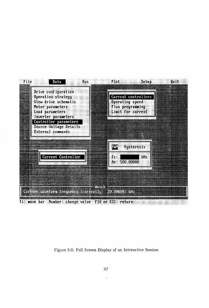
Tho move bar. Number: change value F1i0

Figure 3.6: Full Screen Display of an Interactive Session

87

a aes MU

ad Load ‘Parameters ~

oa -000E +02.

u

otek. 000E+

01 No.

Figure 3.7: Parameter Screen Defining the Drive System

88

data, viz., motor parameters, load parameters, converter parameters, external commands,

time step, controller parameters, flux programming and the base values. Once the user

selects to run the simulation, the iteration steps are displayed on the bottom of the screen.

The graphical output obtained using the speed drive system is shown in Fig. 3.8. For

the torque drive system the normalized values of the actual speed, commanded flux current

and the rotor flux, load torque commanded torque current and the electromagnetic torque,

commanded and actual current of phase ‘A’ are displayed. A sinusoidal command of +1 p.u.

for the electromagnetic torque signal is applied. This is useful in determining the bandwidth

of the overall drive system. The torque response closely follows the commanded signal. A

compressor load is applied and the load profile can be noted from the characteristics. The

decoupled field and torque currents from the vector controller are given with the actual

rotor flux and electromagnetic torque obtained from the drive system. The inner current

loop is represented by the commanded and actual values. The actual current follows the

commanded value of the current, implemented by a PWM controller. The transient and

steady state response of the current can also be seen in this figure.

Fig. 3.9 illustrates the flux trajectory for drive system described here. The g and d axes

rotor flux values are plotted and it can be noted that the orthogonality is maintained by

the circular trajectory. This is an effective tool to verify the decoupling nature of the vector

control strategy.

The temperature and saturation effects of the torque and flux characteristics of a torque

drive are shown in Fig. 3.10. The torque command versus actual torque/flux characteristics,

assuming a constant saturation factor for various slip speeds, is presented in the top two

plots of Fig. 3.10. The parameter a is the temperature factor and is defined as the ratio

of the rotor time constant of the motor and its instrumented value in the vector controller.

The parameter ( is the saturation factor and is defined as the ratio of the actual mutual

inductance and the instrumented value in the vector controller. For a < 1 which signifies

an increase in the rotor temperature, the electromagnetic torque and the rotor flux linkage

is greater than the commanded value. Though the rotor flux is shown to increase beyond

89

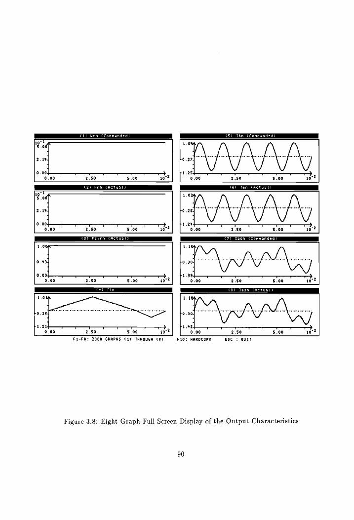
C1) Urn (Conmanded)

107+ 5.0

2.144

0.00 v T T ' tT 7 qT t >,

0.00 2.50 5.00 10

(S) Itn (Commended)

(See ae ote ee)

10°: 5.0

2.184

0.00 T T a T TO v t T >. ri. 244 T T T T >»

0.00 2.50 5.00 10 9.00 2.50 §.00 10

1.0

0.431

0.00 t J ¥ q t t qT T >, r 1.394 Oe tT ' T T vv >,

0.00 2.59 5.00 410 9.00 2.50 5.00 10

Sear (3) Tagn CAactual)

P3234 T T T T T T T —“T >» 8.424 T T T T T T 7.2 0.06 2.50 5.00 10 0.00 2.50 5.00 10

Ft-F8: 200M GRAPHS (1) THROUGH (8) FiO: MAROCOPY Esc : QUIT

Figure 3.8: Eight Graph Full Screen Display of the Output Characteristics

90

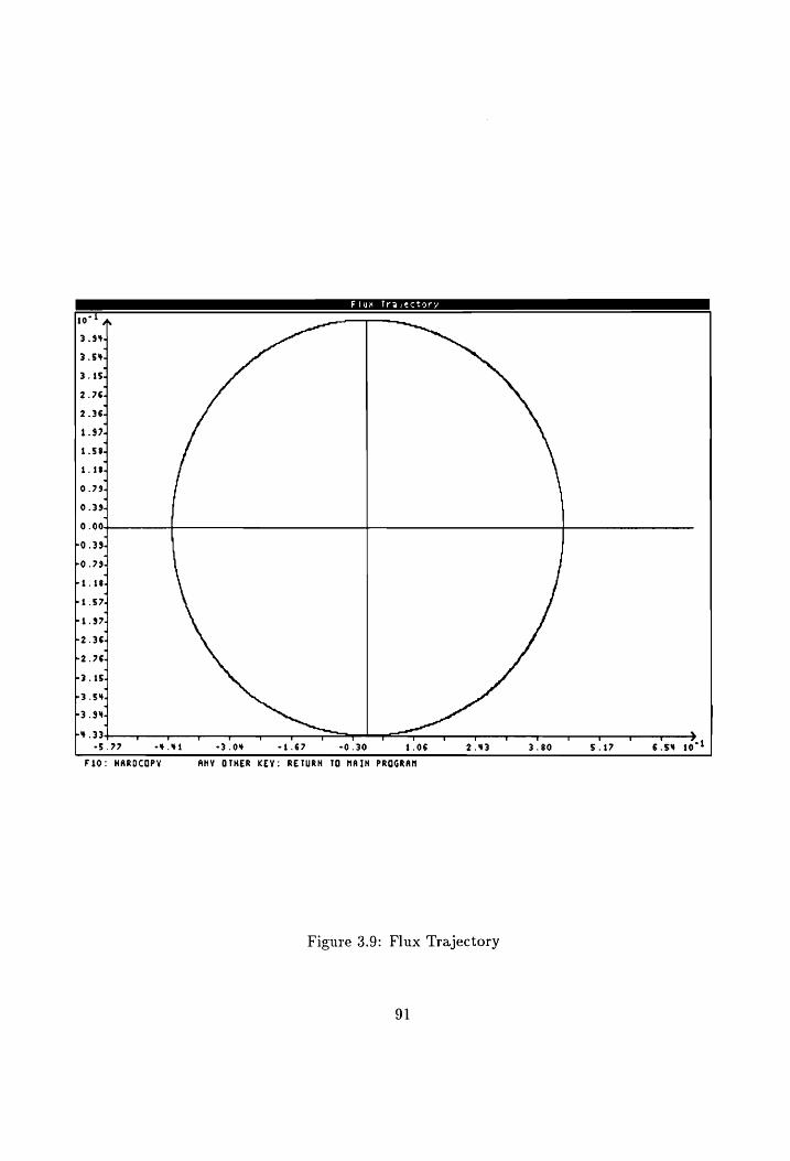
* 944

SH isd

764

364

974

-—

ee

hl rrellUrhlUlUNUlUlUlUMWwOW

oo

8

ws

o i

L039. bo.791 wr? b1.574 Pi .$74

L2 364 b2 .76-

e3.1S4

L3 sw

-3 944 4

PY 33 r r - s ? v v Tt v v T T T t q T t T v &

-5.77 “441 3.04 “1.6? -0.30 1.06 2.43 3.80 5.17 6.s¥ 107! F1i0: KAROCOPY ANY OTHER KEY: RETURN 10 MAIN PROGRAN

Figure 3.9: Flux Trajectory

91

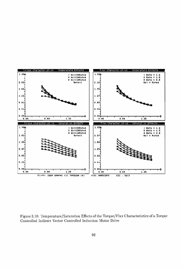
Torque Characteristics Tenperature Effects

Fiun Characteristics . Tenperature Effects

1.8 * Us ls3¥Rated 1.32 * Bets = 1.2 Y Usls2eRated a ¥Y Betas = 1.0 RB UsisiRRated 4 ¥ Beta = 0.8

2.03 Beta=i 2.124 Ust = Rated

1.63 1.704

1.22 1.274

0.8! 0.854

O.44 0.424

6 + ol s 0.004 T v tT t t v To 0.90 v TT tT qT qT t T T ¢

0.00 0.68 1.35 0.00 0.68 1.35

Torque Chsracteristics © Saturation Effects Flum Characteristics © Saturation Effects

1.4% o Wsls3KRated 1.87, * Bets = 1.2 WV Us ls2RRated ¥ Beta = 1.0

KR USISLERIted X Beta = 0.8 1.62 Beta=t 2.07 si = Rated

1.23 1.66

Q.97 1.24

0.65 0.83

0.32 O.41

0.004 t qT t t ' t T > 0.004 T T v v T t >

0.00 0.68 1.35 0.00 0.68 1.35

Fi-F%: 200M GRAPHS (1) THROUGH ($) F100: HAROCOPY Esc : Qurr

Figure 3.10: Temperature/Saturation Effects of the Torque/Flux Characteristics of a Torque

Controlled Indirect Vector Controlled Induction Motor Drive

92

1.2 p.u., it is difficult to maintain this high value due to saturation. An increase in a

indicates an increase in motor saturation at ambient temperature and for such operating

conditions the torque is less than the commanded value. The bottom two plots of Fig. 3.10

illustrate the saturation effects of the torque and flux characteristics. It can be noted

that both the torque and flux values increase when a is less than one and decrease when

@ is greater than one. Hence it can be noted that linearity of the input-output torque

relationship has degraded and the induction motor drive is unsuitable for use in torque

control applications. Either an outer speed loop or a torque loop/parameter compensator

becomes essential to achieve a linear torque amplifier.

The temperature/saturation effects for the torque, flux, slip speed and peak stator

current for a speed drive are illustrated in Fig. 3.11. It can be noted that the torque

and flux follow the commanded values for a = 1, at any rotor speed. With decreasing a

the torque is less than its commanded value up to 0.75 p.u. load torque, beyond which

the actual torque is greater than the commanded value. When a is greater than one the

behavior is just the opposite. The rotor flux decreases for values of a greater than one up

to 0.7 p.u. load torque and then remains constant. At a equals 0.5, the actual value of flux

increases monotonically with the load torque. Due to the saturation of the motor, only a

modest increase in magnitude results.

The slip speed is linear for a = 1, but exhibits other trends for various values of a. For

a less than one, the slip speed is higher than the nominal value up to a reasonable fraction

of full load, beyond which it becomes slightly less than the nominal value. The peak stator

current has a close resemblance to the slip speed characteristics. This trend signifies that

the rotor losses increase for values of load torque less than 0.8 p.u.

The bottom four plots of Fig. 3.11 illustrates the saturation effects for the torque, flux,

slip speed and the peak stator current. As expected, saturation decreases the flux level by

20 percent, while the value of torque is lower than that of the command value. From the

slip speed characteristics, it can be noted that a = 0.5 and around 1 p.u. load torque, the

drive will have lower losses than its nominal value and designed peak capacity, even when

93

Torque Characteristics Temperature Effects Slip Speed Character istics Tenpersture Effects

1.4 2.950 « Alpnasi.s ¥ Alphast.o

¥ Alphasd.s

0.62 1.264 Beta=i

0.004 + t T t r ¥ , T > 0.004 v v v r q t >

0.00 0.78 1.50 0.00 0.78 4.50

Peak Stator Current Chars Tenberature Effects 1.6 5.7

0.70 . x. ws. -. A 2.46

0.004 T SF ' v i T > 0.004 T t v >

0.00 0.75 1.50 0.00 0.75 1.50

Torque Chsractersstics © Saturation Effects Slip speed Characteristics © Saturation Effects

1.6 * Betazi.2 WY Betasi.o ® Betasd .8

0.69 Aiphasd .S

0.004 $ t t T qT T T a > 0.004 iF T t T t r my qT >

0.00 0.78 t.$0 0.00 0.75 1.50

1.3 3.22

0.85 1.39

0.004 qT OE t T ot t > 0 00+ oT T v v ‘ qT t t >

0.00 0.75 1.50 0.00 0.75 1.50

Fi-FS: 200M GRAPHS (1) THROUGH (8) FiO: MAROCOPY esc : Quit

Figure 3.11: Temperature/Saturation Effects of the Steady State Characteristics of a Speed

Controlled Indirect Vector Controlled Induction Motor Drive

94

the saturation effects is included. This is due to the fact that saturation has increased

the peak stator current. The drive operation is usually confined to values of torque 1 p.u.

and lower, and in this region, it can be noted that the stator losses are higher. This is

highly undesirable from the point of view of thermal rating of the motor and the overall

system efficiency. Various other modules such as steady state efficiency, and Fourier spectral

analysis are built into the system and their results help to better understand the overall

drive system.

3.7 DISCUSSION

The methodology for the development of a CAE package for the dynamic analysis of

vector controlled induction motor drive systems is presented. This package would aid in

the assessment of the torque ripple, losses, efficiency, torque, speed, and position responses

and their bandwidth and the suitability of the drive system for a particular application.

Based on this principle, four such packages, VCIM, PMBD, PMSM, and SRMCAD were

developed for the computer simulation of variable speed motor drive systems. This chapter

describes in detail the various subsystems involved in the drive system. The usefulness

of the CAE packages has been emphasized by going through the features incorporated

and the discussion of the results obtained. The development of such CAE packages for

ac drive systems would benefit the drives industry by helping to reduce the development

time and product cost. Even though quite a number of features have been discussed and

implemented in these packages, the author believes that this is just the beginning of research

and development in this area. Future research can be addressed to developing time optimal

algorithms for control, detailed subsystem modeling for increased accuracy, object oriented

coding for multi motor drive systems, and an effort can be made towards the development

of Expert Systems for such tasks.

A number of drive systems for various industrial applications are variable speed drives.

This would lead to the fact that many vector control induction motor drives require the

95

speed controller to maintain a low speed error signal. Hence, care should be taken in the

design of the parameters for the speed controller. The similarity of the vector controlled

induction motor drives and the separately excited dc motor has been stressed earlier. The

large signal model for the design and study of the speed controller parameters has been

presented in [133]. A similar method for the vector controlled induction motor drives

would help reduce the complexity of the design process. This would also lead to enhanced

performance characteristics of the overall drive system. An effort has been made to develop

such an algorithm and would be described in the next chapter. A method to reduce the

overshoot of the rotor speed within allowable limits using this study is also presented.

96

Chapter 4

DESIGN AND STUDY OF THE SPEED

CONTROLLER

4.1 INTRODUCTION

A number of modern manufacturing processes, such as the machine tools require variable

speed drives. The most commonly found applications for the speed controlled motor drive

systems are in steel, textile, paper and pulp, and mining industry. As discussed in the earlier

chapters, vector controlled induction motor drive systems are extensively employed for such

applications. The successful operation of these drives is dependent on the performance of

the speed controller. The proportional plus integral (PI) controller is normally employed to

maintain the error between the commanded and actual values of the rotor speed minimum.

The design of the gain and time constants of the speed controller is of paramount importance

in meeting the dynamic specifications of the motor. The large signal model for the speed

controlled dc motor has been developed earlier and a systematic approach was presented for

the design and study of the speed controller [133]. Such a study would help in improving

the overall response of the drive system. The similarity between the separately excited dc

motor and the vector controlled induction motor drive has been established in the earlier

chapters. By utilizing this similarity, an identical approach for developing the large signal

model would simplify the design of the speed controller and hence improve the overall

response.

This chapter deals with the design and study of the speed controller for an indirect

vector controlled induction motor drive system. The large signal model is formulated for

the indirect vector controlled induction motor drive in the next section. This is followed by

97

a step by step derivation of the transfer function of the overall drive system. A method to

reduce the overshoot of the speed response based on the model developed is also presented

in Section 4.3. The simulation results for the design of a speed controller for a given drive

system using this method is presented in Section 4.4. Section 4.5 presents the experimental

verification obtained using the DSP based setup described earlier, followed by a discussion

of the various issues on this topic.

4.2 MODELING OF THE SPEED CONTROLLED DRIVE

Speed controlled drives, operating only in the constant torque region, are employed in

many applications due to the simplicity of control. In a dc motor drive, this is achieved by

armature control which has the advantage of a faster response compared to that of a field

control which is sluggish. It can also be noted that since the operating speed is always less

than the base speed of the motor, field weakening is not necessary. In other words, the field

current is maintained constant for all operating conditions.

The induction motor has a tachogenerator whose output is utilized for closing the speed

loop. The motor will drive a load which will be assumed to be frictional for the purpose

of this study. The output of the tachogenerator is filtered to remove the ripples to provide

* the rotor speed signal, w,. The speed command, w*, is compared with the actual speed,

w,, to produce a speed error signal. This signal is processed through a speed controller to

determine the torque command. The torque command is limited so as to keep it within

safe allowable limits and the current command is obtained by proper scaling. Since the

field current is maintained constant, the control of the stator phase currents is equivalent to

controlling the torque current in the vector controller. The torque current is obtained from

the electromagnetic torque and the torque constant. The commanded value of the torque

current is compared with the actual torque current so as to have a zero current error. The

current error signal is processed through a current controller to obtain the q axis voltage

or the torque voltage. From the equations of the vector controller, the induction motor

98

drive has been modeled with an inner induced emf loop, similar to that of a dc motor.

The interaction of the emf loop and the inner current loop increases the complexity in the

development of the model.

The inner current loop assures a fast current response and the limiter also maintains

the current to a safe preset level. This inner current loop makes the converter a linear

current amplifier. The outer speed loop ensures that the actual speed is always equal to the

commanded speed and any transient is overcome within the shortest time without exceeding

the motor and converter capabilities. The transfer functions of the various subsystems will

be described in detail in the following subsections.

4.2.1 Induction Motor

The qg and d axes stator voltages of the induction motor in the synchronously rotating

reference frames are given as,

Ups = (Rs + Lsp)ig, + WeLsig, + Lmpty, + Welty, (4.1)

Vis = —Wel sts, + (Rs + Lsp)t4, ~~ We Lis, + LmPtGp (4.2)

But, from the derivation of the vector controller discussed earlier, the following relation-

ships are known,

re tos = Ut

las = ty

bor = 0 (4.3) Vdr = Yr

For this study, since the motor operates in the constant torque region, there is no field

weakening and the field current is constant. Hence,

99

pis =0

py, = 0

The rotor flux and synchronous stator frequency are given as,

Yr = Lmtf

We = Ws + Wy

Also, the g and d axes rotor currents are given as,

gr -_™ 2 ut

-e Vr Lm . lar = L, ~ L, ‘Ff

Lm . Im. = L, 7 L, °F

= 0= Plar

Rewriting the g axis voltage or the torque voltage using the above relationships,

, . 2, 5 (Rs + Lp) te + We L gts — L Prt

— [2 , ; L;L m\_: . Rstz + (SF pit + Wel sts

(Ry + Lap)it + wel siz

e lI II

where,

(4.4)

(4.5)

(4.6)

(4.7)

(4.8)

(4.10)

Hence,

- Ugs —™ Wel sty _ Ugs —_ (w, + Ws) Dsts

er =

* ~ “(Rs + Lap) (Rs + Lap) (4.11)

From the dynamic model of the induction motor, the equations for the slip frequency

and the electromagnetic torque are given as,

o LmRp Ut sl = —{

L, r

_ fir ~ L, Uf

3 P Lm. TT. = 201 tt Yr

3 PL? ... = (Sa L. tf)

= Ket

where KK, is the torque constant, defined as,

ti 3 PL? K-32 Lh,

‘t= 99 7,

The transfer function for the induction motor torque channel is given as,

ii(s) Ka Ga(s) = V.(s) 1+8T,

where, from equation 4.11,

Ve(s) = vf, — weLsis(s) and the gain and time constants are given as,

(4.12)

(4.13)

(4.14)

(4.15)

(4.16)

(4.17)

— (4.18)

4.2.2 Load

The load is modeled as a function of moment of inertia, J, with a viscous friction

coefficient of B. Then the acceleration torque drives the load and is given by,

db Ih

P + Buy = 5(Te ~ Ti) (4.19)

where, 7; is the load torque. The load torque is assumed to be frictional for the purpose

of this study. Hence, the load is proportional to speed and given as,

T) = Biwm (4.20)

The transfer function for the frictional load is given as,

Wr Km n(s) = = = ——— 4.21

Gm(s) Te(s) 1+ 8Tm (4.21)

where the gain and time constants are given as,

- P 1 P\ 1 cs=() xin) am J

Tm = => 4.2:

4.2.3 Current Controller

The most commonly used techniques for current control are the hysteresis and PWM. In

the case of a hysteresis controller, the response is instantaneous and hence the controller is

modeled as a simple gain of unity. For this study, a standard PWM controller is employed

to reduce the current error. The PWM controller has a delay of half the time period of

102

the carrier waveform with a frequency of f,. It can be noted from the block diagram that

the input of the PWM controller is the error torque current, 24¢, in volts, and the output

is the q axis stator voltage in the synchronously rotating reference frames. The maximum

rms voltage of the g-axis voltage under steady state conditions cannot exceed 0.45 X Vac.

The inverter gain can then be represented as a function of the peak voltage capability

corresponding to the available control voltage. Hence its transfer function is given as,

Ug K

G(s)=—“*= < 4.24 (s) tree(S) 1+sT, (4.24)

where

tte($) = tin(S) — ttm(s) (4.25)

and the gain and time constants are given as,

, Vie K, = V2 x 0.45 x —% (4.26) Vo

T.=— (4.27) © fe

where V, is the control voltage and, f, is the switching frequency of the PWM controller.

4.2.4 Speed Controller

The proportional plus integral (PI) controller is the most commonly used technique for

the speed controller. It consists of proportional and integral gain constants. The speed

controller to calculate the torque command for any speed error signal is:

Ty = Kyl} —w,) + Ki [ (wt - wy) at (4.28)

where, A, and K; are the proportional, and integral gain constants, respectively. The

transfer function of the speed controller is given as,

103

K,(1+ sT, G(s) = BOF 8h) (4.29) where the gain and time constants are given as,

K, = K, (4.30)

K

T, = — (4.31)

4.2.5 Speed Feedback

Most of the high performance drives use a dc tachogenerator and the filter required is

a low pass with a time constant of 2 msec. or less. The transfer function of the feedback

filter is given as,

Wrm(s) _ Ky

ws) 14+ s8T, H(s) = (4.32)

where J, is the gain and T,, is the time constant of the dc tachogenerator and filter.

4.33 OVERALL TRANSFER FUNCTION EVALUATION

The step by step derivation of the overall transfer function of the drive system is given

in Fig. 4.1. The equations for the motor are incorporated in the induction motor, EMF

calculator, and slip speed calculator blocks in the figure. By including the slip speed cal-

culator into the motor model and simplifying the loop, the new transfer function is given

as,

ir(s) _ Ky

Vos — W, Lsts 14 8T; Gp(s) = (4.33)

where the gain and time constants are given as,

104

RD, ” ”

Ky = Ky / ( + Ti) = Ka [K; (4.34)

T, T == 4.35 = (4.35)

The following are the transfer functions defined in the step (iv) of the block diagram

reduction, given in Fig. 4.1:

W)= Bytom a (436)

G(s) = OI = F (4.37)

G3(s) = e, A = 7 aS (4.38)

G4(s) = ae = 4 a“ (4.39)

A(s) = ont ~ rs ST. (4.40) By further reduction and arriving at step (vi) as shown in the figure,

Gs(s) = G2(s)Ga(s) (4.41) ~— 14+ Gs(s)G4(s)KyL sis

Similar to the derivation of the transfer function of the dc motor, the second order model

of the current loop is replaced with an approximate first order model to design the speed

loop. This helps to reduce the order of the overall speed loop gain function. This leads to

the approximation of the following transfer function,

KK K, G2(s)Ga(s) = (i+sT.)(1+sT) 14sT, (4.42)

105

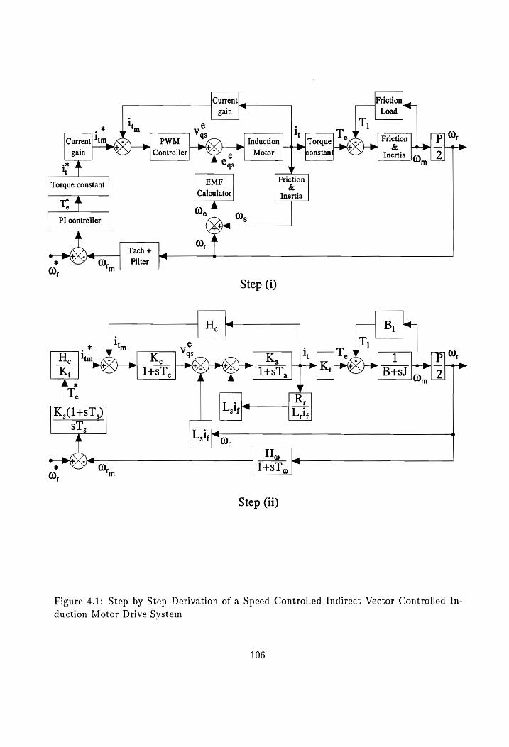
Current Friction

gain Load

e : q : Vv 1, T a

Current 48 Induction Torque| © Prignon P OC gain Controller e Motor constant Inertia ® 2

.* gs m

T EMF Friction orque constant

Calculator Inertia

TS PI controller

¢ , Tach +

* 0), Filter

@), m

Step (1)

<< H, B,

ve . q qs K, | |* qT, 1 P| or + + > K pT oT sree 1+sT, t B+sJ @,, -2

Li —_—_| Br K,G+sT,) sl Li

sT, Lig} s*f 0,

im

* @ 1+sT ©, =

Step (ii)

Figure 4.1: Step by Step Derivation of a Speed Controlled Indirect Vector Controlled In-

duction Motor Drive System

106

H,K,(+sT,) i K, | Vos K,] |i -KK,)] ® KysT, 1+sT, 1+sT, 1+sT,,

ea

Laie =

* H ©

, QO, 1+sT,,

Step (iii)

H,

as iy ®, G,(s) G,(s) K,G,(s)

e Eqs

Lip

W, Q, H(s)

Step (iv)

Figure 4.1: Step by Step Derivation of a Speed Controlled Indirect Vector Controlled

107

Induction Motor Drive System

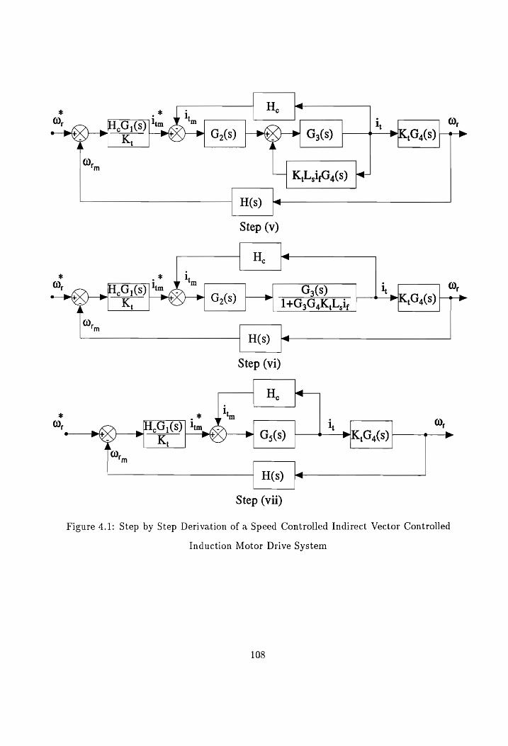
eGy(8)]"™ S ™ i, 0, “ee G,(s) © G,(s) K,G,(s)

0,

—| KLi,G,(s)

H(s)

Step (v)

H, \

* Ji ; ~Gy(s)] "= G,(s) I, O, K, G(s) 1+G,G,K Lj; K,G,(s)

QO,

H(s)

Step (vi)

H, +—

it Q, G,(s) K,G,(s) >

0,

H(s)

Step (vii)

Induction Motor Drive System

108

Figure 4.1: Step by Step Derivation of a Speed Controlled Indirect Vector Controlled

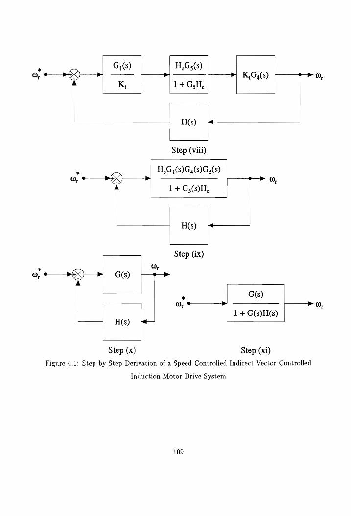
* G,(s) H,G,(s) . 0), > > K,G,(s) Q,

K, 1+ GsH,

H(s)

Step (viii)

H,G,(s)G,4(s)G;(s) o, s+) > > 0,

1 + G;(s)H,

H(s) -~————

Step (ix)

* O, Q, G(s)

‘ G(s) w, © > PO,

1 + G(s)H(s)

H(s)

Step (x) Step (xi)

Figure 4.1: Step by Step Derivation of a Speed Controlled Indirect Vector Controlled

Induction Motor Drive System

109

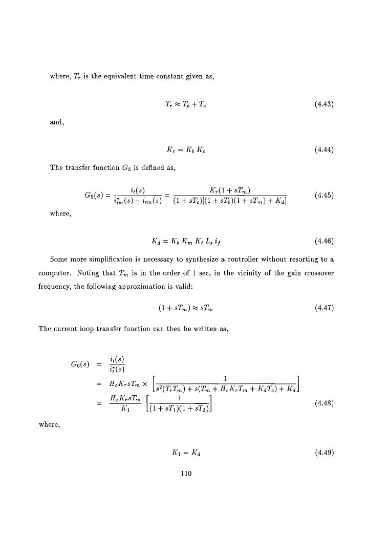
where, JT, is the equivalent time constant given as,

T, = Ty + Te (4.43)

and,

K, = K, K- (4.44)

The transfer function Gs is defined as,

iz(s) K,(1 + sTm) Gs(s) = - - = : 4.45

5(8) (3) —tem(s) (1+ sT.)[(1 + 8T)(1 + sTm) + Ka] ( )

where,

Ky = Ky Ky Ky Ls ts (4.46)

Some more simplification is necessary to synthesize a controller without resorting to a

computer. Noting that T;,, is in the order of 1 sec, in the vicinity of the gain crossover

frequency, the following approximation is valid:

(1+ sTn) & sTm (4.47)

The current loop transfer function can then be written as,

“0 =

1 = c+ sTm ; HeKssim x SET + 5(Tm + HeK; Tm + KaTs) + Ka

A.K,sTm | 1 = > 4.48

Ky (1 + sT;)(1 + sT2) ( )

where,

Kk, = Kg (4.49)

110

—2T,Tm

T= 4.50 ‘Lb — J? — 4K TT (4.50)

—_ T; m Ty = oT Tm (4.51) b+ /b? —4K,T.T,,

and

b= Tn + HeK-Tm +T.Ka (4.52)

Since the value of 7; is much greater than that of TJ, and in the order of 1 sec, the

following approximation in the vicinity of the gain crossover frequency is valid:

(1 + ST) ~ sT5 (4.53)

The current loop transfer function taking into account this approximation can then be

written as,

cay =

HeK,Tm 1 = 4.54

Kal» fr + a ( 9 )

Hence, the overall open loop transfer function is given as,

AeKmK,K, | (1+ sT;) | = 4, G(s) Kal, |s°T,(148Ti) (4.55)

The loop gain function is given as,

KmK,H.H. K(1 + sT;) | 1 | ivf

GH(s) KaT2 s*T, (1 + sT,)(1 + sT.)

, Ks f (14+sT;) |

82 sr steoy (4.56)

111

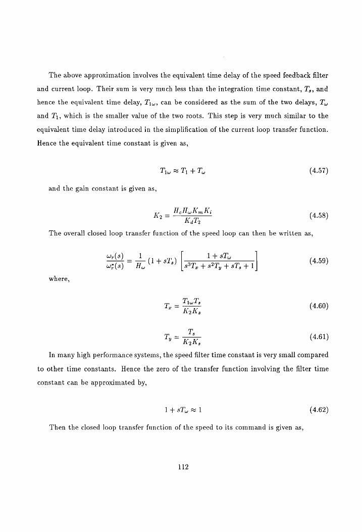
The above approximation involves the equivalent time delay of the speed feedback filter

and current loop. Their sum is very much less than the integration time constant, T,, and

hence the equivalent time delay, T\,,, can be considered as the sum of the two delays, T,,

and 7;, which is the smaller value of the two roots. This step is very much similar to the

equivalent time delay introduced in the simplification of the current loop transfer function.

Hence the equivalent time constant is given as,

Ty, ~ Ty + Ty (4.57)

and the gain constant is given as,

AA K mK; K = c Ww m t 4.58

"? KaTy (4-58) The overall closed loop transfer function of the speed loop can then be written as,

w,(s) 1 1+ sT,, _ 4, w*(s) Ay (1+ 875) s3T, + s*Ty +sT, +1 (4.59)

where,

Tw Ts a 4,

Kok, (4.60)

T’ _ s 4.61 Ty Kok, ( )

In many high performance systems, the speed filter time constant is very small compared

to other time constants. Hence the zero of the transfer function involving the filter time

constant can be approximated by,

1+sT, #1 (4.62)

Then the closed loop transfer function of the speed to its command is given as,

112

Wy 1 — = —(1+sT, w* zc (1 + sTs) pea

_ 1 ag + a4

OA ; dg + 418 + azs? + =a (4.63)

where,

ao = 1 (4.64)

a, = T; (4.65)

T; a2 = Tok, (4.66)

Ti T's — 4, “3 TKK, (4.67)

For optimal response, the magnitude of the frequency response is to be as close as

possible to a value of one over a wide frequency range which guarantees a high bandwidth

and hence faster response. The magnitude of the function in the j-domain is given as,

az wW a2 Fiw)| = ot oat (4.68) az + w?(a? — 2apa2) + w4(a2 — 2a,a3) + w%a3

This is optimized by making the coefficients of w? and w‘ zero which yields the following

conditions:

a? = 2aga2 (4.69)

az = 2a,a3 (4.70)

Substituting these conditions in terms of the motor and controller parameters given in

4.64 - 4.67,

Ti = 4.71 °K, Ke (4.71)

113

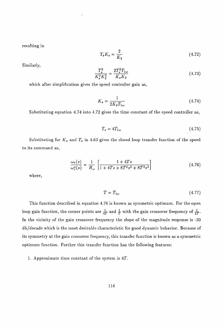
resulting in

2 T; Ks = Ke (4.72)

Similarly,

T2 —2T?T,

— 4.73 K?k? KK (4.73)

which after simplification gives the speed controller gain as,

K,= ! (4.74) * WKoT

Substituting equation 4.74 into 4.72 gives the time constant of the speed controller as,

T, = 4Tw (4.75)

Substituting for i’, and T; in 4.63 gives the closed loop transfer function of the speed

to its command as,

w,(s) 1 1+4+4Ts

w*(s) HAH, |1+47Ts + 8T?s? + 8T3s3 (4.76)

where,

T = The (4.77)

This function described in equation 4.76 is known as symmetric optimum. For the open

loop gain function, the corner points are or and 7 with the gain crossover frequency of oT

In the vicinity of the gain crossover frequency the slope of the magnitude response is -20

db/decade which is the most desirable characteristic for good dynamic behavior. Because of

its symmetry at the gain crossover frequency, this transfer function is known as a symmetric

optimum function. Further this transfer function has the following features:

1. Approximate time constant of the system is 47’.

114

2. The step response is given by,

fopt(t) = on 26 cos( ae vat) (4.78)

with a rise time of 3.17, maximum overshoot of 43.4% and a settling time of 16.57.

3. Since the overshoot is high, it can be reduced by compensating for its cause, the zero

by a pole in the speed command path as shown in the Fig. 4.2. The resulting transfer

function of the speed to its command is,

wr(s) 1 1

w(s) A, i +47 s + 872s? + 7s (4.79)

The step response for this modified transfer function is given as,

foptm(t) = z h — t/t _ See UT sin vat ] (4.80)

with a rise time of 7.67, maximum overshoot of 8.1% and a settling time of 13.3T.

Even though the rise time has increased, the overshoot has been reduced to approxi-

mately 20% of its previous value and the settling time has come down by 19%.

4. The poles of the transfer function are,

_ 1-1 , iv3 ~ 97 47 ~ aT (4.81)

As the real part of the poles are negative and since there are no repeated poles at the

origin, the system is asymptotically stable. Hence in the symmetric optimum design,

the system stability is guaranteed and there is no need to check for it in the design

process.

5. Symmetric optimum eliminates the effects due to the disturbance very rapidly com-

pared to other optimum techniques employed in practical systems such as linear and

115

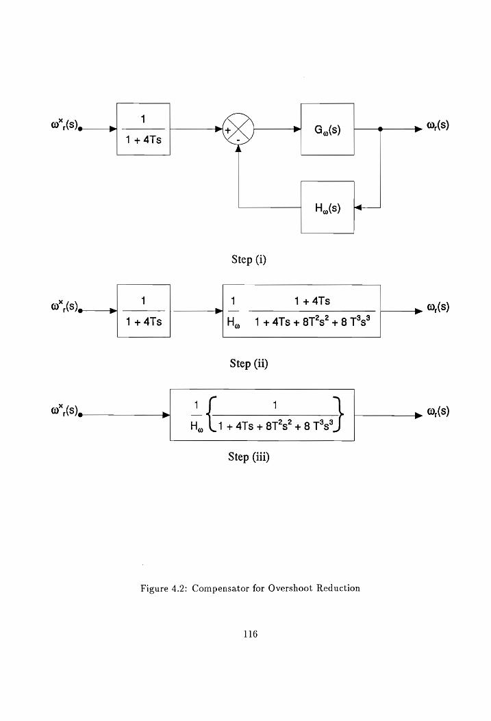
1

@"(S), sg G,(s) @,(S)

1+4Ts

H,(s)

Step (i)

w” (s) 1 » a 1+4Ts > @,(S)

1+4Ts H, 1+41s+8T’s*? +8 T%s°

Step (ii)

w*(S)¢ > i { ' _p ©,(S) H, 1+ 4Ts + 8T’s* + 8 T’s®

Step (iii)

Figure 4.2: Compensator for Overshoot Reduction

116

modulus optimum etc. This approach indicates one of the possible methods to syn-

thesize the speed controller. The judicious choice of approximations is based on the

physical constants of the motor, converter and transducer gains and delays is to be

emphasized here.

4.4 SIMULATION RESULTS

The results which are presented in this section are obtained for the motor drive system

described by the following parameters. The induction motor operates in the constant flux

region and its ratings are LHP, 220V, 2 pole, 60 Hz., 3450RPM, Y-connected motor. The

motor parameters are given in appendix A. A dc motor coupled to the induction motor pro-

vides a constant load of 0.4707 Nm. The rated flux of the motor, ,, is 0.363 Wb.Trns and

the rated torque, T., is calculated to be 1.744 Nm. For the purpose of this study, the PWM

converter is supplied from a dc supply with a dc link voltage of 100 V. The maximum control

input voltage is + 5V. The tachogenerator has a transfer function G,(s) = (4 00038)"

The speed reference voltage has a maximum of 5V. The current limit in the system is set

to 8A.

The dc link voltage, Vy, is given as,

Vice = 100V

The rated voltage required by the motor is 230V. Hence the maximum safe control voltage

is 5V and this has to correspond to the maximum current error, i.e. tmaz

1 max = 8A

H, = Ve ’maz

ee)

~ 8 = 0.625V/A

117

The gain and time constant of the PWM inverter are given as,

Vie K. = V2x0.45 x

0.6364 x 100

5

= 12.728

1

2x fe 1

2 x 1000

0.5 msec

The transfer function of the converter is given as,

12.73

Gels) = Gy 9.00055)

The equivalent inductance of the motor is given as,

L,L, — L?,

Ly = 0.06524H

La

The gain and time constant of the induction motor are given as,

———

I! © ~ o>

—

an

an

7 = — Rs 0.06524

2.1667

= 0.03634 sec

The transfer function of the induction motor is given as,

0.4615

Gals) = 9.036345)

118

The torque constant of the motor is calculated as,

The field current is given as,

3 P Lm K, = ~-2™d, t DD L,Y

= 0.451

, vr = = 1.724A

> TL The gain and time constant of the load for no load conditions, i.e., B; = 0, are given as,

Pol 2B+B,

= 648.09

Km =

B+ B,

= 2.676 sec

The transfer function of the load is given as,

648.09 Gin oS) = 7a rae () = G4 2.6765)

Proceeding further with the block diagram simplification, the following values are calculated.

T;

Ti Ww

T2

Ko

6.48 msec

7, + T,, = 6.48 + 2 = 8.48 msec

0.2759 sec

HoKmKyHy _ 0.625 x 648.09 x 3.31 x 0.01166 _ | oo,

KaT» ~ 31.414 x 0.2759 ——_

Ti. = 8.48 msec

4T = 4 x 0.008484 = 0.0339 sec

2 2 = = 32.681

KeT, 1.803 x 0.0339

Ks, 32.681 = = 963.032

T; 0.0339 963.05

119

Hence, the symmetric optimum function is given as,

G(s) = ( 1 )| 1 + 0.0339s

0.01166/ 1+ 0.0339s + 5.76 x 1074s? + 4.885 x 1076s?

The frequency and time domain responses of the speed to its command without the

compensator is shown in Fig. 4.3. It can be noted that the function closely follows the

characteristics of the symmetric optimum function. The maximum overshoot can be reduced

by adding a compensator for the speed command as discussed earlier. The smoothing of the

overshoot with the cancellation of the zero with a pole at ar is shown in Fig. 4.4. It should

be noted that such a close correlation of the time domain response is achieved if there is

no limit on the torque produced in the motor, since a linear relationship between the speed

error and the torque is assumed. But in practical drive systems, the torque capability of

the motor limits the maximum allowable torque and the small and large signal response of

such a system is considered for the study.

The proportional and integral constants designed using the symmetric optimum tech-

nique is incorporated into the CAE package, VCIM, and the drive system is defined by

the corresponding parameters. The small signal response of the drive system is studied by

applying a 0.02 p.u. speed command from standstill. This condition is equivalent to that

of a 2% perturbation of the input signal. The time domain characteristics is presented in

Fig. 4.5. It can be noted that there is a close correlation of the response obtained with the

linear model. There is an increase in the settling time of the speed due to the fact that the

maximum torque allowed is limited to 1 p.u. The limiter function can be observed from the

behavior of the actual torque response in the characteristic.

The performance of the controller for wide load torque variations is illustrated in Fig. 4.6.

The motor drive system is allowed to reach steady state and then a load torque disturbance

of +0.5 p.u. is applied. It can be noted from the figure that there is only a minor variation

in the actual speed value for such a wide range of load torque variation. This response is

helpful in determining the integrity of the controller.

The overshoot of the response can be smoothed by the cancellation of the zero in the

120

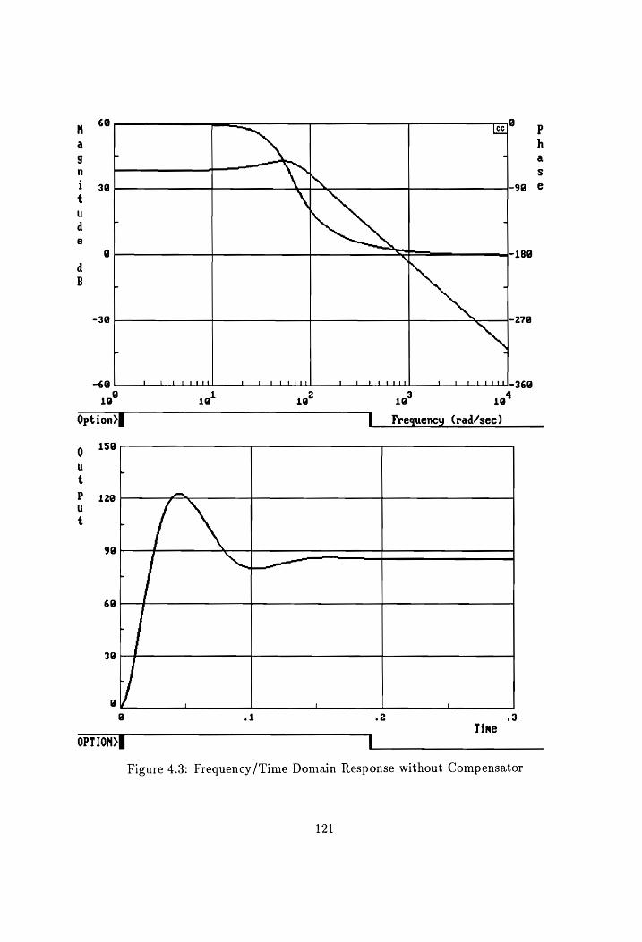
anew

=

9

H 68 we @

a

J i ] n

i 3@ Ap -98

u d L

e @ x2 ~18¢

d

B a Z

-3@ Ny

~69 ___t l Lite | \ Liygitt j | L Eerie 4 \ Liiitis._£369

18° ie! 10° 10° 10°

Option] 1 Frequency (rad/sec)

0 13@

u Pm

t

P 120 += u t a

98 a

6a

30

@ \ _i \

a wl 3 Tine

OPTION, |

Figure 4.3: Frequency/Time Domain Response without Compensator

121

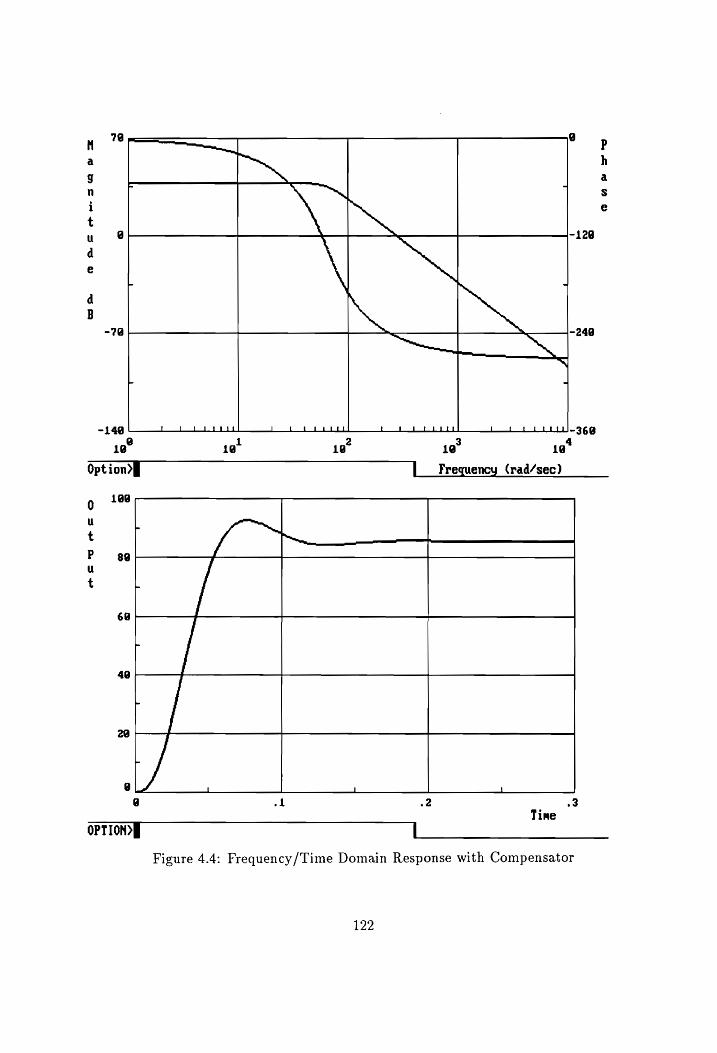
78 @

| AON .

ona Sethe SQW

=

7 / -248

oN -149 a | ! Lopes a Lk tt tl l Ld | L Ltt tt -368

18 16 18 10 18

Option] | _ Frequency (rad/sec)

10

oe

UW et S&S

68

4a

@ al .2 3

Time

OPTION, l

aanmw so

Figure 4.4: Frequency/Time Domain Response with Compensator

122

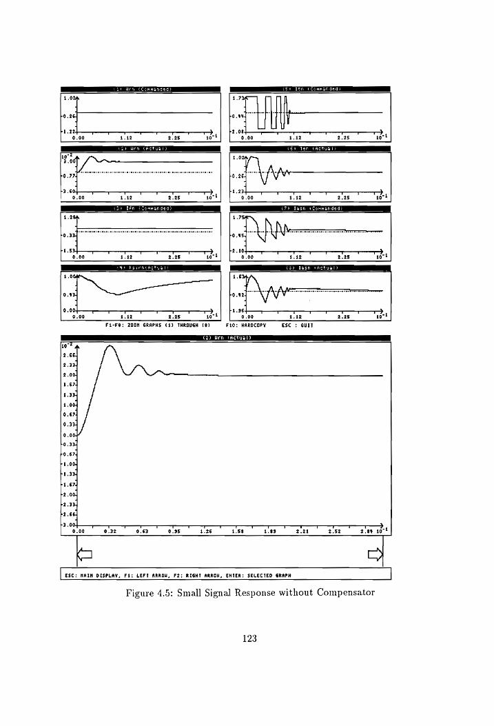
ere (Sa tn (Commanded)

a en oe te Sd

ee eee ee

4 fron 0.4 Lo. #24

0,00 . hi ac! overt t t tT 4 7 T 7 7 Fed oa F t 3 v 7 t Y ed

0.00 21.12 2.25 10 0,00 1.12 2,25 10

FL-F@: 200M GRAPHS (1) THROUGH ($) Fi0: HAROCOPY ESC : QUIT

PP aaa

1072

2.6

2.3

2.0

1.67

1.3

1.0

6.67

0.3

—__-5, T TT “Tt Tt T T T T 7.3

0.00 9.32 0.63 0.38 1.26 1.58 1.39 2.21 2.52 2.8% 10

= Y ESC: MAIM DISPLAY, Fi: LEFT ARROW, F2:; RIGHT ARROW, ENTER: SELECTED GRAPH |

Figure 4.5: Small Signal Response without Compensator

123

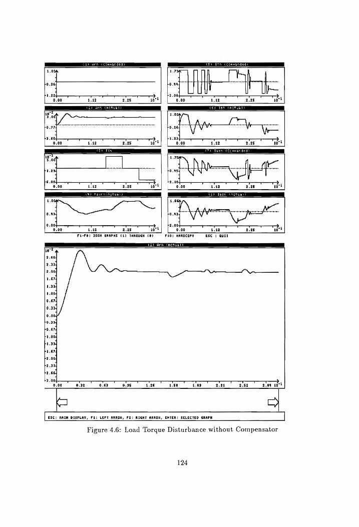
eee eee toa Ith Coma a ded)

1.024

r0.26

pi.22 T T T — T T T a 0.90 4.42 2.28 10

a ea ee ce ee od.

P3 .604— T t T T T TT T > 0.00 2.12 2.25 10

19°! A

CVT ee See See ke

o.% PO .4%3-

0.00 nN Le 00 —\ “I T T T T T T 7 TH he TT ™—T T —T T 0.00 1.12 2.25 10 0.00 1.42 2.28 10

FL-F@: 2008 GRAPHS (4) THROUGH (¢> FiO: HAROCOPY Esc : Quit

(PS Ue ond ee

+300 — -> t “TT —T T Tt T 74 9.00 0.32 0.63 6.35 1.26 1.58 1.39 2.21 2.52 2.84% 10

or o ESC: MAIM DISPLAY, Fi: LEFT ARROW, F2: RIGHT ARKOH, ENTER: SELECTEO GRAPH |

Figure 4.6: Load Torque Disturbance without Compensator

124

symmetric optimum function. This is equivalent to that of a soft start of the drive system.

The small signal response of the drive system is studied by applying a 0.02 p.u. speed

command from standstill with the soft start feature. The time domain characteristics is

presented in Fig. 4.7. The close correlation of the response to that of the linear model can

be observed. There is a considerable decrease in the peak overshoot and the settling time

of the system compared to that without a compensator, as expected.

The performance of the controller for wide load torque variations with the compensator

is illustrated in Fig. 4.8. Similar to the study performed without the compensator, the

motor drive system is allowed to reach steady state and then a load torque disturbance of

+0.5 p.u. is applied. It can be noted from the figure that there is minimal variation in the

actual speed value for such a wide range of load torque variation.

The sensitivity of the drive system to parameter variations is studied for the speed

controller using the symmetric optimum technique. As discussed in the earlier chapters,

the indirect vector control strategy is sensitive to variations in the rotor resistance, R,,

and the mutual inductance, L,. Fig. 4.9 illustrates the large signal drive response for a

100% variation in the value of rotor resistance. The simulation results presented are for a

damping factor of 0.5 without the compensator. It can be noted that there is only a minor

difference in the peak overshoot value when compared to Fig. 4.12. The rise time and the

settling time for both the cases are equal.

Fig. 4.10 illustrates the response of the drive system for a 80% variation of the mutual

inductance value. It can be noted that there is a considerable decrease in the peak overshoot

of the speed response and consequently an increase in the rise time and the settling time

when compared to Fig. 4.12. On the contrary, when the mutual inductance is increased to

120% of its original value, there is an increase in the overshoot and decrease in the rise time

and settling time, as shown in Fig. 4.11.

125

eae ar ee

(Sy Itn tCommanded)

Pa ee ea Te eo

Co) Tesn (Actual)

0.00. —_+ 5 Uy T T TT TT TT T T T T T T, 0.00 1.132 2.25 io 1.12 2.25 10

Fi-F@: 200M GRAPHS (4) THROUGH (8) Fido: HAROCOPY Esc : Quit

eee Ce a

2.0

1.7

4.5

1.2

1.0

0.7

0.5

0.2

0.0

ro.2

ro.5

PO .7

ft -0

pi.2

pi.s

rts?

r2.0

2.284 ne ee — T T T T Tr T > 0.00 0.32 0.€3 o.95 1.26 41.58 1.88 2.24 2.52 2.84 490

— YD | ESC: MAIN DISPLAY, F%: LEFT ARROW, F2: RIGHT ARROW, ENTER: SELECTED GRAPH

el

Figure 4.7: Small Signal Response with Compensator

126

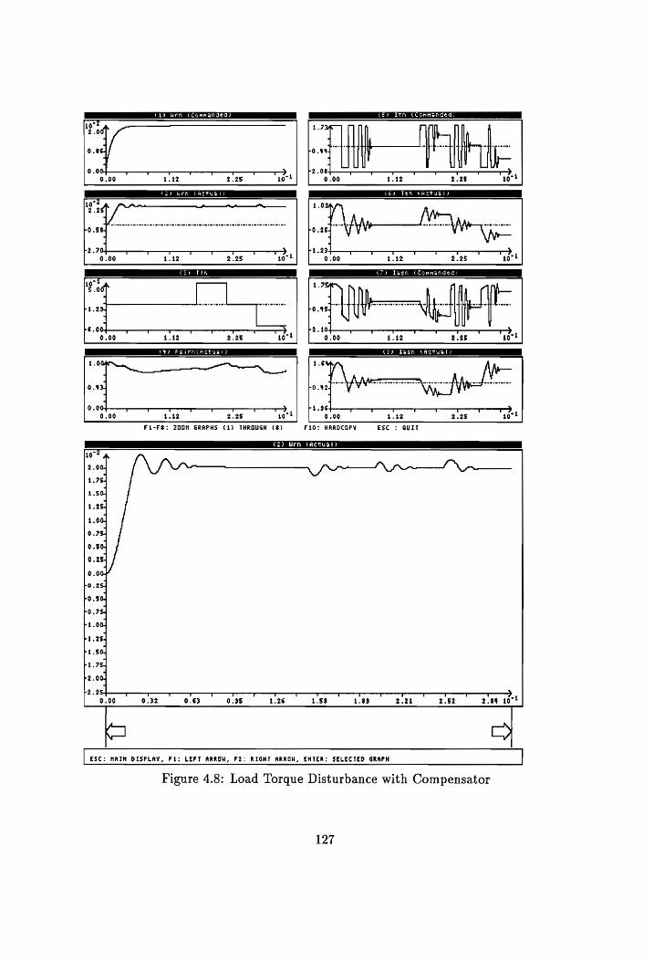
(2) Urn (Commanded)

10 2.0

0.8

0.004 T T T T T 7,

6.00 1.12 2.25 10

iS ee

pe en

Pi .234

Le 00 0.00

T t ¥ t T 1

i 2.25 ion!

4.0

0.8

0.004 9.00

4) Feirntactual) ————

py 12

T f t t i T t vo

1.12 2.25 190

Lo.¥2d

4 a 6 x 1.3 T ft T T v T T T vel

9.00 1.32 2.25 49

FL-FS: 200M GRAPHS (1) THROUGH (3)

[Poe ae Ch

Fi0: HARDCOPY Ese : Quit

Le

| esc: MAIN DISPLAY, Fi: LEFY ARROW, F2: RIGHT ARRON, ENTER: SELECTED GRAPH

Figure 4.8: Load Torque Disturbance with Compensator

127

C1) Urn (Commanded)

See eee

19 *

1.28% 1.226

+0 .334 ~ bO 324

P$.S% T T v T t > ri .47 v ai T T T r UE ay >

0.00 3.75 7.93 0.00 3.78 7.49

10° . 87, +.off a 0.8% 4

hi .034 Lo.22t 1 4

r% 84 T T ™ T > ri.0% T T rT T > 0.90 3.78 7.49 0.00 3.75 7.49

(3) fn (Commanded) 1.70 1.2

bo. 454 O31

4

r2.08 tr T t T a Tr re — ri. E44 t 3 T T T v oF T >

0.00 3.78 7.99 0.00 3.78 7.49

- Dm | ig. 1.4

&.28 ° 37

0.004 T t T t v —_ pi.71+ TE oF r F ' ¥ Tw >

0.00 3.75 7.49 0.00 3.75 7.49 FLcFS: ZOOM GRAPHS (1) THROUGH (8) FiO: HARDCOPY Esc : Quit

LPS Tail ee o_o

| ESC: MAIN DISPLAY, Fi: LEFT ARROW, F2: RIGHT ARROW, ENTER: SELECTED GRAPH

Figure 4.9: Parameter Sensitivity Study: 100% Rotor Resistance Variation

128

(SS ase Lr eek xe)

1.2&H q

bO 334 ~ q

e

ri.5e r 7 t —T mH 0.00 3.75 7.43

CS) Ttn (Commanded)

ae

-

Pt .47 T T "T T ——>

0.00 3.75 7.48

10° 3.6ff

T a“ ws mr y

0.00 3.75 7.49

7.49

C3) Tfn (Commanded)

1.79%

C7?) Tegn (Commanded)

19° A

3.234 4

2.934 o

2.924

ro .%6 +

4

r2.a5 T T T T > Pi. T Tv T T T T T —r>

0.00 3.75 7.49 9.00 3.95 7.49

rT 1.42,

%.2 rO.38

6.004 T T T T T T T — 1.774 T T T T T T?

9.90 3.75 7.%9 9.00 3.75 7.49

Fi-FS: 2O0M GRAPHS (1) THROUGH (8) Fi0: MARDCOPY Esc : Quit

€2) Urn (Actual)

ESC: MAIM DISPLAY, Fi: LEFT ARRON, F2: RIGHT ARROW, ENTER: SELECTED GRAPH

Figure 4.10: Parameter Sensitivity Study: 80% Mutual Inductance Variation

L__}

129

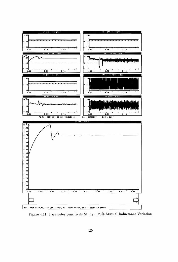
Se ae er lec

1.28%

4

PO .334

ri .5% EE t T 77 0.00 3.75 7.49

Cf) Ttn CCommanded)

1.226

+0 324

Ps.47 OE T T ' v T v =

0.00 3.75 7.49

7-2 ee te 2

0.9%

| oretmreerereteresere: a retereswcwteretererereteseterereseteretes Lo ast TT

5 08! y OF v tT T tO oF T T —F tT v t vt O¢

3.75 7.49 0.00 3.95 7.49

(3) Lén (Commanded) C7) Tagn (Commanded)

1.5 1.2

Lo sgh CUT rrr terete eteretererererereres Lost

4 4

1.86 T T T t > 1.4% t v >

0.00 3.78 7.49 6.60 3.75 7.49

CIMFEAIGSITD ig? 1.57

&.28. eQ.

9.004 T T T T T — Pi.834+——__- >

0.00 3.75 7.49

Fi-F%: ZOOM GRAPHS ¢€¢) THROUGH (9) Fi0: HAROCOPY esc : auit

(2) Urn (Actual) Fn

19

w

ESC: MAIM DISPLAY, Fi: LEFT ARROW, F2: RIGHT ARROW, ENTER: SELECTED GRAPK

Figure 4.11: Parameter Sensitivity Study: 120% Mutual Inductance Variation

130

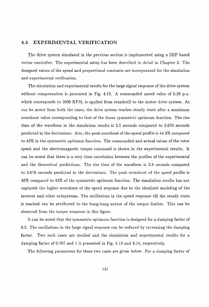
4.5 EXPERIMENTAL VERIFICATION

The drive system simulated in the previous section is implemented using a DSP based

vector controller. The experimental setup has been described in detail in Chapter 2. The

designed values of the speed and proportional constants are incorporated for the simulation

and experimental verification.

The simulation and experimental results for the large signal response of the drive system

without compensation is presented in Fig. 4.12. A commanded speed value of 0.28 p.u.

which corresponds to 1000 RPM, is applied from standstill to the motor drive system. As

can be noted from both the cases, the drive system reaches steady state after a maximum

overshoot value corresponding to that of the linear symmetric optimum function. The rise

time of the waveform in the simulation results is 2.5 seconds compared to 2.676 seconds

predicted in the derivations. Also, the peak overshoot of the speed profile is 44.3% compared

to 43% in the symmetric optimum function. The commanded and actual values of the rotor

speed and the electromagnetic torque command is shown in the experimental results. It

can be noted that there is a very close correlation between the profiles of the experimental

and the theoretical predictions. The rise time of the waveform is 2.8 seconds compared

to 2.676 seconds predicted in the derivations. The peak overshoot of the speed profile is

48% compared to 43% of the symmetric optimum function. The simulation results has not

captured the higher overshoot of the speed response due to the idealized modeling of the

inverter and other subsystems. The oscillations in the speed response till the steady state

is reached can be attributed to the bang-bang nature of the torque limiter. This can be

observed from the torque response in this figure.

It can be noted that the symmetric optimum function is designed for a damping factor of

0.5. The oscillations in the large signal response can be reduced by increasing the damping

factor. Two such cases are studied and the simulation and experimental results for a

damping factor of 0.707 and 1 is presented in Fig. 4.13 and 4.14, respectively.

The following parameters for these two cases are given below. For a damping factor of

131

5 1440 a >3 1260

Cc

= 1080

900 o Oo Actual speed, RPM (sim.) 3 7/20 0 Torque command, p.u. (sim.) oO A Speed command, RPM L ? Actucl speed, RPM (exp.)

fas 540 Torque command, p.u. (exp.)

> Scale: 100 = 1 p.u.Torque command = = 360 ~~ > 180 _ o &

a 0 WY L

~180 ! . . . —_ 0.0 2.2 4.4 6.6 8.8 11.0

Time (sec.)

Figure 4.12: Simulation/Experimental Results of Large Signal Response without Compen-

sator: Damping factor = 0.5

132

1620

3 1440 = 1260

Cc 5

¢ 1080

= 900 oO

S 720 o .

© 540 > §

= 360 Or

oO 180 ®

o 0 YW) :

—180 0.0

(p » th)

Actual speed, RPM (sim.) Torque command, p.u. (sim.) Speed command, RPM Actual speed, RPM (exp.) Torque command, p.u. (exp.) +

orOo

Scale: 100 = 1 p.u.Torque command

. [pees ete etre

i ! 1 l L ! _____} j

2.2 4.4 6.6 8.8 11.0 Time (sec.)

Figure 4.13: Simulation/Experimental Results of Large Signal Response without Compen-

sator: Damping factor = 0.707

133

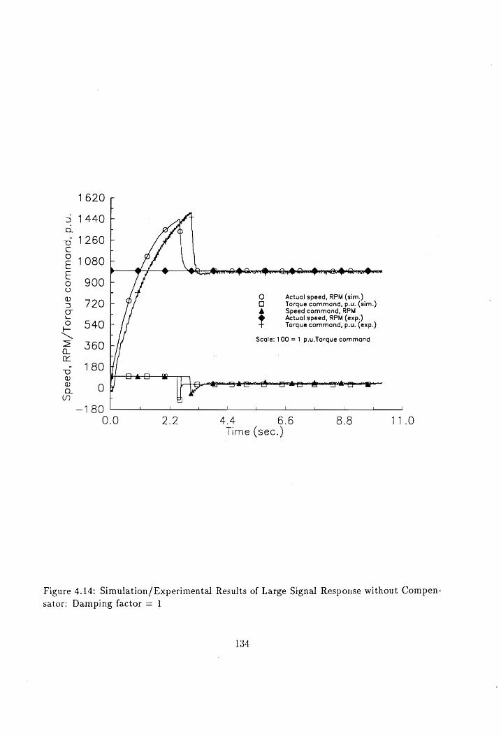
1620

3 1440 F

0 3 1260 F c L

= 1080

6 900

S720 BS Torque commend, pu aim) = @ — Aetucl speed, REM (exp.) 2 940 ? Torque command, p.u. (exp.)

> Scale: 100 = 1 p.u.Torque command = 360 oY oO 180

DT pee perth agen emlynem rg a. O §

WY L

— 80 ! | \ | ‘ | 1 | — J

0.0 2.2 4.4 6.6 8.8 11.0 Time (sec.)

Figure 4.14: Simulation/Experimental Results of Large Signal Response without Compen-

sator: Damping factor = 1

134

aT PAA

Actual speed, RPM (sim.)

oO.

540 0 Torque command, p.u. (sim.) A Speed command, ron

Actual speed, RPM (exp. 470 ? Torque command, p.u. (exp.)

Scale: 100 = 1 p.u.Torque command 300

180

60 r cheers uty de Morreraph: mm batted phe Uintah Ire L jab niece errs . yw Lt Th GU Ly Ned uo aed Ld Cy ee ud Ww

_ 60 l Le i | Le L ! Le i j

0.0 2.2 4.4 6.6 8.8 11.0 Time (sec.)

Figure 4.17: Simulation/Experimental Results of Large Signal Response with Compensator:

Damping factor = 1

139

4.6 DISCUSSION

A simple methodology has been presented in the chapter which facilitates the design of

a speed controller of the indirect vector controller controlled induction motor drive without

resorting to a computer. The algorithm has been formulated by exploiting the similarity

between the vector controlled induction motor drive and the separately excited dc motor.

The speed loop transfer function expressed in terms of T’, is significant in that it clearly

links the dynamic performance to the speed feedback and current loop time constants. It can

be observed that a faster current loop with a smaller speed filter time constant accelerates

the speed response. Expressing T in terms of the motor, converter and transducer gains

and delays using earlier expressions,

T= Th

= 1+T. (4.88)

—2(T, + Te )Tm = = + Tw

where the value of b, is given by equation 4.52. This clearly shows the influence of the

subsystem parameters on the system dynamics. A clear understanding of this would help in

the proper selection of the subsystems to obtain the required dynamic performance of the

speed controlled motor drive system. Further this derivation demonstrates that the system

behavior to a large degree depends on the subsystem parameters rather than on the current

and speed controller parameters or on the sophistication of their design.

140

Chapter 5

NOVEL SENSORLESS VECTOR CONTROL

SCHEME

5.1 INTRODUCTION

High performance inverter-fed induction motor drive systems are realized using vector

control schemes. The vector controller requires the position of the rotor flux for successful

control of the induction motor. Schemes using the measured and estimated positions of

the rotor flux are known as direct and indirect vector control schemes, respectively. The

majority of induction motor servo systems are based on the indirect vector control strategy,

which uses the machine parameters to estimate the position of the rotor flux. The modeling

of this controller and the parameter sensitivity effects are discussed in the earlier chapters.

Crucial to the success of indirect vector control is the knowledge of the rotor position which

is obtained by using position transducers.

The inclusion of a position sensor increases the cost and the mechanical complexity of

the drive system. Many applications require the minimization of the transducers in the

control strategy for reduction of cost and increased reliability of the system. Hence a novel

scheme has been proposed to eliminate the position sensor from the indirect vector control

strategy. This is achieved by modeling the induction motor in the stator reference frame

and using the airgap power. The line voltages and stator phase currents are required for

the calculation of the airgap power. While the measurement of line voltages is possible

with isolation amplifiers, it may not be a cost effective solution to low power motor drives.

Hence, the line voltages are reconstructed from the base drive signals applied to the inverter

using an algorithm proposed earlier [141]. The only input to the scheme are the two stator

141

phase currents measured by current transducers. Since the neutral of the motor is isolated,

the third phase current is obtained as the negative sum of the other two measured currents.

The base drive signals are obtained by comparing the measured and commanded values of

stator currents. The commanded values of the three phase stator currents are obtained by

the current source indirect vector control strategy.

This chapter describes the formulation and systematic derivation of the novel sensorless

vector controller scheme for induction motor drive systems. The computer simulation is per-

formed with the aid of the CAE package, VCIM, discussed in Chapter 3. The experimental

verification is performed using a DSP based vector controller, discussed in Chapter 2. The

chapter is organized as follows. The next section gives the derivation of the novel sensorless

scheme for indirect vector control induction motor drive systems. Section 5.3 presents the

simulation results obtained from the CAE package and the experimental verification is given

in Section 5.4. The various issues pertaining to this scheme and sensorless vector control

are discussed in Section 5.5.

5.2 MODELING OF THE PROPOSED SCHEME

The basic functional diagram of the proposed position sensorless vector control scheme

is presented in Fig. 5.1. Since the calculation of the airgap power is crucial to this scheme,

the modeling of the motor is performed in the stator reference frames. It can be seen

that the system consists of three modules. They are, the voltage sensing module, position

calculator module and the vector control module. The following subsections provide a

detailed description of the modeling of each of these modules.

5.2.1 Voltage Sensing Module

The voltage sensing algorithm reconstructs the line voltages from the base drive control

signals. The base drive control signals are obtained by comparing the measured stator

phase currents and the command values of the stator currents which is calculated by the

142

ac i, i ide

mains gs + . + +

+——» Rectifier V Filter VV, | Braking V Inverter supply r j de

o———__ > - . &

L

Ty...Tg Y~

Current Transform

-ation

Controller Block

d

e

al | * Ty..-16 igs lds

las Ibs les

Voltage Sensing

Transform

-ation

* Block Vas Vas lg ig

* l t T, > . Magnitude

Indirect *

Vector If Angle Positi ,

* Control Resolver osition Calculator

y o—__ > ontroler *

P Oe

Figure 5.1: Novel Position Sensorless Indirect Vector Control Scheme

143

vector control module. The inverter power circuit of the induction motor drive is shown in

Fig. 5.2. Even though transistor switches are considered, the algorithms can be suitably

modified for both thyristor and GTO switches. The following assumptions are made in the

derivation of the algorithm.

e The power transistors and freewheeling diodes are ideal switches.

e The carrier switching frequency of the inverter is limited to 2.5 kHz.

e A current source inverter is feeding the induction motor.

e The base drive signals are isolated.

A constant dc bus voltage is maintained.

A detailed description of the algorithm and the relevant equations are given in Ap-

pendix B.

5.2.2 Position Calculator Module

The position calculator module estimates the value of the rotor position from the given

set of phase voltages and currents. For a balanced three phase system, the phase voltages

obtained from the voltage sensing module can be transformed into the two axis voltages in

the stationary reference frame by,

Ugs = Vas (5.1)

1 Uds = = Vas + 2Ves 5.2

The stator currents can also be similarly transformed using the following equations,

igs = tas (5.3)

144

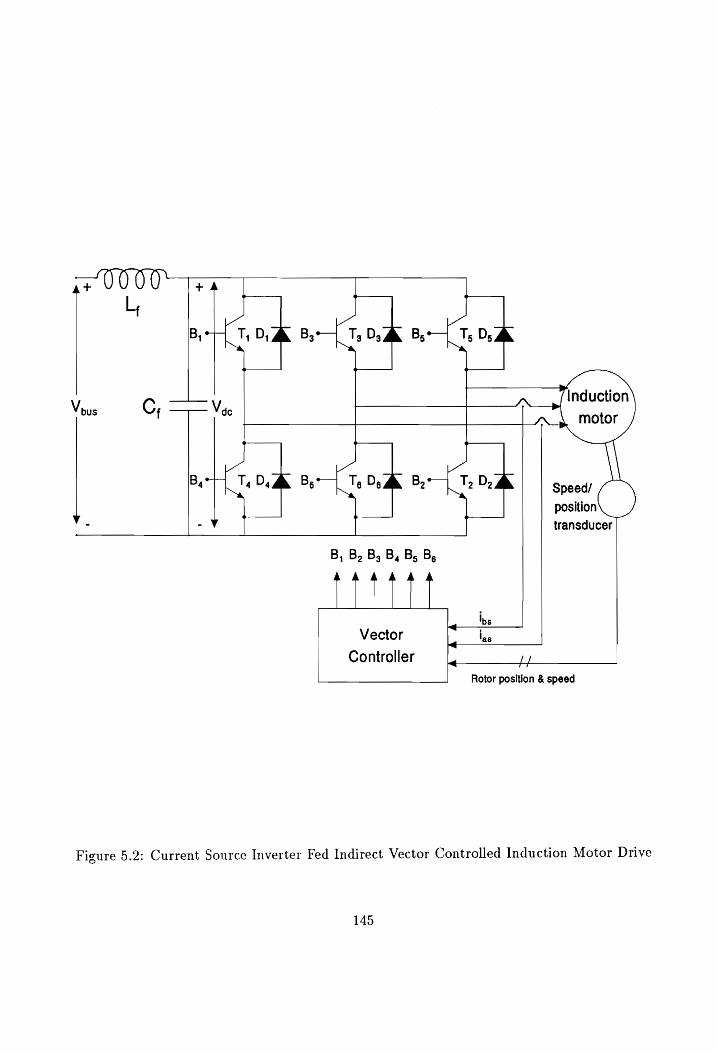
- - Vv transducer

TTT

Ing Vector las

Controller Lf Rotor position & speed

Figure 5.2: Current Source Inverter Fed Indirect Vector Controlled Induction Motor Drive

145

,; 1. ,; lds = Jae + is) (5.4)

From the phasor diagram representation of the vector controller given in Fig. 2.1, the

following relationship can be deduced.

Osc = Be + 65 + 6,

where, @,, is the stator electric angle, 6;. is the torque angle, @,; is the slip frequency

angle, 6, is the rotor position and @, is the field angle for a current source vector controller.

The dynamic equations of the induction machine in the stator reference frame is given

below.

Ugs Rs + Lsp 0 Limp 0 tgs

Vd 0 R,+L 0 Limp tds s _ s sP (5.6)

Ugr Limp —W,Lm R, + Lp —w,L, tar

Vdr Wr Lm Limp Ww, Ly R, + L,p tdr

from which the electromagnetic torque, T., is calculated using:

3 P a . Te = 9 2 Lim (tgstdr - ldstgr ) (5.7)

where, R,,R,,L;, L, are the stator and rotor resistances and self inductances, respec-

tively. ws,w, are the stator and rotor electric frequency in radians/sec. vgs, Uds, Ugr, Udr}

tgs) tds, tgry tdr are the stator and rotor, d and q axes, voltages and currents in synchronous

frames, respectively. w, is the rotor speed and the operator 4 is represented by p. The

speed is computed from the acceleration torque equation using the load torque, 7), Moment

of Inertia, J, and the viscous friction coefficient, B,

dr, Ih

P + Bu, = 5(Te- Ti) (5.8)

146

and the rotor position is given as 6, = w,t.

For the proposed scheme, only the stator phase currents and voltages are available for

computing the field angle for vector control. Since the electromagnetic torque equation

given above is dependent on the rotor currents, it cannot be used for the computation of

T. in the proposed scheme. The stator current phasor, 1,, and the stator electric angle, 6,,

are obtained from the q and d axes currents as follows,

i, = 2, + 22, (5.9)

950 = /tan7}(“32) (5.10) tds

From the dynamic model of the motor in the stator reference frame, it can be noted

that,

Ugs = (Rs + Lsp)tgs + Lin Ptgr (5.11)

Vds = (Rs + Lsp)ids + LmPtar (5.12)

Alternately, using the flux linkage model of the induction motor, the above equations

can be written as,

Uqs = Restqs + Pqs (5.13)

Uds = Rstds + Dds (5.14)

where, ws and qa, are the q and d axes stator flux linkages in the stator reference

frames. Hence the g and d axes stator flux linkages can be computed using the following

equations:

Wqs = J _ Rsiqs)dt (5.15)

147

Was = J (vs — Rsias )dt (5.16)

But, the stator d and q axes flux linkages can also be written as,

Wqs = Limtgr + Lstgs (5.17)

Wds = Lin tar + Lstds (5.18)

The rotor current equations are given as,

. vy so Lt s tqr = an (5.19)

igp = Pes = Asteds (5.20) Lm

Hence, the rotor flux linkages are given as,

War = Lintgs + Lstgr (5.21)

War = Lytds + L star (5.22)

The magnitude of the rotor flux and the field angle are then calculated using the equa-

tions,

Yr = v2, + v3, (5.23)

or War

Substituting the values of the g and d axes rotor currents in equations for the expression

6; = tan '(—) (5.24)

for electromagnetic torque,

148

(49s Pads _ tasWqs) (5.25)

(5.26)

6. = Jos (5.27)

From the phasor diagram representation of the vector controller given in Fig. 2.1, the

rotor position can be determined as,

6, = 07 — As (5.28)

Since the q and d axes stator voltages and currents, and the stator current phasors are

known, the airgap power is deduced from the following relationship,

Py = 5 (vaste + Udsias — Rei?) (5.29)

The stator frequency, w;, can be calculated from the airgap power and the electromag-

netic torque as,

P, P Ws, = — =F (5.30)

The rotor speed, w,, for closing the speed loop can then be obtained from the following

relationship,

Wr = Ws — Wel (5.31)

149

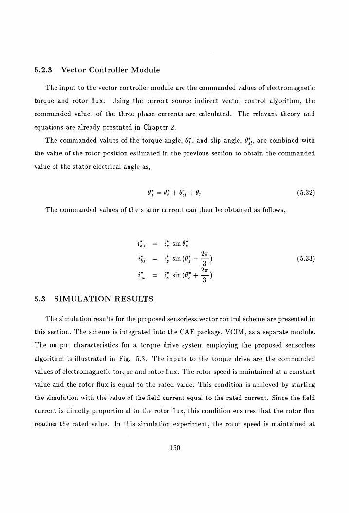
5.2.3. Vector Controller Module

The input to the vector controller module are the commanded values of electromagnetic

torque and rotor flux. Using the current source indirect vector control algorithm, the

commanded values of the three phase currents are calculated. The relevant theory and

equations are already presented in Chapter 2.

*

The commanded values of the torque angle, 07, and slip angle, 0* *;, are combined with

the value of the rotor position estimated in the previous section to obtain the commanded

value of the stator electrical angle as,

6° = 0% + 0%, +4, (5.32)

The commanded values of the stator current can then be obtained as follows,

it, = @ sing? ne ce ae OTE e= it sin(@; - =) (5.33)

2 vw, = i sin (03 + =)

5.3 SIMULATION RESULTS

The simulation results for the proposed sensorless vector control scheme are presented in

this section. The scheme is integrated into the CAE package, VCIM, as a separate module.

The output characteristics for a torque drive system employing the proposed sensorless

algorithm is illustrated in Fig. 5.3. The inputs to the torque drive are the commanded

values of electromagnetic torque and rotor flux. The rotor speed is maintained at a constant

value and the rotor flux is equal to the rated value. This condition is achieved by starting

the simulation with the value of the field current equal to the rated current. Since the field

current is directly proportional to the rotor flux, this condition ensures that the rotor flux

reaches the rated value. In this simulation experiment, the rotor speed is maintained at

150

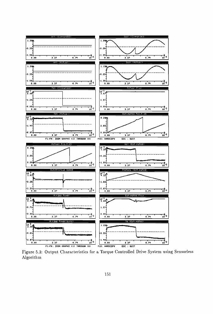
Urn (Commanded) Tasn (Commanded)

1.304 NN ——-~

ei 56 XS ei 23 » t T tT T v <-2 t T r T 2

0.00 3.37 6.79% 10 0.00 3.37 6.7% 10

CTD 1.300 i TN oN

ime ey NAY q q

Lt se > Ls 35, 5 r 1 T , t °-2 v r T v v ¥ T ' <2

0.00 3.37 €.7% 10 9.00 3.37 6.7% 10

Retyel Flue ol > io 10 §.0 3.6

Lash rrr pee etetereseres wresaceres - 157)

ré .00 T T T T T T T Tm? 0.00 T T T T T T >

0.00 3.37 ©.7% 10 2 0.00 3.37 6.7% 10 2

SEA 2 to) eT 5 | 6.2

bd 924 ~ 2.69

rs .87 t t T r ¥ Ls T T >. 0.004 T v T T T v T ™,,

0.00 3.37 6.7% 190 0.00 3.37 6.7% 10

Fi-FS: 200M GRAPHS (4) THROUGH ($¢) Fid0: HAROCOPY Esc : QUIT

—

2

6.2

68 Lo .321 |

0.00 1 )

7 T T 1 T qT t T T >, pi.50 a.m T T v + T T T vo?

0.00 3.37 6.7% 10 0.00 3.37 6.74 40

Synemronous Speed 19 3 Ta 4.0 4.2

h0.2 bL.09 ~

ri.2 F a F > PS .074 T tT i c T + v . >

0.00 3.37 6.7% 1972 0.00 3.37 6.74% 107?

ee eh ee nny TT TTT

to ¢ 10 2.7 3.6

LO. 74 1.57

r3 334 T >, 0.004 v v T T Tr v v 4 >

0.00 3.3? 6.74 1072 0.00 3.37 6.78 1072

2k 0 | 0S

hone ON ateonanienaleieansaitem Po . 324 — 4 1

2.87 T rT T T T 7 T mH ri .%8 T T T T T T T rm 0.00 3.37 6.79% 1072 0.00 3.37 6.7% 10°?

Fi-F%: ZOOM GRAPHS (1) THROUGH (%) Fi0: MAROCOPY Esc : QUIT

Figure 5.3: Output Characteristics for a Torque Controlled Drive System using Sensorless

Algorithm

0.3 p.u. which corresponds to a mechanical speed of 1080 RPM. The normalized values

of the commanded/actual speed, commanded /actual torque, commanded /actual current of

phase ‘A’, actual rotor flux and the estimated rotor position are displayed in the figure.

The inner current loop is represented by the commanded and actual values of currents.

The actual current follows the commanded value, implemented by a PWM controller with

a carrier frequency of 1 kHz. A step command of + 0.5 p.u. for the torque command and

al p.u. command for the rotor flux is applied. The actual value of the electromagnetic

torque and rotor flux closely follows the commanded signal, as seen from the figure. The

estimated value of the rotor position using the algorithm is also shown in the figure and

closely follows the actual rotor position in the system.

The output characteristics for a torque drive system for low speed operation employing

the proposed sensorless algorithm is illustrated in Fig. 5.4. In this simulation experi-

ment, the rotor speed is maintained at 0.03 p.u. which corresponds to a mechanical speed

of 108 RPM. The normalized values of the commanded/actual speed, commanded /actual

torque, commanded/actual current of phase ‘A’, actual rotor flux and the estimated rotor

position are displayed in the figure. The inner current loop is represented by the com-

manded and actual values of currents. The actual current follows the commanded value,

implemented by a PWM controller with a carrier frequency of 1 kHz. A step command of

+ 0.5 p.u. for the torque command and a 1 p.u. command for the rotor flux is applied.

It can be noted that even at this low speed the electromagnetic torque closely follows the

commanded value The rotor flux is maintained at 1 p.u. value as seen from the figure. The

estimated value of the rotor position using the algorithm is also shown in the figure and

closely follows the actual rotor position in the system.

The output characteristics for a speed drive system employing the proposed sensorless

algorithm is illustrated in Fig. 5.5. The input to the speed drive is the commanded value of

the rotor speed. This is compared with the actual value of the rotor speed. The error signal

is amplified and processed through a speed controller to get the torque command. The flux

command is obtained from the rotor speed signal by flux programming. The normalized

urn_(Conmanded)

1.024 1.0

+0 .26, 0.46

Ps .28 T 7 7 T t , ¥ t >, 0.004 T T T is 7 T T t >»

0.00 3.37 6.79 10 0.00 3.37 6.7% 10

——— 1.024 1.0

Lo 26, 0.46

ha.29 ¥ v t T t T r t >. 0 .00+ ¥ T t ¥ Oo T qt v >

0.00 3.37 6.7% 10 0.00 3.37 6.78 107?

PETER ned | : 10 10 5.0 3.6

C 4

ri .234 “ on 1.574

a 00, Ss 0.001 » t S$ t T v 7 T vv “22 T a T Tt F T t Bg 2-2

0.00 3.37 6.74 10 0.00 3.37 6.74 10

19° . 5.2¢F | 6.2

bi .36]_ ~ 2.63 7

ré .3% t oF v t F F T T an 0.004 - v T TT _— qv v T ¥ >

9.00 3.37 6.7% 10 0.00 3.37 6.7% 10°? Fi-F%: 200M GRAPHS (1) THROUGH (3) Fi0: HAROCOPY Esc : Quly

Actual Fos ition Hsl (Estimated)

Sr en

2.69. bO 324

0.004 T T a Tt T T T T >» sae T t T ~ ~ t Tt Ts

0.00 3.37 6.7% 10 0.00 3.37 6.7% 10°2

Synchronous Speed Thetash (Estimated)

io > to" tt 4.6

q j PO .674 ant

7

%

P3. 13 r 7 1 T a F T T >» rS S74 T Li v v rn v t v >

0.00 3.3? 6.7% 10 0.00 3.3? 6.74 1072

Ea Yue tL Pe Tyee ed |

10 19 — 2.2 A 3.4 ~~

ro.58 YY 1.43

r2 704 T T T T oT T t T >, 0 004— iF oT v f OE v T £

0.00 3.37 6.7% 10 6.00 3.3? 6.74 1072

Laie ke ter sale

ce eee Baer

A J

1 ro. 24.

r2. 194 T T T T r T qT T >. La T T T 1 oT v T 7 >

0.00 3.37 6.7% 10 0.00 3.37 6.7% 10°72 Fi-F%: ZOOM GRAPHS (1) THROUGH ($) Fi0: MAROCOPY Esc : UIT

Figure 5.4: Output Characteristics for a Low Speed Torque Controlled Drive System using

Sensorless Algorithm

153

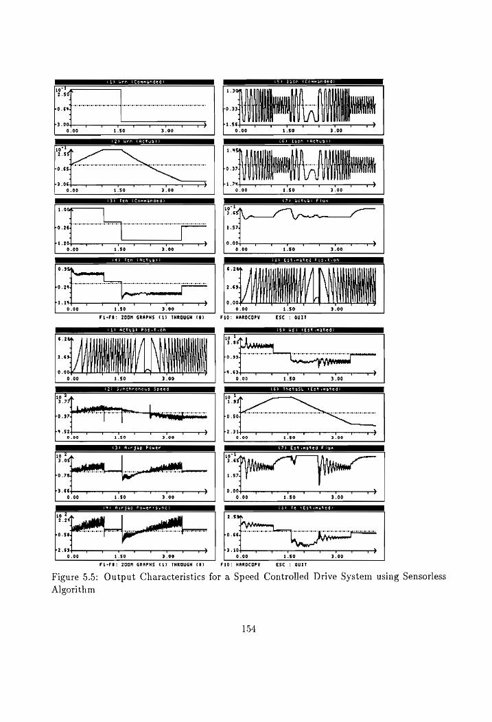
(1) urn (Commanded) (8) Tesn (Commanded)

fs —

Lo gat rrr rnp etree

r3.00 t 7 T T 7 qT t >

0.00 1.50 3.00

to" 2.8

bO.¢

L306. 5 T 1 T q t 7 T T 7 F

0.00 1.80 3.00

(7) actual Flux De ogee =

a) 19 ‘ f | 3.6

Lo.2efttstC—<CSSSCS —_ 1.57

Pi .20 T T T T T 7 T T >

0.00 1.$0 3.00

0.9%

Lo auf tr tea cstsessseserererenenerene ssn

ri. d® T TOT ¥ T t T t >

0.00 1.50 3.00

FL-FS: 200M GRAPHS (14) THROUGH (9) F10: HAROCOPY ESC : Quit

(t) AMetusl Pos.t.on

(2) Synmenmronous Speed (CO SSE Sa Et)

bs .S24 ; Ss v t T a r T TO

(7) Estimated Flux IPC 10 3.6

1.57

0.00 T T T T T T T T > 1.50 3.00

F

6.00

Co) Te (estimated)

2.50”

PO .664

P2634 T T T T T T T md L340 T T T T “T T T — 0.60 1.50 3.90 0.00 1.50 3.00

Fi-F%: ZOOM GRAPHS (%) THROUGH (?) F10: HARDCOPY esc : Quit

Figure 5.5: Output Characteristics for a Speed Controlled Drive System using Sensorless

Algorithm

154

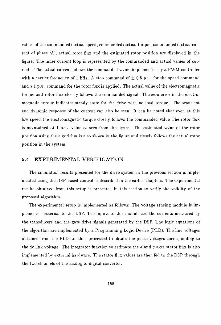
values of the commanded /actual speed, commanded/actual torque, commanded /actual cur-

rent of phase ‘A’, actual rotor flux and the estimated rotor position are displayed in the

figure. The inner current loop is represented by the commanded and actual values of cur-

rents. The actual current follows the commanded value, implemented by a PWM controller

with a carrier frequency of 1 kHz. A step command of + 0.5 p.u. for the speed command

and a1 p.u. command for the rotor flux is applied. The actual value of the electromagnetic

torque and rotor flux closely follows the commanded signal. The zero error in the electro-

magnetic torque indicates steady state for the drive with no load torque. The transient

and dynamic response of the current can also be seen. It can be noted that even at this

low speed the electromagnetic torque closely follows the commanded value The rotor flux

is maintained at 1 p.u. value as seen from the figure. The estimated value of the rotor

position using the algorithm is also shown in the figure and closely follows the actual rotor

position in the system.

5.4 EXPERIMENTAL VERIFICATION

The simulation results presented for the drive system in the previous section is imple-

mented using the DSP based controller described in the earlier chapters. The experimental

results obtained from this setup is presented in this section to verify the validity of the

proposed algorithm.

The experimental setup is implemented as follows: The voltage sensing module is im-

plemented external to the DSP. The inputs to this module are the currents measured by

the transducers and the gate drive signals generated by the DSP. The logic equations of

the algorithm are implemented by a Programming Logic Device (PLD). The line voltages

obtained from the PLD are then processed to obtain the phase voltages corresponding to

the dc link voltage. The integrator function to estimate the d and q axes stator flux is also

implemented by external hardware. The stator flux values are then fed to the DSP through

the two channels of the analog to digital converter.

155

Once the stator flux values are available in the DSP, the position estimator module

computes the rotor position using the algebraic expressions described earlier. The inverse

tangent function to compute the field angle is stored as tables and retrieved in the assembly

program. The integration function to obtain the slip angle from slip speed is implemented

by trapezoidal algorithm.

The estimated value of the rotor position is input into the vector controller algorithm

described earlier and the three phase commanded values of currents are generated. The

actual values of the current are controlled to follow the commanded values with the PWM

timers built-in the processor. The simulation results for the step torque characteristics of a

torque drive system employing the proposed sensorless algorithm is illustrated in Fig. 5.6.

The motor is allowed to accelerate to a certain speed value from standstill. The normal-

ized values of the commanded /actual speed, commanded /actual torque, commanded /actual

current of phase ‘A’, actual rotor flux and the estimated rotor position are displayed in this

figure. The inner current loop is represented by the commanded and actual values of cur-

rents. The actual current follows the commanded value, implemented by a PWM controller

with a carrier frequency of 1 kHz. A step command of torque and a 1 p.u. command for

the rotor flux is applied. It can be noted that the electromagnetic torque closely follows

the commanded value The rotor flux is maintained at 1 p.u. value as seen from the figure.

The estimated value of the rotor position using the algorithm is also shown in the figure

and closely follows the actual rotor position in the system.

The experimental validation for this condition is presented in Fig. 5.7. The commanded

value of torque and the rotor speed value in RPM is presented in this figure. Similar to the

simulation, a step command of torque is applied and the motor is started from standstill.

The position sensor is removed from the experimental setup and the estimated position is

applied to the algorithm in place of the sensor position. The response of the speed for this

condition shown in this figure closely follows the simulation results presented earlier in Fig.

5.6. The output characteristics for the speed drive can then be obtained by closing the

outer speed loop similar to that of the sensor based vector control.

156

C1) Hen (Commanded)

1.300

J ro .334

4

4 6. 5 ri.s r r > - 0.00 2.88

0.00

Peak oe

1972 3.0

4.28

0.00 T T T T ——1->

EEA ke

10

7 AAA He Seana

ba .og. 7 j mo | | |

| | | G j A

t T T r 8 .934 T T T T “T “T T > 0.00 2.88 S.75 0.00 2.88 5.75

lotta Ve | Ofg 10 19 1.9 3.6

4

0.824 1.554

0.00. > : t qT T T CF

0.90 2.88 5.75

ee hk [a-d 19 2.08F

w

T T § 75

Fi-F@: 200M GRAPHS (1) THROUGH (3)

(1) Actual Fosition

(S) Hsi (Estimated)

3.6

1.55

0.004 wT T qT o >

0.00 2.88 5.75

1 - T

0.00 2.88 5.78

C6) Thatsth t&stinsted)

wwe q v T T + 7 T vo

6.00 2.88 5.75

(3) Airgap Power

C7) Estinated Fiua

r§ 50+ ? t T T ¥ > 0.004 iF t T T v T rs F >

9.00 2.38 5.75 0.00 2.88 5.75

Ft-F@: 200M GRAPHS (1) THROUGH (2) FiO: HARDCOPY Esc : QUIT

Figure 5.6: Simulation Results of Step Torque Response using Sensorless Algorithm

157

1400 oe __. _[

Patel

TO Cc oc

£

5 © 1000 e- Actual Speed

3 5 800 C = a 600 O

® a 400- Torque Command -———————

2 200 ‘ om

6) 1 U F t t t T

0 2 4 6 8 10 12 14 16

Time, sec.

Figure 5.7: Experimental Results of Step Torque Response using Sensorless Algorithm

158

5.5 DISCUSSION

A novel sensorless vector control scheme which requires only two current transducers for

the measurement of phase currents is formulated in this chapter. The phase voltages are

estimated from the gate drive signals and the phase current measurement from which the

rotor position is obtained. The simulation results of a torque drive for different values of

rotor speed is presented to verify the algorithm. A speed drive simulation is also presented

using the sensorless algorithm to illustrate the four quadrant operation of the drive system

without position sensors.

The experimental verification has been performed by employing the DSP based vector

controller discussed in the earlier chapters. An experimental run for the torque drive system

using this setup is presented to validate the algorithm. It was noted that the switching

frequency of the PWM controller was limited to 1 kHz. due to the software limitation

of the processor. This introduced large ripples in the current which introduced errors

in the position estimator routine. Also the leakage inductance of the motor used in the

experimental setup was significant enough to introduce deviations in the estimation of the

rotor flux. These two factors has limited the implementation of the speed drive system

using the current experimental setup.

This disadvantage can be overcome by implementing the algorithm by analog circuitry

or by using a faster Digital Signal Processor to perform only the mathematical calculations.

The PWM algorithm can be made to function externally, thus enabling the user to control

the current ripple. With such a setup, the speed drive can be implemented and critical issues

such as parameter sensitivity of this algorithm and adaptation schemes can be evaluated.

159

Chapter 6

CONCLUSIONS

6.1 INTRODUCTION

With the advent of vector control and the recent advances in the semiconductor technol-

ogy, ac machines are replacing the conventional dc machines in many industrial applications.

In spite of the numerous advantages of the vector controlled induction motor drive systems,

there are certain key issues which needed to be addressed in detail. The first issue pertaining

to the classification and the modeling, simulation and analysis of the different types of vec-

tor control schemes in the popular d-q reference frames, and the parameter sensitivity and

adaptation schemes for the indirect vector controlled induction motor drive systems is given

in detail. The next issue relating to the formulation and development of a Computer Aided

Engineering package for vector controlled induction motor drive systems which includes all

the subsystem modeling in an user friendly environment is presented. The development

of an algorithm similar to the dc motor for the study and design of a speed controller is

dealt with in the next section. Finally the modeling, analysis simulation and experimental

verification of a novel sensorless vector control scheme is also presented in this dissertation.

The next section discusses the various tasks which have been accomplished and the

contributions of this research work. The final section of this chapter identifies scope for

further research in this direction.

6.2 CONTRIBUTIONS

A comprehensive literature survey was performed and the tasks to be performed in this

dissertation were identified. The author believes that the following are the contributions of

160

this work:

1. A comprehensive literature survey has been performed on vector control issues and

key issues of research identified. The modeling, simulation and analysis of the various

vector control schemes, all in the d-q reference frames, have been performed and the

results presented. To confirm the validity of the simulation results, the indirect vector

controlled induction motor drive system is implemented experimentally with a DSP

based controller.

2. The methodology for the development of a CAE package for the dynamic analysis of

the different vector control strategies which includes all the models of the various sub-

systems is developed. This package would help in the assessment of the torque ripple,

losses, efficiency, torque, speed, and position responses and their bandwidth evalua-

tion and determine the suitability for a particular application. The various results

are presented to highlight the capability and features of the CAE package. Based

on the principle of development of this package, CAE packages for other brushless

drive systems such as the permanent magnet synchronous motor, permanent magnet

brushless dc motor and the switched reluctance motor drives are also developed.

3. By utilizing the similarity between the vector controlled induction motor drive sys-

tems and the separately excited dc motor drive systems, a method for designing the

parameters for the speed controlled in a speed/position drive system is formulated

and analyzed. The results obtained from the analytical derivations are incorporated

into the CAE package and the simulation results presented and discussed. The ex-

perimental verification of the results is also performed with the DSP based vector

controller.

4. A novel sensorless vector control scheme with only current transducers is proposed

and the modeling and analysis are presented. The simulation results from the CAE

package for different conditions of the torque drive and the speed drive system are

presented to validate the proposed algorithm.

161

6.3 FUTURE RECOMMENDATIONS

Based on the work accomplished in this dissertation, the author believes that the fol-

lowing tasks are recommended for possible future work:

1. Subsystem modeling: Even though, the various subsystems in the motor drive

system has been incorporated into the CAE package, VCIM, the author believes more

detailed modeling of all the subsystems for different conditions can be accomplished

to make the package an even more efficient tool.

2. Parameter sensitivity: The various issues relating to parameter sensitivity were

discussed in the earlier chapters. The sensorless vector control scheme presented is

based on the indirect vector technique, which is itself parameter sensitive. Hence,

a detailed parameter sensitive study on this algorithm and adaptation technique to

alleviate this problem can be performed. Since the airgap power is already available

in this method, an earlier adaptation method based on airgap power calculation can

be an ideal candidate [41, 42].

162

[1]

[4]

[5]

[6]

[7]

[8]

[9]

[10]

REFERENCES

Abbondanti, A., “Method of Flux Control in Induction Motors Driven By Variable

Frequency, Variable Voltage Supplies,” Conf. Record of IEEE Industrial Applications

Society International Semiconductor Power Converter Conference, pp. 177-184, 1977.

Akagi, H., Nabae, A., “High Performance Control Strategy of Cycloconverter-Fed

Induction Motor Drive System Based on Digital Control Theory,” Trans. on IEEE-

Industrial Electronics, vol. [E-33, no. 2, pp. 126-131, May 1986.

Akagi, H., Masaki, R., Takahashi, I., Nabae, A., “Decoupled Optimum Current Con-

trol of Cycloconverter Induction Machine System,” Electrical Engineering in Japan,

vol 103, no 2, pp. 115-121, Mar/Apr 1983.

Andria, G., Dell’Aquila, A., Salvatore, L., “Signal Processing For Determining Flux

and Torque of Induction Motors,” Conf. Record of Third International Conference on

Power Electronics and Variable Speed Drives, Conf Publ. no 291, pp. 296-301, July

1988.

Andria, G., Dell’Aquila, A., Salvatore, L., “On-Line Identification of Induction Motor

Parameters,” Proc. Symposium on Electrical Drive, pp. 201-214, Sep 1987.

Ansuj, S., Shokooh, F., Schinzinger, R., “Parameter Estimation for Induction Ma-

chines Based on Sensitivity Analysis,” Trans. on IEKE-Industry Applications Society,

vol IA-25, no 6, pp. 1035-1040, Nov/Dec 1989.

Artime, J., Diez, A., Sanz, J., “A New Method for On-Line Estimation of Induction

Motor Parameters,” Proc. Third International Conference on Electrical Machines and

Drives, pp. 226-228, Nov 1987.

Baader, U., Depenbrock, M., Gierse Georg., “Direct Self-Control of Inverter-Fed In-

duction Machine Basis for Speed Control without Speed-Measurement,” Conf. Record

of IEEE-Industry Applications Society Annual Meeting, vol 1, pp. 486-492, Oct 1989.

Bassi, E., Benzi, F., Bolognani, S., Buja, G.S., “A Field Orientation for Current Fed

Induction Motor (CSIM) Drive Based on the Torque-Angle Closed Loop Control,”

Conf. Record of IEEE-Industry Applications Society Annual Meeting, vol 1, pp. 384—

389, Oct 1989.

Bassi, E., Benzi, F., “Vector Control for Induction Machine Drives : Theoretical

Aspects and Applications Examples (Italian),” Energia Elettrica, vol 63, no. 7-8, pp.

291-306, Jul-Aug 1986.

163

(11]

[12]

[13]

[14]

[15]

[16]

[17]

[18]

[19]

[20]

Bausch, H., Hontheim, H., Kolletschke, H. -D., “The Influence of Decoupling Methods

on the Dynamic Behaviour of a Field-Oriented Controlled Induction Machine,” Proc.

ICEM ’86 Munchen. International Conference on Electrical Machines, vol 2, pp. 648-

651, Sep 1986.

Bayer, K.H., Blaschke, F., “Stability Problems with the Control of Induction Motors

using the Method of Field Orientation,” Conf. Record of IFAC Symposium on Power

Electronics, pp. 483-492, 1977.

Bedingfield, R.A., “Development of CAE System for Switched Reluctance Motor

Drive Systems,” M.S. Thesis, The Bradley Department of Electrical Engineering,

Virginia Polytechnic Institute & State University, Blacksburg, VA, Jul 1991.

Bellini, A., Gifalli, G., Ulivi, G., “A Microcomputer Based Direct Field Oriented

Control of Induction Motors,” Proc. ICEM ’86 Munchen. International Conference

on Electrical Machines, vol 2, pp. 652-655, Sep 1986.

Ben-Brahim, L., Kawamura, A., “Digital Current Regulation of Field Oriented Con-

trolled Induction Motor Based on Predictive Flux Observer,” Conf. Record of IEEE-

Industry Applications Society Annual Meeting, vol 1, pp. 601-612, Oct 1990.

Benvenuto, F., Burdese, G., De Luca, S., Moroni, R., “Torque Regulation of a Con-

trolled Current Induction Motor Drive using Field Orientation Technique,” Conf.

Record of Colloque International Sur la Commande et la Regulation Numeriques des

Machines Electriques Lyon, pp. [V/58-67, Apr 1980.

Bishop, K.W.J., McLoughlin, P.D., “The Impact of Technology on Inverter Drives,”

Conf. Record of Second International Conference on Power Electronics and Variable-

Speed Drives, Conf. Publ. no 264, pp. 106-111, Nov 1986.

Bishop, K.W.J., Critchley, D.R., “Future of Inverter Fed Induction Drives,” Proc.

Conference on Drives/Motors/Controls, pp. 40-47, Oct 1983.

Biswas, S.K., Sendaula, H., Caro, T., “Self Tuning Vector Control for Induction

Motors,” Proc. IEEE Industrial Electronics Conference, pp. 276-280, Nov 1989.

Biswas, $.K., Sathiakumar, S., Vithayathil,J., “A Direct Torque Angle Controlled CSI

Fed Induction Motor Drive with Constant Slip Frequency Operation ”. Conf. Record

of IEEE-Industry Applications Society Annual Meeting, pp. 210-215, Sep 1986.

Biswas, $.K., Sathiakumar, S., Vithayathil, J., “High Efficiency Direct Torque Con-

trol Scheme for a CSI Fed Induction Motor Drive,” Conf. Record of IEEE-Industry

Applications Society Annual Meeting, pp. 216-221, Sep 1986.

Blaschke, F., “Das Verfahren der Feldorientierung zur Regelung der Drehfelima-

chine (German),” (“The Method of Field Orientation for Control of Three Phase

Machines,”) Ph.D. Dissertation, TU Braunschweig, 1973.

164

[23]

[24]

[25]

[26]

[27]

[28]

[29]

[30]

[31]

[32]

[33]

[34]

[35]

Blaschke, F., “The Principle of Field Orientation as Applied to the New Transvektor

Closed-Loop Control System for Rotating-Field Machines,” Szemens Review, vol 34,

pp. 217-220, May 1972.

Blaschke, F., “A New Method For the Structural Decoupling of AC Induction Ma-

chines,” Proc. IFAC’ Symposium, Dusseldorf, pp. 1-15(6.3.1), Oct 1971.

Blaschke, V.F., Ripperger, H., Steinkonig, H., “Regelung umrichtergespeister Asyn-

chronmaschinen mit eingepragtem Standerstrom (German),” Stemens-Zeitschrift, no.

42, pp. 773-777, 1968.

Blasko, V., Moreira, J.C., Lipo, T.A., “A New Field Oriented Controller Utilizing

Spatial Position Measurement of Rotor End Ring Current,” Conf. Record of IEEE

Power Electronics Specialists’ Conference, pp. 295-300, Jun 1989.

Boldea, I., Pfeiffer, I., Trica, A., “Modified Sliding Mode (MSM) Versus PI Speed

Control of a Current- Controlled Field-Oriented Induction Motor Drive,” Electric

Machines and Power Systems, vol 16, no. 3, pp. 209-223, 1989.

Boldea, I., Nasar, S.A., “Torque Vector Control (TVC) - A Class of Fast and Robust Torque - Speed and Position Digital Controllers for Electric Drives,” Electric Machines

and Power Systems, vol 15, no. 3, pp. 135-147, 1988.

Brostov, Y.A., Pashkov, N.N., Junger, I.B., “Induction Zero Overshoot Response

Nonlinear Model Control,” Electric Technology U.S.S.R., no 2, pp. 35-41, 1987.

Bose, B.K., “Sliding Model Control of Induction Motor,” Conf. Record of IEEE-

Industry Applications Society Annual Meeting, pp. 479-486, Oct 1985.

Bose, B.K., “Scalar Decoupled Control Induction Motor,” Trans. on IEEE-Industry

Applications Society, vol [A-20, no 1, pp. 216-225, Jan/Feb 1984.

Brickwedde, A., “Cycloconverter Fed High Performance Induction Motors for Rolling

Steel Mill Industrial Drives,” Proc. Second European Conference on Power Electronics

and Applications, vol 2, pp. 1181-1189, Sep 1987.

Cahill, T.M., “Microprocessor Based Vector Controlled Induction Spindle Drive -

Application Considerations,” Proc. Sizth Annual Control Engineering Conference,

pp. 50-54, May 1987.

Cardwell, B.J., “Torque Control of AC Induction Motor Traction Drives,” Conf.

Record of International Conference on ‘Electric Railway Systems for a New Century’,

(Conf. Publ. no 279), pp. 73-77, Sep 1987.

Chan, C.C., Wang, H., “An Effective Method for Rotor Resistance Identification for

High- Performance Induction Motor Vector Control,” [FEE Transactions on Indus-

trial Electronics, vol 37, no. 6, pp. 477-482, Dec 1990.

165

[36]

[37]

[38]

[42]

[43]

[44]

[45]

[46]

[47]

Cheng-lin, Gu., Xing-shi, T., “A Microprocessor Based PWM Variable-Speed System

with Modified Field Oriented Control,” Proc. ICEM ’86 Munchen. International

Conference on Electrical Machines, vol 2, pp. 660-663, Sep 1986.

Chura, V., “Squirrel-Cage Motor Controlled Stator Leakage Flux,” Acta Tech. CSAV

(Czechoslovakia), vol 30, no 4, pp. 117-125, 1985.

Colleran, P.J., Rogers, W.E., “Controlled Starting of AC Induction Motors,” Trans.

on IEEE Industry Applications Society, vol IA-19, no. 6, pp. 1014-1018, Nov/Dec

1983.

Critchley, D.R., Jones, R., “High Performance AC Controller,” [EE Colloquium on

‘Control of Induction Motors’, (Digest no 60), pp. 5/1-3, Apr 1989.

Daboussi, Z., Mohan, N., “Digital Simulation of Field-Oriented Control of Induction

Motor Drives Using EMTP,” Trans. on IEEE Energy Conversion, vol 3, no 3, pp.

667-673, Sep 1988.

Dalal, D., Krishnan, R., “Parameter Compensation for Indirect Vector Controlled

Induction Motor Drive using Estimated airgap power,” Conf. Record of IEE E-Industry Applications Society Annual Meeting, pp. 170-176, Oct 1987.

Dalal, D., “Novel Parameter Compensation Scheme for Indirect Vector Controlled

Induction Motor Drives,” M.S. Thesis, The Bradley Department of Electrical Engi-

neering, Virginia Polytechnic Institute & State University, Blacksburg, VA, Jul 1987.

Debowski, A., “Indirect Control Based on Dual Observer for Current-Fed Induction

Motor by Field Weakening,” Proc. Symposium on Electrical Drive, pp. 201-214, Sep

1987.

Debowski, A., “Indirect Field Oriented Control for Current-Fed Induction Motor

Based on Dual Observer,” Proc. ICEM ’86 Munchen. International Conference on

Electrical Machines, vol 2, pp. 860-863, Sep 1986.

De Doncker, R.W., Profumo, F., Pastorelli, M., “Self Tuning of Induction Motor Servo

Drives using the Universal Field Oriented Controller,” Proc. IEEE Power Electronics

Specialists’ Conference, pp. 649-655, Jun 1990.

De Doncker, R., Profumo, F., “The Universal Field Oriented Controller Applied to

Tapped Stator Windings Induction Motors,” Conf. Record of IEEE Power Electronics

Specialists’ Conference, pp. 1031-1036, Jun 1989.

De Doncker, R.W., Novotny, D.W., “Universal Field Oriented Controller,” Conf.

Record of IEEE Industry Applications Society Annual Meeting, pp. 450-456, Oct 1988.

166

[48]

[49]

(50)

[51]

[52]

[53]

[54]

[57]

[58]

De Doncker, R., “Field Oriented Controllers with Rotor Deep Bar Compensation

Circuits,” Conf. Record of IEEE Industry Applications Society Annual Meeting, pp.

142-149, Oct 1987.

De Doncker, R., Vandenput, A., Geysen, W., “Thermal Models of Inverter Fed Asyn-

chronous Machines Suited for Adaptive Temperature Compensation of Field Oriented

Controllers,” Conf. Record of IFEE Industry Applications Society Annual Meeting,

pp. 132-139, Sep 1986.

De Doncker, R.W., Vandenput, A., Geysen, W., “A Digital Field Oriented Con-

troller Using the Double Cage Induction Motor Model,” Conf. Record of IEEE Power

Electronics Specialists’ Conference, pp. 502-509, Jun 1986.

Delfiore, S., Franceschini, G., Tassoni, C., “Spice Aided Analysis of UPS Vector Con-

trol,” Proc. Eleventh International Telecommunications Energy Conference - Intelec

89. Part 2 (of 2), Oct 1989.

Del Pizzo, A., Pagano, E., Perfetto, A., “Comparative Analysis and Parameter Sen-

sitivity of Field Oriented Speed Controlled Asynchronous Motors,” Proc. Fourth

International Conference on Electrical Machines and Drives, pp. 322-327, Sep 1989.

Denoncin, A.L., Charleroi, B., “Experience ACEC/MIVA,” Proc. Power Electronics

and Applications, vol 2, pp. 5/89-93, Oct 1985.

Denoncin, L., Detemmerman, B., Lataire, P., “Control of a Current Inverter-Fed

Asynchronous Machine for Railway Traction and Alternative Motors in General,”

Conf. Record of Control in Power Electronics and Electrical Drives, pp. 643-650, Sep

1984.

Depenbrock, M., “Direct Self-Control (DSC) of Inverter-Fed Induction Machine,” Trans. on IEEE-Power Electronics, vol 3, no 4, pp. 420-429, Oct 1988.

Diana, G., Harley, R.G., “Aid for Teaching Field Oriented Control Applied to Induc-

tion Machines,” IEEE Transactions on Power Systems, vol 4, no. 3, pp. 1258-1262,

Aug 1989.

Diez, A., Garcia, D.F., Cancelas, J.A., Lopez, H., “Adaptive Control of an Asyn-

chronous Eolic Generator using the Field-Oriented Technique,” Mediterranean Elec- trotechnical Conference (MELECON 789), pp. 99-104, Apr 1989.

Dimitri, D.S., Olson, W., Berg, D., “A.C. Induction Motor - Vector Control Cubic

Motion Generator Dispenses Glue in Smooth, Continuous flow over Irregular Shapes,”

IEEE Conf. Record of Fortieth Annual Conference of Electrical Engineering Problems

in Rubber and Plastic Industries, pp. 52-59, April 1988.

167

[59] Eisenbrown, R., Kerkkanen, Y., “High Performance AC Drives for Pulp and Paper Mill Application,” Conf. Record of IFEE-Annual Pulp and Paper Industry Technical

Conference, pp. 177-187, Jun 1984.

[60] Erdman, W.L., Hoft, R.G., “A Trajectory Sensitivity Approach to Parameter Distur- bance Problems in Indirect Field Oriented Drive Systems,” Conf. Record of IEEE-

Industry Applications Society Annual Meeting, pp. 617-631, Oct 1989.

[61] Finch, J.W., Acarnley, P.P., Atkinson, D.J., “Practical Lnplementation and Test

Facility for Field Oriented Induction Motor Drives,” Proc. Fourth International Con-

ference on Electrical Machines and Drives, pp. 288-292, Sep 1989.

(62] Floter, W., Ripperger, H., “Field-Oriented Closed-Loop Control of an Induction

Machine with Transvektor Control System,” Siemens Review, vol 39, no 6, pp. 248-

252, Jun 1972.

[63] Floter, W., Ripperger, H., “Field Oriented Closed-Loop Control of an Induction

Machine with the New TRANSVECTOR Control System,” Stemens-Z.45, pp. 761-

764, 1971.

[64] Fratta, A., Vagati, A., Villata, F., “Vector Control of Induction Motors without Shaft

Transducers,” Conf. Record of IEEE-Power Electronics Specialists’ Conference, vol

2, pp. 839-846, Apr 1988.

[65] Fujisawa, T., Akita, k., “Sampling Time Effects on the Slip-Frequency-Type Vector

Control of an Induction Motor,” Electrical Engineering in Japan ( English translation

of Denki Gakkkai Ronbunshi), vol 109, no. 5, pp. 85-92, Sep-Oct 1989.

[66] Fulton, D.E., “Characteristics of Induction Servos,” Proc. Ninth International Motor Con Conference, pp. 109-115, Oct 1986.

[67] Fulton, D.E., “Poor man’s Vector Control or a User’s Guide to Introduction Motor

Servos,” Proceedings of the Fifth Annual Control Engineering Conference, pp. 391-

397, May 1986.

(68] Gabriel, R., Leonhard, W., “Microprocessor Control of Induction Motor,” Proc.

International Semiconductor Power Converter Conference, pp. 385-396, May 1982.

[69] Gabriel, R., Leonhard, W., Nordby, C., “Field Oriented Control of a Standard AC- Motor Using Microprocessor,” Trans. on IEEE-Industry Applications Society, vol

IA-16, no 2, pp. 186-192, Mar/Apr 1980.

[70] Gabriel, R., Leonhard, W., Nordby, C., “Microprocessor Control of Induction Mo-

tors Using Field Coordinates,” Proc. IEEE International Conference on Electrical

Variable-Speed Drives, pp. 146-150, Sep 1979.

168

[71] Galler, D., “Energy Efficient Control of AC Induction Motor Driven Vehicles,” Conf.

Record of IEEE Industry Applications Society Annual Meeting, pp. 301-308, Oct 1980.

[72] Garces, L.J., “Parameter Adaptation for Speed Controlled Static AC Drive with Squirrel Cage Induction Motor,” Conf. Record of IFEE-Industry Applications Society

Annual Meeting, pp. 843-850, Oct 1979.

[73] Garcia-Cerrada, A., Taufiq, J.A., “Convergence of Rotor Flux Estimation in Field

Oriented Control,” Conf. Record of Third International Conference Power Electronics

and Variable Speed Drives, (Conf. Publ. no 291), pp. 291-295, July 1988.

[74] George, N.R., “Speed Control of DL Motor Using Triac Electronic Regulator for Supply and Winder Drives in Cable Industry,” Electric India (India), vol 26, no 16,

pp. 5-10, Aug 1986.

[75] Gerasimyak, R.P., “Frequency Characteristics of an Induction Motor with Parametric

Control of the Stator and Rotor Circuits,” Elektrotekhnika (USSR), vol 56, no 11, pp. 31-34, 1985.

[76] Gol, O., “Modelling of Inverter/Induction-Machine Drives,” Conf. Record of Inter-

national Conference on Electrical Machines, vol 2, pp. 670-677, Sep 1980.

[77] Gratzfeld, P., Weinhardt, M., “Improvement of the Dynamic Behavior of a Bogie

Drive with Two Induction Motors Fed by a Common Inverter ,” Conf. Record of

International Power Electronics Conference, vol 2, pp. 1556-1566, Mar 1983.

[78] Grieve, D.W., Cross, D.M., “Recent Developments in the Design and Applications of

Large, High Performance Cycloconverter Drive Systems,” Conf. Record of Third In-

ternational Conference on Power Electronics and Variable-Speed Drives, (Conf. Publ.

no 291), pp. 309-314, July 1988.

[79] Gross, D.M., Taylor, D.M., “Squirrel cage Induction Motor Cyclo-converter drive at the British Coal Wearmouth Colliery,” GEC Review, vol 4, no 3, pp. 154-163, 1988.

[80] Habtler, T.G., Divan, D.M., “Control Strategies for Direct Torque Control Using Discrete Pulse Modulation,” Conf. Record of IEEE-Industry Applications Society

Annual Meeting, vol 1, pp. 514-522, Oct 1989.

[81] Hajdu, E., Jardan, R.K., “Voltage Source Inverter Drive with Direct Torque Control,”

Conf. Record of Second International Conference on Power Electronics and Variable-

Speed Drives, (Conf. Publ. no 264) pp. 80-84, Nov 1986.

(82] Hakata, H., Yamakoshi, H., Tatara, S., “Recent Developments and Applications of AC Variable-Speed Drives for Rolling Mill Main Stands,” Toshiba Review (International

Edition), no 160, pp. 7-12, Summer 1987.

169

[83]

[84]

[85]

[87]

[88]

[89]

[90]

[91]

[92]

[93]

Halasz, $., El-Sayed, M.M., “A.C. Inverter Drive with Field Oriented Control and

Optimum PWM Strategy,” Lectures presented at the International Seminar on Mi-

croprocessors, vol 32, no. 1, pp. 67-75, Oct 1986.

Halasz, S., Schmidt, I., Horvath, M., “Transistorized PWM Inverter Asynchronous

Motor Drive,” Conf. Record of International Conference on Electrical Machines, vol

2, pp. 688-694, Sep 1980.

Harashima, F., Kondo, S., Hachiken, E., Onno, Y., Ohnishi, K., “Synchronous Watt

Torque Feedback Control of Induction Motor Drives,” Conf. Record of IFEE-Industry

Applications Society Annual Meeting, pp. 156-162, Oct 1987.

Harashima, F., Arihara, E., Ohnishi, K., Kondo, $., “Microcomputer-Controlled

Induction Motor Considering the Effects of Secondary Resistance Variation,” Conf.

Record of IEEE-Industry Applications Society Annual Meeting, pp. 548-553, Oct 1985.

Harashima, F., Kondo, S., Ohnishi, K., Kajita, M., “Multimicroprocessor-Based

Control System for Quick Response Induction Motor Drive,” Trans. on IEEE Industry

Applications Society, vol [A-21, no 3, pp. 602-609, May/Jun 1985.

Hasegawa, T., Kurosawa, R., Hosoda, H., Abe, K., “Microcomputer-Based Motor

Drive System with Simulator Following Control,” Proc. IEEE Industrial Electronics

Conference, pp. 41-46, Sep 1986.

Hashimoto, H., Ohno, Y., Kondo, S., Harashima, F., “Torque Control of Induction

Motor Using Predictive Observer,” Conf. Record of IEEE Power Electronics Special-

ists’ Conference, pp. 271-278, Jun 1989.

Hasse, K., “Zur Dynamik Drehzahlgeregelter Antriebe mit Stomrichtergespeisten

Asynchron-Kurzchlusslaufermachinen (German),”(“On the Dynamics of Speed Con- trol of Static Ac Drives with Squirrel-Cage Induction Machines,”) Ph.D. Dissertation,

TH Darmstadt, 1969.

Hirose, K., Kawamura, A., Hoft, R., “Comparison of Field Oriented and Field Acceler-

ation Methods of Induction Motor Control,” Conf. Record of IEEE-Power Electronics

Specialists’ Conference, pp. 170-180, Jun 1984.

Ho. E., Sen, P.C., “High Performance Parameter Insensitive Drive using a Series-

Connected Wound Rotor Induction Motor,” Conf. Record of 1988 IEEE Industry

Applications Society Annual Meeting, pp. 239-245, Oct 1988.

Ho, E.Y., Sen, P.C., “Digital Simulation of PWM Induction Motor Drives for Tran-

sient and Steady State Performance,” Trans. on IEEE-Industrial Electronics, vol

IE-33, no 1, pp. 66-77, Feb 1986.

170

[94]

[95]

[101]

[102]

[103]

[104]

Holtz, J., Khambadkone, A., “Vector Controlled Induction Drive with a Self-

Commissioning Scheme,” Proc. IEEE Industrial Electronics Conference, vol II, pp.

927-932, Nov 1990.

Holtz, J.. Thimm, T., “Identification of the Machine Parameters in a Vector Con-

trolled Induction Motor Drive System,” Conf. Record of IEEE-Industry Applications

Society Annual Meeting, vol 1, pp. 601-606, Oct 1989.

Holtz, J., Bube, E., “Field-Oriented Asynchronous Pulsewidth Modulation for High

Performance AC Machine Drives Operating at Low Switching Frequency,” Conf.

Record of IEEE Industry Applications Society Annual Meeting, pp. 412-417, Oct 1988.

Hombu, M., Ueda, A., Nakazato, M., “Current Source Inverters with Sinusoidal

Inputs and Outputs,” Hitachi Review, vol 36, no 1, pp. 29-34, Feb 1987.

Hori, Y., Cotter, V., Kaya, Y., “A Novel Induction Machine Flux Observer and

its Application to a High Performance AC Drive System,” Proc. Automatic Control

- World Congress, Selected Papers from the 10th Triennial World Congress of the

International Federation of Automatic Control, vol 3, pp. 363-368, Jul 1987.

Horstmann, D., Stanke, G., “Field Oriented Control with Suboriented Pulse Pattern

Generation of PWM Converter Fed Induction Machines,” 5th IFAC/IFIP Symposium

of Software for Computer Control 1988 (SOCOCO ’88), pp. 91-98, Apr 1988.

Hosoda, H., Tatara, $., Kurosawa, R., Hakata, H., Katsuhiko Doi., “New Concept

High-Performance Large-Scale AC Drive System - Cross Current type Cycloconverter

Fed Induction Motor with High-Performance Digital Vector Control,” Conf. Record

of IEEE-Industry Applications Society Annual Meeting, pp. 229-234, Sep 1986.

Hung, K.T., Lorenz, R.D., “A Stator Flux Error-Based, Adaptive Tuning Approach for Feedforward Field Oriented Induction Machine Drives,” Conf. Record of IEFEE-

Industry Applications Society Annual Meeting, vol 1, pp. 589-594, Oct 1990.

Hunter, G.P., Ramsden, V.S., “New Improved Modulation Method for a Cyclocon-

verter Driving an Induction Motor,” Proc. B IEE Electric Power Applications, vol

135, no 6, pp. 324-333, Nov 1988.

Irisa, T., Takata, S., Ueda, R., Sonoda, T., “Effect of Machine Structure on Identifi-

cation of Spatial Position and its Magnitude of Rotor Flux in Induction Motor Vector

Control,” JEE International Conference on Power Electronics and Variable-Speed

Drives, no 234, pp. 352-356, May 1984.

Irisa, T., Takata, S., Ueda, R., Sonoda, T., Mochizuki, T., “A Novel Approach on

Parameter Self Tuning Method in Ac Servo Systems,” Proc. Third IFAC Symposium

wn Power Electronics and Drives, pp. 41-48, 1983.

171

[105]

[106]

[107]

[108]

[109]

[110]

[111]

[112]

[113]

[114]

[115]

Ishida, M., Iwata, K., “Steady-State Characteristics of a Torque and Speed Control

System of an Induction Motor Utilizing Rotor Slot Harmonics for Slip Frequency

Sensing,” Trans. on IEEE Power Electronics, vol PE-2, no 3, pp. 257-263, July 1987.

Ishida, M., Iwata, K., “Steady-State Characteristics of a Torque and Speed Control

System of an Induction Motor Utilizing Rotor Slot Harmonics for Slip Frequency

Sensing,” Conf. Record of IFEE Power Electronics Specialists’ Conference, pp. 653-

660, Jun 1985.

Ishihara, K., Katayama, S., Kokubu, T., Yasaka, M., Kurosawa, R., “Application of

a New Drive Systems for Plate Mill Drives,” Trans. on IEEE-Industry Applications

Society, vol IA-22, no 2, pp. 345-351, Mar/Apr 1986.

Islam, 5.M., Somuah, C.B., “Efficient High Performance Voltage Decoupled Induction

Motor Drive with Excitation Control,” [EEE transactions on Energy Conversion, vol

4, no. 1, pp. 109-117, Mar 1989.

Iwasaki, M., Oyama, K., Tsunehiro, Y., “Current-Fed Inverter with Static Var Gen-

erator for Induction Motor Drive,” Electrical Engineering in Japan, vol 103, no 3, pp.

100-108, May/Jun 1983.

Jardan, R.K., Horvath, M., “Low Frequency Operation of Current-Fed Induction

Motors,” Proc. International Conference on Electrical Machines, vol 3, pp. 843-846,

Sep 1984.

Jardan, R.K., Horvath, M., “Current-Source Inverter Induction Motor Drive with

Field-Oriented Control,” Proc. Second Annual International Motor-Con Conference,

pp. 72-85, Mar 1982.

Jardan, R.K., Horvath, M., “Flux Control in Current Source Inverter Drives,” Conf.

Record of International Conference on Electrical Machines, vol 2, pp. 785-792, Sep

1980.

Joetten, R., Maeder, G., “Control Methods for Good Dynamic Performance Induction

Motor Drives Based on Current and Voltages as Measured Quantities,” Trans. on

IEEE Industry Applications Society, vol 1A-19, no 3, pp. 356-363, May/Jun 1983.

Kanekal, R., “Modeling, Simulation and Analysis of an Indirect Vector Controlled

Induction Motor Drive,” M.S. Thesis, The Bradley Department of Electrical En-

gineering, Virginia Polytechnic Institute & State University, Blacksburg, VA, Nov

1987. L Q g t es ‘J %, ge a an 1 S “ey

Karybakas, C.A., “Generalized Torque Performance of Two-Phase Induction Motors

Controlled By Triac-An Approximate Analysis,” Trans. on IEEE Industrial Electron-

ics and Control Instrumentation, vol IECI-28, no 1, pp. 40-45, Feb 1981.

172

[116]

[117]

[118]

[119]

[120]

[121]

[122]

[123]

[124]

[125]

[126]

Katta, T., Ibamoto, M., Narita, H., Kiwaki, H., Onoda, Y., Okamatsu, S., Tsuboi,

T., Schimuzu, Y., “High Reliability Control Circuit of PWM Inverter for Electric Car

Drive,” Conf. Record of IEEE Power Electronics Specialists’ Conference, pp. 311-317,

Jun 1979.

Kawamura, A., Hoft, R., “An Analysis of Induction Motor Field Oriented or Vector

Control,” Conf. Record of IEEE-Power Electronics Specialists’ Conference, pp. 91—

101, Jun 1983.

Kazmierkowski, M.P., Sulkowski, W., “A Novel Vector Control Scheme for Transistor

PWM Inverter-Fed Induction Motor Drive,” Trans. on IEEE-Industrial Electronics,

vol. IE-38, no. 1, pp. 41-48, May 1991.

Kazmierkowski, M.P., Sulkowski, W., “Transistor Inverter-Fed Induction Motor Drive

with Vector Control System,” Conf. Record of IEEE-Industry Applications Society

Annual Meeting, pp. 162-168, Sep 1986.

Kazmierkowski, M.P., Kopcke, H.-J., “Current Source Inverter-Fed Induction Motor

Drive System Controlled without a Speed Sensor,” Proc. Power Electronics and

Applications, vol 2, pp. 3/345-350, Oct 1985.

Kazmierkowski, M.P., Kopcke, H.-J., “A Simple Control System for Current Source

Inverter-Fed Induction Motor Drives,” Trans. on IEEE Industry Applications Society,

vol [A-21, no 3, pp. 617-623, May/Jun 1985.

Kazmierkowski, M.P., Kopcke, H.-J., “Comparison of Dynamic Behavior of Frequency

Converter Fed Induction Machine Drives,” Conf. Record of Control in Power Elec-

tronics and Electrical Drives, pp. 313-320, Sep 1984.

Kerkman, R.J., Rowan, T.M., Leggate, D., “Indirect Field Oriented Control of an

Induction Motor in the Field Weakening Region,” Conf. Record of IEEE-Industry

Applications Society Annual Meeting, vol 1, pp. 375-383, Oct 1989.

Khater, F., Lorenz, R.D., Novotny, D.W., Tang, K., “The Selection of Flux Level in

Field Oriented Induction Machine Controllers with Consideration of Magnetic Sat-

uration Effects,” JEEE transactions on Industry Applications, vol [A-23, no. 2, pp.

276-282, Mar/Apr 1987.

Kilicaslan, B., Ersak, A., “Analysis of a PWM Inverter Driven Induction Machine,”

Conf. Record of International Conference on Electrical Machines, vol 2, pp. 678-687,

Sep 1980.

Kimoto, K., Kameko, Y., Hashimoto, K., Ohnishi, “Decoupling Control of an Induc-

tion Motor Operated with a PAM Inverter,” Conf. Record of IFEE Power Electronics

Specialists’ Conference, pp. 1091-1098, Apr 1988.

173

[127]

[128]

[129]

[130]

(131]

[132]

[133]

[134]

[135]

[136]

[137]

Kirschen, D.S., Novotny, D.W., Lipo, T.A., “Optimal Efficiency Control of an Induc-

tion Motor Drive,” Trans. on IEEE-Energy Conversion, vol EC-2, no 1, pp. 70-76,

Mar 1987.

Kobayashi, T., Sahashi, M., Inomata, K., Domon, T., Suzuki, I., “Development of

an Amorphous Torque Sensor for Induction Motors,” [FEE Translation Journal on

Magnetics in Japan, Vol TMJ-2, no 12, pp 1162-1163, Nov 1985.

Kohata, M., Hayashi, H., “Quick Response Control of Induction Motor using Voltage

Source Inverter,” Conf. Record of International Power Electronics Conference, vol 1,

pp. 708-719, Mar 1983.

Kohlmeier, H., Niermeyer, O., Schroder, D., “High Dynamic Four-Quadrant AC-

Motor Drive with Improved Power Factor and on-line Optimized Pulse Pattern with

PROMC (Precalculation of Reference for Optimal Model Control),” Proc. of Power

Electronics and Applications, vol 2, pp. 3/173-178, Oct 1985.

Koyama, M., Yano, M., Kamiyama, I., Yano, $., “Microprocessor-Based Vector Con-

trol System for Induction Motor Drives with Rotor Time Constant Identification

Function,” Trans. on [IEEE-Industry Applications Society, vol IE-33, no 2, pp. 453-

459, May/Jun 1986.

Koyama, M., Sugimoto, H., Mimura, M., Kawasaki, K., “Effects of Parameter Change

on Coordinate Control System of Induction Motor,” Conf. Record of International

Power Electronics Conference, pp. 684-695, Mar 1983.

Krishnan, R. “Electronic Control of Machines,” Prentice Hall, Englewood Cliffs, NJ,

1992.

Krishnan, R., Bharadwaj, A.S., “Computer Simulation of Modern Variable Speed Motor Drive Systems,” Project Report, Submitted to Center of Innovative Technology,

VA, Jan 1992.

Krishnan, R., Bharadwaj, A.S., “A Review of Parameter Sensitivity and Adaptation

in Indirect Vector Controlled Induction Motor Drive Systems,” JE EE Trans. on Power

Electronics, vol 6, no 4, pp. 695-703, Oct 1991.

Krishnan, R., Bharadwaj, A.S., Bedingfield, R.A., “Computer Aided Simulation for

the Dynamic Analysis of the Indirect Vector Controlled Induction Motor Drive Sys-

tems,” Proc. Fifth IFAC/IMACS Symposium on Computer Aided Design in Control

Systems, pp. 583-588, University of Wales, Swansea, UK, Jul 1991.

Krishnan, R., Bedingfield, R.A., Bharadwaj, A.S., Ramakrishna P., “Design

and Development of a User-Friendly PC-Based CAE Software for the Analysis of

174

[138]

[139]

[140]

[141]

[142]

[143]

[144]

[145]

[146]

[147]

[148]

Torque/Speed/Position Controlled PM Brushless DC Motor Drive System Dynam- ics,” Conf. Record of [IEEE-Industry Applications Society Annual Meeting, pp. 1388-

1394, Oct 1991.

Krishnan, R., Bharadwaj, A.S., “Single Chip Microcontroller Implementation of an

Indirect Vector Controlled Induction Motor Drive System,” Conf. Record of IEEE

Power Electronics Specialists’ Conference, pp. 265-270, Jun 1989.

Krishnan, R. “Accuracy Response and Reliability of the Ac and Dc Motor Drive,”

Proc. Workshop on Electrical Machines and Drive, National Science Foundation

Large-Scale Nonlinear Systems Program, pp. 32-52, Oct 1988.

Krishnan, R., Pillay, P., “Parameter Sensitivity in Vector Controlled AC Motor

Drives,” Proc. [IEEE-Industrial Electronics Conference, vol 1, pp. 212-218, Nov 1987.

Krishnan, R., Doran, F.C., “A Method of Sensing Line Voltages for Parameter Adap-

tation of Inverter Fed Induction Motor Servo Drives,” Trans. on [EEE-Industry

Applications Society, vol IA-23, no 4, pp. 617-622, Jul/Aug 1987.

Krishnan, R., Doran, F.C., Lotas, T.S., “Identification of Thermally Safe Load Cycles

for an Induction Position Servo,” Trans. on IEEE Industry Applications Society, vol

IA-23, no 4, pp. 636-643, Jul/Aug 1987.

Krishnan, R., Doran, F.C., “Study of Parameter Sensitivity in High Performance

Inverter-Fed Induction Motor Drive Systems,” Trans. on IEEE Industry Applications

Society, vol [A-23, no 4, pp. 623-635, Jul/Aug 1987.

Krishnan, R., Pillay, P., “Sensitivity Analysis and Comparison of Parameter Com-

pensation Schemes in Vector Controlled Induction Motor Drives,” Conf. Record of

IEEE-Industry Applications Society Annual Meeting, pp. 155-161, Sep 1986.

Krishnan, R., Lindsay, J.F., Stefanovic, V.R., “Comparison of Control Schemes for

Inverter Fed Induction Motor Drives,” Conf. Record of IEE Conference on Power

Electronics and Variable Speed Drives, (Conf. Publ. no 234), pp. 312-316, May 1984.

Krishnan, R., “Control and Dynamics of Inverter-Fed Induction Motor,” Ph.D.

Dissertation, Concordia University, Montreal, Quebec, Canada, Mar 1982.

Krishnan, R., Stefanovic, V.R., Lindsay, J.F., “Control Characteristics of Inverter-

Fed Induction Motor,” Conf. Record of IEEE-Industry Applications Society Annual

Meeting, pp. 548-561, Oct 1981.

Krishnan, R., Maslowski, W.A., Stefanovic, V.R., “Control Principles in Current

Source Induction Motor Drives,” Conf. Record of IEEE-Industry Applications Society

Annual Meeting, pp. 605-617, Oct 1980.

175

[149]

[150]

[151]

[152]

[153]

[154]

[155]

[156]

[157]

[158]

[159]

[160]

Kubo, K., Watanabe, M., Ohmae, T., Kamiyama, K., “Fully Digitialized Speed

Regulator using Multiprocessor System for Induction Motor Drives,” Trans. on IEEE-

Industry Applications Society, vol [A-21, no 4, pp. 1001-1008, Jul/Aug 1985.

Kubota, H., Matsuse, K., Nakano, T., “New Adaptive Flux Observer of Induction

Motor for Wide Speed Range Motor Drives,” Proc. IEEE Industrial Electronics Con-

ference, vol II, pp. 921-926, Nov 1990.

Kubota, H., Matsuse, K., Fukao, T., “Indirect Field Oriented Control of CSI-Fed

Induction motor with State Observer,” Conf. Record of IEEE Industry Applications

Society Annual Meeting, pp. 138-141, Oct 1987.

Kubota, H., Matsuse, K., Fukao, T., “New Control] Method of Inverter-Fed Induction

Motor Drive by using State Observer with Rotor Resistance Identification,” Conf.

Record of IEEE-Industry Applications Society Annual Meeting, pp. 601-606, Oct 1985.

Kubota, H., Matsuse, K., Fukao, T., “A Control Method of Induction Motor Driven

by Current-Source Type Inverter using a State Observer,” Electrical Engineering in

Japan, vol 105, no 5, pp. 119-127, Sep/Oct 1985.

Kubota, H., Matsuse, K., Amano, M., Fukao, T., “New Inverter-Fed Induction Motor

Drive with Microprocessor- Based State Observer for Estimating Torque,” Proc. IEEE-

Industrial Electronics Conference, pp. 857-862, Oct 1984.

Kuga, T., Kawabata, Y., “World’s First Cycloconverter Application to Induction

Motor-Powered Mine Hoist Drive Systems,” Toshiba Review (International Edition),

no 151, pp. 17-20, Spring 1985.

Kuga, T., Sugi, K., “Sinusoidal Cycloconverter for Mine Hoist Drive,” Proc. IFEE-

Industrial Electronics Conference, pp. 572-574, Oct 1984.

Kumamoto, A., Hirane, Y., “An Experimental Implementation of a Variable-Speed

Induction Motor System Based on Modern Adaptive Control Theory,” Proc. Second

European Conference on Power Electronics and Applications, vol 2, pp. 889-894, Sep

1987.

Kume, T., Sawa, T., Yoshida, T., Sawamura, M., Sakamoto, M., “High Speed Vector

Control Without Encoder for a High Speed Spindle Motor,” Conf. Record of IEEE-

Industry Applications Society Annual Meeting, vol 1, pp. 390-394, Oct 1990.

Kume, T., Iwakane, T., Sawa, T., Yoshida, T., Naga Ikuo., “Wide Constant Power

Range Vector Controlled AC Motor Drive using Winding Change over Technique,”

Conf. Record of IEEE-Industry Applications Society, vol 1, pp. 470-475, Oct 1988.

Kume, T., Iwakane, T., “High Performance Vector-Controlled AC Motor Drives:

Applications and New Technologies,” Trans. on IEEE Industry Applications Society,

vol IA-23, no 5, pp. 872-880, Sep/Oct 1987.

176

(161] Kumamoto, A., Tada, S., Hirane, Y., “Speed Regulation of an Induction Motor using

Model Reference Adaptive Control,” [EEE Control Systems Magazine vol 6, no. 5,

pp. 25-29, Oct 1986.

[162] Kurosawa, R., Shimamura, T., Uchino, H., Sugi, K., “Micro-Computer Based High

Power Cycloconverter-Fed Induction Motor Drive,” Conf. Record of IEEE-Industry

Applications Society Annual Meeting, pp. 462-467, Oct 1982.

[163] Kyranastassis, G.J., Galanos, G.D., “Dynamic Simulation of A Cycloconverter Driven

Three Phase Squirrel Cage Induction Motor,” Conf. Record of International Confer-

ence on Electrical Machines, vol 2, pp. 712-719, Sep 1980.

[164] Leander, P., “Thyristor Locomotives with Three Phase Drives-Development for the

Future,” ElectroTechnology (GB), vol 12, no 4, pp. 160-163, Oct 1984.

[165] Le Doeuff, R., Lung, C., Gudefin, E.J., “Study by Digital Simulation of an Induction

Machine by a Three Phased Cycloconverter,” Conf. Record of International Confer-

ence on Electrical Machines, vol 2, pp. 704-711, Sep 1980.

* [166] Leonhard, W., “Field Orientation for Controlling AC Machines - Principle and Appli- cations,” Conf. Record of Third International Conference on Power Electronics and

Variable Speed Drives, (Conf. Publ. no 291), pp. 277-282, July 1988.

[167] Leonhard, W., “Control of Electric Drives,” Springer Verlag, New York, 1985.

[168] Leonhard, W., “Control of AC-Machines with the Help of Micro-Electronics,” Conf.

Record of Control in Power Electronics and Electrical Drives, pp. 769-792, Sep 1984.

[169] Leonhard, W., “Introduction to AC Motor Control Using Field Coordinates,” Conf. Record of Simposia Sulla Evoluziona Nella Diamica Della Machine Elettriche Rotanti, Tirrania, pp. 370-376, 1975.

[170] Levi, E., Vuckovic, V., Vukosavic, S., “Study of main flux saturation effects in field-

oriented induction motor drives,” Proc. IEEE Industrial Electronics Conference pp.

219-224, Nov 1989.

[171] Levi, E., Vuckovic, V., “Field-Oriented Control of Induction Machines in the Presence

of Magnetic Saturation,” Electric Machines and Power Systems vol 16, no. 2, pp. 133-

147, 1989.

[172] Levi, E., “Matematicki modeli vektroski upravljanih zasicenih asinhronih masina

/ Mathematical models of saturated induction machines with field-oriented control,

(Serbo-croatian)” LElektrotehnika vol 31, no. 5-6, pp. 181-188, Sep-Dec 1988.

[173] Li, Y.D., Defornel, B., Pietrzak-David, M., “New Approach for Flux Control of

PWM-Fed Induction Drive,” Conf. Record of Third International Conference on

177

[174]

[175]

[176]

[177]

[178]

[179]

[180]

[181]

[182]

[183]

[184]

Power Electronics and Variable-Speed Drives, (Conf. Publ. no 291), pp. 301-304, July

1988.

Li, Y., He, G., Cheng, H., Jin, Z., “Microcomputer Based Vector Control System

with Current Source Inverter,” Conf. Record of IEEE-Industry Applications Society

Annual Meeting, pp. 549-554, Sep 1986.

Lipo, T.A., Plunkett, A.B., “A Novel Approach to Induction Motor Transfer Func-

tions,” Trans. on IEEE Power Apparatus and Systems, vol PAS-93, no 5, pp. 1410-

1418, Sep/Oct 1974.

Liu, C.H., Chen,C., Feng, Y.F., “Modeling and Implementation of a Microprocessor-

Based CSI-Fed Induction Motor Drive using Field-Oriented Control,” IEEE Trans-

actions on Industry Applications vol 25, no. 4, pp. 588-597, Jul-Aug 1989.

Liu, C,H., Chen, C,C.,Chou, L.C., “Microprocessor-Based Field-Oriented Control

of Current Source Inverter Fed Induction Motor Drives,” Chung-kuo Kung Ch’eng

Hsueh K’an / Journal of the Chinese Institute of Engineers vol 10, no.1, pp. 53-66,

Jan 1987.

Lobo, I., Lorenzo, 5., Amigo, J., Ruiz, J.M., “AC Motor Dynamic Performance Study

Using Field Orientation,” Proc. IEEE Industrial Electronics Conference, vol I, pp.

193-197, Nov 1990.

Lorenz, R.D., Novotny, D.W., “Optimal Utilization of Induction Machines in Field

Oriented Drives,” Journal of Electrical and Electronics Engineering vol 10, no. 2, pp.

95-101, Jun 1990.

Lorenz, R.D., Lawson, D.B., “Simplified Approach to Continuous On-Line Tuning of

Field-Oriented Induction Machine Drives,” IEEE Transactions on Industry Applica-

tions vol 26, no. 3, pp. 420-424, May/Jun 1990.

Lorenz, R.D., Novotny, D.W., “Saturation Effects in Field Oriented Induction Ma-

chines,” Trans. on IEEE Industry Applications Society, vol [A-26, no 2, pp. 283-289,

Mar/Apr 1990.

Lorenz, R.D., Lawson, D.B., “Flux and Torque Decoupling Control for Field-

Weakened Operation of Field-Oriented Induction Machines,” [EEE Transactions on

Industry Applications vol 26, no. 2, pp. 290-295, Mar/Apr 1990.

Lorenz, R.D., Divan, D.M., “Dynamic Analysis and Experimental Evaluation of Delta

Modulators for Field Oriented AC Machine Current Regulators,” [EEE Transactions

on Industry Applications vol 26, no. 2, pp. 296-301, Mar/Apr 1990.

Lorenz, R.D., Yang, $.M., “AC Induction Servo Sizing for Motion Control Applica-

tions via Loss Minimizing Real-Time Flux Control,” Conf. Record of IEEE-Industry

Applications Society Annual Meeting, vol 1, pp. 612-616, Oct 1989.

178

[185]

[186]

[187]

[188]

[189]

[190]

[191]

[192]

[193]

[194]

[195]

Lorenz, R.D., Lawson, D.B., “Simplified Approach to Continuous, On-Line Tuning

of Field Oriented Induction Machine Drives,” Conf. Record of IEEE Industry Appli-

cations Society Annual Meeting, pp. 444-449, Oct 1988.

Lorenz, R.D., Yang, $.M., “Efficiency-Optimized Flux Trajectories for Closed Cy-

cle Operation of Field Oriented Induction Machine Drives,” Conf. Record of IEEE

Industry Applications Society Annual Meeting, pp. 457-462, Oct 1988.

Lorenz, R.D., Lawson, D.B., “Performance of Feedforward Current Regulators for

Field-Oriented Induction Machine Controllers,” Trans. on IEEE Industry Applica-

tions Society, vol [A-23, no 4, pp. 597-602, Jul/Aug 1987.

Lorenz, R.D., Lucas, M.O., Lawson, D.B., “Synthesis of a State Variable Motion

Controller for High Performance Field Oriented Induction Machine Drives,” Conf.

Record of IEEE Industry Applications Society Annual Meeting, pp. 607-612, Oct 1985.

Lorenz, R.D., “Tuning of Field Oriented Induction Motor Controllers for High Per-

formance Applications,” Conf. Record of IEEE Industry Applications Society Annual

Meeting, pp. 607-612, Oct 1985.

Lukitsch, W.J., “Microcomputer Controls Torque for Textile Industry,” Conf. Record

of IFEE-Annual Textile Industry Conference, pp. 2/1-3, May 1987.

Magureanu, R., Kreindler, L., Floricau, D., Solacolu, C., “Current versus Voltage

Control of the Induction Motor Operating at Constant Rotor Flux,” Proc. Third International Conference on Electrical Machines and Drives, pp. 221-225, Nov 1987.

Mahmoud, S.A., Lashin, A.E., Hassan, $.A., “Torque/Speed Control of Wound Ro-

tor Induction Motors Using a DC Chopper Circuit,” Electric Machines and Power Systems, vol 11, no 1, pp. 25-39, 1986.

Matsui, T., Okuyama, T., Takahashi, J., Sukegawa, T., Kamiyama, K., “A High

Accuracy Current Component Detection Method for Fully Digital Vector-Controlled

PWM VSI-Fed AC Drives,” Conf. Record of IFEE-Power Electronics Specialists’

Conference, pp. 877-884, Apr 1988.

Matsugae, H., Hatchisu, Y., Nagao, Y., Fujita, K., “DSP-Based all Digital, Vector

Control Induction Motor Drives for Spindle System,” Proc. IEEE Power Electronics

Specialists’ Conference vol 2, pp. 636-640, Jun 1990.

Matsumoto, H., Takami, H., Takase, R., “Vector Control Scheme for an Induction

Motor Controlled by a Voltage Model Operation with Current Control Loop,” Conf.

Record of IEEE-Industry Applications Society Annual Meeting, vol 1, pp. 368-374,

Oct 1989.

179

[196]

[197]

[198]

[199]

[200]

[201]

[202]

[203]

[204]

[205]

[206]

[207]

Matsuo, T., Blasko, V., Moreira, J.C., Lipo, T.A., “A New Direct Field Oriented

Controller Employing Rotor End Ring Current Detection,” [EEE Power Electronics

Specialists’ Conference pp. 599-605, Jun 1990.

Matsuo, T., Lipo, T.A., “Rotor Parameter Identification Scheme for Vector-

Controlled Induction Motor Drives,” Trans. on IEEE Industry Applications Society,

vol IA-21, no 3, pp. 624-632, May/Jun 1985.

Matsuo, T., “Rotor Resistance Identification in the Field Oriented Control of Squirrel-

Cage Induction Motor Driven by Static Converter,” M.S. Thesis, University of Wis-

consin, Madison, 1983.

Meshkat, S., “Field-Oriented Control Produces Precision AC Induction Servo,” Power

Conversion and Intelligent motion vol 15, no. 2, pp. 46-48, Feb 1989.

Miki, I., Nakao, O., Nishiyama, $., “A New Simplified Current Control Method for

Field Oriented Induction Motor Drives,” Conf. Record of IEFEE-Industry Applications

Society Annual Meeting, vol 1, pp. 390-395, Oct 1989.

Minami, K., “Model Based Speed and Parameter Estimation for Induction Machines,”

M.S. Thesis, Massachussetts Institute of Technology, Cambridge, 1988.

Min-Ho, P., Woong, J.S., “Optimal Starting Torque Control of Wound Rotor Induc-

tion Motor by Microprocessor,” Trans. on Korean Institute of Electrical Engineering,

vol 33, no 8, pp. 316-324, 1984.

Miura, S., Todo, Y., “Vector Control Drive System ’V**2 (square) Motor/Controller,”

Hitachi Review vol 38, no. 6, pp. 299-302, Dec 1989.

Miyazaki, M., Kuroiwa, A., Kudor, T., “High Performance Vector Control Drive

System by Microprocessor-based Current Source Inverter,” Proc. TEEE-Industrial

Electronics Conference, pp. 821-826, Oct 1984.

Mochizuki, T., Ueda, R., Takata, S., Yoshida, Y., “A New Synthesizing Method of a

Current Controlled Inverter Induction Motor System,” Conf. Record of International

Conference on Electrical Machines, vol 2, pp. 752-759, Sep 1980.

Moreira, J.C., Lipo, T.A., “A New Method for Rotor Time Constant Tuning in

Indirect Field Oriented Control,” JEEE Power Electronics Specialists’ Conference

pp. 573-580, Jun 1990.

Morimoto, S., Takeda, Y., Hirasa, T., Taniguchi, K., “Expansion of Operating Limits

for Permanent Magnet Motor by Current Vector Control Considering Inverter Ca-

pacity,” IEEE Transactions on Industry Applications vol 26, pp. 866-871, Sep-Oct

1990.

180

[208] Morimoto, M., Sato, S., Sumito, K., Oshitani, K., “Voltage Modulation Factor of

the Magnetic Flux Control PWM Method for Inverter,” Trans. on IEEE- Industrial Electronics, vol. IE-38, no. 1, pp. 57-61, Feb 1991.

[209] Morishita, T., Yoshida, K., Awata, H., “Transvector Control of Induction Motor with

Current Table,” IEE International Conference on Power Electronics and Variable-

Speed Drives, no 234, pp. 292-295, May 1984.

[210] Murata, T., Tsuchiya, T., Takeda, I., “Vector Control for Induction Machine on the

Application of Optimal Control Theory,” IEEE Transactions on Industrial Electronics

vol 37, no. 4, pp. 283-290, Aug 1990.

[211] Murata, T., Tsuchiya, T., Takeda, I., “A New Synthesis Method for Efficiency Opti-

mized Speed Control System of Vector Controlled Induction Machine,” Conf. Record

of IFEE-Power Electronics Specialists’ Conference, pp. 862-869, Apr 1988.

[212] Mutoh, N., Ueda, A., Nando, K., Ibori, S., “Tripless Control Methods for General

Purpose Inverters,” Conf. Record of IEEE-Power Electronics Specialists’ Conference,

pp. 1292-1299, Apr 1988.

[213] Mutoh, N., Nagase, H., Sakai, K., Ninomiya, H., “High Response Digital Speed-

Control System for Induction Motors,” Trans. on IFEE-Industrial Electronics, vol

IE-33, no 1, pp. 52-58, Feb 1986.

[214] Myrcik, C., “Improved Control Structure for Field Orientation Controlled Induction

Motor Drive,” Archiwum Electrotechiki (Warsaw), vol 34, no 1-2, pp. 319-333, 1985.

(215] Nabae, A., Otsuka, K., Uchino, H., Kurosowa, R., “An Approach to Flux Control of Induction Motors Operated with Variable Frequency Power Supply,” Conf. Record of

IEEE-Industry Applications Society Annual Meeting, pp. 890-896, Oct 1978.

(216] Nakagawa, T., Hirata, A., Saito, $., Miyazaki, M., “New Application of Current-Type Inverters,” Conf. Record of IFEE-Industry Applications Society Annual Meeting, pp.

891-896, Oct 1980.

(217] Nakamura, K., Kimura, A., Iwataki, M., “Inverter Drive System for AC Rolling

Stocks,” Hitachi Review (Japan), vol 37, no 6, pp. 371-376, Dec 1988.

[218] Nakano, H., Takahashi, I., “Sensor less Field Oriented Control of an Induction Motor Using an Instantaneous Slip Frequency Estimation Method,” Conf. Record of IEEE-

Power Electronics Specialists’ Conference, pp. 847-854, Apr 1988.

[219] Nakano, M., Mukai, Y., Yoshida, Y., “Torque Sensors for Induction Motors Using

Amorphous Microcore Field Sensors,” JEEE Translation Journal on Magnetics in

Japan, vol TJMJ-2, no 12, Dec 1987.

181

[220] Nakano, H., Horie, S., Matsuo, T., Iwata, K., “Vector Control System for Induction

Motor using a Speed Estimation Based on Instantaneous Slip Frequency Principles,”

Electrical Engineering in Japan, vol 107, no 4, pp. 95-103, Jul/Aug 1987.

[221] Naunin, D., “The Calculation of the Dynamic Behavior of Electric Machines by Space-Phasors,” Electric Machines and Electromechanics, pp. 33-45, Jul 1979.

[222] Niermeyer, O., Schroder, D., “Induction Motor Drive with Parameter Identification

Using a New Predictive Current Control Strategy,” Conf. Record of IEEE Power

Electronics Specialists’ Conference, pp. 287-294, Jun 1989.

[223] Nomura, M., Ashikaga, T., Terashima, M., Nakamura, T., “High Response Induction

Motor Control System with Compensation for Secondary Resistance Variation,” Conf.

Record of IEEE Power Electronics Specialists’ Conference, pp. 46-51, Jun 1987.

[224] Nordin, K.B., Novotny, D.W., Zinger, D.S., “The Influence of Motor Parameter De-

viations in Feedforward Field Orientation Systems,” [FEE Transactions on Industry

Applications, vol [A-21, no 4, pp. 1009-1015, July/Aug 1985.

[225] Ogasawara, S., Akagi, H., Nabae, A., “Generalized Theory of Indirect Vector Control

of AC Machines,” JEEE Transactions on Industry Applications, vol IA-24, no 3, pp.

470-478, May/Jun 1988.

[226] Ogasawara, S., Akagi, H., Nabae, A., “Universal Theory for the Flux Feedforward

Type Vector Control,” Electrical Engineering in Japan, vol 106, no 3, pp. 59-66,

May/Jun 1986.

[227] Ohm, D.Y., “Principles of Vector Control. Part IJ,” Powerconversion & Intelligent Motion vol 16, no. 9, Sep 1990.

[228] Ohm, D.Y., Khersonsky, Y., Kimzey, J.R., “Rotor Time Constant Adaptation Method

for Induction Motors Using DC Link Power Measurements,” Conf. Record of I[EEE-

Industry Applications Society Annual Meeting, vol 1, pp. 588-593, Oct 1989.

[229] Ohm, D.Y., Khersonsky, Y., Kimzey, J.R., “Operating Characteristics of Indirect Field Oriented Induction Motor,” Fourth Annual IEEE Applied Power Electronics

Conference and Exposition - APEC 89, pp. 91-100, Mar 1989.

[230] Ohmae, T., Obaro, S., Watanabe, M., Matsuda, T., “Flexible Multi-Axis Digital

Servo System,” Proc [EEE-Industrial Electronics Conference, pp. 23-27, Sep 1986.

[231] Ohnishi, K., Ueda, Y., Miyachi, K., “Model Reference Adaptive System against

Rotor Resistance Variation in Induction Motor Drive,” Trans. on [EEE-Industrial

Electronics, vol [A-22, no 3, pp. 217-223, Aug 1986.

182

[232]

[233]

(234]

[235]

[236]

[237]

[238]

[239]

[240]

[241]

(249]

[243]

Ohnishi, K., Suzuki, H., Miyachi, K., Terashima, M., “Decoupling Control of Sec-

ondary Flux and Secondary Current in Induction Motor Drive with Controlled Volt-

age Source and its Comparison with Volts/Hertz Control,” Trans. on IEEE Industry

Applications Society, vol IA-21, no 1, pp. 241~247, Jan/Feb 1985.

Ohta, M., Maruto, M., Kaga, A., Obi, H., Nakamoto, N., “Advanced AC Propulsion

with High Power GTO and Digital Control for Electric Rolling Stock,” Conf. Record

of IEEE Industry Applications Society Annual Meeting, pp. 307-314, Oct 1983.

Ohtani, T., Takada, N., Tanaka, K., “Vector Control of Induction Motors With-

out Shaft Encoders,” Conf. Record of [EFEE-Industry Applications Society Annual

Meeting, vol 1, pp. 500-507, Oct 1989.

Ohtani, T., “New Method of Torque Control Free from Motor Parameter Variation in

Induction Motor Drives,” Conf. Record of IEEE-Industry Applications Society Annual

Meeting, pp. 203-209, Sep 1986.

Ohtani, T., et al. “Parameter Adaptation for Vector Controlled Induction Motor

Drive Systems,” Yasakawa Denkt, vol 181, pp. 232-238, 1983.

Ohtani, T., “Torque Control Using the Flux Derived from Magnetic Energy in In-

duction Motors Driven by Static Converter,” Conf. Record of International Power

Electronics Conference, pp. 696-707, Mar 1983.

Ohyama, K., Daijou, M., Yoshida, T., Tsunehiro, Y., “A PWM Control Method of

Current Source Inverter for Induction Motor Drive,” Electrical Engineering in Japan,

vol 105, no 6, pp. 117-126, Nov/Dec 1985.

Ojo, O., Vipin, M., “Steady State Performance Evaluation of Saturated Field Ori-

ented Induction Motors,” Conf. Record of IEEE-Industry Applications Society Annual

Meeting, vol 1, pp. 51-60, Oct 1990.

Okuyama, T., Fujimoto, N., Matsui, T., Kubota, Y., “High Performance Speed

Control Scheme of Induction Motor without Speed and Voltage Sensors,” Conf. Record

of IEFEE-Industry Applications Society Annual Meeting, pp. 106-111, Sep 1986.

Oszlanyi, G., Faigel, G., Pekker, S., Jannossy, A., “Orientation Distribution of Mag-

netic Field Oriented Yba//2Cu//30//6 Powders,” Physica C: Superconductivity vol

167, no. 1-2, pp. 157-161, Apr 1990.

Oyama, J., Higuchi, T., Abe, N., Toba, $., Yamada, E., “Characteristics of AC-

Excited Brushless Synchronous Motor under Vector Control,” Conf. Record [EEE

Power Electronics Specialists’ Conference, pp. 423-430, Apr 1988.

Pacas, J.M., “Field-Oriented Control of the Cycloconverter Fed Doubly Fed Induction

Machine,” Proc. Power Electronics & Application pp. 3.333-3.337, Oct 1985.

183

[244] Park, M., Lee, H., “Sensorless Vector Control of Permanent Magnet Synchronous

[245]

[246]

[247]

[248]

[249]

[250]

[251]

[252]

[253]

[254]

[255]

Motor using Adaptive Identification,” Proc. IEEE Industrial Electronics Conference

pp. 209-214, Nov 1989.

Park, S-S., Cho, G-H., “A Direct Rotor Flux Controlled Induction Motor Drive for

High Performance Applications,” Conf. Record of IEEE Power Electronics Specialists’

Conference, pp. 279-286, Jun 1989.

Peak, S.C., Oldenkamp, J.L., “A Study of System Losses in a Transistorized Inverter-

Induction Motor Drive System,” Trans. on IEEE Industry Applications Society, vol

TA-21, no 1, pp. 248-258, Jan/Feb 1985.

Peak, $.C., Plunkett, A.B., “Transistorized PWM Inverter-Induction Motor Drive

System,” Trans. on IEEE Industry Applications Society, vol 1A-19, no 3, pp. 379-

387, May/Jun 1983.

Pillay, P., “Vector control of AC permanent Magnet Machines,” Proc. Fourth Inter-

national Conference on Electrical Machines and Drives, pp. 293-297, Sep 1989.

P. Pillay and R. Krishnan, “Modeling, Simulation, and Analysis of Permanent- Magnet

Motor Drives, Part |: The Permanent-Magnet Synchronous Motor Drive,” Trans. on

IEEE Industry Applications Society, vol [A-25, no 2, pp. 265-273, Mar/Apr 1989.

P. Pillay and R. Krishnan, “Modeling, Simulation, and Analysis of Permanent-Magnet

Motor Drives, Part II : The Brushless DC Motor Drive,” Trans. on IEEE Industry

Applications Society, vol [A-25, no 2, pp. 274-279, Mar/Apr 1989.

Plunkett, A.B., “Direct Flux and Torque Regulation in a PWM Inverter-Induction

Motor Drive,” Trans. on IEEE Industry Applications Society, vol 1A-13, no 2, pp.

139-146, Mar/Apr 1977.

Rector, H., Wasko, C.R., “Paper Machine Retro-fit Using AC Vector Control Drives,”

Conf. Record of Annual Pulp and Paper Industry Technical Conference, pp. 91-94,

April 1985.

Rekioua, T., Meibody T.F., Le D.R., “New approach for the Field-Oriented Con-

trol of Brushless, Synchronous, Permanent Magnet Machines,” Fourth International

Conference on Power Electronics and Variable-Speed Drives, pp. 46-50, Jul 1990.

Rettig, C.E., “U.S. Patent No. 3,962,614”, Jun 1976.

Roos, J.G., Enslin, J.H.R., “Analysis, Simulation and Practical Evaluation of Torque

Vector Control Strategies for Medium Power Highly Responsive PMSM Drives,”

Fourth International Conference on Power Electronics and Variable-Speed Drives pp.

34-39, Jul 1990.

184

[256]

[257]

[258]

[259]

[260]

[261]

[262]

[263]

[264]

[265]

(266]

Rowan, T.M., Kerkman, R.J., Leggate, D., “A Simple On-Line Adaptation for In-

direct Field Orientation of An Induction Machine,” Conf. Record of [IEEE-Industry

Applications Society Annual Meeting, vol 1, pp. 579-587, Oct 1989.

Rubin, N.P., Harley, R.G., Diana, G., “Evaluation of Various Slip Estimation Tech-

niques for an Induction Machine Operating under Field Oriented Control Conditions,”

Conf. Record of IEEE-Industry Applications Society Annual Meeting, vol 1, pp. 595-

600, Oct 1990.

Ruohonen, I., “A Vector Controlled Cage Induction Motor Drive for Demanding Industrial Applications,” Proc. [EE Second International Conference on Power Elec-

tronics Variable Speed Drives, (Conf. Publ No.264), pp. 191-195, Nov 1986.

Sabanovic, A., Izosimov, D.B., “Application of Sliding Modes to Induction Motor

Control,” Trans. on IEEE Industry Applications Society, vol IA-17, no 1, pp. 41-49,

Jan/Feb 1981.

Sabanovic, A., Bilalovic, F., Music, O., “Control of Angular Position, Speed, Accel-

eration and Shaft Torque of Induction Motor,” Proc. Second Annual International

Motor-Con Conference, pp. 1-9, Mar 1982.

Sahu, R., “Two Squirrel Cage Induction Motor Drive for Belt Conveyors of Large

Capacity,” Conf. Record of [FEE Industry Applications Society Annual Meeting, pp.

1082-1084, Oct 1977.

Saito, S., Nakagawa, T., Hirata, A., Miyazaki, M., “New Application of Current-

Type Inverter,” Trans. on IEEE-Industry Applications Society, vol IA-20, no 1, pp.

226-235, Jan/Feb 1984.

Saito, K., Kamiyama, K., Sukegawa, T., Matsui, T., “Multimicroprocessor-based Fully Digital AC Drive System for Rolling Mills,” Trans. on IEEE Industry Applica-

tions Society, vol I[A-23, no 3, pp. 538-544, May/June 1987.

Saitoh, T., Okuyama, T., Matsui, T., “An Automated Secondary Resistance Iden-

tification Scheme in Vector Controlled Induction Motor Drives,” Conf. Record of

IEEE-Industry Applications Society Annual Meeting, vol 1, pp. 594-600, Oct 1989.

Sangwongwanich, S., Ishida, M., Okuma, S., Uchikawa, Y., Iwata, K., “Time-Optimal

Single-Step Velocity Response Control Scheme for Field-Oriented Induction Machines

Considering Saturation Level,” [EEE Transactions on Power Electronics vol 6, no. 1,

pp. 108-117, Jan 1991.

Sangwongwanich, S., Doki, S., Yonemoto, T., Okuma, 5., “Adaptive Sliding Ob-

servers for Direct Field-Oriented Control of Induction Motor,” Proc. IEEE Industrial

Electronics Conference, vol Il, pp. 915-920, Nov 1990.

185

[267] Sangwongwanich, S., Okuma, S., Uchikawa, Y., Ishida, M., Iwata, K., “Realization

of Time-Optimal Single-Step Velocity Response Control of Field Oriented Induction

Machines Under the Condition of Nonsaturation of Flux,” Conf. Record of IEEE

Industry Applications Society Annual Meeting, pp. 344-351, Oct 1988.

[268] Sangwongwanich, S., Ishida, M., Okuma, S., Iwata, K., “Manipulation of Rotor

Flux for Time-Optimal Single-Step Velocity Response of Field-Oriented Induction

Machines,” IEEE Transactions on Industry Applications vol 24, no. 2, pp. 262-270,

Mar/Apr 1988.

[269] Sathiakumar, S., Betz, R.E., Evans, R.J., “Adaptive Field-Oriented Control of an IM

using Predictive Control,” [EEE Transactions on Aerospace and Electronic Systems vol 26, no. 2, pp. 218-224, Mar 1990.

[270] Sathiakumar, S., Betz, R.E., Evans, R.J., “Adaptive Field Oriented Control of an

Induction Machine using a One-Step Ahead Controller,” Proc. of IEEE Conference

on decision and control pp. 1979-1983, Dec 1987.

[271] Satoh, T., Yamamoto, T., Kataoka, K., Miyazaki, M., Matsuda, T., “An Application

of AC Driving System for Processing Line, ” Conf. Record of International Power

Electronics Conference, vol 1, pp. 756-765, Mar 1983.

[272] Sattler, K., Sachaefer, U., Gheysens, R., “Field Oriented Control of an Induction

Motor with Field Weakening under Consideration of Saturation and Rotor Heating,” Fourth International Conference on Power Electronics and Variable - Speed Drives,

pp. 286-291, Jul 1990.

[273] Savary, P., Nakaoka, M., Maruhashi, T., “High-Frequency Resonant Inverter using

Current- Vector Control Scheme and its Performance Evaluations,” JEFEE Transactions

on Industrial Electronics vol IE-34, no. 2, pp. 247-256, May 1987.

[274] Schauder, C.D., “Adaptive Speed Identification for Vector Control of Induction Mo- tors Without Rotational Transducers,” Conf. Record of IFEE-Industry Applications

Society Annual Meeting, vol 1, pp. 493-499, Oct 1989.

[275] Schauder, C.D., Choo, F.H., Roberts, M.T., “High Performance Torque-Controlled

Induction Motor Drives,” Trans. on IEEE Industry Applications Society, vol IA-19,

no 3, pp. 349-355, May/Jun 1983.

[276] Schauder, C.D., Caddy, R., “Current Control of Voltage Source Inverters for Fast-

Quadrant Drive Performance,” Trans. on IEEE Industry Applications Society, vol

IA-18, no 2, pp. 163-171, May/Jun 1982.

[277] Schierling, H., “Self-Commissioning - A Novel Feature of Modern Inverter-Fed In- duction Motor Drives,” Conf. Record of Third International Conference on Power

Electronics and Variable Speed Drives, Conf Publ. no 291, pp. 287-290, July 1988.

186

[278]

[279]

[280]

[281]

[282]

[283]

[284]

[285]

[286]

[287]

[288]

[289]

Schmidt, R., “On-Line Identification on the Secondary Resistance of an Induction Mo-

tor in the Low Frequency Range using a Test Vector,” Proc. International Conference

on Electrical Machines, pp. 221-225, 1988.

Schumacher, W., Leonhard, W., “Transistor-Fed AC-Servo with Microprocessor Con-

trol,” Conf. Record of International Power Electronics Conference, pp. 1465-1476,

Mar 1983.

Shaker, M., Lorenzo, $., Ruiz, J.M., Martin, A., “Microprocessor Control for Induc-

tion Motor Using Boxes Theory,” Conf. Record of IEEE-Industry Applications Society

Annual Meeting, pp. 773-779, Oct 1987.

Shubenko, V.A., Shreiner, R.T., Gil’derbrand, D.A., “Control of the Rotor Linkage

of the Frequency-Controlled Induction Motors (Russian),” Elektrichestvo, no 10, pp.

13-18, Oct 1971.

Singh, B.P., Gupta, J.R.P., “Simplified Analysis of Current Source Inverter Fed

Induction Motor,” Proc. Second Annual International Motor-Con Conference, pp.

181-189, Mar 1982.

Sivakumar, S., Sharaf, A.M., Natarajan, K., “Improving The Performance of Indirect

Field Oriented Schemes for Induction Motor Drives,” Conf. Record of IEEE Industry

Applications Society Annual Meeting, pp. 147-154, Sep 1986.

Sourirajan, A., “Computer Aided Design of a Switched Reluctance Motor,” M.S. The-

sis, The Bradley Department of Electrical Engineering, Virginia Polytechnic Institute

& State University, Blacksburg, VA, Jul 1987.

Stanciu, D., Gavat, St., Tudor, V., “Wide Speed Range Induction Motor Drive with

Vector Control Transistor Converter,” Proc. Power Electronics and Applications, vol

2, pp. 103-106, Oct 1985.

Sugi, K., Naito, Y., Kurosawa, R., Kano, Y., Katayama, S.I., Yoshida, T., “A

Microcomputer-Based High Capacity Cycloconverter Drive for Main Rolling Mill,”

Conf. Record of International Power Electronics Conference, vol 1, pp. 744-755, Mar

1983.

Sugimoto, H., Tamai, $., “Secondary Resistance Identification of an Induction-Motor

Applied Model Reference Adaptive System and its Characteristics,” Trans. on IEEE

Industry Applications Society, vol IA-23, no 2, pp. 296-303, Mar/Apr 1987.

Sugimoto, H., Tamai, $., Yano, M., “High Performance Induction Motor Drive Sys-

tem,” Proc. IEEE-Industrial Electronics Conference, pp. 833-838, Oct 1984.

Sul, S.K., Lipo, T.A., “Field Oriented Control of an Induction Machine in a High

Frequency Link Power System,” Proc. IEEE Power Electronics Specialists’ Conference

pp. 1084-1090, Apr 1988.

187

[290]

[291]

[292]

[293]

[294]

[295]

[296]

[297]

[298]

[299]

[300]

[301]

Sul, $.K., “A Novel Technique of Rotor Resistance Estimation Considering Variation

of Mutual Inductance,” Conf. Record of IEEE Industry Applications Annual Meeting,

pp. 184-188, Oct 1987.

Surek, D., “Design of Adjustable-Speed Drives for Compressors (German),” Maschi-

nenbautechnik, vol 36, no 8, pp. 364-370, Aug 1987.

Tadakuma, S., Tanaka, S., Miura, K., Naito, H., “Vector-Controlled Induction Motors

under Feedforward and Feedback Controls,” Electrical Engineering in Japan ( English

transalation of Denki Gakkai Ronbunshi vol 110, no. 5, pp. 100-110, 1990.

Takahashi, I., Ohmori, Y., “High Performance Direct Torque Control of an Induction

Motor,” Trans. on IEEE-Industry Applications Society, vol 25, no 2, pp. 257-264,

Mar/Apr 1989.

Takahashi, I., Noguchi, T., “A New Quick-Response and High Efficiency Control

Strategy of an Induction Motor,” Trans. on IEEE Industry Applications Society, vol

IA-22, no 5, pp. 820-827, Sep/Oct 1986.

Takahashi, I., Noguchi, T., “Quick Control of an Induction Motor by means of In-

stantaneous Slip Frequency Control,” Electrical Engineering in Japan, vol 106, no 2,

pp. 46-53, Mar/Apr 1986.

Tamai, S., Sugimoto, H., Yano, M., “Speed Sensor-less Vector Control of Induc-

tion Motor with Model Reference Adaptive System,” Conf. Record of IEEE-Industry

Applications Society Annual Meeting, pp. 189-195, Oct 1987.

Tanaka, H., Nagatani, Y., Ehara, M., “Driving System Incorporating Vector Con-

trol Inverter for Large-Scale Paper Machine,” Trans. on IEEE-Industry Applications

Society, vol IA-19, no 3, pp. 450-455, May/Jun 1983.

Terashima, M., Nomura, M., Ashikaga, T., Nakamura, T., “Fully Digital Controlled

Decoupled Control System in Induction Motor Drive,” Proc. [IEFEE-Industrial Elec-

tronics Conference, pp. 845-850, Oct 1984.

Tsuboi, T., Nakamura, K., “Control System for Traction Drives,” Hitachi Review,

vol 25, no 6, pp. 311-316, Dec 1986.

Tsuji, M., Yamada, E., Izumi, K., Oyama, J., “Stability Analysis of a CSI-Fed Induc-

tion Motor with Digital Vector Controller,” Conf. Record of IEEE Power Electronics

Specialists’ Conference, pp. 885-892, April 1988.

Tsuji, M., Yamada, E., Izumi, K., Oyama, J.. “A Sampled-Data Model of CSI-

IM Vector Control System Using a Microcomputer,” Proc. Symposium on Electrical

Drive, pp. 279-284, Sep 1987.

188

[302]

[303]

[304]

[305]

[306]

[307]

[308]

[309]

(310]

[311]

[312]

Tsuji, M., Yamada, E., Izumi, K., Oyama, J., “Rotor Flux Linkage Control of CSI-

IM Vector Control System,” Proc. ICEM ’86 Munchen. International Conference on

Electrical Machines, vol 3, pp. 896-899, Sep 1986.

Tsuji, M., Yamada, E., Izumi, K., Oyama, J.. “Comparison Between Computed and

Test Results of a Vector Controlled Induction Motor Using Microprocessor,” Proc.

ICEM ’86 Munchen. International Conference on Electrical Machines, vol 2, pp. 685-

688, Sep 1986.

Tsuji, T., “Measurement of Squirrel Cage Rotor Current by Twin Stator Induction

Motors,” Proc. ICEM ’86 Munchen. International Conference on Electrical Machines,

vol 2, pp. 404-407, Sep 1986.

Tsuji, M., Yamada, E., Izumi, K., Oyama, J., “Transient Characteristics of CSI-

IM Vector Control System for Special Operating Condition (Inverter Fed Induction

Motor),” Proc. Symposium on Electromechanics and Industrial Electronics Applied

to Manufacturing Processes, pp. 37-43, Sep 1985.

Tsuji, M., Yamada, E., Izumi, K., Oyama, J., “Modeling of Current Source Inverter-

Fed Induction Motor under Vector Control,” Proc. [EFEE-Industrial Electronics Con-

ference, pp. 827-832, Oct 1984.

Tsuji, M., Yamada, E., Izumi, K., Oyama, J., “Stability Analysis of a Current Source

Inverter-Fed Induction Motor Under Vector Control,” Proc. International Conference

on Electrical Machines, vol 3, pp. 867-870, Sep 1984.

Tsukahara, T., Nagao, Y., Kato, M., Hirotsu, K., Sasaki, H., “High Performance

Inverter Driving System FRENIC 5000VG for Industrial Use,” Fuji Electric Review

(Japan), vol 33, no 2, pp. 71-76, 1987.

Tuijp, W.F.J., Honderd, G., Deleroi, W., Jonglind, W., “The Application of an

Induction Motor as a Servo Drive,” System Analysis Modeling and Simulation (East

Germany), vol 6, no 3, pp. 197-215, 1989.

Tuttas, C., “Feldorientierte Reglerstrukturen der Asynchronmaschine Field- oriented

control algorithms of the asynchronous machine,” ETZ Archiv vol 10, no. 10, pp.

331-333, Oct 1988. (German)

Tzou, Y-Y., W, H-J., “Multimicroprocessor-Based Robust Control of an AC Induction

Servo Motor,” Conf. Record of IEEE Industry Applications Society, vol 1, pp. 337-

343, Oct 1988.

Ueda, R., Sonoda, T., Fujitani, K., Yuzo Yoshida, Toshiyuki Irisa., “Investigations of

Induction Motor Characteristics by Means of Vector Control,” Conf. Record of IEEE

Industry Applications Society Annual Meeting, pp. 578-585, Oct 1985.

189

[313] Ueda, Y., Suzuki, K., Ohnishi, K., Harashima, F., Miyachi, K., “A New Micro-

computer Based Adaptive Compensation for Rotor Resistance Variation in Quick

Response Induction Motor Drive,” Proc. [EEE-Industrial Electronics Conference, pp.

863-868, Oct 1984.

[314] Ueda, Y., et al. “A Digital Compensation Method for Rotor Resistance Variation in High Performance Slip Frequency Control of Induction Motor,” Report of IEE of

Japan, RM-84-34.

[315] Valouch, V., “Current Control Systems of the Field-Oriented Controlled IM Drive,” Acta Techinca CSAV (Ceskoslovensk Akademie Ved vol 35, no. 2, pp. 175-186, 1990.

[316] Valouch, V., “New High Quality Field Oriented Control of Induction Motor drives,”

Acta Techica CSAV (Ceskoslovensk Akademie Ved) vol 34, no. 3, pp. 331-347, 1989.

[317] Valouch, V., “Direct Control of Torque for Drives with Current Supplied Induction

Motor and Voltage Inverter,” Elektrotech Obz. (Czechoslovakia), vol 73, no 5-6, pp.

317-325, May/Jun 1984.

[318] Varnovitsky, M., “Closed-Loop Torque Control System with an AC Induction Motor,” Proc. Fourth Annual International Motor-Con Conference, pp. 8-14, Apr 1983.

[319] Vas, P., “Vector Control of AC Machines,” Ozford University Press New York, 1990.

[320] Vas, P., Alakula, M., “Field-Oriented Control of Saturated Induction Machines,”

IEEE Transactions on Energy Conversion vol 5, no. 1, pp. 218-224, Mar 1990.

[321] Velez-Reyes, M., Minami, K., Verghese, G.C., “Recursive Speed and Parameter Esti-

mation of Induction Machines,” Conf. Record of IEEE-Industry Applications Society

Annual Meeting, vol 1, pp. 607-611, Oct 1989.

[322] Velez-Reyes, M., “Speed and Parameter Estimation for Induction Machines,” M.S.

Thesis, Massachussetts Institute of Technology, Cambridge, 1988.

[323] Walczyna, A.M., “Static and Dynamic Properties of a Current Controlled Doubly-Fed

Induction Machine,” Automatic Control - World Congress, Selected Papers from the

10th Triennial World Congress of the International Federation of Automatic Control,

vol 3, pp. 387-392, July 1987.

[324] Walter, P.J., Klein, F.N., “Vector Control gives AC Drive the Edge over DC,” Power

Conversion & Intelligent Motion vol 15, no. 6, pp. 60-62, 64, Jun 1989.

[325] Walton, S.J., “Progress in the Controllability of AC Motors,” Trans. on the Institution

of Professional Engineers New Zealand, vol 15, no 2, pp. 91-96, July 1988.

190

[326] Wang, C., Novotny, D.W., Lipo, T.A., “Automated Rotor Time Constant Measure-

ment System for Indirect Field Oriented Drives,” JEEE Transactions on Industry

Applications, vol 24, no. 1, pp. 151-159, Sep 1986.

[327] Warwick, J.D., Ascherl, J.L., “Variable Frequency Drive for Existing Medium Voltage

Induction Motors,” Proc. American Power Conference, vol 47, pp. 473-479, Apr 1985.

[328] Wasko, C.R., “Universal AC Dynamomotor for Testing Motor Drive Systems,” Conf. Record of IEEE-Industry Applications Society Annual Meeting, pp. 409-412, Oct 1987.

[329] Wasko, C.R., “AC Drives in Traction Applications,” Trans. on IEEE Industry Ap- plications Society, vol [A-22, no 5, pp. 842-846, Sep/Oct 1986.

[330] Wasko, C.R., “500 HP, 120 Hz Current-Fed Field-Oriented Control Inverter for Fuel

Pump Test Stands,” Conf. Record of IEEE Industry Applications Society Annual

Meeting pp. 314-320, Sep 1986.

[331] Wasko, C.R., “AC Vector Control Drives for Process Applications,” Conf. Record of

IEEE-Industry Applications Society Annual Meeting, pp. 134-137, Oct 1985.

[332] Wasko, C.R., “AC Vector Control Drives for Process Applications,” Conf. Record of

IEEE-1985 Thirty-Seventh Annual Conference of Electrical Engineering Problems in

the Rubber and Plastics Industries, pp. 6-9, April 1985.

[333] Washsh, S., “ Harmonic Analysis by Park-Vectors for Pulsating Torques and DC Cur-

rent of Induction Motor Drives with PWM Inverter,” Conf. Record of International

Conference on Electrical Machines, vol 2, pp. 695-703, Sep 1980.

[334] Webster, M.R., Diana, G., Levy, D.C., Harley, R.G., “A High Performance Interactive, Real Time Controller for a Field Oriented Controlled AC Servo Drive,” Conf. Record

of IEE E-Industry Applications Society Annual Meeting, vol 1, pp. 613-618, Oct 1990.

[335] Webster, M., Levy, D., Diana, G., Harley, R., “Space Vector Modulation and Field

Oriented Control : Using Transputers and Signal Processing for Speed Control of

Induction Motors,” COMSIG 1989: Proceedings of Southern African Conference on

Communications and Signal Processing, pp. 119-124, 1989.

[336] Wu, Z.K., Strangas, E.G., “Feed forward Field Orientation Control of an Induction Motor using a PWM Voltage Source Inverter and Standardized Single-Board Com-

puters,” IEEE Transactions on Industrial Electronics, vol. 35, no. 1, pp. 75-79, Feb

1988.

[337] Xu, X., Novotny, D.W., “Implementation of Direct Stator Flux Orientation Control on a Versatile DSP Based System,” Conf. Record of IFEE-Industry Applications

Society Annual Meeting, vol 1, pp. 404-409, Oct 1990.

191

[338] Xu, X., Novotny, D.W., “A Low Cost Stator Flux Oriented Voltage Source Variable

[339]

[340]

[341]

[342]

[343]

[344]

[345]

[346]

Speed Drive,” Conf. Record of IEEE-Industry Applications Society Annual Meeting,

vol 1, pp. 410-415, Oct 1990.

Xu, X., Novotny, D.W., “Bus Utilization of Discrete CRPWM Inverters for Field Ori-

ented Drives,” Conf. Record of IEEE Industry Applications Society Annual Meeting, pp. 362-367, Oct 1989.

Xu, X., De Donker, R., Novotny, D.W., “A Stator Flux Oriented Induction Machine

Drive,” Conference Record of [FEE-Power Electronics Specialists’ Conference, pp.

870-876, Apr 1988.

Xu, Y., Cui, G., “Multiprocessor Control of a AC Motor Slip-Frequency Vector Con-

trol System,” Conf. Record of IEEE-Industry Applications Society Annual Meeting,

vol 1, pp. 672-675, Oct 1990.

Yamada, E., Izumi, K., Tsuji, M., Oyama, J., “Comparison Between Computed and

Test Results of a Vector Controlled Induction Motor Using Microprocessor,” Proc.

ICEM ’86 Munchen. International Conference on Electrical Machines, vol 2, pp. 685-

688, Sep 1986.

Yamamura, S., “Modern Theory of AC Motor Drive - Analysis and Control of AC

Traction Motor Drive,” Proc. International Conference on Maglev and Linear Drives,

pp. 31-37, May 1987.

Yamamura, S., “Theory of Analysis of Transient Phenomena of AC Machines via

Phase Separation Method and Decaying Vector Symmetrical Component Method,”

Electrical Engineering in Japan, vol 105, no 4, pp. 117-125, Jul/Aug 1985.

Yamamura, S., Nakagawa, $., Kawamura, A., “Voltage Type Control of Induction

Motor by Means of Field Acceleration Method,” Electrical Engineering in Japan, vol

104, no 4, pp. 89-94, Jul/Aug 1984.

Yamamura, 5., Zhong, X-H., Nakagawa, $., Kawamura, A., “Analysis of Transient

Phenomena and Field Acceleration Control of Induction Motors as AC Servomotor of

Quick Response,” Electrical Engineering in Japan, vol 103, no 4, pp. 67-73, Jul/Aug

1983.

[347] Yamamura, S., Nakagawa, T., Kawamura, A., “Equivalent Circuit of Induction Motor

as Servo Motor of Quick Response,” Conf. Record of International Power Electronics

Conference, vol 1, pp. 732-743, Mar 1983.

[348] Yoshida, Y., Mohri, K., Kasai, K., Kondo, T., Iwabuchi, N., “Novel Rotor Current

Detection Using Amorphous-Core Magnetometer,” Proc. [EFEE-Industrial Electronics

Conference, pp. 147-152, Nov 1983.

192

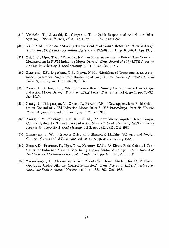
[349]

[350]

[351]

[352]

[353]

[354]

[355]

[356]

[357]

[358]

Yoshioka, T., Miyazaki, K., Okuyama, T., “Quick Response of AC Motor Drive

System,” Hitachi Review, vol 31, no 4, pp. 179-184, Aug 1982.

Yu, L.Y.M., “Constant Starting Torque Control of Wound Rotor Induction Motors,”

Trans. on IEEE Power Apparatus System, vol PAS-89, no 4, pp. 646-651, Apr 1970.

Zai, L.C., Lipo, T.A., “Extended Kalman Filter Approach to Rotor Time Constant

Measurement in PWM Induction Motor Drives,” Conf. Record of 1987 IEEE Industry

Applications Society Annual Meeting, pp. 177-183, Oct 1987.

Zanevskii, E.S., Legotkina, T.S., Litsyn, N.M., “Modeling of Transients in an Auto-

mated System for Programmed Hardening of Long Conical Products,” Elektrtekhnika

(USSR), vol 55, no 11, pp. 36-38, 1985.

Zhang, J., Barton, T.H., “Microprocessor-Based Primary Current Control for a Cage

Induction Motor Drive,” Trans. on IFEE Power Electronics, vol 4, no 1, pp. 73-82,

Jan 1989.

Zhang, J., Thiagarajan, V., Grant, T., Barton, T.H., “New approach to Field Orien-

tation Control of a CSI Induction Motor Drive,” [EE Proceedings, Part B: Electric

Power Applications vol 135, no. 1, pp. 1-7, Jan 1988.

Zhong, H.Y., Messinger, H.P., Rashid, M., “A New Microcomputer Based Torque

Control System for Three Phase Induction Motors,” Conf. Record of IEEE-Industry

Applications Society Annual Meeting, vol 2, pp. 2322-2326, Oct 1989.

Zimmermann, W., “Inverter Drive with Sinusoidal Machine Voltages and Vector

Control (German),” ETZ Archiv, vol 10, no 8, pp. 259-266, Aug 1988.

Zinger, D., Profumo, F., Lipo, T.A., Novotny, D.W., “A Direct Field Oriented Con-

troller for Induction Motor Drives Using Tapped Stator Windings,” Conf. Record of

IEEE-Power Electronics Specialists’ Conference, pp. 855-861, Apr 1988.

Zuckerberger, A., Alexandrovitz, A., “Controller Design Method for CSIM Drives

Operating Under Different Control Strategies,” Conf. Record of IEEE-Industry Ap-

plications Society Annual Meeting, vol 1, pp. 352-362, Oct 1988.

193

Appendix A

MOTOR DRIVE SYSTEM PARAMETERS

Stator resistance Rs = 2.167 2

Rotor resistance R, = 1.782

Stator inductance Ls = 0.2397 H

Rotor inductance L, = 0.2541 H

Mutual inductance Lan = 0.2105 H

Coefficient of viscous friction B = 0.00154 Nm/(rad/sec)

Moment of inertia J = 0.00413 Kg. m?

Number of poles P = 2

Rated output power Po = 1HP

Rated speed N, = 3450 RPM

Rated voltage V, = 230 V

Base value of current Ty = 2.647 A

Base value of torque Ty = 2.064 Nm

Base value of voltage Vp = 187.8 V

Maximum current limit Imar =8A

Maximum torque limit Tmar = 2.064 Nm

PWM switching frequency fe = 1kHz

194

Appendix B

VOLTAGE SENSING ALGORITHM

The voltage sensing algorithm proposed in [141] reconstructs the line voltages from

the base drive control signals and the measured stator currents. It is reproduced in this

Appendix.

B.1 Current Segment Identification

The three stator phase currents are divided into 60 degree segments with each interval

distinctly identifying a mode of operation of the inverter bridge. This is accomplished by

generating six functions, A, B, C, D, E, and F as shown in Fig. B.1 for a phase sequence

of abc. BA1, BA3, and BA5 are the positive half cycles of the a, b, and c stator phase

currents. The other relationships are expressed as follows:

—_—_—_—

BA4 = BAI

BA6 = BA3 (B.1)

BA2 = BA5

and,

A = BAI1.BA5

B = BA2.BA6

C = BA3.BAI1

D = BA4.BA2 (B.2)

195

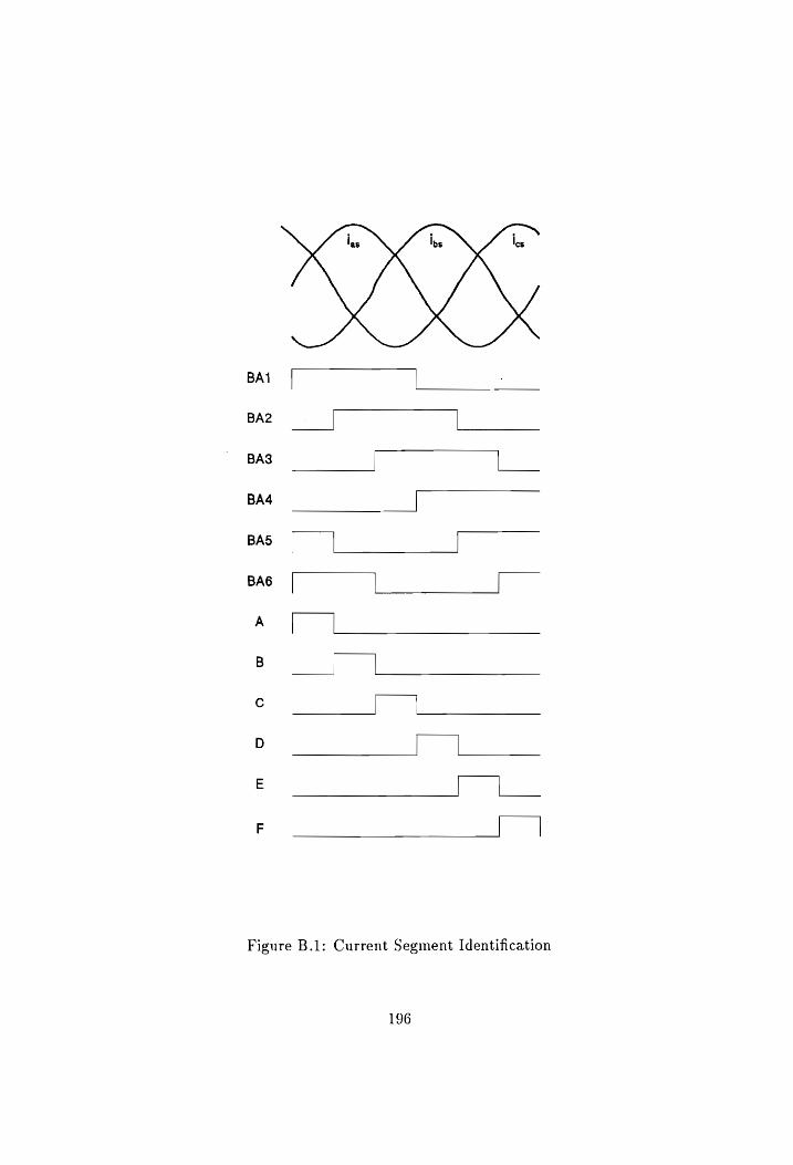
SLWLS BA1

BA2

BA3

BA4

BA5

to LL

to LL

es

|

Bae

[|

| |

LL

LL

PL

J

Figure B.1: Current Segment Identification

196

E = BA5.BA3

F = BA6.BA4

Also, it can be noted from Fig. 5.2 that B1 through B6 are the base drive signals for

the switches T1 through T6.

B.2 Switching Function for Voltage Sensing

For each current segment identified in the previous subsection, the input line voltage is

characterized by a circuit configuration. A step by step derivation of the switching function

for the line voltage V,, with all the different circuit configurations is given in detail in the

following paragraphs. The circuit configurations for the current segments, A through F are

given in Fig. B.2. It can be noted that regardless of the current segment, the line voltage

V.b would be equal to the positive dc bus voltage if the switches T, and Tg are ON. The

switching function for this condition is given as,

(A+ B4+C+D+E+ F).B1.B6 (B.3)

Similarly, Vi, would be equal to the negative dc bus voltage if the switches 73 and 74

are ON. This can be characterized by the following switching function,

(A+B+C+D+E+ F).B3.B4 (B.4)

Fig. B.2(a) corresponds to the circuit configuration for the current segment A. There

are five valid conditions which are given here along with their switching function. If all

the four switches are OFF and the diodes D3 and D4, are freewheeling, V,» is equal to the

negative dc bus voltage. The switching function for this condition is given as,

A.B1.B3.B4.B6 (B.5)

197

+

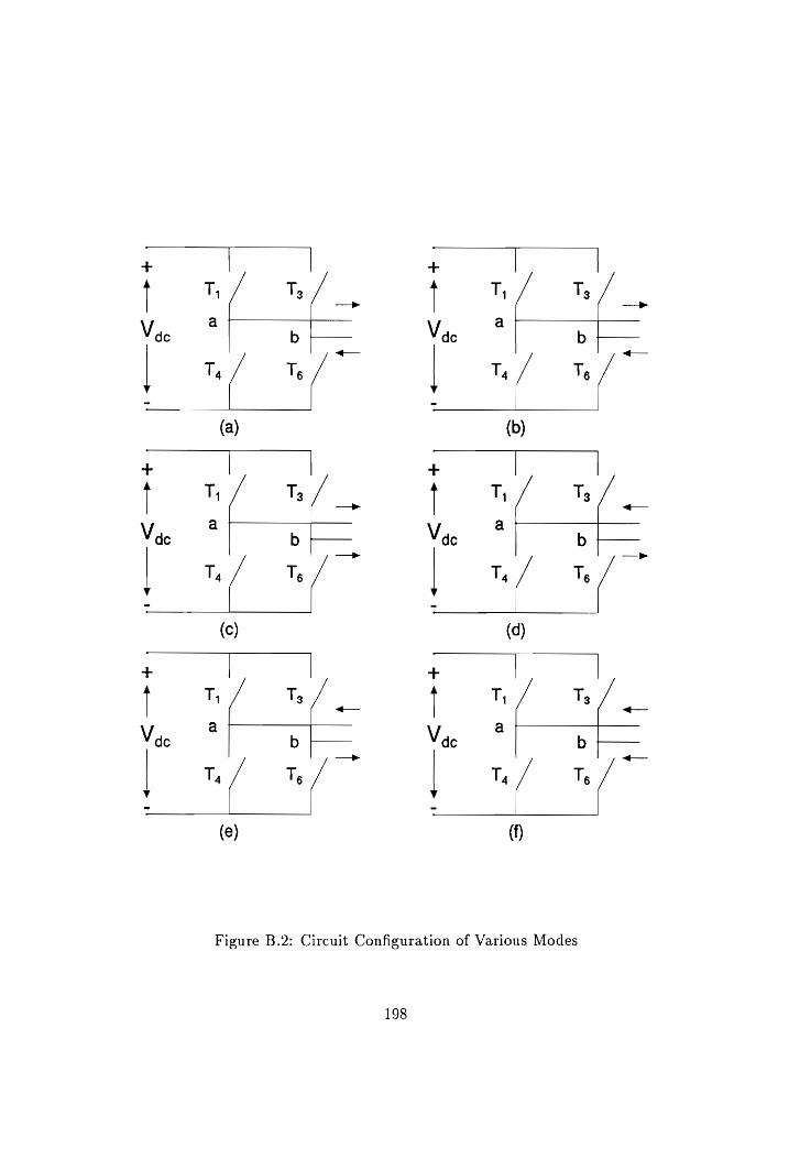
poo ot / Vac 7 b -+——

T, Te

(a)

+ | | | T, Ts _

Ve . b ee

T, ( T,

(c)

+ | | 1 T, Ts _

Vue “ b |__

| T, Ts /

(e)

—

<->

+ Qa

. QO oO

I

a

|

——>

-+

Ve

at

—_ SF

ae —

|

m

— Q

a”

_

iT

de

1<+—— <->

+ _

»

oT]

Gt

+

>» —

D>

ly

—,

=>

wae?

Figure B.2: Circuit Configuration of Various Modes

198

The next valid condition is if T3 is ON and both the diodes D3 and Dy, are freewheeling,

in which case V,, is equal to the negative dc bus voltage. The switching function is given

as,

A.B1.B3.B4.B6 (B.6)

The third condition is if Ty is ON and both the diodes D3 and D4 are freewheeling, and

again V,, is equal to the negative dc bus voltage. The switching function is given as,

A.B1.B3.B4.B6 (B.7)

The fourth condition is if the transistor Tg is ON and the return path is provided through

the freewheeling diode, D4, in which case V,, is equal to zero. The switching function for

this condition is given as,

A.B1.B3.B4.B6 (B.8)

The last is if the transistor JT; is ON and the return path is provided through the

freewheeling diode, D3, in which case V,») is equal to zero. The switching function for this

condition is given as,

A.B1.B3.B4.B6 (B.9)

In a similar fashion, for the current segment B, the valid conditions and the switching

functions are given from Fig. B.2(b) as,

AllOFF: D3,D4 => B.B1.B3.B4.B6 => Vas = —Vac

T3 ON: D3,Dq => B.B1.B3.B4.B6 => Vay = —Vac

T, ON: D3,D, => B.B1.B3.B4.B6 => Voy = —Va- (B.10)

Tg ON: Be,D, => B.B1.B3.B4.B6 >Vy=0

199

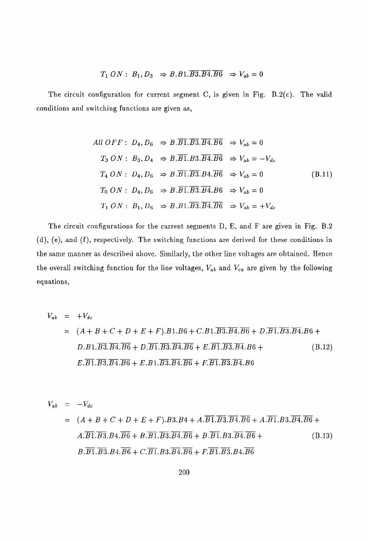
T, ON: B,, D3 => B.B1.B3.B4. 6 => Vap = 0

The circuit configuration for current segment C, is given in Fig. B.2(c).

conditions and switching functions are given as,

AU OFF: D4,Dg => B.BI.B3.B4.B6 => Voy = 0

Tz; ON: B3,Ds => B.B1.B3.B4.B6 => Vy = —Vac

Ty ON: Dg,Dg => B.B1.B3.B4.B6 => Vi» = 0

Ts ON: D4,De => B.B1.B3.B4.B6 => Vay = 0

T,ON: Bi,Dge = B.B1.B3.B4.B6 => Va = +Vac

The valid

(B.11)

The circuit configurations for the current segments D, E, and F are given in Fig. B.2

(d), (e), and (f), respectively. The switching functions are derived for these conditions in

the same manner as described above. Similarly, the other line voltages are obtained. Hence

the overall switching function for the line voltages, V,, and Vea are given by the following

equations,

Vas = +Vac

= (A+ B+C4+D+4+ E+ F).B1.B6 + C.B1.B3.B4.B6 + D.B1.B3.B4.B6 +

D.B1.B3.B4.B6 + D.B1.B3.B4.B6 + E.B1.B3.B4.B6 + (B.12)

E.B1.B3.B4.B6 + E.B1.B3.B4.B6 + F.B1.B3.B4.B6

Vab = —Vae

= (A+B+C4+D+E+4+F).B3.B4 + A.B1.B3.B4.B6 + A.B1.B3.B4.B6 +

A.B1.B3.B4.B6 + B.B1.B3.B4.B6 + B.B1.B3.B4.B6 + (B.13)

B.B1.B3.B4.B6 + C.B1.B3.B4.B6 + F.B1.B3.B4.B6

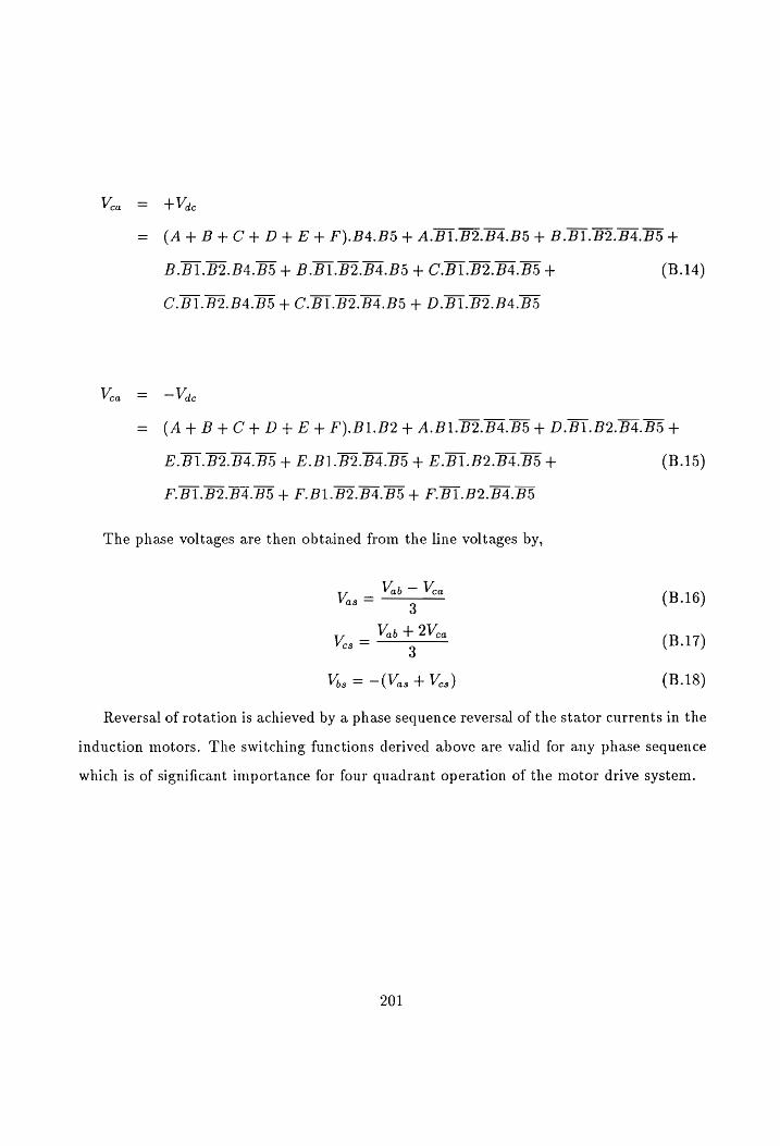
(B.14)

Vea = —Vae

= (A+ B+C+D+E+4+F).B1.B2+ A.B1.B2.B4.B5 + D.B1.B2.B4.B5 +

E.B1.B2.B4.B5 + E.B1.B2.B4.B5 + E.B1.B2.B4.B5 + (B.15)

F.B1.B2.B4.B5 + F.B1.B2.B4.B5 + F.B1.B2.B4.B5

The phase voltages are then obtained from the line voltages by,

Va ~~ Vea Vas = ~ (B.16)

Vao + 2Vea Vig = waht ica (B.17) 3

Vis = —(Vas + Ves) (B.18)

Reversal of rotation is achieved by a phase sequence reversal of the stator currents in the

induction motors. The switching functions derived above are valid for any phase sequence

which is of significant importance for four quadrant operation of the motor drive system.

201

dr

lds

Appendix C

LIST OF SYMBOLS

Gain of the PWM controller

Coefficient of viscous friction

Base frequency

PWM switching frequency

Actual value of A phase current

Commanded value of A phase current

Actual value of B phase current

Commanded value of B phase current

Actual value of C phase current

Commanded value of C phase current

Actual value of field current

Actual value of field current

Actual value of d axis rotor current

Actual value of d axis stator current

Commanded value of d axis stator current

Actual value of g axis rotor current

Actual value of g axis stator current

Commanded value of g axis stator current

Stator phase current

Actual] value of torque current

Actual value of torque current

202

lasn

I,

Imax

bo

NON

ao

7 3

8 nwt

2 3°

Normalized value of A phase stator current

Base value of current

Normalized value of field current

Maximum current limit

Normalized value of torque current

Moment of inertia

Derivative constant

Integral constant

Proportional constant

Torque constant

Equivalent inductance

Mutual inductance

Rotor inductance

Stator inductance

Rated speed

Derivative operator

Number of poles

Airgap power

Rated output power

Normalized value of rotor flux

Rotor resistance

Stator resistance

Base value of torque

Actual value of electromagnetic torque

Commanded value of electromagnetic torque

Normalized value of electromagnetic torque

203

Ves

Vdr

Load torque

Maximum torque limit

Angular value of rotor position

Actual value of A phase voltage

Commanded value of A phase voltage

Actual value of B phase voltage

Commanded value of B phase voltage

Actual value of C phase voltage

Commanded value of C phase voltage

Actual value of d axis rotor voltage

Actual value of d axis stator voltage

Commanded value of d axis stator voltage

Actual value of g axis rotor voltage

Actual value of g axis stator voltage

Commanded value of g axis stator voltage

Normalized value of A phase stator voltage

Base value of voltage

DC link voltage

line to line voltage

Rated voltage

Normalized value of rotor speed

Triggering angle for the rectifier

Current window for hysteresis controller

Field angle

Actual value of angular rotor position

Commanded value of angular rotor position

204

Actual value of slip angle

Commanded value of slip angle

Stator phasor angle with the current vector

Stator phasor angle with the voltage vector

Torque angle with the current vector

Torque angle with the voltage vector

Actual value of d axis rotor flux

Actual value of d axis stator flux

Actual value of g axis rotor flux

Actual value of g axis stator flux

Actual value of rotor flux

Commanded value of rotor flux —,

Base value of speed

Synchronous speed

Actual value of rotor speed

Commanded value of rotor speed

Actual value of rotor speed

Commanded value of rotor speed

205

VITA

Aravind S. Bharadwaj was born in Madras, India on May 21, 1964. He received the

B.E. degree with Honors in Electronics and Communication Engineering from Madurai

Kamaraj University, India in 1985 and the M.S. degree in Electrical Engineering from

Virginia Polytechnic Institute and State University (VPI&SU) in 1987. He joined the Ph.D.

program at VPI&SU in the winter quarter of 1988. His research interests are in the area

of motion control systems and power electronics in which he has published several papers

in international conferences and refereed journals. He is a member of IAS, PES and IES

of IEEE and received the outstanding student member award in 1985. He will be joining

the GM Research Labs soon after graduation to pursue his research in the area of power

electronics. His hobbies include tennis, jogging and travel.

Abruted Ss. Blonaclecy

206