Distributional biases in the analysis of climatechange�

Peter Skotty and Leila Davisz

14th February 2012

Abstract

The economic analysis of global warming is dominated by models basedon optimal growth theory. These representative-agent models have anintrinsic distributional bias in favor of the rich. The bias is compoundedby the use of �revenue-neutrality� in the allocation of emission permits.The result is mitigation recommendations that are biased downwards.

JEL classi�cation: Q13, I3, E1Key words: representative agent, welfare, global warming, inequality.

�An earlier version of this paper was presented at the Analytical Political Economy Work-shop, Queen Mary University of London, May 2011, and at the Adam Smith Seminar, Univer-sity of Hamburg. We thank the participants and Frank Ackerman, Jim Boyce and Liz Stantonfor helpful comments and suggestions. We are grateful also to three anonymous referees. Theirconstructive comments led to signi�cant improvements in this version of the paper.

yDepartment of Economics, University of Massachusetts Amherst; pskott@econs.umass.eduzDepartment of Economics, University of Massachusetts Amherst; leila.davis1@gmail.com

1

1 Introduction

Climate change has strong distributional e¤ects. The expected consequences forpotential crop yields and the likelihood of �ooding or droughts di¤er across re-gions, and the most detrimental e¤ects are expected to occur in poorer regions.Negative health and mortality e¤ects also a¤ect developing countries dispro-portionately. Thus, the Intergovernmental Panel on Climate Change concludes,�The e¤ects of climate change are expected to be greatest in developing coun-tries in terms of loss of life and relative e¤ects on investment and the economy�(IPCC, 2001, p. 8). The severity of these negative e¤ects of climate change inpoor regions is compounded by the fact that �The ability of human systems toadapt to and cope with climate change depends on such factors as wealth, tech-nology, education, information, skills, infrastructure, access to resources, andmanagement capabilities.� Because endowments of these factors are typicallylower in developing countries, poorer regions also �have lesser capacity to adaptand are, therefore, more vulnerable to climate change damages�(p. 8).The uneven distribution of costs and bene�ts is not unique to environmental

change and environmental policy. Policy generally bene�ts some people whileothers are hurt, and Pareto rankings of the outcomes are typically not available.Instead, decisions have to be based on social welfare evaluations that make(implicit or explicit) interpersonal comparisons, weighing up costs and bene�tsso as to arrive at a net result. A standard approach in the economic literatureuses the utility function of a �representative agent�as a social welfare function.In the climate literature, the main debates have centered on the choice of dis-

count rates.1 The Stern Review (Stern 2006) adopted a �prescriptive�approachand argued that on ethical grounds the pure discount rate in the welfare functionshould be close to zero. Nordhaus (2008) and most other studies by contrastuse a �descriptive�approach in which the welfare function of the representativeagent has to be calibrated to �t empirical observations.2 This approach, Nord-haus argues, "does not make a case for the social desirability of the distributionof incomes over space or time under existing conditions". Instead, using thedescriptive approach

The calculations of changes in world welfare arising from e¢ cientclimate-change policies examine potential improvements within thecontext of the existing distribution of income and investments acrossspace and time. (Nordhaus, 2008, p. 174-175)

Assuming that aggregate outcomes can be described consistently by a rep-resentative agent, it may seem reasonable to use this agent�s preferences tomeasure social welfare. This approach has the appearance of neutrality andobjectivity. The analyst does not impose her own preferences but merely takes

1E.g. Chichilnisky (1996), Dasgupta (2011), Davis and Skott (2011), Rezai et al. (2011),Roemer (2011), Stern (2008), Weitzman (2009).

2The �prescriptive�/�descriptive� terminology is used by Arrow at al. (IPCC chapter 4,1996).

1

as given the revealed preferences of the population. Weitzman makes this ar-gument explicitly. Like Nordhaus, he rejects the prescriptive approach of theStern Review, arguing that:

economists understand the di¤erence between their own personalpreferences for apples over oranges and the preferences of others forapples over oranges. Inferring society�s revealed preference ... isnot an easy task in any event ... but at least a good-faith e¤ortat such an inference might have gone some way towards convincingthe public that the economists doing the studies are not drawingconclusions primarily from imposing their own value judgments onthe rest of the world. (Weitzman 2007, p. 712)

According to Weitzman, Nordhaus�s "careful pragmatic modeling throughouthis DICE series of IAMs has long set the standard in this area" (p. 713).3

The use of descriptive representative-agent models is not con�ned to theclimate literature. Models of this kind have been the workhorses of macro-economics since the Lucas revolution of the late 1970s. The explicit welfarecriterion is seen as a strength of the models. Woodford (2003, p. 12; empha-sis added), for instance, suggests that the utility function of the representativeagent "provides a natural objective in terms of which alternative policies shouldbe evaluated", while, according to Blanchard (2008, p. 9, emphasis added),contemporary macro models with formal optimization enable one "to derive op-timal policy based on the correct (within the model) welfare criterion". Mosttellingly, perhaps, the evaluation of outcomes based on the stipulated utilityfunction of the representative agent is usually presented without any argumentor caveat.Although widespread and well-established, there is nothing objective about

this approach to welfare analysis. There is no justi�cation for the implicit claimthat the same function which describes the representative agent can do doubleduty as a measure of social welfare. The representative agent is designed toexplain average behavior and, loosely speaking, this average is determined usingthe economic resources of individual agents as weights. Because a rich agentin�uences aggregate consumption patterns more strongly than a poor agent, thepreferences of the rich agent are given greater weight in the construction of therepresentative agent and hence also in the evaluation of social welfare. In theclimate literature the biases can a¤ect the abatement recommendations fromrepresentative-agent models.At a general level the problems are well known. There is a big literature

on cost-bene�t analysis and the issues are similar.4 Our main contribution inthis paper is to provide simple examples that illustrate the problems and relate

3Despite his endorsement of Nordhaus�s descriptive approach, Weitzman�s conclusions aresimilar to those of Stern: his analysis of risk and the possibility of catastrophic change impliesa low discount rate. In Weitzman�s words, the Stern report may have been "right for thewrong reasons" (2007, p. 724).

4See Ackerman and Heinzerling (2005), Baum (2009), Sen (2000), Stanton (2010) and Stern(2006) for recent discussions with reference to climate change.

2

them to existing IAMs, especially the DICE and RICE models (Nordhaus 2008,Nordhaus and Boyer 2000). We focus on distributional issues that are unrelatedto discounting and other intertemporal questions. Given this purpose, little islost by ignoring the time dimension. Thus, we consider a static setting andassume that all costs and bene�ts occur in the same period.Section 2 examines policy decisions in models with a well-de�ned represen-

tative agent. The models are highly stylized. There are two types of agents andwe assume, in particular, that one good is consumed exclusively by one of thetypes and another good exclusively by the other type. This assumption mayseem restrictive but the goods need not be ordinary goods: they can representthe non-market outcomes in two di¤erent regions. This interpretation and therelevance of the examples is discussed more fully at the end of the section.The examples in Section 2 describe exchange economies without any pro-

duction. Production is introduced in Section 3. The setting is similar to thatof the RICE model. The economy is regionally disaggregated, there is inequal-ity across regions, and the damages from climate change can be calculated indi¤erent ways, with or without some kind of �equity weighting�. However, aunique, optimal level of emissions can be determined independently of distribu-tion if two assumptions are satis�ed: there is a single, homogeneous consumptiongood and this good can be transferred between regions. The crucial role of the�rst assumption (a single �generalized consumption good�) is illustrated by theexamples in Section 2: in these examples the separation between e¢ ciency anddistribution breaks down and policies that maximize a standard measure of realoutput have a strong regressive bias.The transfer assumption is the focus of Section 4 which develops a three good

example. The example builds on Sections 2-3. There is one produced good andtwo non-produced environmental goods. The produced good is tradable andconsumed in all regions; the two environmental goods are non-traded and can-not be transferred. An (extremely restrictive) assumption of perfect substitutionmeans that the �e¢ cient�level of emissions will be uniquely de�ned, despite theexistence of three goods, and the distributional outcome is determined by trans-fers (the allocation of emission permits across regions). The section analyzeshow di¤erent allocation schemes can have adverse distributional consequences:the e¢ cient solution with a reasonable-looking allocation scheme can produce a(utilitarian) welfare loss. Section 5 o¤ers a few concluding remarks.

2 Some simple examples with a well-de�ned rep-resentative agent

Well-behaved preferences at the agent level do not imply that aggregate out-comes behave as if they were generated by an optimizing representative agent.5

5This result, which has been well-known since the work of Debreu (1974), Mantel (1976) andSonnenschein (1972), undermines the claims of modern macro to be built on microeconomicfoundations (Kirman 1992).

3

In some cases, however, a well-de�ned representative agent does exist, and theseare clearly the cases that are most favorable to the representative-agent ap-proach. Our examples focus on cases of this kind. The examples show that,even in these cases, the use of the representative agent for welfare analysis ishighly questionable.6

2.1 A two-good example

Consider an economy with two types of agents, A�types who consume onlygood 1 and B-types who consume only good 2. The total endowment of the twogoods is �q1 and �q2; and all agents have endowment compositions that mirrorthe aggregate composition (changes in relative prices therefore have no distri-butional e¤ects). These assumptions imply that the share of good 1 in totalexpenditure is equal to the share of A-agents in total income (= their share inendowments). If � is the income share of A-agents, aggregate excess demands inthis economy can be derived from the maximization of a Cobb-Douglas utilityfunction,

U = q�1 q1��2 (1)

subject to the aggregate budget constraint p1q1 + p2q2 = p1�q1 + p2�q2. Thus,equation (1) represents the preferences of a representative agent for this econ-omy.Assume that initially �q1 = �q2 = �q and that an opportunity now arises which

would raise �q1 marginally but reduce �q2 by the same amount. Is social welfareincreased by moving from the endowment bundle (�q; �q) to the new bundle (�q +�; �q��)? Using the utility function (1) as the yardstick, the change in welfareis given by

dU = (�q2�q1)��[�

�q2�q1� (1� �)]� = (2�� 1)� (2)

Hence, the analyst must conclude in favor of the policy if � collectively �A�agents have more than 50 percent of the resources. The conclusion doesnot depend on whether a high � re�ects a large share of A�agents in the pop-ulation (with all agents having the same endowment) or a large endowment foreach A�agent (with the same number of A and B agents). In this sense thewelfare criterion is independent of distribution. In general, however, the policyimplications are highly regressive. Consider two economies: they have the sameproportion of A and B agents, but A agents are richer than B agents in oneeconomy while B agents are richer in the other economy. Representative-agentevaluations will give di¤erent conclusions: the analyst will recommend the pol-icy �which favors A agents �in the economy with rich A agents but reject thepolicy when A agents are poor.This two-good example is one of pure con�ict. A and B agents consume

di¤erent goods. Any change in the overall composition of the goods must6According to Kirman (1992), there are cases in which a policy change raises the utility of

all agents but reduces the utility of the representative agent. His argument for this propositionseems unclear, however, and arguably the case with con�icting interests (which Kirman doesnot discuss) is both more interesting and empirically more relevant.

4

bene�t one type and hurt the other. Compensation is impossible, and thereare no Pareto improving changes in the composition of the endowments. Therepresentative-agent approach glosses over this con�ict. It gives a clear andunambiguous policy recommendation: do what is good for the rich. There is anintrinsic bias in favor of the rich.

2.2 A three-good example

Empirically, the consumption sets of the rich and the poor are not completelydisjoint. Some goods are valued by all agents and this opens up the possibilityof compensation and Pareto improving changes. We examine this case using anextended model with three goods.As in the two-good example, there are two types of agent, A and B, and

all agents have the same endowment composition. The new element is theintroduction of a good that is valued and consumed by both types of agent.The preferences of the agents are given by Cobb-Douglas utility functions

UA = q�1Aq1��3A (3)

UB = q�2Bq1��3B (4)

where qij is the consumption of good i by agent j: As in Section 2.1, we let �denote the share of A-agents in total income (YA = �Y; YB = (1� �)Y ).With this combination of preferences and endowments, the consumption

patterns of the two agents satisfy

p1q1A = �YA; p2q2A = 0; p3q3A = (1� �)YA (5)

p1q1B = 0; p2q2B = �YB ; p3q3B = (1� �)YB (6)

Thus, the aggregate demands (q1 = q1A + q1B ; q2 = q2A + q2B ; q3 = q3A + q3B)for the three goods are given by the following equations:

p1q1 = ��Y (7)

p2q2 = (1� �)�Y (8)

p3q3 = (1� �)Y (9)

The demand structure in equations (7)-(9) can be derived from the optimiz-ing behavior of a single representative agent with utility function

U = q��1 q(1��)�2 q1��3 (10)

and budget constraint p1q1 + p2q2 + p3q3 = p1�q1 + p2�q2 + p3�q3 = Y:

2.2.1 Marginal changes

Consider the same policy question as in Section 2.1. Should we increase thesupply of good 1 at the expense of a reduction in the supply of good 2? With

5

a one-for-one tradeo¤ and supplies of the two goods that are equal initially, amarginal change of this kind would have a welfare e¤ect given by

dU = �(�q3�q)1�� [2�� 1] (11)

where �q = �q1 = �q2 is the initial supply of the goods 1 and 2. The conclusion issimilar to the earlier example: implement the policy if � > 0:5:Unlike in the two-good example, the policy decision does not directly prej-

udice the distributional outcome. A�agents are the direct bene�ciaries of thepolicy but the B-agents could be compensated by raising their share of the con-sumption of good 3. Having the third good means that Pareto improvementsbecome possible.There are two extreme cases of Pareto improvements: one in which all the

improvements go to A�agents and one in which only B�agents bene�t. Keep-ing UB unchanged following a marginal increase in q1 (and an equal marginaldecrease in q2) requires

0 = dUB = �UB

q2Bdq2B + (1� �)

UB

q3Bdq3B (12)

ordq3Bd�q1

=�

1� �q3Bq2B

=�

1� �(1� �)�q3

�q1(13)

where we have used d�q2 = �d�q1 (by assumption this is the tradeo¤) and q3B =(1 � �)�q3, q2B = �q2 = �q1 at the initial position (these equilibrium conditionsfollow from (5)-(6)). Since dq3B = �dq3A, we can now derive the gain to theA-agents in the case where dUB = 0 :

dUA = ����(�q3�q1)1�� [2�� 1]d�q1 (14)

Analogously, setting dUA = 0, the increase in q3B and the marginal increasein the utility of B�agents can be found:

dq3Bd�q1

=�

1� �q3Aq1A

=�

1� ���q3�q1

(15)

dUB = (1� �)���( �q3�q1)1�� [2�� 1]d�q1 (16)

The largest improvement in aggregate utility, UA + UB ; comes when allthe net gains are given to the poor B�agents: the symmetric speci�cations ofthe utility functions in equations (3)-(4) imply that poor agents have a highermarginal utility. If one rejects cardinality of the utility function, however, nosigni�cance attaches to the magnitudes of the expressions in equations (14) and(16), and interpersonal comparisons of utility gains become meaningless. Butthe expressions in (13) and (15) still hold without cardinality, and the policygenerates a Pareto improvement if the compensating change dq3B=d�q1 falls inthe interval between the expressions on the right-hand-sides of (13) and (15).

6

2.2.2 Non-marginal change

The analysis in Section 2.2.1 analyzed marginal changes. One can also look forthe optimal amount of good 2 to convert (one-for-one) into good 1. We considerfour di¤erent approaches to this question.

Case I: A �generalized consumption good� The initial equilibrium canbe used to de�ne a generalized consumption good. Using p3 as the numeraire,the demand equations (7)-(9) can be combined with the initial supplies (�q1 =�q2 = �q; �q3) to give the pre-policy equilibrium prices

�p1 =��

1� ��q3�q

(17)

�p2 =(1� �)�1� �

�q3�q

(18)

�p3 = 1 (19)

A generalized good can be de�ned using these weights,

c = �p1q1 + �p2q2 + q3 (20)

If the utility of the representative agent is taken to be an increasing functionof the consumption of this generalized good, policy should aim to maximize�c = �p1�q1 + �p2�q2 + �q3: By assumption, there is a one�for-one transformationbetween goods 1 and 2. The prices of the two goods are di¤erent, however, andusing this criterion the policy-maker should convert all existing supplies of good2 into good 1 if � > 0:5.

Case II: Using the utility function of the representative agent Theanswer in this case is found by maximizing (10) subject to the conditions

q1 + q2 = �q1 + �q2 (21)

q3 = �q3 (22)

The result is(q2q1)�;rep =

1� ��

(23)

Case III: Maximizing UA subject to dUB = 0 Straightforward calcula-tions yield (see the appendix)

(q2q1)�;maxA =

[2(1� �)]1��2� [2(1� �)]1�� =

(1� �)[2(1� �)]� � 1 + � (24)

7

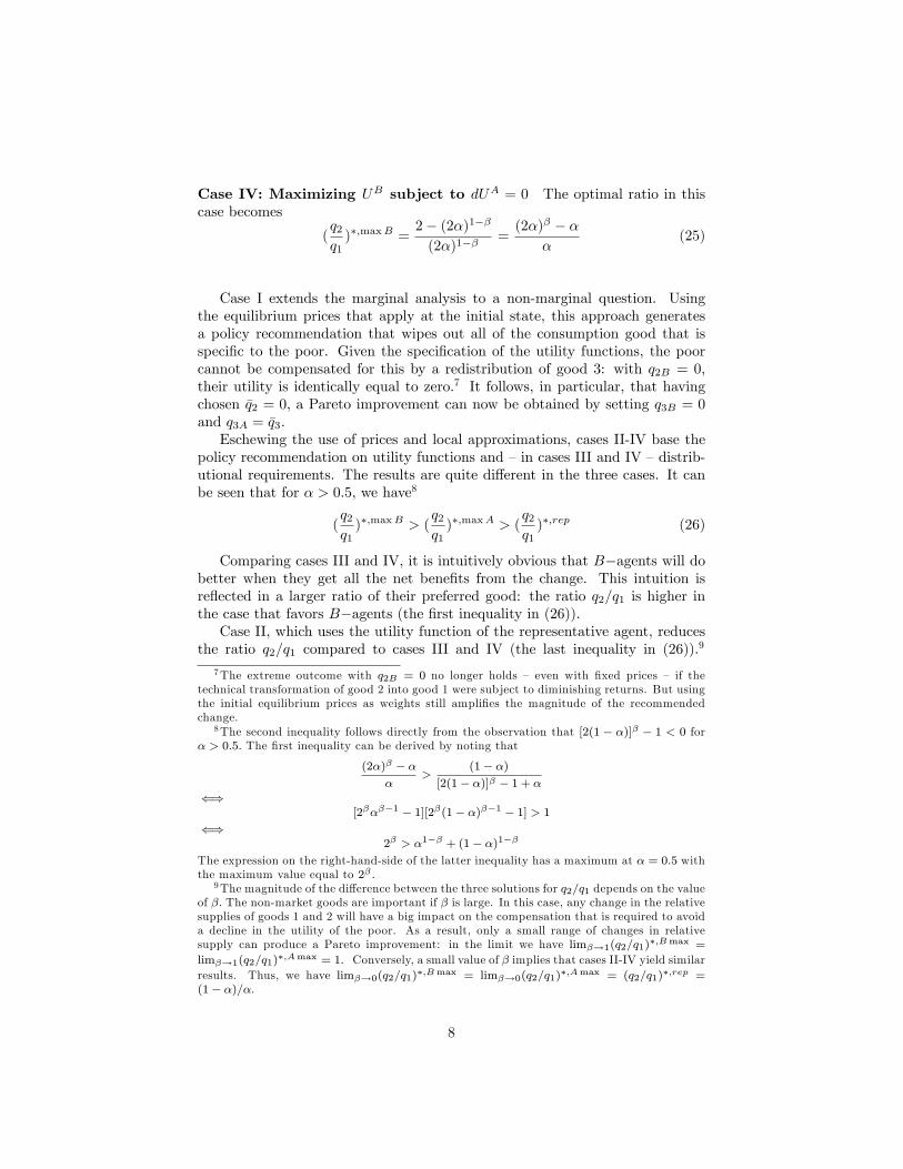
Case IV: Maximizing UB subject to dUA = 0 The optimal ratio in thiscase becomes

(q2q1)�;maxB =

2� (2�)1��(2�)1��

=(2�)� � �

�(25)

Case I extends the marginal analysis to a non-marginal question. Usingthe equilibrium prices that apply at the initial state, this approach generatesa policy recommendation that wipes out all of the consumption good that isspeci�c to the poor. Given the speci�cation of the utility functions, the poorcannot be compensated for this by a redistribution of good 3: with q2B = 0;their utility is identically equal to zero.7 It follows, in particular, that havingchosen �q2 = 0; a Pareto improvement can now be obtained by setting q3B = 0and q3A = �q3:Eschewing the use of prices and local approximations, cases II-IV base the

policy recommendation on utility functions and �in cases III and IV �distrib-utional requirements. The results are quite di¤erent in the three cases. It canbe seen that for � > 0:5, we have8

(q2q1)�;maxB > (

q2q1)�;maxA > (

q2q1)�;rep (26)

Comparing cases III and IV, it is intuitively obvious that B�agents will dobetter when they get all the net bene�ts from the change. This intuition isre�ected in a larger ratio of their preferred good: the ratio q2=q1 is higher inthe case that favors B�agents (the �rst inequality in (26)).Case II, which uses the utility function of the representative agent, reduces

the ratio q2=q1 compared to cases III and IV (the last inequality in (26)):9

7The extreme outcome with q2B = 0 no longer holds � even with �xed prices � if thetechnical transformation of good 2 into good 1 were subject to diminishing returns. But usingthe initial equilibrium prices as weights still ampli�es the magnitude of the recommendedchange.

8The second inequality follows directly from the observation that [2(1 � �)]� � 1 < 0 for� > 0:5: The �rst inequality can be derived by noting that

(2�)� � ��

>(1� �)

[2(1� �)]� � 1 + �()

[2����1 � 1][2�(1� �)��1 � 1] > 1()

2� > �1�� + (1� �)1��

The expression on the right-hand-side of the latter inequality has a maximum at � = 0:5 withthe maximum value equal to 2� :

9The magnitude of the di¤erence between the three solutions for q2=q1 depends on the valueof �: The non-market goods are important if � is large. In this case, any change in the relativesupplies of goods 1 and 2 will have a big impact on the compensation that is required to avoida decline in the utility of the poor. As a result, only a small range of changes in relativesupply can produce a Pareto improvement: in the limit we have lim�!1(q2=q1)

�;Bmax =

lim�!1(q2=q1)�;Amax = 1: Conversely, a small value of � implies that cases II-IV yield similar

results. Thus, we have lim�!0(q2=q1)�;Bmax = lim�!0(q2=q1)

�;Amax = (q2=q1)�;rep =(1� �)=�.

8

The poor B�agents are hurt by this reduction. In principle, they could becompensated by an increase in their share of good 3. If the post-policy outcomeis to be Pareto e¢ cient, however, there can be no such compensating increase.To see this, note that the composition of goods 1 and 2 is chosen so as to matchthe initial equilibrium outcome for q3B=q3A:10 Pareto e¢ ciency requires thatq2=q1 = q3B=q3A; and it follows that �having set the supply ratio �q2=�q1 equalto the initial consumption ratio for good 3 �this initial equilibrium compositionof good-3 consumption must be maintained if the new allocation is to be e¢ cient.Policies that combine the case-II value of q2=q1 with redistribution of good 3may achieve a Pareto improvement, but they will not be Pareto e¢ cient.In short, in this example the representative-agent analysis leads to an out-

come that is either ine¢ cient or distributionally regressive. This conclusion isrelated to the dependence of the descriptive representative agent on the distrib-ution of income. If we change the distribution of income in order to compensatethe poor in region B for a decline in their consumption of the non-market goodthen the appropriate de�nition of the representative agent is a¤ected: the shareof A-agents (�) is a parameter in the representative agent�s utility function,equation (10). This result illustrates one of the problems with the Lucas-inspiredprogram of �micro-founded�macroeconomics. The microeconomic foundationsfor macroeconomics were needed, Lucas argued, because the preferences of indi-vidual agents could be taken as invariant to changes in economic policy. But asshown by the example, distributional changes (a change in the share of the A-agents) imply that the representative agent has to be re-de�ned. Real-world pol-icy changes invariably have distributional consequences. Hence, contemporarymacro is itself subject to a �Lucas critique�: the preferences of the representativeagent are not structurally invariant.

2.3 Discussion

The two- and three-good examples in Sections 2.1-2.2 have well-de�ned repre-sentative agents. Changes in relative prices have no distributional e¤ects, butthis does not eliminate distributional con�icts. The preferences and the compo-sition of the consumption bundles di¤er across agents, and there are potentialcon�icts over both the distribution and composition of the endowment bundles.The examples are simple and abstract, and they may seem far removed

from the climate debate. The assumption that good 1 is consumed only byA-types and good 2 only by B-types may appear particularly restrictive. Thisconcern would be reasonable if the goods were thought of as ordinary, tradedgoods. But another interpretation is possible. Many of the important e¤ects ofclimate change are outside the market sphere. Health and mortality e¤ects areobvious examples, but broader social implications (including migration and thepossibility of wars and other upheavals in the wake of strong regional e¤ects)fall in this category too. The non-market e¤ects of climate change are unevenly

10This happens because both the parameters of the representative agent�s utility functionand the consumption ratio q3B=q3A are determined by the distribution of income.

9

distributed, and goods 1 and 2 can be interpreted as the non-market outcomesin two di¤erent regions, a rich A region and a poor B region.An interpretation which has good 1 representing the health of people in

region A and good 2 the health of people in region B may seem inconsistentwith the assumption that all agents receive endowment bundles with the samecomposition. The utility functions, however, mean that A-agents get no utilityfrom the consumption of good 2 and B-agents no utility from good 1. With thisspeci�cation of preferences, the outcome of an economy in which all three goodsare traded and the initial compositions are the same across agents is isomorphicto the outcome in an economy in which all good-1 endowments are given to Aagents, all good-2 endowments are given to the B-agents, and only good 3 istradable. Neither economy will see any trade in good 3, and both economieswill have A-agents consume the total supply of good 1 and B-agents the totalsupply of good 2.The damages of climate change fall disproportionately on poor regions while

the bene�ts from continued greenhouse gas emissions accrue more strongly toricher regions. A stylized version of this distributional pattern can be capturedin the 3-good example by associating an increase in emissions with an increasein the supply of good 1 at the expense of good 2.

3 Integrated assessment models

3.1 The setting

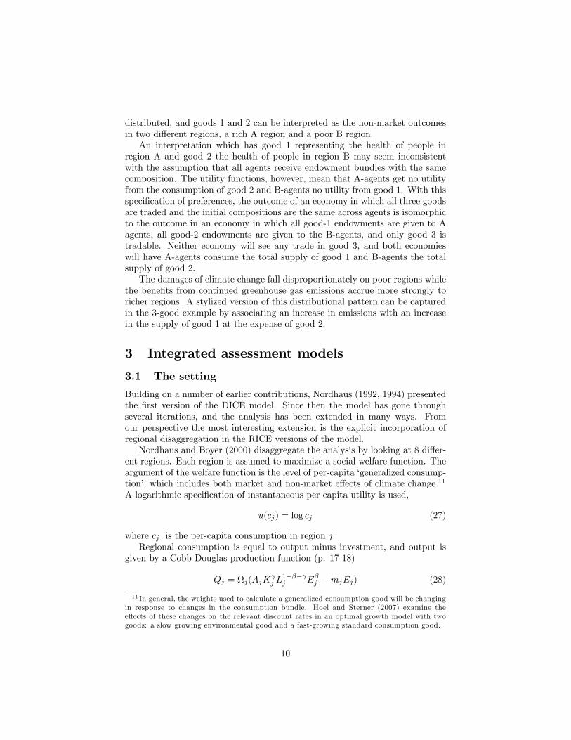
Building on a number of earlier contributions, Nordhaus (1992, 1994) presentedthe �rst version of the DICE model. Since then the model has gone throughseveral iterations, and the analysis has been extended in many ways. Fromour perspective the most interesting extension is the explicit incorporation ofregional disaggregation in the RICE versions of the model.Nordhaus and Boyer (2000) disaggregate the analysis by looking at 8 di¤er-

ent regions. Each region is assumed to maximize a social welfare function. Theargument of the welfare function is the level of per-capita �generalized consump-tion�, which includes both market and non-market e¤ects of climate change.11

A logarithmic speci�cation of instantaneous per capita utility is used,

u(cj) = log cj (27)

where cj is the per-capita consumption in region j:Regional consumption is equal to output minus investment, and output is

given by a Cobb-Douglas production function (p. 17-18)

Qj = j(AjK j L

1��� j E�j �mjEj) (28)

11 In general, the weights used to calculate a generalized consumption good will be changingin response to changes in the consumption bundle. Hoel and Sterner (2007) examine thee¤ects of these changes on the relevant discount rates in an optimal growth model with twogoods: a slow growing environmental good and a fast-growing standard consumption good.

10

where E is carbon-energy and m is the cost of this intermediate input; Q isoutput, K and L are capital and labor, and A represents the level of technol-ogy. The regional estimate of represents the proportional loss of regionaloutput from climate change. This loss depends on the average temperature,and temperatures in turn are related to emissions.The regional loss varies signi�cantly across regions. A rise of 2.5 degree

Celsius in average temperatures produces an estimated output loss of 0.45 per-cent in the US, while the estimated loss of output in the group of low-incomecountries amounts to 2.64 percent.The global loss can be found as a weighted average of the regional losses, and

two distinct measures are presented: one using output weights and one usingpopulation weights.

Output loss Output is treated as homogeneous in the model. Generalizedoutput (and consumption) in region i can be transformed one-for-one into gen-eralized output in region j. Thus, aggregate output is given by

Q =X

Qj (29)

and the �rst measure of global damages is a standard expression for the pro-portional output loss:

dQ

Q=X dQj

Q=X Qj

Q

dQjQj

=X Qj

Q

djj

(30)

Welfare loss An indicator of output loss does not give an accurate picture ofthe welfare implications. Equation (27) implies that marginal utility is decliningin consumption, and an additional unit of consumption does not provide thesame utility gain to a rich person as to a poor person. Population weights canbe seen as a way of adjusting for this.Nordhaus and Boyer do not discuss the population weights in any detail,

but the population-weighted output loss approximates the welfare implicationsof the damages when the utility function is logarithmic. A utilitarian approachde�nes total welfare as the population weighted average of regional welfare,

W =X Nj

Nu(cj) (31)

where Nj and N denote regional and global population. With a logarithmicutility function it follows that the change in welfare can be written

dW =X Nj

Nu0(cj)dcj =

X NjN

dcjcj

=X Nj

N

djj

(32)

where the last equality follows from an assumption of proportionality betweenoutput and consumption (and from the calculation of the loss for given valuesof A;K;L;E).

11

Because damages are higher and consumption is lower in poor regions, popu-lation weighted measures produce higher estimates of aggregate damages. Thus,in Nordhaus and Boyer�s model, the use of population weights increases esti-mates of the damages resulting from a �ve degree Celsius increase in globalmean temperature from six percent to eight percent of GDP. Similarly, Tol(2002) �nds that �equity-weighted� estimates lead to a doubling of projecteddamages associated with a 5 degree increase in temperatures. In general, thereis widespread agreement among economists that some kind of weighting canbe used to capture the welfare e¤ects of an uneven distribution of damages; asan example, the Stern review seems to endorse this approach (Stern, 2006, pp.148-149).

Discussion The utilitarian approach to welfare is controversial and raises is-sues that are beyond the scope of this paper. Staying within the standardoptimal-growth framework, there is no consensus on the de�nition of �equity�.The Nordhaus and Boyer adjustment invites two obvious (and well-known)points. The disaggregation, �rst, is not taken very far. Increasing the num-ber of regions will almost certainly raise the population weighted estimate ofdamages. Moreover, within each region the damages are likely to a¤ect thepoor more strongly than the rich which � if taken into account �would raisethe estimates even further.12

The second problem is more technical. The population weighting providesa good (local) approximation of welfare changes if the utility function u(cj)is logarithmic. The logarithmic speci�cation is the limiting case of a generalCRRA utility function, u(cj) = (c1��j � 1)=(1 � �), with � ! 1. It is widelysuggested, however, that a speci�cation with � > 1 gives a better �t for thepreferences of the representative agent, and a higher value of � implies thatmarginal utility falls o¤ more rapidly as consumption increases.13 As a result,the outcomes for the poor need to be given even greater weight in order to getan estimate of the total welfare loss. Formally, if u(cj) = (c

1��j � 1)=(1� �),

dW =X Nj

Nu0(cj)dcj =

X NjNc��j dcj =

X NjNc��+1j

dcjcj

=X Nj

Nc��+1j

djj(33)

As an example, consider a three-region case: a rich region with income at 2 anddamages at 1 percent, a middle income region with income at 1 and damages at2 percent, and a poor region with income at 0.5 and damages at 3 percent, andassume that population is evenly divided across the three regions. The incomeweighted output loss is 1.57 percent (equation (30)); the welfare loss, however,is 2 percent if the utility function is logarithmic (in which case the welfare lossequals the population weighted output loss, equation (32)) and 2.83 percent if� = 2 (equation (33)):14

12See Antho¤ et al. (2010) for a recent discussion.13Nordhaus (2008) assumes � = 2:14One may note also that if � > 1; the welfare loss will depend on the degree of inequality,

12

Azar and Sterner (1996) discuss the e¤ects of disaggregation on the welfareloss; see also Antho¤ et al. (2009). Nordhaus and Boyer, however, do notpursue these issues, and there is no need for them to do this. Their approachimplies that equity weighting becomes largely irrelevant for the calculation ofthe e¢ cient level of mitigation.

3.2 The �optimal solution�

Consider a true one-good world in which the utility of individuals depends ex-clusively on their consumption of this good. In this world e¢ ciency requiresthat the amount of the good be made as large as possible; in general this con-dition also determines where the production (and emissions) should take place.Once total consumption has been maximized, the outcome will be Pareto ef-�cient no matter how the good is distributed among regions and individuals.Thus, the optimal amount of mitigation can be found without any reference todistribution. This independence of e¢ ciency from distribution does not implythat distribution is unimportant from a welfare perspective. But in a one-goodworld, equity concerns are separate from e¢ ciency. Equity-weighted damagescan be calculated to illustrate the di¤erential impact of global warming, butthey play no role in the derivation of the optimal level of emissions.15

The Nordhaus-Boyer model reduces all outcomes to a single good, �general-ized consumption�. But their model does not describe a true one-good world.The generalized consumption good is constructed using relative prices associ-ated with an initial equilibrium. In this respect the Nordhaus-Boyer argument�ts case I in Section 2.2.As shown in Section 2.2, the maximization of the total supply of generalized

consumption shifts the policy recommendations further in the interest of therich regions than would be justi�ed by a representative-agent analysis whichitself is biased in favor of the rich. Moreover, e¢ ciency cannot be separatedfrom distribution if the one-good assumption is abandoned. The examples insection 2.2 illustrate this general point: the representative-agent analysis in caseII led to a recommendation that was only e¢ cient for a particular distributionof income.

even if all regions su¤er the same proportional damage. Thus, if dj=j = d=

dW =X Nj

Nc��+1j

dj

j=d

X Nj

Nc��+1j � d

c��+1

with equality i¤ cj = c for all j:15Assuming that the consumption good can be transferred. See Chichilnisky and Heal

(1993) for an analysis of cases where no such transfer is possible.

13

4 The case of perfect substitution

4.1 Compensation

The Nordhaus-Boyer approach is theoretically valid in the special case of perfectsubstitution between goods 1 and 3 for A-agents and between goods 2 and 3for B-agents (this special case e¤ectively means that we have a true one-goodworld). The assumption of perfect substitution is extremely restrictive and hasno empirical support, but let us accept it for the sake of the argument.Having found the optimal level of emissions, the distribution of the avail-

able amount of generalized consumption across regions has to be determined. Aradical utilitarian approach would maximize the sum of utility. Using the same(cardinal) utility functions for rich and poor agents, the distributional conse-quences would be immense. If global mitigation e¤orts are linked strongly withdramatic redistribution, however, it may be di¢ cult to get the rich countries toparticipate. Recognizing this, Ackerman et al. (2010) �who adopt a utilitarianapproach �temper their recommendations by including several constraints, oneof them that consumption in the rich countries must not decline in absoluteterms.A focus on Pareto improvements would seem to be in line with Nordhaus�s

stated objective to "examine potential improvements within the existing distri-bution of income" (cf. above p. 1). In terms of our examples in Section 2, therelevant outcomes then fall in the range between those of cases III and IV, withequity concerns presumably tilting the choice towards case IV which favors thepoor.16

Nordhaus and Boyer do not discuss the compensation issue in any detail.Implicitly, however, their position on distribution is re�ected in the allocationof emission permits. Emissions can be controlled through tradable permits, andthe total number of permits is determined by the e¢ ciency requirement. Butthe initial allocation of these permits has distributional e¤ects.17 The issues canbe illustrated using an extended version of the models in Section 2.

4.2 3-good example with production

Building on the 3-good example in Section 2, we de�ne the regional welfare asa function of the consumption of goods 1 and 3 in region A and goods 2 and3 in region B. Unlike in Section 2, however, it is assumed that there is perfectsubstitution. A-agents are willing to substitute one-for-one between goods 1 and3 and their utility is determined by the sum of their consumption of goods 1 and3; B-agents�utility, analogously, is determined by the sum of their consumption

16 IPCC (1996, chapter 3) surveys the literature on equity in the distribution of emissionsand abatement costs.17Note that these distributional e¤ects occur both within and across countries; see, for

example, Brenner et al 2007 for a discussion of distributional e¤ects within China.

14

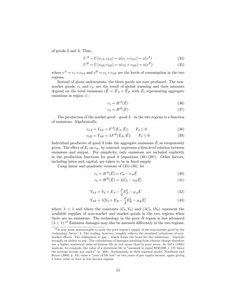
of goods 2 and 3. Thus,

UA = U(c1A; c3A) = u(c1 + c3A) = u(cA) (34)

UB = U(c2B ; c3B) = u(c2 + c3B) = u(cB) (35)

where cA = c1+ c3A and cB = c2+ c3B are the levels of consumption in the tworegions.Instead of given endowments, the three goods are now produced. The non-

market goods, c1 and c2, are the result of global warming and their amountsdepend on the total emissions ( �E = �EA + �EB with �Ei representing aggregateemissions in region i) :

c1 = HA( �E) (36)

c2 = HB( �E) (37)

The production of the market good �good 3 �in the two regions is a functionof emissions. Algebraically,

c3A = Y3A = FA(EA; �E); F2 � 0 (38)

c3B = Y3B = �FB(EB ; �E); F2 � 0 (39)

Individual producers of good 3 take the aggregate emissions �E as exogenouslygiven. The e¤ect of Ei on c3i, by contrast, expresses a �rm-level relation betweenemissions and output. For simplicity, only emissions are included explicitlyin the production functions for good 3 (equations (38)-(39)). Other factors,including labor and capital, are taken to be in �xed supply.Using linear and quadratic versions of (35)-(39), let

c1 = HA( �E) = C0 � �A �E (40)

c2 = HB( �E) = �[C0 � �B �E] (41)

Y3A = Y0 + EA ��

2E2A � �A �E (42)

Y3B = �[Y0 + EB ��

2E2B � �B �E] (43)

where � < 1 and where the constants (C0; Y0) and (�C0; �Y0) represent theavailable supplies of non-market and market goods in the two regions whenthere are no emissions. The technology in the poor B region is less advanced(� < 1):18 Emission damages may also be assessed di¤erently in the two regions,

18 It may seem unreasonable to scale the poor region�s supply of the non-market good by the�technology factor��: The scaling, however, roughly re�ects the standard valuations of non-market e¤ects. The willingness to pay �which forms the basis for the valuations � dependsstrongly on ability to pay. The calculations of damages resulting from climate change thereforeuse a higher statistical value of human life in rich areas than in poor areas. In Tol�s (1995)analysis, for example, the value of a statistical life is "assumed to equal $250,000 + 175 timesthe average income per capita�(p. 369). Analogously, in their regional model, Nordhaus andBoyer (2000, p. 82) value a "year of life lost" at two years of per capita income, again givinga lower value to lives in low income regions.

15

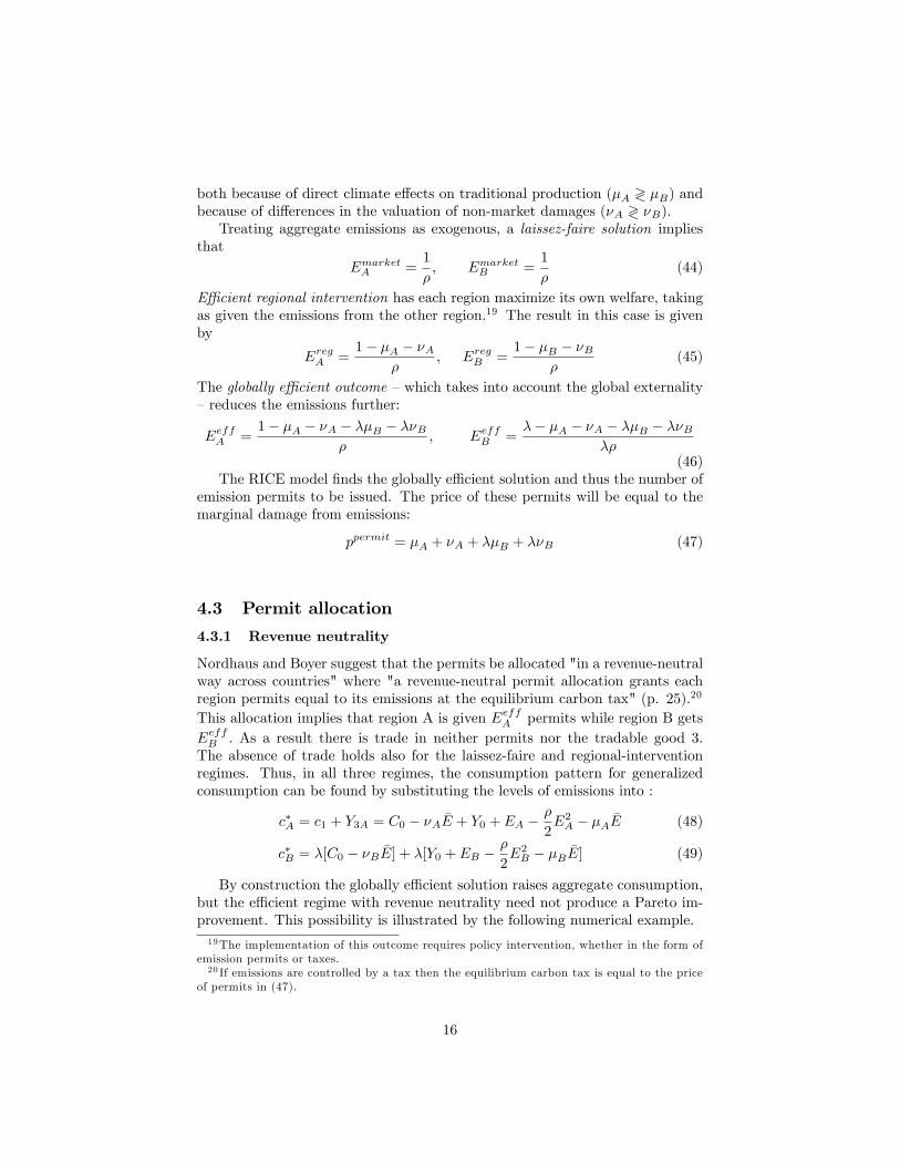
both because of direct climate e¤ects on traditional production (�A ? �B) andbecause of di¤erences in the valuation of non-market damages (�A ? �B).Treating aggregate emissions as exogenous, a laissez-faire solution implies

thatEmarketA =

1

�; EmarketB =

1

�(44)

E¢ cient regional intervention has each region maximize its own welfare, takingas given the emissions from the other region.19 The result in this case is givenby

EregA =1� �A � �A

�; EregB =

1� �B � �B�

(45)

The globally e¢ cient outcome �which takes into account the global externality�reduces the emissions further:

EeffA =1� �A � �A � ��B � ��B

�; EeffB =

�� �A � �A � ��B � ��B��

(46)The RICE model �nds the globally e¢ cient solution and thus the number of

emission permits to be issued. The price of these permits will be equal to themarginal damage from emissions:

ppermit = �A + �A + ��B + ��B (47)

4.3 Permit allocation

4.3.1 Revenue neutrality

Nordhaus and Boyer suggest that the permits be allocated "in a revenue-neutralway across countries" where "a revenue-neutral permit allocation grants eachregion permits equal to its emissions at the equilibrium carbon tax" (p. 25).20

This allocation implies that region A is given EeffA permits while region B getsEeffB : As a result there is trade in neither permits nor the tradable good 3.The absence of trade holds also for the laissez-faire and regional-interventionregimes. Thus, in all three regimes, the consumption pattern for generalizedconsumption can be found by substituting the levels of emissions into :

c�A = c1 + Y3A = C0 � �A �E + Y0 + EA ��

2E2A � �A �E (48)

c�B = �[C0 � �B �E] + �[Y0 + EB ��

2E2B � �B �E] (49)

By construction the globally e¢ cient solution raises aggregate consumption,but the e¢ cient regime with revenue neutrality need not produce a Pareto im-provement. This possibility is illustrated by the following numerical example.19The implementation of this outcome requires policy intervention, whether in the form of

emission permits or taxes.20 If emissions are controlled by a tax then the equilibrium carbon tax is equal to the price

of permits in (47).

16

Example 1 � = 1=3; � = 0:1; �A = �B = �A = �B = 0:05With these parameter values the income of the poor region declines in the

e¢ cient solution compared to both laissez-faire and regional intervention (seeTable 1). A revenue neutral allocation of permits means that no compensationwill take place, and if the utility functions are su¢ ciently concave the overalle¤ect on social welfare will be negative (assuming a utilitarian measure of socialwelfare). The increase in e¢ ciency has produced greater inequality and a declinein aggregate welfare.

The intuition behind the outcome in example 1 is straightforward. Therich countries may have large emissions, but they are also likely to be e¢ cientproducers (they have gained this energy e¢ ciency partly through past learning-by-doing which itself involved emissions). Hence, it becomes e¢ cient to locateproduction in the rich countries, and revenue neutrality means that there is nocompensation to the rest of the world, as long as the rich-country emissions donot exceed the e¢ cient level. In fact, revenue neutrality means that one canhave the paradoxical outcome in which a poor region that has low emissionsand in�icts little damage is required to compensate the rich simply because itmay have failed to reduce its (low) emissions to the e¢ cient level (which is evenlower because the region is poor).Example 1 assumes symmetry in damages. The bene�ts to the poor from

reducing emissions increase if the damages fall more heavily on the poor. Thisis illustrated by example 2 which assumes symmetry in productivity (� = 1)

17

but di¤erences in damages (�A < �B ; �A < �B). The example is calibrated togive the same relative consumption as example 1 in the laissez-faire case.

Example 2 � = 1; � = 0:1; �A = �A = 0:05; �B = �B = 0:1This parameter constellation implies that the income of the poor region

increases in the e¢ cient scenario relative to the scenario with regional e¢ ciencyand a fortiori relative to laissez faire (Table 1). Most of the bene�ts in thisexample accrue to the poor region.

4.3.2 Damage neutrality

Revenue neutrality can produce outcomes that are distinctly non-neutral. Theunderlying principle also seems peculiar: why not give the permits to the regionsthat su¤er the damage rather than to those that in�ict the damage? Followinga rights-based line of reasoning, the net compensation from one region to therest of the world could be calculated as the di¤erence between (i) the estimatedglobal damages from the region�s emissions and (ii) the estimated damage fromglobal emissions on the regions own net output.21

In a damage-neutral scheme the permits are allocated to the regions in pro-portion to the damages that they su¤er. In terms of the two numerical examples,a damage neutral allocation implies the following net transfer from A to B:

� = ppermit[EA ��A + �A

�A + �A + �(�B + �B)(EA + EB)]

= �(�B + �B)EA � (�A + �A)EB (50)

These damage neutral transfers bene�t the poor region when the parametersare as in example 2 (see Table 1). With the parameters from example 1, how-ever, the poor region does worse than under revenue neutrality (Table 1). Thisdeterioration of the outcome for the poor region illustrates an important point:the fairness of a damage neutral allocation depends on the calculation of thedamages. The allocation can be very unfair if market prices and willingness topay are used to estimate damages. Suppose for instance that (i) the only dam-ages are loss of life, (ii) the same number of lives is lost in each of two regions,and (iii) the regions produce roughly the same level of emissions. Under thesecircumstances, the poor region will be required to compensate the rich sincelives are valued more highly in the rich region.

4.3.3 Population neutrality

As a parallel to Nordhaus and Boyer�s use of population weights in the calcu-lation of equity-weighted damages, a population-neutral allocation of permitsdistribute the permits in proportion to population.22 In our simple model, if theA and B regions have the same size population, transfers based on this principle

21Damage-neutrality corresponds to the �compensation�case in Antho¤ and Tol (2010).22For advocacy and discussion of �population neutrality�, see Narain and Riddle (2007).

18

bene�t the poor when the parameters are as in example 1; using example-2 pa-rameters, however, the poor do no better than under revenue neutrality (Table1).

4.4 Discussion

The numerical examples in this section consider three di¤erent permit alloca-tions. All three allocations can be considered �neutral�in some sense.23 Theirimplications, however, are very di¤erent. The examples are stylized but theyserve to illustrate why e¢ cient allocations may fail to produce Pareto improve-ments, even when paired with seemingly reasonable principles of permit alloca-tion.The examples point to a general issue. There is a tension in much of the eco-

nomic literature on climate change between utilitarian notions and an emphasison �e¢ ciency�and Pareto-optimality. E¢ cient policies may produce a welfareloss, from a utilitarian perspective, if they hurt the poor. Conversely, welfaregains can be obtained if �starting from an e¢ cient solution with inequality �the poor regions are allowed to increase their emissions EB with a concomitantreduction in rich-region emissions EA: The reason is obvious: this reallocationof emissions redistributes income towards the poor who have a high marginalutility, and if the initial allocation is e¢ cient, the �rst-order welfare gain domi-nates the second-order e¢ ciency loss. From a welfare perspective, an ine¢ cientoutcome can be better than many e¢ cient solutions.Ine¢ cient reallocations of emissions may not be the best way to implement

a welfare enhancing redistribution of income. A standard economic argumentsuggests that if redistribution is desired, it should be implemented without cre-ating unnecessary distortions. There is something disingenuous, however, aboutan approach that (i) insists on mitigation e¢ ciency, whatever the distributionalconsequences, (ii) argues that compensation must also be done e¢ ciently, but(iii) fails to provide a mechanism to ensure that compensation will in fact bemade and (iv) introduces revenue-neutral allocations which cannot be justi�edon e¢ ciency grounds and which (almost certainly) are distributionally regres-sive.The fact that compensation payments from the rich to the poor could po-

tentially produce a Pareto improvement is largely irrelevant. As argued by Sen(2000),

There is a real motivational tension in the use of the logic ofcompensation for reading social welfare. If compensations are actu-ally paid, then of course we do not need the compensation criterion,since the actual outcome already includes the paid compensationsand can be judged without reference to compensation tests.... On

23Another option, founded in the language of the UN Framework Convention on ClimateChange, is to allocate rights across nations on the basis of the two principles of responsibilityand capacity; see the �greenhouse development rights�proposal by Baer, et al (2008) for anexample translating these two principles into an operational plan.

19

the other hand, if compensations are not paid, it is not at all clearin what sense it can be said that this is a social improvement.... Thecompensation tests are either redundant or unconvincing (p. 947).

5 Conclusion

It is sometimes suggested that the science behind global warming may be weakbut that the economics of the integrated assessment models is well-establishedand sound. We are not in position to evaluate the science but well-establishedas it may be, the economics is questionable.The descriptive representative-agent approach is not value free. It has an

intrinsic regressive bias, and this bias also has implications for the calculations of�optimal emissions�. The damages of climate change are expected to be relativelyconcentrated in poor regions while the bene�ts from continued greenhouse gasemissions accrue more strongly to richer regions. As a result, the maintenanceof standards of living in the rich areas is overemphasized at the expense ofenvironmental degradation. The policy that is best for the representative agentwill impose relatively lower utility costs on rich regions of world than would bejusti�ed by evaluations that are sensitive to distributional considerations.There are no objective, value-free answers to normative questions that in-

volve distributional con�icts. Any attempt to derive an �optimal� amount ofemissions is contingent on some underlying �implicit or explicit �value judg-ment. The descriptive representative-agent approach tries to avoid judgmentsof this kind. But not wanting to take sides easily leads to a de facto sidingwith the rich. Regressive biases are introduced into the IAMs through the useof descriptive representative agents, the reduction of consumption bundles to a�generalized consumption good�, and the allocation of emission permits.

Appendix: Derivation of equation (24)

The pre-policy solution has q2B = �q and q3B = (1 � �)�q3: Thus, the policyproblem in this case is to maximize UA = q�1 q

1��3A subject to the constraints

q1 + q2 = 2�q (A.1)

q3A + q3B = �q3 (A.2)

UB = q�2 q1��3B = �q�((1� �)�q3)1�� (A.3)

Substituting (51) and (52) in (53) the problem can be re-written as

max q�1 q1��3A (A.4)

s:t (A.5)

(2�q � q1)�(�q3 � q3A)1�� = �q�((1� �)�q3)1��

20

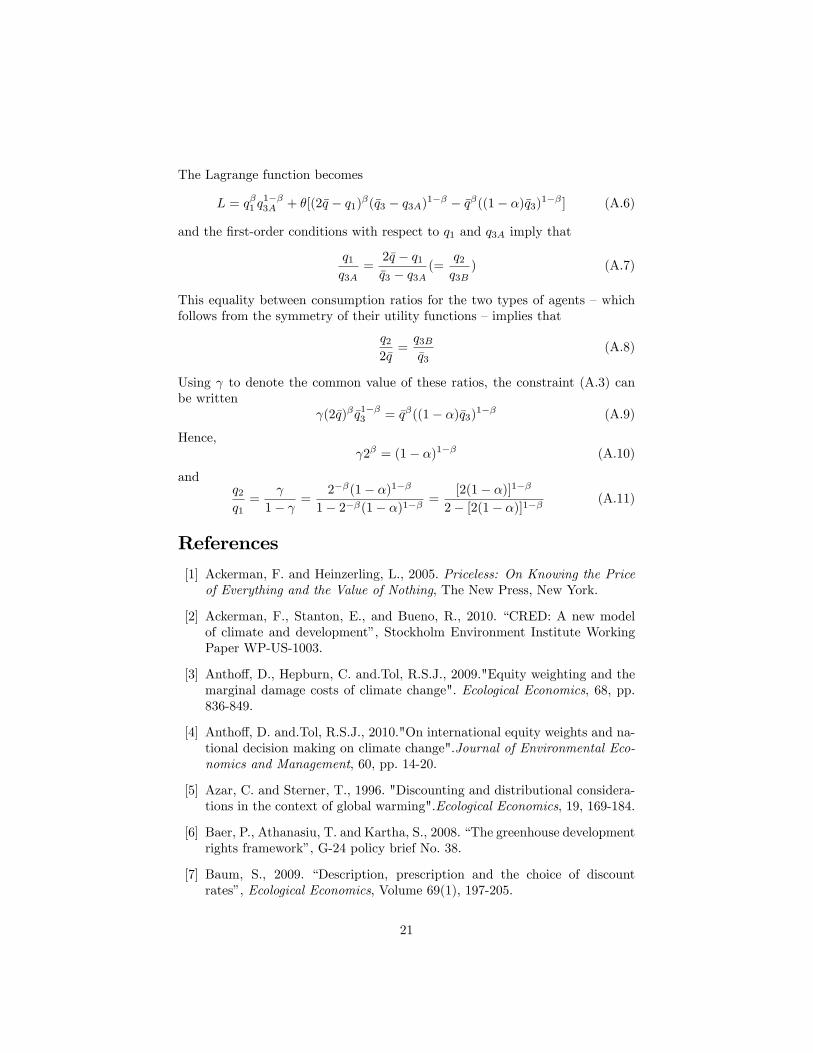
The Lagrange function becomes

L = q�1 q1��3A + �[(2�q � q1)�(�q3 � q3A)1�� � �q�((1� �)�q3)1�� ] (A.6)

and the �rst-order conditions with respect to q1 and q3A imply that

q1q3A

=2�q � q1�q3 � q3A

(=q2q3B

) (A.7)

This equality between consumption ratios for the two types of agents �whichfollows from the symmetry of their utility functions �implies that

q22�q=q3B�q3

(A.8)

Using to denote the common value of these ratios, the constraint (A.3) canbe written

(2�q)� �q1��3 = �q�((1� �)�q3)1�� (A.9)

Hence, 2� = (1� �)1�� (A.10)

andq2q1=

1� =2��(1� �)1��

1� 2��(1� �)1�� =[2(1� �)]1��

2� [2(1� �)]1�� (A.11)

References

[1] Ackerman, F. and Heinzerling, L., 2005. Priceless: On Knowing the Priceof Everything and the Value of Nothing, The New Press, New York.

[2] Ackerman, F., Stanton, E., and Bueno, R., 2010. �CRED: A new modelof climate and development�, Stockholm Environment Institute WorkingPaper WP-US-1003.

[3] Antho¤, D., Hepburn, C. and.Tol, R.S.J., 2009."Equity weighting and themarginal damage costs of climate change". Ecological Economics, 68, pp.836-849.

[4] Antho¤, D. and.Tol, R.S.J., 2010."On international equity weights and na-tional decision making on climate change".Journal of Environmental Eco-nomics and Management, 60, pp. 14-20.

[5] Azar, C. and Sterner, T., 1996. "Discounting and distributional considera-tions in the context of global warming".Ecological Economics, 19, 169-184.

[6] Baer, P., Athanasiu, T. and Kartha, S., 2008. �The greenhouse developmentrights framework�, G-24 policy brief No. 38.

[7] Baum, S., 2009. �Description, prescription and the choice of discountrates�, Ecological Economics, Volume 69(1), 197-205.

21

[8] Blanchard, O.J., 2008. �The state of macro�, NBER working paper 14259,http://www.nber.org/papers/w14259.

[9] Brenner, M., Riddle, M. and Boyce, J., 2007.�A Chinese sky trust? Distri-butional impacts of carbon charges and recycling in China�, Energy Policy,Volume 35(3), pp. 1771-1784.

[10] Chichilnisky, G., 1996.�An axiomatic approach to sustainable develop-ment�, Social Choice and Welfare, Volume 13, 231-257.

[11] Chichilnisky, G. and Heal, G., 1993. �Who should abate carbon emis-sions? An international viewpoint�, NBER Working paper 4425,http://www.nber.org/papers/w4425.

[12] Dasgupta, P., 2011. "The ethics of intergenerational distribution: reply andresponse to John E. Roemer". Environmental and Resource Economics, 50(4), 475-493.

[13] Davis, L. and Skott, P., 2012. �Positional goods, climate change and thesocial returns to investment�, forthcoming in a volume edited by A. Rezai,T. Michl and L. Taylor, Routledge.

[14] Debreu, G., 1974. �Excess demand functions�, Journal of MathematicalEconomics, Volume 1(1), 15-21.

[15] Hoel, M. and Sterner, T., 2007. �Discounting and relative prices�, ClimaticChange, Volume 84, 265-280.

[16] Intergovernmental Panel on Climate Change, 1996. �Climate Change 1995:Economic and Social Dimensions of Climate Change�, contribution ofWorking Group III to the Second Assessment Report of the Intergovern-mental Panel on Climate Change.

[17] Intergovernmental Panel on Climate Change, 2001. �Climate Change 2001:Impacts, Adaptation and Vulnerability: Summary for Policymakers�, ap-proved by Intergovernmental Panel on Climate Change Working Group IIin Geneva, 13-16 February.

[18] Kirman, A., 1992. �Who or what does the representative individual repre-sent?�The Journal of Economic Perspectives, Volume 6(2), 117-136.

[19] Mantel, R., 1976. �Homothetic preferences and community excess demandfunctions�, Journal of Economic Theory, Volume 12(2), 197-201.

[20] Narain, S. and Riddle, M., 2007. �Greenhouse justice: an entitlementframework for managing the global atmospheric commons�, in ReclaimingNature: Environmental Justice and Ecological Restoration, ed. J. Boyce, S.Narain, and E. Stanton. Anthem Press, London.

[21] Nordhaus, W.D., 1992. �An Optimal Transition Path for ControllingGreenhouse Gases�, Science, Volume 258, 1315-1319.

22

[22] Nordhaus, W.D., 1994.Managing the Global Commons: The Economics ofClimate Change. Cambridge, MA: MIT Press.

[23] Nordhaus, W.D., 2008. A Question of Balance: Weighing the Options onGlobal Warming, Yale University Press, New Haven.

[24] Nordhaus, W.D. and Boyer, J., 2000..Warming the World: Economic Mod-els of Global Warming, MIT Press, Cambridge.

[25] Rezai, A., Foley, D. and Taylor, L., 2011.�Global Warming and EconomicExternalities�, Economic Theory forthcoming (DOI 10.1007/s00199-010-0592-4)

[26] Roemer, J.E., 2011. "The ethics of distribution in a warming planet", En-vironmental and Resource Economics, 48(3), 363-390..

[27] Sen, A., 2000. �The discipline of cost-bene�t analysis�, The Journal ofLegal Studies, University of Chicago Press, Chicago.

[28] Sonnenschein, H., 1972. �Market excess demand functions�, Volume 40(3),549-563.

[29] Stanton, E., 2010.�Negishi welfare weights in integrated assessment models:the mathematics of global inequality�Climatic Change,

[30] Stern, N., 2006. The Economics of Climate Change: The Stern Review.Cambridge University Press, Cambridge. Online at http://www.hm-treasury.gov.uk/independent_reviews/stern_review_climate_change/sternreview_index.cfm.

[31] Stern, N., 2008. "The Economics of Climate Change". American EconomicReview: Papers & Proceedings, 98:2, 1�37

[32] Tol, R., 1995. �The damage costs of climate change�toward more compre-hensive calculations�, Environmental and Resource Economics, 5, 353-374.

[33] Tol, R., 2002. �Estimates of the damage costs of climate change - part II:dynamic estimates�. Environmental and Resource Economics, 21, 136-160.

[34] Weitzman, M.L., 2007."A Review of The Stern Review on the Economics ofClimate Change". Journal of Economic Literature, Vol. XLV (September),703�724.

[35] Weitzman, M.L., 2009. "On modeling and interpreting the economics ofcatastrophic climate change" Review of Economics and Statistics, 91(1),1-19.

[36] Woodford, M, 2003. Interest and Prices: Foundations of a Theory ofMonetary Policy. Princeton University Press, Princeton.

23