
Dissertation submitted to the Combined Faculties for the ...marin/temp/phd_sr.pdf · Prof. Dr....
136
Dissertation submitted to the Combined Faculties for the Natural Sciences and for Mathematics of the Ruperto-Carola University of Heidelberg, Germany for the degree of Doctor of Natural Sciences presented by Dipl-Phys. Rachik Soualah born in Biskra, Algeria Oral examination: ..th April, 2009
Transcript of Dissertation submitted to the Combined Faculties for the ...marin/temp/phd_sr.pdf · Prof. Dr....

Dissertationsubmitted to the
Combined Faculties for the Natural Sciences and for Mathematicsof the Ruperto-Carola University of Heidelberg, Germany
for the degree ofDoctor of Natural Sciences
presented by
Dipl-Phys. Rachik Soualahborn in Biskra, Algeria
Oral examination: ..th April, 2009


Production of Neutral Pions in Pb+Au collisionsat 158 AGeV/c
Referees: Prof. Dr. Johanna StachelProf. Dr. Norbert Herrmann


Abstract in English
Abstrac in german


Contents
Overview 1
1 Introduction 1
1.1 The Standard Model . . . . . . . . . . . . . . . . . . . . . . . 1
1.2 The Strong interactions . . . . . . . . . . . . . . . . . . . . . . 3
1.2.1 The QCD Lagrangian . . . . . . . . . . . . . . . . . . . 3
1.2.2 Asymptotic freedom . . . . . . . . . . . . . . . . . . . 4
1.2.3 The quarks confinement . . . . . . . . . . . . . . . . . 5
1.2.4 Deconfinement and the Quark Gluon Plasma . . . . . . 7
1.2.5 The Lattice QCD . . . . . . . . . . . . . . . . . . . . 9
1.3 The ultra relativistic heavy ion collisions . . . . . . . . . . . . 10
1.3.1 Machines . . . . . . . . . . . . . . . . . . . . . . . . . 10
1.3.2 The Geometry of the collision . . . . . . . . . . . . . . 10
1.3.3 The evolution of the QGP: Scenario of Bjorken . . . . 12
1.3.4 The experimental observations of the QGP . . . . . . . 14
2 The CERES Experiment 19
2.1 Experimental setup overview . . . . . . . . . . . . . . . . . . . 19
2.2 The target region . . . . . . . . . . . . . . . . . . . . . . . . . 21
2.3 The trigger system . . . . . . . . . . . . . . . . . . . . . . . . 22
2.4 The Silicon Drift Detectors . . . . . . . . . . . . . . . . . . . . 23
2.5 The RICH Detectors . . . . . . . . . . . . . . . . . . . . . . . 25
2.6 The Time Projection Chamber (TPC) . . . . . . . . . . . . . 27
2.7 The CERES Time Projection Chamber . . . . . . . . . . . . 28
2.7.1 The geometry . . . . . . . . . . . . . . . . . . . . . . . 28
2.7.2 The coordinate system . . . . . . . . . . . . . . . . . . 28
2.7.3 The read-out system: principle of operation . . . . . . 29
2.7.4 TPC track reconstruction . . . . . . . . . . . . . . . . 32
2.7.5 TPC Track fitting . . . . . . . . . . . . . . . . . . . . . 36
2.7.6 Particle identification using dE/dx measurement . . . . 39
I

3 The Data Analysis 413.0.7 Event data base . . . . . . . . . . . . . . . . . . . . . . 41
3.1 The reconstruction chain . . . . . . . . . . . . . . . . . . . . . 423.2 The Electron and Positron selection . . . . . . . . . . . . . . . 433.3 The mixing event method . . . . . . . . . . . . . . . . . . . . 443.4 The standard Quality cut . . . . . . . . . . . . . . . . . . . . 473.5 The study of the unlike and like sign pairs . . . . . . . . . . . 483.6 The photon reconstruction . . . . . . . . . . . . . . . . . . . . 53
3.6.1 Photon-Matter interaction . . . . . . . . . . . . . . . . 533.6.2 Photon conversions (γZ −→ e+e−Z) . . . . . . . . . . 543.6.3 The reconstructed photon mapping . . . . . . . . . . . 55
3.7 The Secondary vertex fit algorithme . . . . . . . . . . . . . . . 563.7.1 The mathematics of the Secondary Vertex fit . . . . . . 583.7.2 Application of the Secondary vertex method . . . . . . 633.7.3 Secondary vertex cut (SV) . . . . . . . . . . . . . . . 65
3.8 The π0 reconstrcution . . . . . . . . . . . . . . . . . . . . . . 703.8.1 Invariant mass analysis . . . . . . . . . . . . . . . . . . 70
4 Monte Carlo Simulations 874.1 Introduction . . . . . . . . . . . . . . . . . . . . . . . . . . . . 874.2 The Event Generator . . . . . . . . . . . . . . . . . . . . . . . 88
4.2.1 Expected number of π0 mesons . . . . . . . . . . . . . 904.3 The detector simulation . . . . . . . . . . . . . . . . . . . . . 93
4.3.1 The Conversion from Step2 to Step3c . . . . . . . . . . 944.3.2 The reconstructed tracks Comparison . . . . . . . . . . 94
4.4 The unlike/like sign pairs comparison . . . . . . . . . . . . . . 984.5 The Photon mapping comparison . . . . . . . . . . . . . . . . 1004.6 The Secondary Vertex Comparison . . . . . . . . . . . . . . . 1004.7 The γγ invariant mass distributions . . . . . . . . . . . . . . . 1014.8 Acceptance and efficiency evaluation . . . . . . . . . . . . . . 102
Bibliography 119
II

List of Figures
1.1 The αQCD coupling constant . . . . . . . . . . . . . . . . . . . 61.2 The quark-antiquark potential . . . . . . . . . . . . . . . . . . 71.3 The phase transition diagram of hadronic matter . . . . . . . 81.4 The lattice QCD . . . . . . . . . . . . . . . . . . . . . . . . . 91.5 The geometry of collision . . . . . . . . . . . . . . . . . . . . . 111.6 The geometry of collision . . . . . . . . . . . . . . . . . . . . . 131.7 Feynmann diagram . . . . . . . . . . . . . . . . . . . . . . . . 15
2.1 The CERES experimental setup. . . . . . . . . . . . . . . . . 202.2 The Target area: 1 - The vacuum pipe, 2 - The entrance win-
dow, 3 - BC2 4 - BC2’s PMT, 5 - Au target, 6 - BC3’s PMT, 7- MC’s PMT, 8 - BC3, 9 - MC scintillator, 10 - Al-mylar lightguide, 11 - SiDC1(down), 11 - SiDC2(up), 13 - Gas radiator. . 21
2.3 Schematic view of trigger detectors. . . . . . . . . . . . . . . . 222.4 Working mode of the Silicon Detectors. . . . . . . . . . . . . 232.5 A central Pb− Au event in the SiDC detector. . . . . . . . . . 242.6 The SDD anode structure. . . . . . . . . . . . . . . . . . . . 252.7 The Principle operation of the CERES RICH detector . . . . . 262.8 Perspective view of the CERES Time Projection Chamber. . . 292.9 The TPC coordinate system. . . . . . . . . . . . . . . . . . . . 302.10 The electric potential map of the CERES TPC radout cham-
bers simulated with the GARFIELD package. . . . . . . . . . 312.11 Cross section of the TPC readout chambers. . . . . . . . . . . 322.12 Four single cheveron pads of the cathode pads compose one
readout chamber. . . . . . . . . . . . . . . . . . . . . . . . . . 332.13 The magnetic field in the CERES TPC. . . . . . . . . . . . . 332.14 Schematic event display of the TPC. . . . . . . . . . . . . . . 342.15 The TPC hit finding procedure. . . . . . . . . . . . . . . . . . 352.16 The TPC overlapping hit reconstruction. The absolute max-
imum of the considered hit is stored by the counter variable.It will be increases by the the absolute maxima of the overlap-ping neighbors whenever a founded pixel is shared to severalhits. . . . . . . . . . . . . . . . . . . . . . . . . . . . . . . . . 36
III

2.17 The momentum resolution obtained from a Monte Carlo simu-lation of the detector,the blue points used for the 3-parameterfit, the red for the 2-parameter fit and black for the combinedmomentum fit. . . . . . . . . . . . . . . . . . . . . . . . . . . 38
2.18 The energy loss of charged particles as a function of their mo-mentum.The lines indicate the predicted dE/dx areas by theBethe-Bloch formula for π, K, ρ, d and e . . . . . . . . . . . . 39
3.1 The energy loss of the charged partilces. . . . . . . . . . . . . 433.2 The multiplicities of electrons and positrons in each event.
The selection was obtained by using the energy loss informa-tion. provided from TPC detector. . . . . . . . . . . . . . . . 45
3.3 Mixing event Method . . . . . . . . . . . . . . . . . . . . . . . 463.4 The used track quality criteria . . . . . . . . . . . . . . . . . . 473.5 The distribution of the number of the TPC fitted hits . . . . . 483.6 The variation of the opening angle between the unlike sign
e+e− (blue line) and the like signs . . . . . . . . . . . . . . . . 503.7 The ratio of the unlike sign e+e− and the like signs e+e+, e−e−
Vs the opening angle . . . . . . . . . . . . . . . . . . . . . . . 523.9 The number of the reconstructed electrons and positrons in
each event by using the dEdx information provided from TPCdetector. . . . . . . . . . . . . . . . . . . . . . . . . . . . . . . 55
3.10 Schematic event display of the TPC. . . . . . . . . . . . . . . 563.11 The Gamma mapping of the reconstructed photons . . . . . . 573.12 ... . . . . . . . . . . . . . . . . . . . . . . . . . . . . . . . . . . 633.13 The Secondary Vertex distributions of the photons condidates.
The reconstructed photons from the unlike sign pairs (e−e+)are in bleu and the like sign pairs.(e−e− + (e−e+)) in red. Thetop two plots correspond to Secondary Vertex distributionson the X axis before and after the ThetaEP cut while on thebottom two plots, the same distributions on the Y axis beforeand after the ThetaEP cut . . . . . . . . . . . . . . . . . . . . 65
3.14 The projection of the Secondary Vertex distribution on theX-Y plane.The most populated area indicates the positions ofthe reconstructed photons. . . . . . . . . . . . . . . . . . . . . 66
3.15 The Z direction of the Secondary Vertex distributions of thephoton condidates before (left) and after (right) imposing theThetaEP cut. . . . . . . . . . . . . . . . . . . . . . . . . . . . 67
3.16 The measured Z direction of the Secondary Vertex distribu-tions after the ThetaEP cut as function of the photon momen-tum. . . . . . . . . . . . . . . . . . . . . . . . . . . . . . . . . 68
IV

3.17 The extracted signal distribution of the converted photons Vsthe momentum of the photon. . . . . . . . . . . . . . . . . . . 69
3.18 The mean and the width of the fitted Seondary vertex distri-bution Vs the phton momentum. . . . . . . . . . . . . . . . . 70
3.19 The mean and the width of the fitted Seondary vertex distri-bution Vs the phton momentum. . . . . . . . . . . . . . . . . 71
3.20 The scatter plot of the π0 transeverse momenta vs the openingangle between the two photons. The OpG1G2 cut is indicatedby the maginta line. . . . . . . . . . . . . . . . . . . . . . . . . 73
3.21 The invariant mass distribution for all the photons comingfrom the same event(blue histogram) and the mixing event(red histogram) for the rapidity range 2.2 ≤ y < 2.4 and 8 pt
bins of 0.25GeV . . . . . . . . . . . . . . . . . . . . . . . . . 743.22 The invariant mass distribution for all the photons coming
from the same event(blue histogram) and the mixing event(red histogram) for the rapidity range 2.4 ≤ y < 2.6 and 8 pt
bins of 0.25GeV . . . . . . . . . . . . . . . . . . . . . . . . . 753.23 The invariant mass distribution for all the photons coming
from the same event(blue histogram) and the mixing event(red histogram) for the rapidity range 2.4 ≤ y < 2.7 and 8 pt
bins of 0.25GeV . . . . . . . . . . . . . . . . . . . . . . . . . 763.24 The ratio of the same and mixed events mass distributions for
the rapidity range 2.2 ≤ y < 2.4 and 8 pt bins of 0.25GeV . . 773.25 The ratio of the same and mixed events mass distributions for
the rapidity range 2.4 ≤ y < 2.6 and 8 pt bins of 0.25GeV . . . 783.26 The ratio of the same and mixed events mass distributions for
the rapidity range 2.6 ≤ y < 2.7 and 8 pt bins of 0.25GeV . . 793.27 The mean and the width of the fitted Seondary vertex distri-
bution Vs the phton momentum. . . . . . . . . . . . . . . . . 803.28 The real mass distribuion of π0 after subtracting the normal-
ized mixed event distribution in the range 2.2 < y < 2.4 and8 pt bins of 0.25GeV . . . . . . . . . . . . . . . . . . . . . . . 82
3.29 The real mass distribuion of π0 after subtracting the normal-ized mixed event distribution in the range 2.2 < y < 2.4 and8 pt bins of 0.25GeV . . . . . . . . . . . . . . . . . . . . . . . 83
3.30 The real mass distribuion of π0 after subtracting the normal-ized mixed event distribution in the range 2.2 < y < 2.4 and8 pt bins of 0.25GeV . . . . . . . . . . . . . . . . . . . . . . . 84
4.1 The mT spectra inverse slopes T on the particle mass m atCERN-SPS Pb-Pb collisions . . . . . . . . . . . . . . . . . . . 89
V

4.2 The distribution of the neutral pion rapidity versus the trans-verse momentum. . . . . . . . . . . . . . . . . . . . . . . . . . 90
4.3 The (γγ) opening angle distribution versus the transverse mo-mentum of the neutral pion . . . . . . . . . . . . . . . . . . . 91
4.4 The comparison between the Thermal model and the experi-mental data particle ratios. . . . . . . . . . . . . . . . . . . . . 92
4.5 The The Purity distribution of the reconstructed charged tracksfrom the Overlay Monte Carlo . . . . . . . . . . . . . . . . . . 95
4.6 The polar and the azimuthal angles distributions from thereconstructed tracks and the simulated tracks . . . . . . . . . 96
4.7 The TPC reconstruction efficiencies as function of the polarand the azimuthal angles. . . . . . . . . . . . . . . . . . . . . 97
4.8 The comparison of the TPC number of fitted hits on the trackfor Overlay Monte Carlo simulation and for data . . . . . . . 97
4.9 The Photon signal distribution comparison between the Over-lay Monte Carlo and data . . . . . . . . . . . . . . . . . . . . 104
4.10 The tighter energy loss cut cross checking of the bumps in thephoton signal at high momentum . . . . . . . . . . . . . . . . 105
4.11 The Photon signal distribution comparison between the Over-lay Monte Carlo and data after the new dEdx condition . . . 106
4.12 The Mean and Width of the Secondary vertex. . . . . . . . . . 1074.13 The Mean and Width of the Secondary vertex. . . . . . . . . . 1084.14 The Secondary Vertex distributions of the subtracted signal to
backround reconstructed in the Overly Monte Carlo simulations.1094.15 The position and the width of the photon vertex converting
to e−e+ for Overly Monte Carlo and data. . . . . . . . . . . . 1104.16 The Mean and Width of the Secondary vertex. . . . . . . . . . 1114.17 The Mean and Width of the Secondary vertex. . . . . . . . . . 1124.18 The Mean and Width of the Secondary vertex. . . . . . . . . . 1134.19 The Mean and Width of the Secondary vertex. . . . . . . . . . 1144.20 The Mean and Width of the Secondary vertex. . . . . . . . . . 1154.21 The acceptance of the neutral pion as function of rapidity and
transverse momentum. . . . . . . . . . . . . . . . . . . . . . . 1164.22 The reconstruction efficiencies distributions versus the π0 trans-
verse momentum . . . . . . . . . . . . . . . . . . . . . . . . . 117
VI

List of Tables
1.1 Number of events and beam particles for all targets . . . . . . 11
VII


In any subject which has principles, causes,and elements, scientific knowledge and un-derstanding stems from a grasp of these,for we think we know a thing only when wehave grasped its first causes and principlesand have traced it back to its elements
Aristotle, Physics
1Introduction
1.1 The Standard Model
The laws of physics governing the world of elementary particles are now verywell described by what we call the Standard Model of particle physics fruitof major theoretical and experimental advances of the twentieth century. Todescribe and understand Nature, physicists have worked to determine thebasic constituents (elementary particles) which it is made and to define theinteractions that govern theirs fundamental interactions.In nature there are 12 matter particles and the 4 particles interactions ofthe standard model. It also provides that for every particle there is an anti-particle same mass but an opposed charge and parity. All these buildingblocks are grouped into three families growing masses. The stable matterparticles composed of the first family whose members are the lightest.Today, physics is understood through a series of elementary particles, whichare classified into two main families: the fermions.1 (particles of half-integerspin) and bosons (integer spin). The fermions follow the Pauli ExclusionPrinciple and they are the constituent particles of the ordinary matter-theproton, neutron and electron belong to this family. The bosons are theparticles carrying the information exchanged between fermions during an in-teraction.Among the fermions, six of them are classified as quarks (up, down, charm,strange, top, bottom), and the other six as leptons (electron, muon, tau,
1is a particle of half integer spin.
1

2 CHAPTER 1. INTRODUCTION
and their corresponding neutrinos). The quarks do not feel the strong inter-action, and leptons are insensitive to it. Leptons are directly observable innature. Quarks, however, are not directly observed in that they do not ap-pear to exist by themselves as free particles. We can model each fundamentalinteraction between elementary particles by the exchange of bosons, namelyparticles integer spin, obeying the Bose-Einstein statistics which allows themto accumulate in the same condition. These particles ”carry” the interactionof a particle to another and are thus called vector bosons. Four interactionshave been identified:Electromagnetic interaction where the photon is the intermediate vector bo-son. The photon does not have itself an electric charge, it is neutral, andparticles exchanging photons retain their electric charge unchanged after theexchange. The mass of the photon is zero; the electromagnetic interactionlength is infinite.The weak interaction with three vector bosons: Z0, electrically neutral, andW± have an electric charge ±1. It deals with all fermions through twocharges, where one of these two charges is laid by the left handed fermions.The strong interaction, the gauge bosons are the gluons and they form anoctet. Among the fermions, only quarks have a known color, which may takethree values appointed by agreement ”red”, ”green” and ”blue”. The gluonsalso have this feature, a combination of colors and anti-colors, and can thuscombine them. They have zero mass.The standard model thus encompasses all known particles and the three inter-actions with a wide effect of the particle. This is done through the quantumfield theory that constitutes the mathematical framework of the model. Thestandard model allows us to explain all natural phenomena except gravity,which is for the moment, resists the theorists for a quantum theory andwhich can be neglected during the interaction between elementary particles,because of the weakness of the gravitational intensity force compared to theprevious forces.The structure of each interactions included in the Standard Model is dictatedby the group of symmetry which leaves the action invariant. The model in-troduces the group symmetry gauge following:
SU(2)L ⊗ U(1)Y ⊗ SU(3)C (1.1)
The SU(2)L ⊗U(1)Y gauge group combined both the electromagnetism andweak interaction theories into a single unified theory of electroweak theoryof Glashow-Weinberg-Salam with the gauge group. It contains four quantaof radiation, one for the U(1) part and three for SU(2). The term SU(3)C isthe color gauge group which describes the strong interactions. The Gluonsare its 8 quanta of radiation.

1.2. THE STRONG INTERACTIONS 3
1.2 The Strong interactions
The Quantum ChromoDynamique (QCD) is the general accepted gauge the-ory [1, 2] used to reflect the strong interactions [4, 5] between basic con-stituents of nuclear matter. This approach to standard model is certainlyits most complicated component insofar as its Lagrangian uses only quarksand gluons to describe the confined states (hadrons). Quarks do not interactwith each other directly; they do so through the gluons as intermediatedagents. We can only refer to there presence in objects which are color sin-glets. A colored quark can be bound with an antiquark with correspondinganticolor to form a meson. Three quarks of different colors can be boundto form baryon. Mesons and baryons are collectively called hadrons to bedistinguished from the leptons and filed bosons as the ”particles” which canbe directly measured.
1.2.1 The QCD Lagrangian
The QCD is a Yang-Mills theory of colored quarks and gluons introduced byGell-Mann [9] and Zweig[10] in the 60’s. It required the introduction of a newhidden quantum number in order to do not violate the Fermi Statistics for theparticle ∆++(uuu): color. All baryons (set of three quarks) and all mesons(pair of quark-antiquark) are singlets colors. Theirs symmetry properties aredescribed by the SU(3)c. We can define a local transformation gauge as theform:
U = exp(g3
∑a
αa(x)Ta), a = 1, 8 (1.2)
here the g3 is the QCD coupling constant, the matrices Ta represent the gen-erators of the SU(3)c gauge group and αa are an arbitrary phases dependenton the space-time coordinates. The QCD Lagrangian involve a bosonic partand fermionic part, it takes the following form:
LQCD =1
4F a
µνFµνa +
6∑q=1
(iψqγµDµψq −mqψqψq) (1.3)
With the field strength tensor:
F aµν = ∂µA
aν − ∂νA
aµ + gsfabcA
bνA
cµ (1.4)
and the covariant derivative:
Dµ = ∂µ + igsλa
2Aa
µ (1.5)

4 CHAPTER 1. INTRODUCTION
The last term in Eq.(1.4) contain the fundamental difference between QEDand QCD which describes the self coupling of gluons. This approach al-lows interaction between gluons giving rise to the definition of a vertex 3 or4 gluons while in QED, the interaction between photons is not permitted.The The six quarks q are represented by the spinors ψq which are the 4-component Dirac spinors associated with each quark field of (3) color i andflavor q, the Aa
ν are the (8) Yang-Mills (gluon) fields as well as the associatedcovariant derivatives Dµ and fabc are the structure constants of the SU(3)algebra. The very limited length scale of the strong interaction, of the orderof 10−15 meters, is due to the gauge bosons self-coupling. This also par-ticularly implies that the interaction strength between two quarks increaseswith their relative distance. The interaction between quarks grows weakeras the quarks approach one another more closely. This important propertiesof the strong interaction and its physics can be divided into two regimes:asymptotic freedom and confinement [12].
1.2.2 Asymptotic freedom
One of the striking properties of QCD is asymptotic freedom which statesthat the interaction strength between quarks becomes smaller as the distancebetween them gets shorter so that quarks behave almost as free particles.Similarly to the QED, the coupling constant of QCD is defined by
αs =gs
2π~c(1.6)
The αs value shows a strong dependence on the momentum transfer Q2 in acollision. The αs(Q
2) evolution is governed by theory through the differentialequation of renormalization group[2]:
Q2 ∂αs
∂Q2= β(αs) (1.7)
If we consider only the first order of αs, the function is calculated by aperturbative treatment of QCD as a development of the strong coupling:
βαs = −bα2s(1 + ϑ(α3
s))withb =33− 2nf
12π(1.8)
For the leading order perturbative approximation the solution of this equa-tion gives the variation of the coupling constant to the scale of the momentumtransfer at large momentum:
αs(Q2) =
α0
1 + α033−2nf
12πln −Q2
µ2
(1.9)

1.2. THE STRONG INTERACTIONS 5
Where α0 is the coupling constant for nf number of active quark flavors withthe momentum transfer µ.
From equation (..) we conclude that for a number of flavors less than 17,the coupling constant decreasing slowly to zero when Q2 >> µ2,i.e. preciselywhere the asymptotic freedom is. Therefore the quarks behave as they werefree inside the hadrons. At this stage when the momentum transfer is large,the strong interaction physics can be calculated in perturbative theory. Thevariation of the coupling constant diverges for small values of Q2 < µ2 bearthe application of perturbative treatment to calculate the physical observableinaccurate. In this prevailing order a new phenomenon, coming directly fromthe non-abelian propriety of the theory. The Fig. 1.1 illustrate the decreas-ing of the strong interaction constant coupling depending on the momentumtransfer. The QCD is therefore perturbative and calculable at short distance(large Q): the asymptotic freedom. However, long-distance (low Q), the cou-pling constant becomes too big and the perturbatif calculations are no longervalid. Another approach can be done, in order to estimate the evolution ofthe coupling constant by introducing directly in the definition of the couplinga new parameter λQCD which sets the scale at which the coupling constantbecomes large and the physics becomes nonperturbative. The ΛQCD valuecan be determined experimentally and it is on the order of 200 MeV:
αs(Q2) =
1
(33−2nf
12π) ln( Q
ΛQCD)2
(1.10)
It remains to solve the problem of formulating the QCD theory in a non-perturbatif when the strong interaction coupling becomes hard for large dis-tances between quarks (upper than fm) or for small energy scale energy (lessthan GeV ). A solution is provided by the Lattice QCD method.
1.2.3 The quarks confinement
One of the prominent prosperities of QCD is the formation of color singletobjects. This feature is called the color confinement of quarks in hadrons. Inthe same way as the electric charges of the opposite sign attraction, the colorcharge attracts quarks with different colors. The QCD explains,in particu-lar, the formation of hadrons. When the quarks moves away from each other(the energy put into play decreases), more gluons are exchanged. These glu-ons themselves can interact with each other or a couple of new pairs virtualquark-antiquark. Beyond a typical distance of 1fm (10−15m), quarks canno longer spread freely and remain confined within hadrons. This phase ofhadronization taken over the non-perturbative QCD regime is generally de-scribed by phenomenological models. In general, if the potential between two

6 CHAPTER 1. INTRODUCTION
QCDO(α )
245 MeV
181 MeV
ΛMS(5) α (Μ )s Z
0.1210
0.1156
0.1
0.2
0.3
0.4
0.5
αs(Q)
1 10 100Q [GeV]
Heavy QuarkoniaHadron Collisionse+e- AnnihilationDeep Inelastic Scattering
NL
O
NN
LO
TheoryData L
attic
e
211 MeV 0.1183s4 {
Figure 1.1: The αQCD coupling constant [6].
quarks is proportional to the distance between them, then the two quarks cannever be separated. To illustrate this character, a classic parameterization[7, 8, 9] of potential inter-quarks is proposed in the equation:
V (r) = V0 − π
12.1
r+ σ.r (1.11)
The second term of this equation shows the Colombian interaction for shortdistances, the confinement is represented by the last term where σ is calledthe string tension. One may try to separate the quarks by pulling them apart,then the restoring force of the linear potential between them grows sufficientlyrapidly to prevent them from being separated. The interaction between thequarks gets stronger as the distance between them gets larger. The form ofthe potential results of these two terms is shown in Figure 1.1 depending onthe separation distance r. The potential between the two quarks becomeslinear and is growing to infinity with the inter-quarks distance.
Figure du potential quark anti-quark.

1.2. THE STRONG INTERACTIONS 7
0 1 2 3 4 5 6 7 8 9r
0
0,2
0,4
0,6
0,8
1
1,2V
(r)
Figure 1.2: The potential between two quarks as function of the distance.
1.2.4 Deconfinement and the Quark Gluon Plasma
It is believed that the universe consisted of quark and gluons transforming tohadronic matter just a few microseconds after the Big Bang. Theories alsopredict that it may still exist in the universe that we see today since the coresof dense neutron stars and the supernova supply extreme astrophysical envi-ronments which favor the creation and the existence of this state. Among thegoals of current nuclear researches is the observation of this new undiscoveredstate called Quark Gluon Plasma (QGP) [10] in which its building blocks(quarks and gluons) act in like free particles. The search for a such phasetransition from the confined hadronic matter to the deconfined QGP matteris a fascinating subject to study the dynamics of this interface. The natureof the strong interaction has been described as in the case of the hadronsordinary matter. However, it is crucial to be able to describe the behavior ofthe matter under conditions of temperature and density, particularly whenone or both of these two quantities are extremely high.The challenge is to understand the substance of the Universe during its firstmoments, but also of existing forms such as inside the compact stars formedby the gravitational collapse of the supernovae nucleus. We can talk aboutphase transition when certain properties of nuclear matter undergo a radi-cal change for that reason the system can be well described using statisticalmechanics description which provides global variables and other conservedquantities. The grand canonical ensemble is therefore used to describe thewhole system allowing the variation of the particles number. The parametersof the control are then the temperature T , the volume V and the chemical

8 CHAPTER 1. INTRODUCTION
potential µ. The latter represents the necessary energy to provide to thesystem in order to add a quark. Generally the diagram of phases dependingon the temperature (T ) and potential chemical baryonic, as shown in Figure:By increasing T or µb, a phase transition is possible to occur. The evolution
0
25
50
75
100
125
150
175
200
225
0 200 400 600 800 1000 1200
µb (MeV)
T (
MeV
)
dN/dy 4πData (fits)
LQCDQGP
hadrons
crossover1st order
critical point
nb=0.12 fm-3hadron gas
ε=500 MeV/fm3
Figure 1.3: The phase transition diagram of hadronic matter [11].
of the universe can be traced from its earliest moments, where the temper-ature was well above Tc and at low chemical potential. The bottom left ofthis diagram correspond to a low temperature and low potential baryonic,the behavior of QCD thermodynamics can be described in terms of hadrongas (states composed of related quarks and gluons): If we increase the tem-perature of the system, this state can not exist as it is. There is a smallarea where this matter is undergoing a transition considered as cross over,from which the degrees of freedom are not the hadrons but quarks and gluonsthemselves. The high µ and small T on the right of the diagram, correspondsto a region accessible by compressing the system. This state of matter is amatter of quarks that can be found in the hearts of neutron stars [12].

1.2. THE STRONG INTERACTIONS 9
1.2.5 The Lattice QCD
The estimations of the preceding paragraph are based on very rough approx-imations. At large distances (i.e. small scales); it becomes impossible to usethe perturbative theory to achieve results. Indeed, the interactions betweenquarks and gluons are too strong and perturbative approach can not work.In particular, the QGP can not really be considered as gas particles withoutinteraction. To take in account these interactions we should use the QCD tomodel all the interactions existing in the system. In this framework, Latticesimulations of QCD thermodynamics have made significant progress in thelast decade. The method of Lattice QCD allows a statistical approach ofthe strong interaction for complex systems. It gives access to the thermody-namic characteristics of a quarks and gluons system at the equilibrium. Therapid rise in computational power and implementation of better algorithmsauthorize the simulation of the behavior of matter by the QCD equations,which describes the strong interaction suffered by the quarks and gluons.The whole technic is based on the discretization of space-time on the finitedomain. The particles involved in the simulation are located on the nodesof the Lattice. An introduction to the used lattice QCD methods and itstechnical details could be founded in [13].
0.0
2.0
4.0
6.0
8.0
10.0
12.0
14.0
16.0
1.0 1.5 2.0 2.5 3.0 3.5 4.0
T/Tc
ε/T4 εSB/T4
3 flavour2+1 flavour
2 flavour
0
1
2
3
4
5
100 200 300 400 500 600
T [MeV]
p/T4 pSB/T4
3 flavour2+1 flavour
2 flavourpure gauge
Figure 1.4: The lattice QCD [14].
Initially, the developments were limited to µb = 0 and they can calculatethe evolution of pressure depending on the temperature. Figure 1 showsthe evolution predictions of the energy density (left) and pressure (right)depending on the temperature. This method of studying deconfinement takeinto account 3 assumptions: two light quark (u and d), three light quarks (u,d or s), or two light flavors (u and d) and a heavy flavor(s). A transition fromthe hadronic phase to partonic phase is clearly visible. The energy densityundergoes a rapid change near a critical temperature TC, enhanced by almost

10 CHAPTER 1. INTRODUCTION
an order of magnitude, as indicated in Figure 1. The temperature Tc dependson the number of flavors (nf) considered: Tc = 175 MeV for two light quarks(2 flavors), Tc = 155MeV for three light quark (3 flavors)[flavours]. Thereported error is the statistical error only and therefore it does not takeinto account the engendered systematical error by the discretization of thelattice. The Lattice QCD confirms the sharp increase, already estimated bythe equations 8 and 10, of the number of degrees of freedom of the system tothe temperature of the phase transition. This rapid change is an indicationthat the fundamental degrees of freedom are different above and below thecritical temperature.
1.3 The ultra relativistic heavy ion collisions
1.3.1 Machines
The goal of research in the ultra relativistic heavy ions is studying the pos-sible formation of a new state of nuclear matter called Quark and GluonPlasma (QGP). It is believed that this state of matter can be reached at ul-tra relativistic heavy ions collisions with targets to achieve sufficient energydensity and temperature. Under these circumstances, the nuclear materialundergoes a deconfined phase transition leading to the formation of the QGP.To simulate such extreme conditions here on earth, Ultra relativistic heavyion collisions between two nuclei were performed and an experimental cam-paign has therefore launched since 1986 to prove its existence and to studyit. The program of this campaign used to study the dense matter. Thedifferent used machines for this subject are presented in Table 1: the Alter-nating Gradiant Synchrotron (AGS)and the Relativistic Heavy Ion Collider(RHIC) at the Brookhaven National Laboratory (BNL) and the Super Pro-ton Synchrotron (SPS) , the future Linear Hadron Collider(LHC)at CERN.The main objective of these accelerators (red circles in Fig) is to draw adetailed description for the path of the universe in the opposite direction byraising the temperature in the area where the nuclei are collided.
1.3.2 The Geometry of the collision
A nucleus-nucleus collision at very high energy produces a large number ofhadrons near the center of mass. The attained energy density during thecollision depends on the energy of the incident nucleus,their longitudinal size(atomic mass) and the fireball volume that is big enough to explore theQGP. The corresponding Lorentz contraction is important since it is already

1.3. THE ULTRA RELATIVISTIC HEAVY ION COLLISIONS 11
Name Mode Beam E (AGeV )√
(SNN) (GeV ) ε(GeV/fm3)SIS fixed
targetU238 1 1.4
AGS fixedtarget
Pb208 12 4.9 1.0
SPS fixedtarget
Pb208 158 17.3 2.5
RHIC collider Au197 100 200 5LHC collider Pb208 2750 550 10
Table 1.1: Number of events and beam particles before and after cutting on thetime of the start counter and the vertex vz of the CDC.
γ1 = 10 for the SPS and it make also sure that the deformation is in thedirection of movement. The centrality of the collision or the recovery degreeof two nuclei at the collision time is usually given as a percentage of the totalcross section. We might define then from these measurements an importantvariable at this stage: the impact parameter b, which gives the distancebetween the axes of the two nucleuses. This description can be illustratedby figures 1.
b
Nucleus A Nucleus A
b
Nucleus B Nucleus B
(b) (a)
Figure 1.5: The geometry.
Here we describe the case of the most central collisions as they permitto get the higher energy density and they are essentially in the form of ahadrons gas. When a collision occurs at low impact parameter b, the mea-sured number of particles will be big, and the collision will be central. In

12 CHAPTER 1. INTRODUCTION
contrast, a collision at high impact parameter is peripheral. One can under-line the principal observables which characterize the dynamic of the collisionthat are expressed in term of rapidity:
y =1
2lnE + pL
E − pL
(1.12)
where E is the total energy of the particle and PL is its longitudinal momen-tum. When the energy density is important to the mass of the particle, weprefer to use the pseudo-rapidity variable:
η =1
2ln|p|+ pL
|p| − pL
= − ln(tan θ0) (1.13)
where θ is the angle between the particle momentum and the beam axis. Theenergy density initial EBj produced in the collisions can then be calculatedusing the formula 1 [Bjorken 1]: (write the one in the paper draft)
EBj =1
AT τ0.dEt
dy(1.14)
This equation takes into account the overlapping transverse surface betweenthe nucleons AT (depends on B), T0 the proper time of the partons ther-malisation (estimated at around 1fm/c) and the measurement of the totaltransverse energy, for such particle i emitted by an angle θi, is defined by:
ET =∑i=1
Ei. sin(θ) (1.15)
The energy densities at CERN-SPS energy is on the average of 3.9GeV/fm3
From the equation 1 we conclude also that the more energy density is highthe more we have the possibility to create the QGP.
1.3.3 The evolution of the QGP: Scenario of Bjorken
To reach the Quark-Gluons Plasma, extreme scenarios must be re-createdby colliding heavy ions with velocities close to the speed of light: enormoustemperatures, pressure and densities of those first few microseconds. Theframework of the space-time evolution of ultra-relativistic heavy ion collisionsis defined qualitatively and even quantitatively in terms of the reached energydensity. This scenario of evolution was proposed by Bjorken in 1983 [Bjorken2] and is represented in Figure 1.
The system presents a succession of several phases. In the pre-equilibriumphase, about typical time of T0 of 1fm/c, the system is thermalised and led

1.3. THE ULTRA RELATIVISTIC HEAVY ION COLLISIONS 13
Figure 1.6: The evolution of the Quark Gluon Plasma.
to the formation of QGP in total lifetime of the order of 5 to 7fm/c. Thequark-gluon states created in collisions will expand and cooled down veryrapidly, t = 10−23s till reaching the critical temperature Tc transition. Thatmeans that the quarks are grouped into hadrons and the cooling systemwill be gradually transformed into a hadronic phase. The hadronic matterkeeps expanding and cooling off. The hadrons undergo elastic and inelasticcollisions that change the production rate and the momentum spectrum ofdifferent particles. They finally stopped when the system expansion reachedits limit. This ultimate step is called chemical freeze-out where eventuallyall inelastic interactions are stopped and the particles species are no longerchanged by collisions but only by decays. The nature of particles and theirenergies are then frozen. These will disintegrate to provide stable particlesthat eventually end up their course in the detector. Such scenario raisessome questions about the possibilities to probe the partonic phase since theshort lifespan of the QGP for a few fm make it more difficult to be observeddirectly by the detectors. However the manifestation of the QGP probes atvarious moments during the evolution is the only way to find its evidence bythe remnants of the collisions.

14 CHAPTER 1. INTRODUCTION
1.3.4 The experimental observations of the QGP
Such a scenario raises some questions about the possibilities to probe thepartonic phase. The plasma would have a very short lifetime, typically 10−23
s are expected. Moreover, how to ensure that the observed gap does not comefrom a purely hadronic or nuclear, and thus is really deconfined phase? Inreasonable manner, the detection of a set of signatures might be really a clearway to discard any ambiguity [ambiguity]. The predicted signatures for theQGP can be roughly divided into 3 categories: electromagnetic signatureswhich are based on the detection of dileptons and photons, signatures asso-ciated with the measurement of the hadron production, and the signaturecoming from the deconfined phase which enhance the production of strangequarks and the J/PSI suppression. Among these various probes, photons anddileptons are know to be advantageous as these signals examine the entirevolume of the plasma. We will concentrate only on the electromagnetic sig-natures. The reader is referred to [signature] for more detailed review aboutthe other probes.
Electromagnetic probes Together with dileptons, photons constituteelectromagnetic probes which are believed to reveal the history of the evo-lution of the plasma. Dileptons are produced in a QGP phase by quark-antiquark annihilation, which is governed by the thermal distribution ofquarks and antiquarks in the plasma. The examination of photons providesa tool to study the different stages of a heavy ion collision. They are believedto originate from quark-gluon Compton scattering (q(q)g → q(q)) and quark-antiquark annihilation (q(q) → gg) processes as well as from bremsstrahlungprocesses (qq(g) → qq(g)) [p1,p2].Direct photons: Photons have various origins with rather different sources.There are three subprocess decribed previousely which dominate the photonsemission from the fireball. They can be obtained by extracting the decay pho-tons where in this case one have to deal with formidable background problemsbecause of the hadronic decays into photons most notably the π0(into gg)and the η(into gg or π0π0π0). All these process are schematically shown inFigure 1.Thermal photons: All the photons radiated from thermalized matter thequark-gluon plasma phase are named Thermal photons.They can be pro-duced during the whole history of the evolution of QGP and Hadron gas.

1.3. THE ULTRA RELATIVISTIC HEAVY ION COLLISIONS 15
h!
π
Figure 1.7: Fey.Diag

16 CHAPTER 1. INTRODUCTION

1.3. THE ULTRA RELATIVISTIC HEAVY ION COLLISIONS 17

18 CHAPTER 1. INTRODUCTION

To my self I seem to have been only like a boy playingon the seashore, and diverting myself now and then findinga smoother pebble or a prettier shell than ordinary,whilstthe great ocean of truth lay all undiscovered before me.
Sir Isaac Newton
2The CERES Experiment
2.1 Experimental setup overview
CERES/NA45 (Cherenkov Ring Electron Spectrometer) is the only experi-ment at the CERN Super Proton Synchroton (SPS) dedicated to the studyof e+e− pairs produced in nucleon-nucleus and nucleus-nucleus collisions in afixed target geometry in the low mass range of up to 1 GeV/c2. It is axiallysymmetric around the beam and it has 2π azimuthal coverage. It was set-upin 1990, went into service 1991 and started to take data 1992.The original setup included two Silicon Drift Detectors (SDD), two RingImaging CHerenekov Detectors detectors (RICH) for the electron identifi-cation. It was upgraded twice, once from 1994 to 1995 with an additionalmultiwire proportional chamber with pad readout (the Pad Chamber) to im-prove the momentum resolution and to allow operation in the environmentof the multiplicity of lead on gold collisions [15]. A second time it was up-graded with an additional magnet and new tracking detector a cylindricalTime Projection Chamber (TPC) with radial drift filed which replaced thepad chamber [16]. This was done to improve the mass resolution.
19

20 CHAPTER 2. THE CERES EXPERIMENT
bea
mUV
det
ecto
r 2 UV
det
ecto
r 1
W-s
hie
ld
targ
et
SD
D1/
SD
D2
rad
iato
r 1
mir
ror
1
mai
n c
oils
corr
ecti
on
co
ils
rad
iato
r 2
mir
ror
2
8o
15o
TP
C d
rift
gas
vo
lum
e
TP
C r
ead
-ou
t ch
amb
er
TP
C c
oils
-10
12
34
5m
mag
net
ic f
ield
lin
es
1/r
elec
tric
fie
ld
volt
age
div
ider
HV
cat
ho
de
Figure 2.1: The CERES experimental setup.

2.2. THE TARGET REGION 21
The dE/dx signal in the TPC provides also electron identification inaddition to the identification by the RICH detectors. The new experimentalsetup, with the TPC. reaches a mass resolution δm/m ∼ 3.8% at the φ-peakin the electron decay channel. The addition of the TPC opens the possibilityto study hadronic observables. The following sections of this chapter describethe main features of subdetectors. They have a common acceptance in thepolar range 8◦ < θ < 14◦ which corresponds to pseudorapidity range of2.1 < η < 2.65 at full azimuthal coverage. The upgraded experiment isshown in figure 2.1.
2.2 The target region
CERES used during the last data taking in 2000 a target system consisting of13 fixed gold disks of 25µm thickness, and 600µm diameter, spaced uniformlyby 1.98 mm in the beam direction. The distance between the disks waschosen such that particles coming from a collision in a given target disc andfalling into the spectrometer acceptance do not hit any other disc. The reasonbehind this geometry is to minimize the conversion of the γ′s into e+e− pairs.A tungsten shield is installed around the target to absorb particles emittedbackwards in order to protect the UV-counters of RICH detectors from along background signals.
Figure 2.2: The Target area: 1 - The vacuum pipe, 2 - The entrance window, 3- BC2 4 - BC2’s PMT, 5 - Au target, 6 - BC3’s PMT, 7 - MC’s PMT, 8 - BC3,9 - MC scintillator, 10 - Al-mylar light guide, 11 - SiDC1(down), 11 - SiDC2(up),13 - Gas radiator.

22 CHAPTER 2. THE CERES EXPERIMENT
2.3 The trigger system
Triggers are essential to optimize the quality and quantity of the physicsevetns and to keep the same time, the background events very low. TheCERES experiment trigger system starts the read-out sequence of the de-tectors if the occurrence of a collision has been detected. This is done withsystem of beam/trigger detectors shown in figure 2.3. The Beam Counters(BC1, BC2 and BC3) are the Cherenkov-counters with air as radiator. Thesedetectors are used to detect collisions happened between projectile and targetnuclei.
T
BEAMBC1
VW
VC BC2 BC3 MC SDC1
SDC2
MD
Figure 2.3: Schematic view of trigger detectors.
The beam trigger (BEAM) is defined by the coincidence of the two beamcounters (BC1 and BC2) located in 60mm and 40mm in front of the targetrespectively:
TBEAM = BC1.BC2 (2.1)
The minimum bias trigger (MinB) is defined as beam and no signal in thebeam counter (BC3) which is located 69mm downstream the target system.
TMinB = BC1×BC2×BC3 (2.2)
To select the centrality of the collisions based on charged particle multi-plicity a Multiplicity Counter (MC or MD) located 77mm downstream thetarget was used. Its output signal is approximately proportional to the num-ber of charged particles passing through it. The central collision trigger isdefined as:
Tcentral = TMinB.MC (2.3)

2.4. THE SILICON DRIFT DETECTORS 23
The veto detectors VW and VC are plastic scintillators. They are usedto reject interactions which happened before the target. The main triggerdetectors BC2, BC3 and MC are located in the target area followed by theSilicon Drift Detectors (SDD’s), they form a vertex telescope which is acentral part of the event and track reconstruction.
2.4 The Silicon Drift Detectors
The doublet Silicon Drift Detectors(SDD’s) are placed approximately 10cmbehind the target. Each of them consists of a circular 4-inch silicon waferwith a thickness of 250µm which has a central hole of about 6mm diameterfor the passage of the beam. The sensitive area covers the region betweenthe radii 4.5mm and 42mm with full azimuthal acceptance and cover thepseudorapidity range [1.6,3.4]. The 4” SDD used in CERES is designed usingthe principle of the sideward dileption [17]. A charged particle traversing thedetector creates a cloud of electron-hole pairs which then drifts along radiallyin the electric field towards the outer rim of the silicon wafer (Fig. 2.4) wherethey are collected by an array of 360 anodes distributed equally over itssurface and connected with a read-out chain.
-UHV
1MIP 25,000 e 4fC
-UHV
����������������������������
����������������������������������������
charged particle-
����������������������������
����������������������������������������
p-implant.+n-implant.+
anode
Alumini
um
250
µm
0.27
% X
/X0
Si-bulk
Figure 2.4: Working mode of the Silicon Detectors.

24 CHAPTER 2. THE CERES EXPERIMENT
Figure 2.5: A central Pb−Au event in the SiDC detector.
Schematic view of the anode structure used in the SDD detectors is shownin Fig. 2.5 where its design guarantees optimal charge sharing and providesan accurate azimuthal position resolution [18]. The charge of one hit is de-tected by several anodes and a more exact position measurement can be doneby calculating the center of gravity of this distribution. When a charged par-ticle passed through the detector plane, the radial coordinate r (or the polarangle θ) of a point is calculated knowing the drift velocity and measuringthe drift time FADC (Flash Analogue to Digital Counters) with samplingfrequency of 50MHz. An example of an event in the SiDC detector is shownin Fig. 2.6.The two SDD’s detectors provide a very precise vertex reconstruction, de-termine the pseudorapidity density of charged particle dN/dη, coordinatesof hundreds charged particles with high spatial resolution and interactionrate in addition to the suppression of e+e− pairs coming from conversions.This feature of the SDD is extremely necessary for the rejection of photonconversions before the RICH2.

2.5. THE RICH DETECTORS 25
O1
122 61 366 µm 61 122
Figure 2.6: The SDD anode structure.
2.5 The RICH Detectors
The Ring Imaging Cherenkov Detectors (RICH) are used to identify theelectrons and to measure the particle velocity β. They are the heart of theelectron spectrometer. The two RICH detectors were invented by J.Seguinotand T.Ypsilantis [17]. If the momentum of the particle is known the masscan be determined. Particles pass through radiator and the radiated photonsare collected by a position-sensitive photon detector by focusing mirror. Thesimplest method to discriminate particles with Cherenkov radiation utilizesthe existence of a threshold for radiation; thus providing a signal wheneverβ is above the threshold β = 1/n. The RICH detectors in the CERESexperiment operated with CH4 at atmospheric pressure as radiator gas. Anillustrated view of the CERES RICH detector principle of operation is shownin Fig.(2.7).According to electromagnetism, a charged particle emits photons is a mediumwhen it moves faster than the speed of light in that medium (Cherenkovradiation). The speed of light in a medium with reflecting index n is givenby :
v =c
n(2.4)
where c is the velocity of light in a vacuum. When the velocity of chargedparticle exceeds the threshold, Cherenkov lights are emitted under a constantangle θc with respect to particle trajectory.

26 CHAPTER 2. THE CERES EXPERIMENT
target
CH4 chamber
UV detector plan
ring image
R
UV mirror
electron track
Cherenkov photons
Pb beam
Figure 2.7: The Principle operation of the CERES RICH detector
θc = acos(1
n.β) (2.5)
From the asymptotic angle θc the Lorentz threshold for a charged particleto radiate can be expressed as:
γth =1√
1− 1n2
(2.6)
The methan-gas has γth ≈ 32 and very high transmission in the U-V re-gion. Therefore, only electrons and positrons emit Cherenkov light. Chargedpions need a momentum of 4.5 GeV in order to reach the threshold. Whereasmost of hadrons(95%) pass without creating any signal. The RICH detec-tors are therefore practically hadron blinded. The relativistic particles passthrough a radiator, and the emitted photons are optically focused by a spher-ical mirror onto a position-sensitive photon detector, on which Cherenkovphotons are detected on a ring with radius:
R = R∞
√(1− (
m.γth
p)2
)(2.7)
where R∞ is the the asymptotic radius of particles with γ >> γth.

2.6. THE TIME PROJECTION CHAMBER (TPC) 27
As the ring radius, the number of the Cherenkov photons depends also onparticles momentum and its mass:
N = N∞
[1− (
m.γth
p)2
](2.8)
where N∞ is the asymptotic number of the reconstructed photons withγ >> γth. In order to minimize the numbers of photons conversions in thespectrometer and to reduce the loss of momentum resolution due to the mul-tiple scattering, the amount of material within the acceptance is kept assmall as possible. For this reason, RICH1 mirror is based on thin carbonfibre structure with 1mm thickness whereby the radiation length is about0.4%. The RICH2 mirror is built of 6mm glass with radiation length of4.5% at comparable U-V reflectivity [18]. The UV detector used for positionsensitive measurement of the photons are gas counters consisting of three am-plification stages, two Parallel-Plate Avanlanche Chambers (PPAC) and aMulti-Wire Propotional Detector (MWPD), with a gas composition of 94%helium a nd 6% methane and saturated vapor pressure of TMAE (Tetrakis-di-Methyl-Amino-Ehtylen). The incoming photons are converted into elec-trons by adding TMAE as a photo-sensitive agent. In order to achieve asufficient particle pressure, the TMAE is heated to 40◦C. For the purpose ofprevention from gas condensation and the avoidance of temperature gradientsthe whole spectrometer is operated at 50◦C. The produced ion cloud in thelast step induces a signal on a pad plan of 53800 pads in RICH1 and 48400pads in RICH2. The pad sizes are 2.7× 2.7 and 7.6× 7.6 mm2 respectivelywhich corresponds to 2 mrad per pad in both cases.
2.6 The Time Projection Chamber (TPC)
The Time Projection Chamber in a soleind magnet is a powerful device forthe hadron spectrometer that has been implemented for relativistic heavy ionexperiments. We will introduce briefly how TPC’s in general work and laterin the next subsections, the CERES TPC will be described in much moredetail. The TPC comprises a cylinder filled with gas (typically a mixtureof argon and methane). Uniform electric and magnetic fields are appliedparallel to the axis of the cylinder. Charged particles created in the collisionspass through the chamber and ionize the chamber gas along the trajectories.Electrons produced by the ionization drift toward the end cap of the TPCdue to the electric field. The electron trajectories follow the magnetic field ina tiny spirals. On each end cap, the drifting electrons are amplified by a gridof anode wires, and signals are read out from small pads behind the anode

28 CHAPTER 2. THE CERES EXPERIMENT
wires. The TPC’s are designed to provide a three-dimensional picture of allcharged particles emitted in a large aperture surrounding the beam axis witha minimal disturbance to the original trajectories [19].
2.7 The CERES Time Projection Chamber
2.7.1 The geometry
The cylindrical geometry of the CERES TPC extends 2 m in length and 1.3m in radius. In the center of the TPC there is a cylindrical electrode withradius of 48.6 cm. It is located at a distance of 3.8 m downstream the tar-get. The TPC is divided into 20 planes around the beam axis, each of themwith 16 × 48 = 768 readout channels on the circumference. In total, 15360(20 planes×48 pads×16 chambers) individual channels with 256 time binsallowing a three-dimensional reconstruction of particle tracks.A perspectiveview of CERES TPC is shown in Fig.(2.8) [20].
The ionization region or active volume of the TPC is 9 m3 filled with80%Ne and 20%CO2 gas mixture. This composition was chosen as an opti-mum compromise between small diffusion, sufficient primary ionization, longradiation length and reasonable fast drift velocity [21]. The new spectrometersystem had to preserve the polar angle acceptance range which correspondsto 8◦ < θ < 15◦ and the full azimuthal symmetry of the original CERESsetup. The electric field is radial and it is define by the inner electrode whichis an aluminum cylinder at a potential of −30kV and the cathode wires ofthe read-out chambers at ground potential. In order to cancel rim effects ofthe electric field which should be parallel to−→r , two voltage dividers consistsof 50 µm thick capton foils enclose the drift volume at the end caps of theTPC.
2.7.2 The coordinate system
The global coordinate laboratory system used in the CERES experiment isshown in Figure ??. Its origin located in the middle of the target area. Thez-axis is defined by the beam axis. The event polar coordinates are the polarangle θ, the pad coordinate which is translated to the angle φ given by theread-out channel and the distance z to the center of the target area.

2.7. THE CERES TIME PROJECTION CHAMBER 29
Figure 2.8: Perspective view of the CERES Time Projection Chamber.
2.7.3 The read-out system: principle of operation
Before building the trace of a charged particle, a read-out stystem is neededfor that purpose. The TPC is filled with a gas mixture (see previouse sec-tion), which is ionized by the passage of a particle and the resulting chargesare collected on the electrodes (pads) at the ends of the TPC cylinder. Sig-nals originate from electrons that are freed when moving charged particlesionize the gas in the TPC. The electrons drift along the path given by thedrift velocity vector in Eq.(2.9) and reach one of the sixteen read-out cham-bers which are installed in the outer circumference of the TPC. At closedistance to the anode wires, the electric field rises very sharply so drift elec-trons create ionized avalanches (electrons are multiply by factor 104) as theyaccelerate towards the anode wires where they are absorbed. Ions created

30 CHAPTER 2. THE CERES EXPERIMENT
The target area
z
y
x
z−plane
The TPC
tPad
θ
rφ
Figure 2.9: The TPC coordinate system.
in these avalanches produce image charge on the pad plan; the anode wiresare close to the pad plane and are on 1.3 kV in potential. The gating grid isfurthest from the pad plane and it is operated at an offset voltage of −140 V.In the opened case, after an external trigger-signal, the electrons are allowedto pass through the gating grid which is switched to transparent mode atUbias = 0.V . In the closed state, adjacent gating grid wires alternate from−70V and +70V then potentials differences set up electric fields betweenthe wires that are perpendicular to the drift direction. By this way, stoppingnon-triggered electrons extends the life of the TPC by preventing unneces-sary ionization from occurring in the read-out chambers.
The experimental arrangement for the electric field is calculated using thesimulation package GARFILED [17 from NIM paper]. The electric potentialmap performed for a read-out chambers with the gating grid during theopen mode is drawn and shows in Figure 2.10. The electric field lineshelps to visualize the electric field near the charges. Field lines define thedirection of the force that a positive charge experiences near other charges.The slowly drifting ions created near to the anode wires are neutralized in avery short time and captured by the cathode-pads. The analogue signals onthe TPC pads are amplified, sharped and digitize in Front End Electronics(FEE). Measuring the drift time and knowing the drift velocity enables the

2.7. THE CERES TIME PROJECTION CHAMBER 31
Figure 2.10: The electric potential map of the CERES TPC radout chamberssimulated with the GARFIELD package.
reconstruction of the radial coordinates of the tracks. Due to the chevrongeometric shape of the pads the charge cloud reconstructed presisely andshared between the adjacent pads in the azimuthal direction [20]. The radialdrift field strength is proportional to 1/r. The electric filed and the magneticfield in the CERES TPC are not constant along the drift path of the electrons.
Therefore the drift velocities is not either [22]. In the presence of magnetic
field−→B and an electric field
−→E the drift velocity can be calculated using the
following formula [23]:
−→υ d =µ
1 + (ωτ)2
(−→E + ωτ
−→E ×−→BB
+ (ωτ)2 (−→E .−→B )−→B
B2
)(2.9)
In this equation: µ = eτ/m is the mobility of the electrons, τ is themean time between two collisions, and ω = βµ is the cyclotron frequency.
The angle between the drift velocity −→υ d and the electric field−→E is αL the
Lorentz angle given by:

32 CHAPTER 2. THE CERES EXPERIMENT
αL =
(−→E , υD) (2.10)
Given a precise knowledge of µ,−→B and
−→E the actual drift path can be
calculated. The drift velocities range from 0.7 cm/µs to 2.4 cm/µs with amaximal drift time of about 71 µs. The avalanche process produced close tothe anode wires induces a signal in the chevron-type cathode pads [14]. Thisspecific geometry of the cathode pads in Figure 2.11 represents schematicview of the read-out chambers in the TPC where in Figure 2.12 we see thechevron structure which has been taken for the CERES TPC.
ground strip pc board
anode wires (
cathode pad ground strip
gating grid (
cathode wires ( 70 µm)
70µm)
20 m)µ
24 mm 3 mm
3 mm
6 mm
6 mm
2 mm
2 mm
Figure 2.11: Cross section of the TPC readout chambers.
The TPC is operated in an inhomogeneous magnetic field, indicated inFigure 2.1 by red dotted lines, generated by two warm coils with currentflowing in opposite directions. The radial component of the magnetic fieldis maximal between the two coils and the deflection of charged particles is
mainly in the azimuthal direction. The magnetic filed−→B has a radial Br and
longitudinal Bz components with strength up to 0.5T . The field integral is0.18 Tm at 8◦ and 0.38 Tm at θ = 15◦. Figure 2.13 shows the radial andlongitudinal components of the magnetic filed at the inner and the outercenter end of the angular acceptance in θ.
2.7.4 TPC track reconstruction
In this section, we introduce firstly the algorithms(hit finding, track findingand track fitting) used to reconstruct the tracks in the radial drift TPC, thenwe describe the particle identification procedures by measuring its ionization

2.7. THE CERES TIME PROJECTION CHAMBER 33
Figure 2.12: Four single cheveron pads of the cathode pads compose one readoutchamber.
-0.2
0
0.2
0.4 <- TPC ->
Br (
T)
-1
-0.5
0
3 4 5 6z (m)
Bz
(T)
r = 60 cm
r = 90 cm
r = 120 cm
Figure 2.13: The magnetic field in the CERES TPC.

34 CHAPTER 2. THE CERES EXPERIMENT
energy loss (dE/dx). A schematically event display of the TPC after trackreconstruction is shown in Figure 2.14.
Figure 2.14: Schematic event display of the TPC.
TPC hit finding
The particle trajectories are reconstructed from hits in the tracking detectorsusing a tracking finding algorithm. As mentioned before (see section 2.7.1)the CERES TPC has 20 planes with 768 pads along the azimuthal direction.The data of each channel consists of linear amplitude from 8-bit ADC in 256time bins in radial direction. In total the 20 × 768 × 256 ≈ 4 million pixelsmake up the pixel grid. When a charged particle passes the counter gas ofthe detector the crossing point in each plane give a definition of the hit. Itis described by a local maximum the adjacent pads and time bins [16]. Hitcoordinates are defined and encoded as pad amplitudes in two-dimensionalarray of pad versus time coordinates. The hit finding procedure starts toexamine the pixel grid of the TPC in all the twenty planes searching thelocal maxima in the time direction for each pad. A local maximum corre-sponds to a hit only if the local maxima in time and pad directions are atthe same location. The procedure is illustrated in Figure 2.15. The spatialcoordinates of the individual hits (x,y,z) are calculated from (pad,time,plane)coordinates knowing the complete geometry of the chamber, the drift velocityof the TPC, which itself depend on the electric and magnetic field (Eq.2.9)and the gas proprieties. An area of 3 pads ×5 time-bins around the localmaximum is assigned to a hit. After finding all the maxima, the positions ofall the individual hits are determined by calculating the center of gravity in

2.7. THE CERES TIME PROJECTION CHAMBER 35
pad and time directions for each of them. They are define as :
p =
∑iAi
Amax
fi.pi∑
iAi
and
t =
∑iAi
Amax
fi.ti∑
iAi
(2.11)
where the index i represent the pixels in the area of 15 pixels around thelocal maximum,Ai is the amplitude which corresponds the the pixel i, Amax
is the absolute maximum, fi is counter variable to each pixel. This methodememorizes the the sum amplitudes of absolute maxima from those hits whichshare the same pixel. Thus the overlapping hits problem is solved. A detailedprocedure and reconstruction of overlapping hits is schematiclay showen inFigure 2.16.
ii−1 i+1
j
j−2j−1
j+1j+2
maximumabsolute
maximumlocal
ampl
itude
A
ampl
itude
A
ampl
itude
A
time t time t time t
ampl
itude
A
pad p
time bin j−2
ampl
itude
A
pad p
time bin j−1
pad p
ampl
itude
A
time bin j−1
ampl
itude
A
pad p
ampl
itude
A
pad p
time bin j+2time bin j
pad p
time
t
2315
4
4 3101692
7743
14 5616
pad i−1 pad i+1pad i
Figure 2.15: The TPC hit finding procedure.

36 CHAPTER 2. THE CERES EXPERIMENT
The Track finding
Once the different hits are all identified and provided, it is possible to proceedto the combination of the reconstructed hits and then associate these intotracks. Depending on the polar angle, a TPC track consists of up to 20hits. The track finding routine begins from taking a hits candidates in themiddle planes of the TPC (5 to 15) along the Z-direction, where the hitdensity is lowest [24], and combine them with their closest neighbors in thetwo upstream and downstream planes in Z-direction to determine the signof the track curvature in φ-direction. Within a window of ∆φ = 5.3 mradand ∆θ = 1.4 mrad, further hits in both directions are searched around thepredicted φ position done with a linear extrapolation using the two previoushits. If no hits were found, the procedure stops at this point. In the next step,the tracking software uses a second order polynomial with Tukey Weights [25]fit to find missing hits and to collect all the hits which are possibly assignedto the track in several iterations. Again the tracking stops in that directionif no additional hits are found.
Figure 2.16: The TPC overlapping hit reconstruction. The absolute maximumof the considered hit is stored by the counter variable. It will be increases by thethe absolute maxima of the overlapping neighbors whenever a founded pixel isshared to several hits.
2.7.5 TPC Track fitting
In order to obtain the parameters defining a particle trajectory, the path ofthe track must be known as function of these parameters. The task is toto provide −→p , θ and φ angles of the particles. The presence of the stronginhomogeneous magnetic field in the TPC make the analytical description ofthe particle trajectory not possible. Therefore, the momentum of the par-ticle is calculated using a two-dimensional momentum fit in the φ − z and

2.7. THE CERES TIME PROJECTION CHAMBER 37
r−z planes based on reference tables. These tables were produced by MonteCarlo simulations of the CERES TPC using the GEANT software package[26] . Applying several iterations , the retained hits are closed to the fittedtrack and those with large residuals ∆r > 0.4 cm and r∆θ > 0.2 cm areabolished from the fit.It is assumed that the deflection in the magnetic filed is in first order only inφ-direction. The momentum is determined from the φ-deflection. The θ an-gle is obtained by fitting a straight line through the hits in the r−z plane. Asecond-order corrections in θ is applied to improve the quality of the fit. Thetrack fitting performs two type of fitting, one is the 2-parameters (pcor2) fitand the other one the 3-parameters(pco3) fit. A better resolution is obtainedby using a weighted combination of these two fits variables (pcomb), wheretheir weights depend on the momentum resolution over the whole momen-tum range presented in Figure 2.17. During all these three types of fittingwe are able to determine the charge of the track by looking to the sign of themomentum. The two-parameter fit supply better results for high momen-tum tracks. The multiple scattering competes with the detector resolutionwhereby the three-parameter fit absorbs their effect for low momentum. Themagnitude of the momentum and the angles θ and φ of the track are thewhole output information of the fitting function. Another parameterizationis presented by taking the assumption that the track is originating from thetarget area, which permit to determine the local angles for the polar (θ orθR2M) and azimuthal (φ or φR2M )angles. This can be done and recordedby the projection of the TPC track corresponding to the second RICH mir-ror. Then making the TPC reconstructed track extraplotion to the targetarea. To accomplish this variables storing step, two further parameters areused to measure the TPC track local angles:
θlocal = arctan(Y Line1
XLine1) (2.12)
φlocal = arctan(√XLine12 + Y Line12) (2.13)
where XLine1 is the slope in the xz plane and Y Line1 is the slope in the yzplane of the TPC track.
The relative momentum resolution dp/p as a function of the momentump is determined by the resolution at high momentum of the detector (res.det)and the multiple scattering (ms) in the detector material at low momentum[27]:
(dp
p
)2
=
(dp
p
)2
res.det
+
(dp
p
)2
ms
(2.14)
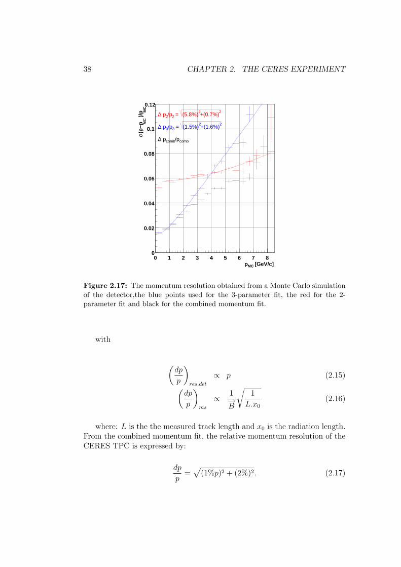
38 CHAPTER 2. THE CERES EXPERIMENT
[GeV/c]MCp0 1 2 3 4 5 6 7 8
MC
)/p
MC
(p−
pσ
0
0.02
0.04
0.06
0.08
0.1
0.122
+(0.7%)2
(5.8%) = 2/p2 p∆
2+(1.6%)
2(1.5%) = 3/p3 p∆
comb/pcomb p∆
Figure 2.17: The momentum resolution obtained from a Monte Carlo simulationof the detector,the blue points used for the 3-parameter fit, the red for the 2-parameter fit and black for the combined momentum fit.
with
(dp
p
)
res.det
∝ p (2.15)
(dp
p
)
ms
∝ 1−→B
√1
L.x0
(2.16)
where: L is the the measured track length and x0 is the radiation length.From the combined momentum fit, the relative momentum resolution of theCERES TPC is expressed by:
dp
p=
√(1%p)2 + (2%)2. (2.17)

2.7. THE CERES TIME PROJECTION CHAMBER 39
2.7.6 Particle identification using dE/dx measurement
Using the TPC, a particle identification of charged particles can be achievedby measuring their energy loss dE/dx. This works very well for particleshaving low momentum, however in the opposite case, when their energyrises, the energy loss of a particle become less mass-dependent and since it isa function of its velocity, it will be hard to separate particles with velocitiesυ > 0.7c. The dE/dx of particles is described as the Bethe-Bloch formulain Eq.(3.6). The energy loss of a particle with charge Z and speed β = υ
c
passing through a medium with the density ρ is given by:
dE/dx = Kq2Z
A
1
β
(1
2
2mec2β2γ2Tmax
I2− β2 − δ
2
)(2.18)
where K = 4πNArec2, NA the Avogadro number, re the electron ra-
dius, Z the atomic number of the absorber, A the atomic weight of theabsorber,γ = 1/
√1− β2, Tmax the maximum kinetic energy in a single col-
lisions, I the mean excitation energy and δ is the Bethe-Bloch correctionfactor.Figure 2.18 shows the energy loss of the observed charged particles in theCERES TPC as a function of the momentum particles and compared withthe Bethe-Bloch formula described above.
log(p [GeV/c])-2 -1 0 1 2 3 4 5
TP
C d
Ed
x [A
.U.]
0
200
400
600
800
1000
1200
1400p
π
K
D
e
Figure 2.18: The energy loss of charged particles as a function of their momen-tum.The lines indicate the predicted dE/dx areas by the Bethe-Bloch formula forπ, K, ρ, d and e

40 CHAPTER 2. THE CERES EXPERIMENT

3The Data Analysis
This chapter described in greater details the neutral pion analysis with em-phasis on the proof and justification for making various cuts. Applying setof selection criteria to track condidates to reject combinatorial background.These choices and the obtained results for the electron/positron selection,the photon reconstruction and then reconstruction of the neutral pion fromthe converted photons in the RICH2 mirror will be discussed in this chapter.
3.0.7 Event data base
The data presented here were taken in the year 2000. The CERES/NA45experiment has recorded on tape a large data samples consisting of 30 milliongood event in Pb-Au collisions of heavy nuclei at beam energy 158 GeV/chaving a centrality of the top 7%(20%) of the total geometric cross sectionwith an average multiplicity of < dNch/dy >= 321 and the pseudorapidityrange η = 2.1 − 2.65. The typical Pb beam intensities delivered to CERESfrom the SPS was ∼ 1 × 10⁶ ions per burst corresponding to a total inter-action rate of 300 ∼ 500 event/burst. The highly compressed raw data ontape coming from the detectors and written by the Data Acquisition System(DAQ) have to be unpacked and converted into a suitable format for thesubsequent data analysis. The events are grouped into 415 units, each unitconsisting of about 200 bursts.The analysis is/was performed in the framework of the C++ software packageCOOL (Ceres Object Oriented Library) with all the functionality needed tohandel and analyze a large amount of data in a very efficient way. Having the
41

42 CHAPTER 3. THE DATA ANALYSIS
data defined as ROOT Tree format specialized storage methods are used toget direct access and process. A complete particle trajectories reconstructedonce all data has been processed into meaningful physical information (i.e.for each particle track a necessary information from each detector is storedlike hit amplitudes and number of hits ..).
3.1 The reconstruction chain
The different steps of the reconstruction chain to get the signal In describingthis, we shall keep the chronological order of the analysis program which canbe represented by the following scheme:
• Hit reconstruction and tracking.
• Electron identification.
• Pairing e+e− −→ γ.
• Identification of γ conversions.
• Pairing γ.
• Invariant mass of π0 in the same event.
• Mixed event and background substraction.
• Invariant mass of π0 as a function of pt and y.
• Efficiency and acceptance determination.
• Efficiency and acceptance correction.
• Transverse momentum spectrum of π0.
The first point is common to all physics analysis done with CERES data.The other steps are specific for the analysis presented here. Therefore, theywill be described in chapter 4 and 5.

3.2. THE ELECTRON AND POSITRON SELECTION 43
3.2 The Electron and Positron selection
The particle identification (PID) in the TPC using the energy loss dEdx ofthe charged particles , provide a powerful tool to select electrons, positronsand to separate them from kaons, pions and protons. As we’ve seen in theprevious chapter, what we called dEdx, a function of mass and momentumof the charged particle which passes through the medium. The momentumis determined by the curvature of the track due to the magnetic field. Thisoperation of particles identification in the TPC is measured from the elec-trons collected at the ends caps of the TPC.The energy loss inside the TPC gas which interest us here is essentially due tothe ionization and to inelastic collisions (gas atoms excitation). The energytransfers which taking place during the Colombien shock have a statisticalcharacter (Landau (ref A) and Vavilov (ref B) distribution). Precise mea-surement of each point (hit) of track which contains a record of 3 chargesadjacent pads is therefore a sample of the energy loss. If the transferred en-ergy to the electron is sufficient, the freed electron thus ionizes other atomsof the gas.
P (GeV/c)0 0.5 1 1.5 2 2.5 3 3.5 4 4.5 5
dE
/dx
(arb
.un
it)
0
100
200
300
400
500
600
dE/dx Charged Particles
P (GeV/c) 0 0.5 1 1.5 2 2.5 3 3.5 4 4.5 5
dE
/dx
(arb
.un
it)
0
100
200
300
400
500
600dE/dx Postirton/Electrons
Figure 3.1: The energy loss of the charged partilces.

44 CHAPTER 3. THE DATA ANALYSIS
Figure (3.1) shows evident points concentration distribution (bands), eachcorresponding to a specific mass of particle. This function that was expressedwithin the equation (2.18) gives a curve as a function of the particle energythat is characterized by a decrease leading to a minimum which is then fol-lowed by a rapid increase that cap. This means that the resolution is good atlow momentum and it became gradually deteriorated when the momentumincreasing. In order to optimize the efficiency and significance, tighter selec-tion criteria are imposed to select only the provided dE/dx information forthe electron and the positrons events. The right of the figure (dEdx figure)represents all the accepted charged particles after taking the dE/dx band inthe region 308 − 2σdEdx < dEdx < 440 and along the momentum interval.However, this cut prevent the contamination of the charged pions when theirsenergy loss overlap. This contamination is clearly visible on the left of thefigure. An extra condition on the momentum is then nedded. The new cutdEdx > 260 + 10logp is included and represented by the the black inclineline which allow the suppression of the π± contaminations and beyond thesevalues.The effect of the previous cuts is showen on the righ side of the figure. Theelectron/positron band are well seperated from the other hadrons, therforethe contaminations can be easily rejected by imposing all the cuts describedabove.
3.3 The mixing event method
Experimentaly we are dealing some times with instabilities particles whichhave a very short life time, or discussing the statistical analysis od datawhich direct to the final event analysis, in these cases we are beyond multiplepaths that lead from the detection digitizings to physics information. Duringthe an ultra-relativistic collosion, a pair of electrons/positrons (i.e the samesigns) do not come from the same photon, however they might issued froma coincidence events.
Figure ( 3.9) shows the reconstructed electron (positron) numbers in eachevent can reach of 32 electron(positron). Each electron (positron) combinewith with positron (electron) of opposit charge to form one photon. Howeverthe extraction of photon signal is reproduced by builiding invariant massdistribution using electrons and positrons hits taken from different event ofsimilar multiplicity.This approach of the substraction of combinatorial background is called themixed event method. The idea of mixed event method is based on the com-

3.3. THE MIXING EVENT METHOD 45
negMultEntries 2.804705e+07
Mean 30.03
RMS 7.725
number of electrons
0 10 20 30 40 50 60 70 80 90
Co
un
ts
0
200
400
600
800
1000
1200
1400
310×
negMultEntries 2.804705e+07
Mean 30.03
RMS 7.725
Electrons posMultEntries 2.804705e+07
Mean 32.47
RMS 8.02
number of positrons
0 10 20 30 40 50 60 70 80 90
Co
un
ts
0
200
400
600
800
1000
1200
1400
310×
posMultEntries 2.804705e+07
Mean 32.47
RMS 8.02
Positrons
Figure 3.2: The multiplicities of electrons and positrons in each event. Theselection was obtained by using the energy loss information. provided from TPCdetector.
bination of the uncorrelated two different electrons or positrons. The super-position of the opposed signs pirs (electrons and positrons) is what define tous the signal and the combinatorial background.
Figure (3.2) shows the principe of the mixed event technique. The ap-plied track selecton is the same for all the recoreded events in order to re-produce correctly the combinatorial background. Each combination for acertain event i between Xi and Yi is taken into acount after passing all theglobal criteria cuts. The yield will form the real distributions needed laterto extract the signal. This step is repeated over all the number of events(n).Another correlation of X and Y particles which can be happened numeri-cally but it will not be taken into acount physicaly since it is considered asbackground. All the combinations Xi and Yi, Yi−1, Yi−2, ...,Yi−n or Yi and Xi,Xi−1, Xi−2, ...,Xi−n are counted by the mixing between the different events.Chronologically, after each event, the selected X−Y combinations are storedin an array.

46 CHAPTER 3. THE DATA ANALYSIS
Xi Yi−2Yi−1 Yi−n
Xi−2Yi
.........
Xi−nXi−1
Yi−4
Event = i
.......Xi−3
Realdistribution
Mixing eventdistribution
Selection of the
lepton pairslepton pairsSelection of the
XiYi
Figure 3.3: The principal operation of the mixing event method.

3.4. THE STANDARD QUALITY CUT 47
3.4 The standard Quality cut
The track quality criteria is used to accept only the well defined tracks andreject the fake tracks. The track quality cuts depends essentially on thenumber of the hits on the track. The main requierment is that the track musthave a minimum number of associated hits. Furthermore, the geometry ofthe TPC detector provide the acceptance range for the whole track findingprocess.
Theta_TPC (rad) 0.1 0.12 0.14 0.16 0.18 0.2 0.22 0.24 0.26 0.28
Hit
s P
er T
PC
Tra
ck
0
2
4
6
8
10
12
14
16
18
20
22
0
1000
2000
3000
4000
5000
6000
7000
8000
9000310×
Figure 3.4: The scatter plot of the used track quality cut. The black line indicatesthe placed criteria dependence on the polar angle and the number of the fitted hits
The recorded number of hits on the TPC segment Only the tracks whichthey have more than 10 hits will be kept for the analysis porformed later. Weapply an angular cut on the polar angle as function of the number of fittedhits to have the full coverage of the TPC detector. This can be summarizedby suspecting the black line indicated in the Figure (3.4). It illustrates theθ of the TPC Vs number of the fitted hits on the stored track. These cuts,on the number of the fitted hits ant the polar angle of the TPC collectivelyreferred to the total TPC geometrical acceptance.

48 CHAPTER 3. THE DATA ANALYSIS
nHits Per TPC Track0 2 4 6 8 10 12 14 16 18 20 22
Co
un
ts
0
200
400
600
800
1000
1200
610×
Figure 3.5: The distribution of the number of the TPC fitted hits
3.5 The study of the unlike and like sign pairs
In our case, as first step from the reconstruction scheme, we start firstly bythe electron/positron combinations and the same procedure will be appliedto γγ invariant mass distributions.Let’s now reformulate the mixed event method explained above to study thephoton reconstruction case. As first point, the X − Y combination whichbasically represents the phase spaces of the associated particles, will be theelectron-positron combination. This latter ensemble of the opposed signs rep-resents the signal of a ”good” photon(from the event).Before going to discuss the photon reconstruction part, we have to keep inmind that we are concerned with the reconstruction of photons that con-vert(shortly) before the TPC spectrometer into e+e− via the measurementof the electron pair in the TPC.The opening angle distribution of the unlike sign pairs (e+e−) and the likesigns pairs (e+e+ + e−e−) for different Pt have been investigated in order tooptimize the definition of the photon for efficiency and significance.The opening angle between the the electron and the positron can be ex-pressed by the equation:

3.5. THE STUDY OF THE UNLIKE AND LIKE SIGN PAIRS 49
cos θ =px1px2 + py1py2 + pz1pz2
|p1||p2| (3.1)
where the P1 and P2 are the Lorentz vector for the electron (positron) andthe positron respectively.The variation of the opening angle between the unlike signs pairs (e+e−) andthe like-sign pairs(e+e+ + e−e−) is shown in figure (3.6).The peak in each momenta window indicates clearly the existance of pho-tons converted before the the Time Projection Chamber. The peak becamenarrower and the number of the photons is descreasing when we go at highmomentum regions.

50 CHAPTER 3. THE DATA ANALYSIS
(rad)θ0 0.005 0.01 0.015 0.02 0.025 0.03 0.035 0.04 0.045 0.05
Co
un
ts
400
600
800
1000
1200
1400
16003
10× theta12unlike0
(rad)12
θ0 0.005 0.01 0.015 0.02 0.025 0.03 0.035 0.04 0.045 0.05
Co
un
ts
1000
1500
2000
2500
3000
3500
4000
4500
5000
310× theta12unlike1
(rad)θ0 0.005 0.01 0.015 0.02 0.025 0.03 0.035 0.04 0.045 0.05
Co
un
ts
500
1000
1500
2000
2500
3000
310× theta12unlike2
(rad)θ0 0.005 0.01 0.015 0.02 0.025 0.03 0.035 0.04 0.045 0.05
Co
un
ts
400
600
800
1000
1200
1400
1600
310× theta12unlike3
(rad)θ0 0.005 0.01 0.015 0.02 0.025 0.03 0.035 0.04 0.045 0.05
Co
un
ts
400
600
800
1000
1200
310× theta12unlike4
(rad)θ0 0.005 0.01 0.015 0.02 0.025 0.03 0.035 0.04 0.045 0.05
Co
un
ts
200
300
400
500
600
700
800
900
1000
310× theta12unlike5
(rad)θ0 0.005 0.01 0.015 0.02 0.025 0.03 0.035 0.04 0.045 0.05
Co
un
ts
100
200
300
400
500
600
700
8003
10× theta12unlike6
(rad)θ0 0.005 0.01 0.015 0.02 0.025 0.03 0.035 0.04 0.045 0.05
Co
un
ts
0
50
100
150
200
250
300
310× theta12unlike9
Figure 3.6: The variation of the opening angle between the unlike sign e+e− (blueline)and the like signs e+e+, e−e− (red line) corresponding to theirs momentumfrom 0 to 8GeV , each window represent 1GeV .

3.5. THE STUDY OF THE UNLIKE AND LIKE SIGN PAIRS 51
At this stage, the conversion signal and the background distribution havedifferent shapes, this can be obsereved by inspecting the unlike and likesingns distributions where the unlike and like signs distributions are notcomparable at each other at low opening angle regions. Further and detailedinvestigations should reveal for a better precision and determination of theopening angle.The ratio of the unlike-signs and like-sign pairs in different momentum bins isdisplayed in the the set of figure (3.7) then it is fitted by a sum of a constantand exponotial functions which take the form:
f(ratio) = p0 + exp(p1 + p2x) (3.2)
The vertical lines in each momentum bin was calculated as the opening anglepoints where the ratio is 10% higher than the constant level (p0). Thislead us to what we call it the cross-point , where the unlike and like signdistributions starts to converge and meet each other. Thereby, bringing thesignal to background ratio to probe the conversion signature gives us theCrosspoint definition expressed by the following equation:
Cross− point(momentum) = 1/p2.(ln(0.1.p1)− p1) (3.3)
where p1 and p2 referes to the fit function parameters metioend previously.Most interestingly, we shall see that the calucaltion of the Cross-point valuesas function of momentum direct us to new physical picture by appling new cuton the opening angle between the the e+e− as function of theirs momentum.From these considerations, we can define the ThetaEP cut. It is shown infigure (3.8)..... and it can be expressed by:
ThetaEP(p) = f1 + f2 (3.4)
where:
f1 = exp(a0 + a1p + a2p2 + a3p
3) with p ∈ [0, 8.5] (3.5)
and
f2 = 3.5 (mrad) (3.6)
f1 function corresponds to the cureved line and f2 is the horizontal lineat the opening angle 3.5(mrad) and larger than 8.5(GeV/c).

52 CHAPTER 3. THE DATA ANALYSIS
(rad)θ0 0.002 0.004 0.006 0.008 0.01 0.012 0.014
Rat
io
0
10
20
30
40
50theta12unlike0
(rad)θ0 0.002 0.004 0.006 0.008 0.01 0.012 0.014
Rat
io
0
10
20
30
40
50
theta12unlike1
(rad)θ0 0.002 0.004 0.006 0.008 0.01 0.012 0.014
Rat
io
0
5
10
15
20
25
30
35
40
45
theta12unlike2
(rad)θ0 0.002 0.004 0.006 0.008 0.01 0.012 0.014
Rat
io
0
5
10
15
20
25
30
theta12unlike3
(rad)θ0 0.002 0.004 0.006 0.008 0.01 0.012 0.014
Rat
io
2
4
6
8
10
12
14
16
18
20
theta12unlike4
(rad)θ0 0.002 0.004 0.006 0.008 0.01 0.012 0.014
Rat
io
2
4
6
8
10
12
theta12unlike5
(rad)θ0 0.002 0.004 0.006 0.008 0.01 0.012 0.014
Rat
io
1
2
3
4
5
6
7
8
theta12unlike6
(rad)θ0 0.002 0.004 0.006 0.008 0.01 0.012 0.014
Rat
io
1
1.2
1.4
1.6
1.8
2
2.2
2.4
2.6
theta12unlike9
Figure 3.7: The ratio of the unlike sign e+e− and the like signs e+e+, e−e− Vsthe opening angle corresponding to their momentum from 0 to 8GeV , each windowrepresent 1GeV . The vertical line indicates the angular cut.

3.6. THE PHOTON RECONSTRUCTION 53
The geometrical ThetaEP cut has its main support at small openingangles and low momenta. In what follows, the ThetaEP cut will kept duringthe whole analysis schem described later.
P (GeV/c)
0 2 4 6 8 10
Op
enin
g a
ng
le (
rad
)
0.003
0.004
0.005
0.006
0.007
0.008
0.009
0.01
0.011Theta(e+e-) Vs P
Figure 3.8: The electron-positron opening angle Vs the momentum, the curevedand the horizontal line indicates the applied cut values to define photons.
3.6 The photon reconstruction
3.6.1 Photon-Matter interaction
Photons are electromagnetic radiations with zero mass, electrically neutraland travelling with a constant velocity that is always the speed of light c. Aphoton passing through material interact in different ways.There are four important mechanisme of interactions between the photonand matter. In all these mechanisms of the process, the photon gives upsome or all of its energy to a matterial particle. This is usually happening inthe vicinity of an atomic nucleus. The Compton effect where the photon can

54 CHAPTER 3. THE DATA ANALYSIS
be diffused by an electron(or a nucleus) and loose some of its energy. Notethat the photon don ot slowdown. It is still travelling with the velocity c,but its frequency is reduced. At lower energies the dominant process is thephotoelectric effect.The photon collide with the electron and ionizes the atom of the matterialby kicking out one electron.Other process equivalent to the previous one but in this case the photonenergy is not enough to free the electron. Thereby, the photon is capturedby the atom and excites the state of the hitted electron in the shell to higherenergy level. Again, the photon disappears and transmits all its energy tothe atom. The Last common process, which is the formation or the materi-alization of two electrons, one negative (electron) and the other one positive(positron). This process is called Pair production. It is a direct conversionof radiant energy to matter
3.6.2 Photon conversions (γZ −→ e+e−Z)
The CERES/NA45 experiement measures photon yields by conversion method.For Pair Production to occur, the electromagnetic energy ,or the photon en-ergy, must be at least equivalent to the mass of the two electrons. Whenthe photon energy is greater than 2mec
2, which corresponds to 1.022MeV ,the photon can be materialized bu the creation of electron-positron pair. Forphoton energies above the threshold energy, the surplus energy appears askinetic energy to the two electrons.An additional condition which must be satisfied during the Pair Productionprocess because it can not be occur in the vacuum. The energy and the mo-mentum can not be simultaniusly conserved. Something must participate inthe interaction and absorb the momentum of the inital photon to balance theequations. The presence of a charged particle line an atomic nucleus, whichshould be more massive than the electron/positron, during the interactioncan absorbe a fraction of the photon mometum. The Pair Production is thedominant process at high energies.Since the photons are masseles, they are not detected directly. Theirs stateis displaced as neutral vertex. The converted electrons are identified by thesearching for oppositely charged track near the eletron track, then we dothe extrapolatation to a common target point. Tracks found in this way aresubsequently used as starting point for track combinations and a convertedphoton is created for each valid pair. We have to remember that our our goalis to reconstruct the photons through conversions happening mainly in theRICH2 mirror location.

3.6. THE PHOTON RECONSTRUCTION 55
3.6.3 The reconstructed photon mapping
So far we have concentrated on the description of the unlike and like signpairs as building blocks for the photon by using the TPC information. Thenumber of photons per each event is displayed in figure (??). Our next taskis to define and determine the photon by scanning theirs spatial map insidethe detector.
Gamma_unlikeS
Entries 2.804705e+07
Mean 2.836
RMS 1.801
number of photons0 2 4 6 8 10 12 14
Co
un
ts
0
5
10
15
20
25
30
35
40
45
610×Gamma_unlikeS
Entries 2.804705e+07
Mean 2.836
RMS 1.801
Photons
Figure 3.9: The number of the reconstructed electrons and positrons in eachevent by using the dEdx information provided from TPC detector.
Figure ( 3.11) illustrates the azimuthal and the polar angles distributionsfor the primary photon selection based on the data collected previousely. Inthe X-Y plane, the photons are measured for the whole azimuthal acccep-tance. However. a radiant cut 0.135 ≤ θ ≤ 0.25 was used to select onlythe phase-space where the photons are supposed to come from the decay ofthe neutral pions. Thus, by appling this polar cut we exclude the photonsyielded from the multiple scattering or the Bremmstralung processes whichare mainly happening at lower polar angles. The measured transeverse mo-mentum of the reconstructed primary photon from the the unlike and likesign pairs is shown in Figure (3.10). The transverse momentum distributionhas sharp peak near zero and broader peak at high transeverse momentum.This behaviour can be understood from the fact that photon conversion iscaraterised by very small electron-positron opening angle.
The measured transeverse momentum vector for the primary photonFor the preceding considerations, the plan for the start-up should therefor
be two-pronged. The first one is the sophisticated reconstruction of the sec-

56 CHAPTER 3. THE DATA ANALYSIS
(GeV/c)tP1 2 3 4 5 6
Co
un
ts
1
10
210
310
410
510
610
(GeV/c)tP0.2 0.4 0.6 0.8 1 1.2 1.4 1.6 1.8
Nu
mb
er o
f P
ho
ton
s
0
200
400
600
800
1000
1200
1400
310×
Figure 3.10: Schematic event display of the TPC.
ondary verticies, and later on a very good approach will be applied by makinga cut on the converted photon at the RICH2 mirror position. The recon-struction scheme and further explanations of the Secondary Vertex Techniquewill be described later.
3.7 The Secondary vertex fit algorithme
The Secondary vertex technique provide a very clean and well measured pho-tons which can be used in the reconstructed of the neutral pions representedin the next section. Opposite charged trackes are combined to obey thephysical process γ −→ e+e− condidates. The method will be expanded toprovided the option to fit the charged tracks. Each of the two tracks is as-sumed to point out to a common position. This constraint take into acountthat the verticies are parallel to each other at the conversion point as a gen-eral assumption. Consequently, an implicit ”zero mass” on the invariantmass for the displaced vertices is yielded at the RICH2M region.The principle of the Scondary Vertex fit algorithme is to calculate the 3Ddistance between the two tracks. The used alogorithme calculates the pointof the opposit sign track pairs which have assigned to the electron and tothe positron. This method is performed on the Least Square Method. It wasused by HADES colloboration, and it is also described in [HADES reference].For further details and all the characteristic features about it the reader isadvised to consult [reference].The study of the vertexing and kinematic fitting withing the Secondary Ver-

3.7. THE SECONDARY VERTEX FIT ALGORITHME 57
(rad)φ-3 -2 -1 0 1 2 3
(ra
d)
θ
0.1
0.12
0.14
0.16
0.18
0.2
0.22
0.24
0.26
0.28
0.3 Gamma mapping
(rad)θ0.1 0.12 0.14 0.16 0.18 0.2 0.22 0.24 0.26 0.28 0.3
Co
un
ts
0
200
400
600
800
1000
1200
1400
1600
310× Gamma: Theta
(rad)φ-3 -2 -1 0 1 2 3
Co
un
ts
0
100
200
300
400
500
600
700
800
900
310× Gamma: Phi
Figure 3.11: The mapping of the reconstructed photons in the phase-space. Thetop window represents the bidimentional distribution of the azimuthal and polarangles for the reconstructed photons. The middel and the bottom windows showsthe projection of the thetaγ and the φ angles respectively.
tex algorotihme will be devided into two subsections. The first part will be

58 CHAPTER 3. THE DATA ANALYSIS
intended to provide the mathematical framework of the vertex fitting. This ishandled generaly by solving analytically the closest approch point equationsof the two opposit sign tracks. Then we will examine in more details and ex-plicitly the practice ccalculation of the cloeset approach point occuring fromthe latter subsection.
3.7.1 The mathematics of the Secondary Vertex fit
The general way of the Secondary Vertex consitits of the following perscrip-tion. All the charded tracks are parametrized as straight lines and used asinput to the algorithme. Assuming that there are N detected tracks thatmeans for each input condidate i ∈ [1, N ] and from the linearity hypothesis,we write the definiton of the ith track in the form:
~xi = ~ri + ~ui.t, t ∈ < (3.7)
such that ~ri refers to the position vector, ~ui its direction vector,i.e. ~ui =~ri/|~ri| and t is the track parameter or the so-called controlled varialble. Wewill attempt to determine the unkown coordinates is space of the positionvector ~rsv which is assigned to the point of conversion. The distance ofthe conversion point to a given ith track which is basically expressed in theequation (3.7) can be calculated as:
Di = |(~ri − ~rsv)× ~ui| (3.8)
Equation 2 is a reslut from the the fact that ~ri vector set are the measureddata points and the Di represents the deviations from the the given set ofdata in the base |~ui|. According to Least Square method, the fitting proceedsby finding the sum of the squares of the deviations Di for all the detectedtracks. There are a given uncertantities for all the measured data point;for that reason these points can be weighted differently in order to give thehigh-quality points more weight. Based on this, the squares deviations aretherefore summed and minimized to find the best fit line. This can yieldsthe following:
M2 =N∑
i=1
D2i
σ2i
=N∑
i=1
|(~ri − ~rsv)⊗ ~ui| (3.9)
By taking the uncertanties σ2i constant, the minimization ofM2 is thus equiv-
alent to the determination of the space coordinates of the closest approachbetween the N tracks. The minimization of M2 is simply done by makingthe the partial derivatives of M2 with respect to the unkown parameters andset these value to zero. The M quantity defined in Eqution 3 has a properity

3.7. THE SECONDARY VERTEX FIT ALGORITHME 59
which can be used to carry out a χ2 test. We now write this consequence,the analogous expression of 3, in the form:
χ2 =N∑
i=1
D2i
σ2i
(3.10)
The condition for the χ2 to be minimum is that:
∂χ2
∂xsv
= 0,∂χ2
∂ysv
= 0,∂χ2
∂zsv
= 0 (3.11)
To determine the equation(3.11), we first have to get the distance betweenthe two selected charged traks D2
i .i.e.:
D2i = [(yi − ysv)azi − (zi − zsv)ayi]
2
+[(zi − zsv)axi − (xi − xsv)azi]2
+[(xi − xsv)ayi − (yi − ysv)axi]2 (3.12)
Expanding the equation system (3.11), this leads to:
∂χ2
∂xsv=
∑Wi {[(zi − zsv)axi − (xi − xsv)azi]azi − [(xi − xsv)ayi − (yi − ysv)axi]ayi} = 0
∂χ2
∂ysv=
∑Wi {[(xi − xsv)ayi − (yi − ysv)axi]axi − [(yi − ysv)azi − (zi − zsv)ayi]azi} = 0
∂χ2
∂zsv=
∑Wi {[(yi − ysv)azi − (zi − zsv)ayi]ayi − [(zi − zsv)axi − (xi − xsv)azi]axi} = 0
(3.13)
where theWi is the wieghting factor 2/σ2i The equation (3.13) is linearized
in the unkown parameteres of the space coordiantes. Involving matrix manip-ulations and especialy matrix inversions, the equation system in (3.13) canbe summarized in three main matricies labeled as A, B and C which satisfythe equation:
C = A−1B (3.14)
The expressions of these specific matricies are written in the matrial formand obtained as follow:
A =N∑
i=1
Wi
a2yi + a2
zi −axiayi −axiazi
−ayiaxi a2xi + a2
zi −ayiazi
−aziaxi −aziayi a2yi + a2
xi
(3.15)

60 CHAPTER 3. THE DATA ANALYSIS
B = A
xi
yi
zi
, (3.16)
and the wanted matrix:
C =
xsv
ysv
zsv
, (3.17)
One this problem is handled by solving analytically the point of closest ap-proach of the two charged tracks (the two candidates), we could then deter-mine the A,B and C matricies. The latter C matrix is 1−column matrixwhich offers the space coordinates values of the conversion point..It may be, however, that the uncertanties σi are not normally distributed.and theirs expectation values are different from zero. This constraint impliesdependency of the σi uncertantities on the Di distances(i.e. σ2
i = σ2i (Di)).
In this case special care on the calculation of σi‘s values because we are deal-ing with non-negligible values of errors. It can be redefine and one gets thealternative expression as:
σ2i (Di) =
(∂Di
∂x1
,∂Di
∂y1
,∂Di
∂x2
,∂Di
∂y2
)
σx1x1 0 σx1x2 00 σy1y1 0 σy1y2
σx2x1 0 σx2x2 00 σy2y1 0 σy2y2
∂Di
∂x1∂Di
∂y1∂Di
∂x1∂Di
∂y2
(3.18)
With the definition written in equation (3.18), (x1, y1) refers to the trackspace coordinates by requiring z = 0. (x2, y2) are the corresonding slopes inthe X-Z plane (for x2) and Y-Z palne (for y2). Thus, that reads:
x2 =ux
uz
y2 =uy
uz
(3.19)
where (ux, uy, uz) are the coordinates of the unit direction vector ~u. The σmn
refers to covariance if m 6= n and in the opposit case m = n it correspondsto the variance of the m and n parameters. In what follows, we will use ashort notations to simplify the complication of the equations. Let:

3.7. THE SECONDARY VERTEX FIT ALGORITHME 61
~∆i = ∆x~i+ ∆y
~j + ∆z~k. (3.20)
and
~∆i = ~ri − ~rsv. (3.21)
from the equations (3.20) and (3.21) one can gets:
∆x = xi − xsv
∆y = yi − ysv
∆z = zi − zsv
(3.22)
Furthermore, the unit vector properity provide us:
u2z = 1− u2
x − u2y (3.23)
which leads to:
∂uz
∂ux
= −ux
uz
,
∂uz
∂uy
= −uy
uz
(3.24)
From these formulas, the equation 3.12 can be re-written in the followingcompact form:
D2i = (∆2
zi −∆2xi)u
2xi + (∆2
zi −∆2yi)u
2yi − 2(∆yi∆ziuyiuzi)
+∆xi∆ziuxiuzi + ∆xi∆yiuxiuyi.+ ∆2xi + ∆2
yi (3.25)
and the partial derivatives in equation 3.18 will be computed with respectto ux and uy and not for the x2 and y2 cases (this step will be done later).Thus, the results of the updated partial derivatives of the distance Di areand obtained as:

62 CHAPTER 3. THE DATA ANALYSIS
∂Di
∂x1
=(1− u2
xi)∆xi − uxi(∆ziuzi + ∆yiuyi)
Di
∂Di
∂y1
=(1− u2
yi)∆yi − uyi(∆ziuzi + ∆xiuxi)
Di
∂Di
∂uxi
=(∆2
zi −∆2xi)uxi +
∆yi∆ziuyiuxi
uzi+
∆xi∆ziu2xi
uzi−∆xi∆ziuzi −∆xi∆yiuyi
Di
∂Di
∂uyi
=(∆2
zi −∆2yi)uyi −∆yi∆ziuzi + ∆yi∆zi
u2yi
uzi+ ∆xi∆zi
uxiuyi
uzi−∆xi∆yiuxi
ui
.
(3.26)
The remaining partial derivatives values of (∂Di/∂x2) and (∂Di/∂y2) arethen straightforward obtained from the previous step. This yields:
∂Di
∂x2
=∂Di
∂uxi
.∂uxi
∂x2
+∂Di
∂uyi
∂uyi
∂x2
=∂Di
∂uxi
.1− u2
xi
Q− ∂Di
∂uyi
.x2y2
Q3(3.27)
∂Di
∂y2
=∂Di
∂uxi
.∂uxi
∂y2
+∂Di
∂uyi
.∂Dyi
∂y2
= − ∂Di
∂uxi
.x2y2
Q3+∂Di
∂uyi
.1− u2
yi
Q, (3.28)
with
Q = x22 + y2
2 + 1 (3.29)
Using the equations in 3.19, Q can be expressed in the form:
Q =1
u2z
(3.30)
Finally, once all the parametters have been found, the error propagationwith the no-negligible values of σi is obtained by simply implimenting all ofthem in the euqation ( 3.18).The complete procedure is re-iterated until convergence is reached. Beforeeach iteration track parameteres and error matricies are translated to cur-rent vector position. It should be noted that the procedure of the chargedtrack selection for the conversion criteria is iterated till a displacement of theorder 0.01µm or less is seen on the computed slope of the secondary vertexposition.As a conlusion, the method is based on mximazing the Secondary vertexprobability (or minimizing the χ2) derived from the vertx fits for a permuta-tion of possible two track associations. Within the mathematical framework,the position of the conversion point is then given by the equation ( 3.14).

3.7. THE SECONDARY VERTEX FIT ALGORITHME 63
3.7.2 Application of the Secondary vertex method
The determination of the Secondary vertex point manifest through the math-ematical configuration presented above. As a consequence, here we make adirect application for the photon conversion point which is identified by thefollowing sequence.
~a2
~p2
~p1
z
y
t~b1
x
~a1
s~b2
~d
Figure 3.12: Fey.Diag
...... le dessin .............
Assume we have the two electrons vectors expressed as:
{~p1 = ~a1 + t.~b1
~p2 = ~a2 + s.~b2(3.31)
we consider the distance vector ~di between ~p1 and ~p2, that means:
~di = u(~b1 ×~b2) ⇔ ~di⊥~b1 and ~di⊥~b2 (3.32)
In additon one can get (see Figure ..):
~p1 + ~di = ~p2 (3.33)
~a1 + t.~b1 + u(~b1 ×~b2) = ~a2 + t.~b2 (3.34)
which yields:
~a1 − ~a2 = s~b2 − t~b1 + u(~b1 ×~b2) (3.35)

64 CHAPTER 3. THE DATA ANALYSIS
By re-writting the equation ( 3.35) in the matricial form:
b2x −b1x (~b2 ×~b1)x
b2y −b1y (~b2 ×~b1)y
b2x −b1z (~b2 ×~b1)z
stu
=
a1x − a2x
a1y − a2y
a1z − a2z
(3.36)
The goal is to determine (s, t, u) vector compount. The system of linear equa-tions in ( 3.36) can be soveld by using Cramer’s rule in terms of determinants.That read,
s =detS
detA, t =
detT
detA, u =
detU
detA(3.37)
with:
detA =
∣∣∣∣∣∣∣
b2x −b1x (~b2 ×~b1)x
b2y −b1y (~b2 ×~b1)y
b2x −b1z (~b2 ×~b1)z
∣∣∣∣∣∣∣(3.38)
detS =
∣∣∣∣∣∣∣
a1x − a2x −b1x (~b2 ×~b1)x
a1y − a2y −b1y (~b2 ×~b1)y
a1z − a2z −b1z (~b2 ×~b1)z
∣∣∣∣∣∣∣(3.39)
detT =
∣∣∣∣∣∣∣
b2x a1x − a2x (~b2 ×~b1)x
b2y a1y − a2y (~b2 ×~b1)y
b2z a1z − a2z (~b2 ×~b1)z
∣∣∣∣∣∣∣(3.40)
detU =
∣∣∣∣∣∣
b2x −b1x a1x − a2x
b2y −b1y a1y − a2y
b2z −b1z a1z − a2z
∣∣∣∣∣∣(3.41)
Consequently, the Secondary vertex point is just pointed out by the vector~p12 expressed by the following equation:
~p12 = ~p1 +1
2~di (3.42)
= ~p1 +1
2(~p1 − ~p2). (3.43)
Any vector of the electron/postiron detected by the TPC and expressedby the equation (3.33) is then computed by the coordinates (Xline0,Y line0, 0).The (x2, y2) slopes that are defined in the previous section with z = 0 areeuquivalent to the ~s slope in the X-Z plane (for x2) and Y-Z palne (for y2).They are obtained by the Xline1 and Y line1 values of the TPC track. Thelatter two parameteres are used to measure the local angles defined in theequations ( 2.12) and ( 2.13).

3.7. THE SECONDARY VERTEX FIT ALGORITHME 65
3.7.3 Secondary vertex cut (SV)
Since our concern is to reconstruct the photons that converts in the RICH2mirror position, we select them by making a cut on the converted photon. Itwas possible to enhance the extracted photon signal by the ThetaEP cut de-scribed in Section (3.5). It has a powerful support to reduce the backgroundand to compensate the resolution and the sginificance.
Sec.Ver. X (cm)
-150 -100 -50 0 50 100 150
Co
un
ts
610
710
810
910
1010
Sec.Ver. X (cm)-150 -100 -50 0 50 100 150
Co
un
ts
0
500
1000
1500
2000
2500
310×
Sec.Ver. Y (cm)-150 -100 -50 0 50 100 150
Co
un
ts
0
500
1000
1500
2000
2500
3000310×
Sec.Ver. Y (cm)
-150 -100 -50 0 50 100 150
Co
un
ts
610
710
810
910
1010
Figure 3.13: The Secondary Vertex distributions of the photons condidates. Thereconstructed photons from the unlike sign pairs (e−e+) are in bleu and the likesign pairs.(e−e− + (e−e+)) in red. The top two plots correspond to SecondaryVertex distributions on the X axis before and after the ThetaEP cut while onthe bottom two plots, the same distributions on the Y axis before and after theThetaEP cut

66 CHAPTER 3. THE DATA ANALYSIS
This can be seen by checking the reconstrcuted seconday verticies distri-butions in the X,Y and Z axis. It is explicitly verified on the X and Y axisshown in figure (XY) after and before the ThetaEP cut. Addionally, a moreserver check can be observed corresponding the projection of the distribu-tion on the X-Y plane illustrated in figure(3.14). The highly concentrateddistribution represents the photons location in the phase-space.
This method reinforce the suppression of the contamination of differenthadrons and distinguish between them
SV X (cm)-150 -100 -50 0 50 100 150
SV
Y(c
m)
-150
-100
-50
0
50
100
150
0
10000
20000
30000
40000
50000
60000
Figure 3.14: The projection of the Secondary Vertex distribution on the X-Yplane.The most populated area indicates the positions of the reconstructed pho-tons.
A similar situation along the Z axis is presented spearately, where themost significantly photons distribution are very clear. This is shown in figure3.15. From this one finds that reconstructed photons are concenrated in theRICH2 mirror region. This is expected since the RICH2 mirror is mainconverter and leads to acceptable situation.
By following the previous steps discussed above, More precise tunning isnow needed and may give further improvemement to select the photons atthe RICH2M position. The Secondary Vertex cut (SV) can be comfortablyperformed at 2σ. After extensive verification that no photons informationwas being originated from other locations, by keeping the SV cut in all theaccumulated analysis, the Secondary Vertex distributions from the contribu-

3.7. THE SECONDARY VERTEX FIT ALGORITHME 67
Sec.Vertex Z (cm)
0 100 200 300 400 500 600 700 800
Co
un
ts
610
710
810
910
Sec.Vertex Z (cm)
0 100 200 300 400 500 600 700 800
Co
un
ts
0
1000
2000
3000
4000
5000
6000
310×
Figure 3.15: The Z direction of the Secondary Vertex distributions of the photoncondidates before (left) and after (right) imposing the ThetaEP cut.
tions of the unlike and like sign pairs investigated as function of the photonmomentum (see figure (3.18)). This rquierement is a major benefit from theSV cut which has been studied depending on the momentum of the photons.This study can be explored in figure (3.17). The location of the extractedphoton signal is substantially present at the RICH2 converter and fitted withGaussian function. This comfirms that the used technique to determine thephotons is equivalent to our expectations where they should be occuring.
The mean of the Gaussian fit refers to converted photons as functionof theirs momenum. The stability of the mean values indicates the wellreconstructed photons condiates which will be used next to the neutral pionreconstruction. The width of the distributions is dominated by te angularresolution of the opposed chared tracks.

68 CHAPTER 3. THE DATA ANALYSIS
Vertex Z (cm)0 100 200 300 400 500 600 700 800
Co
un
ts
0
200
400
600
800
1000
310×
Vertex Z (cm)0 100 200 300 400 500 600 700 800
Co
un
ts
0
200
400
600
800
1000
1200
1400
1600
1800
2000
2200
310×
Vertex Z (cm)0 100 200 300 400 500 600 700 800
Co
un
ts
0
200
400
600
800
1000
310×
Vertex Z (cm)0 100 200 300 400 500 600 700 800
Co
un
ts
0
50
100
150
200
250
300
350
400
450
310×
Vertex Z (cm)0 100 200 300 400 500 600 700 800
Co
un
ts
0
20
40
60
80
100
120
140
160
180
200
220
310×
Vertex Z (cm)0 100 200 300 400 500 600 700 800
Co
un
ts
0
20
40
60
80
100
310×
Vertex Z (cm)0 100 200 300 400 500 600 700 800
Co
un
ts
0
10000
20000
30000
40000
50000
Vertex Z (cm)0 100 200 300 400 500 600 700 800
Co
un
ts
0
5000
10000
15000
20000
25000
Vertex Z (cm)0 100 200 300 400 500 600 700 800
Co
un
ts
0
2000
4000
6000
8000
10000
12000
14000
Vertex Z (cm)
Figure 3.16: The measured Z direction of the Secondary Vertex distributionsafter the ThetaEP cut as function of the photon momentum.

3.7. THE SECONDARY VERTEX FIT ALGORITHME 69
Z (cm)100 150 200 250 300 350 400 450 500
SV
Sig
nal
0
200
400
600
800
1000
1200
310×
Z (cm)100 150 200 250 300 350 400 450 500
SV
Sig
nal
0
500
1000
1500
2000
2500
310×
Z (cm)100 150 200 250 300 350 400 450 500
SV
Sig
nal
0
200
400
600
800
1000
12003
10×
Z (cm)100 150 200 250 300 350 400 450 500
SV
Sig
nal
0
100
200
300
400
500
310×
Z (cm)100 150 200 250 300 350 400 450 500
SV
Sig
nal
020406080
100120140160180200220
310×
Z (cm)100 150 200 250 300 350 400 450 500
SV
Sig
nal
0
20
40
60
80
100
310×
Z (cm)100 150 200 250 300 350 400 450 500
SV
Sig
nal
02000400060008000
100001200014000160001800020000
Z (cm)100 150 200 250 300 350 400 450 500
SV
Sig
nal
0100020003000400050006000700080009000
Z (cm)100 150 200 250 300 350 400 450 500
SV
Sig
nal
0
500
1000
1500
2000
2500
3000
3500
4000
Z (cm)100 150 200 250 300 350 400 450 500
SV
Sig
nal
0
50001000015000200002500030000350004000045000
Figure 3.17: The extracted signal distribution of the converted photons Vs themomentum of the photon.

70 CHAPTER 3. THE DATA ANALYSIS
P (GeV/c)0 1 2 3 4 5 6 7 8 9 10
Sec
.Ver
. Wid
th (
cm)
10
20
30
40
50
60
70
80
90
100
P (GeV/c)0 1 2 3 4 5 6 7 8 9 10
Sec
.Ver
. Mea
n (
cm)
200
220
240
260
280
300
320
340
360
380
400
Figure 3.18: The mean and the width of the fitted Seondary vertex distributionVs the phton momentum.
3.8 The π0 reconstrcution
This section is dedicated to describe the reconstruction of π0 from γγ decay.The produced π0 decays into a pair of photons with branching ratio 98.7%making it the most convenient decay channel for π0 reconstruction. The pro-cedure to determine the reconstruction is similar to the one for the photonsdescribed in Section (3.6).
3.8.1 Invariant mass analysis
The invariant mass of a particle is given by the absolute value of its 4-momentum. As photons are massless particles this reduces to the determi-nation of the energy and the opening angle between the two photons. Forphoton pair originating from π0 decay the invariant mass is identical to theπ0 rest mass of 134.9766 MeV [19]. The reconstruction of π0 is twofoldproblem. The first one was the reconstruction of the γ. Then π0’s are found.γ’s were reconstructed by combining the two opposed charged traks of e+
and e− unsing the TPC information. The invariant mass of particle pair isgiven by the absolute value of its 4-momentum.
p12 = p1 + p2 (3.44)
The invariant mass expression of π0 −→ γγ is found by taking the

3.8. THE π0 RECONSTRCUTION 71
p = (p0, p1, p2, p3) = (E, pxpypz) and taking the metric base diag gµν =(1,−1,−1,−1). The E = p for the photons. This reads:
M2π0 = 2Eγ1Eγ2(1− cos θ)
= 2|−→pγ1||−→pγ2|(1− cos θ)
=⇒Mπ0 =√
2|−→pγ1||−→pγ2|(1− cos θ) (3.45)
The Mixing event
Once the ”good” photons are identified, the invariant mass analysis of π0
cannot be identified uniquely since all possible photon-photon combinationshave to be considered. The procedure of event mixing method is widely usedto determine the combinatorial background. The mixed event is determinedby taking all photon candidates from an event and combine it with the pho-tons from different events. This straight forward to what have been discussedin Section (3.3). By this way the mixed event distribution is determined inthe case of the π0 invariant mass
The Armenteros Podolanski plots
In order to try to verify if there is any cross decay channels with the π0 peakwhich can be missidentify the mass, we study the Armenteors-Podolanskiplot [20].
|α|0 0.2 0.4 0.6 0.8 1 1.2
(GeV
)tq
0
0.05
0.1
0.15
0.2
0.25
-500
0
500
1000
1500
2000
2500
3000
Arm. Plot
Figure 3.19: The mean and the width of the fitted Seondary vertex distributionVs the phton momentum.

72 CHAPTER 3. THE DATA ANALYSIS
The variables of the Armenteors-Podolanski techinque are the pTA whichis the projection of one of the two photon momentum (daugthers) on theflight direction of the neutral pion (parent). The second used parameter is αthat can define by the momentum projections of the photons on the directionof the π0 meson. This can be simply expressed as:
α =pL(γ1)− pL(γ2)
pL(γ1) + pL(γ2)(3.46)
In the (pTA, α) plane, a good reconstruction of the parent particle massshould appears as an elliptic concentration. This can be seen in figure3.19. This method reinforce the suppression of the contamination of dif-ferent hadrons and distinguish between them. A clear signal of the neutralpion mass is seen and ther is no decay channel which can misidentified thereconstruction of the γγ invariant mass.
The Opening angle cut (OpG1G2)
The opening angle between the two photons have been studied as function ofthe neutral pion transverse momentum. This is shown in figure (3.20). Anopening cut OpG1G2 between the two reconstrcuted photons is implementedin order to reduce the combinatorial background whi are coming from smallopening angle photons. The magenta line indicates the implemented cut asfunction of the neutral pion momenta,this can be expressed as: OpG1G2= 0.2 exp(−5p) + 0.02. where p represents the momenta of the neutral pion.
The π0 signal extraction
The combinatoric background is define as the background level in mass dis-tributions after imposing all the requierements on the kinematic quantities.Besides the discussed cuts, more stringent requirements are used to observethe π0 signal. The combinatorial background depends upon the pT distrib-tuion of the reconstructed photons.The obtained γγ invariant mass distributions for the photons yielded fromthe same event and the mixing event is scanned as function of transversemomentum and rapidity ranges. This has been checked for 10 pt bins. Eachsignal templates represents 0.25(GeV/c). We expand also the study as func-tion of rapidity splited in three interval, 2.2 ≤ y1 < 2.4, 2.4 ≤ y2 < 2.6 and2.6 ≤ y3 < 2.7. In all what follows we will measure the γγ invariant mass asfunction of these two varialbes (pt,y). Additional constraint on the secondpt bin 0.25-0.5 (GeV/c), the third pt bin 0.5− 0.75(GeV/c) and along all therapidity intervals. This cut have been imposed where we require for all the

3.8. THE π0 RECONSTRCUTION 73
(GeV/c)t
: p0π0 0.2 0.4 0.6 0.8 1 1.2 1.4 1.6 1.8 2
op
enin
g a
ng
le (
rad
)
0
0.05
0.1
0.15
0.2
0.25
0.3
0.35
0.4
0.45
0.5
0
10000
20000
30000
40000
50000
60000
70000
80000
90000
Figure 3.20: The scatter plot of the π0 transeverse momenta vs the openingangle between the two photons. The OpG1G2 cut is indicated by the magintaline.
photons opening angles to be larger than 0.11 rad and 0.07 rad in the trans-verse momentum interval 0.25− 0.5GeV/c and 0.25− 0.5Gev/c respectively,and for all the rapidity 2.2 < y < 2.7.All photons that survived the previous cuts were taken in combination witheach other. The resulting γγ mass distributions was used to define the π0
signals. As it is illustrated in figures (3.21), (3.22), (3.23) the signal is wellseperated from the background and the π0 mass is pointed out by the verticalline. The background in bleu is below the peak in all the transeverse mo-menta bins and rapidity. In the first pt window we do not measure photons,therefore no signal is obtained.The scale factor obtained from the ratio (real/mixed) of the invariant massdistribution will be used to normalize the mixed event background and sub-tract it from the real event invariant mass distributions. The normalizationis done with the purpose to have equal width of the mixed to the real condi-dates.The normalization region for each pt and rapidity is obtained by fitting theratio of the γγ mass distribution of the real to the mixed events. The usedfit function for this purpose is gaussian function and a constant.The constantfactor was obtained from the ratio of the two distributions. The range of thefit is 0.08− 0.25(GeV ). (see figures (3.24), (3.25), (3.26) )

74 CHAPTER 3. THE DATA ANALYSIS
(GeV)γ γMass 0 0.05 0.1 0.15 0.2 0.25
Co
un
ts
0
5000
10000
15000
20000
25000
30000
(GeV)γ γMass 0 0.05 0.1 0.15 0.2 0.25
Co
un
ts
0
10000
20000
30000
40000
50000
60000
70000
80000
(GeV)γ γMass 0 0.05 0.1 0.15 0.2 0.25
Co
un
ts
0
10000
20000
30000
40000
50000
60000
70000
80000
(GeV)γ γMass 0 0.05 0.1 0.15 0.2 0.25
Co
un
ts
0
5000
10000
15000
20000
25000
30000
35000
(GeV)γ γMass 0 0.05 0.1 0.15 0.2 0.25
Co
un
ts
0
2000
4000
6000
8000
10000
12000
(GeV)γ γMass 0 0.05 0.1 0.15 0.2 0.25
Co
un
ts
0
500
1000
1500
2000
2500
3000
3500
4000
4500
(GeV)γ γMass 0 0.05 0.1 0.15 0.2 0.25
Co
un
ts
0
200
400
600
800
1000
1200
1400
1600
(GeV)γ γMass 0 0.05 0.1 0.15 0.2 0.25
Co
un
ts
0
100
200
300
400
500
600
Figure 3.21: The invariant mass distribution for all the photons coming from thesame event(blue histogram) and the mixing event (red histogram) for the rapidityrange 2.2 ≤ y < 2.4 and 8 pt bins of 0.25GeV

3.8. THE π0 RECONSTRCUTION 75
(GeV)γ γMass 0 0.05 0.1 0.15 0.2 0.25
Co
un
ts
0
10000
20000
30000
40000
50000
60000
(GeV)γ γMass 0 0.05 0.1 0.15 0.2 0.25
Co
un
ts
0
20
40
60
80
100
310×
(GeV)γ γMass 0 0.05 0.1 0.15 0.2 0.25
Co
un
ts
0
10000
20000
30000
40000
50000
60000
70000
80000
(GeV)γ γMass 0 0.05 0.1 0.15 0.2 0.25
Co
un
ts
0
5000
10000
15000
20000
25000
30000
35000
40000
(GeV)γ γMass 0 0.05 0.1 0.15 0.2 0.25
Co
un
ts
0
2000
4000
6000
8000
10000
12000
14000
(GeV)γ γMass 0 0.05 0.1 0.15 0.2 0.25
Co
un
ts
0
1000
2000
3000
4000
5000
(GeV)γ γMass 0 0.05 0.1 0.15 0.2 0.25
Co
un
ts
0
200
400
600
800
1000
1200
1400
1600
(GeV)γ γMass 0 0.05 0.1 0.15 0.2 0.25
Co
un
ts
0
100
200
300
400
500
600
Figure 3.22: The invariant mass distribution for all the photons coming from thesame event(blue histogram) and the mixing event (red histogram) for the rapidityrange 2.4 ≤ y < 2.6 and 8 pt bins of 0.25GeV

76 CHAPTER 3. THE DATA ANALYSIS
(GeV)γ γMass 0 0.05 0.1 0.15 0.2 0.25
Co
un
ts
0
2000
4000
6000
8000
10000
12000
14000
16000
(GeV)γ γMass 0 0.05 0.1 0.15 0.2 0.25
Co
un
ts
0
2000
4000
6000
8000
10000
12000
14000
16000
18000
20000
(GeV)γ γMass 0 0.05 0.1 0.15 0.2 0.25
Co
un
ts
0
2000
4000
6000
8000
10000
12000
(GeV)γ γMass 0 0.05 0.1 0.15 0.2 0.25
Co
un
ts
0
1000
2000
3000
4000
5000
6000
(GeV)γ γMass 0 0.05 0.1 0.15 0.2 0.25
Co
un
ts
0
500
1000
1500
2000
2500
(GeV)γ γMass 0 0.05 0.1 0.15 0.2 0.25
Co
un
ts
0
200
400
600
800
1000
(GeV)γ γMass 0 0.05 0.1 0.15 0.2 0.25
Co
un
ts
0
50
100
150
200
250
300
350
(GeV)γ γMass 0 0.05 0.1 0.15 0.2 0.25
Co
un
ts
0
20
40
60
80
100
120
140
160
Figure 3.23: The invariant mass distribution for all the photons coming from thesame event(blue histogram) and the mixing event (red histogram) for the rapidityrange 2.4 ≤ y < 2.7 and 8 pt bins of 0.25GeV

3.8. THE π0 RECONSTRCUTION 77
/ ndf 2χ 40.37 / 47p0 0.00011± 0.07351 p1 0.0010± 0.1131 p2 0.0021± 0.0018 p3 0.001791± 0.004493
(GeV)γ γMass 0 0.1 0.2 0.3 0.4 0.5
Rat
io =
Sam
e/M
ix
0.05
0.06
0.07
0.08
0.09
0.1
0.11 / ndf 2χ 40.37 / 47
p0 0.00011± 0.07351 p1 0.0010± 0.1131 p2 0.0021± 0.0018 p3 0.001791± 0.004493
/ ndf 2χ 51.74 / 47p0 0.00005± 0.07367 p1 0.0007± 0.1349 p2 0.000796± 0.004937 p3 0.000238± 0.002148
(GeV)γ γMass 0 0.1 0.2 0.3 0.4 0.5
Rat
io =
Sam
e/M
ix
0.05
0.06
0.07
0.08
0.09
0.1
0.11 / ndf 2χ 51.74 / 47p0 0.00005± 0.07367 p1 0.0007± 0.1349 p2 0.000796± 0.004937 p3 0.000238± 0.002148
/ ndf 2χ 61.36 / 47p0 0.00005± 0.07386 p1 0.0003± 0.1348 p2 0.000332± 0.005608 p3 0.000215± 0.004859
(GeV)γ γMass 0 0.1 0.2 0.3 0.4 0.5
Rat
io =
Sam
e/M
ix
0.05
0.06
0.07
0.08
0.09
0.1
0.11 / ndf 2χ 61.36 / 47
p0 0.00005± 0.07386 p1 0.0003± 0.1348 p2 0.000332± 0.005608 p3 0.000215± 0.004859
/ ndf 2χ 58.96 / 47p0 0.0001± 0.0741 p1 0.0003± 0.1356 p2 0.000303± 0.006102 p3 0.000318± 0.008284
(GeV)γ γMass 0 0.1 0.2 0.3 0.4 0.5
Rat
io =
Sam
e/M
ix
0.05
0.06
0.07
0.08
0.09
0.1
0.11 / ndf 2χ 58.96 / 47p0 0.0001± 0.0741 p1 0.0003± 0.1356 p2 0.000303± 0.006102 p3 0.000318± 0.008284
/ ndf 2χ 71.62 / 47p0 0.00012± 0.07394 p1 0.0004± 0.1356 p2 0.000510± 0.007498 p3 0.000502± 0.009938
(GeV)γ γMass 0 0.1 0.2 0.3 0.4 0.5
Rat
io =
Sam
e/M
ix
0.05
0.06
0.07
0.08
0.09
0.1
0.11 / ndf 2χ 71.62 / 47
p0 0.00012± 0.07394 p1 0.0004± 0.1356 p2 0.000510± 0.007498 p3 0.000502± 0.009938
/ ndf 2χ 52.21 / 47p0 0.00020± 0.07414 p1 0.0005± 0.1363 p2 0.00057± 0.00783 p3 0.00085± 0.01433
(GeV)γ γMass 0 0.1 0.2 0.3 0.4 0.5
Rat
io =
Sam
e/M
ix
0.05
0.06
0.07
0.08
0.09
0.1
0.11 / ndf 2χ 52.21 / 47p0 0.00020± 0.07414 p1 0.0005± 0.1363 p2 0.00057± 0.00783 p3 0.00085± 0.01433
/ ndf 2χ 38.84 / 47p0 0.00062± 0.07373 p1 0.001± 0.138 p2 0.001591± 0.007173 p3 0.00321± 0.02015
(GeV)γ γMass 0 0.1 0.2 0.3 0.4 0.5
Rat
io =
Sam
e/M
ix
0.05
0.06
0.07
0.08
0.09
0.1
0.11 / ndf 2χ 38.84 / 47
p0 0.00062± 0.07373 p1 0.001± 0.138 p2 0.001591± 0.007173 p3 0.00321± 0.02015
/ ndf 2χ 40.06 / 47p0 0.00034± 0.07441 p1 0.0007± 0.1366 p2 0.000801± 0.007103 p3 0.00166± 0.01815
(GeV)γ γMass 0 0.1 0.2 0.3 0.4 0.5
Rat
io =
Sam
e/M
ix
0.05
0.06
0.07
0.08
0.09
0.1
0.11 / ndf 2χ 40.06 / 47
p0 0.00034± 0.07441 p1 0.0007± 0.1366 p2 0.000801± 0.007103 p3 0.00166± 0.01815
Figure 3.24: The ratio of the same and mixed events mass distributions for therapidity range 2.2 ≤ y < 2.4 and 8 pt bins of 0.25GeV

78 CHAPTER 3. THE DATA ANALYSIS
/ ndf 2χ 42.78 / 47p0 0.00007± 0.07348 p1 0.0012± 0.1355 p2 0.000871± 0.002763 p3 0.000655± 0.002011
(GeV)γ γMass 0 0.1 0.2 0.3 0.4 0.5
Rat
io =
Sam
e/M
ix
0.05
0.06
0.07
0.08
0.09
0.1
0.11 / ndf 2χ 42.78 / 47p0 0.00007± 0.07348 p1 0.0012± 0.1355 p2 0.000871± 0.002763 p3 0.000655± 0.002011
/ ndf 2χ 48.03 / 47p0 0.00004± 0.07362 p1 0.0006± 0.1352 p2 0.000584± 0.004783 p3 0.000206± 0.001987
(GeV)γ γMass 0 0.1 0.2 0.3 0.4 0.5
Rat
io =
Sam
e/M
ix
0.05
0.06
0.07
0.08
0.09
0.1
0.11 / ndf 2χ 48.03 / 47p0 0.00004± 0.07362 p1 0.0006± 0.1352 p2 0.000584± 0.004783 p3 0.000206± 0.001987
/ ndf 2χ 67.73 / 47p0 0.00005± 0.07375 p1 0.0004± 0.1347 p2 0.000441± 0.006405 p3 0.000208± 0.003745
(GeV)γ γMass 0 0.1 0.2 0.3 0.4 0.5
Rat
io =
Sam
e/M
ix
0.05
0.06
0.07
0.08
0.09
0.1
0.11 / ndf 2χ 67.73 / 47p0 0.00005± 0.07375 p1 0.0004± 0.1347 p2 0.000441± 0.006405 p3 0.000208± 0.003745
/ ndf 2χ 67.02 / 47p0 0.00007± 0.07387 p1 0.0004± 0.1357 p2 0.000449± 0.008649 p3 0.000244± 0.005779
(GeV)γ γMass 0 0.1 0.2 0.3 0.4 0.5
Rat
io =
Sam
e/M
ix
0.05
0.06
0.07
0.08
0.09
0.1
0.11 / ndf 2χ 67.02 / 47p0 0.00007± 0.07387 p1 0.0004± 0.1357 p2 0.000449± 0.008649 p3 0.000244± 0.005779
/ ndf 2χ 64.57 / 47p0 0.00011± 0.07403 p1 0.0005± 0.1365 p2 0.000592± 0.008448 p3 0.000447± 0.008585
(GeV)γ γMass 0 0.1 0.2 0.3 0.4 0.5
Rat
io =
Sam
e/M
ix
0.05
0.06
0.07
0.08
0.09
0.1
0.11 / ndf 2χ 64.57 / 47
p0 0.00011± 0.07403 p1 0.0005± 0.1365 p2 0.000592± 0.008448 p3 0.000447± 0.008585
/ ndf 2χ 47.61 / 47p0 0.00020± 0.07417 p1 0.0008± 0.1363 p2 0.000888± 0.008847 p3 0.000751± 0.009354
(GeV)γ γMass 0 0.1 0.2 0.3 0.4 0.5
Rat
io =
Sam
e/M
ix
0.05
0.06
0.07
0.08
0.09
0.1
0.11 / ndf 2χ 47.61 / 47
p0 0.00020± 0.07417 p1 0.0008± 0.1363 p2 0.000888± 0.008847 p3 0.000751± 0.009354
/ ndf 2χ 42.89 / 47p0 0.00036± 0.07393 p1 0.0014± 0.1348 p2 0.00145± 0.01075 p3 0.00119± 0.01027
(GeV)γ γMass 0 0.1 0.2 0.3 0.4 0.5
Rat
io =
Sam
e/M
ix
0.05
0.06
0.07
0.08
0.09
0.1
0.11 / ndf 2χ 42.89 / 47
p0 0.00036± 0.07393 p1 0.0014± 0.1348 p2 0.00145± 0.01075 p3 0.00119± 0.01027
/ ndf 2χ 51.13 / 47p0 0.00060± 0.07362 p1 0.0027± 0.1305 p2 0.00198± 0.01172 p3 0.001882± 0.009993
(GeV)γ γMass 0 0.1 0.2 0.3 0.4 0.5
Rat
io =
Sam
e/M
ix
0.05
0.06
0.07
0.08
0.09
0.1
0.11 / ndf 2χ 51.13 / 47
p0 0.00060± 0.07362 p1 0.0027± 0.1305 p2 0.00198± 0.01172 p3 0.001882± 0.009993
Figure 3.25: The ratio of the same and mixed events mass distributions for therapidity range 2.4 ≤ y < 2.6 and 8 pt bins of 0.25GeV

3.8. THE π0 RECONSTRCUTION 79
/ ndf 2χ 72.57 / 47p0 0.00014± 0.07361 p1 0.04± 0.11 p2 0.01± 0.02 p3 0.0004529± 0.0009211
(GeV)γ γMass 0 0.1 0.2 0.3 0.4 0.5
Rat
io =
Sam
e/M
ix
0.05
0.06
0.07
0.08
0.09
0.1
0.11 / ndf 2χ 72.57 / 47p0 0.00014± 0.07361 p1 0.04± 0.11 p2 0.01± 0.02 p3 0.0004529± 0.0009211
/ ndf 2χ 53.39 / 47p0 0.00010± 0.07356 p1 0.0017± 0.1338 p2 0.001447± 0.005951 p3 0.000498± 0.002127
(GeV)γ γMass 0 0.1 0.2 0.3 0.4 0.5
Rat
io =
Sam
e/M
ix
0.05
0.06
0.07
0.08
0.09
0.1
0.11 / ndf 2χ 53.39 / 47p0 0.00010± 0.07356 p1 0.0017± 0.1338 p2 0.001447± 0.005951 p3 0.000498± 0.002127
/ ndf 2χ 40.53 / 47p0 0.00012± 0.07378 p1 0.0012± 0.1132 p2 0.0023± 0.0018 p3 0.002300± 0.004598
(GeV)γ γMass 0 0.1 0.2 0.3 0.4 0.5
Rat
io =
Sam
e/M
ix
0.05
0.06
0.07
0.08
0.09
0.1
0.11 / ndf 2χ 40.53 / 47p0 0.00012± 0.07378 p1 0.0012± 0.1132 p2 0.0023± 0.0018 p3 0.002300± 0.004598
/ ndf 2χ 52.85 / 47p0 0.00016± 0.07431 p1 0.0010± 0.1418 p2 0.001128± 0.005217 p3 0.000800± 0.004987
(GeV)γ γMass 0 0.1 0.2 0.3 0.4 0.5
Rat
io =
Sam
e/M
ix
0.05
0.06
0.07
0.08
0.09
0.1
0.11 / ndf 2χ 52.85 / 47
p0 0.00016± 0.07431 p1 0.0010± 0.1418 p2 0.001128± 0.005217 p3 0.000800± 0.004987
/ ndf 2χ 36.39 / 47p0 0.00028± 0.07364 p1 0.0022± 0.1358 p2 0.002359± 0.009795 p3 0.000916± 0.005151
(GeV)γ γMass 0 0.1 0.2 0.3 0.4 0.5
Rat
io =
Sam
e/M
ix
0.05
0.06
0.07
0.08
0.09
0.1
0.11 / ndf 2χ 36.39 / 47
p0 0.00028± 0.07364 p1 0.0022± 0.1358 p2 0.002359± 0.009795 p3 0.000916± 0.005151
/ ndf 2χ 67.87 / 47p0 0.00046± 0.07349 p1 0.0023± 0.1322 p2 0.002901± 0.008934 p3 0.001655± 0.007042
(GeV)γ γMass 0 0.1 0.2 0.3 0.4 0.5
Rat
io =
Sam
e/M
ix
0.05
0.06
0.07
0.08
0.09
0.1
0.11 / ndf 2χ 67.87 / 47p0 0.00046± 0.07349 p1 0.0023± 0.1322 p2 0.002901± 0.008934 p3 0.001655± 0.007042
/ ndf 2χ 42.6 / 47p0 0.00064± 0.07556 p1 0.00± 0.11 p2 0.0012± 0.0018 p3 0.00503± -0.01023
(GeV)γ γMass 0 0.1 0.2 0.3 0.4 0.5
Rat
io =
Sam
e/M
ix
0.05
0.06
0.07
0.08
0.09
0.1
0.11 / ndf 2χ 42.6 / 47p0 0.00064± 0.07556 p1 0.00± 0.11 p2 0.0012± 0.0018 p3 0.00503± -0.01023
/ ndf 2χ 50.28 / 47p0 0.00099± 0.07297 p1 0.00± 0.11 p2 0.0030± 0.0018 p3 0.01010± 0.01203
(GeV)γ γMass 0 0.1 0.2 0.3 0.4 0.5
Rat
io =
Sam
e/M
ix
0.05
0.06
0.07
0.08
0.09
0.1
0.11 / ndf 2χ 50.28 / 47p0 0.00099± 0.07297 p1 0.00± 0.11 p2 0.0030± 0.0018 p3 0.01010± 0.01203
Figure 3.26: The ratio of the same and mixed events mass distributions for therapidity range 2.6 ≤ y < 2.7 and 8 pt bins of 0.25GeV

80 CHAPTER 3. THE DATA ANALYSIS
The distributions of the invariant mass are obtained by the substractionof the mixed event distributions from the real event distributions. To nor-malization factor is calculated to have an equal number of entries around theexpected π0 peak between the real and the mixed event. The normalizationfactor value is given by the direct observation of the stable invariant massregion where the real and the mixed distribution have the same form. Figure(3.27) shows the γγ invariant mass for the three rapidity ranges and the sumof them. The signal is clearly visible and located at the π0 mass mentionedin [19].
pi0-invMass-test33-y00-pt01Entries 8204Mean 0.2492RMS 0.1547
/ ndf 2χ 353.1 / 87p0 699± 2.608e+04 p1 0.0002± 0.1351 p2 0.000222± 0.006355
[GeV/c^2]invm0 0.2 0.4 0.6
Co
un
ts
0
5000
10000
15000
20000
25000
pi0-invMass-test33-y00-pt01Entries 8204Mean 0.2492RMS 0.1547
/ ndf 2χ 353.1 / 87p0 699± 2.608e+04 p1 0.0002± 0.1351 p2 0.000222± 0.006355
The invariant mass pi0-invMass-test33-y01-pt01Entries 12313Mean 0.2548RMS 0.1591
/ ndf 2χ 248.6 / 87p0 667± 2.362e+04 p1 0.0002± 0.1353 p2 0.000260± 0.007489
[GeV/c^2]invm0 0.2 0.4 0.6
Co
un
ts
0
5000
10000
15000
20000
25000
pi0-invMass-test33-y01-pt01Entries 12313Mean 0.2548RMS 0.1591
/ ndf 2χ 248.6 / 87p0 667± 2.362e+04 p1 0.0002± 0.1353 p2 0.000260± 0.007489
The invariant mass
pi0-invMass-test33-y02-pt01Entries 2400Mean 0.2957RMS 0.166
/ ndf 2χ 95.86 / 87p0 245.9± 2604 p1 0.0008± 0.1368 p2 0.000842± 0.007672
[GeV/c^2]invm0 0.2 0.4 0.6
Co
un
ts
-1000
-500
0
500
1000
1500
2000
2500
3000
pi0-invMass-test33-y02-pt01Entries 2400Mean 0.2957RMS 0.166
/ ndf 2χ 95.86 / 87p0 245.9± 2604 p1 0.0008± 0.1368 p2 0.000842± 0.007672
The invariant mass DiffTotalEntries 25319Mean 0.2433RMS 0.1498
/ ndf 2χ 527.4 / 87p0 1019± 5.43e+04 p1 0.0001± 0.1353 p2 0.000166± 0.007076
[GeV/c^2]invm0 0.2 0.4 0.6
Co
un
ts
0
10000
20000
30000
40000
50000
60000
DiffTotalEntries 25319Mean 0.2433RMS 0.1498
/ ndf 2χ 527.4 / 87p0 1019± 5.43e+04 p1 0.0001± 0.1353 p2 0.000166± 0.007076
The invariant mass
Figure 3.27: The mean and the width of the fitted Seondary vertex distributionVs the phton momentum.
The presence of these signals validate the used method of the neutralpion detection. The obtained signals are fitted by a gaussian in the interval0.05 − 1.(GeV ). The γγ invariant mass spectrum is then investigated asfunction of the transeverse momentum and rapidity. This can be seen foreach template fits for the first rapidity range 2.2 − 2.4 in figure (3.28), forthe second rapidity interval 2.4−2.6 in figure (3.29) and for the last rapidity

3.8. THE π0 RECONSTRCUTION 81
2.6− 2.7 in (3.30). In the last rapidity set, the pi0 yields are too smaller.The peak postion and the width for each rapidity range of the γγ invariant
mass distribution are illustrated in figure (3.31).The Mean of the Gaussian fitfor the first two rapidities is stable along the transeverse momentem, howeverfor the last range is not stable. This can been seen also in the width. Thestatistical uncertanties for the last rapidity is high, This is due to the limittedstatistics which is not sufficient to maintain a fit with free parameters.

82 CHAPTER 3. THE DATA ANALYSIS
/ ndf 2χ 126.9 / 133p0 38.36± 88.38 p1 0.0035± 0.1142 p2 0.0102± 0.0048
(GeV)γ γInv.Mass 0 0.1 0.2 0.3 0.4 0.5
Sig
nal
= S
- N
.M
-800
-600
-400
-200
0
200
400
600
800
1000
/ ndf 2χ 126.9 / 133p0 38.36± 88.38 p1 0.0035± 0.1142 p2 0.0102± 0.0048
/ ndf 2χ 167.7 / 133
p0 220.0± 2178
p1 0.001± 0.135
p2 0.001065± 0.004918
(GeV)γ γInv.Mass 0 0.1 0.2 0.3 0.4 0.5
Sig
nal
= S
- N
.M
-1500
-1000
-500
0
500
1000
1500
2000
2500 / ndf 2χ 167.7 / 133
p0 220.0± 2178
p1 0.001± 0.135
p2 0.001065± 0.004918
/ ndf 2χ 233.3 / 133
p0 222.6± 5064
p1 0.0003± 0.1349
p2 0.000304± 0.005558
(GeV)γ γInv.Mass 0 0.1 0.2 0.3 0.4 0.5
Sig
nal
=S-N
.M
-1000
0
1000
2000
3000
4000
5000
6000 / ndf 2χ 233.3 / 133
p0 222.6± 5064
p1 0.0003± 0.1349
p2 0.000304± 0.005558
/ ndf 2χ 256.6 / 133
p0 142.3± 3739
p1 0.0003± 0.1357
p2 0.000286± 0.006091
(GeV)γ γInv.Mass 0 0.1 0.2 0.3 0.4 0.5
Sig
nal
=S-N
.M
0
1000
2000
3000
4000 / ndf 2χ 256.6 / 133
p0 142.3± 3739
p1 0.0003± 0.1357
p2 0.000286± 0.006091
/ ndf 2χ 180.2 / 133
p0 77.2± 1537
p1 0.0004± 0.1359
p2 0.000471± 0.007476
(GeV)γ γInv.Mass 0 0.1 0.2 0.3 0.4 0.5
Sig
nal
=S-N
.M
-500
0
500
1000
1500
/ ndf 2χ 180.2 / 133
p0 77.2± 1537
p1 0.0004± 0.1359
p2 0.000471± 0.007476
/ ndf 2χ 136.6 / 133
p0 42.0± 716.7
p1 0.0005± 0.1367
p2 0.000537± 0.007809
(GeV)γ γInv.Mass 0 0.1 0.2 0.3 0.4 0.5
Sig
nal
=S-N
.M
-200
0
200
400
600
800 / ndf 2χ 136.6 / 133
p0 42.0± 716.7
p1 0.0005± 0.1367
p2 0.000537± 0.007809
/ ndf 2χ 143.6 / 133
p0 25.4± 285
p1 0.0007± 0.1369
p2 0.000752± 0.007131
(GeV)γ γInv.Mass 0 0.1 0.2 0.3 0.4 0.5
Sig
nal
=S-N
.M
-100
0
100
200
300
400 / ndf 2χ 143.6 / 133
p0 25.4± 285
p1 0.0007± 0.1369
p2 0.000752± 0.007131
/ ndf 2χ 96.6 / 133
p0 15.7± 101
p1 0.0011± 0.1382
p2 0.001470± 0.007244
(GeV)γ γInv.Mass 0 0.1 0.2 0.3 0.4 0.5
Sig
nal
=S-N
.M
-50
0
50
100
150 / ndf 2χ 96.6 / 133
p0 15.7± 101
p1 0.0011± 0.1382
p2 0.001470± 0.007244
Figure 3.28: The real mass distribuion of π0 after subtracting the normalizedmixed event distribution in the range 2.2 < y < 2.4 and 8 pt bins of 0.25GeV

3.8. THE π0 RECONSTRCUTION 83
/ ndf 2χ 115.3 / 133p0 75.2± 245.2 p1 0.002± 0.135 p2 0.0006± 0.0048
(GeV)γ γInv.Mass 0 0.1 0.2 0.3 0.4 0.5
Sig
nal
= S
- N
.M
-800
-600
-400
-200
0
200
400
600
800
1000
/ ndf 2χ 115.3 / 133p0 75.2± 245.2 p1 0.002± 0.135 p2 0.0006± 0.0048
/ ndf 2χ 176.8 / 133
p0 202.7± 2219
p1 0.0006± 0.1356
p2 0.006430± 0.004801
(GeV)γ γInv.Mass 0 0.1 0.2 0.3 0.4 0.5
Sig
nal
= S
-N
.M
-1500
-1000
-500
0
500
1000
1500
2000
2500 / ndf 2χ 176.8 / 133
p0 202.7± 2219
p1 0.0006± 0.1356
p2 0.006430± 0.004801
/ ndf 2χ 284.2 / 133
p0 184.9± 3331
p1 0.0004± 0.1354
p2 0.00040± 0.00628
(GeV)γ γInv.Mass 0 0.1 0.2 0.3 0.4 0.5
Sig
nal
= S
- N
.M
-1000
0
1000
2000
3000
4000 / ndf 2χ 284.2 / 133
p0 184.9± 3331
p1 0.0004± 0.1354
p2 0.00040± 0.00628
/ ndf 2χ 198 / 133
p0 118.8± 2869
p1 0.0004± 0.1358
p2 0.000417± 0.008624
(GeV)γ γInv.Mass 0 0.1 0.2 0.3 0.4 0.5
Sig
nal
= S
-N
.M
-500
0
500
1000
1500
2000
2500
3000 / ndf 2χ 198 / 133
p0 118.8± 2869
p1 0.0004± 0.1358
p2 0.000417± 0.008624
/ ndf 2χ 201.4 / 133
p0 75.0± 1457
p1 0.0005± 0.1367
p2 0.000543± 0.008434
(GeV)γ γInv.Mass 0 0.1 0.2 0.3 0.4 0.5
Sig
nal
= S
-N.M
-500
0
500
1000
1500
/ ndf 2χ 201.4 / 133
p0 75.0± 1457
p1 0.0005± 0.1367
p2 0.000543± 0.008434
/ ndf 2χ 165 / 133
p0 40.3± 508.5
p1 0.0008± 0.1366
p2 0.000821± 0.008824
(GeV)γ γInv.Mass 0 0.1 0.2 0.3 0.4 0.5
Sig
nal
= S
-N
.M
-200
0
200
400
600
/ ndf 2χ 165 / 133
p0 40.3± 508.5
p1 0.0008± 0.1366
p2 0.000821± 0.008824
/ ndf 2χ 122.9 / 133
p0 19.7± 176.8
p1 0.0014± 0.1354
p2 0.00132± 0.01074
(GeV)γ γInv.Mass 0 0.1 0.2 0.3 0.4 0.5
Sig
nal
= S
-N
.M
-150
-100
-50
0
50
100
150
200
250
/ ndf 2χ 122.9 / 133
p0 19.7± 176.8
p1 0.0014± 0.1354
p2 0.00132± 0.01074
/ ndf 2χ 140.5 / 133
p0 10.06± 57.48
p1 0.0025± 0.1317
p2 0.0017± 0.0114
(GeV)γ γInv.Mass 0 0.1 0.2 0.3 0.4 0.5
Sig
nal
= S
-N
.M
-80
-60
-40
-20
0
20
40
60
80
100
/ ndf 2χ 140.5 / 133
p0 10.06± 57.48
p1 0.0025± 0.1317
p2 0.0017± 0.0114
Figure 3.29: The real mass distribuion of π0 after subtracting the normalizedmixed event distribution in the range 2.2 < y < 2.4 and 8 pt bins of 0.25GeV

84 CHAPTER 3. THE DATA ANALYSIS
/ ndf 2χ 167.8 / 133
p0 42.87± 91.86
p1 0.0039± 0.1337
p2 0.002305± 0.006173
(GeV)γ γInv.Mass 0 0.1 0.2 0.3 0.4 0.5
Sig
nal
= S
-N.M
-400
-200
0
200
400
600
/ ndf 2χ 167.8 / 133
p0 42.87± 91.86
p1 0.0039± 0.1337
p2 0.002305± 0.006173
/ ndf 2χ 162.9 / 133p0 70.9± 311.7 p1 0.0017± 0.1347 p2 0.001283± 0.005877
(GeV)γ γInv.Mass 0 0.1 0.2 0.3 0.4 0.5
Sig
nal
= S
-N.M
-400
-200
0
200
400
600
/ ndf 2χ 162.9 / 133p0 70.9± 311.7 p1 0.0017± 0.1347 p2 0.001283± 0.005877
/ ndf 2χ 120.8 / 132p0 56.9± 204.8 p1 0.0017± 0.1391 p2 0.0066± 0.0048
(GeV)γ γInv.Mass 0 0.1 0.2 0.3 0.4 0.5
Sig
nal
=S-N
.M
-300
-200
-100
0
100
200
300
/ ndf 2χ 120.8 / 132p0 56.9± 204.8 p1 0.0017± 0.1391 p2 0.0066± 0.0048
/ ndf 2χ 177.6 / 133
p0 62.4± 397.4
p1 0.0010± 0.1417
p2 0.000979± 0.005244
(GeV)γ γInv.Mass 0 0.1 0.2 0.3 0.4 0.5
Sig
nal
=S-N
.M
-300
-200
-100
0
100
200
300
400
500
/ ndf 2χ 177.6 / 133
p0 62.4± 397.4
p1 0.0010± 0.1417
p2 0.000979± 0.005244
/ ndf 2χ 119.1 / 133
p0 29.1± 165.9
p1 0.0021± 0.1357
p2 0.002134± 0.009769
(GeV)γ γInv.Mass 0 0.1 0.2 0.3 0.4 0.5
Sig
nal
=S-N
.M
-150
-100
-50
0
50
100
150
200
250
/ ndf 2χ 119.1 / 133
p0 29.1± 165.9
p1 0.0021± 0.1357
p2 0.002134± 0.009769
/ ndf 2χ 149.4 / 133p0 19.02± 82.24 p1 0.0023± 0.1323 p2 0.002651± 0.008992
(GeV)γ γInv.Mass 0 0.1 0.2 0.3 0.4 0.5
Sig
nal
=S-N
.M
-100
-50
0
50
100
150 / ndf 2χ 149.4 / 133
p0 19.02± 82.24 p1 0.0023± 0.1323 p2 0.002651± 0.008992
/ ndf 2χ 149.2 / 133p0 46.2± 10 p1 0.0120± 0.1396 p2 0.00706± 0.01098
(GeV)γ γInv.Mass 0 0.1 0.2 0.3 0.4 0.5
Sig
nal
=S-N
.M
-60
-40
-20
0
20
40
60
80
/ ndf 2χ 149.2 / 133p0 46.2± 10 p1 0.0120± 0.1396 p2 0.00706± 0.01098
/ ndf 2χ 140.2 / 133p0 7.5± 12.1 p1 0.0074± 0.1338 p2 0.0066± 0.0048
(GeV)γ γInv.Mass 0 0.1 0.2 0.3 0.4 0.5
Sig
nal
= S
-N.M
-50
-40
-30
-20
-10
0
10
20
30
40
/ ndf 2χ 140.2 / 133p0 7.5± 12.1 p1 0.0074± 0.1338 p2 0.0066± 0.0048
Figure 3.30: The real mass distribuion of π0 after subtracting the normalizedmixed event distribution in the range 2.2 < y < 2.4 and 8 pt bins of 0.25GeV

3.8. THE π0 RECONSTRCUTION 85
(GeV/c)tP0 0.2 0.4 0.6 0.8 1 1.2 1.4 1.6 1.8
)2M
ean
(G
eV/c
0.1
0.12
0.14
0.16
0.18
0.2 y < 2.4≤2.2
y < 2.6≤2.4
y < 2.7≤2.6
(GeV/c)tP0 0.2 0.4 0.6 0.8 1 1.2 1.4 1.6 1.8
)2W
idth
(M
eV/c
0
0.01
0.02
0.03
0.04 y < 2.4≤2.2
y < 2.6≤2.4
y < 2.7≤2.6
Figure 3.31

86 CHAPTER 3. THE DATA ANALYSIS

4Monte Carlo Simulations
4.1 Introduction
A CERES Monte Carlo simulation is used for numerous purposes to de-termine the detector response to the production of the Neutral pions andpossible backgrounds. The full Monte Carlo simulation described in thischapter is used for the efficiency evaluation for the neutral pion reconstruc-tion. The CERES Monte Carlo simulation can provide predictions at threedifferent levels: at the level generator (partons), the particle level and the re-constructed photons and neutral pions by using a simulation of the detector.Raw data generated by the Monte Carlo is processed by the same tracking,vertexing, and filtering programs used for the actual data. An importantaspect of these programs is that they must be applied at both the MonteCarlo programs used for theoretical predictions, the level detector for theexperimental measurements in order to be able to compare the Monte Carlogeneration and data.. . The main Monte Carlo implementations which wereused to simulate the CERES spectrometer response are listed below, eachstep will be discussed in much more details within the next sections.
1. The CERES Event Generator (user-input).
2. The CERES Detector simulation with Geant software..
3. The Conversion from Step2 to Step3c.
4. The reconstruction of the final analysis.
87

88 CHAPTER 4. MONTE CARLO SIMULATIONS
4.2 The Event Generator
This step is called also the user-input. A standard physics generator, togenerate the partons in the whole phase-space and impose a certain require-ments corresponding to the geometry of the collision. The kinematic Eventgenerator generates particle spectra where the main input parameters areparticle types, numbers of the produced particles per each event or the re-quested total number in the full collision, the momentum distribution, thedetector acceptance range and the corresponding temperature of the gener-ated particles. The goal is to define some reasonable cuts to maximize thesignificance of the results.To let the π0s ejectile in the GEANT software (see Section 4.3), the maincharacteristics of the the physical process π0 −→ γγ and those of their de-cay products are studied via the TGenPhaseSpace class found in the ROOTpackage [21]. This the input parameteres of the package are: number ofdecay particles, masses of particles, betas of decaying particle, total energyin the C.M. minus the total mass, and the kinematics of the generated par-ticles.The important kinematical parameters which have to be investigated for thegenerated pi0 and the decayed photons are:
- The phase-space initial parameters.
- The rapidity.
- The transverse momentum pt.
- Polar and azimuthal angles in the laboratory reference frame.
Owing short mean life time τ = 8.4± 0.6× 10⁻¹⁷s [19] which is typicallyof electromagnetic decays, the π0’s decay before getting free from the colli-sion region.The neutral pions are generated with Boltzmann distribution for the trans-verse momentum. The corresponding temperature (the inverse slope) of π0
is 190 MeV/c2, [22]. The rapidity obey a Gaussian distribution with a meany = 2.95 and width σy = 1.2. [23]. The pi0s are generated in the center ofmass frame, but later the photons which are the decay products are finallyboosted using the betas of the pi0 original particle. For the 158 AGeV ener-gies, the beam beat is 2.913 with the the rapidity interval [1.5-3.0].
Substantial computations are required to generate high statistics samplesfor the studied physical process. For that reason we generate 9900 events per

4.2. THE EVENT GENERATOR 89
mass dependence of inverse slopes
0.1
0.2
0.3
0.4
0.5
0 0.25 0.5 0.75 1 1.25 1.5 1.75 2m (GeV/c2)
T (
GeV
)
NA49
NA44
WA97
WA98
Figure 4.1: The mT spectra inverse slopes T on the particle mass m at CERN-SPS Pb-Pb collisions
output file and each file contain 50 π0 per each event. This prescription isthe generation stage. The second stage consists of the operation of the gen-erated neutral pions and photons within a new requirement. The generatedphoton in the whole phase space are filtered with the geometrical acceptancecut which is 0.135(rad) < θ(γ) < 0.25(rad), and it is imposed once all thephotons were being generated within the phase space configuration describedabove. This criteria is chosen to cover the CERES spectrometer.
The scatter plot in figure (4.2) illustrates the generation and acceptancestages of the rapidity versus the transverse momentum distribution of theneutral pion. On the left, before applying the geometrical cut, and on theright side of the figure, after fulfilling the geometrical acceptance require-

90 CHAPTER 4. MONTE CARLO SIMULATIONS
Rapidity1.6 1.8 2 2.2 2.4 2.6 2.8 3
(G
eV/c
)tp
0
0.2
0.4
0.6
0.8
1
1.2
1.4
1.6
1.8
2
0
10000
20000
30000
40000
50000
60000
70000
80000
Rapidity1.6 1.8 2 2.2 2.4 2.6 2.8 3
(G
eV/c
)tp
0
0.2
0.4
0.6
0.8
1
1.2
1.4
1.6
1.8
2
0
5000
10000
15000
20000
25000
Figure 4.2: The distribution of the neutral pion rapidity versus the transversemomentum. the left panel represents the generated distribution in the whole phase-space while. The right panel, shows the accepted distributions where the twophotons are within the CERES spectrometer acceptance.
ment. We see clearly that that we have large acceptance for the bulk of theπ0 in 0 < pt < 2 and rapidity of y ∈ [2.2 − 2.7]. An additional check isneeded and performed to verify the opening angle between the two photonsas function of the π0 transverse momentum. This is shown in figure (4.3).
So far, all the kinematic proprieties of the generated/accepted π0 and theiryields, the photons, are known. The 4-momentum vectors of the mother par-ticles (π0) and the daughters (γγ) are recorded. The full decay/productionhistory is stored in dat format files. The produced π0s by the KinematicEvent generator were used for studies that required larger statistics. Thenumber of the generated neutral pion used for the complete Monte Carlosimulations is about 7 millions of π0. An another aspect of using the theEvent generator and its output, which bear an estimation of how we couldachieve the reconstruction of the neutral pion decaying into two photons, willbe used and discussed in more details in Chapter 5.
4.2.1 Expected number of π0 mesons
As mentioned in Chap.2 the CERES experiment recorded 30 million goodevents in collisions of heavy nuclei during the running period in the year

4.2. THE EVENT GENERATOR 91
opening angle (rad)0 0.1 0.2 0.3 0.4 0.5
Co
un
ts
0
200
400
600
800
1000
310×
(GeV/c)tP0 0.2 0.4 0.6 0.8 1 1.2 1.4 1.6 1.8 2
op
enin
g a
ng
le (
rad
)
0
0.05
0.1
0.15
0.2
0.25
0.3
0.35
0.4
0.45
0.5
0
10000
20000
30000
40000
50000
60000
70000
80000
Figure 4.3: The (γγ) opening angle distribution versus the transverse momentumof the neutral pion. The projection of the opening angle is plotted on the rightpanel.
2000. Before to perform an analysis, we use a quantitative method to ex-plore the expected number of π0 and (η) yields after the analysis to checkif such analysis is feasible. The number of π0 mesons produced per eventis approximately about 500 neutral pion at the CERN-SPS energy of 158AGeV/c [24]. Getting the output parameters of the π0 from the kinematicgenerator described above, we can recapitulate these complete informationin order to offer an estimation of the π0 expected number.
Nπ0 = BR× 500π0 × acceptance× Nevent × efficiency. (4.1)
where:
- Nπ0 is the π0 expected number.
- BR: the branching ratio of π0 −→ γγ (98.7 % [19]).
- The acceptance (for 1 output file)=nAccπ0
nGenπ0
. =495000
3802554= 0.13
- Nevent: the total number of the recorded events (30.106 events).

92 CHAPTER 4. MONTE CARLO SIMULATIONS
If we take the efficiency for detecting a neutral pion ≈ (0.04)2, from theradiation length as an approximation, this reads :
Nπ0 = 3.06× 10⁶π0s (4.2)
This number is an upper limit because it assumes that conversions arereconstructed with 100% efficiency.
Figure 4.4: The comparison between the Thermal model [25] and the experi-mental data particle ratios.
In relativistic heavy ion collisions, the analysis performed on the ratiosof the produced hadrons shows that they are well described by a statisticalmodel. The hadron production is described using thermal models enabling toencounter the yield particles. In this way, the ratio η/π0 is obtained from thethermal model [25] which is in very good agreement with the experimentaldata. It states the particle ratios as they were measured by several experi-ments at the SPS in Pb-Pb collisions. In figure (4.4), the particle ratios ofdifferent hadrons are illustrated.

4.3. THE DETECTOR SIMULATION 93
4.3 The detector simulation
The complete CERES detector setup is implemented GEANT simulation [26].The ouput informations of the Event Generator (user-input) contained inthe dat files (see Section 4.2) are propagated through the CERES detectorvolume. The GEANT software simulates the passage of the generated ele-mentary particles (π0s and γs) by the Event generator through the matter.It provides a full data base passage of the standard geometrical shapes andmaterials used to model the CERES spectrometer.
All the essential physical interactions between the generated π0 and pho-tons with the detector material are computed. Every propagated particle issimulated with GEANT independently. At the final stage the particle trajec-tory can be traced and thus saved in RWAMC format files. The digits in theRAWMC files include all energy deposits (hits) recorded during the particletrjactory during its passage through the individual elements of the detector.This means each hit is assigned to a track number to where it is originatingfrom.The digitization framework of the RAWMC output files is performed to builda mapping between the location of sensitive detectors within GEANT, andthe subsequent front-end electronics functionality. This step is accomplishedby using the CERES Step2 Analyzer.
However, before to proceed the digitization process of the simulation out-put, a setup.analyzer file is used to set one of the two options: Clean MonteCarlo (CMC) or Overlay Monte Carlo (OMC) simulations. The CMC isused basically for fast simulations of the CERES spectrometer. The CMCoption allow us to gain additional insights into the detector effects in lesscomputing time with low disk space storage. It allows very flexible runtimeconfiguration once every check have been checked. The OMC operation isdone by overlaying the simulated Monte Carlo tracks on top of the real rawdata event. The association is made accurately only between the GEANTtraks as an input and The OMC tracks as output.The output of the Step2 Analyzer during the digitization process are writtenin ROOT format files. They are accessibal and can be checked at any stage ofthe GEANT simulation engine. This ability is an important aspect to ensurethat the Monte Carlo faithfully reproduce the truth detector manifestations.This simulation chain was performed to produce about 7 million π0 events.This task is time consuming and have to be handled in very large volume ofdisk space.

94 CHAPTER 4. MONTE CARLO SIMULATIONS
4.3.1 The Conversion from Step2 to Step3c
After the Step2 Analyzer simulation chain, the output of this simulation hasto processed through the same reconstruction treatment used in the experi-mental data analysis softwares described in Chapter 3 (Step3c). This meansthat once this step is reached all the track finding, track fitting operationsare applied in the same way as in the data analysis.
The Purity
For each reconstructed track, we associated simulated track with the lagrestcommon number of hits. This can be expressed as the purity of the recon-structed track. The Purity can defined as the fraction of hits having sameMC parent among hits attached to the track. It can be written for ith trackas:
Purity =NHits(MC, (ithtrack))
NHits(All, (ithtrack))(4.3)
where:NHits(MC, (ithtrack)) represents the number of hits for the ith Monte Carlotrack and NHits(All, (ithtrack)) is the total number of the associated hits ofthe ith Monte Carlo track. The distribution of the Purity for reconstructedtracks is shown in figure (4.5)
The association of a reconstructed vertex to a simulated vertex is suc-cessful if the Purity exceeded 50%. The reconstructed tracks which are notassociated with a simulated tracks are called ghost tracks and they are nottaken into account. by using the Purity condition we are rejecting the ghosttracks from the reconstruction chain
Completely reconstructed tracks will be employed to perform the mainanalysis of the reconstruction efficency of the neutral pion analysis.
4.3.2 The reconstructed tracks Comparison
The tracks which survived after the Purity condition, are compared in orderto cross check the reconstruction chain provided by the Overlay Monte Carlosimulations.
The phase-space covered by the TPC is shown in Figure 4.6. It illus-trates the polar and the azimuthal angles distributions from the reconstructedtracks which were determined by the Overlay Monte Carlo technique (similar

4.3. THE DETECTOR SIMULATION 95
Purity0 0.1 0.2 0.3 0.4 0.5 0.6 0.7 0.8 0.9 1
Co
un
ts
2
4
6
8
10
12
610×
Figure 4.5: The Purity distribution of the reconstructed charged tracks from theassigned Monte Carlo tracks.
the Step3c) and the true tracks which are the output of the Step2 Analyzer.The polar angles are plotted in the range 0 < θ < 0.3(rad). The structureat high theta angles are not considered since we cut on 0.135 < θ < 0.25.This point will be justified in the analysis section. The azimuthal angles dis-tribution are scanned and plotted in the range −3.15 < φ < 3.15(rad). Thestructurer of the pad chambers and the 8 spokes of the TPC is clearly visible.

96 CHAPTER 4. MONTE CARLO SIMULATIONS
Geant (rad)θ0.05 0.1 0.15 0.2 0.25 0.3
Rec
. (ra
d)
θ
0
0.05
0.1
0.15
0.2
0.25
0.3
(rad)θ0.1 0.15 0.2 0.25
Co
un
ts (
a.u
.)
0
2000
4000
6000
8000
10000
Geant (rad)φ-3 -2 -1 0 1 2 3
Rec
. (r
ad)
φ
-3
-2
-1
0
1
2
3
(rad)φ-3 -2 -1 0 1 2 3
Co
un
ts(a
.u.)
0
1000
2000
3000
4000
5000
6000
Figure 4.6: the polar and the azimuthal angles distributions from the recon-structed tracks and the the true tracks. Top left panel, the the Geant θ versusthe reconstructed θ distributions. The black solid line indicated the normalizationregion. Top right panel, polar angles distributions, the Geant (true) distributionin blue and the reconstructed distribution in red. The bottom panels indicationmentiend before however this case refers to the azimuthal distributions.
One can compare the singal track efficiency by evaluating the reconstruc-tion efficiency. This is obtained by simply dividing the number of recon-structed embedded tracks, obtained from the Overlay Monte Carlo method,by the number of the true embedded tracks, obtained from the Monte Carlosimulations.The angular Dependance in the TPC of the reconstruction efficiencies isshown in figure (4.7). On the right panel, the θ dependence obey a flat dis-

4.3. THE DETECTOR SIMULATION 97
(rad)θ0.14 0.16 0.18 0.2 0.22 0.24
TP
C t
raki
ng
eff
icie
ncy
θ
0.2
0.4
0.6
0.8
1
1.2
(rad)φ-3 -2 -1 0 1 2 3
TP
C t
raki
ng
eff
icie
ncy
φ0.2
0.4
0.6
0.8
1
1.2
Figure 4.7: The TPC reconstruction efficiencies as function of the polar and theazimuthal angles.
Hits on track0 2 4 6 8 10 12 14 16 18 20 22
Co
un
ts
0
200
400
600
800
1000
1200
610×
Figure 4.8: The Comaprison of the TPC fitted hits on the track for OverlayMonte Carlo simulation plotted in blue and for data in red, the vertical line taNHits = 10 indicates the the minimum value for the reconstructed track taken inboth cases.
tribution along the theta range [0.135 − 0.245](rad) whereas at low theat

98 CHAPTER 4. MONTE CARLO SIMULATIONS
angles, the efficiency starts increasing reaching the flat area. This effect re-turns to acceptance limit where the outer edge of the TCP is located. TheDependance on the azimuthal reconstruction of the tracks is shown on thesecond panel of the same figure (right).A visible sign of hole is positioned at φ ≈ −3.(rad). This behavior refersto a dead region during data taking. Figure (4.8) shows the number of theTPC fitted hits on the track for Overlay Monte Carlo simulation s plotted inblue and for data in red. One can notice that the taken cut for NHits largerthan 10, indicated by the black vertical line, applied in both Overlay MonteCarlo and data is a good estimation.
4.4 The unlike/like sign pairs comparison
The various selection criteria imposed on pair tracks (electrons and positions)events is based on those of data analysis with some adjustments for bettersignal to background (Here i have to say that the angles were smeared, if so, what is the mseared values of phi and theta .....). The subtracted signalto background distributions is studied in ten momentum bins 0 < p < 10(GeV/c). Figure (4.9) illustrates a shape comparison of photon signatures(unlike sign - like sign pairs) between the data (in red) and the Overly MonteCarlo (in blue) distributions, each momenta window represents 1(GeV/c).The comparion in each momentum bin was made by the normalization ofthe maximum of the photon conversion signals in both Overlay Monte Carloand data.
The photon conversion signatures are well pronounced in all the momen-tum bins and became narrower at high momentum. The Overlay MonteCarlo and data distributions reproduces both the same photon signal width.At large momentum, the signal to background in the data distributions ex-hibits an extra contributions at higher theta. It should be mentioned at thispoint this situation is happening in the region outside the real signal dis-tribution where the photon conversion signature is well defined and known.Furthermore, this misidentified background is seen not seen in the OverlayMonte Carlo since the input particles to Event Generator are the neutralpions which decay to a pair of photons within the acceptance range. Thiscan be interpreted by the flat distribution of the Overlay monte Carlo distri-butions.

4.4. THE UNLIKE/LIKE SIGN PAIRS COMPARISON 99
However, the presence of the effect would manifest itself by a questionwhich arises part of the effect and if it has a different origin. It is there-fore useful to look at the charged tracks of electrons and positrons selectioncriteria mentioned in Section 3.2. The observed structures in the signal tobackground distributions for 7(GeV/c) < p < 10(GeV/c) are expected tocome from of highly ionizing π±. We optimized the ionization loss cuts bykeeping the upper limit cut dEdx < 440 and settled on tight cut values ofdEdx > 290+2.log(p) at energy loss low ionizing regions. This highly ionizingevents which pass the tightened cut are illustrated by figure (4.10). The leftpanel represents the considered energy loss area for the electron/positron se-lection, and in the right panel, the performed dEdx check-cut. Thus, in orderfor a electron/positron leptons to fulfill the loose requirements, it must passonly the dEdx ionization cuts mentioned above. By inspecting figure (4.11),one can conclude that this approach explicitly minimize the uncertainties re-lated to the suppression of the charged pions constributions. Consequently,these little bumps are originating fro mthe charged pions and not from theelectrons and positrons.

100 CHAPTER 4. MONTE CARLO SIMULATIONS
4.5 The Photon mapping comparison
The reconstruction procedure of the photons is based on the measured chargedtracks of the electrons and the positrons from the Overlay Monte Carlo sim-ulations. The reconstruction of final state photons requires a well measuredphoton condidate. where the combinatorial background is here estimated bythe event-mixing technique, considering only events with similar multiplici-ties. The used criteria for the photon reconstruction are the same of thosementioned already in Section 3.6.2. One should, however, keep in mind thatthe photons has to be within a fiducial volume of 0.135 < θTPC < 0.25and full azimuthal coverage. The comparison of the reconstructed photonscandidates from the Overlay Monte Carlo method and the analyzed datacan be done either via ratio or a difference of the two distributions. Thefirst method reflects the scaling by the ratio of the two angular distributionmaxima of the measured photons from Overlay Monte Carlo and data. Thiscan be seen in figure (4.12). The second method consists by calculating theangular distribution integrals of the reconstructed photons, then performingthe scaling by using the obtained ratio of the two integrals. This method canbe illustrated by figure (4.13).The key test of the Overlay Monte Carlo is its ability to predict the differ-ent distributions of the reconstructed photons in the detector at the levelof RICH2 mirror. Although the Overlay Monte Carlo reproduce the photondistributions and agrees well with the data, a minor problem encounteredhere is related to small differences between the photon mapping describedby Overlay Monte Carlo simulations and data. The difference is slightly seenby looking at the angular distributions comaprion provied by the integra-tion method, where in contrast if we consider the comparison performed bythe maximum method. Following these investigations, this may affects thereoncstruction efficiency by making a geometrical correction factor due totiny differences between the photon topologies dependence of θ and φ in thesimulation and data.
4.6 The Secondary Vertex Comparison
The postion of the photon decay vertex was reconstructed from opposedchargder tracks detected in TPC and originated from the RICH2 mirror area.Th z-vertex positions were determined using the same algorithm as detailed inour previous study described in Chapter 3. The combinatorial backgroundhas been substructed from the real photon signal for each momentum bin(shown in figure (4.14)) and then applying the Secondary vertex in the region

4.7. THE γγ INVARIANT MASS DISTRIBUTIONS 101
the RICH2 converter,i.e. µ(Sec.V er) − 2σ(Sec.V er) < Z < µ(Sec.V er) +2σ(Sec.V er). The obtained Secondary vertex distribution was then fittedwith a Gaussain function. All these distributions has been carefully evaluatedfirstly with an appropriate fast Monte Carlo simulations before performingthe Overlay Monte Carlo method and found not to misidentified the ClosestPoint approach. The aim of this step is to cross check the validity of theused Secondary Vertex algorithm.
Direct comparison of the photon vertex position in the Overlay MonteCarlo simulations which fulfilling the same requirements as in data is pre-sented in figure (4.15). It can be seen that the photon events of the samemomentum and the same Z longitudinal distance of the photon decay vertexfrom the RICH2 converter agrees very well in both data and Overlay MonteCarlo. As conclusions, the obtained yield photon measurements in the Over-lay Monte Carlo simulations validates our used method for the SecondaryVertex fit algorithm, described in Section 3.7.
4.7 The γγ invariant mass distributions
In order to evaluate the reconstruction efficiency for the neutral pion pro-duction, the γγ invariant mass distributions are studied and checked. Allthe following obtained invariant mass distribution are based on the samecut criteria used with data. We perform our study as function of transversemomentum in the range 0 < pt < 2 and rapidity splitted in three rangesexpressed as: 2.2 < y1 < 2.4, 2.4 < y2 < 2.6 and 2.6 < y3 < 2.7. Wehave to keep in mind that we find that signal candidates in the regions:0.25 < pt0.5 < and 0.5 < pt0.75 < are considerably contaminated by back-ground events along all the taken rapidity range. This effect have been seenin data and Overlay Monte Carlo. therefore a special opening angles betweenthe two photon candidates is needed. For this purpose we require a tighterconditions:
y1 and 0.25 < pt < 0.5(GeV/c) =⇒ θ(γγ) = 0.11(rad)
y1 and 0.5 < pt < 0.75(GeV/c) =⇒ θ(γγ) = 0.08(rad)
y2, y3 and 0.25 < pt < 0.5(GeV/c) =⇒ θ(γγ) = 0.1(rad)
y2, y3 and 0.5 < pt < 0.75(GeV/c) =⇒ θ(γγ) = 0.07(rad)
(4.4)

102 CHAPTER 4. MONTE CARLO SIMULATIONS
The different subtracted invariant mass distributions obtained for thisrequirements is shown in figures (4.16),(4.17) and (4.18). We can summarizethese investigation by looking to the mean and the width of the reconstructedγγ mass versus the transverse momentum shown in figure (4.19). The meanof real invariant mass distribution of the Overlay Monte Carlo and dataagrees very well for the two first rapidity intervals y1 and y2, however inthe third rapidity interval, due to low statistics and 0.1 rapidity step theinvariant mass distribution is slightly different at high momentum. This caninspected also when looking to the width distributions illustrated in figure(4.20).
4.8 Acceptance and efficiency evaluation
The different of signal presented in the previous sections are not represen-tative directly of the neutral pion production. All the measured quantitiesmust be corrected by certain factors which take into account the geometricalacceptance and efficiency of the CERES detector. Therefore determining thedetector acceptance and efficiency of the selection criteria of data is essentialto obtain quantitative and properly calculated production. The acceptanceis the phase-space region covered by the TPC detector. It is related to thedetector geometry. However the efficiency evaluation depends on the recon-struction efficiency of tracks detrmined by the reconstruction chain listed inSection 3.1.The multiplicity in the whole phase-space (0 to 2π) is generated within theBoltzmann distribution for the transverse momentum and a Gaussian dis-tribution for the rapidity distributions with a mean y = 2.95. The trans-verse momentum and rapidity distributions were studied in eight pt binsand in three rapidity intervals. The two first equidistant rapiditity bins are2.2 < y1 < 2.4 and 2.4 < y2 < 2.6. the last rapidity bin is 2.6 < y3 < 2.7.In all what follow, we will keep this phase-space divison as function of trans-verse momentum and rapidity.As a first exploratory study,the acceptance calculation of the generated neu-tral pions which decay into two photons requires a number of conditionsincluding the geometry of detector. These imposed requirements were ex-plained in much more details within the the Event generator Section (SeeSection 4.2). The acceptance can be simply define by the ratio between thenumber of found particles nAcc within the geometrical limit and the numberof generated particles nGen in the full phase-space 4π. It can be expressed

4.8. ACCEPTANCE AND EFFICIENCY EVALUATION 103
as:
Acceptance(pt, y) =nAcc(pt, y)
nGen(pt, y)(4.5)
Under these circumstances the π0 acceptance is illustrated in figure (4.21).The π0 accpetance of the first two rapididties intervals y1 in red suquares,y2 in blue circles and y3 in light blue triangles. The acceptance is low at lowtransverse mometum regions for all the rapidity bins and starts to increaseat high momentum. The acceptance of first two rapidity intervals is large incomparision with the last rapidity intervalFor more reliable approach, it was important to ensure, as far as possible,
that the Monte Carlo simulation reproduces the experimental data correctly.This cross check is needed for the reconstruction efficiency evaluation byusing the complete Overlay Monte Carlo simulation information. The recon-struction efficiency is the ratio of the reconstrcuted neutral pion yields bythe simulated neutral pions which across the enire volume of the detector. Itcan be defined as:
Rec.Efficiency =nRec
nSim(4.6)
where the numerator (nRec) was explained and obtained from the reconstruc-tion part of the the Overlay Monte Carlo which is similar to the experimentaldata analysis and the denominator(nSim) is the number of the neutral pionspassed through the detecor simulation described by the GEANT sofware.the evaluated reconstruction efficiency for the three different rapidity binsindicated previousley is shown in figure(4.22).
The equations ( 4.5) and ( 4.6) provide us two kind of efficiency whichare assigned to the geometrical acceptance and the reconstrcuted efficiency.They are used to determine directly the correction factor. The total or thephysical efficiency is then defined as the probability of neutral pion simulatedwithin a geometrical acceptance and produced during 158 AGeV/c Pb-Aucollisons at 7% centrality in the CERES spectrometer. Consquently, thephysical efficiency of the simulated π0s which cover such available phase-space is then given by the product εacc.εrec. This factor will be used later tocorrect the production rate of the measured neutral pions obtained from theexperimental data analysis.

104 CHAPTER 4. MONTE CARLO SIMULATIONS
(rad)θ0 0.005 0.01 0.015 0.02 0.025 0.03
Co
un
ts
0200400600800
1000120014001600
310×
(rad)θ0 0.005 0.01 0.015 0.02 0.025 0.03
Co
un
ts
0
1000
2000
3000
4000
5000310×
(rad)θ0 0.005 0.01 0.015 0.02 0.025 0.03
Co
un
ts
0
500
1000
1500
2000
2500
310×
(rad)θ0 0.005 0.01 0.015 0.02 0.025 0.03
Co
un
ts
0
200
400
600
800
1000
1200
310×
(rad)θ0 0.005 0.01 0.015 0.02 0.025 0.03
Co
un
ts
0
100
200
300
400
500
310×
(rad)θ0 0.005 0.01 0.015 0.02 0.025 0.03
Co
un
ts
0
50
100
150
200
250310×
(rad)θ0 0.005 0.01 0.015 0.02 0.025 0.03
Co
un
ts
0
20
40
60
80
100
310×
(rad)θ0 0.005 0.01 0.015 0.02 0.025 0.03
Co
un
ts
05000
10000150002000025000300003500040000
(rad)θ0 0.005 0.01 0.015 0.02 0.025 0.03
Co
un
ts
-20000
2000400060008000
1000012000140001600018000
(rad)θ0 0.005 0.01 0.015 0.02 0.025 0.03
Co
un
ts
0
2000
4000
6000
8000
Figure 4.9: The Photon signal distribution comparison between the OverlayMonte Carlo simulations (red) and data (blue).Each momentum window represents1(GeV/c).

4.8. ACCEPTANCE AND EFFICIENCY EVALUATION 105
P(GeV/c)0 0.5 1 1.5 2 2.5 3 3.5 4 4.5 5
dE
/dx
(arb
.un
it)
0
100
200
300
400
500
600
P (GeV/c)0 0.5 1 1.5 2 2.5 3 3.5 4 4.5 5
dE
/dx
(arb
.un
it)
0
100
200
300
400
500
600
Figure 4.10: The left panel represents the used energy loss of the charged par-ticles measurement within the TPC, the black incline line and the upper cut at440 refers to the electron/positron selection. The right panel shows the tighterenergy loss in order to cross check the bumps shown in the photon signal at highmomentum

106 CHAPTER 4. MONTE CARLO SIMULATIONS
(rad)θ0 0.005 0.01 0.015 0.02 0.025 0.03
cou
nts
0
200
400
600
800
1000
1200
310×
(rad)12θ0 0.005 0.01 0.015 0.02 0.025 0.03
cou
nts
0500
1000150020002500300035004000
310×
(rad)12θ0 0.005 0.01 0.015 0.02 0.025 0.03
cou
nts
0
500
1000
1500
2000
310×
(rad)θ0 0.005 0.01 0.015 0.02 0.025 0.03
cou
nts
0
200
400
600
800
1000
310×
(rad)θ0 0.005 0.01 0.015 0.02 0.025 0.03
cou
nts
0
100
200
300
400
310×
(rad)θ0 0.005 0.01 0.015 0.02 0.025 0.03
cou
nts
0
50
100
150
200
310×
(rad)θ0 0.005 0.01 0.015 0.02 0.025 0.03
cou
nts
0100002000030000400005000060000700008000090000
(rad)θ0 0.005 0.01 0.015 0.02 0.025 0.03
cou
nts
0
5000
10000
15000
20000
25000
30000
35000
(rad)θ0 0.005 0.01 0.015 0.02 0.025 0.03
cou
nts
0
2000
40006000
8000
10000
12000
14000
(rad)θ0 0.005 0.01 0.015 0.02 0.025 0.03
cou
nts
-1000
0
1000
2000
3000
4000
5000
6000
Figure 4.11: The Photon signal distribution comparison between the OverlayMonte Carlo simulations (red) and data (blue) after dappling the new dEdx con-dition. Each momentum window represents 1(GeV/c).

4.8. ACCEPTANCE AND EFFICIENCY EVALUATION 107
(rad)φ-3 -2 -1 0 1 2 3
Co
un
ts
0
5000
10000
15000
20000
25000
30000
35000
40000
Gamma: Phi
(rad)θ0.1 0.12 0.14 0.16 0.18 0.2 0.22 0.24 0.26 0.28 0.3
Co
un
ts
0
50
100
150
200
250
310× Gamma: Theta
Figure 4.12: The Mean and Width of the Secondary vertex.

108 CHAPTER 4. MONTE CARLO SIMULATIONS
(rad)θ0.1 0.12 0.14 0.16 0.18 0.2 0.22 0.24 0.26 0.28 0.3
Co
un
ts
0
50
100
150
200
250
310× Gamma: Theta
(rad)φ-3 -2 -1 0 1 2 3
Co
un
ts
0
5000
10000
15000
20000
25000
30000
35000
40000
Gamma: Phi
Figure 4.13: The Mean and Width of the Secondary vertex.

4.8. ACCEPTANCE AND EFFICIENCY EVALUATION 109
Z (cm)100 150 200 250 300 350 400 450 500
SV
Sig
nal
0
10000
20000
30000
40000
50000
60000
70000
Z (cm)100 150 200 250 300 350 400 450 500
SV
Sig
nal
0
50
100
150
200
250
310×
Z (cm)100 150 200 250 300 350 400 450 500
SV
Sig
nal
020406080
100120140
310×
Z (cm)100 150 200 250 300 350 400 450 500
SV
Sig
nal
0
10000
20000
30000
40000
50000
60000
70000
Z (cm)100 150 200 250 300 350 400 450 500
SV
Sig
nal
0
5000
10000
15000
20000
25000
30000
Z (cm)100 150 200 250 300 350 400 450 500
SV
Sig
nal
0
2000
4000
6000
8000
10000
12000
Z (cm)100 150 200 250 300 350 400 450 500
SV
Sig
nal
0
1000
2000
3000
4000
5000
Z (cm)100 150 200 250 300 350 400 450 500
SV
Sig
nal
0200400600800
1000120014001600
Z (cm)100 150 200 250 300 350 400 450 500
SV
Sig
nal
0
100
200
300
400
500
600
Z (cm)100 150 200 250 300 350 400 450 500
SV
Sig
nal
020406080
100120140160180200220
Figure 4.14: The Secondary Vertex distributions of the subtracted signal tobackround reconstructed in the Overly Monte Carlo simulations. Each windowrepresents repsents a 1 (GeV/c) photon momenta.
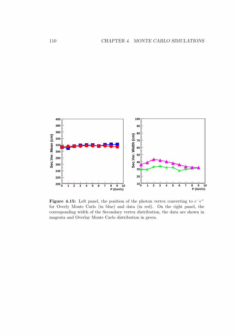
110 CHAPTER 4. MONTE CARLO SIMULATIONS
P (GeV/c)0 1 2 3 4 5 6 7 8 9 10
Sec
.Ver
. Wid
th (
cm)
10
20
30
40
50
60
70
80
90
100
P (GeV/c)0 1 2 3 4 5 6 7 8 9 10
Sec
.Ver
. Mea
n (
cm)
200
220
240
260
280
300
320
340
360
380
400
Figure 4.15: Left panel, the position of the photon vertex converting to e−e+
for Overly Monte Carlo (in blue) and data (in red). On the right panel, thecorresponding width of the Secondary vertex distribution, the data are shown inmagenta and Overlay Monte Carlo distribution in green.

4.8. ACCEPTANCE AND EFFICIENCY EVALUATION 111
pi0-invMass-test3-y00-pt00
Entries -2777Mean 0.3632RMS 0.1034
(GeV)γ γInv.Mass 0 0.2 0.4
Sig
nal
=S-N
.M
-200
-150
-100
-50
0
50
100
The invariant mass pi0-invMass-test3-y00-pt01
Entries -4268Mean 0.2835RMS 0.1349
(GeV)γ γInv.Mass 0 0.2 0.4
Sig
nal
=S-N
.M
-200
0
200
400
600
800
1000
The invariant mass
pi0-invMass-test3-y00-pt02
Entries 3025Mean 0.2049RMS 0.1155
(GeV)γ γInv.Mass 0 0.2 0.4
Sig
nal
=S-N
.M
0
500
1000
1500
2000
The invariant mass pi0-invMass-test3-y00-pt03
Entries 3799Mean 0.1972RMS 0.1105
(GeV)γ γInv.Mass 0 0.2 0.4
Sig
nal
=S-N
.M
-200
0
200
400
600
800
1000
1200
1400
The invariant mass
pi0-invMass-test3-y00-pt04
Entries 354Mean 0.2021RMS 0.1078
(GeV)γ γInv.Mass 0 0.2 0.4
Sig
nal
=S-N
.M
-100
0
100
200
300
400
500
600
700
The invariant mass pi0-invMass-test3-y00-pt05
Entries 1120Mean 0.2198RMS 0.1137
(GeV)γ γInv.Mass 0 0.2 0.4
Sig
nal
=S-N
.M
-50
0
50
100
150
200
250
The invariant mass
pi0-invMass-test3-y00-pt06
Entries 337Mean 0.2474RMS 0.129
(GeV)γ γInv.Mass 0 0.2 0.4
Sig
nal
=S-N
.M
-20
0
20
40
60
80
The invariant mass
(GeV)γ γInv.Mass 0 0.2 0.4
Sig
nal
=S-N
.M
-5
0
5
10
15
20
25
The invariant mass
Figure 4.16: The Mean and Width of the Secondary vertex.

112 CHAPTER 4. MONTE CARLO SIMULATIONS
pi0-invMass-test3-y01-pt00
Entries -3345Mean 0.3451RMS 0.108
(GeV)γ γInv.Mass 0 0.2 0.4
Sig
nal
=S-N
.M
-200
-150
-100
-50
0
50
100
The invariant mass pi0-invMass-test3-y01-pt01
Entries 2435Mean 0.2566RMS 0.1278
(GeV)γ γInv.Mass 0 0.2 0.4
Sig
nal
=S-N
.M
-200
0
200
400
600
800
1000
The invariant mass
pi0-invMass-test3-y01-pt02
Entries 4675Mean 0.204RMS 0.1112
(GeV)γ γInv.Mass 0 0.2 0.4
Sig
nal
=S-N
.M
-200
0
200
400
600
800
1000
1200
1400
1600
1800
The invariant mass pi0-invMass-test3-y01-pt03
Entries 3415Mean 0.1857RMS 0.1014
(GeV)γ γInv.Mass 0 0.2 0.4
Sig
nal
=S-N
.M
-200
0
200
400
600
800
1000
1200
1400
1600
The invariant mass
pi0-invMass-test3-y01-pt04
Entries 2083Mean 0.1997RMS 0.1153
(GeV)γ γInv.Mass 0 0.2 0.4
Sig
nal
=S-N
.M
-100
0
100
200
300
400
500
600
The invariant mass pi0-invMass-test3-y01-pt05
Entries 166Mean 0.2373RMS 0.1305
(GeV)γ γInv.Mass 0 0.2 0.4
Sig
nal
=S-N
.M
-50
0
50
100
150
200
The invariant mass
pi0-invMass-test3-y01-pt06
Entries 123Mean 0.2513RMS 0.1172
(GeV)γ γInv.Mass 0 0.2 0.4
Sig
nal
=S-N
.M
-20
0
20
40
60
The invariant mass
(GeV)γ γInv.Mass 0 0.2 0.4
Sig
nal
=S-N
.M
-10
-5
0
5
10
15
20
25
30
The invariant mass
Figure 4.17: The Mean and Width of the Secondary vertex.

4.8. ACCEPTANCE AND EFFICIENCY EVALUATION 113
(GeV)γ γInv.Mass 0 0.2 0.4
Sig
nal
=S-N
.M
-60
-40
-20
0
20
40
60
80
The invariant mass
(GeV)γ γInv.Mass 0 0.2 0.4
Sig
nal
=S-N
.M
-60
-40
-20
0
20
40
60
80
100
120
The invariant mass
(GeV)γ γInv.Mass 0 0.2 0.4
Sig
nal
=S-N
.M
-80
-60
-40
-20
0
20
40
60
80
100
The invariant mass
(GeV)γ γInv.Mass 0 0.2 0.4
Sig
nal
=S-N
.M
-50
0
50
100
150
200
The invariant mass
(GeV)γ γInv.Mass 0 0.2 0.4
Sig
nal
=S-N
.M
-20
0
20
40
60
The invariant mass
(GeV)γ γInv.Mass 0 0.2 0.4
Sig
nal
=S-N
.M
-10
0
10
20
30
The invariant mass
(GeV)γ γInv.Mass 0 0.2 0.4
Sig
nal
=S-N
.M
-4
-2
0
2
4
6
8
10
12
The invariant mass
(GeV)γ γInv.Mass 0 0.2 0.4
Sig
nal
=S-N
.M
-2
0
2
4
6
8
The invariant mass
Figure 4.18: The Mean and Width of the Secondary vertex.

114 CHAPTER 4. MONTE CARLO SIMULATIONS
(GeV/c)tP0 0.2 0.4 0.6 0.8 1 1.2 1.4 1.6 1.8
)2M
ean
(G
eV/c
0.1
0.12
0.14
0.16
0.18
0.2
(GeV/c)tP0 0.2 0.4 0.6 0.8 1 1.2 1.4 1.6 1.8
)2M
ean
(G
eV/c
0.1
0.12
0.14
0.16
0.18
0.2
(GeV/c)tP0 0.2 0.4 0.6 0.8 1 1.2 1.4 1.6 1.8
)2M
ean
(G
eV/c
0.1
0.12
0.14
0.16
0.18
0.2
Figure 4.19: The Mean and Width of the Secondary vertex.

4.8. ACCEPTANCE AND EFFICIENCY EVALUATION 115
(GeV/c)tP0 0.2 0.4 0.6 0.8 1 1.2 1.4 1.6 1.8
)2W
idth
(M
eV/c
0
0.005
0.01
0.015
0.02
0.025
0.03
0.035
0.04
(GeV/c)tP0 0.2 0.4 0.6 0.8 1 1.2 1.4 1.6 1.8
)2W
idth
(M
eV/c
0
0.005
0.01
0.015
0.02
0.025
0.03
0.035
0.04
(GeV/c)tP0 0.2 0.4 0.6 0.8 1 1.2 1.4 1.6 1.8
)2W
idth
(M
eV/c
0
0.005
0.01
0.015
0.02
0.025
0.03
0.035
0.04
Figure 4.20: The Mean and Width of the Secondary vertex.

116 CHAPTER 4. MONTE CARLO SIMULATIONS
(GeV/c)t
p0 0.2 0.4 0.6 0.8 1 1.2 1.4 1.6 1.8 2
Acc
epta
nce
0.1
0.2
0.3
0.4
0.5
0.6
0.7
0.8
0.9
Figure 4.21: The acceptance of the neutral pion as function of rapidity andtransverse momentum.

4.8. ACCEPTANCE AND EFFICIENCY EVALUATION 117
(GeV/c)t
p
0 0.2 0.4 0.6 0.8 1 1.2 1.4 1.6 1.8 2
Rec
. Eff
icie
ncy
-610
-510
-410
y < 2.4≤2.2
y < 2.6≤2.4
y < 2.7≤2.6
Figure 4.22: The reconstruction efficiencies distributions versus the π0 transversemomentum studied for different rapidity bins.

118 CHAPTER 4. MONTE CARLO SIMULATIONS

5Results
119


Bibliography
[1] T. P. Cheng and L. F. Li. Gauge theory of elementary particle physics:Problems and solutions. Oxford, UK: Clarendon (2000) 306 p.
[2] Chen-Ning Yang and Robert L. Mills. Conservation of isotopic spin andisotopic gauge invaria
[3] J. Podolanski and R. Armenteros: Analysis of V-Events, Phil. Mag. 45(1954) 13-30.nce. Phys. Rev., 96:191–195, 1954.
[4] T. Muta. Foundations of Quantum Chromodynamics. World ScientificPublishing, 1987.
[5] D.V. Schroder M.E, Peskin. An Introduction to Quantum Field Theory.Addison-Wesley, New York, 1995.
[6] Siegfried Bethke. alpha(s) 2002. Nucl. Phys. Proc. Suppl., 121:74–81,2003.
[7] M. Luscher, K. Symanzik, and P. Weisz. Anomalies of the Free LoopWave Equation in the WKB Approximation. Nucl. Phys., B173:365,1980.
[8] J. Engels, F. Karsch, and H. Satz. A finite size analysis of the heavyquark potential in deconfining medium. Nucl. Phys., B315:419, 1989.
[9] V. Bornyakov et al. Heavy quark potential in lattice QCD at finitetemperature. 2003.
[10] Edward V. Shuryak. Quark-Gluon Plasma and Hadronic Production ofLeptons, Photons and Psions. Phys. Lett., B78:150, 1978.
[11] A. Andronic, P. Braun-Munzinger, and J. Stachel. Hadron productionin central nucleus nucleus collisions at chemical freeze-out. Nucl. Phys.,A772:167–199, 2006.
[12] Bertrand C. Barrois. Superconducting Quark Matter. Nucl. Phys.,B129:390, 1977.
121

122 BIBLIOGRAPHY
[13] John B. Kogut. The lattice gauge theory approach to quantum chromo-dynamics. Rev. Mod. Phys., 55(3):775–836, Jul 1983.
[14] Frithjof Karsch. Lattice results on QCD thermodynamics. Nucl. Phys.,A698:199–208, 2002.
[15] P.Holl et al. CERN/SPSLC 91-1. The quark-hadron transition in cos-mology and astrophysics. CERN-SPSLC.
[16] G. Agakishiev et al. First results from the CERES radial TPC. Nucl.Phys., A661:673–676, 1999.
[17] E. Gatti and P. Rehak. Semiconductor drift chamber - an application ofa novel charge transport scheme. Nucl. Instrum. Meth., A225:608–614,1984.
[18] Diploma Thesis O. Nix. Foundations of Quantum Chromodynamics.Universitat Heidelberg, 1996.
[19] C. Amsler et al. Review of particle physics. Phys. Lett., B667:1, 2008.
[20] J. Podolanski and R. Armenteros. Analysis of v-events. Phil. Mag.,45:13–30, 1954.
[21] R. Brun and F. Rademakers. ROOT: An object oriented data analysisframework. Nucl. Instrum. Meth., A389:81–86, 1997.
[22] Johanna Stachel. Towards the quark-gluon plasma. Nucl. Phys.,A654:119c–135c, 1999.
[23] C. Hohne. Strangeness production in nuclear collisions: Recent resultsfrom experiment NA49. Nucl. Phys., A661:485–488, 1999.
[24] et al. Afanasiev. Energy dependence of pion and kaon production incentral pb+pb collisions. Phys. Rev. C, 66(5):054902, Nov 2002.
[25] P. Braun-Munzinger, I. Heppe, and J. Stachel. Chemical equilibrationin Pb + Pb collisions at the SPS. Phys. Lett., B465:15–20, 1999.
[26] R Brun, F Bruyant, M Maire, A C McPherson, and P Zanarini. GEANT3: user’s guide Geant 3.10, Geant 3.11; rev. version. CERN, Geneva,1987.