100

§Chapter 5

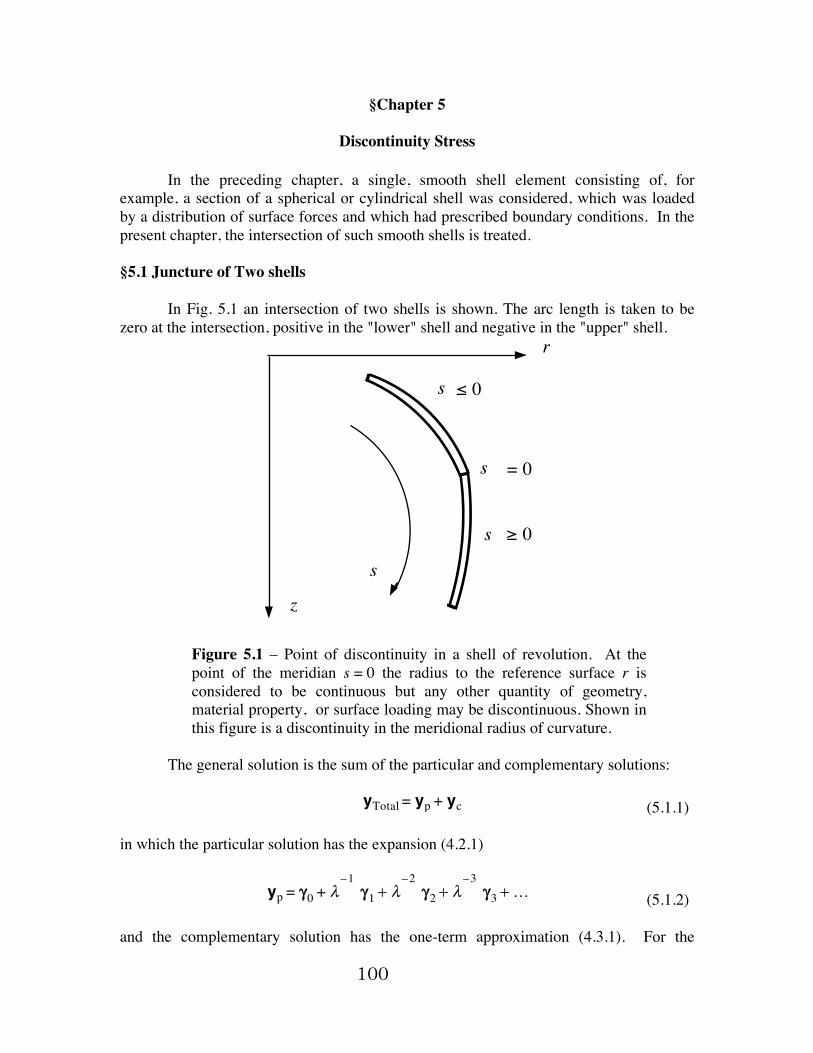
Discontinuity Stress In the preceding chapter, a single, smooth shell element consisting of, for example, a section of a spherical or cylindrical shell was considered, which was loaded by a distribution of surface forces and which had prescribed boundary conditions. In the present chapter, the intersection of such smooth shells is treated. §5.1 Juncture of Two shells In Fig. 5.1 an intersection of two shells is shown. The arc length is taken to be zero at the intersection, positive in the "lower" shell and negative in the "upper" shell.

s

s

s

s

= 0

≤ 0

≥ 0

r

z

Figure 5.1 – Point of discontinuity in a shell of revolution. At the point of the meridian s = 0 the radius to the reference surface r is considered to be continuous but any other quantity of geometry, material property, or surface loading may be discontinuous. Shown in this figure is a discontinuity in the meridional radius of curvature.

The general solution is the sum of the particular and complementary solutions: yTotal = yp + yc (5.1.1) in which the particular solution has the expansion (4.2.1)

yp = γ0 + λ–1

γ1 + λ–2

γ2 + λ–3

γ3 + ... (5.1.2) and the complementary solution has the one-term approximation (4.3.1). For the

101

solutions on the two shell segments which decrease with the distance, the one-term approximation is taken from (4.3.9):

yc =Re A eλ ξ α 0 ξ ′, x for x ≤ 0

Re B e– λ ξ α 0 – ξ ′, x for x ≥ 0 (5.1.3)

It is assumed that the distance from the intersection point under consideration to the nearest boundary in the upper and lower shells is greater than the decay distance. If the radial coordinate r is continuous at the intersection point and if no concentrated line loads act at the intersection point, then each element in the vector (4.1.1) or (2.11.23) must be continuous. Thus the total solution must be continuous:

ΔyTotal = yTotal 0 + – yTotal 0 – = Δy c + Δy p = 0 (5.1.4) so the jump in the complementary solution must be the negative of that in the particular solution:

Δyc = – Δyp (5.1.5) It is clear that the magnitude of the stress concentration due to the bending stress of the complementary solution depends on the magnitude of the discontinuity. In the preceding chapter it was found that generally for a shell under, say, pressure loading, clamping the boundary produces stresses in the complementary solution which are the same order of magnitude of those in the particular solution. When the boundary condition is prescribed such that the radial force required by the particular solution cannot be supplied, the stress in the complementary solution is of the order of magnitude of the square root of radius–to–thickness ( λ ) larger. With the expansion (5.1.2) it is possible to obtain a similar classification of the severity of various discontinuities without carrying out specific calculations. The terms in the expansion of the particular solution are given in (4.2.8-10). If a discontinuity in slope of the meridian occurs, the leading term γ0 is discontinuous. Since this term provides the radial resultant H, this is similar to the case of prescribing for the complementary solution a radial force, which produces stresses O (λ ) larger. If the slope is continuous, but the radius of meridional curvature r1 is discontinuous, γ0 is continuous but the term γ1 is discontinuous. This causes the stress in the complementary solution to be O(1), similar to the situation of a clamped edge on the single shell segment. If the geometry is entirely continuous, but the tangential pressure ps is discontinuous, the terms γ0 and γ1 are continuous but γ2 is discontinuous. Therefore the stress due to the complementary solution is small O( λ-1 ). A more complete summary of the effect of the various types of discontinuities is contained in the following table:

102

________________________________________________________________________ Table 5.1 – Effect of discontinuities in a shell of revolution. Particular Solution Complementary Solution Type Discontinuity Causes With Stress concentration in quantity discontinuity physical magnitude in term quantity I φ γ

0 H O( λ ) II r1

γ1 h O(1)

pζ γ1 h O(1)

E γ1 h O(1)

t γ1 h O(1)

ν γ1 h O(1)

III d r1 / ds γ

2 χ O( λ-1 )

d pζ / ds γ2 χ O( λ-1 )

ps γ2 χ O( λ-1 )

d E/ ds γ2 χ O( λ-1 )

d t / ds γ2 χ O( λ-1 )

d ν / ds γ2 χ O( λ-1 ) ________________________________________________________________________ Thus the boundary condition of an edge free from radial constraint can be considered as a special case of the Type I discontinuity, which is severe and to be avoided in a structurally efficient shell structure. The boundary condition of a clamped edge can be considered as a special case of the Type II discontinuity, which is generally unavoidable. The Type III discontinuities are rather benign and for a first approximation can be ignored. For the analysis, one approach is to use the discontinuity conditions on the complementary solution (5.1.5) and form the algebraic equations for the unknown constants A and B in (5.1.6). A better procedure is to make use of the edge stiffness coefficients which can be obtained for each shell separately. To use these for the point of

103

juncture of the two shells it is convenient to partition the vector of variables (2.11.23) into the "force" and "displacement" quantities:

Y = F

D F = r Msr H

D =χh (5.1.6)

The dimensionless variables (4.1.1) may also be used. However, these are helpful in understanding the behavior of a single shell segment. For the interaction of two or more shells fewer mistakes are made if the basic variables are used. The total solution is the sum of the particular and complementary solution (5.1.1) which can be written as

F(1) = Fp(1) + Fc

(1)

D (1) = Dp(1) + Dc

(1)

F(2) = Fp(2) + Fc

(2)

D (2) = Dp(2) + Dc

(2)

(5.1.7-10) in which the superscript (1) indicates the shell for s ≤ 0 and the superscript (2) indicates the shell for s ≥ 0. The continuity condition (5.1.4) is

F(1) = F(2) = FD (1) = D (2) = D (5.1.11-12)

in which the quantities without the superscript denote the total at the intersection. The edge stiffnesses of the two shells are:

Fc(1) = K(1) • D c

(1)

Fc(2) = K(2) • D c

(2) (5.1.13-14)

which with (5.1.7-10) may be rewritten as

F(1) – Fp(1) = K(1) • D (1) – Dp

(1)

F(2) – Fp(2) = K(2) • D (2) – Dp

(2) (5.1.15-16)

Using the continuity condition (5.1.11-12) yields the equation for the total displacement at the intersection:

104

K(1) – K(2) • D = FR(2) – FR(1) (5.1.17) in which

FR(1) = Fp(1) - K(1) • Dp

(1)

FR(2) = Fp(2) - K(2) • Dp

(2) (5.1.18-19)

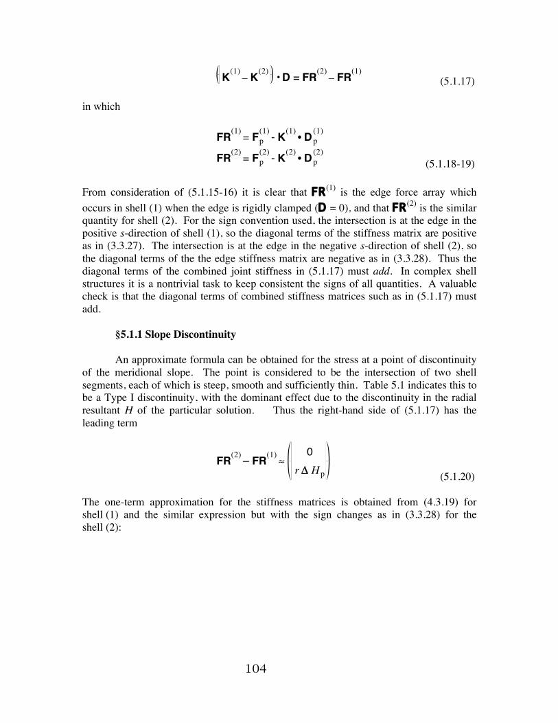
From consideration of (5.1.15-16) it is clear that FR (1) is the edge force array which occurs in shell (1) when the edge is rigidly clamped (D = 0), and that FR (2) is the similar quantity for shell (2). For the sign convention used, the intersection is at the edge in the positive s-direction of shell (1), so the diagonal terms of the stiffness matrix are positive as in (3.3.27). The intersection is at the edge in the negative s-direction of shell (2), so the diagonal terms of the the edge stiffness matrix are negative as in (3.3.28). Thus the diagonal terms of the combined joint stiffness in (5.1.17) must add. In complex shell structures it is a nontrivial task to keep consistent the signs of all quantities. A valuable check is that the diagonal terms of combined stiffness matrices such as in (5.1.17) must add. §5.1.1 Slope Discontinuity An approximate formula can be obtained for the stress at a point of discontinuity of the meridional slope. The point is considered to be the intersection of two shell segments, each of which is steep, smooth and sufficiently thin. Table 5.1 indicates this to be a Type I discontinuity, with the dominant effect due to the discontinuity in the radial resultant H of the particular solution. Thus the right-hand side of (5.1.17) has the leading term

FR(2) – FR(1) ≈

0r Δ Hp (5.1.20)

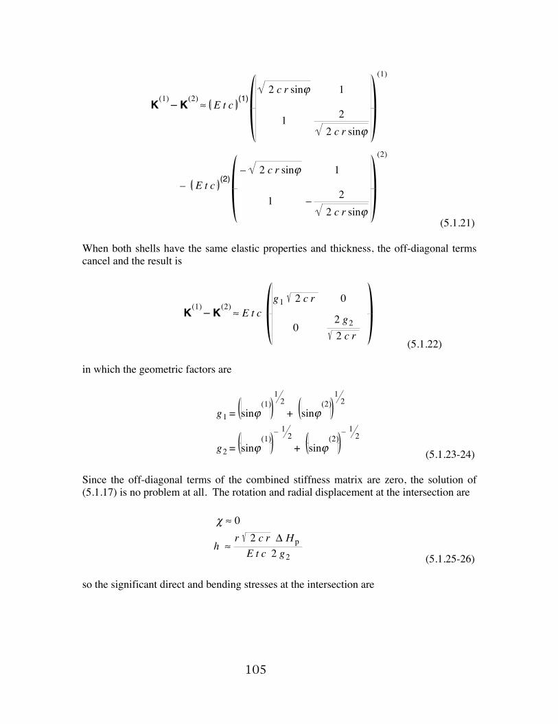
The one-term approximation for the stiffness matrices is obtained from (4.3.19) for shell (1) and the similar expression but with the sign changes as in (3.3.28) for the shell (2):

105

K(1) – K(2) ≈ E t c(1)

2 c r sinϕ 1

1 22 c r sinϕ

(1)

– E t c(2)

– 2 c r sinϕ 1

1 – 22 c r sinϕ

(2)

(5.1.21) When both shells have the same elastic properties and thickness, the off-diagonal terms cancel and the result is

K(1) – K(2) ≈ E t cg1 2 c r 0

02 g22 c r

(5.1.22) in which the geometric factors are

g1 = sinϕ(1)

12+ sinϕ

(2)12

g2 = sinϕ(1)

– 1 2+ sinϕ

(2)– 1 2

(5.1.23-24) Since the off-diagonal terms of the combined stiffness matrix are zero, the solution of (5.1.17) is no problem at all. The rotation and radial displacement at the intersection are

χ ≈ 0

h ≈r 2 c r Δ HpE t c 2 g2 (5.1.25-26)

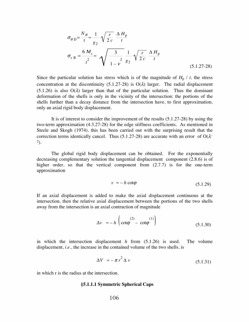
so the significant direct and bending stresses at the intersection are

106

σθ D=N θt ≈

1

g2

r2 c

Δ Hpt

σs B =6Μ s

t2≈

3

1 – ν2

1

g2

r2 c

Δ Hpt

(5.1.27-28) Since the particular solution has stress which is of the magnitude of Hp / t, the stress concentration at the discontinuity (5.1.27-28) is O(λ) larger. The radial displacement (5.1.26) is also O(λ) larger than that of the particular solution. Thus the dominant deformation of the shells is only in the vicinity of the intersection; the portions of the shells further than a decay distance from the intersection have, to first approximation, only an axial rigid body displacement. It is of interest to consider the improvement of the results (5.1.27-28) by using the two-term approximation (4.3.27-28) for the edge stiffness coefficients. As mentioned in Steele and Skogh (1974), this has been carried out with the surprising result that the correction terms identically cancel. Thus (5.1.27-28) are accurate with an error of O(λ–2). The global rigid body displacement can be obtained. For the exponentially decreasing complementary solution the tangential displacement component (2.8.6) is of higher order, so that the vertical component from (2.7.7) is for the one-term approximation

v ≈ – h cotϕ (5.1.29) If an axial displacement is added to make the axial displacement continuous at the intersection, then the relative axial displacement between the portions of the two shells away from the intersection is an axial contraction of magnitude

Δv ≈ – h cotϕ(2)– cotϕ

(1)

(5.1.30) in which the intersection displacement h from (5.1.26) is used. The volume displacement, i.e., the increase in the contained volume of the two shells, is

ΔV ≈ – π r2 Δ v (5.1.31) in which r is the radius at the intersection. §5.1.1.1 Symmetric Spherical Caps

107

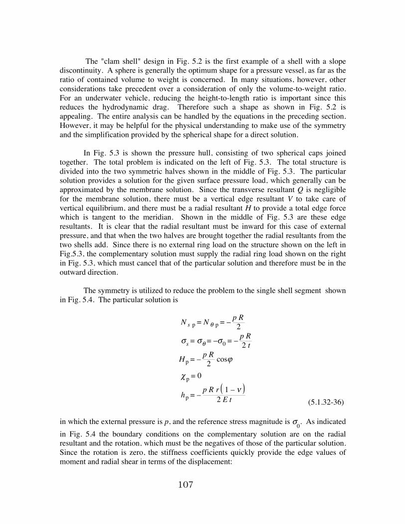
The "clam shell" design in Fig. 5.2 is the first example of a shell with a slope discontinuity. A sphere is generally the optimum shape for a pressure vessel, as far as the ratio of contained volume to weight is concerned. In many situations, however, other considerations take precedent over a consideration of only the volume-to-weight ratio. For an underwater vehicle, reducing the height-to-length ratio is important since this reduces the hydrodynamic drag. Therefore such a shape as shown in Fig. 5.2 is appealing. The entire analysis can be handled by the equations in the preceding section. However, it may be helpful for the physical understanding to make use of the symmetry and the simplification provided by the spherical shape for a direct solution. In Fig. 5.3 is shown the pressure hull, consisting of two spherical caps joined together. The total problem is indicated on the left of Fig. 5.3. The total structure is divided into the two symmetric halves shown in the middle of Fig. 5.3. The particular solution provides a solution for the given surface pressure load, which generally can be approximated by the membrane solution. Since the transverse resultant Q is negligible for the membrane solution, there must be a vertical edge resultant V to take care of vertical equilibrium, and there must be a radial resultant H to provide a total edge force which is tangent to the meridian. Shown in the middle of Fig. 5.3 are these edge resultants. It is clear that the radial resultant must be inward for this case of external pressure, and that when the two halves are brought together the radial resultants from the two shells add. Since there is no external ring load on the structure shown on the left in Fig.5.3, the complementary solution must supply the radial ring load shown on the right in Fig. 5.3, which must cancel that of the particular solution and therefore must be in the outward direction. The symmetry is utilized to reduce the problem to the single shell segment shown in Fig. 5.4. The particular solution is

N s p = N θ p = –p R2

σs = σθ = –σ0 = –p R2 t

Hp = –p R2 cosϕ

χ p = 0

hp = –p R r 1 – ν

2 E t (5.1.32-36) in which the external pressure is p, and the reference stress magnitude is σ

0. As indicated

in Fig. 5.4 the boundary conditions on the complementary solution are on the radial resultant and the rotation, which must be the negatives of those of the particular solution. Since the rotation is zero, the stiffness coefficients quickly provide the edge values of moment and radial shear in terms of the displacement:

108

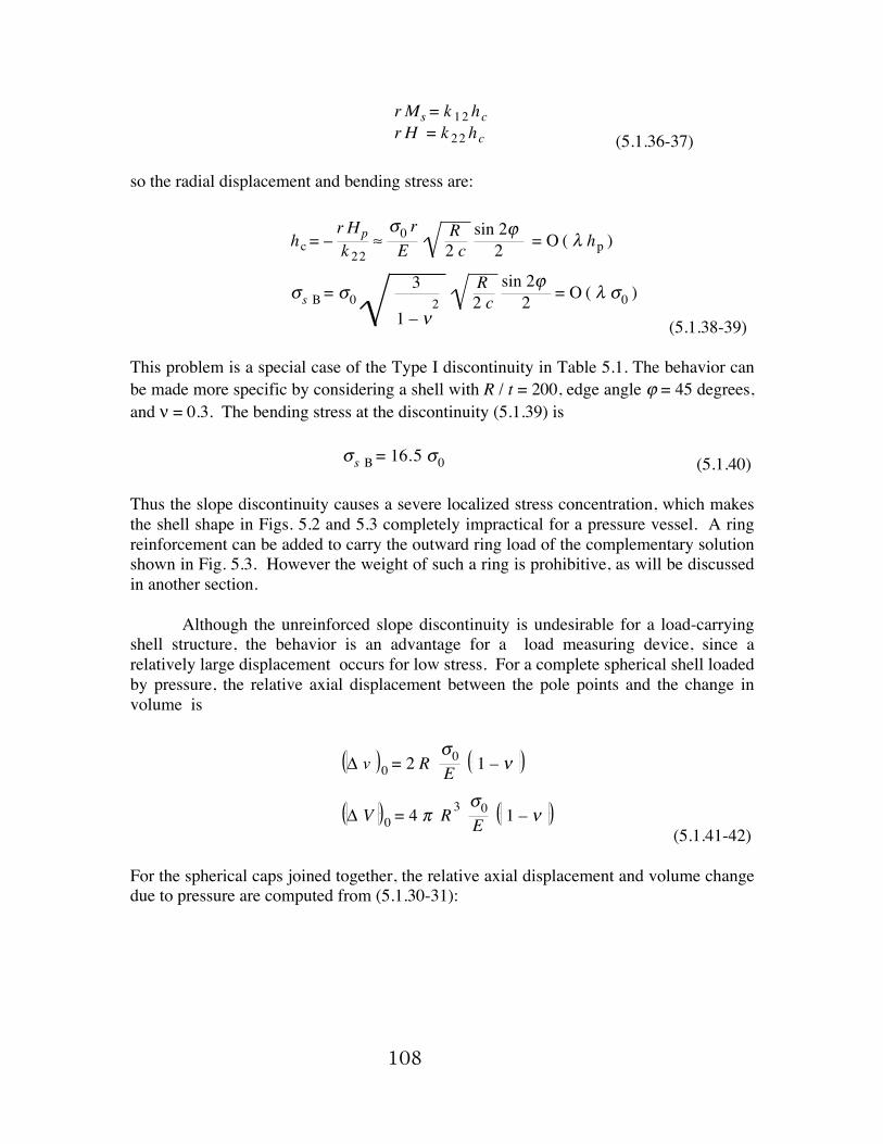
r Ms = k 12 hcr H = k 22 hc (5.1.36-37)

so the radial displacement and bending stress are:

hc = –r Hpk 22

≈σ0 rE

R2 c

sin 2ϕ2 = O ( λ hp )

σs B = σ03

1 – ν2

R2 c

sin 2ϕ2 = O ( λ σ0 )

(5.1.38-39) This problem is a special case of the Type I discontinuity in Table 5.1. The behavior can be made more specific by considering a shell with R / t = 200, edge angle ϕ = 45 degrees, and ν = 0.3. The bending stress at the discontinuity (5.1.39) is

σs B = 16.5 σ0 (5.1.40) Thus the slope discontinuity causes a severe localized stress concentration, which makes the shell shape in Figs. 5.2 and 5.3 completely impractical for a pressure vessel. A ring reinforcement can be added to carry the outward ring load of the complementary solution shown in Fig. 5.3. However the weight of such a ring is prohibitive, as will be discussed in another section. Although the unreinforced slope discontinuity is undesirable for a load-carrying shell structure, the behavior is an advantage for a load measuring device, since a relatively large displacement occurs for low stress. For a complete spherical shell loaded by pressure, the relative axial displacement between the pole points and the change in volume is

Δ v 0 = 2 Rσ0E 1 – ν

Δ V 0 = 4 π R 3σ0E 1 – ν

(5.1.41-42) For the spherical caps joined together, the relative axial displacement and volume change due to pressure are computed from (5.1.30-31):

109

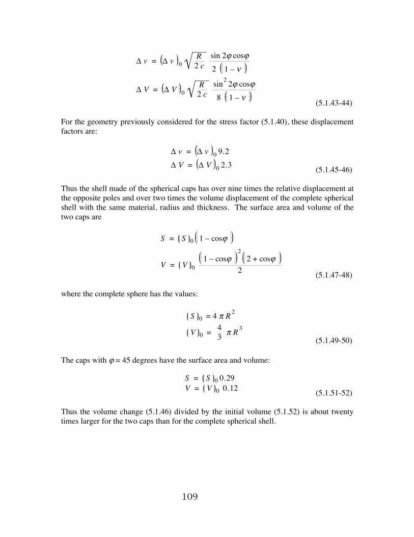
Δ v = Δ v 0R2 c

sin 2ϕ cosϕ2 1 – ν

Δ V = Δ V 0R2 c

sin2 2ϕ cosϕ8 1 – ν (5.1.43-44)

For the geometry previously considered for the stress factor (5.1.40), these displacement factors are:

Δ v = Δ v 0 9.2Δ V = Δ V 0 2.3 (5.1.45-46)

Thus the shell made of the spherical caps has over nine times the relative displacement at the opposite poles and over two times the volume displacement of the complete spherical shell with the same material, radius and thickness. The surface area and volume of the two caps are

S = S 0 1 – cosϕ

V = V 01 – cosϕ

22 + cosϕ

2 (5.1.47-48) where the complete sphere has the values:

S 0 = 4 π R2

V 0 =43 π R 3

(5.1.49-50) The caps with ϕ = 45 degrees have the surface area and volume:

S = S 0 0.29V = V 0 0.12 (5.1.51-52)

Thus the volume change (5.1.46) divided by the initial volume (5.1.52) is about twenty times larger for the two caps than for the complete spherical shell.

110

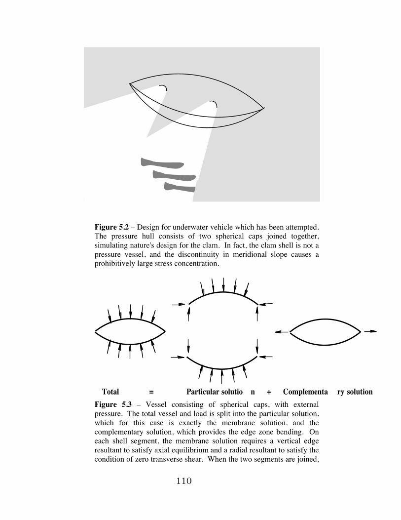
Figure 5.2 – Design for underwater vehicle which has been attempted. The pressure hull consists of two spherical caps joined together, simulating nature's design for the clam. In fact, the clam shell is not a pressure vessel, and the discontinuity in meridional slope causes a prohibitively large stress concentration.

Total = Particular solutio n + Complementa ry solutionFigure 5.3 – Vessel consisting of spherical caps, with external pressure. The total vessel and load is split into the particular solution, which for this case is exactly the membrane solution, and the complementary solution, which provides the edge zone bending. On each shell segment, the membrane solution requires a vertical edge resultant to satisfy axial equilibrium and a radial resultant to satisfy the condition of zero transverse shear. When the two segments are joined,

111

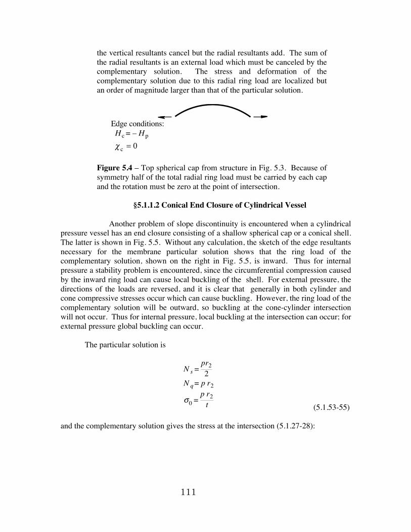
the vertical resultants cancel but the radial resultants add. The sum of the radial resultants is an external load which must be canceled by the complementary solution. The stress and deformation of the complementary solution due to this radial ring load are localized but an order of magnitude larger than that of the particular solution.

Edge conditions:H c = – Hp

χ c = 0 Figure 5.4 – Top spherical cap from structure in Fig. 5.3. Because of symmetry half of the total radial ring load must be carried by each cap and the rotation must be zero at the point of intersection.

§5.1.1.2 Conical End Closure of Cylindrical Vessel Another problem of slope discontinuity is encountered when a cylindrical pressure vessel has an end closure consisting of a shallow spherical cap or a conical shell. The latter is shown in Fig. 5.5. Without any calculation, the sketch of the edge resultants necessary for the membrane particular solution shows that the ring load of the complementary solution, shown on the right in Fig. 5.5, is inward. Thus for internal pressure a stability problem is encountered, since the circumferential compression caused by the inward ring load can cause local buckling of the shell. For external pressure, the directions of the loads are reversed, and it is clear that generally in both cylinder and cone compressive stresses occur which can cause buckling. However, the ring load of the complementary solution will be outward, so buckling at the cone-cylinder intersection will not occur. Thus for internal pressure, local buckling at the intersection can occur; for external pressure global buckling can occur. The particular solution is

N s =pr22

N q= p r2

σ0 =p r2t (5.1.53-55)

and the complementary solution gives the stress at the intersection (5.1.27-28):

112

σθ D= – σ0cosϕ1sinϕ

+ 1

r2 c

σs Β= σθ D3

1 – ν2

(5.1.56-57) in which the angle ϕ is that for the cone. Just as for the spherical caps joined together, the cone-cylinder intersection causes large local stress and displacement.

Total = Particular solutio n + Complementa ry solution Figure 5.5 – Conical end closure on cylindrical pressure vessel. For the internal pressure shown, the radial resultant of the membrane particular solution is outward for the cone and zero for the cylinder. The ring load for the complementary solution, which causes the dominant stress and deformation is therefore inward. Stability is a concern for this case of internal pressure. For external pressure, the ring load is outward, so that buckling in the region of the intersection will not occur.

§5.1.1.3 Cylindrical Pipe in a Dome-Shaped Vessel In Fig. 5.6 is shown a common problem of a cylindrical pipe joined to a vessel which could be spherical, elliptical, or parabolic. The particular solution is straight-forward and the complementary solution causes the stress and displacement at the intersection given by (5.1.25-28). The sketch in Fig. 5.6 shows the important feature that the ring load of the complementary solution is outward for internal pressure. Thus the dominant stress is at the juncture, consisting of circumferential tension and meridional bending stress which causes tension on the outer surface. For external pressure, the

113

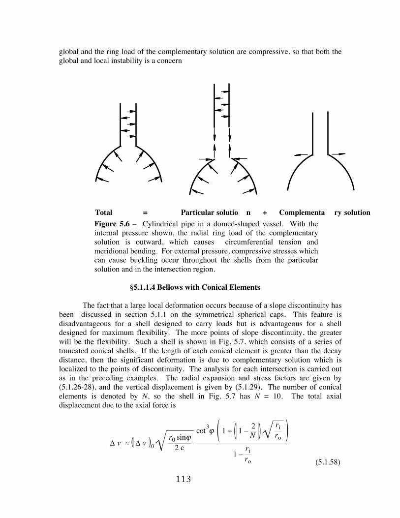
global and the ring load of the complementary solution are compressive, so that both the global and local instability is a concern

Total = Particular solutio n + Complementa ry solution Figure 5.6 – Cylindrical pipe in a domed-shaped vessel. With the internal pressure shown, the radial ring load of the complementary solution is outward, which causes circumferential tension and meridional bending. For external pressure, compressive stresses which can cause buckling occur throughout the shells from the particular solution and in the intersection region.

§5.1.1.4 Bellows with Conical Elements The fact that a large local deformation occurs because of a slope discontinuity has been discussed in section 5.1.1 on the symmetrical spherical caps. This feature is disadvantageous for a shell designed to carry loads but is advantageous for a shell designed for maximum flexibility. The more points of slope discontinuity, the greater will be the flexibility. Such a shell is shown in Fig. 5.7, which consists of a series of truncated conical shells. If the length of each conical element is greater than the decay distance, then the significant deformation is due to complementary solution which is localized to the points of discontinuity. The analysis for each intersection is carried out as in the preceding examples. The radial expansion and stress factors are given by (5.1.26-28), and the vertical displacement is given by (5.1.29). The number of conical elements is denoted by N, so the shell in Fig. 5.7 has N = 10. The total axial displacement due to the axial force is

Δ v ≈ Δ v 0r0 sinϕ2 c

cot3ϕ 1 + 1 – 2Nriro

1 –riro (5.1.58)

114

in which ri and r0 are the radii at the inner and outer points of discontinuity, and the reference displacement of a cylindrical shell with the same total length L, wall thickness t, and with a radius equal to r0 is

Δ v 0 =

P L2 π r0 E t (5.1.59)

The length is related to the angle and number of elements by

tanϕ = L

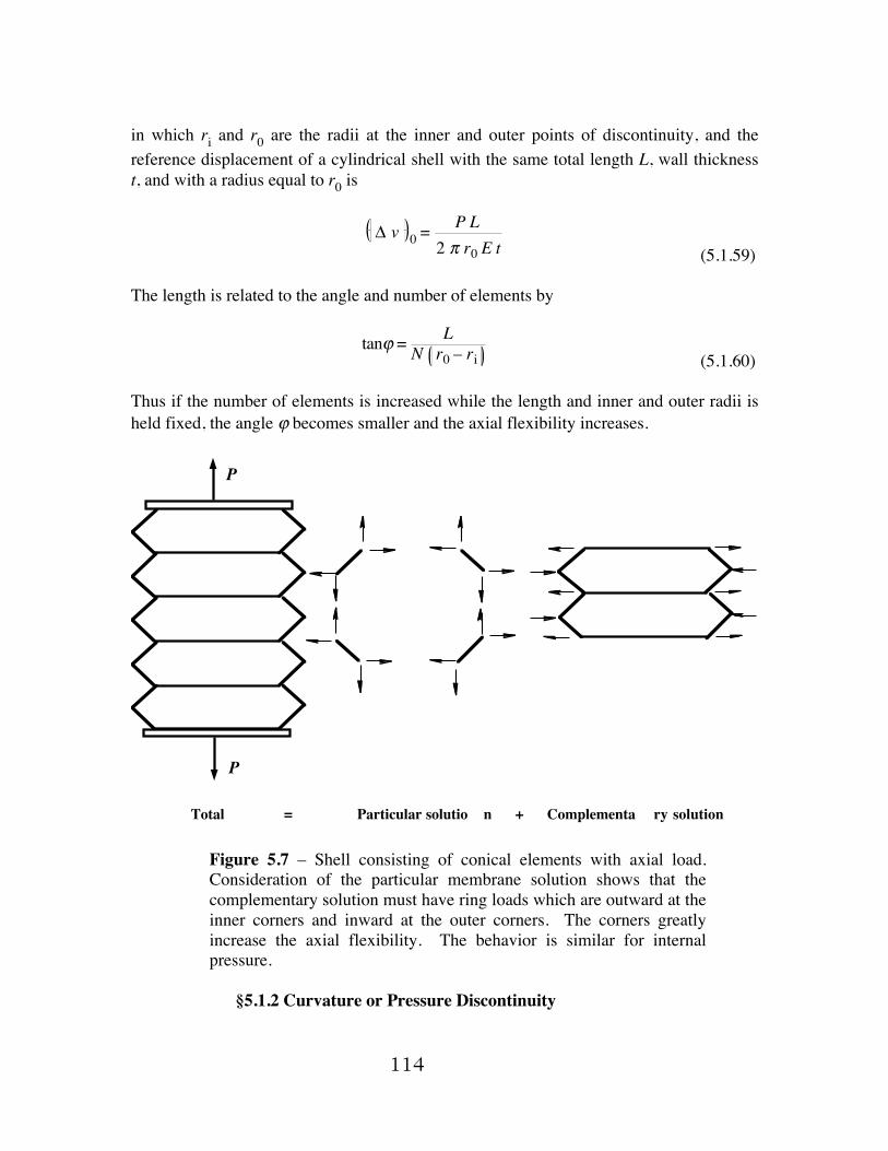
N r0 – ri (5.1.60) Thus if the number of elements is increased while the length and inner and outer radii is held fixed, the angle ϕ becomes smaller and the axial flexibility increases.

Total = Particular solutio n + Complementa ry solution

P

P

Figure 5.7 – Shell consisting of conical elements with axial load. Consideration of the particular membrane solution shows that the complementary solution must have ring loads which are outward at the inner corners and inward at the outer corners. The corners greatly increase the axial flexibility. The behavior is similar for internal pressure.

§5.1.2 Curvature or Pressure Discontinuity

115

If the slope of the meridian is continuous but the curvature is discontinuous, this is classified as Type II in Table 5.1. A similar behavior occurs when the normal pressure component has a discontinuity. The important feature for Type II is that the force discontinuity of the particular solution (5.1.20) is generally negligible. What remains as the most significant terms on the right-hand side of (5.1.17) are

FR(2) – FR(1) ≈ – k12

k22

(2)

hp(2) + k12

k22

(1)

hp(1)

(5.1.61) In the situation that the material properties and thickness are continuous, simple approximate results can be obtained. The one-term approximation for the stiffness coefficients in (5.1.58) and (5.1.17) yield the total displacement and rotation at the intersection, i.e., the solution of (5.1.17):

χ ≈– hp

(2) + hp(1)

2 2 c r sinϕ

h ≈hp(2) + hp

(1)

2 (5.1.62) Thus the total radial displacement is the average of the displacements of the particular solutions from the two shells at the intersection, while the rotation is an order of magnitude larger than that of the particular solutions. For the shell (1) the rotation and displacement of the complementary solution at the edge are:

χ(1)

≈ χ ≈– hp

(2) + hp(1)

2 2 c r sinϕ

hc(1) = h – hp

(1)≈hp(2) – hp

(1)

2 (5.1.63-64) From these the constant A in the solution (5.1.3) is found to have negligible imaginary part, and the bending stress and radial displacement of the complementary solution in the edge zone are

hc(1) = h – hp

(1) e– ξ cosξ

σs B = –Er

3

1 – ν2

h – hp(1) e– ξ sinξ

(5.1.65-66) in which the distance from the edge is normalized to the decay distance:

116

ξ = –s

2 c r2 (5.1.67) The bending stress is zero at the edge and is of maximum amplitude at the point ξ = π /4. §5.1.2.1 Elliptical Head on Cylindrical Vessel An important example of a discontinuity in the meridional curvature is the case shown in Fig. 5.7. The ratio of height to radius at the equator of the ellipse, i.e., the ratio of semi-minor to semi-major axes, is denoted by γ. At the intersection

r2r1=

γ– 2

for ellipse

0 for cylinder (5.1.68) Thus, if the material properties and the thickness of ellipse and cylinder are the same, the discontinuity in the radial displacement of the membrane particular solution is

Δ hp =

p R 2

2 E t γ– 2

(5.1.69) in which the internal pressure is p and the radius of the cylinder is R. The result for the maximum bending stress is obtained from (5.1.66) at the point ξ = π /4, which is

σs B max = 0.293 γ– 2

σs D

σs D=p R2 t (5.1.70-71)

This is a relatively mild stress concentration, in comparison with the Type I discontinuities. The bending stress near the intersection is only 30 % of the meridional membrane stress and 15 % of the circumferential membrane stress in the cylinder for the case of hemispherical head γ = 1. Note, however, that if the height of the head is decreased, γ becomes small, and the circumferential membrane stress in the ellipse and the discontinuity stress become large. In the limit as the height approaches zero and the ellipsoid is a flat plate, the approximate result (5.1.70) is not valid, although the trend to excessively high stress is correct. If the cylinder is twice as thick as the ellipsoid, so that the maximum membrane stress is nearly the same in ellipse and cylinder, the bending stress factor is

117

σs B max = σs D γ

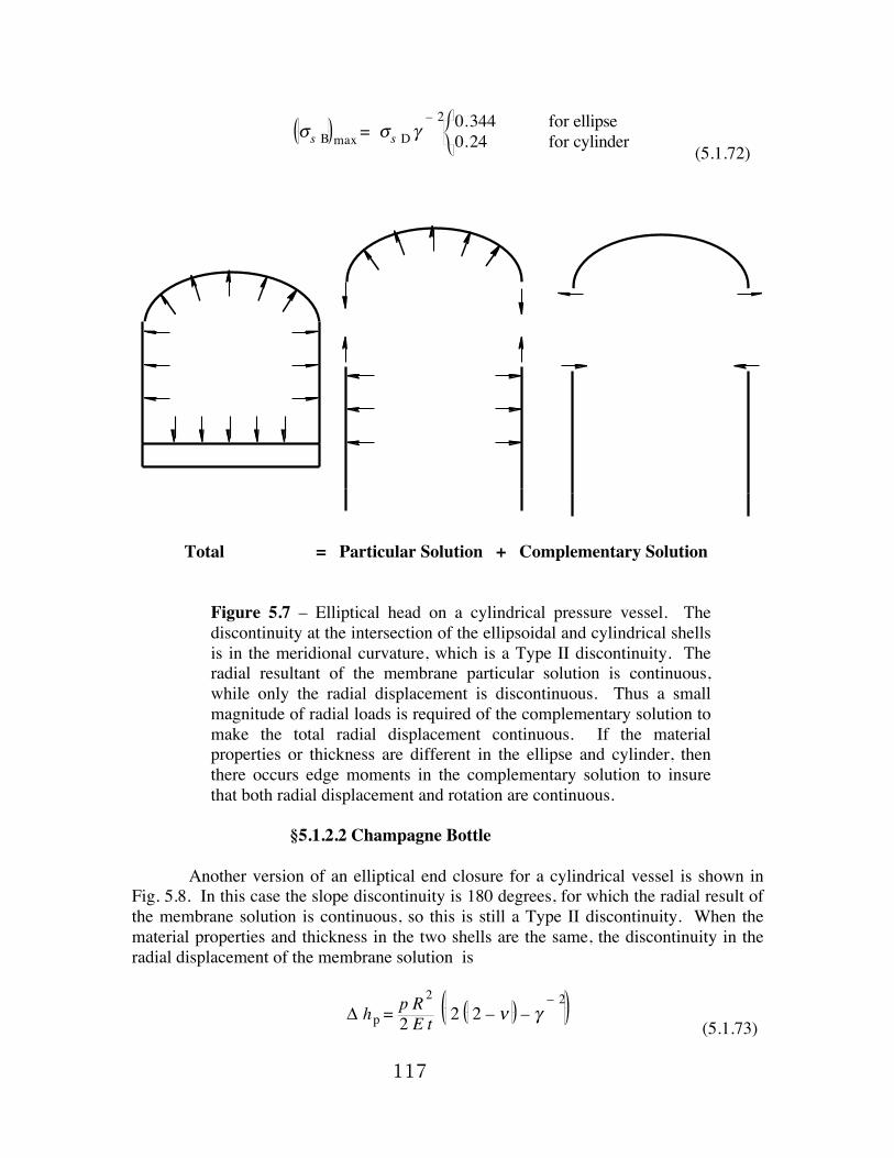
– 2 0.344 for ellipse0.24 for cylinder (5.1.72)

Total = Particular Solution + Complementary Solution

Figure 5.7 – Elliptical head on a cylindrical pressure vessel. The discontinuity at the intersection of the ellipsoidal and cylindrical shells is in the meridional curvature, which is a Type II discontinuity. The radial resultant of the membrane particular solution is continuous, while only the radial displacement is discontinuous. Thus a small magnitude of radial loads is required of the complementary solution to make the total radial displacement continuous. If the material properties or thickness are different in the ellipse and cylinder, then there occurs edge moments in the complementary solution to insure that both radial displacement and rotation are continuous.

§5.1.2.2 Champagne Bottle Another version of an elliptical end closure for a cylindrical vessel is shown in Fig. 5.8. In this case the slope discontinuity is 180 degrees, for which the radial result of the membrane solution is continuous, so this is still a Type II discontinuity. When the material properties and thickness in the two shells are the same, the discontinuity in the radial displacement of the membrane solution is

Δ hp =

p R 2

2 E t 2 2 – ν – γ– 2

(5.1.73)

118

which is larger than (5.1.69) for the hemisphere ( γ = 1) since the membrane displacements of the two shells are in opposite directions. The maximum bending stress from the complementary solution 5.1.66) is

σs B max = 0.293 2 2 – ν – γ– 2

σs D

σs D=p R2 t (5.1.74-76)

It is interesting that this is a reasonable design for an end closure, as far as the discontinuity stress is concerned, which has an advantage for a wine bottle in that it can stand on the table. During processing, champagne bottles are subjected to substantial internal pressure. The potential instability of the ellipsoid, when the pressure is internal, or the cylinder, when the pressure is external, must of course be taken into consideration. The discontinuity stress is negligible for

γ = 2 2 – ν = 0.56 for ν = 0.3 (5.1.77) In this case the radial displacements of the particular solutions for the two shells are equal and in the same direction.

Total = Particular Solution + Complementary Solution

Figure 5.8 – Inverted elliptical head on a cylindrical pressure vessel. The meridional slope change of 180 degrees does not cause a discontinuity in the radial resultant of the particular solution, so this is a Type II discontinuity.

119

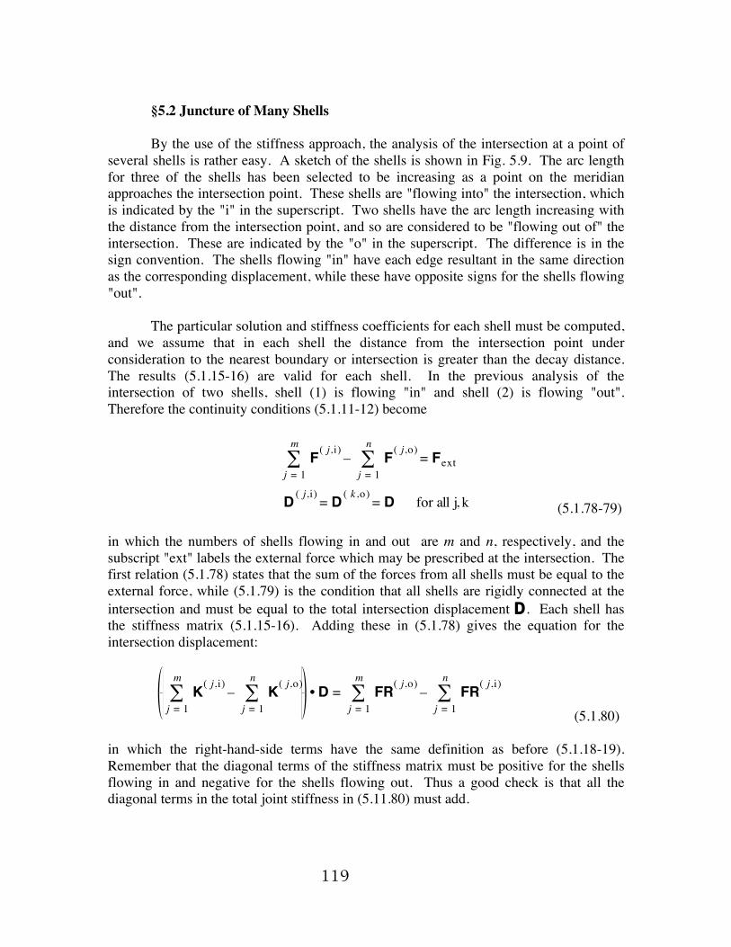
§5.2 Juncture of Many Shells By the use of the stiffness approach, the analysis of the intersection at a point of several shells is rather easy. A sketch of the shells is shown in Fig. 5.9. The arc length for three of the shells has been selected to be increasing as a point on the meridian approaches the intersection point. These shells are "flowing into" the intersection, which is indicated by the "i" in the superscript. Two shells have the arc length increasing with the distance from the intersection point, and so are considered to be "flowing out of" the intersection. These are indicated by the "o" in the superscript. The difference is in the sign convention. The shells flowing "in" have each edge resultant in the same direction as the corresponding displacement, while these have opposite signs for the shells flowing "out". The particular solution and stiffness coefficients for each shell must be computed, and we assume that in each shell the distance from the intersection point under consideration to the nearest boundary or intersection is greater than the decay distance. The results (5.1.15-16) are valid for each shell. In the previous analysis of the intersection of two shells, shell (1) is flowing "in" and shell (2) is flowing "out". Therefore the continuity conditions (5.1.11-12) become

m

∑j = 1

F( j,i) –n

∑j = 1

F( j,o) = Fext

D ( j,i) = D ( k,o) = D for all j, k (5.1.78-79) in which the numbers of shells flowing in and out are m and n, respectively, and the subscript "ext" labels the external force which may be prescribed at the intersection. The first relation (5.1.78) states that the sum of the forces from all shells must be equal to the external force, while (5.1.79) is the condition that all shells are rigidly connected at the intersection and must be equal to the total intersection displacement D . Each shell has the stiffness matrix (5.1.15-16). Adding these in (5.1.78) gives the equation for the intersection displacement:

m

∑j = 1

K( j,i) –n

∑j = 1

K( j,o) • D =m

∑j = 1

FR( j,o) –n

∑j = 1

FR( j,i)

(5.1.80) in which the right-hand-side terms have the same definition as before (5.1.18-19). Remember that the diagonal terms of the stiffness matrix must be positive for the shells flowing in and negative for the shells flowing out. Thus a good check is that all the diagonal terms in the total joint stiffness in (5.11.80) must add.

120

s (1, )i

s (2, )i

s (3, )i

s (1, )o s (2, )o

r

z

Figure 5.9 – The intersection of several shells. Depending on the choice of the direction of increasing arc length, a particular shell is considered to be flowing "into" or "out of" the intersection.