Full Terms & Conditions of access and use can be found athttp://www.tandfonline.com/action/journalInformation?journalCode=ubes20

Download by: [The University of British Columbia] Date: 17 March 2016, At: 11:46

Journal of Business & Economic Statistics

ISSN: 0735-0015 (Print) 1537-2707 (Online) Journal homepage: http://www.tandfonline.com/loi/ubes20

Weak Identification in Fuzzy RegressionDiscontinuity Designs

Donna Feir, Thomas Lemieux & Vadim Marmer

To cite this article: Donna Feir, Thomas Lemieux & Vadim Marmer (2016) Weak Identificationin Fuzzy Regression Discontinuity Designs, Journal of Business & Economic Statistics, 34:2,185-196, DOI: 10.1080/07350015.2015.1024836

To link to this article: http://dx.doi.org/10.1080/07350015.2015.1024836

View supplementary material

Accepted author version posted online: 02Apr 2015.Published online: 17 Mar 2016.

Submit your article to this journal

Article views: 76

View related articles

View Crossmark data

Citing articles: 2 View citing articles

Supplementary materials for this article are available online. Please go to http://tandfonline.com/r/JBES

Weak Identification in Fuzzy RegressionDiscontinuity Designs

Donna FEIRDepartment of Economics, University of Victoria, Victoria, BC, V8W 2Y2, Canada(dfeir@uvic.ca)

Thomas LEMIEUX and Vadim MARMERVancouver School of Economics, University of British Columbia, Vancouver, BC, V6T 1Z1, Canada(thomas.lemieux@ubc.ca; vadim.marmer@ubc.ca)

In fuzzy regression discontinuity (FRD) designs, the treatment effect is identified through a discontinuity inthe conditional probability of treatment assignment. We show that when identification is weak (i.e., whenthe discontinuity is of a small magnitude), the usual t-test based on the FRD estimator and its standarderror suffers from asymptotic size distortions as in a standard instrumental variables setting. This problemcan be especially severe in the FRD setting since only observations close to the discontinuity are usefulfor estimating the treatment effect. To eliminate those size distortions, we propose a modified t-statisticthat uses a null-restricted version of the standard error of the FRD estimator. Simple and asymptoticallyvalid confidence sets for the treatment effect can be also constructed using this null-restricted standarderror. An extension to testing for constancy of the regression discontinuity effect across covariates is alsodiscussed. Supplementary materials for this article are available online.

KEY WORDS: Nonparametric inference; Regression discontinuity design; Treatment effect; Uniformasymptotic size; Weak identification.

1. INTRODUCTION

Since the late 1990s regression discontinuity (RD) and fuzzyregression discontinuity (FRD) designs have been of growingimportance in applied economics. There is extensive theoret-ical work on RD and FRD designs. A few examples includeHahn, Todd, and Van der Klaauw (1999, 2001); Porter (2003);Buddelmeyer and Skoufias (2004); McCrary (2008); Frolich(2007); Frolich and Melly (2008); Otsu, Xu, and Matsushita(2015); Imbens and Kalyanaraman (2012); Calonico, Cattaneo,and Titiunik (2014); Arai and Ichimura (2013); Papay, Willett,and Murnane (2011); Imbens and Zajonc (2011); Dong andLewbel (2010); and Fe (2012). See Van der Klaauw (2008) andLee and Lemieux (2010) for a review of much of this literature.Hundreds of recent applied articles have used RD, and in manycases FRD designs. (For example, as of July 18, 2013, Imbensand Lemieux (2008) review of RD and FRD best practices wascited in 990 articles according to Google Scholar, with 372 ofthese articles explicitly considering FRD.) Around the sametime, the seminal works of Bound, Jaeger, and Baker (1995)and Staiger and Stock (1997) made weak identification in aninstrumental variables (IV) context an important considerationin applied work (see Stock, Wright, and Yogo 2002; Andrewsand Stock 2007 for surveys of the literature). However, despitethe close parallel between an IV setting and the FRD design(see Hahn, Todd, and Van der Klaauw 2001) there has been notheoretical or practical attempt to deal with weak identificationin the FRD design more broadly.

To get a sense of the practical importance of weak iden-tification in the FRD design, we have examined a sample ofinfluential applied articles that use the design. We then apply

the F-statistic standards discussed below to see how many ofthese articles may suffer from a weak identification problem.We find that in about half of the articles where enough informa-tion is reported to compute the F-statistic, weak identificationappears to be a problem in at least one of the empirical spec-ifications. (For the procedure followed to obtain the sample ofarticles, see the online supplement, Section 1.) We take this asevidence that weak identification is a serious concern in theapplied FRD design literature. Since it is a matter of practicalimportance, we examine weak identification in the context of theFRD design, demonstrate the problems that arise, and proposeuniformly valid testing procedures for treatment (RD) effects.

In this article, we show that the local-to-zero analytical frame-work common in the weak instruments literature can be adaptedto FRD, and when identification is weak, we show that the usualt-test based on the FRD estimator and its standard error suffersfrom asymptotic size distortions. The usual confidence inter-vals constructed as estimate ± constant × standard error arealso invalid because their asymptotic coverage probability canbe below the assumed nominal coverage when identification isweak. We rely on novel techniques recently developed in theliterature on uniform size properties of tests and confidence sets(Andrews, Cheng, and Guggenberger 2011) to formally justifyour local-to-zero framework. Unlike the framework used in theweak IV literature, ours depends not only on the sample size butalso on a smoothing parameter (the bandwidth).

© 2016 American Statistical AssociationJournal of Business & Economic Statistics

April 2016, Vol. 34, No. 2DOI: 10.1080/07350015.2015.1024836

185

Dow

nloa

ded

by [

The

Uni

vers

ity o

f B

ritis

h C

olum

bia]

at 1

1:46

17

Mar

ch 2

016

186 Journal of Business & Economic Statistics, April 2016

We suggest a simple modification to the t-test that eliminatesthe asymptotic size distortions caused by weak identification.Unlike the usual t-statistic, the modified t-statistic uses a null-restricted version of the standard error of the FRD estimator.The modified statistic can be used with standard normal criticalvalues for two-sided testing. For two-sided testing, the proposedtest is equivalent to the Anderson–Rubin test (Anderson andRubin 1949) adopted in the weak IV literature (Staiger and Stock1997). For one-sided testing, the modified t-statistic has to beused with nonstandard critical values that must be simulated ona case-by-case basis following the approach of Moreira (2001,2003).

We discuss how to evaluate the magnitude of potential sizedistortions in practice following the approach of Stock and Yogo(2005). The strength of identification is measured by the con-centration parameter, which in the case of FRD depends on themagnitude of the discontinuity in the treatment variable and onthe density of the assignment variable (the variable that deter-mines treatment assignment). The magnitude of potential sizedistortions can be tested by testing hypotheses about the con-centration parameter with noncentral χ2

1 critical values usingthe F-statistic, which is an analog of the first-stage F-statistic inIV regression. Surprisingly, we find critical values that are muchhigher than would be required in a simple IV setting. When theF-statistic is only around 10, which is often used as a thresholdvalue for weak/strong identification in the IV literature, a two-sided test with nominal size of 5% is in fact a 13.6% test, anda 5% one-sided test is in fact a 16.9% test. Nearly zero (under0.5%) size distortions of a 5% two-sided test correspond to thevalues of the F-statistic above 93.

Asymptotically valid confidence sets for the treatment ef-fect can be obtained by inverting tests based on the modi-fied t-statistic. Since the FRD is an exactly identified model,these confidence sets are easy to compute, as their constructiononly involves solving a quadratic equation. Most of the litera-ture on weak instruments deals with the case of over identifiedmodels (see, e.g., Andrews and Stock 2007). In exactly iden-tified models, the approach suggested by Anderson and Rubin(1949) results in efficient inference if instruments turn out tobe strong and remains valid if instruments are weak. However,in over-identified models, Anderson and Rubin’s tests are nolonger efficient even when instruments are strong. Several arti-cles (Kleibergen 2002; Moreira 2003; Andrews, Moreira, andStock 2006) proposed modifications to Anderson and Rubin’sbasic procedure to gain back efficiency in over identified mod-els. Since the FRD design is an exactly identified model, wecan adapt Anderson and Rubin’s approach without any loss ofpower. These confidence sets are expected to be as informativeas the standard ones, when identification is strong. However,unlike the usual confidence intervals, the confidence sets wepropose can be unbounded with positive probability. This prop-erty is expected from valid confidence sets in the situationswith local identification failure and an unbounded parameterspace (see Dufour 1997). In a recent article, Otsu, Xu, and Mat-sushita (2015) proposed empirical likelihood-based inferencefor the RD effect. Using the profile empirical likelihood func-tion, they proposed confidence sets for the RD effect, whichare expected to be robust against weak identification. However,

they did not provide a formal analysis of the weak identifi-cation. While their method does not involve variances estima-tion and for that reason can enjoy better higher-order proper-ties than our approach, it requires computation of the empiricallikelihood function numerically and is computationally moredemanding.

We also discuss testing whether the RD effect is homogenousover differing values of some covariates. The proposed test-ing approach is designed to remain asymptotically valid whenidentification is weak. This is achieved by building a robust con-fidence set for a common RD effect across covariates. The nullhypothesis of the common RD effect is rejected when that con-fidence set is empty.

To illustrate how our proposed confidence sets may differfrom the standard ones in practice, we compare the results ofapplying the standard confidence sets and the proposed confi-dence sets in two separate applications that use the FRD designto estimate the effect of class size on student achievement. Ourmain finding is that, as weak identification becomes more likely,the standard confidence sets and the weak identification robustconfidence sets become increasingly divergent. Interestingly,in a number of cases the robust confidence sets provide moreinformative answers than the standard ones. More generally,the empirical applications, along with a Monte Carlo study re-ported in an online supplement, suggest that our simple androbust procedure for computing confidence sets performs wellwhen identification is either strong or weak.

The rest of the article proceeds as follows. In Section 2, wedescribe the FRD model, derive the uniform asymptotic sizeof usual t-tests for FRD, discuss size distortions and testingfor potential size distortions, and describe weak-identification-robust inference for FRD. Section 3 discusses robust testingfor constancy of the RD effect across covariates. We presentour empirical applications in Section 4. The online supplementcontains additional materials including the proofs and the MonteCarlo results.

2. THEORETICAL RESULTS

2.1 The Model, Estimation, and Standard InferenceApproach

In RD designs, the observed outcome variable yi is modeledas yi = y0i + xiβi , where xi is the treatment indicator variable,y0i is the outcome without treatment, and βi is the random treat-ment effect for observation i. If xi is binary, it takes on valueone if the treatment is received and zero otherwise. When thereare treatments of different intensity, xi may be nonbinary. Thetreatment assignment depends on another observable assign-ment variable, zi through E(xi |zi = z). The main feature in thisframework is that E (xi |zi = z) is discontinuous at some knowncutoff point z0, while E (y0i |zi) is assumed to be continuous atz0.

Assumption 1.

a. limz↓z0 E (xi |zi = z) �= limz↑z0 E (xi |zi = z).b. limz↓z0 E (y0i |zi = z) = limz↑z0 E (y0i |zi = z).

Dow

nloa

ded

by [

The

Uni

vers

ity o

f B

ritis

h C

olum

bia]

at 1

1:46

17

Mar

ch 2

016

Feir, Lemieux, and Marmer: Weak Identification in Fuzzy Regression Discontinuity Designs 187

For binary xi , when∣∣limz↑z0 E(xi |zi = z) − limz↓z0

E(xi |zi = z)| = 1, we have a sharp RD design, and a fuzzydesign otherwise. When xi is a continuous treatment variable,the design is sharp if xi is a deterministic function of zi , andfuzzy otherwise.

The focus of this article is fuzzy designs, and the main objectof interest is the RD effect:

β = (y+ − y−)/(x+ − x−), (1)

where y+ = limz↓z0 E (yi |zi = z), y− = limz↑z0 E (yi |zi = z),and x+ and x− are defined similarly with yi replaced by xi .The exact interpretation of β depends on the assumptions thatthe econometrician is willing to make in addition to Assump-tion 1. As discussed by Hahn, Todd, and Van der Klaauw (2001),if βi and xi are assumed to be independent conditional on zi ,then β captures the average treatment effect (ATE) at zi = z0:β = E (βi |zi = z0). When xi is binary and under an alternativeset of conditions, which allow for dependence between xi andβi , Hahn, Todd, and Van der Klaauw (2001) showed that the RDeffect captures the local ATE (LATE) or ATE for compliers atz0, where compliers are observations for which xi switches itsvalue from zero to one when zi changes from z0 − e to z0 + e

for all small e > 0. (See the discussion on page 204 of theirarticle.)

Regardless of its interpretation, the RD effect is estimatedby replacing the unknown population objects in (1) with theirestimates. Following Hahn, Todd, and Van der Klaauw (2001),it is now a standard approach to estimate y+, y−, x+, and x−

using local linear kernel regression. Let K(·) and hn denote thekernel function and bandwidth, respectively. For estimation ofy+, the local linear regression is

(an, bn

) = arg mina,b

n∑i=1

(yi − a − (zi − z0) b)2

×K

(zi − z0

hn

)1 {zi ≥ z0} , (2)

and the local linear estimator of y+ is given by y+n = an.

The local linear estimator for y− can be constructed analo-gously by replacing 1{zi ≥ z0} with 1{zi < z0} in (2). Simi-larly, one can estimate x+ and x− by replacing yi with xi .Let y−

n , x+n , and x−

n denote the local linear estimators of y−,x+, and x−, respectively. The corresponding estimator of β isgiven by

βn = (y+n − y−

n )/(x+n − x−

n ).

The asymptotic properties of the local linear estimators andβn are discussed in Hahn, Todd, and Van der Klaauw (1999)and Imbens and Lemieux (2008). We assume that the followingconditions are satisfied.

Assumption 2.

a. K(·) is continuous, symmetric around zero, nonnegative,and compactly supported second-order kernel.

b. {(yi, xi, zi)}ni=1 are iid; yi, xi, zi have a joint distribution Fsuch that

i. fz(·) (the marginal PDF of zi) exists and is boundedfrom above, bounded away from zero, and twice con-tinuously differentiable with bounded derivatives onNz0 (a small neighborhood of z0).

ii. E(yi |zi) and E(xi |zi) are bounded on Nz0 and twicecontinuously differentiable with bounded deriva-tives on Nz0\{z0}; lime↓0

dp

dzp E(yi |zi = z0 ± e) and

lime↓0dp

dzp E(xi |zi = z0 ± e) exist for p = 0, 1, 2.iii. σ 2

y (zi) = var(yi |zi) and σ 2x (zi) = var(xi |zi)

are bounded from above and boundedaway from zero on Nz0 ; lime↓0 σ 2

y (z0 ± e),lime↓0 σ 2

x (z0 ± e), and lime↓0 σxy(z0 ± e) ex-ist, where σxy(zi) = cov(xi, yi |zi); |ρxy | ≤ ρ

for some ρ < 1, where ρxy = σxy/(σxσy),σxy = lime↓0(σxy(z0 + e) + σxy(z0 − e)), and σ 2

x

and σ 2y defined similarly with the conditional covari-

ance replaced by the conditional variances of xi andyi , respectively.

iv. For some δ > 0, E( |yi − E(yi |zi)|2+δ∣∣ zi) and

E( |xi − E(xi |zi)|2+δ∣∣ zi) are bounded on Nz0 .

c. As n → ∞,√

nhnh2n → 0 and nh3

n → ∞.

Remark. (1) The smoothness conditions imposed in Assump-tion 2(b) are standard for kernel estimation except for theleft/right limit conditions in parts (ii) and (iii), which are dueto the discontinuity design and have been used in Hahn, Todd,and Van der Klaauw (1999). (2) Asymptotic normality of thelocal linear estimators is established using Lyapounov’s centrallimit theorem (CLT), and part (iv) of Assumption 2(b) can beused to verify Lyapounov’s condition (see Davidson 1994, The-orem 23.12, p. 373). (3) With twice differentiable functions, thebias of the local linear estimators is of order h2

n even near theboundaries. The condition

√nhnh

2n → 0 in Assumption 2(c) is

an under-smoothing condition, which makes the contributionof the bias term to the asymptotic distribution negligible. Thecondition nh3

n → ∞ ensures that the variance of the local lin-ear estimator tends to zero. Assumption 2(c) is satisfied if thebandwidth is chosen according to the rule hn = constant × n−r

with 1/5 < r < 1/3.

It is convenient for our purposes to present the asymptoticproperties of the local linear estimators and the FRD estimatoras follows. Define

k =∫∞

0

(∫∞0 s2K (s) ds − u

∫∞0 sK (s) ds

)2K2 (u) du(∫∞

0 u2K (u) du∫∞

0 K (u) du − (∫∞0 uK (u) du

)2)2 .

The constant k is known as it depends only on the kernel func-tion. In the case of asymmetric kernels, we will have two differ-ent constants for the left and right estimators, with the boundsof integration replaced by (−∞, 0] for the left estimators. For�y = y+ − y−, �yn = y+

n − y−n , and similarly defined �x and

�xn, by Assumption 2 and Lyapounov’s CLT we have

√nhn

(�yn − �y

�xn − �x

)→d

√k

fz(z0)

(σyYσxX

),

where Y and X are two bivariate normal variables with zeromeans, unit variances, and correlation coefficient ρxy (the latter

Dow

nloa

ded

by [

The

Uni

vers

ity o

f B

ritis

h C

olum

bia]

at 1

1:46

17

Mar

ch 2

016

188 Journal of Business & Economic Statistics, April 2016

is defined in Assumption 2(b)iii together with σx and σy). Thisin turn implies that under standard asymptotics,

√nhn(βn −

β) →d N(0, kσ 2(β)/(fz(z0)(�x)2)

), where σ 2(b) = σ 2

y +b2σ 2

x − 2bσxy . The last result holds due to Assumption 1(a),that is, only when �x �= 0 and is fixed.

The asymptotic variance σ 2y can be consistently estimated by

σ 2y,n = 1

fz,n (z0)

1

nhn

n∑i=1

(yi − y+

n 1{zi ≥ z0} − y−n 1{zi < z0}

)2

× K

(zi − z0

h

),

where fz,n(z0) is the kernel estimator of fz(z0): fz,n(z0) =(nhn)−1∑n

i=1 K((zi − z0)/hn). Consistent estimators of σ 2x

and σxy can be constructed similarly by replacing (yi −y+

n 1{zi ≥ z0} − y−n 1{zi < z0})2 with (xi − x+

n 1{zi ≥ z0} −x−

n 1{zi < z0})2 and (xi − x+n 1{zi ≥ z0} − x−

n 1{zi < z0})(yi −y+

n 1{zi ≥ z0} − y−n 1{zi < z0}), respectively. Hence, a consis-

tent estimator of σ 2(b) can be constructed as

σ 2n (b) = σ 2

y,n + bσ 2x,n − 2bσxy,n. (3)

A common inference approach for the FRD effect is based on theusual t-statistic. Thus, when testing H0 : β = β0 one typicallycomputes

Tn(β0) =√

nhn

(βn − β0

)/

√kσ 2

n (βn)/(fz,n(z0)(�xn)2)

and compares it with standard normal critical values, asTn(β) →d N (0, 1), when �x �= 0 and is fixed. Confidence in-tervals for β are constructed by collecting all values β0 for whichH0 : β = β0 cannot be rejected using a test based on Tn(β0).

2.2 Weak Identification in FRD

Weak identification is a finite-sample problem, which oc-curs when the noise due to sampling errors is of the samemagnitude or even dominates the signal in estimation of amodel’s parameters. In such cases, the asymptotic normalityresult Tn(β) →d N (0, 1) provides a poor approximation to theactual distribution of the t-statistic, and as a result inference maybe distorted.

Assuming that H0 : β = β0, we can rewrite the t-statistic as

Tn(β) =√

nhn

(�yn − β�xn

)√kσ 2

n (βn)/fz,n(z0)× sign

(�xn

). (4)

When testing H0 against two-sided alternatives, one usesthe absolute value of Tn(β), which eliminates the signterm. Since under standard (fixed distribution) asymptotics√

nhn

(�yn − β�xn

) →d N (0, kσ 2(β)/fz(z0)), the usual t-test has no size distortions as long as βn is con-sistent and σ 2

n (βn) approximates σ 2(β) very well. De-fine �Yn = (fz(z0)/k)1/2(nhn)1/2(�yn − �y) and �Xn =(fz(z0)/k)1/2(nhn)1/2(�xn − �x). We can now write

βn − β = �Yn − β�Xn

�Xn + (fz(z0)/k)1/2(nhn)1/2�x. (5)

Note that in the above expression, the estimation errors �Yn

and �Xn represent the noise components, while the signal

component is given by (nhn)1/2�x. Since the noise termshave bounded variances, the signal dominates the noise aslong as (nhn)1/2�x → ∞. In this case, βn →p β. If, however,limn→∞ |(nhn)1/2�x| < ∞, the signal and noise are of the samemagnitude, which results in inconsistency of the FRD estimatorand weak identification.

Thus, similarly to the weak IV literature (Staiger and Stock1997), it is appropriate to model weak identification by as-suming that �x is inversely related to the square root of thesample size. However, the kernel estimation framework andpresence of the bandwidth, which is chosen by the econome-trician, require some adjustments. Suppose one models weakidentification as �x ∼ 1/(ngn)1/2, for some sequence gn → 0as n → ∞. In this case, the econometrician can obtain consis-tency of βn and resolve weak identification simply by choos-ing hn so that hn/gn → ∞. This situation resembles so-callednearly weak or semistrong identification, see Hahn and Kuer-steiner (2002), Caner (2009), Antoine and Renault (2009, 2012),and Antoine and Lavergne (2014). Hence, the worst-case sce-nario, in which the econometrician cannot resolve weak identi-fication by tweaking the bandwidth, occurs when gn = hn, thatis, �x ∼ 1/(nhn)1/2.

This idea can be formalized using the results obtained in therecent literature on uniform size properties of tests and confi-dence sets: Andrews and Guggenberger (2010), Andrews andCheng (2012), and Andrews, Cheng, and Guggenberger (2011).The latter article provides a general framework of establishinguniform size properties of tests and confidence sets. To describethis framework, let Sn be a test statistic with exact finite-sampledistribution (in a sample of size n) determined by λ ∈ . Notethat λ may include infinite-dimensional components such as dis-tribution functions. Let crn(α) denote a possibly data-dependentcritical region for nominal significance level α. The test rejectsa null hypothesis when Sn ∈ crn(α), and the rejection probabil-ity is given by RPn(λ) = Pλ(Sn ∈ crn(α)), where subscript λ inPλ indicates that the probability is computed for a given valueof λ ∈ . The exact size is defined as ExSzn = supλ∈ RPn(λ).Note that ExSzn captures the maximum rejection probabilityfor any combination of parameters λ (the worst case scenario).In large samples, the exact size is approximated by asymp-totic size AsySz = lim supn→∞ supλ∈ RPn(λ). Contrary to theusual point-wise asymptotic approach, AsySz is determined bytaking supremum over the parameter space before taking limitwith respect to n. It has been argued in many articles that con-trolling AsySz is crucial for ensuring reliable inference whentest statistics have discontinuous asymptotic distribution, that is,when point-wise asymptotic distribution is discontinuous in aparameter. On the importance of uniform size, see, for example,Imbens and Manski (2004, p. 1848), Mikusheva (2007), and ref-erences in Andrews, Cheng, and Guggenberger (2011). In whatfollows, we rely on the following result of Andrews, Cheng, andGuggenberger (2011): (Lemma 1 combines Assumption B andTheorems 2.1 and 2.2 in Andrews, Cheng, and Guggenberger(2011).

Lemma 1 (Andrews, Cheng, and Guggenberger 2011). Let{dn(λ) : n ≥ 1} be a sequence of functions, where dn : → R

J .Define D = {d ∈ {R ∪ {±∞}}J : dpn

(λpn) → d for some sub-

sequence {pn} of {n} and some sequence {λpn∈ }. Sup-

Dow

nloa

ded

by [

The

Uni

vers

ity o

f B

ritis

h C

olum

bia]

at 1

1:46

17

Mar

ch 2

016

Feir, Lemieux, and Marmer: Weak Identification in Fuzzy Regression Discontinuity Designs 189

pose that for any subsequence {pn} of {n} and any se-quence {λpn

∈ } for which dpn(λpn

) → d ∈ D, we have thatRPpn

(λpn) → RP(d) for some function RP(d) ∈ [0, 1]. Then,

AsySz = supd∈D RP(d).

To apply Lemma 1, we define

λ1 =(

fz(z0)

k

)1/2 |�x|σx

, λ2 = ρxy, λ3 = βσx/σy. (6)

We define λ4 = F , where F is the joint distribution of xi, yi, zi

and is such that, given λ1 ∈ R+, λ2 ∈ [−ρ, ρ], and λ3 ∈ R,the three equations in (6) hold. Note that λ4 is an infinite-dimensional parameter that depends on λ1, λ2, and λ3. As ex-plained by Andrews, Cheng, and Guggenberger (2011, pp. 8–9),dn(λ) is chosen so that when dn(λn) converges to d ∈ D for somesequence of parameters {λn ∈ λ : n ≥ 1}, the test statistic con-verges to some limiting distribution, which might depend on d.In view of (4) and (5), we therefore define

dn,1(λ) =√

nhnλ1, dn,2(λ) = λ2, dn,3(λ) = λ3. (7)

While λ4 = F affects the finite-sample distribution of thetest statistic, it does not enter its asymptotic distribution, andtherefore can be dropped from dn(λ) as discussed by An-drews, Cheng, and Guggenberger (2011, p. 8). Hence, D ={R+ ∪ {+∞}} × [−ρ, ρ] × {R ∪ {±∞}}.

Next, we describe the asymptotic size of tests for FRD basedon the usual t-statistic and standard normal critical value. Let zν

denote the νth quantile of the standard normal distribution.

Theorem 1. Suppose that Assumption 2 holds. Let X ,Y betwo bivariate normal variables with zero means, unit variances,and correlation d2. Define

Td1,d2,d3 = Y − d3X√1 +

(Y+d3d1X+d1

)2− 2d2

Y+d3d1X+d1

× sign(X + d1).

a. For tests that reject H0 : β = β0 in favor ofH1 : β �= β0 when |Tn(β0)| > z1−α/2, AsySz =supd1∈R+∪{+∞},d2∈[0,ρ],d3=R∪{±∞} P (|Td1,d2,d3 | > z1−α/2).

b. For tests that reject H0 : β ≤ β0 in favor ofH1 : β > β0 when Tn(β0) > z1−α , AsySz =supd1∈R+∪{+∞},d2∈[−ρ,ρ],d3=R∪{±∞} P (Td1,d2,d3 > z1−α).

Remark. A commonly. used measure of identificationstrength is the so-called concentration parameter. On the im-portance of the concentration parameter in IV estimation, see,for example, Stock and Yogo (2005). In our framework, theconcentration parameter is given by d2

n,1, where d2n,1 → ∞ cor-

responds to strong (or semistrong) identification, and identifica-tion is weak when the limit of d2

n,1 is finite. As it is apparent fromthe expressions for λ1 and dn,1 in (6) and (7), the concentrationparameter and, therefore, the strength of identification dependnot only on the size of discontinuity in treatment assignment�x, but also on fz(z0), the PDF of the assignment variable atz0. Hence, smaller values of fz(z0) would correspond to a moresevere weak identification problem.

For any permitted values of d2 and d3, when d1 = ∞, we haveT∞,d2,d3 ∼ N (0, 1). Thus, the asymptotic size of tests based onTn(β0) is equal to nominal size α under strong or semistrongidentification. When d1 < ∞, it is straightforward to computeAsySz numerically. To compute asymptotic rejection probabili-ties given d1, d2, d3, first using bivariate normal PDFs, one inte-grates numerically 1(|Td1,d2,d3 | > z1−α/2) or 1(Td1,d2,d3 > z1−α)over the support of the joint distribution of Y,X . Rejectionprobabilities then can be numerically maximized over d’s.

Table 1 reports maximal rejection probabilities of one- andtwo-sided tests based on the usual t-statistic. The rejection prob-abilities reported in Table 1 were computed by numerical inte-gration using quad2d function in Matlab. Integration boundsfor normal variables were set to [−7, 7], and the rejection proba-bilities were maximized over the following grids of values: from−0.99 to 0.99 at 0.01 intervals for d2, and from −1000 to 1000at 0.5 intervals for d3. It shows that AsySz approaches one as theconcentration parameter approaches zero. Size distortions de-crease monotonically as the concentration parameter increases.In the case of two-sided testing, nearly zero size distortions (un-der 0.5%) correspond to the concentration parameter of orderd2

1 ≥ 64 for asymptotic 5% tests, and d21 ≥ 502 for asymptotic

1% tests. The table also shows that one-sided tests suffer frommore substantial size distortions than two-sided tests, which isdue to asymmetries in the distribution of Td1,d2,d3 .

2.3 Testing for Potential Size Distortions

Following the approach of Stock and Yogo (2005), Table 1can be used for testing a null hypothesis about the largest po-tential size distortion against an alternative hypothesis underwhich the largest potential size distortion does not exceed a cer-tain prespecified level. Suppose that the econometrician decidesthat identification is strong enough if, in the case of 1% two-sided testing, the maximal rejection probability does not exceed5%. Thus, the econometrician effectively adopts tests with 5%significance level, however uses the 1% standard normal criticalvalue. According to the results in Table 1, the correspondingnull hypothesis and its alternative in this case can be stated interms of the concentration parameter d2

1 as HW0 : d2

1 ≤ 9 andHS

1 : d21 > 9, respectively. A test of HW

0 can be based on theestimator of discontinuity �x. Define

Fn = nhn(�xn)2

σ 2x,nk/fz,n(z0)

= ((�Xn/σx) + dn,1

)2 + op(1). (8)

As long as the concentration parameter is finite, Fn →d χ21 (d2

1 ),a noncentral χ2

1 distribution with noncentrality parameter d21 .

Let χ21,1−τ (d2

1 ) denote the (1 − τ )th quantile of the χ21 (d2

1 ) dis-tribution. Since size distortions are monotonically decreasingwhen the concentration parameter increases, an asymptotic sizeτ test of HW

0 should reject it when Fn > χ21,1−τ (d2

1 ).Noncentral χ2

1 critical values are reported in the last twocolumns of Table 1 for selected values of the concentra-tion parameter and τ = 0.05, 0.01. For example, HW

0 : d21 ≤ 9

should be rejected in favor of HS1 : d2

1 > 9 by a 5% testwhen Fn > 21.57. In the case of 5% two-sided testing of β,one needs the concentration parameter of at least 64 to en-

Dow

nloa

ded

by [

The

Uni

vers

ity o

f B

ritis

h C

olum

bia]

at 1

1:46

17

Mar

ch 2

016

190 Journal of Business & Economic Statistics, April 2016

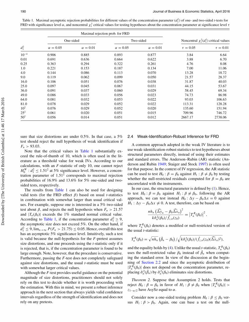
Table 1. Maximal asymptotic rejection probabilities for different values of the concentration parameter (d21 ) of one- and two-sided t-tests for

FRD with significance level α, and noncentral χ 21 critical values for testing hypotheses about the concentration parameter at significance level τ

Maximal rejection prob. for FRD

One-sided Two-sided Noncentral χ 21 (d2

1 ) critical values

d21 α = 0.05 α = 0.01 α = 0.05 α = 0.01 τ = 0.05 τ = 0.01

10−4 0.906 0.885 0.893 0.877 3.84 6.640.01 0.691 0.636 0.664 0.622 3.88 6.700.25 0.363 0.294 0.322 0.261 4.76 8.081.0 0.221 0.153 0.187 0.134 7.00 11.064.0 0.144 0.086 0.113 0.070 13.28 18.729.0 0.119 0.062 0.099 0.050 21.57 28.3716.0 0.106 0.051 0.076 0.038 31.87 40.0325.0 0.097 0.045 0.067 0.031 44.15 53.6736.0 0.091 0.037 0.060 0.029 58.45 69.3449.0 0.086 0.033 0.056 0.023 74.73 86.9864.0 0.081 0.032 0.053 0.022 93.03 106.6381.0 0.078 0.029 0.052 0.022 113.31 128.28102 0.076 0.029 0.052 0.020 135.60 151.94252 0.061 0.020 0.051 0.015 709.96 746.72502 0.056 0.014 0.051 0.012 2667.17 2738.06

sure that size distortions are under 0.5%. In that case, a 5%test should reject the null hypothesis of weak identification ifFn > 93.03.

Note that the critical values in Table 1 substantially ex-ceed the rule-of-thumb of 10, which is often used in the lit-erature as a threshold value for weak IVs. According to ourcalculations, with an F-statistic of only 10, one cannot rejectHW

0 : d21 ≤ 1.512 at 5% significance level. However, a concen-

tration parameter of 1.512 corresponds to maximal rejectionprobabilities of 16.9% and 13.6% for 5% one-sided and two-sided tests, respectively.

The results from Table 1 can also be used for designingvalid tests (for the FRD effect β) based on usual t-statisticsin combination with somewhat larger than usual critical val-ues. For example, suppose one is interested in a 5% two-sidedtest about β, and rejects the null hypothesis when Fn > 21.57and |Tn(β0)| exceeds the 1% standard normal critical value.According to Table 1, if the concentration parameter d2

1 ≥ 9,the asymptotic size does not exceed 5%. On the other hand, ifd2

1 ≤ 9, limn→∞ P (Fn > 21.75) ≤ 0.05. Hence, overall this testhas an asymptotic 5% significance level. Intuitively, such a testis valid because the null-hypothesis for the F-pretest assumessize distortions, and one proceeds using the t-statistic only if itis rejected, that is, if the concentration parameter is found to belarge enough. Note, however, that the procedure is conservative.Furthermore, passing the F-test does not completely safeguardagainst size distortions, and the usual t-statistic must be usedwith somewhat larger critical values.

Although the F-test provides useful guidance on the potentialmagnitude of size distortions, practitioners should not solelyrely on this test to decide whether it is worth proceeding withthe estimation. With this in mind, we present a robust inferenceapproach in the next section that always yields valid confidenceintervals regardless of the strength of identification and does notrely on any pretests.

2.4 Weak-Identification-Robust Inference for FRD

A common approach adopted in the weak IV literature is touse weak-identification-robust statistics to test hypotheses aboutstructural parameters directly, instead of using their estimatesand standard errors. The Anderson–Rubin (AR) statistic (An-derson and Rubin 1949; Staiger and Stock 1997) is often usedfor that purpose. In the context of IV regression, the AR statisticcan be used to test H0 : β = β0 against H1 : β �= β0 by testingwhether the null-restricted residuals computed for β = β0 areuncorrelated with the instruments.

In our case, the structural parameter is defined by (1). Hence,to test H0 : β = β0 against H1 : β �= β0, following the ARapproach, we can test instead H0 : �y − β0�x = 0 againstH1 : �y − β0�x �= 0. A test, therefore, can be based on

nhn

(�yn − β0�xn

)2

kσ 2n (β0)/fz,n(z0)

= ∣∣T Rn (β0)

∣∣2 ,

where T Rn (β0) denotes a modified or null-restricted version of

the usual t-statistic:

T Rn (β0) =

√nhn

(βn − β0

)/

√kσ 2

n (β0)/(fz,n(z0)(�xn)2),

and the equality holds by (4). Unlike the usual t-statistic, T Rn (β0)

uses the null-restricted value β0 instead of βn when comput-ing the standard error. In view of the discussion at the begin-ning of Section 2.2 and since the asymptotic distribution of|T R

n (β0)| does not depend on the concentration parameter, re-placing σ 2

n (βn) by σ 2n (β0) eliminates size distortions.

Theorem 2. Suppose that Assumption 2 holds. Tests thatreject H0 : β = β0 in favor of H1 : β �= β0 when |T R

n (β0)| >

z1−α/2 have AsySz equal to α.

Consider now a one-sided testing problem H0 : β ≤ β0 ver-sus H1 : β > β0. Again, one can base a test on the null-

Dow

nloa

ded

by [

The

Uni

vers

ity o

f B

ritis

h C

olum

bia]

at 1

1:46

17

Mar

ch 2

016

Feir, Lemieux, and Marmer: Weak Identification in Fuzzy Regression Discontinuity Designs 191

restricted statistic. In this case under H0 when β = β0, wehave T R

n (β) = (�Yn − β�Xn) × sign(�Xn ± dn,1

)/σ (β) +

op(1). When identification is strong or semistrong, dn,1 → ∞,and the sign term is constant with probability one. Since the firstterm is asymptotically N (0, 1), T R

n (β) is also asymptoticallyN (0, 1), and one could use standard normal critical values. Onthe other hand, when identification is weak and the concentra-tion parameter is small, the sign term is random, and therefore,the null asymptotic distribution of the product differs from stan-dard normal. To obtain an asymptotically uniformly valid test,one can use data-dependent critical values that automaticallyadjust to the strength of identification. Such critical values canbe generated using the approach of Moreira (2001, 2003) byconditioning on a statistic that is (i) asymptotically independentof �Yn − β�Xn, and (ii) summarizes the information on thestrength of identification (see also Andrews, Moreira, and Stock2006; Mills, Moreira, and Vilela 2014).

Define Sn = (�Yn − β�Xn)/σ (β) and Q = �Xn/σx −(σxy − βσ 2

x )Sn/(σxσ (β)), so that, when β = β0, T Rn (β) = Sn ×

sign[Qn ± dn,1 + (σxy − βσ 2x )Sn/(σxσ (β))] + op(1).

When identification is weak, Sn and Qn are asymptoticallyindependent by construction, while Sn →d N (0, 1). Therefore,one can construct data-dependent critical values as follows.First, compute

Qn(β0) =√

nhn�xn√kσ 2

x,n/fz,n(z0)− σxy,n − β0σ

2x,n

σx,nσn(β0)

×⎛⎝√

nhn

(�yn − β0�xn

)√kσ 2

n (β0)/fz,n(z0)

⎞⎠ .

Second, simulate M-independent N (0, 1) random variables{S1, . . . ,SM} for some large M. Third, for m = 1, . . . M com-pute

T Rn,m(β0, Qn(β0)) = Sm × sign

(Qn(β0) + σxy,n − β0σ

2x,n

σx,nσn(β0)Sm

).

Let cvn,1−α(β0, Qn(β0)) denote the (1 − α)th quantile of thesample distribution of {T R

n,m(β0, Qn(β0)) : m = 1, . . . , M}. Toobtain an asymptotically uniformly valid one-sided test, one canuse cvn,1−α(β0, Qn(β0)) as the critical value.

Theorem 3. Suppose that Assumption 2 holds. Tests thatreject H0 : β ≤ β0 in favor of H1 : β > β0 when T R

n (β0) >

cvn,1−α(β0, Qn(β0)) have AsySz equal to α.

Weak-identification-robust confidence sets for β can be con-structed by inversion of the robust tests. For example, a confi-dence set for β with asymptotic coverage probability 1 − α canbe constructed by collecting all values β0 that cannot be rejectedby the two-sided robust test:

CS1−α,n = {β0 ∈ R :

∣∣T Rn (β0)

∣∣ ≤ z1−α/2}. (9)

This confidence set can be easily computed analytically by solv-ing for values of β0 that satisfy the inequality

(βn − β0)2σ 2x,nFn − z2

1−α/2(σ 2y,n + β2

0 σ 2x,n − 2σxy,nβ0) ≤ 0, (10)

where Fn is defined in (8).Depending on the coefficients of the second-order polynomial

(in β0) in Equation (10), CS1−α,n can take one of the following

forms: (i) an interval, (ii) a union of two disconnected half-lines(−∞, a1] ∪ [a2,∞), where a1 < a2, or (iii) the entire real line.One will see cases (ii) or (iii) if the coefficient on β2

0 in (10) isnegative, which occurs when

Fn − z21−α/2 < 0. (11)

Thus, in practice one will see nonstandard confidence sets if thenull hypothesis �x = 0 cannot be rejected using the F-statisticand central χ2

1,1−α critical values. Case (iii) arises when thediscriminant of the quadratic polynomial in (10) is negative,which occurs if

Fnσ2n (βn) − z2

1−α/2

(σ 2

y,n − σ 2xy,n/σ

2x,n

)< 0. (12)

Positive definiteness of the variance-covariance matrix com-posed of σ 2

x,n, σ 2y,n, and σxy,n implies that (11) holds whenever

(12) holds. Thus, negative discriminants implied by (12) areinconsistent with Fn > z2

1−α/2 or positive coefficients on β20 in

(10). This in turn implies that CS1−α,n cannot be empty.When identification is strong or semistrong, the concentra-

tion parameter and, therefore, Fn diverge to infinity. In suchcases, both the discriminant and the coefficient on β2

0 tend tobe positive, and consequently, CS1−α,n will be an interval withprobability approaching one.

Furthermore, one can show that when identification is strongand under local alternatives of the form β = β0 + μ/(nhn)1/2,tests based on Tn(β0) and T R

n (β0) have the same asymptoticpower. Thus, in practice there is no loss of asymptotic powerfrom adopting the robust inference approach if identification isstrong.

3. TESTING FOR CONSTANCY OF THE RD EFFECTACROSS COVARIATES

In this section, we develop a test of constancy of the RD effectacross covariates, which is robust to weak identification issues.Such a test can be useful in practice when the econometricianwants to argue that the treatment effect is different for differentpopulation subgroups. For example, in Section 4, we use this testto argue that the effect of class sizes on educational achievementsis different for secular and religious schools, and therefore itmight be optimal to implement different rules concerning classsizes in those two categories of schools. The problem is relatedto the classical analysis of variance (ANOVA) hypothesis ofhomogenous populations (see, e.g., Casella and Berger 2002,chap. 11).

Similarly to Otsu, Xu, and Matsushita (2015), we consider theRD effect conditional on some covariate wi . (See also Frolich2007.) Let W denote the support of the distribution of wi . Next,for w ∈ W we define y+(w) using the conditional expectationgiven zi and wi = w: y+(w) = limz↓z0 E (yi |zi = z,wi = w) .

Let y−(w), x+(w), and x−(w) be defined similarly. The condi-tional RD effect given wi = w is defined as β(w) = (y+(w) −y−(w))/(x+(w) − x−(w)). Similarly to the case without covari-ates, under an appropriate set of assumptions, β(w) captures the(local) ATE at z0 conditional on wi = w. We are interested intesting the null hypothesis of constancy of the RD effect

H0 : β(w) = β for some β ∈ R and all w ∈ W, (13)

against a general alternative H1 : β(w) �= β(v) for some v,w ∈W. When identification is strong, the econometrician can esti-

Dow

nloa

ded

by [

The

Uni

vers

ity o

f B

ritis

h C

olum

bia]

at 1

1:46

17

Mar

ch 2

016

192 Journal of Business & Economic Statistics, April 2016

mate the conditional RD effect function consistently and thenuse it for testing of H0. (Such a test can be constructed similarlyto the ANOVA F-test as in Casella and Berger (2002, chap. 11)and is discussed in the supplement.) However, this approachcan be unreliable if identification is weak. We therefore take analternative approach.

Suppose thatW = {w1, . . . , wJ }, that is, the covariate is cate-gorical and divides the population into J groups. The assumptionof a categorical covariate is plausible in many practical applica-tions where the econometrician may be interested in the effectof gender, school type, etc. However, even when the covariate iscontinuous, in a nonparametric framework it might be sensibleto categorize it to have sufficient power (as is often done inpractice). For j = 1, . . . , J , let y+

n (wj ), y−n (wj ), x+

n (wj ), andx−

j,n(wj ) denote the local linear estimators of the correspondingpopulation terms computed using only the observations withwi = wj . Let nj be the number of such observations. Defineσ 2

y (wj ), σ 2x (wj ), and σxy(wj ) as the conditional versions of the

corresponding population terms, and let σ 2y,n(wj ), σ 2

x,n(wj ), andσxy,n(wj ) denote the corresponding estimators.

Suppose that Assumption 2 holds for each of the J cate-gories, and none of the categories is redundant asymptotically:njhnj

/(nhn) → pj > 0 for j = 1, . . . , J , where n = ∑Jj=1 nj .

If H0 is true and the FRD effect is independent of w, onecan construct a robust confidence set for the common effect:CSJ

1−α,n = {β0 ∈ R : Gn(β0) ≤ χ2

J,1−α

}, where

Gn(β0) =J∑

j=1

njhnj

(βn(wj ) − β0

)2

kσ 2n (β0, wj )/(fz,n(z0|wj )(�xn(wj ))2)

,

βn(wj ) = �yn(wj )/�xn(wj ), �xn(wj ) = x+n (wj ) − x−

n (wj );σ 2

n (β0, wj ) is defined similarly to σ 2

n (β0) in (3) usingthe estimators conditional on wi = wj ; and fz,n(z0|wj ) =(njhnj

)−1∑ni=1 K((zi − z0)/hnj

)1{wi = wj } is the estimatorfor fz(z0|wj ), which denotes the conditional density of zi atz0 conditional on wi = wj .

Under H0 : β(w) = β for some β ∈ R, CSJ1−α,n is an asymp-

totically valid confidence set since Gn(β) →d χ2J under weak or

strong identification. We consider the following size α asymp-totic test: Reject H0 if CSJ

1−α,n is empty. The test is asymp-totically valid because under H0, P (CSJ

1−α,n = ∅) ≤ P (β /∈CSJ

1−α,n) = P (Gn(β) > χ2J,1−α) → α, which again holds under

weak or strong identification. Under the alternative, there is nocommon value β that will provide a proper recentering for allJ categories, and therefore, one can expect deviations from theasymptotic χ2

J distribution.We show below that the test is consistent if there is strong (or

semistrong) identification for at least two values wj1 and wj2

that satisfy β(wj1 ) �= β(wj2 ). Let d2n,1(wj ) = njhnj

|x+(wj ) −x−(wj )|2fz(z0|wj )/(kσ 2

x (wj )) be the conditional version of theconcentration parameter.

Theorem 4. Suppose that njhnj/(nhn) → pj > 0 and As-

sumption 2 holds for each j = 1, . . . , J .

a. Tests that reject H0 of constancy in (13) when CSJ1−α,n =

∅ have AsySz less or equal to α.

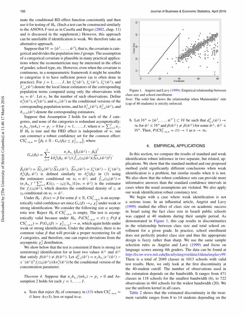
Figure 1. Angrist and Lavy (1999): Empirical relationship betweenclass size and school enrollment.Note: The solid line shows the relationship when Maimonides’ rule(cap of 40 students) is strictly enforced.

b. Let W∗ = {w1, . . . , wJ ∗ } ⊂ W be such that d2n,1(wj ) →

∞ for wj ∈ W∗ and β(wj1 ) �= β(wj2 ) for some wj1 , wj2 ∈W∗. Then, P (CSJ

1−α,n = ∅) → 1 as n → ∞.

4. EMPIRICAL APPLICATIONS

In this section, we compare the results of standard and weakidentification robust inference in two separate, but related, ap-plications. We show that the standard method and our proposedmethod yield significantly different conclusions when weakidentification is a problem, but similar results when it is not.We also show that the robust confidence sets can provide moreinformative answers than the standard confidence intervals incases when the usual assumptions are violated. We also applyour weak identification robust constancy test.

We begin with a case where weak identification is nota serious issue. In an influential article, Angrist and Lavy(1999) studied the effect of class size on academic successin Israel using the fact class size in Israeli public schoolswas capped at 40 students during their sample period. Asdemonstrated in Figure 1, this cap results in discontinuitiesin the relationship between class size and total school en-rollment for a given grade. In practice, school enrollmentdoes not perfectly predict class size and thus the appropriatedesign is fuzzy rather than sharp. We use the same sampleselection rules as Angrist and Lavy (1999) and focus onlanguage scores among 4th graders. The data can be found athttp://econ-www.mit.edu/faculty/angrist/data1/data/anglavy99.There is a total of 2049 classes in 1013 schools with validtest results. Here, we only look at the first discontinuity atthe 40-student cutoff. The number of observations used inthe estimation depends on the bandwidth. It ranges from 471classes in 118 schools for the smallest bandwidth (6), to 722observations in 484 schools for the widest bandwidth (20). Weuse the uniform kernel in all cases.

Table 2 shows that the estimated discontinuity in the treat-ment variable ranges from 8 to 14 students depending on the

Dow

nloa

ded

by [

The

Uni

vers

ity o

f B

ritis

h C

olum

bia]

at 1

1:46

17

Mar

ch 2

016

Feir, Lemieux, and Marmer: Weak Identification in Fuzzy Regression Discontinuity Designs 193

Table 2. Angrist and Lavy (1999): Estimated discontinuity in the treatment variable for the first cutoff and their standard errors, estimatedeffect of class size on class average verbal score, and standard and robust 95% confidence sets (CSs) for the class size effect for different values

of the bandwidth

Bandwidth Discont. Std. errors F-stat Effect Standard CS Robust CS

6 −8.40 1.60 27.5 −0.07 [−0.145, 0.007] [−0.170, −0.000]8 −9.90 1.26 61.9 −0.07 [−0.129, −0.015] [−0.138, −0.019]10 −10.83 1.03 110.2 −0.06 [−0.103,-0.015] [−0.103,-0.015]12 −12.00 0.92 172.0 −0.02 [−0.056, 0.011] [−0.058, 0.010]14 −12.62 0.78 258.8 −0.03 [−0.061, 0.000] [−0.062, −0.000]16 −13.21 0.69 370.1 −0.02 [−0.048, 0.008] [−0.049, 0.007]18 −13.87 0.61 525.8 −0.02 [−0.046, 0.003] [−0.047, 0.003]20 −14.35 0.56 667.7 −0.02 [−0.042, 0.005] [−0.043, 0.004]

NOTES: Silverman’s normal rule-of-thumb bandwidth is 7.84 and the optimal bandwidth suggested by Imbens and Kalyanaraman (2012) is 7.90. The scores are given in terms of standarddeviations from the mean.

bandwidth chosen. The table also shows that, as expected, theF-statistic becomes smaller as the bandwidth gets smaller. Sil-verman’s normal rule-of-thumb and the optimal bandwidth pro-cedure of Imbens and Kalyanaraman (2012) both suggest abandwidth value of approximately 8, which corresponds to arelatively large value of the F-statistic (approximately 62). Ap-plying the standards of Table 1, we then conclude that weakidentification is not a serious concern in this application. Usingthe 5% noncentral χ2 critical value, we reject the null hypothesisthat the concentration parameter is below 36, and therefore, themaximal size distortions of the 5% two-sided tests are expectedto be under 1%. Note that even at the smallest bandwidth, theF-statistic is relatively large. This is consistent with Figure 2that shows that the 95% standard and robust confidence sets forthe class size effect are very similar. The figure shows that thetwo sets of confidence intervals are essentially indistinguish-able for larger bandwidths, and only differ slightly for smallerbandwidths.

In this application, we also compare the results of the stan-dard constancy test of the treatment effect across subgroups tothe results of our robust constancy test. The first set of resultsreported in Section 5 of the online supplement compares the

Figure 2. Angrist and Lavy (1999): 95% confidence intervals forthe effect of class size on verbal test scores for different values of thebandwidth.Note: This figure is for the enrollment cutoff of 40. The bandwidthaccording to Silverman’s normal rule-of-thumb is 7.94. The optimalbandwidth selected according to Imbens and Kalyanaraman (2012) is7.90. The scores are given in terms of standard deviations from themean.

treatment effect for secular and religious schools. The null hy-pothesis (the treatment effect is the same across subgroups) cannever be rejected using a standard test. By contrast, the robustconstancy test rejects the null hypothesis for the largest valuesof the bandwidth (18 and 20). We reach similar conclusionswhen comparing the treatment effect for schools with aboveand below median proportions of disadvantaged students. Thenull hypothesis is rejected by the robust test under the largestbandwidth (20). This suggests that our proposed test may havegreater power against alternatives than the standard test in somecontexts.

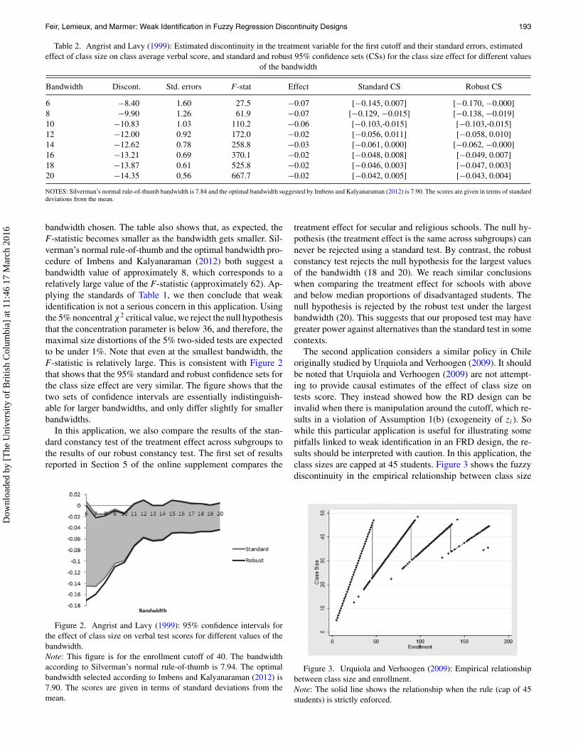
The second application considers a similar policy in Chileoriginally studied by Urquiola and Verhoogen (2009). It shouldbe noted that Urquiola and Verhoogen (2009) are not attempt-ing to provide causal estimates of the effect of class size ontests score. They instead showed how the RD design can beinvalid when there is manipulation around the cutoff, which re-sults in a violation of Assumption 1(b) (exogeneity of zi). Sowhile this particular application is useful for illustrating somepitfalls linked to weak identification in an FRD design, the re-sults should be interpreted with caution. In this application, theclass sizes are capped at 45 students. Figure 3 shows the fuzzydiscontinuity in the empirical relationship between class size

Figure 3. Urquiola and Verhoogen (2009): Empirical relationshipbetween class size and enrollment.Note: The solid line shows the relationship when the rule (cap of 45students) is strictly enforced.

Dow

nloa

ded

by [

The

Uni

vers

ity o

f B

ritis

h C

olum

bia]

at 1

1:46

17

Mar

ch 2

016

194 Journal of Business & Economic Statistics, April 2016

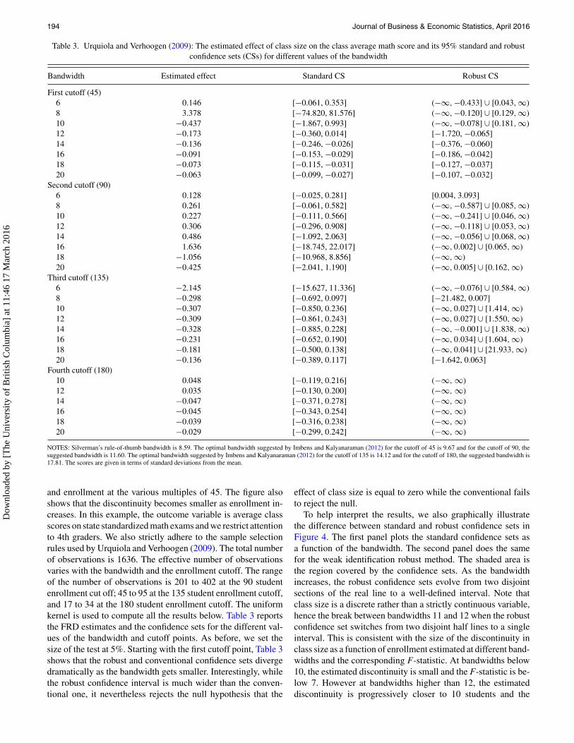
Table 3. Urquiola and Verhoogen (2009): The estimated effect of class size on the class average math score and its 95% standard and robustconfidence sets (CSs) for different values of the bandwidth

Bandwidth Estimated effect Standard CS Robust CS

First cutoff (45)6 0.146 [−0.061, 0.353] (−∞, −0.433] ∪ [0.043, ∞)8 3.378 [−74.820, 81.576] (−∞, −0.120] ∪ [0.129, ∞)10 −0.437 [−1.867, 0.993] (−∞, −0.078] ∪ [0.181, ∞)12 −0.173 [−0.360, 0.014] [−1.720, −0.065]14 −0.136 [−0.246, −0.026] [−0.376, −0.060]16 −0.091 [−0.153, −0.029] [−0.186, −0.042]18 −0.073 [−0.115, −0.031] [−0.127, −0.037]20 −0.063 [−0.099, −0.027] [−0.107, −0.032]

Second cutoff (90)6 0.128 [−0.025, 0.281] [0.004, 3.093]8 0.261 [−0.061, 0.582] (−∞, −0.587] ∪ [0.085, ∞)10 0.227 [−0.111, 0.566] (−∞, −0.241] ∪ [0.046, ∞)12 0.306 [−0.296, 0.908] (−∞, −0.118] ∪ [0.053, ∞)14 0.486 [−1.092, 2.063] (−∞, −0.056] ∪ [0.068, ∞)16 1.636 [−18.745, 22.017] (−∞, 0.002] ∪ [0.065, ∞)18 −1.056 [−10.968, 8.856] (−∞, ∞)20 −0.425 [−2.041, 1.190] (−∞, 0.005] ∪ [0.162, ∞)

Third cutoff (135)6 −2.145 [−15.627, 11.336] (−∞, −0.076] ∪ [0.584, ∞)8 −0.298 [−0.692, 0.097] [−21.482, 0.007]10 −0.307 [−0.850, 0.236] (−∞, 0.027] ∪ [1.414, ∞)12 −0.309 [−0.861, 0.243] (−∞, 0.027] ∪ [1.550, ∞)14 −0.328 [−0.885, 0.228] (−∞, −0.001] ∪ [1.838, ∞)16 −0.231 [−0.652, 0.190] (−∞, 0.034] ∪ [1.604, ∞)18 −0.181 [−0.500, 0.138] (−∞, 0.041] ∪ [21.933, ∞)20 −0.136 [−0.389, 0.117] [−1.642, 0.063]

Fourth cutoff (180)10 0.048 [−0.119, 0.216] (−∞, ∞)12 0.035 [−0.130, 0.200] (−∞, ∞)14 −0.047 [−0.371, 0.278] (−∞, ∞)16 −0.045 [−0.343, 0.254] (−∞, ∞)18 −0.039 [−0.316, 0.238] (−∞, ∞)20 −0.029 [−0.299, 0.242] (−∞, ∞)

NOTES: Silverman’s rule-of-thumb bandwidth is 8.59. The optimal bandwidth suggested by Imbens and Kalyanaraman (2012) for the cutoff of 45 is 9.67 and for the cutoff of 90, thesuggested bandwidth is 11.60. The optimal bandwidth suggested by Imbens and Kalyanaraman (2012) for the cutoff of 135 is 14.12 and for the cutoff of 180, the suggested bandwidth is17.81. The scores are given in terms of standard deviations from the mean.

and enrollment at the various multiples of 45. The figure alsoshows that the discontinuity becomes smaller as enrollment in-creases. In this example, the outcome variable is average classscores on state standardized math exams and we restrict attentionto 4th graders. We also strictly adhere to the sample selectionrules used by Urquiola and Verhoogen (2009). The total numberof observations is 1636. The effective number of observationsvaries with the bandwidth and the enrollment cutoff. The rangeof the number of observations is 201 to 402 at the 90 studentenrollment cut off; 45 to 95 at the 135 student enrollment cutoff,and 17 to 34 at the 180 student enrollment cutoff. The uniformkernel is used to compute all the results below. Table 3 reportsthe FRD estimates and the confidence sets for the different val-ues of the bandwidth and cutoff points. As before, we set thesize of the test at 5%. Starting with the first cutoff point, Table 3shows that the robust and conventional confidence sets divergedramatically as the bandwidth gets smaller. Interestingly, whilethe robust confidence interval is much wider than the conven-tional one, it nevertheless rejects the null hypothesis that the

effect of class size is equal to zero while the conventional failsto reject the null.

To help interpret the results, we also graphically illustratethe difference between standard and robust confidence sets inFigure 4. The first panel plots the standard confidence sets asa function of the bandwidth. The second panel does the samefor the weak identification robust method. The shaded area isthe region covered by the confidence sets. As the bandwidthincreases, the robust confidence sets evolve from two disjointsections of the real line to a well-defined interval. Note thatclass size is a discrete rather than a strictly continuous variable,hence the break between bandwidths 11 and 12 when the robustconfidence set switches from two disjoint half lines to a singleinterval. This is consistent with the size of the discontinuity inclass size as a function of enrollment estimated at different band-widths and the corresponding F-statistic. At bandwidths below10, the estimated discontinuity is small and the F-statistic is be-low 7. However at bandwidths higher than 12, the estimateddiscontinuity is progressively closer to 10 students and the

Dow

nloa

ded

by [

The

Uni

vers

ity o

f B

ritis

h C

olum

bia]

at 1

1:46

17

Mar

ch 2

016

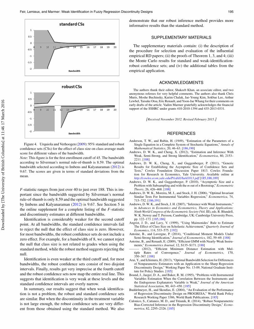
Feir, Lemieux, and Marmer: Weak Identification in Fuzzy Regression Discontinuity Designs 195

Figure 4. Urquiola and Verhoogen (2009): 95% standard and robustconfidence sets (CSs) for the effect of class size on class average mathscore for different values of the bandwidth.Note: This figure is for the first enrollment cutoff of 45. The bandwidthaccording to Silverman’s normal rule-of-thumb is 8.59. The optimalbandwidth selected according to Imbens and Kalyanaraman (2012) is9.67. The scores are given in terms of standard deviations from themean.

F-statistic ranges from just over 40 to just over 188. This is im-portant since the bandwidth suggested by Silverman’s normalrule-of-thumb is only 8.59 and the optimal bandwidth suggestedby Imbens and Kalyanaraman (2012) is 9.67. See Section 5 inthe online supplement for a complete listing of the F-statisticand discontinuity estimates at different bandwidths.

Identification is considerably weaker for the second cutoffpoint. At all bandwidths, the standard confidence intervals failto reject the null that the effect of class size is zero. However,for most bandwidths, the robust confidence sets do not include azero effect. For example, for a bandwidth of 8, we cannot rejectthe null that class size is not related to grades when using thestandard method, while the robust method suggests rejecting thenull.

Identification is even weaker at the third cutoff and, for mostbandwidths, the robust confidence sets consist of two disjointintervals. Finally, results get very imprecise at the fourth cutoffand the robust confidence sets now map the entire real line. Thissuggests that identification is very weak at these levels and thestandard confidence intervals are overly narrow.

In summary, our results suggest that when weak identifica-tion is not a problem, the robust and standard confidence setsare similar. But when the discontinuity in the treatment variableis not large enough, the robust confidence sets are very differ-ent from those obtained using the standard method. We also

demonstrate that our robust inference method provides moreinformative results than the standard method.

SUPPLEMENTARY MATERIALS

The supplementary materials contain: (i) the description ofthe procedure for selection and evaluation of the influentialempirical RD papers; (ii) the proofs of Theorem 1, 3, and 4; (iii)the Monte Carlo results for standard and weak-identification-robust confidence sets; and (iv) the additional tables from theempirical application.

ACKNOWLEDGMENTS

The authors thank their editor, Shakeeb Khan, an associate editor, and twoanonymous referees for very helpful comments. The authors also thank ChrisMuris, Moshe Buchinsky, Karim Chalak, Jae-Young Kim, Sokbae Lee, ArthurLewbel, Taisuke Otsu, Eric Renault, and Yoon-Jae Whang for their comments onearly drafts of the article. Vadim Marmer gratefully acknowledges the financialsupport of the SSHRC under grants 410-2010-1394 and 435-2013-0331.

[Received November 2012. Revised February 2015.]

REFERENCES

Anderson, T. W., and Rubin, H. (1949), “Estimation of the Parameters of aSingle Equation in a Complete System of Stochastic Equations,” Annals ofMathematical Statistics, 20, 46–63. [186,190]

Andrews, D. W. K., and Cheng, X. (2012), “Estimation and Inference WithWeak, Semi-Strong, and Strong Identification,” Econometrica, 80, 2153–2211. [188]

Andrews, D. W. K., Cheng, X., and Guggenberger, P. (2011), “GenericResults for Establishing the Asymptotic Size of Confidence Sets andTests,” Cowles Foundation Discussion Paper 1813. Cowles Founda-tion for Research in Economics, Yale University. Available online athttp://cowles.econ.yale.edu/P/cd/d18a/d1813.pdf [185,188,189]

Andrews, D. W. K., and Guggenberger, P. (2010), “Asymptotic Size and aProblem with Subsampling and with the m out of n Bootstrap,” EconometricTheory, 26, 426–468. [188]

Andrews, D. W. K., Moreira, M. J., and Stock, J. H. (2006), “Optimal InvariantSimilar Tests For Instrumental Variables Regression,” Econometrica, 74,715–752. [186,191]

Andrews, D. W. K., and Stock, J. H. (2007), “Inference with Weak Instruments,”in Advances in Economics and Econometrics, Theory and Applications:Ninth World Congress of the Econometric Society (Vol. III), eds. R. Blundell,W. K. Newey and T. Persson, Cambridge, UK: Cambridge University Press,pp. 122–173. [185,186]

Angrist, J. D., and Lavy, V. (1999), “Using Maimonides’ Rule to EstimateThe Effect of Class Size on Scholastic Achievement,” Quarterly Journal ofEconomics, 114, 533–575. [192]

Antoine, B., and Lavergne, P. (2014), “Conditional Moment Models UnderSemi-Strong Identification,” Journal of Econometrics, 182, 59–69. [188]

Antoine, B., and Renault, E. (2009), “Efficient GMM with Nearly-Weak Instru-ments,” Econometrics Journal, 12, S135–S171. [188]

——— (2012), “Efficient Minimum Distance Estimation with Mul-tiple Rates of Convergence,” Journal of Econometrics, 170,350–367. [188]

Arai, Y., and Ichimura, H. (2013), “Optimal Bandwidth Selection for Differencesof Nonparametric Estimators with an Application to the Sharp RegressionDiscontinuity Design,” Working Paper No. 13-09, National Graduate Insti-tute for Policy Studies. [185]

Bound, J., Jaeger, D. A., and Baker, R. M. (1995), “Problems with InstrumentalVariables Estimation When the Correlation Between the Instruments andthe Endogenous Explanatory Variable is Weak,” Journal of the AmericanStatistical Association, 90, 443–450. [185]

Buddelmeyer, H., and Skoufias, E. (2004), “An Evaluation of the Performanceof Regression Discontinuity Design on PROGRESA,” World Bank PolicyResearch Working Paper 3386, World Bank Publications. [185]

Calonico, S., Cattaneo, M. D., and Titiunik, R. (2014), “Robust NonparametricBias-Corrected Inference in the Regression Discontinuity Design,” Econo-metrica, 82, 2295–2326. [185]

Dow

nloa

ded

by [

The

Uni

vers

ity o

f B

ritis

h C

olum

bia]

at 1

1:46

17

Mar

ch 2

016

196 Journal of Business & Economic Statistics, April 2016

Caner, M. (2009), “Testing, Estimation in GMM and CUE with Nearly-WeakIdentification,” Econometric Reviews, 29, 330–363. [188]

Casella, G., and Berger, R. L. (2002), Statistical Inference (2nd ed.), PacificGrove, CA: Duxbury Press. [191]

Davidson, J. (1994), Stochastic Limit Theory, New York: Oxford UniversityPress. [187]

Dong, Y., and Lewbel, A. (2010), “Regression Discontinuity Marginal ThresholdTreatment Effects,” Working Paper No. 759, Boston College. [185]

Dufour, J.-M. (1997), “Some Impossibility Theorems in Econometrics withApplications to Structural and Dynamic Models,” Econometrica, 65, 1365–1387. [186]

Fe, E. (2012), “Efficient Estimation in Regression Discontinuity Designs viaAsymmetric Kernels,” MPRA Working Paper No. 38164, Munich PersonalRePEc Archive. Available at http://mpra.ub.uni-muenchen.de/38164/. [185]

Frolich, M. (2007), “Regression Discontinuity Design with Covariates,” Work-ing Paper 2007-32, University of St. Gallen. [185,191]

Frolich, M., and Melly, B. (2008), “Quantile Treatment Effects in the RegressionDiscontinuity Design,” IZA Discussion Paper 3638, Institute for the Studyof Labor. [185]

Hahn, J., and Kuersteiner, G. (2002), “Discontinuities of Weak InstrumentLimiting Distributions,” Economics Letters, 75, 325–331. [188]

Hahn, J., Todd, P., and Van der Klaauw, W. (1999), “Evaluating the Ef-fect of an Antidiscrimination Law Using a Regression-DiscontinuityDesign,” NBER Working Paper 7131, National Bureau of EconomicResearch. [185,187]

——— (2001), “Identification and Estimation of Treatment Effects with aRegression-Discontinuity Design,” Econometrica, 69, 201–209. [185,187]

Imbens, G. W., and Kalyanaraman, K. (2012), “Optimal Bandwidth Choice forthe Regression Discontinuity Estimator,” Review of Economic Studies, 79,933–959. [185,193,194,195]

Imbens, G. W., and Lemieux, T. (2008), “Regression Discontinuity Designs: AGuide to Practice,” Journal of Econometrics, 142, 615–635. [185,187]

Imbens, G. W., and Manski, C. F. (2004), “Confidence Intervals for PartiallyIdentified Parameters,” Econometrica, 72, 1845–1857. [188]

Kleibergen, F. (2002), “Pivotal Statistics For Testing Structural Parametersin Instrumental Variables Regression,” Econometrica, 70, 1781–1803.[186]

Lee, D. S., and Lemieux, T. (2010), “Regression Discontinuity De-signs in Economics,” Journal of Economic Literature, 48, 281–355.[185]

McCrary, J. (2008), “Manipulation of the Running Variable in the RegressionDiscontinuity Design: A Density Test,” Journal of Econometrics, 142, 698–714. [185]

Mikusheva, A. (2007), “Uniform Inference in Autoregressive Models,” Econo-metrica, 75, 1411–1452. [188]

Mills, B., Moreira, M. J., and Vilela, L. P. (2014), “Tests Based on t-Statisticsfor IV Regression with Weak Instruments,” Journal of Econometrics, 182,351–363. [191]

Moreira, M. J. (2001), “Tests with Correct Size When Instruments Can Be Ar-bitrarily Weak,” unpublished manuscript, Department of Economics, Uni-versity of California, Berkeley. [186,191]

——— (2003), “A Conditional Likelihood Ratio Test For Structural Models,”Econometrica, 71, 1027–1048. [186,191]

Otsu, T., Xu, K.-L., and Matsushita, Y. (2015), “Empirical Likelihood for Re-gression Discontinuity Design,” Journal of Econometrics, 186, 94–112.[185,186,191]

Papay, J. P., Willett, J. B., and Murnane, R. J. (2011), “Extending the Regression-Discontinuity Approach to Multiple Assignment Variables,” Journal ofEconometrics, 161, 203–207. [185]

Porter, J. (2003), “Estimation in the Regression Discontinuity Model,” WorkingPaper, University of Wisconsin-Madison. [185]

Staiger, D., and Stock, J. H. (1997), “Instrumental Variables Regression WithWeak Instruments,” Econometrica, 65, 557–586. [185,188,190]

Stock, J. H., Wright, J. H., and Yogo, M. (2002), “A Survey of Weak Instrumentsand Weak Identification in Generalized Method of Moments,” Journal ofBusiness & Economic Statistics, 20. [185]

Stock, J. H., and Yogo, M. (2005), “Testing for Weak Instruments in Lin-ear IV Regression,” in Identification and Inference for Econometric Mod-els: Essays in Honor of Thomas Rothenberg, eds. D. W. K. Andrewsand J. H. Stock, New York: Cambridge University Press, pp. 80–108.[186,189]

Urquiola, M., and Verhoogen, E. (2009), “Class-Size Caps, Sorting, and theRegression-Discontinuity Design,” American Economic Review, 99, 179–215. [193,195]

Van der Klaauw, W. (2008), “Regression–Discontinuity Analysis: A Survey ofRecent Developments in Economics,” Labour, 22, 219–245. [185]

Zajonc, T. (2012), “Regression Discontinuity Design with Multiple Forc-ing Variables,” in Essays on Causal Inference for Public Policy, Chap-ter 2, Doctoral Dissertation, Harvard University, pp. 45–81. Available athttp://nrs.harvard.edu/urn-3:HUL.InstRepos:9368030 [185]

Dow

nloa

ded

by [

The

Uni

vers

ity o

f B

ritis

h C

olum

bia]

at 1

1:46

17

Mar

ch 2

016