
Stabilizing the Benjamin–Feir instability
43
J. Fluid Mech. (2005), vol. 539, pp. 229–271. c 2005 Cambridge University Press doi:10.1017/S002211200500563X Printed in the United Kingdom 229 Stabilizing the Benjamin–Feir instability By HARVEY SEGUR 1 , DIANE HENDERSON 2 , JOHN CARTER 3 , JOE HAMMACK 2 †, CONG-MING LI 1 , DANA PHEIFF 2 AND KATHERINE SOCHA 4 1 Department of Applied Mathematics, University of Colorado, Boulder, CO 80309-0526, USA 2 William G. Pritchard Fluid Mechanics Laboratory, Department of Mathematics, Penn State University, University Park, PA 16802, USA 3 Department of Mathematics, Seattle University, Seattle, WA 98122-4340, USA 4 Mathematics Department, Lyman Briggs School, Michigan State University, East Lansing, MI 48825-1107, USA (Received 19 February 2004 and in revised form 6 April 2005) The Benjamin–Feir instability is a modulational instability in which a uniform train of oscillatory waves of moderate amplitude loses energy to a small perturbation of other waves with nearly the same frequency and direction. The concept is well established in water waves, in plasmas and in optics. In each of these applications, the nonlinear Schr¨ odinger equation is also well established as an approximate model based on the same assumptions as required for the derivation of the Benjamin–Feir theory: a narrow-banded spectrum of waves of moderate amplitude, propagating primarily in one direction in a dispersive medium with little or no dissipation. In this paper, we show that for waves with narrow bandwidth and moderate amplitude, any amount of dissipation (of a certain type) stabilizes the instability. We arrive at this stability result first by proving it rigorously for a damped version of the nonlinear Schr¨ odinger equation, and then by confirming our theoretical predictions with laboratory experi- ments on waves of moderate amplitude in deep water. The Benjamin–Feir instability is often cited as the first step in a nonlinear process that spreads energy from an initially narrow bandwidth to a broader bandwidth. In this process, sidebands grow exponentially until nonlinear interactions eventually bound their growth. In the pres- ence of damping, this process might still occur, but our work identifies another possibi- lity: damping can stop the growth of perturbations before nonlinear interactions become important. In this case, if the perturbations are small enough initially, then they never grow large enough for nonlinear interactions to become important. 1. Introduction In a landmark paper, Benjamin & Feir (1967) showed that a uniform train of plane waves of moderate amplitude in deep water without dissipation is unstable to a small perturbation of other waves travelling in the same direction with nearly the same frequency. The instability is a finite-amplitude effect, in the sense that the unperturbed wavetrain (which we call the ‘carrier wave’) must have finite amplitude, and the growth rate of the instability is proportional to the square of that amplitude, at least for small amplitudes. Corroborating theoretical results were obtained about the same † Professor Hammack died during the publication process of this paper.
Transcript of Stabilizing the Benjamin–Feir instability
J. Fluid Mech. (2005), vol. 539, pp. 229–271. c© 2005 Cambridge University Press
doi:10.1017/S002211200500563X Printed in the United Kingdom
229
Stabilizing the Benjamin–Feir instability
By HARVEY SEGUR1, DIANE HENDERSON2,JOHN CARTER3, JOE HAMMACK2†, CONG-MING LI1,
DANA PHEIFF2 AND KATHERINE SOCHA4
1Department of Applied Mathematics, University of Colorado, Boulder, CO 80309-0526, USA2William G. Pritchard Fluid Mechanics Laboratory, Department of Mathematics, Penn State University,
University Park, PA 16802, USA3Department of Mathematics, Seattle University, Seattle, WA 98122-4340, USA
4Mathematics Department, Lyman Briggs School, Michigan State University, East Lansing,MI 48825-1107, USA
(Received 19 February 2004 and in revised form 6 April 2005)
The Benjamin–Feir instability is a modulational instability in which a uniform train ofoscillatory waves of moderate amplitude loses energy to a small perturbation of otherwaves with nearly the same frequency and direction. The concept is well establishedin water waves, in plasmas and in optics. In each of these applications, the nonlinearSchrodinger equation is also well established as an approximate model based onthe same assumptions as required for the derivation of the Benjamin–Feir theory: anarrow-banded spectrum of waves of moderate amplitude, propagating primarily inone direction in a dispersive medium with little or no dissipation. In this paper, weshow that for waves with narrow bandwidth and moderate amplitude, any amountof dissipation (of a certain type) stabilizes the instability. We arrive at this stabilityresult first by proving it rigorously for a damped version of the nonlinear Schrodingerequation, and then by confirming our theoretical predictions with laboratory experi-ments on waves of moderate amplitude in deep water. The Benjamin–Feir instabilityis often cited as the first step in a nonlinear process that spreads energy from aninitially narrow bandwidth to a broader bandwidth. In this process, sidebands growexponentially until nonlinear interactions eventually bound their growth. In the pres-ence of damping, this process might still occur, but our work identifies another possibi-lity: damping can stop the growth of perturbations before nonlinear interactionsbecome important. In this case, if the perturbations are small enough initially, thenthey never grow large enough for nonlinear interactions to become important.
1. IntroductionIn a landmark paper, Benjamin & Feir (1967) showed that a uniform train of plane
waves of moderate amplitude in deep water without dissipation is unstable to a smallperturbation of other waves travelling in the same direction with nearly the samefrequency. The instability is a finite-amplitude effect, in the sense that the unperturbedwavetrain (which we call the ‘carrier wave’) must have finite amplitude, and the growthrate of the instability is proportional to the square of that amplitude, at least forsmall amplitudes. Corroborating theoretical results were obtained about the same
† Professor Hammack died during the publication process of this paper.
230 H. Segur and others
time by Lighthill (1965), Ostrovsky (1967), Whitham (1967), Benney & Newell (1967),and Zakharov (1967, 1968). We note particularly that Zakharov (1968) derived thenonlinear Schrodinger (NLS) equation,
i∂tψ + α∂2xψ + β∂2
yψ + γ |ψ |2ψ = 0, (1.1)
where α, β, γ are real-valued constants, to describe approximately the slow evolutionof the complex envelope of a nearly monochromatic train of plane waves of moderateamplitude in deep water. (Zakharov actually considered the one-dimensional versionof (1.1), with β = 0.) Equation (1.1) is more general than the work of Benjamin &Feir (B–F) in the following sense: B–F showed that an infinitesimal perturbation ofa uniform carrier wave must grow, while (1.1) predicts approximately both the initialinstability and the subsequent evolution of the perturbed wavetrain.
Much of the original work on this subject focused on waves in deep water, but thiskind of instability occurs in many physical systems. Necessary ingredients arethat waves of infinitesimal amplitude should be dispersive (i.e. waves of differentfrequencies have different group velocities in the linearized limit), that these wavesshould have finite amplitude (but not too large), and that dissipation should be weakenough that it can be ignored at this order of approximation. Other physical systemsin which the details have been worked out explicitly include optics (Ostrovsky 1967;Zakharov 1967; Anderson & Lisak 1984; Tai, Tomita & Hasegawa 1986; Hasegawa &Kodama 1995), and plasmas (Hasegawa 1971; McKinstrie & Bingham 1989).
The issue of what happens to a wavetrain once its perturbations begin to grow seemsto be less clear than is commonly believed. Benjamin & Feir entitled their paper ‘Thedisintegration of wavetrains in deep water’, so their belief is clear. Benjamin (1967)shows two photographs of a train of waves of finite amplitude in deep water. Oneshows a wavetrain near the wavemaker, where the wavetrain is nearly uniform;the other shows the wavetrain further downstream, where it has largely disintegrated.However, Benjamin never actually applied the B–F theory to the photographed waves.To our knowledge, the most complete comparison of B–F theory with experiments wasmade by Lake et al. (1977) and Lake & Yuen (1977). They ran into some difficulties,which inspired further work by Crawford et al. (1981), Tulin & Waseda (1999), andTrulsen et al. (2000). We reconsider some of these comparisons later in this paper.
In experiments, Hammack & Henderson (2003) and Hammack, Henderson &Segur (2005) observed patterns of waves of moderate amplitude in deep water, someof which showed no apparent instability. Many of the experiments that we presentin this paper show some growth of energy in sideband frequencies; none of ourexperiments show actual instability. This conflict between the conventional wisdomand our own experimental evidence led us to reconsider this entire issue.
2. Main resultsOur main result is that dissipation plays a crucial role in a modulational instability
like that of Benjamin & Feir, even when the dissipation is weak. In particular, it isknown that with no dissipation, a uniform wavetrain is unstable to small perturbationsof waves with nearly the same frequency and direction. These perturbations growexponentially until their amplitudes become large enough for nonlinearity to impedetheir growth and to determine their subsequent evolution. Our result is that in thepresence of dissipation, growth of the perturbations might be bounded by dissipationbefore nonlinearity comes into play. Further, dissipation reduces the set of unstablewavenumbers in time so that every wavenumber becomes stable eventually. In other
Stabilizing the Benjamin–Feir instability 231
words, dissipation stabilizes the instability. (We define ‘stable’ precisely, below.) Weprove stability for the spatially uniform solution of a dissipative version of (1.1), givenbelow in (2.1). Additionally, we compare predictions of this model with experimentsand find good agreement. We provide a measure of when this model accuratelydescribes water waves and when it does not. We also compare our experimentalresults with a separate model that does not have dissipation, but uses higher-orderterms in spectral bandwidth to bound the growth of perturbations. This model doesnot agree well with the experimental results. Below, we fill out the outline of thissummary of our results.
To examine the effect of weak dissipation, we consider the following generalizationof (1.1):
i∂tψ + α∂2xψ + β∂2
yψ + γ |ψ |2ψ + iδψ = 0, (2.1)
where α, β, γ, δ are real-valued constants, and δ 0. Here, δ represents dissipation,and δ = 0 reproduces (1.1). This approximate model has been used in water waves byLake et al. (1977) and Mei & Hancock (2003); and in optics by Luther & McKinstrie(1990), Hasegawa & Kodama (1995), and Karlsson (1995). Miles (1967) reviewed andderived analytic formulae for δ, based on various kinds of physical dissipation thataffect waves in deep water. In this paper, we consider δ to be an empirical parameter,which we measure experimentally as follows.
For definiteness, we seek solutions of either (1.1) or (2.1) on a rectangular domainD, with periodic conditions on the boundaries of D. Then (1.1) admits integralconstants of the motion, including
M =1
AD
∫∫D
|ψ(x, y, t)|2 dx dy, P =i
AD
∫∫D
[ψ∇ψ∗ − ψ∗∇ψ] dx dy, (2.2)
where ()∗ denotes complex conjugate, ∇ψ =(∂xψ, ∂yψ), and AD is the area of thedomain. Sometimes M is called ‘mass’ or ‘wave energy’, and the two components ofP are called ‘linear momentum’ (cf. Sulem & Sulem 1999). For (2.1) with δ > 0, thesequantities vary in time, but in a simple way:
M(t) = M(0) exp(−2δt), P(t) = P(0) exp(−2δt). (2.3)
We use these relations to validate (2.1) as a model of our experiments, by measuringM(t) and P(t). For experiments in which these quantities decay exponentially intime, all with the same decay rate, we infer δ from the observed decay rate for thatexperiment and we use (2.1) to predict the detailed results of the experiment. As wediscuss in § 6, some of our experiments involved either waves of large amplitude orwaves with relatively large perturbations; in these experiments P(t) did not decayexponentially. For this reason, these experiments lay outside the range of validity ofeither (2.1) or (1.1).
In addition, waves of large amplitude often exhibited downshifting (Lake et al.1977). To our knowledge, this effect also lies outside the range of (2.1) or (1.1). Weplan to discuss the effects of large amplitude in a separate paper. We regard (2.1)as a reasonably accurate model of the evolution of nearly monochromatic waves ofmoderate amplitude.
The forms in (2.3) suggest a change of variables:
ψ(x, y, t) = µ(x, y, t) exp(−δt). (2.4)
After this change, (2.1) becomes
i∂tµ + α∂2xµ + β∂2
yµ + γ e−2δt |µ|2µ = 0. (2.5)
232 H. Segur and others
For t > 0, (2.3) shows that ψ → 0 in L2-norm, but (2.4) factors out this overall decay.With periodic boundary conditions on D, (2.5) admits constants of the motion:
Mµ =1
AD
∫∫D
|µ(x, y, t)|2 dx dy = const, (2.6a)
Pµ =i
AD
∫∫D
[µ∇µ∗ − µ∗∇µ] dx dy = const. (2.6b)
In addition, (2.5) is a Hamiltonian system, with conjugate variables µ, µ∗ andHamiltonian
Hµ = i
∫∫D
[α|∂xµ|2 + β|∂yµ|2 − 1
2γ e−2δt |µ|4
]dx dy. (2.6c)
This Hamiltonian is not a constant of the motion unless δ =0, but it is noteworthythat (2.5) is a Hamiltonian equation that describes a naturally occurring dissipativeprocess.
Once the overall decay has been factored out, we can define ‘stability’. As we discussin § 3, a spatially uniform train of plane waves of moderate amplitude in deep waterwithout dissipation is represented by a spatially constant solution of (1.1):
ψ0(t) = A expiγ |A|2t, (2.7)
where A is a complex constant. In the dissipative situation, the correspondingsolution of (2.1) is:
ψ0(t) = Ae−δt exp
iγ |A|2
(1 − e−2δt
2δ
), (2.8a)
or for (2.5),
µ0(t) = A exp
iγ |A|2
(1 − e−2δt
2δ
). (2.8b)
We say that µ0(t) is a stable solution of (2.5) if every solution of (2.5) that starts closeto µ0(t) at t = 0 remains close to it for all t > 0; otherwise, µ0(t) is unstable. To makea precise definition of stability, define a perturbation σ (x, y, t) by
µ(x, y, t) = µ0(t) + σ (x, y, t), (2.9)
and linearize (2.5) about µ0(t), keeping only terms linear in σ . We say that µ0 islinearly stable if for every ε > 0 there is a ∆ > 0 such that if∫∫
D
|σ (x, y, 0)|2 dx dy < ∆ at t = 0, (2.10a)
then ∫∫D
|σ (x, y, t)|2 dx dy < ε for all t > 0, (2.10b)
where σ (x, y, t) satisfies the version of (2.5) that is linearized around µ0(t). Nonlinearstability is similar, except that µ(x, y, t) evolves according to (2.5) instead of anylinearization of it, and we need a more complicated norm. Precise details of thenorms required are discussed in § 4 and Appendix B. For now, denote the norm inquestion by ‖•‖. We say that µ0(t) is a stable (or nonlinearly stable) solution of (2.5)if for every ε > 0 there is a ∆ > 0 such that if
‖µ(x, y, 0) − µ0(0)‖2 < ∆ at t = 0, (2.11a)
Stabilizing the Benjamin–Feir instability 233
then
‖µ(x, y, t) − µ0(t)‖2 < ε for all t > 0, (2.11b)
where µ(x, y, t) satisfies (2.5).In the literature, we find many kinds of ‘stability’, all with slightly different meanings.
The definitions in (2.10) and (2.11) are sometimes called ‘stability in the sense ofLyapunov’ (cf. Nemytskii & Stepanov 1960). This kind of stability is appropriate fora Hamiltonian system, like (2.5). Note that both (2.10) and (2.11) allow ε to be largerthan ∆ by a finite factor. This flexibility is essential for the results in this paper. Notealso that this definition of stability expresses the familiar conceptual meaning of thatterm: any solution of (2.1) that starts close enough to µ0(t) at t = 0 stays close toit for all t 0, even after the overall decay of both solutions has been factored out.Thus, we can guarantee that the two solutions remain arbitrarily close to each otherforever, by assuring that they start close enough to each other.
Here is the outline of this paper, and our main results. In § 3, we review briefly thederivation of (1.1) as an approximate model of the evolution of a nearly mono-chromatic wavetrain of moderate amplitude in deep water without dissipation, andwe show that (2.7) is a linearly unstable solution of (1.1) for most choices of α, β, γ .This is the Benjamin–Feir instability, as it appears in (1.1). The information in § 3 isnot new, but it sets the stage for what follows.
In § 4 we prove two results.
Theorem 1. For any δ > 0 and for any choice of α, β, γ , µ0(t) is a linearly stablesolution of (2.5), with periodic boundary conditions.
Linear stability need not imply nonlinear stability, so we also prove
Theorem 2. For any δ > 0 and for any choice of α, β, γ , µ0(t) is a nonlinearly stablesolution of (2.5), with periodic boundary conditions. Equivalently, ψ0(t) is a nonlinearlystable solution of (2.1), with periodic boundary conditions.
The proof of theorem 2 is straightforward in the one-dimensional problem (β =0or ∂y ≡ 0 in (2.1) or (2.5)), and more involved in two dimensions. As a result, we provethe one-dimensional result in § 4, and place the proof for the two-dimensional case inAppendix B.
These two theorems establish our main theoretical result: A uniform train of planewaves of finite amplitude is stable for any physical system modelled by (2.1), includingwaves of moderate amplitude in deep water, with any δ > 0. Dissipation, no matter howsmall, stabilizes the Benjamin–Feir instability in (2.1) or (2.5).
The physical interpretation of this result is the following. With no dissipation, auniform wavetrain (i.e. a Stokes wave) is unstable to small perturbations, and theseperturbations can grow at an exponential rate until their amplitudes become largeenough that nonlinear interactions impede further growth. This process might alsooccur in the presence of dissipation, but we will show that dissipation itself can quenchthe unstable growth well before nonlinear effects become relevant. If the perturbationsare small enough initially (possibly very small), then they can grow by a finite amountand still be small, so nonlinear interactions never become important. In this way, dis-sipation controls the growth of small enough initial perturbations. What may be sur-prising is that dissipation can dominate nonlinear effects in this way for any non-zerodissipation, no matter how small, provided only that the initial perturbations are alsosmall enough. Initial perturbation size is the only parameter that must be controlled.
234 H. Segur and others
Note that our assertion that dissipation controls the growth of small enoughperturbations does not preclude the possibility that a large perturbation might leadto strong nonlinear interactions, in the same system. All definitions of ‘stability’ sharethe concept that small perturbations must remain small; ‘stability’ does not necessarilyconstrain large perturbations.
Even where dissipation is unimportant, (1.1) is known to be inaccurate for waves oflarge amplitude in deep water (see Lo & Mei 1985, for example). Dysthe (1979) andothers have generalized (1.1) to improve this accuracy. Thus, Dysthe’s model corrects(1.1) for one effect (waves with broader bandwidth), while (2.1) corrects (1.1) foranother effect (dissipation). We will show that the stability of nearly monochromaticwaves of moderate amplitude in deep water is controlled by the dissipative effect, notby the broader bandwidth effect.
In § 5, we obtain from (2.5) explicit predictions of growth and decay of variousmodes, in order to compare with the experimental results presented in § 6.
In § 6, we show that (2.1) accurately describes the evolution of nearly monochromaticwaves of moderate amplitude in deep water, by comparing the predictions of (2.1)with laboratory experiments on waves propagating in deep water. Equation (2.1)predicts the results of these experiments, with good accuracy. In these experiments,the energy in sideband frequencies grows, but the total growth is bounded so it doesnot destroy the stability of the unperturbed solution. This establishes our main point:there is no modulational instability for nearly monochromatic waves of moderateamplitude in deep water.
Our experiments also demonstrate that in deep water, waves with small or moderateamplitude behave somewhat differently from waves with larger amplitudes. In § 6,we show that for waves of moderate amplitude, (2.1) predicts the experimental datasignificantly better than either (1.1) or Dysthe’s (1979) generalization of (1.1). Wealso show that (2.1) breaks down as an accurate model for waves with large enoughamplitudes in deep water, because Pµ(t) is conserved by (2.1), but is not conserved inthe experiments. We propose that an appropriate criterion for ‘moderate amplitude’vs. ‘large amplitude’ is whether Pµ(t) is conserved.
Finally, in § 7, we discuss briefly the existing literature, in which the results ofBenjamin–Feir were compared with experiments.
The parameter δ plays a crucial role in our results, so we conducted additionalexperiments to learn how δ varies with experimental conditions. Appendix A describesthese supplemental experiments. Appendix B contains the detailed proof of nonlinearstability of the Stokes wave in two dimensions.
3. Review of NLS as a model of waves in deep water without dissipationThe derivation of (1.1) as an approximate model of the evolution of nearly mono-
chromatic waves of moderate amplitude in deep water without dissipation can befound in many places (e.g. Zakharov 1968; Ablowitz & Segur 1981), so we simply stateresults here. Let X, Y represent coordinates on a horizontal plane, let T representtime, and let ε > 0 be a formal small parameter. For nearly monochromatic waves ofsmall amplitude, we can represent the vertical displacement of the water’s free surfacein the form
η(X, Y, T ; ε) = ε[ψ(x, y, t)eiθ + ψ∗e−iθ ] + ε2[ψ1(x, y, t)eiθ + ψ∗1 e
−iθ ]
+ ε2[ψ2(x, y, t)e2iθ + ψ∗2 e
−2iθ ] + O(ε3), (3.1)
Stabilizing the Benjamin–Feir instability 235
where,θ = k0X − ω(k0)T represents the fast oscillation of a carrier wave,
ω(k) is the linearized dispersion relation, so ω2 = gk + τk3
for inviscid waves indeep water, under the influence of both gravity (g) and surface tension (τ ),
x = εω(k0)(T −X/cg) and y = εk0Y are coordinates to describe the slow modulationof the wave envelope in a coordinate system moving with speed cg = dω/dk,
t = ε2k0X is the time-like variable in which to observe the slow evolution of theenvelope as it propagates down the tank.
For irrotational motion, the velocity potential has a corresponding expansion.We substitute these expansions into the governing equations for the motion of anincompressible, inviscid fluid with a free surface, under the influence of a constantgravitational field (g) and surface tension (τ ), and solves order-by-order in ε. At O(ε),the linearized dispersion relation appears. At O(ε2), we find that
ψ2(x, y, t) =
(1 + τk2
0/g
1 − 2τk20/g
)k0[ψ(x, y, t)]2. (3.2)
For τ = 0, this result is due to Stokes (1847). There is some flexibility in definingψ1(x, y, t). We choose to set
ψ1(x, y, t) = 0, (3.3)
at the cost of making the corresponding term in the expansion for the velocitypotential more complicated. The advantage of this choice is that we can identifyψ(x, y, t) directly with measured values of the surface displacement, η(X, Y, T ; ε).
At O(ε3), we find that ψ(x, y, t) approximately satisfies (1.1), with
α =2k0ω
′′(k0)
ω′(k0)
(1 + τk2
0/g
1 + 3τk20/g
)2
, β = 12,
γ = −4k20
(1 + τk2
0/g
1 + 3τk20/g
)1 +
3
4
τk20/g
1 − 2τk20/g
− 3
8
τk20/g
1 + τk20/g
.
(3.4)
Comments
(i) These coefficients simplify without surface tension (τ = 0), to
α = −1, β = 12, γ = −4k2
0 .
(ii) The nonlinear Schrodinger equation can be written in many ways. The coordi-nate system used here and the coefficients in (3.4) are appropriate for an experimentin which a time-periodic wave is generated at a fixed spatial location, and the waveevolves as it propagates down the tank.
(iii) The coefficients in (3.4) are valid for waves in deep water, under the influenceof gravity and surface tension. Other combinations of coefficients occur in optics andin plasmas. We show below that for any choice of α, β, γ , the B–F instability isstabilized in (2.1) for any δ > 0.
A solution of (1.1) corresponding to a spatially uniform plane wave was given in(2.7). We call this a ‘Stokes solution’, because the phase information in (2.7), whenused in (3.1), reproduces Stokes’ (1847) correction to wave frequency for a wave offinite amplitude.
Zakharov (1968) calculated the linear stability of a Stokes solution of (1.1), forone-dimensional perturbations. For future reference, we now recall that calculation.
236 H. Segur and others
–1
–3 –2 –1 0 1 2 3
–2
0
1
2
3
α–γ
m—|A|
β – γl — |A|
1/2
1/2
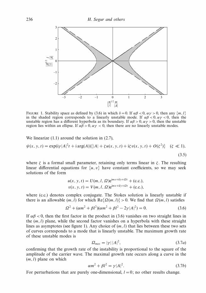
Figure 1. Stability space as defined by (3.6) in which δ = 0. If αβ < 0, αγ > 0, then any m, lin the shaded region corresponds to a linearly unstable mode. If αβ < 0, αγ < 0, then theunstable region has a different hyperbola as its boundary. If αβ > 0, αγ > 0, then the unstableregion lies within an ellipse. If αβ > 0, αγ < 0, then there are no linearly unstable modes.
We linearize (1.1) around the solution in (2.7),
ψ(x, y, t) = exp(iγ |A|2t + i arg(A))|A| + ζu(x, y, t) + iζv(x, y, t) + O(ζ 2) (ζ 1),
(3.5)
where ζ is a formal small parameter, retaining only terms linear in ζ . The resultinglinear differential equations for u, v have constant coefficients, so we may seeksolutions of the form
u(x, y, t) = U (m, l, Ω)eimx+ily+Ωt + (c.c.),
v(x, y, t) = V (m, l, Ω)eimx+ily+Ωt + (c.c.),
where (c.c.) denotes complex conjugate. The Stokes solution is linearly unstable ifthere is an allowable (m, l) for which ReΩ(m, l) > 0. We find that Ω(m, l) satisfies
Ω2 + (αm2 + βl2)(αm2 + βl2 − 2γ |A|2) = 0. (3.6)
If αβ < 0, then the first factor in the product in (3.6) vanishes on two straight lines inthe (m, l) plane, while the second factor vanishes on a hyperbola with these straightlines as asymptotes (see figure 1). Any choice of (m, l) that lies between these two setsof curves corresponds to a mode that is linearly unstable. The maximum growth rateof these unstable modes is
Ωmax = |γ | |A|2, (3.7a)
confirming that the growth rate of the instability is proportional to the square of theamplitude of the carrier wave. The maximal growth rate occurs along a curve in the(m, l) plane on which
αm2 + βl2 = γ |A|2. (3.7b)
For perturbations that are purely one-dimensional, l = 0; no other results change.
Stabilizing the Benjamin–Feir instability 237
4. Stability of a Stokes solution of (2.5)The solution of (2.5) corresponding to a spatially uniform plane wave was given in
(2.8). Its stability is the main theoretical result in this paper.
4.1. Linearized stability
Set
µ(x, y, t) = exp
iγ |A|2
(1 − e−2δt
2δ
)+ i arg(A)
× |A| + ζu(x, y, t) + iζv(x, y, t) + O(ζ 2), (4.1)
where ζ is a formal small parameter, substitute into (2.5), and retain only terms thatare linear in ζ . The result is
∂tv = α∂2xu + β∂2
yu + 2γ e−2δt |A|2u,
−∂tu= α∂2x v + β∂2
y v.
(4.2)
According to (2.3), all square-integrable solutions of (2.1) decay to zero as t → ∞.This overall decay has been factored out of (2.5), so the Stokes solution is unstable ifthe small perturbations (u, v) grow without bound relative to the constant |A|.
Without loss of generality, we seek solutions of (4.2) in the form
u(x, y, t) = U (t; m, l) eimx+ily + U ∗e−imx−ily ,
v(x, y, t) = V (t; m, l) eimx+ily + V ∗e−imx−ily .
Then (4.2) becomes
dV
dt= −(αm2 + βl2 − 2γ e−2δt |A|2)U, (4.3a)
dU
dt= (αm2 + βl2)V, (4.3b)
ord2U
dt2+ [(αm2 + βl2)(αm2 + βl2 − 2γ e−2δt |A|2)]U = 0. (4.3c)
Equation (4.3) is a Sturm–Liouville problem (cf. Ince 1956, chap. 10), so Sturmiantheory implies the following results:
(i) if [(αm2 + βl2)(αm2 + βl2 − 2γ e−2δt |A|2)] > 0, all solutions of (4.3) oscillate intime;
(ii) if [(αm2+βl2)(αm2+βl2−2γ e−2δt |A|2)] < 0, then (4.3) admits a growing solution.As long as [(αm2 + βl2)(αm2 + βl2 − 2γ e−2δt |A|2)] − C2 < 0, this solution grows atleast as fast as e|C|t .
Here is the fundamental reason for the difference in stability between the appro-priate Stokes solutions of (1.1) and (2.1). According to (4.3), at any fixed time, the setof (m, l) modes that can grow exponentially lies in a region like that shown in figure 1.However, the bounding hyperbola for (2.1) is defined by
αm2 + βl2 − 2γ e−2δt |A|2 = 0, (4.4)
so the region of instability shrinks as t increases, and any specific (m, l) mode remainsin this shrinking region only for a limited time. After that time, every solution of(4.3) for this (m, l) oscillates in time. Therefore, no (m, l) mode grows forever. Thispoint was recognized by Luther & McKinstrie (1990), Hasegawa & Kodama (1995),Karlsson (1995) and Mei & Hancock (2003).
238 H. Segur and others
Using standard iterative methods from the theory of ordinary differential equations(cf. Ince 1956, chap. 3), we can show that for any (m, l), any δ > 0 and any t 0, thesolution of (4.3) satisfies
|U (t; m, l)| √
|U (0; m, l)|2 + |V (0; m, l)|2 exp
|γ ||A|2
δ(1 − exp(−2δt))
,
(4.5)
|V (t; m, l)| √
|U (0; m, l)|2 + |V (0; m, l)|2 exp
|γ ||A|2
δ(1 − exp(−2δt))
.
Therefore, if δ > 0 then for all t 0, every (m, l) mode satisfies
|U (t)|2 + |V (t)|2 2[|U (0)|2 + |V (0)|2] exp
2|γ ||A|2
δ(1 − exp(−2δt))
. (4.6)
Finally, we may solve (4.2) in a rectangular domain, D, in the (x, y)-plane, withperiodic boundary conditions. We restrict our attention to initial conditions of (4.2)that satisfy ∫∫
D
[u2(x, y, 0) + v2(x, y, 0)] dx dy < ∆, (4.7a)
for some ∆ to be determined. Using Parseval’s relation (cf. Guenther & Lee 1988)and (4.6), it follows that for all t 0,∫∫
D
[u2(x, y, t) + v2(x, y, t)] dx dy < 2∆ exp
2|γ ||A|2
δ(1 − exp(−2δt))
. (4.7b)
However, u, v are the real and imaginary parts of the linearized perturbation of theStokes solution of (2.1). Therefore, for each ε > 0, if we choose
0 < ∆ 12ε exp
−2|γ | |A|2
δ
(4.8)
then it follows from (4.7) and (2.10) that the Stokes solution of (2.1) is linearly stable.This completes the proof of theorem 1.
Comments
(i) This proof applies for any choice of real constants α, β, γ in (2.1) or (2.5),provided δ > 0. Figure 1 requires αβ < 0, αγ > 0, but that restriction is not used inthe proof.
(ii) A similar proof applies for square-integrable perturbations in the whole (x, y)plane, if we impose on (2.1) or (2.5) vanishing boundary conditions at infinity.
(iii) Stability of the Stokes solution of (2.1) or (2.5) does not mean that sidebandmodes gain no energy from the carrier wave. Instead, it means that a sideband modecan gain at most a finite amount of energy. Typically, sidebands grow for a limitedtime, but (4.5) and (4.6) provide bounds on their total growth. If |γ | |A|2/δ 1, thisgrowth can be substantial; but even with substantial growth, the Stokes solution of(2.5) is still linearly stable: (4.8) requires only that ∆ be that much smaller.
(iv) Without dissipation, the Benjamin–Feir instability supplies energy from thecarrier wave to the sidebands until the sidebands have grown so large that their ownnonlinear interactions have become important. This process might still occur in thepresence of dissipation, but the analysis presented here shows that dissipation providesa second option. Namely, a sideband stops growing once dissipation has removedenough energy from the carrier wave to quench the instability for that sideband,according to (4.3). Thus, if the sideband has a small enough initial amplitude, then it
Stabilizing the Benjamin–Feir instability 239
stops growing before its own nonlinear interactions become important. If the ampli-tudes of all sidebands are small enough initially, then none of them grows very large, sothe Stokes wave solution of (2.1) is linearly stable. Then nonlinear interactions amongsidebands play no significant role. This is the physical significance of theorem 1.
4.2. Nonlinear stability
There are known problems in which linearized stability does not guarantee nonlinearstability (cf. Cherry 1926), so next we prove theorem 2, that the Stokes solution of(2.5) with periodic boundary conditions is nonlinearly stable. To do so, replace (4.1)with
µ(x, y, t) = exp
iγ |A|2
(1 − e−2δt
2δ
)+ i arg(A)
[|A| + u(x, y, t) + iv(x, y, t)],
substitute into (2.5), and retain all terms. Instead of (4.2), the result is
∂tv = α∂2xu + β∂2
yu + φ
u +
3u2 + v2
2|A| +(u2 + v2)u
2|A|2
, (4.9a)
−∂tu = α∂2x v + β∂2
y v + φ
uv
|A| +(u2 + v2)v
2|A|2
, (4.9b)
where
φ = 2γ e−2δt |A|2. (4.9c)
It follows from (4.9) that
∂t (u2 + v2) = 2α∂x(v∂xu − u∂xv) + 2β∂y(v∂yu − u∂yv) + 2φuv + φ
(u2 + v2)v
|A|
. (4.10)
Define λ(x, y, t) = u(x, y, t) + iv(x, y, t), so ∂xλ(x, y, t) = ∂xu(x, y, t)+ i∂xv(x, y, t),etc. Then denote
‖λ(t)‖22 =
∫∫D
[u2 + v2] dx dy, ‖∂xλ(t)‖22 =
∫∫D
[(∂xu)2 + (∂xv)2] dx dy, (4.11)
etc. We will also use
‖∂xλ(t)‖4 =
[∫∫D
[(∂xu)2 + (∂xv)2]2 dx dy
]1/4
,
and
‖λ(t)‖∞ =sup|u(x, y, t)|, |v(x, y, t)|
(x, y) ∈ D.
If u, v happen to be y-independent, then the y-integration in (4.11) is trivial.It follows from (4.10) and the Cauchy–Schwarz inequality that
d
dt
(‖λ‖2
2
) |φ|‖λ‖2
2 + |φ|∫∫
D
[(u2 + v2)
|v||A|
]dx dy. (4.12)
The integral in (4.12) represents the contribution from the nonlinear terms in (4.9).Neglecting the integral leads to a slightly improved form of (4.7b). Retaining theintegral in (4.12), we find
d
dt
(‖λ‖2
2
) |φ|‖λ‖2
2
[1 +
‖λ‖∞
|A|
]. (4.13)
240 H. Segur and others
A similar calculation leads to
d
dt
(‖∂xλ‖2
2
) |φ|‖∂xλ‖2
2 +2
|A| |φ|∫∫
D
[|2u(∂xu∂xv) + ((∂xv)2 − (∂xu)2)v|
]dx dy
+2
|A|2 |φ|∫∫
D
[|(u2 − v2)(∂xu∂xv) + ((∂xv)2 − (∂xu)2)uv|
]dx dy, (4.14)
so thatd
dt
(‖∂xλ‖2
2
) |φ|‖∂xλ‖2
2
1 +
4‖λ‖∞
|A| +4‖λ‖2
∞|A|2
. (4.15)
In the one-dimensional problem (i.e. ∂y ≡ 0), nonlinear stability follows from (4.13)and (4.15). To see this, define a Sobolev norm (Adams 1975):
‖λ(t)‖21,2 = ‖λ(t)‖2
2 + ‖∂xλ(t)‖22 =
∫D
[u2 + v2 + (∂xu)2 + (∂xv)2] dx. (4.16)
Then it follows from (4.13) and (4.15) that
d
dt
(‖λ‖2
1,2
) |φ|‖λ‖2
1,2
1 +
4‖λ‖∞
|A| +4‖λ‖2
∞|A|2
.
Hence, if there is a constant, N , such that ‖λ(t)‖∞ N < ∞ for all t 0, then byGronwall’s inequality (Coddington & Levinson 1955),
‖λ(t)‖21,2 ‖λ(0)‖2
1,2 exp
|φ(t))|
(1 +
2N
|A|
)2, (4.17a)
where
φ(t) =γ |A|2
δ(1 − e−2δt ). (4.17b)
However, it is known (Adams 1975, p. 97) that in one spatial dimension, there is aconstant C1, independent of λ, such that
‖λ‖∞ C1‖λ‖1,2. (4.18)
Then it follows from (4.17a) and (4.18) that for all t 0,
‖λ(t)‖21,2 < ε
provided
‖λ(0)‖21,2 < ∆ ε exp
−|γ ||A|2
δ
(1 +
2C1
√ε
|A|
)2. (4.19)
Therefore the Stokes solutions of (2.5) and of (2.1), both given in (2.8), are nonlinearlystable to small perturbations in one spatial dimension. This proves theorem 2 in onedimension. In two dimensions, the proof follows similar lines but is more complicatedbecause (4.18) no longer holds. See Appendix B for that proof.
5. Predictions of experimental observationsIn § 6, we describe experiments on nearly monochromatic waves of moderate
amplitude in deep water. The experiments were conducted to test the dissipative theorypresented here. A one-dimensional model is adequate to describe those experiments,so in this section we set ∂y ≡ 0 in (2.1) and in (2.5), and derive predictions of thedissipative model, to be compared with experimental data in § 6. The results obtained
Stabilizing the Benjamin–Feir instability 241
in this section are approximate, and they follow from (2.5). Alternatively, we canobtain predictions directly from (2.5) by integrating that equation numerically. Weuse both kinds of prediction in § 6.
In the experiments to be discussed, a spatially uniform one-dimensional wavetrainof moderate amplitude is perturbed by two wavetrains, each of small amplitude andeach travelling in the same direction as the carrier wave. One of these perturbationwavetrains has waves with frequency slightly higher than that of the carrier wave,while the other has a frequency slightly lower. For our experiments, the two frequencydifferences are equal, so the initial data for (1.1) or (2.1) have approximately the form
ψ(x, 0) = A + a1 eibx + a−1 e−ibx, (5.1)
where A, a1, a−1 can be complex, with |a1| |A|, |a−1| |A|, and b represents thefrequency difference between the carrier wave and either perturbation. The initialdata are prescribed at one end of a test section, and the evolution occurs as thewave propagates along the test section. (Recall that in § 3 we defined x to representclock-time, so b is a frequency in (5.1).)
5.1. The spectrum of the one-dimensional wave pattern
The data in (5.1) are periodic in x, so for either (1.1) or (2.1) with ∂y ≡ 0, the solutionthat evolves from these data must be periodic in x as well. Necessarily it has the form
ψ(x, t) = e−δt
∞∑−∞
an(t) einbx (δ 0), (5.2)
so the only frequency differences generated by nonlinear interactions are integermultiples of b. This effect can be seen in a spectral representation of the data at anyfixed ‘time’ (i.e. at any fixed location along the test section).
5.2. A weakly nonlinear theory
Solutions of (2.5) corresponding to (5.1) have the form µ(x, t) =∑∞
n=−∞ an(t) einbx;µ(x, t) is complex, so an(t) can be complex as well. In this representation, (2.6a, b)become
Mµ =
∞∑n=−∞
|an(t)|2 = const, (5.3a)
Pµ = 2b
∞∑n=−∞
n|an(t)|2 = const. (5.3b)
In addition, (2.5) reduces to an infinite set of coupled ODEs. For every integer n,
ian − α(nb)2an + γ e−2δt
∞∑m,p=−∞
∑amapa∗
m+p−n = 0. (5.4)
In our experiments, the initial data are rarely clean enough to satisfy (5.1) exactly.The theory we derive next applies under somewhat relaxed assumptions. Suppose
a0(t) = O(√
Mµ), a1(t) √
Mµ, a−1(t) = O(a1),
and for |n| > 1,
an(t)√Mµ
= O
((a1√Mµ
)|n|).
(5.5)
242 H. Segur and others
Rewrite (5.4) to reflect this ordering. For n= 0,
ia0 + γ e−2δt
[Mµa0 + a0
∞∑p=1
|ap|2 + |a−p|2 + 2a∗0
∞∑p=1
apa−p
]
+ γ e−2δt∑ ∞∑
m,p=1
(amapa∗m+p + a−ma−pa∗
−m−p)
+ γ e−2δt∑ ∞∑
m,p=1
2(a∗ma−pam+p + a∗
−mapa−m−p) = 0. (5.6a)
For n= 1,
ia1 − αb2a1 + γ e−2δt[2Mµa1 − |a1|2a1 + a2
0a∗−1
]+ 2γ e−2δt
∞∑p=1
(a∗0a−pap+1 + a0a
∗pap+1 + a0a−pa∗
−p−1)
+ γ e−2δt∑ ∞∑
m,p=1
(2a−ma∗pam+p+1 + a−ma−pa∗
−m−p−1)
+ γ e−2δt
[2
∞∑p=1
∞∑m=2
ama∗−pa1−m−p +
∑ ∞∑m,p=2
amapa∗m+p−1
]= 0, (5.6b)
etc. No approximations to (2.5) have been made to this point.For the remainder of this section, assume that (5.5) holds. Then it follows from
(5.3a) that Mµ = |a0|2 + O((a1)2), and (5.6a) becomes
ia0 + γ e−2δt [Mµa0] = O((a1)2), (5.7)
with the solution
a0(t) = A exp
iγMµ
2δ(1 − e−2δt )
+ O((a1)
2), (5.8a)
where A is a complex-valued constant. If an ≡ 0 for n =0, then Mµ = |a0|2 and (5.8a)becomes (2.8b). In what follows, we make use of (4.17b) and (4.9c). Then (5.8a)becomes
a0(t) = A eiφ/2 + O((a1)2). (5.8b)
Thus, at leading order in this weakly nonlinear theory, |a0(t)|2 = |A|2 = constant.
5.3. Evolution of the excited sideband
From (5.1), the excited sideband has the form [a1(t) eibx + a−1(t) e−ibx]. For small|a1(t)|, |a−1(t)|, these amplitudes evolve according to
ia1 − αb2a1 + φ[a1 + 1
2eiφ+2i argAa∗
−1
]= O((a1)
3),(5.9)
ia−1 − αb2a−1 + φ[a−1 + 1
2eiφ+2i argAa∗
1
]= O((a1)
3).
Define
c1(t) = a1(t) + a−1(t), s1(t) = a1(t) − a−1(t),
so that
[a1 eibx + a−1 e−ibx] = c1 cos(bx) + is1 sin(bx).
Stabilizing the Benjamin–Feir instability 243
Thus c1(t) represents the part of this sideband that is even in x, while s1(t) representsthe part that is odd in x. It follows from (5.9) that to O((a1)
3),
ic1 − αb2c1 + φ[c1 + 1
2eiφ+2i argAc∗
1
]= 0,
is1 − αb2s1 + φ[s1 − 1
2eiφ+2i argAs∗
1
]= 0.
(5.10)
Both c1(t) and s1(t) are complex-valued, so set c1(t) = [u1(t)+ iv1(t)] eiφ(t)/2+i argA, andobserve that u1(t), v1(t) satisfy (4.3a, b) with βl2 = 0, m = b in those equations.Similarly, set is1(t) = [U1(t) + iV1(t)] eiφ(t)/2+i argA and observe that U1(t), V1(t) alsosatisfy (4.3a, b) with βl2 = 0, m = b. It follows from these observations and (4.6) that
|a1(t)|2 12[|c1(0)|2 + |s1(0)|2] e2|φ(t)|, |a−1(t)|2 1
2[|c1(0)|2 + |s1(0)|2] e2|φ(t)|,
for as long as the linearized equations remain valid approximations. More preciseinformation about a1(t) and a−1(t) can be obtained by integrating (4.3) directly, as wedo in § 6.
Note that the symmetric (c1) and antisymmetric (s1) parts of this sideband can eachgrow for a while, but then must oscillate in time. If the initial seeded perturbationhappens to be even in x at t = 0 (so a−1(0) = a1(0)), then it remains even as it evolves.If it has any initial asymmetry, then this asymmetry can also grow, but then mustoscillate.
Specifically, each of (1.1), (2.1) and (2.5) is invariant under x → −x. Even so, ifthe initial data for these equations are asymmetric in x, then that asymmetry willtypically grow during the growth phase of the evolution. We show in § 6 that thiskind of asymmetric growth commonly occurs in practice, and that (2.5) describes theasymmetric growth accurately, even though (2.5) is symmetric x → −x.
5.4. Evolution of other sidebands
Nonlinear interactions of the first sideband with itself and with the carrier wavegenerate the second sideband, [a2(t) e2ibx + a−2(t) e−2ibx]. If (5.5) holds, then theamplitudes of this sideband satisfy
ia2 − 4αb2a2 + φ[a2 + 1
2eiφ+2i argAa∗
−2
]+ γ e−2δt
[2a0a1a
∗−1 + a∗
0a21
]= O((a1)
4),
ia−2 − 4αb2a−2 + φ[a−2 + 1
2eiφ+2i argAa∗
2
]+ γ e−2δt
[2a0a−1a
∗1 + a∗
0a2−1
]= O((a1)
4).
(5.11)
As with (5.9), define
c2(t) = a2(t) + a−2(t), s2(t) = a2(t) − a−2(t),
and set
c2 = [u2 + iv2] eiφ/2+i argA, is2 = [U2 + iV2] eiφ/2+i argA.
Then (5.11) provides two pairs of real-valued equations:
u2 − 4αb2v2 +φ
2|A| (u1v1 − U1V1) = 0, (5.12a)
−v2 − 4αb2u2 + φu2 +φ
4|A|(3u2
1 + v21 − 3U 2
1 − V 21
)= 0, (5.12b)
and
−V 2 − 4αb2U2 + φU2 +φ
2|A| (3u1U1 + v1V1) = 0, (5.12c)
U 2 − 4αb2V2 +φ
2|A| (u1V1 + v1U1) = 0. (5.12d)
244 H. Segur and others
With φ(t), u1(t), v1(t), U1(t), V1(t) known (from having integrated (4.3) twice),(5.12) contains forced linear equations that can be solved explicitly. It followsfrom (5.12) that even if a2(0) = 0 = a−2(0) initially, these amplitudes grow until|a2(t)| = O(|a1(t)|2/
√Mµ) and |a−2(t)| = O(|a1(t)|2/
√Mµ), as asserted in (5.5). In fact,
we can show that
|c2(t)| 2
|A| [|c1(0)|2 + |s1(0)|2] e|φ|(1 − e−|φ|/2) + |c2(0)| e|φ|/2,
|s2(t)| 2
|A| [|c1(0)|2 + |s1(0)|2] e|φ|(1 − e−|φ|/2) + |s2(0)| e|φ|/2.
More precise information about a2(t), a−2(t) can be obtained by integrating (5.12)directly.
We can continue in this way to obtain weakly nonlinear approximations for all ofthe amplitudes identified in (5.2). The next set of sidebands satisfies
ia3 − 9αb2a3 + φ[a3 + 1
2eiφ+2i arg(A)a∗
−3
]+ 2γ e−2δt
[a0a1a
∗−2 + a∗
0a1a2 + a0a∗−1a2 + 1
2a2
1a∗−1
]= O((a1)
5), (5.13a)
and
ia−3 − 9αb2a−3 + φ[a−3 + 1
2eiφ+2i arg(A)a∗
3
]+ 2γ e−2δt
[a0a−1a
∗2 + a∗
0a−1a−2 + a0a∗1a−2 + 1
2a2
−1a∗1
]= O((a1)
5). (5.13b)
We omit calculations for higher modes, because amplitudes smaller than O(a3(t)) weretoo small to measure accurately in our experiments.
5.5. Higher-order evolution of the carrier wave
According to (5.8), |a0(t)| is constant at leading order. However, from (5.3a), the othermodes cannot grow significantly unless a0(t) loses energy to these modes. This transferof energy from the carrier wave to the sidebands occurs at O((a1)
2), as we show next.A better approximation to (5.6a) than (5.7) is
ia0 + γ e−2δt [Mµa0 + a0(|a1|2 + |a−1|2) + 2a∗0a1a−1)] = O((a1)
4).
Represent a1(t) and a−1(t) as before, but now set a0(t) = |A| + u0(t) + iv0(t)× eiφ(t)/2+i arg(A, where we expect (u0, v0) = O((a1)
2). The result is:
u0 +φ
2√
Mµ
(u1v1 + U1V1) = 0, −v0 +φ
2√
Mµ
(u2
1 + U 21
)= 0. (5.14)
Comparing (5.14a) with (5.10), we can show that
u0(t) = u0(0) +1
4√
Mµ
[|c1(0)|2 + |s1(0)|2 − |c1(t)|2 − |s1(t)|2],
v0(t) = v0(0) +1
2√
Mµ
∫ t
0
(u2
1 + U 21
)φ dτ. (5.15)
We can choose A so that u0(0) = 0 = v0(0). Then
|a0(t)|2 = |A|2 + 12(|c1(0)|2 − |c1(t)|2) + 1
2(|s1(0)|2 − |s1(t)|2) + O((a1)
4).
Alternatively, we can solve (5.3a) for |a0(t)|2 to obtain
|a0(t)|2 = Mµ −[
|a1(t)|2 + |a−1(t)|2 + |a2(t)|2 + |a−2(t)|2) + O
(a6
1
M2µ
)]. (5.16)
Stabilizing the Benjamin–Feir instability 245
5.6. Evolution of the second harmonic of the carrier wave
Equations (2.1) and (1.1) each describe approximately the evolution of a nearlymonochromatic wavetrain of moderate amplitude, with and without dissipation,respectively. Each model is designed to be accurate for waves with frequency nearthat of the carrier wave. The second harmonic of the carrier wave has a frequencytwice that of the carrier wave, so it lies outside the region of validity of either model.Even so, the derivation of either model from the original physical problem impliesa necessary relation between the amplitude of the harmonic and that of the carrierwave. For waves in deep water, this relation is given in (3.2). In this way, the evolutionof the second harmonic is controlled by the evolution of the carrier wave.
In the problem under consideration, at leading order
ψ(x, t) = e−δt[Aeiφ/2 + o(1)
].
When combined with (3.2), this implies the dominant behaviour of the secondharmonic:
‖ψ2(x, t)‖ ∼ e−2δtconst. (5.17)
Thus, (2.1) predicts that as the carrier wave decays, its second harmonic also decays,with a decay rate twice that of the carrier wave.
In fact, (3.2) provides more information about this harmonic. Once the amplitudeof the carrier wave has been measured, then (3.2) predicts the amplitude of the secondharmonic, with no adjustable parameters. Lake & Yuen (1977) emphasized this pointin comparing their experiments with the B–F theory. To see this, represent both sidesof (3.2) in Fourier series in x, and single out the mean term of each side. The result is
ah(t) =
(1 + τk2
0/g
1 − 2τk20/g
)k0
[a2
0(t) + 2a1(t)a−1(t) + O
(a4
1
Mµ
)], (5.18)
where ah(t) is the complex amplitude of the second harmonic. This specifies ah(t)completely, to this order of approximation.
5.7. The most unstable wavenumber
In the absence of dissipation, the growth rate of each unstable wavenumber is givenby (3.5), so we can find a most unstable wavenumber and a maximal growth rate, asshown in (3.6). The situation changes if δ > 0, because the most unstable wavenumberat one instant of time ceases to be the most unstable at a later instant. Accordingto (4.3), all modes stop growing eventually, so we can ask for the wavenumberwith the maximal total growth. Even this can be ambiguous for an experiment oflimited duration, because the maximal total growth can depend on the duration ofthe experiment (i.e. the length of the test section). Generally, the concept of a mostunstable wavenumber is unambiguous and easily testable in an experiment withoutdissipation, but less well-defined in an experiment with dissipation.
5.8. Frequency downshifting
In their experimental study of waves in deep water, Lake et al. (1977) discoveredfrequency downshifting, a process in which the frequency of the carrier wave slowlyshifts to lower values as the waveform evolves. Afterwards, frequency downshiftingwas also observed and explained in optics (Gordon 1986). To our knowledge,downshifting cannot be explained by either (1.1) or (2.1), with or without (5.5). Thesemodels are too simple to explain this effect. We intend to report on downshifting ina subsequent paper.
246 H. Segur and others
6. Experimental tests of the dissipative theoryOur main point, that any amount of dissipation (of the correct kind) stabilizes
the Benjamin–Feir instability for waves of moderate amplitude, contradicts well-established beliefs with regard to water waves, to optics and to plasmas. Therefore,we conducted laboratory experiments on waves in deep water, to see how well (2.1)describes the evolution of nearly monochromatic waves of moderate amplitude, asthese waves propagate down a long wave tank. In this section, we describe both theexperiments and their comparisons with the predictions of (2.1), given in § 5. We alsocompare the experimental results with predictions from two non-dissipative models,(1.1) and Dysthe’s (1979) equation.
6.1. Experimental apparatus and procedures
The experimental apparatus comprised a wave channel, wavemaker, wave gauges,computer systems and water supply.
The wave channel is 43 ft long and 10 in wide with glass bottom and sidewalls. Atone end is a sanded-glass beach to minimize reflections. Its toe is at 32.8 ft from thewavemaker. At the other end is a plunger-type wavemaker that oscillates vertically andhas an exponential (E) cross-section that spans the width of the tank. The idea behindthe E-plunger is to mimic more closely the (linearized) velocity field of a deep-waterwave, which falls off exponentially in the vertical. The E-plunger used herein falls offwith the wavenumber of a 3.33 Hz wave, the carrier wave used in these experiments.The wavemaker is driven by a motor under digital control using dual closed-loopfeedbacks (position and velocity) to follow faithfully the command signals of position,velocity and time. This is the most precise linear motion technology available today.
For the experiments in this section ηw , the displacement of the wavemaker in theundisturbed water level, is prescribed to be a modulated sine wave
ηw(T ) = 2a0 sin(ω0T )[1 + 2r sin(ωpT + ϕ)], (6.1)
where the subscripts ‘0’ and ‘p’ indicate carrier and perturbation modes, r = ap/a0 isthe ratio of the perturbation amplitude to the carrier wave amplitude, and an denotesa real-valued measured wave amplitude. We note that with the definition of Fourieramplitudes implied by (5.2), the crest-to-trough amplitude of an oscillatory wave is2|an|. The vertical velocity of the wavemaker is prescribed as the time-derivative ofηw . In this way, we seeded a particular perturbation mode in each experiment. If wedid not seed modes for carrier waves of moderate amplitude, then the perturbationdid not grow enough in our test section to observe measurable growth. If we did notseed modes for carrier waves of large amplitude, then perturbations grew measurably,but Mµ and/or Pµ was not conserved.
To compare measurements with predictions from the theory, note that (6.1) can bewritten as
ηw(T ) = eiω0T [−ia0 − apeiωpT +iϕ + ape−iωpT −iϕ]
+ e−iω0T [ia0 − ape−iωpT −iϕ + apeiωpT +iϕ].
This is consistent with the notation in (3.1) and (5.1) if we identify
εb =ωp
ωo
, (6.2a)
εψ(x, 0) = [−ia0 − apeibx+iϕ + ape−ibx−iϕ]. (6.2b)
Stabilizing the Benjamin–Feir instability 247
The wavegauge is a non-intrusive capacitance-type gauge that spans 12.7 cm of thewidth of the tank and 6 mm in the direction of wave propagation. It was calibrateddynamically by oscillating it at the carrier wave frequency and it has a remarkablylinear calibration that remains constant over a period of days. Time series of watersurface displacement were recorded at sampling rates of either 300 or 350 Hz for 25 susing LabView software and National Instruments hardware.
In all of the experiments discussed in this section, the wavemaker was oscillatedwith the motion (6.1). One set of experiments consisted of N experiments – typically,N = 12 or 14. In the nth experiment of the set (n= 1, 2, . . . , N), the wavegaugewas fixed at a distance of Xn = 128 + 50(n − 1) cm from the wavemaker. A timeseries of water surface displacement at that point was measured. The n=1 locationwas chosen to be out of the regime of evanescent waves near the wavemaker. Wecomputed the Fourier transform of the nth time series to obtain the complex Fourieramplitudes with a frequency resolution of ± 0.27 rad s−1 or ± 0.04 Hz. From theFourier transforms of each of the n time series, we evaluated: (i) Mµ from (5.3a);(ii) Pµ from (5.3b); (iii) a0, the Fourier amplitude of the carrier wave at frequencyω0; (iv) ah, the Fourier amplitude of its harmonic at frequency 2ω0; (v) a1, a−1, theFourier amplitudes of the two seeded sidebands, at frequencies ω0 ± ωp; (vi) a2, a−2,the Fourier amplitudes of the second sidebands, at frequencies ω0 ± 2ωp; and (vi) a3,a−3, the Fourier amplitudes of the third sidebands, at frequencies ω0 ± 3ωp .
Note that each of these Fourier amplitudes is complex-valued. Both the magnitudeand phase of each Fourier amplitude, measured at the n= 1 location, are requiredas initial data for the predictive differential equations like (4.3) and (5.12). In thecomparisons that follow, we plot only magnitudes of Fourier amplitudes, like |a0|, butboth magnitude and phase are required for a complete theory.
The validity of the exponential decay model is crucial for the validity of (2.1); thus,we also conducted experiments using unseeded wavetrains that varied wave amplitudeand water surface age, to determine how the waves decay. These experiments arediscussed in Appendix A. Our procedure for the experiments in this section was toclean the tank with alcohol before filling it to a depth of h > 20 cm. A brass rodthat spans the width of the tank and is mounted on a carriage above the tank wasskimmed along the surface, scraping the surface film to the end of the tank. Therethe film was vacuumed with a wet vac. The wet vac was used further to vacuum thewater surface throughout the tank until the depth was h = 20 cm as measured by apoint gauge mounted above the tank.
The experiments in Appendix A show that the waves decayed approximatelyexponentially and that the decay rate varied with surface age. However, the decayrate was essentially constant during the first two hours after cleaning the watersurface. Thus, before each set of N experiments, the surface was cleaned as describedabove. The tank was allowed to settle for 10 min between the n and n+1 experiments,and the set of N experiments was conducted within about a 2 h period after cleaningthe surface.
We obtained the value for δ, the measured spatial decay rate, in three waysand compared the results: (i) we found the L2 norm of the nth time series bynumerically integrating the data, and then fit an exponential through those results;(ii) we computed values for Mµ of the nth time series from (5.3a) by summing theFourier coefficients for all of the modes resolved in the nth time series, and then fitan exponential through those results; and (iii) we computed values for Mµ of thenth time series from (5.3a) by summing the Fourier coefficients for a band of modesaround the carrier, and then fit an exponential through those results. In all cases,
248 H. Segur and others
ω0/2π (Hz) ωp/2π (Hz) 2a0(0) (cm) (|a−1| + |a1|)/(2|a0|)−1
3.33 0.17 −0.116 + 0.183 i 0.11
2u1 (0) (cm) 2v1(0) (cm) 2U1 (0) (cm) 2V1 (0) (cm)−0.032 0.051 −0.009 0.007
2u2(0) (cm) 2v2(0) (cm) 2U2(0) (cm) 2V2(0) (cm)0.000 −0.006 0.002 −0.009
Re(2a3(0)) Im(2a3(0)) Re(2a−3(0)) Im(2a−3(0))0.001 0.001 −0.001 0.000
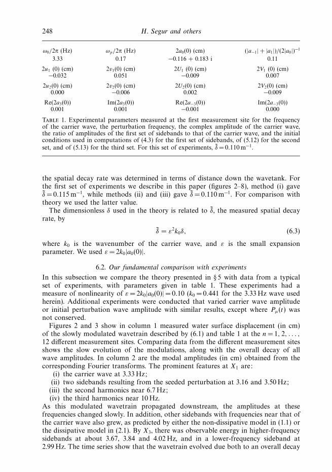
Table 1. Experimental parameters measured at the first measurement site for the frequencyof the carrier wave, the perturbation frequency, the complex amplitude of the carrier wave,the ratio of amplitudes of the first set of sidebands to that of the carrier wave, and the initialconditions used in computations of (4.3) for the first set of sidebands, of (5.12) for the secondset, and of (5.13) for the third set. For this set of experiments, δ = 0.110 m−1.
the spatial decay rate was determined in terms of distance down the wavetank. Forthe first set of experiments we describe in this paper (figures 2–8), method (i) gaveδ =0.115 m−1, while methods (ii) and (iii) gave δ =0.110 m−1. For comparison withtheory we used the latter value.
The dimensionless δ used in the theory is related to δ, the measured spatial decayrate, by
δ = ε2k0δ, (6.3)
where k0 is the wavenumber of the carrier wave, and ε is the small expansionparameter. We used ε = 2k0|a0(0)|.
6.2. Our fundamental comparison with experiments
In this subsection we compare the theory presented in § 5 with data from a typicalset of experiments, with parameters given in table 1. These experiments had ameasure of nonlinearity of ε = 2k0|a0(0)| = 0.10 (k0 = 0.441 for the 3.33 Hz wave usedherein). Additional experiments were conducted that varied carrier wave amplitudeor initial perturbation wave amplitude with similar results, except where Pµ(t) wasnot conserved.
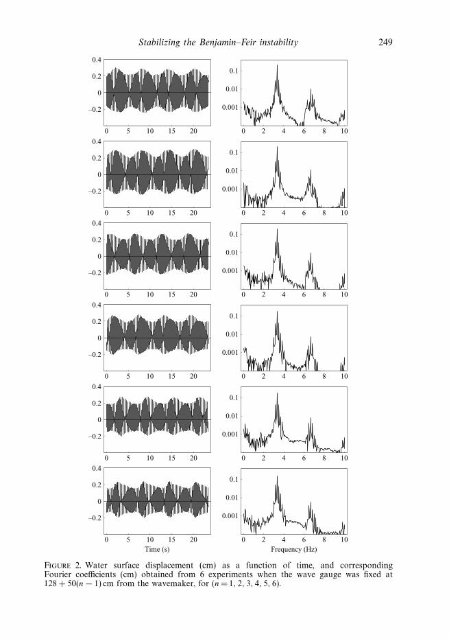
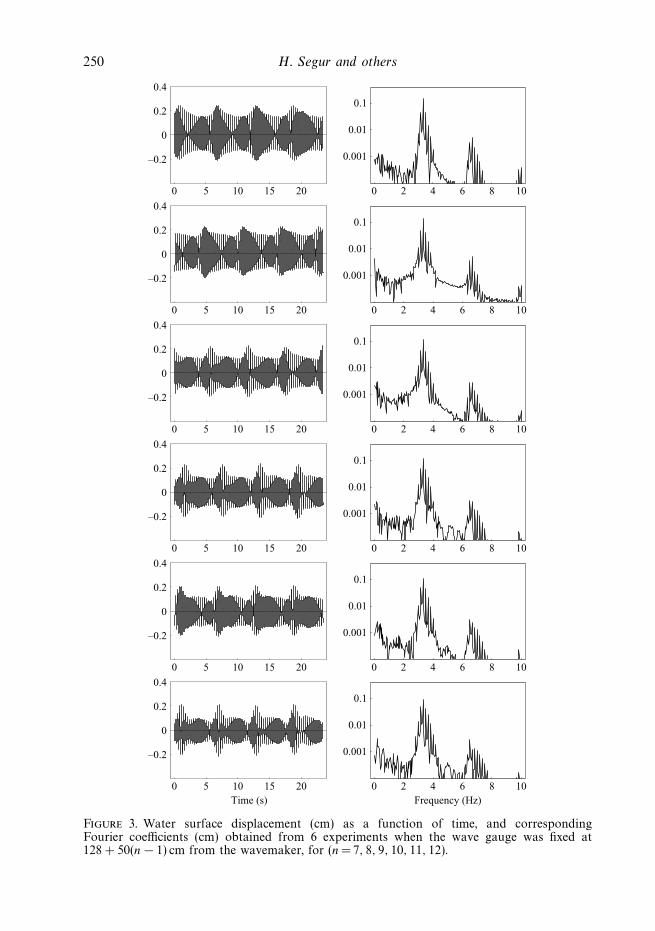
Figures 2 and 3 show in column 1 measured water surface displacement (in cm)of the slowly modulated wavetrain described by (6.1) and table 1 at the n= 1, 2, . . . ,
12 different measurement sites. Comparing data from the different measurement sitesshows the slow evolution of the modulations, along with the overall decay of allwave amplitudes. In column 2 are the modal amplitudes (in cm) obtained from thecorresponding Fourier transforms. The prominent features at X1 are:
(i) the carrier wave at 3.33 Hz;(ii) two sidebands resulting from the seeded perturbation at 3.16 and 3.50 Hz;(iii) the second harmonics near 6.7 Hz;(iv) the third harmonics near 10 Hz.
As this modulated wavetrain propagated downstream, the amplitudes at thesefrequencies changed slowly. In addition, other sidebands with frequencies near that ofthe carrier wave also grew, as predicted by either the non-dissipative model in (1.1) orthe dissipative model in (2.1). By X3, there was observable energy in higher-frequencysidebands at about 3.67, 3.84 and 4.02 Hz, and in a lower-frequency sideband at2.99 Hz. The time series show that the wavetrain evolved due both to an overall decay
Stabilizing the Benjamin–Feir instability 249
0 5 10 15 20
–0.2
0
0.2
0.4
0 2 4 6 8 10
0.001
0.01
0.1
0 5 10 15 20
–0.2
0
0.2
0.4
0 2 4 6 8 10
0.001
0.01
0.1
0 5 10 15 20
–0.2
0
0.2
0.4
0 2 4 6 8 10
0.001
0.01
0.1
0 5 10 15 20
–0.2
0
0.2
0.4
0 2 4 6 8 10
0.001
0.01
0.1
0 5 10 15 20
–0.2
0
0.2
0.4
0 2 4 6 8 10
0.001
0.01
0.1
0 5 10 15 20
–0.2
0
0.2
0.4
0 2 4 6 8 10
0.001
0.01
0.1
Time (s) Frequency (Hz)
Figure 2. Water surface displacement (cm) as a function of time, and correspondingFourier coefficients (cm) obtained from 6 experiments when the wave gauge was fixed at128 + 50(n − 1) cm from the wavemaker, for (n= 1, 2, 3, 4, 5, 6).
250 H. Segur and others
0 5 10 15 20
–0.2
0
0.2
0.4
0 2 4 6 8 10
0.001
0.01
0.1
0 5 10 15 20
–0.2
0
0.2
0.4
0 2 4 6 8 10
0.001
0.01
0.1
0 5 10 15 20
–0.2
0
0.2
0.4
0 2 4 6 8 10
0.001
0.01
0.1
0 5 10 15 20
–0.2
0
0.2
0.4
0 2 4 6 8 10
0.001
0.01
0.1
0 5 10 15 20
–0.2
0
0.2
0.4
0 2 4 6 8 10
0.001
0.01
0.1
0 5 10 15 20
–0.2
0
0.2
0.4
0 2 4 6 8 10
0.001
0.01
0.1
Time (s) Frequency (Hz)
Figure 3. Water surface displacement (cm) as a function of time, and correspondingFourier coefficients (cm) obtained from 6 experiments when the wave gauge was fixed at128 + 50(n − 1) cm from the wavemaker, for (n= 7, 8, 9, 10, 11, 12).
Stabilizing the Benjamin–Feir instability 251
0 100 200 300 400 500X (cm) X (cm)
0.01
0.02
0.03(a) (b)M
µ (
cm2 )
0 100 200 300 400 500
–0.002
0
0.002
0.004
Pµ (
cm2
s–1)
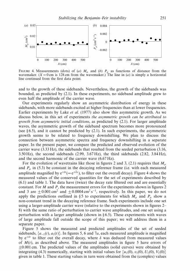
Figure 4. Measurements (dots) of (a) Mµ and (b) Pµ as functions of distance from thewavemaker. (X = 0 cm is 128 cm from the wavemaker.) The line in (a) is simply a horizontalline continued from the first data point.
and to the growth of these sidebands. Nevertheless, the growth of the sidebands wasbounded, as predicted by (2.1). In these experiments, no sideband amplitude grew toeven half the amplitude of the carrier wave.
Our experiments regularly show an asymmetric distribution of energy in thesesidebands, with more sidebands excited at higher frequencies than at lower frequencies.Earlier experiments by Lake et al. (1977) also show this asymmetric growth. As wediscuss below, in this set of experiments the asymmetric growth can be attributed togrowth from asymmetric initial conditions, as predicted by (2.1). For larger amplitudewaves, the asymmetric growth of the sideband spectrum becomes more pronounced(see § 6.5), and it cannot be predicted by (2.1). In such experiments, the asymmetricgrowth seems to be related to frequency downshifting. We plan to discuss theconnection between asymmetric spectra and frequency downshifting in a separatepaper. In the present paper, we compare the predicted and observed evolution of thecarrier wave (3.33 Hz), the sidebands that resulted from the seeded perturbation (3.16,3.50 Hz), the second sidebands (2.99, 3.67 Hz), the third sidebands (2.82, 3.84 Hz),and the second harmonic of the carrier wave (6.67 Hz).
For the evolution of wavetrains like those in figures 2 and 3, (2.1) requires that Mµ
and Pµ in (5.3) be constant in the decaying reference frame (i.e. with each measured
amplitude magnified by e+δt (= e+δx), to filter out the overall decay). Figure 4 shows themeasured values of the conserved quantities for the set of experiments described by(6.1) and table 1. The data have (twice) the decay rate filtered out and are essentiallyconstant. For M and P , the measurement errors for the experiments shown in figures 2and 3 are ± 0.001 cm2 and ± 0.0004 cm2 s−1, respectively. In this paper, we do notapply the predictions outlined in § 5 to experiments for which Mµ and Pµ show anon-constant trend in the decaying reference frame. Such experiments include one setusing a larger-amplitude carrier wave (relative to the experiments shown in figures 2–8) with the same ratio of perturbation to carrier wave amplitudes, and one set using aperturbation with a larger amplitude (shown in § 6.5). These experiments with wavesof large amplitude fall outside the scope of this paper; we will address them in aseparate paper.
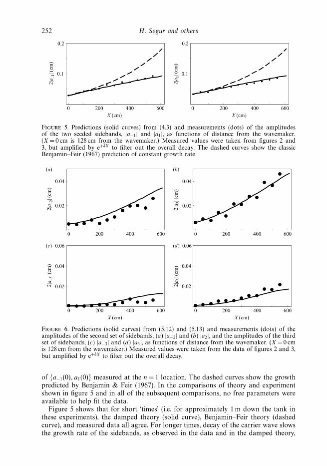
Figure 5 shows the measured and predicted amplitudes of the set of seededsidebands, a−1(t), a1(t). In figures 5, 6 and 7a, each measured amplitude is magnifiedby e+δt to filter out the overall decay, where δ was deduced from measured valuesof M(t), as described above. The measured amplitudes in figure 5 have errors of±0.001 cm. The predicted values of the amplitudes (solid curves) were obtained byintegrating (4.3) numerically, starting with initial values for u1(0), v1(0), U1(0), V1(0)given in table 1. These starting values in turn were obtained from the (complex) values
252 H. Segur and others
0 200 400 600X (cm) X (cm)
0.1
0.2
2|a –
1| (
cm)
2|a 1
| (cm
)
0 200 400 600
0.1
0.2
Figure 5. Predictions (solid curves) from (4.3) and measurements (dots) of the amplitudesof the two seeded sidebands, |a−1| and |a1|, as functions of distance from the wavemaker.(X = 0 cm is 128 cm from the wavemaker.) Measured values were taken from figures 2 and3, but amplified by e+δX to filter out the overall decay. The dashed curves show the classicBenjamin–Feir (1967) prediction of constant growth rate.
0 200 400 600
0.02
0.04
(a) (b)
2|a –
2| (
cm)
2|a 2
| (cm
)
0 200 400 600
0.02
0.04
(c) (d)
0 200 400 600X (cm) X (cm)
0.04
0.02
0.06
2|a –
3| (
cm)
2|a 3
| (cm
)
0 200 400 600
0.04
0.02
0.06
Figure 6. Predictions (solid curves) from (5.12) and (5.13) and measurements (dots) of theamplitudes of the second set of sidebands, (a) |a−2| and (b) |a2|, and the amplitudes of the thirdset of sidebands, (c) |a−3| and (d) |a3|, as functions of distance from the wavemaker. (X = 0 cmis 128 cm from the wavemaker.) Measured values were taken from the data of figures 2 and 3,but amplified by e+δX to filter out the overall decay.
of a−1(0), a1(0) measured at the n= 1 location. The dashed curves show the growthpredicted by Benjamin & Feir (1967). In the comparisons of theory and experimentshown in figure 5 and in all of the subsequent comparisons, no free parameters wereavailable to help fit the data.
Figure 5 shows that for short ‘times’ (i.e. for approximately 1 m down the tank inthese experiments), the damped theory (solid curve), Benjamin–Feir theory (dashedcurve), and measured data all agree. For longer times, decay of the carrier wave slowsthe growth rate of the sidebands, as observed in the data and in the damped theory,
Stabilizing the Benjamin–Feir instability 253
(a) (b)
0 200 400 600X (cm) X (cm)
0.4
0.3
0.2
0.1
0.5
0.020
0.015
0.010
0.005
0.0252|
a 0| (
cm)
2|a h
| (cm
)
0 200 400 600
Figure 7. Results for the (a) carrier wave amplitude and (b) its second harmonic as functionsof distance from the wavemaker. (X = 0 cm is 128 cm from the wavemaker.) The solid curve in(a) is the prediction from (5.16); the dots are the measured Fourier amplitudes at the carrierwave frequency, but amplified by e+δX . The solid curve in (b) is the prediction from (5.18).The dots are the measured Fourier amplitudes at twice the carrier wave frequency, amplifiedby e+2δX as required by (5.17).
but not in the undamped theory. Recall that the undamped theory is being comparedto data that has had the damping factored out. So, correcting the inviscid growth rateby subtracting the decay rate from it is inadequate for these waves.
Over the duration of these experiments, the damped theory predicts the measuredgrowth of the sidebands from their starting values with reasonable accuracy. Equation(4.3) predicts that this growth must eventually stop completely. Continuing thecomputation of (4.3) beyond 6 m, we find that |a−1(t)| and |a1(t)| would have achievedmaximum amplitudes of about 0.18 cm, or about 5.5 times their initial amplitudes,at about 10.7 m downstream from the wavepaddle. We ended our experiments beforethat distance to minimize the effects of reflections from the beach. As a result, we didnot observe the bound on growth in this experiment, but we do see it in a second setof experiments, shown in figure 9.
Figure 6 shows the growth of the next two sets of sidebands, a−2, a2, a−3, a3.None of these sidebands was seeded, so they started with smaller amplitudes thana−1, a1, and they remained smaller. The predicted values for a−2, a2 were obtainedby integrating (5.12) numerically, while the predictions for a−3, a3 were obtained byintegrating (5.13). In all cases, the starting (complex) values were taken from datameasured at the n= 1 location.
As in figure 5, the damped theory predicts the observed data over the durationof the experiment with good accuracy, and with no free parameters. The predictionsfor all six sidebands are in fairly good agreement with the data, which have errorsof ±0 .001 cm. Note that |a2(t)| grows nearly twice as much as |a−2(t)| during theexperiments, and that (2.5) accurately predicts this asymmetric growth. Equation (2.5)is symmetric under x → −x, but figure 6 shows that (2.5) admits solutions withgrowing asymmetry. The initial data a−2(0), a2(0) must be asymmetric, and thosemodes must be in the unstable region for a time. Then the asymmetric part of thesolution grows approximately exponentially, for a while. Note also that a−3, a3 areasymmetric, but the asymmetry is less pronounced. According to (2.5), the a−3, a3modes lay outside the unstable region for the entire experiment, so these two modesgrew asymmetrically only because of asymmetric forcing by a−1, a1 and a−2, a2.
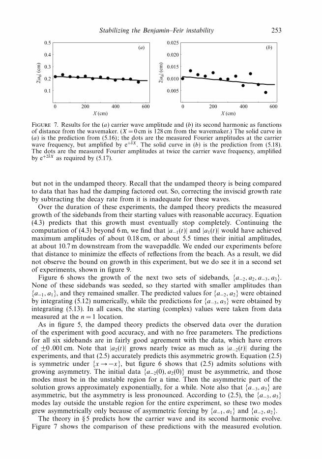
The theory in § 5 predicts how the carrier wave and its second harmonic evolve.Figure 7 shows the comparison of these predictions with the measured evolution.
254 H. Segur and others
Figure 7(a) shows the measured values of the carrier wave amplitude obtained fromthe Fourier transforms, with the overall decay rate filtered out. This amplitude variesslowly in this reference frame as it loses energy to the sidebands, as described by(5.16). The curve in figure 7(a) is from (5.16), using values for the sidebands given bythe computed solutions of (4.3) and (5.12).
Figure 7(b) shows the measured and predicted evolution of the second harmonic ofthe carrier wave. Recall from (5.17) that the second harmonic decays with twice thedecay rate of the carrier wave. Thus, twice the usual decay rate has been factored outin figure 7(b). The dots in figure 7(b) are the measured amplitudes of the harmonic,magnified by e2δt . The curve shows the evolution of the harmonic predicted by (5.18),using the computed solutions of (4.3) and (5.15) with u0(0) = v0(0) = 0. Thus, the curvetakes into account the evolution of the carrier wave and the first set of sidebands.
Note that the vertical scale in figure 7(b) is finer than that in figure 7(a); thus,figure 7(b) shows that (3.2) predicts the evolution of the harmonic quite accurately.Lake & Yuen (1977) found that (3.2) did not predict accurately the measurements intheir experiments, but we found no such problems.
6.3. Comparisons with other theories
Figures 4–7 show that (2.1) predicts all the easily measured features of the data shownin figures 2 and 3 with good accuracy, using no adjustable parameters. Even so, thisgood agreement does not rule out the possibility that another theory might alsopredict these data accurately. For example, it is known that the initially exponentialgrowth rate, predicted by Benjamin & Feir (1967) and shown in figure 5, can last onlyuntil nonlinear interactions among sidebands become important. For longer times,(1.1) predicts that the growth of the seeded sidebands, a, a1, must diminish as thesegrowing modes begin to lose energy to higher sidebands. Thus even with no damping(δ = 0), a nonlinear theory like (1.1) also predicts that the initially vigorous growth ofunstable sidebands must eventually slow down, consistent with the behaviour shownin figure 5. In terms of the behaviour of a−1, a1, the differences between the twotheories are that:
(i) the mechanism for the slowing down is different (nonlinear interactions for (1.1)vs. damping of the carrier wave for (2.1)); and
(ii) the time scales on which this slowing down occurs are typically different.Dysthe’s (1979) model could also be used to predict the evolution shown in figures 2
and 3. He derived his higher-order correction to (1.1) in order to predict the behaviourof nonlinear events more accurately. In the form given by Lo & Mei (1985), usingthe notation given herein, Dysthe’s model in one spatial dimension can be written as
i∂tψ + α∂2xψ + γ |ψ |2ψ + 8iεγ |ψ |2∂xψ − 4εγ ∂xφ(|ψ |2)ψ = 0, (6.4)
where
∂xφ(f ) = − 1
4π
∫|k|f (k, t) eikx dk, f (x, t) =
1
2π
∫f (k, t) eikx dk,
α, γ were given in § 3, and ε = 2k0|a0(0)|. Lo & Mei (1985) showed that (6.4) predictsthe evolution of some narrow-banded wave packets in deep water more accuratelythan does (1.1).
Figure 8 repeats the data shown in figures 5, 6 and 7, showing the evolutionof a0, a−1, a1, a−2, a2, a−3, a3 as functions of time, with each measured amplitudemagnified by e+δt to factor out the overall decay. We have also plotted the predictedevolution of each Fourier amplitude, according to (1.1), (2.1) in the form of (2.5), and
Stabilizing the Benjamin–Feir instability 255
0 200 400 600
0.06
0.09
0.03
0.12
0.06
0.09
0.03
0.12(b) (c)
2|a –
1| (
cm)
2|a 1
| (cm
)
0 200 400 600
(d ) (e)
0 200 400 600
0.05
0.10
0.05
0.10
2|a –
2| (
cm)
2|a 2
| (cm
)
0 200 400 600
( f ) (g)
0 200 400 600X (cm) X (cm)
0.05
0.10
2|a –
3| (
cm)
2|a 3
| (cm
)
0 200 400 600
0.05
0.10
(a)
0 200 400 600X (cm)
0.3
0.2
0.4
0.1
0.5
2|a 0
| (cm
)
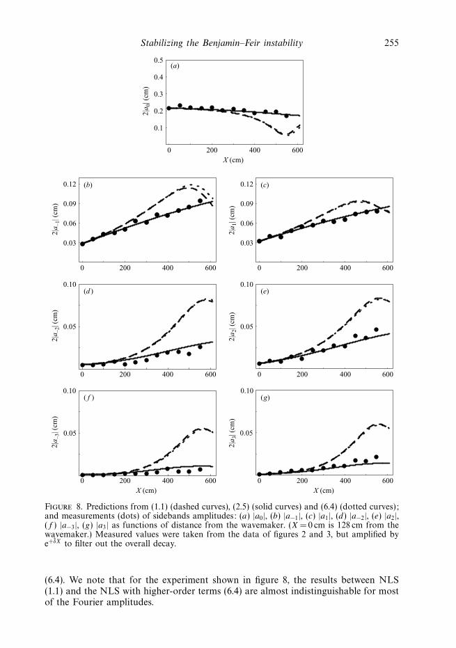
Figure 8. Predictions from (1.1) (dashed curves), (2.5) (solid curves) and (6.4) (dotted curves);and measurements (dots) of sidebands amplitudes: (a) |a0|, (b) |a−1|, (c) |a1|, (d) |a−2|, (e) |a2|,(f ) |a−3|, (g) |a3| as functions of distance from the wavemaker. (X = 0 cm is 128 cm from thewavemaker.) Measured values were taken from the data of figures 2 and 3, but amplified bye+δX to filter out the overall decay.
(6.4). We note that for the experiment shown in figure 8, the results between NLS(1.1) and the NLS with higher-order terms (6.4) are almost indistinguishable for mostof the Fourier amplitudes.
256 H. Segur and others
For this set of experiments, the damped NLS model, (2.1) in the form of(2.5), predicts the evolution of every measured amplitude much more accuratelythan either of the undamped models, (1.1) or (6.4). This striking discrepancy inaccuracy among these three mathematical models illustrates one of our main points.Equations (1.1) and (6.4) both predict that unstable sidebands stop growing aftertheir amplitudes become large enough that nonlinear interactions among sidebandsbecome dynamically important. Equation (2.1) provides another option: damping ofthe carrier wave can slow and eventually stop the growth of the unstable sidebandsaltogether, before their amplitudes become large enough that nonlinear interactionsplay a role. When this happens, sideband amplitudes always remain small, and thedifference between nonlinear terms in (1.1) and (6.4) has little effect on the evolutionof the wavetrain. Figure 8 demonstrates that this option occurs in the experimentsshown in figures 2 and 3: damping controls the growth of the sidebands, precludingserious nonlinear effects.
We are not suggesting that in the presence of damping, the processes described by(1.1) or (6.4) never occur. If the initial amplitudes of the seeded perturbations hadbeen larger, if the amplitude of the carrier wave had been larger, or if the dampingrate had been smaller, then nonlinear interactions among growing sidebands mighthave become important before damping effects took over. Instead, theorems 1 and 2assert that for fixed carrier-wave amplitude and fixed damping rate (so |γ ||A|2/δ isfixed in (4.8) or (4.19)), then a sideband perturbation that is small enough initiallymust remain small forever. In this way, a uniform train of plane waves of moderateamplitude in deep water is stable, for any δ > 0.
6.4. A second set of experiments
Figure 9 shows results from a second set of experiments, in which the seeded perturba-tion was chosen so that the B–F theory would predict instability even when the decayrate was subtracted from the growth rate, while the dissipative theory would predicta bound to growth that could be observed within the wave tank. For this experiment,ω0/2π = 3.33 Hz, ωp/2π = 0.39Hz and δ = 0.115 m−1. The time series shown in figures9(a) and 9(c) were obtained at X1 and X14, 650 cm apart. In this experiment there islittle evolution of the wavetrain other than that due to damping, because the sidebandsnever grow much. The Fourier amplitudes of the carrier wave and the two seededsidebands are shown in figures 9(e)–9(g). The dots are the measurements. The curvesshow computations from the linearized stability theory that includes damping, (4.3)(solid curves), and the NLS equation that includes higher-order terms, (6.4)–(dottedcurves). For both sets of curves, the starting values of the complex Fourier amplitudeswere:
2a0 = −0.014−0.229 i, 2a−1 = 0.012+0.001 i, 2a1 = −0.007+0.009 i, |an| = 0, |n| > 1.
As in figure 8, the data in figure 9 agree reasonably well with predictions fromthe stability theory for the uniform solution of (2.5), and agree less well withpredictions from (6.4). According to (2.1), damping essentially stops the sidebandgrowth, consistent with the observed behaviour. By contrast, this effect of damping isneglected by both (1.1) and (6.4), which predict continued growth of sidebands.
We reiterate: in the presence of damping, growth of an unstable sideband canstop either because of nonlinear interactions among sidebands, or because dampinghas quenched the growth of the sideband by decreasing the amplitude of the carrierwave (or both). For a fixed value of |γ ||A|2/δ, we can always guarantee that
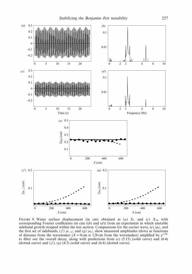
Stabilizing the Benjamin–Feir instability 257
0 5 10 15 20
0 5 10 15 20
0.1
0
0.2
–0.1
–0.2
0.3
0.1
0
0.2
–0.1
–0.2
0.3
(a) (b)
(c) (d )
0.01
0.1
0.01
0.1
0 2 3 86 10
0 2 3 86 10
( f ) (g)
0 200 400 600X (cm) X (cm)
0.1
0.2
2|a –
1| (
cm)
2|a 1
| (cm
)
0 200 400 600
0.1
0.2
(e)
0 200 400 600X (cm)
0.3
0.2
0.4
0.1
0.5
2|a 0
| (cm
)
Time (s) Frequency (Hz)
Figure 9. Water surface displacement (in cm) obtained at (a) X1 and (c) X14 withcorresponding Fourier coefficients (in cm) ((b) and (d)) from an experiment in which unstablesideband growth stopped within the test section. Comparisons for the carrier wave, (e) |a0|, andthe first set of sidebands, (f ) |a−1|, and (g) |a1|, show measured amplitudes (dots) as functionsof distance from the wavemaker (X = 0 cm is 128 cm from the wavemaker) amplified by e+δX
to filter out the overall decay, along with predictions from (e) (5.15) (solid curve) and (6.4)(dotted curve) and (f ), (g) (4.3) (solid curve) and (6.4) (dotted curve).
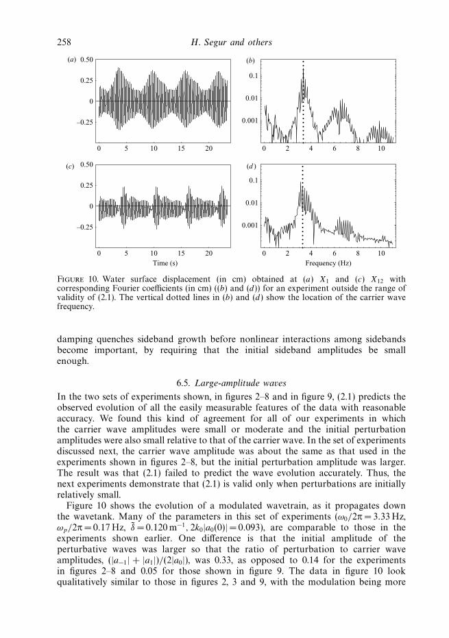
258 H. Segur and others
0 5 10 15 20
0.25
0
–0.25
0.50
0 5 10 15 20
0.25
0
–0.25
0.50
(a) (b)
(c) (d )
0.01
0.001
0.1
0.01
0.001
0.1
0 2 4 86 10
0 2 4 86 10Time (s) Frequency (Hz)
Figure 10. Water surface displacement (in cm) obtained at (a) X1 and (c) X12 withcorresponding Fourier coefficients (in cm) ((b) and (d)) for an experiment outside the range ofvalidity of (2.1). The vertical dotted lines in (b) and (d) show the location of the carrier wavefrequency.
damping quenches sideband growth before nonlinear interactions among sidebandsbecome important, by requiring that the initial sideband amplitudes be smallenough.
6.5. Large-amplitude waves
In the two sets of experiments shown, in figures 2–8 and in figure 9, (2.1) predicts theobserved evolution of all the easily measurable features of the data with reasonableaccuracy. We found this kind of agreement for all of our experiments in whichthe carrier wave amplitudes were small or moderate and the initial perturbationamplitudes were also small relative to that of the carrier wave. In the set of experimentsdiscussed next, the carrier wave amplitude was about the same as that used in theexperiments shown in figures 2–8, but the initial perturbation amplitude was larger.The result was that (2.1) failed to predict the wave evolution accurately. Thus, thenext experiments demonstrate that (2.1) is valid only when perturbations are initiallyrelatively small.
Figure 10 shows the evolution of a modulated wavetrain, as it propagates downthe wavetank. Many of the parameters in this set of experiments (ω0/2π = 3.33 Hz,ωp/2π = 0.17 Hz, δ = 0.120 m−1, 2k0|a0(0)| = 0.093), are comparable to those in theexperiments shown earlier. One difference is that the initial amplitude of theperturbative waves was larger so that the ratio of perturbation to carrier waveamplitudes, (|a−1| + |a1|)/(2|a0|), was 0.33, as opposed to 0.14 for the experimentsin figures 2–8 and 0.05 for those shown in figure 9. The data in figure 10 lookqualitatively similar to those in figures 2, 3 and 9, with the modulation being more
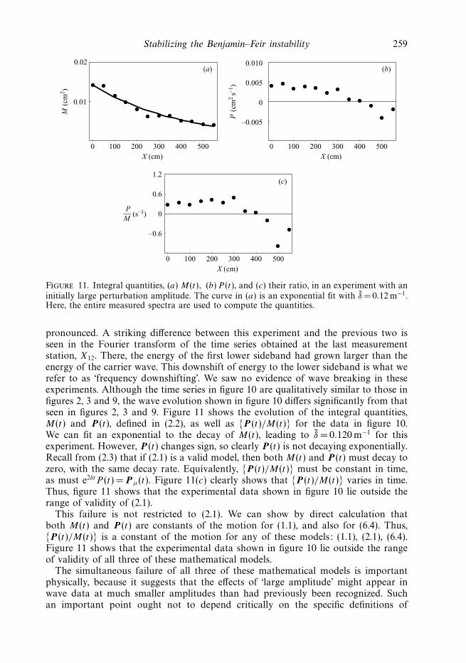
Stabilizing the Benjamin–Feir instability 259
0 100 200 300 400 500X (cm) X (cm)
0.01
0.02(a) (b)
M (
cm2 )
0 100 200 300 400 500
–0.005
0
0.005
0.010
0 100 200 300 400 500X (cm)
–0.6
0.6
0
1.2(c)
P (
cm2
s–1)
P— M
(s–1)
Figure 11. Integral quantities, (a) M(t), (b) P (t), and (c) their ratio, in an experiment with aninitially large perturbation amplitude. The curve in (a) is an exponential fit with δ = 0.12 m−1.Here, the entire measured spectra are used to compute the quantities.
pronounced. A striking difference between this experiment and the previous two isseen in the Fourier transform of the time series obtained at the last measurementstation, X12. There, the energy of the first lower sideband had grown larger than theenergy of the carrier wave. This downshift of energy to the lower sideband is what werefer to as ‘frequency downshifting’. We saw no evidence of wave breaking in theseexperiments. Although the time series in figure 10 are qualitatively similar to those infigures 2, 3 and 9, the wave evolution shown in figure 10 differs significantly from thatseen in figures 2, 3 and 9. Figure 11 shows the evolution of the integral quantities,M(t) and P(t), defined in (2.2), as well as P(t)/M(t) for the data in figure 10.We can fit an exponential to the decay of M(t), leading to δ = 0.120 m−1 for thisexperiment. However, P(t) changes sign, so clearly P(t) is not decaying exponentially.Recall from (2.3) that if (2.1) is a valid model, then both M(t) and P(t) must decay tozero, with the same decay rate. Equivalently, P(t)/M(t) must be constant in time,as must e2δtP (t) = Pµ(t). Figure 11(c) clearly shows that P(t)/M(t) varies in time.Thus, figure 11 shows that the experimental data shown in figure 10 lie outside therange of validity of (2.1).
This failure is not restricted to (2.1). We can show by direct calculation thatboth M(t) and P(t) are constants of the motion for (1.1), and also for (6.4). Thus,P(t)/M(t) is a constant of the motion for any of these models: (1.1), (2.1), (6.4).Figure 11 shows that the experimental data shown in figure 10 lie outside the rangeof validity of all three of these mathematical models.
The simultaneous failure of all three of these mathematical models is importantphysically, because it suggests that the effects of ‘large amplitude’ might appear inwave data at much smaller amplitudes than had previously been recognized. Suchan important point ought not to depend critically on the specific definitions of
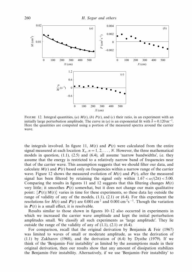
260 H. Segur and others
0 100 200 300 400 500X (cm) X (cm)
0.01
0.02(a) (b)
(c)
M (
cm2 )
0 100 200 300 400 500
–0.002
0
0.002
0.004
0 100 200 300 400 500X (cm)
–0.6
0.6
0
1.2
P (
cm2
s–1)
P— M
(s–1)
Figure 12. Integral quantities, (a) M(t), (b) P (t), and (c) their ratio, in an experiment with aninitially large perturbation amplitude. The curve in (a) is an exponential fit with δ = 0.120 m−1.Here the quantities are computed using a portion of the measured spectra around the carrierwave.
the integrals involved. In figure 11, M(t) and P(t) were calculated from the entiresignal measured at each location Xn, n = 1, 2, . . . , N . However, the three mathematicalmodels in question, (1.1), (2.5) and (6.4), all assume ‘narrow bandwidths’, i.e. theyassume that the energy is restricted to a relatively narrow band of frequencies nearthat of the carrier wave. This assumption suggests that we should filter our data, andcalculate M(t) and P(t) based only on frequencies within a narrow range of the carrierwave. Figure 12 shows the measured evolution of M(t) and P(t), after the measuredsignal has been filtered by retaining the signal only within 1.67 <ω/(2π) < 5.00.Comparing the results in figures 11 and 12 suggests that this filtering changes M(t)very little; it smoothes P(t) somewhat, but it does not change our main qualitativepoint: P(t)/M(t) varies in time for these experiments, so these data lay outside therange of validity of any of the models, (1.1), (2.1) or (6.4). For this experiment theresolutions for M(t) and P(t) are 0.001 cm 2 and 0.001 cm 2s −1. Though the variationin P(t) is a small effect, it is resolvable.
Results similar to those shown in figures 10–12 also occurred in experiments inwhich we increased the carrier wave amplitude and kept the initial perturbationamplitudes small. We classify all such experiments as ‘large amplitude’. They lieoutside the range of the validity of any of (1.1), (2.1) or (6.4).
For comparison, recall that the original derivation by Benjamin & Feir (1967)was limited to waves of small or moderate amplitude, as was the derivation of(1.1) by Zakharov (1968), and the derivation of (6.4) by Dysthe (1979). If wethink of the ‘Benjamin–Feir instability’ as limited by the assumptions made in theiroriginal derivation, then our results show that any amount of dissipation stabilizesthe Benjamin–Feir instability. Alternatively, if we use ‘Benjamin–Feir instability’ to
Stabilizing the Benjamin–Feir instability 261
describe events outside of the range stated in the original work of Benjamin & Feir,then the previous sentence is too strong.
6.6. What does ‘small or moderate amplitude’ mean?
The data shown in figures 2–9 demonstrate that the theory presented in this paperdescribes accurately the evolution of a nearly uniform train of nearly monochromaticwaves of small or moderate amplitude in deep water, provided the perturbations aresmall enough. The data in figures 10–12 show what can happen if either the amplitudeof the carrier wave is large enough, or if the perturbations are large enough. Forwaves with larger amplitudes, we have found experimentally that our theory losesaccuracy, and also that P(t)/M(t) decreases monotonically, as shown in figures 11(c)or 12(c). This ratio should be constant according to any of (1.1), (2.1) or (6.4), soits monotonic decrease indicates that all of these theories fail together. As far as wecan tell, the process that forces P(t)/M(t) to decrease is dissipative. If so, then anygeneralization of (1.1) or (6.4) that includes more terms in an asymptotic expansionwithin a non-dissipative model like Euler’s (conservative) equations will fail to capturethe physics of large-amplitude events.
What happens to waves of larger amplitude, which fall outside the range of validityof the theory presented here? This topic is worthy of a separate study, and we donot address it here. For this paper, we restrict our comments simply to defining whatwe mean by ‘moderate amplitude’ and ‘large amplitude’. Based on our experimentalresults, the critical issue seems to be whether P(t)/M(t) is conserved during theevolution. If P(t)/M(t) is conserved as the wavetrain evolves, then we classifythe wavetrain as having moderate amplitude and use (2.1). In our experiments,P(t)/M(t) was not conserved when using wavetrains with larger carrier waveamplitudes or larger perturbation amplitudes; in these experiments, (2.1) often failedto predict the evolution of more than one measured quantity.
We can state this criterion in various ways. Instead of monitoring P(t)/M(t), wecan use the evolution of M(t) to define δ for a particular set of experiments; thenthe wavetrain in those experiments has moderate amplitude if e2δt P(t) is constant (towithin experimental error) during the experiments. This is mathematically equivalentto monitoring Pµ(t), defined in (2.6).
A disadvantage of this criterion is that it is not predictive: we must run theexperiment and observe P(t)/M(t) in order to use the criterion. Two referees ofthis paper asked that we provide a simple a priori estimate to predict whether a givenwavetrain lies in the range of validity of the theory presented here.
This is an important question, but we are currently unable to give a completeanswer to it. Here is what we know.
(i) A common measure of nonlinearity for a nearly monochromatic train of wavesin deep water is the dimensionless slope of the wave, ε = 2k0|a0(0)|. (Recall that theextra factor of 2 arises because our crest-to-trough amplitude is 2|a0(0)|.)
(ii) The theory presented here fails for experiments that show wave-breaking,frequency downshifting or both; neither of these phenomena is predicted by (1.1), (2.1)or (6.4). Melville (1982) found experimentally that nearly monochromatic spatiallyuniform wavetrains showed signs of both wave-breaking and frequency downshiftingfor ε > 0.16.
(iii) Our experiments showed measurable changes in e2δt P(t) for ε > 0.14. This isconsistent with Melville’s observations.
(iv) The experiments in figure 10 show that frequency downshifting can occur evenfor wavetrains with ε < 0.14, if the perturbations are large enough.
262 H. Segur and others
(v) Finding an accurate, unambiguous criterion to determine which wavetrains are‘large’ enough to produce frequency downshifting or wave breaking is an importantopen question, in our minds.
When the model (2.1) is valid, the stability theory outlined in § 4 says that dissipationbounds the growth of sidebands before nonlinear interactions become important,provided the sidebands have a small enough initial amplitude. Here are two thoughtsconcerning the application of this theory.
(i) A bound on growth due to dissipation is given by (4.5) to be e|γ |M/δ . Anapproximate WKB analysis of (4.3), which we do not outline here, suggests that thetotal growth is more likely to be about e|γ |M/3δ when M/δ is large. In the experimentspresented herein, dissipation bounded the growth of sidebands before nonlinearinteractions became important. We do not have a bound above which nonlinearinteractions become important, but no downshifting occurs.
(ii) For the experiments discussed herein, the initial data had a narrow bandwidthand dissipation kept the bandwidth narrow, so that the higher-order model (6.4)that includes broader bandwidth effects, but not dissipation, did not apply. If thedata initially had a broader bandwidth, then a higher-order model might be moreappropriate, but our results indicate that modifying (6.4) to include dissipation islikely to be necessary.
7. Comparison with earlier experimental resultsOur main result is that even a small amount of dissipation controls the Benjamin–
Feir instability for nearly monochromatic waves of moderate amplitude in deep water.However, this instability is well established in water waves, in optics and elsewhere.In this section, we re-examine some of the earlier experimental work that is cited insupport of the B–F instability.
In the literature on waves in deep water, two kinds of experiment have been donethat relate to the Benjamin–Feir instability. Experiments by Feir (1967), Yuen & Lake(1975), Su (1982), and Trulsen & Stansberg (2001) focused on the evolution of spatiallylocalized wave packets, and these do not concern us here. Instead, we concentrate onexperiments that involve modulations of a continuous train of nearly monochromaticwaves, because they are consistent with the periodic boundary conditions used in thispaper. Specifically, we now reconsider the experiments described by Benjamin (1967),Lake et al. (1977), Lake & Yuen (1977) and Melville (1982) on waves in deep water,and by Tai et al. (1986) on electromagnetic waves in an optical fibre. In all of theseexperiments, the observed waves were essentially one-dimensional, corresponding toβ = 0 or ∂y ≡ 0 in (1.1) or (2.1).
In our reading of these papers, all of the experimental studies designed to test theBenjamin–Feir mechanism found discrepancies between the non-dissipative theoryand physical experiments. Benjamin (1967) described preliminary experimental results,which provided qualitative support for the new theory of Benjamin & Feir (1967).Those experiments showed:
(i) energy grows in sideband frequencies, at the expense of the carrier wave;(ii) the range of unstable sideband frequencies is set by the amplitude of the
carrier wave (as shown in (4.4), with β = 0 for one-dimensional waves and δ = 0 forno dissipation);
(iii) no actual, physical growth occurs unless the inviscid growth rate exceeds theviscous damping rate.
Stabilizing the Benjamin–Feir instability 263
All of these results are consistent with (2.1). It is not necessary to conclude fromthem that there is an instability, as defined by (2.10) and (2.11).
In his figure 4, Benjamin (1967) compared measured growth rates with valuespredicted by the inviscid theory, with a correction for viscous decay. (His correctionwas: observed growth rate = predicted growth rate – viscous decay rate. Ourprocedure of amplifying the measured data by eδt is nearly equivalent to his.) Hispresentation of the data inherently assumes that any sideband growth is exponential,so it precludes the kind of varying growth shown in our figure 5. He found thatobserved growth rates are consistently smaller than those predicted by the Benjamin–Feir theory, even after correcting for damping, with discrepancies ranging from 40 %to 100 %. As our figures 5, 6, 8, 9 show, actual growth rates decrease with ‘time’ (i.e.as the wave propagates down the tank). Benjamin’s correction gives a growth ratethat is correct for short times, but too large for longer times.
Thus, the ground-breaking experiments reported by Benjamin (1967) show clearlythat energy in sidebands can grow at the expense of the carrier wave, but they do notactually establish an instability. Further, they show that the Benjamin–Feir theoryover-predicts the observed growth rate, even with a correction for damping. All ofthis is consistent with (2.1).
Benjamin (1967) reports a measured damping rate of 0.01/wavelength in hisexperiments. In Benjamin’s notation, our measured damping rate is 0.016/wavelength[ = δ(2π/k0)] for the experiments shown in figures 2–8. Thus, our damping rate wascomparable to Benjamin’s. None of the other experimental papers on waves in deepwater (Feir 1967; Lake & Yuen 1977; Lake et al. 1977; Melville 1982; Su 1982; Tulin &Waseda 1999; Trulsen & Stansberg 2001) reported measured damping rates.
The discrepancies shown by Benjamin (1967) inspired Lake, Yuen, and theircolleagues to conduct a second set of experiments to test the Benjamin–Feir theory.Lake & Yuen (1977) reported that in their experiments, the carrier wave and its secondharmonic did not satisfy our (3.2). They attributed this difficulty to problems withtheir paddle, which could be consistent with the problems with paddle motion citedby Flick & Guza (1980). However, in a later paper Lake & Yuen state, ‘this effect isfar less significant than was believed and should be disregarded’ (See Crawford et al.1981, p. 184). Regardless of their reasoning, our figure 7(b) shows that our data dosatisfy (3.2), so their problems with (3.2) are not inherent in deep-water waves.
Based on our own experiments, we wonder if some of their problems with (3.2)can be attributed to reflected waves in their tank. (See Lake et al. 1977, p. 52: ‘Eachexperimental condition or run was recorded for at least 12 min of real time.’ Theirtank was 40 ft long, so a deep-water wave with a frequency of 3 Hz travels at its owngroup velocity down the tank and back in about 94 s, much shorter than 12 min.) Forcomparison, our experiments ran for much shorter time intervals, and our figure 7(b)shows good agreement with (3.2). In an experiment run for their long times, the tankprobably contains waves running both upstream and downstream. A probe at a fixedlocation cannot determine the direction of propagation of a wave passing the probe,but only waves moving downstream should be included in (3.2).
A major conclusion of Lake & Yuen (1977) was that the one-dimensional wavemode with the maximal growth rate did not satisfy our (3.7b) with l = 0, as predictedby the Benjamin–Feir theory. Translating their result into our notation, they foundthat the most unstable mode satisfied
m = 0.78
√γ
α|A|, instead of m =
√γ
α|A|
264 H. Segur and others
as predicted by (3.7b). This finding is consistent with (2.1), because the mode that ismost unstable at t = 0 ceases to be most unstable for t > 0. As a result, modes withwavenumbers smaller than m =
√γ /α|A| can show more total growth over the length
of the test section, and this is what Lake & Yuen (1977) observed.A second major conclusion of Lake & Yuen (1977, p. 56) is that ‘. . . the data show
that the exponential rate of sideband growth remains essentially constant, indicatingthat the second-order effect of dissipation is also unimportant during the initial stageof evolution . . . ’ This claim is consistent with our figure 5 for about the first 2 m ofpropagation in our experiments, but it contradicts our results for the remaining 4 m.In order to create a longer ‘effective’ test section, Lake & Yuen spliced togetherresults from several experiments in creating their figure 3. As far as we can tell, theirsplicing procedure did not allow the carrier wave to decay as it would have in a singleexperiment. We wonder about the validity of their splicing procedure. Certainly ourresults contradict theirs, except for short distances.
Melville (1982) studied the relation between the B–F instability and wave breakingin deep water. As mentioned above, the original analysis of Benjamin & Feir (1967)was restricted to waves of moderate amplitude, so Melville’s definition of ‘B–Finstability’ is generalized from that originally discussed by Benjamin & Feir to includewaves of large amplitude. Melville’s carrier wave amplitudes were much larger thanthose considered here, which led him to conclude that his experiments were outsidethe range of validity of (1.1). There seems to be little overlap between his experimentalregime and ours: our results apply to waves of small and moderate amplitude, whilehe considered primarily waves of large amplitude. Tulin & Waseda (1999) were alsointerested in breaking waves, and considered primarily waves of large amplitude.
Finally, Tai et al. (1986) described their experiments on modulational (i.e. B–F)instabilities of electromagnetic waves in an optical fibre. Like the earlier experimentsof Benjamin (1967), their experiments show that sidebands can gain energy at theexpense of the carrier wave, but it is impossible to tell from their data whether thisgrowth is exponential, or variable (as predicted by (2.1)). No actual growth rates arepresented. Like Lake & Yuen (1977), they found that the frequency-difference betweenthe carrier wave and the most unstable sideband mode increased as the carrier waveamplitude increased, but the increase was slower than that predicted by (3.6b). All ofthis is consistent with (2.1) instead of (1.1), so it is consistent with a conclusion ofsideband growth, but no actual instability.
In summary, all of the studies known to us that compare the predictions ofBenjamin & Feir (1967) with experimental data show that energy in sidebands cangrow at the expense of the carrier wave, and our experiments show this as well. Wefound no experimental studies showing that the growth is actually exponential, insteadof the variable growth predicted by (2.1). Similarly, we found no experimental studiesshowing that the growth is part of an actual instability in the sense of (2.10) and(2.11). Our own experiments, discussed in § 6, show that the growth is not exponential,and that there is no actual instability for waves of moderate amplitude.
We are grateful to Bernard Deconinck for useful conversations, and to GuillemetteCaulliez for suggesting the experiment shown in figure 9. We dedicate this paperto the memory Joe Hammack, who passed away during its publication, and tothe memory of Bill Pritchard, who built the wave tank used herein with the ideaof revisiting the Benjamin–Feir instability. This work was funded in part by theNational Science Foundation, under grants DMS-9972210, DMS-0139771, DMS-0139742, DMS-0139847, and by Packard and Sloan Fellowships.
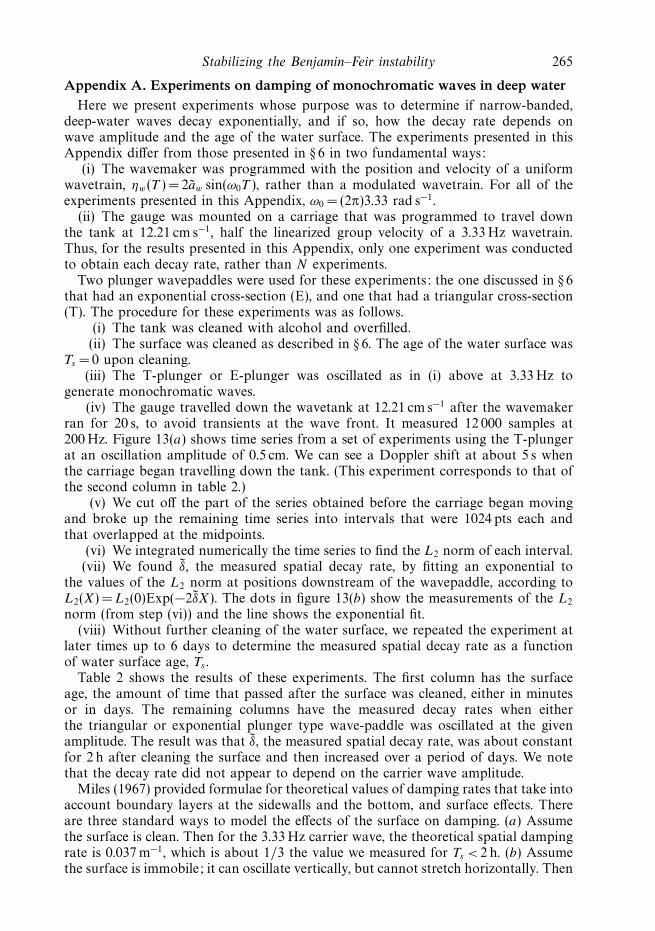
Stabilizing the Benjamin–Feir instability 265
Appendix A. Experiments on damping of monochromatic waves in deep waterHere we present experiments whose purpose was to determine if narrow-banded,
deep-water waves decay exponentially, and if so, how the decay rate depends onwave amplitude and the age of the water surface. The experiments presented in thisAppendix differ from those presented in § 6 in two fundamental ways:
(i) The wavemaker was programmed with the position and velocity of a uniformwavetrain, ηw(T ) = 2aw sin(ω0T ), rather than a modulated wavetrain. For all of theexperiments presented in this Appendix, ω0 = (2π)3.33 rad s−1.
(ii) The gauge was mounted on a carriage that was programmed to travel downthe tank at 12.21 cm s−1, half the linearized group velocity of a 3.33 Hz wavetrain.Thus, for the results presented in this Appendix, only one experiment was conductedto obtain each decay rate, rather than N experiments.
Two plunger wavepaddles were used for these experiments: the one discussed in § 6that had an exponential cross-section (E), and one that had a triangular cross-section(T). The procedure for these experiments was as follows.
(i) The tank was cleaned with alcohol and overfilled.(ii) The surface was cleaned as described in § 6. The age of the water surface was
Ts = 0 upon cleaning.(iii) The T-plunger or E-plunger was oscillated as in (i) above at 3.33 Hz to
generate monochromatic waves.(iv) The gauge travelled down the wavetank at 12.21 cm s−1 after the wavemaker
ran for 20 s, to avoid transients at the wave front. It measured 12 000 samples at200 Hz. Figure 13(a) shows time series from a set of experiments using the T-plungerat an oscillation amplitude of 0.5 cm. We can see a Doppler shift at about 5 s whenthe carriage began travelling down the tank. (This experiment corresponds to that ofthe second column in table 2.)
(v) We cut off the part of the series obtained before the carriage began movingand broke up the remaining time series into intervals that were 1024 pts each andthat overlapped at the midpoints.
(vi) We integrated numerically the time series to find the L2 norm of each interval.(vii) We found δ, the measured spatial decay rate, by fitting an exponential to
the values of the L2 norm at positions downstream of the wavepaddle, according toL2(X) = L2(0)Exp(−2δX). The dots in figure 13(b) show the measurements of the L2
norm (from step (vi)) and the line shows the exponential fit.(viii) Without further cleaning of the water surface, we repeated the experiment at
later times up to 6 days to determine the measured spatial decay rate as a functionof water surface age, Ts .
Table 2 shows the results of these experiments. The first column has the surfaceage, the amount of time that passed after the surface was cleaned, either in minutesor in days. The remaining columns have the measured decay rates when eitherthe triangular or exponential plunger type wave-paddle was oscillated at the givenamplitude. The result was that δ, the measured spatial decay rate, was about constantfor 2 h after cleaning the surface and then increased over a period of days. We notethat the decay rate did not appear to depend on the carrier wave amplitude.
Miles (1967) provided formulae for theoretical values of damping rates that take intoaccount boundary layers at the sidewalls and the bottom, and surface effects. Thereare three standard ways to model the effects of the surface on damping. (a) Assumethe surface is clean. Then for the 3.33 Hz carrier wave, the theoretical spatial dampingrate is 0.037 m−1, which is about 1/3 the value we measured for Ts < 2 h. (b) Assumethe surface is immobile; it can oscillate vertically, but cannot stretch horizontally. Then
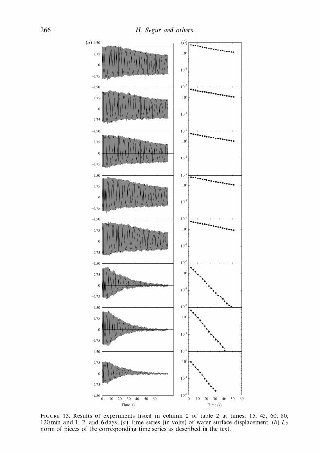
266 H. Segur and others
–1.50
–0.75
0
0.75
1.50(a) (b)
10–2
10–1
100
–1.50
–0.75
0
0.75
10–2
10–1
100
–1.50
–0.75
0
0.75
10–2
10–1
100
–1.50
–0.75
0
0.75
10–2
10–1
100
–1.50
–0.75
0
0.75
10–2
10–1
100
–1.50
–0.75
0
0.75
10–2
10–1
100
–1.50
–0.75
0
0.75
10–2
10–1
100
–1.50
–0.75
0
0.75
10–2
10–1
100
0 10 20 30 40 50 60 0 10 20 30 40 50 60
Time (s) Time (s)
Figure 13. Results of experiments listed in column 2 of table 2 at times: 15, 45, 60, 80,120min and 1, 2, and 6 days. (a) Time series (in volts) of water surface displacement. (b) L2
norm of pieces of the corresponding time series as described in the text.
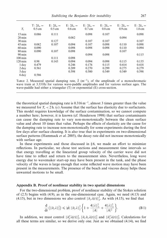
Stabilizing the Benjamin–Feir instability 267
T: 2aw = E: 2aw = E: 2aw = E: 2aw = E: 2aw = E: 2aw = E: 2aw =Ts 0.5 cm 0.5 cm 0.6 cm 0.7 cm 0.8 cm 0.9 cm 1.0 cm
15min 0.086 0.111 0.098 0.107 0.09820min 0.082 0.09430min 0.127 0.107 0.107 0.10745min 0.082 0.107 0.094 0.107 0.098 0.110 0.09860min 0.090 0.098 0.098 0.098 0.110 0.09480min 0.090 0.107 0.098 0.10790min 0.094 0.098 0.115
100 min 0.111 0.098120 min 0.98 0.143 0.094 0.094 0.098 0.115 0.135
1 day 0.479 0.246 0.176 0.115 0.414 0.4182 day 0.561 0.209 0.270 0.299 0.275 0.2795 day 0.598 0.500 0.549 0.549 0.5986 day 0.586
Table 2. Measured spatial damping rate, δ (m−1), of the amplitude of a monochromaticwave train at 3.33 Hz for various wave-paddle amplitudes and for various surface ages. Thewave-paddle had either a triangular (T) or exponential (E) cross-section.
the theoretical spatial damping rate is 0.316 m−1, almost 3 times greater than the valuewe measured for Ts < 2 h. (c) Assume that the surface has elasticity due to surfactants.This model requires knowledge of the surface contamination, so we cannot computea number here; however, it is known (cf. Henderson 1998) that surface contaminantscan cause the damping rate to vary non-monotonically between the clean surfacevalue and about 10 times that value. Perhaps the effects of elasticity are the cause forthe damping rate to increase non-monotonically for some experiments during the firstfew days after surface cleaning. It is also true that in experiments on two-dimensionalsurface patterns (Hammack et al. 2005), the decay rate did not increase monotonicallywith surface age.
In these experiments and those discussed in § 6, we made an effort to minimizereflections. In particular, we chose test sections and measurement time intervals sothat energy travelling at the linearized group velocity of the carrier wave did nothave time to reflect and return to the measurement sites. Nevertheless, long waveenergy due to wavemaker start-up may have been present in the tank, and the phasevelocity of the waves is large enough that some reflected wave motion may have beenpresent in the measurements. The presence of the beach and viscous decay helps theseunwanted motions to be small.
Appendix B. Proof of nonlinear stability in two spatial dimensionsFor the two-dimensional problem, proof of nonlinear stability of the Stokes solution
of (2.5) begins with (4.9), as in the one-dimensional case. Again, we need (4.13) and(4.15), but in two dimensions we also control ‖∂yλ(t)‖2
2. As with (4.15), we find that
d
dt
(‖∂yλ‖2
2
) |φ| ‖∂yλ‖2
2
1 +
4‖λ‖2∞
|A| +4‖λ‖2
∞|A|2
. (B 1)
In addition, we must control ‖∂2xλ(t)‖2
2, ‖∂x∂yλ(t)‖22 and ‖∂2
yλ(t)‖22. Calculations for
all these terms are similar, so we derive only one. Just as we obtained (4.14), we find
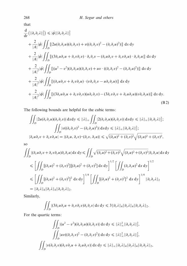
268 H. Segur and others
that
d
dt
(‖∂x∂yλ‖2
2
) |φ|‖∂x∂yλ‖2
2
+2
|A| |φ|∫∫
D
[|2u(∂x∂yu)(∂x∂yv) + v((∂x∂yv)2 − (∂x∂yu)2)|] dx dy
+2
|A| |φ|∫∫
D
[|(3∂xu∂yu + ∂xv∂yv) · ∂x∂yv − (∂xu∂yv + ∂xv∂yu) · ∂x∂yu|] dx dy
+2
|A|2|φ|
∫∫D
[|(u2 − v2)(∂x∂yu)(∂x∂yv) + uv · ((∂x∂yv)2 − (∂x∂yu)2)|] dx dy
+2
|A|2|φ|
∫∫D
[|(∂xu∂yv + ∂xv∂yu) · (v∂x∂yv − u∂x∂yu)|] dx dy
+2
|A|2|φ|
∫∫D
[|(3∂xu∂yu + ∂xv∂yv)(u∂x∂yv) − (3∂xv∂yv + ∂xu∂yu)(v∂x∂yu)|] dx dy.
(B 2)
The following bounds are helpful for the cubic terms:∫∫D
|2u(∂x∂yu)(∂x∂yv)| dxdy ‖λ‖∞
∫∫D
|2(∂x∂yu)(∂x∂yv)| dxdy ‖λ‖∞‖∂x∂yλ‖22;∫∫
D
|v((∂x∂yv)2 − (∂x∂yu)2)| dxdy ‖λ‖∞‖∂x∂yλ‖22;
|∂xu∂yv + ∂xv∂yu| = |(∂xu, ∂xv) · (∂yv, ∂yu)| √
(∂xu)2 + (∂xv)2√
(∂yu)2 + (∂yv)2,
so∫∫D
|(∂xu∂yv + ∂xv∂yu)∂x∂yu|dx dy
∫∫D
√(∂xu)2 +(∂xv)2
√(∂yu)2 +(∂yv)2|∂x∂yu|dx dy
[∫∫D
[(∂xu)2 + (∂xv)2][(∂yu)2 + (∂yv)2] dx dy
]1/2 [∫∫D
(∂x∂yu)2 dx dy
]1/2
[∫∫D
[(∂xu)2 + (∂xv)2]2 dx dy
]1/4 [∫∫D
[(∂yu)2 + (∂yv)2]2 dx dy
]1/4
‖∂x∂yλ‖2
= ‖∂xλ‖4‖∂yλ‖4‖∂x∂yλ‖2.
Similarly, ∫∫D
|(3∂xu∂yu + ∂xv∂yv)∂x∂yv| dx dy 3‖∂xλ‖4‖∂yλ‖4‖∂x∂yλ‖2.
For the quartic terms:∫∫D
|(u2 − v2)(∂x∂yu)(∂x∂yv)| dx dy ‖λ‖2∞‖∂x∂yλ‖2
2,∫∫D
|uv((∂x∂yv)2 − (∂x∂yv)2)| dx dy ‖λ‖2∞‖∂x∂yλ‖2
2,∫∫D
|v(∂x∂yv)(∂xv∂yu + ∂xu∂yv)| dx dy ‖λ‖∞‖∂xλ‖4‖∂yλ‖4‖∂x∂yλ‖2,
Stabilizing the Benjamin–Feir instability 269∫∫D
|u(∂x∂yu)(∂xv∂yu + ∂xu∂yv)| dx dy ‖λ‖∞‖∂xλ‖4‖∂yλ‖4‖∂x∂yλ‖2,∫∫D
|u(∂x∂yv)(3∂xu∂yv + ∂xv∂yu)| dx dy 3‖λ‖∞‖∂xλ‖4‖∂yλ‖4‖∂x∂yλ‖2,∫∫D
|v(∂x∂yu)(3∂xv∂yv + ∂xu∂yu)| dx dy 3‖λ‖∞‖∂xλ‖4‖∂yλ‖4‖∂x∂yλ‖2.
Using these bounds in (B 2) and regrouping leads to
d
dt
(‖∂x∂yλ‖2
2
) |φ|‖∂x∂yλ‖2
2
[1 +
2‖λ‖∞
|A|
]2
+ |φ|‖∂x∂yλ‖2
[1 +
2‖λ‖∞
|A|
](8‖∂xλ‖4‖∂yλ‖4
|A|
). (B 3)
In this same way, we also obtain
d
dt
(∥∥∂2xλ
∥∥2
2
) |φ|
∥∥∂2xλ
∥∥2
2
[1 +
2‖λ‖∞
|A|
]2
+ |φ|∥∥∂2
xλ∥∥
2
[1 +
2‖λ‖∞
|A|
](8‖∂xλ‖2
4
|A|
),
and
d
dt
(∥∥∂2yλ
∥∥2
2
) |φ|
∥∥∂2yλ
∥∥2
2
[1 +
2‖λ‖∞
|A|
]2
+ |φ|∥∥∂2
yλ∥∥
2
[1 +
2‖λ‖∞
|A|
](8‖∂yλ‖2
4
|A|
).
Adding these yields
d
dt
(∥∥∂2xλ
∥∥2
2+ ‖∂x∂yλ‖2
2 +∥∥∂2
yλ∥∥2
2
) |φ|
(∥∥∂2xλ
∥∥2
2+ ‖∂x∂yλ‖2
2 +∥∥∂2
yλ∥∥2
2
)[1 +
2‖λ‖∞
|A|
]2
+8
|A| |φ|[1 +
2‖λ‖∞
|A|
](∥∥∂2xλ
∥∥2‖∂xλ‖2
4 + ‖∂x∂yλ‖2‖∂xλ‖4‖∂yλ‖4 +∥∥∂2
yλ∥∥
2‖∂yλ‖2
4
). (B 4)
Now we define a Sobolev norm different from that in (4.16):
‖λ‖22,2 = ‖λ‖2
2 + ‖∂xλ‖22 + ‖∂yλ‖2
2 + ‖∂2xλ‖2
2 + ‖∂x∂yλ‖22 + ‖∂2
yλ‖22. (B 5)
Then we invoke more Sobolev inequalities (Adams 1975, p. 97). In two spatialdimensions:
(i) there is a positive constant C2, independent of λ, such that
‖λ‖∞ C2‖λ‖2,2; (B 6)
(ii) there is a positive constant C3, independent of λ, such that
‖∂xλ‖4 C3
[‖∂xλ‖2
2 +∥∥∂2
xλ∥∥2
2+ ‖∂x∂yλ‖2
2
]1/2, (B 7)
and
‖∂yλ‖4 C3
[‖∂yλ‖2
2 + ‖∂x∂yλ‖22 +
∥∥∂2yλ
∥∥2
2
]1/2.
Now combine (4.13), (4.15), (B 1) and (B 5), make use of (B 6) and (B 7), to obtain
d
dt
(‖λ‖2
2,2
) |φ|‖λ‖2
2,2
[1 +
2C2‖λ‖2,2
|A|
]2
+ |φ|‖λ‖22,2
[1 +
2C2‖λ‖2,2
|A|
](24C2
3
‖λ‖2,2
|A|
).
(B 8)
270 H. Segur and others
Hence, if there is a constant K , such that ‖λ(t)‖2,2 K < ∞ for all t 0, then itfollows from (B 8) and Gronwall’s inequality that
‖λ(t)‖22,2 ‖λ(0)‖2
2,2 exp
|φ(t)
[1 +
2C2K
|A|
][1 +
(2C2 + 24C2
3
)K
|A|
]. (B 9)
Thus, for all t 0,
‖λ(t)‖22,2 < ε,
provided at t = 0,
‖λ(0)‖21,2 < ∆ ε exp
− |γ ||A|2
δ
(1 +
2C2
√ε
|A|
)[1 +
(2C2 + 24C2
3
)√ε
|A|
], (B 10)
where we have chosen K √
ε. This completes the proof of theorem 2 in twodimensions: the Stokes solutions of (2.5) and of (2.1) are nonlinearly stable to smallperturbations in either one or two dimensions.
REFERENCES
Ablowitz, M. J. & Segur, H. 1981 Solitons and the Inverse Scattering Transform. SIAM,Philadelphia, 391 pp.
Adams, R. A. 1975 Sobolev Spaces. Academic, 259 pp.
Anderson, D. & Lisak, M. 1984 Modulational instability of coherent optical-fibre transmissionsignals. Opt. Lett. 9, 468–470.
Benjamin, T. B. 1967 Instability of periodic wavetrains in nonlinear dispersive systems. Proc. R.Soc. A 299, 59–75.
Benjamin, T. B. & Feir, J. E. 1967 The disintegration of wavetrains in deep water. Part 1. J. FluidMech. 27, 417–430.
Benney, D. J. & Newell, A. C. 1967 The propagation of nonlinear wave envelopes. Stud. Appl.Maths 46, 133–139.
Cherry, T. M. 1926 On periodic solutions of Hamiltonian systems of differential equations. Phil.Trans. R. Soc. Lond. A 227, 137–221.
Coddington, E. A. & Levinson, N. 1955 Theory of Ordinary Differential Equations. McGraw-Hill,429 pp.
Crawford, D. R., Lake, B. M., Saffman, P. G. & Yuen, H. C. 1981 Stability of deep-water wavesin two and three dimensions. J. Fluid Mech. 105, 177–191.
Dysthe, K. 1979 Note on a modification to the nonlinear Schrodinger equation for application todeep water waves. Proc. R. Soc. A 369, 105–114.
Feir, J. E. 1967 Discussion: some results from wave pulse experiments. Proc. R. Soc. A 299, 54–58.
Flick, R. E. & Guza, R. T. 1980 Paddle generated waves in laboratory channels. J. Waterway PortCosatal Ocean Div. WW1 ASCE 106, 79–97.
Gordon, J. P. 1986 Theory of the soliton self-frequency shift. Optics Lett. 11, 662–664.
Guenther, R. B. & Lee, J. W. 1988 Partial Differential Equations of Mathematical Physics andIntegral Equations. Dover, 557 pp.
Hammack, J. L. & Henderson, D. M. 2003 Experiments on deep-water waves with two-dimensionalsurface patterns. J. Offshore Mech. Arctic Engng 125, 48–53.
Hammack, J. L. Henderson, D. M. & Segur, H. 2005 Progressive waves with persistent two-dimensional surface patterns in deep water. J. Fluid Mech. 532, 1–51.
Hasegawa, A. 1971 Theory and computer experiment on self-trapping instability of plasma cyclotronwaves. Phys. Fluids 15, 870–881.
Hasegawa, A. & Kodama, Y. 1995 Solitons in Optical Communications. Clarendon, 320 pp.
Henderson, D. M. 1998 Effects of surfactants on Faraday wave dynamics. J. Fluid Mech. 365,89–107.
Ince, E. L. 1956 Ordinary Differential Equations. Dover, 558 pp.
Karlsson, M. 1995 Modulational instability in lossy optical fibers. J. Opt. Soc. Am. B 12, 2071–2077.
Stabilizing the Benjamin–Feir instability 271
Lake, B. M. & Yuen, H. C. 1977 A note on some water-wave experiments and the comparison ofdata with theory. J. Fluid Mech. 83, 75–81.
Lake, B. M., Yuen, H. C., Rungaldier, H. & Ferguson, W. E. 1977 Nonlinear deep-water waves:theory and experiment. Part 2. Evolution of a continuous wave train. J. Fluid Mech. 83, 49–74.
Lighthill, M. J. 1965 Contribution to the theory of waves in nonlinear dispersive systems. J. Inst.Math. Applics. 1, 269–306.
Lo, E. & Mei, C. C. 1985 A numerical study of water-wave modulations based on a higher-ordernonlinear Schrodinger equation. J. Fluid Mech. 150, 395–416.
Luther, G. G. & McKinstrie, C. J. 1990 Transverse modulational instability of collinear waves.J Opt. Soc. Am. B 7, 1125–1141.
McKinstrie, C. J. & Bingham, R. 1989 The modulational instability of coupled waves. Phys. FluidsB 1, 230–237.
Mei, C. C. & Hancock, M. J. 2003 Weakly nonlinear surface waves over a random seabed. J. FluidMech. 475, 247–268.
Melville, W. K. 1982 The instability and breaking of deep-water waves. J. Fluid Mech. 115, 65–185.
Miles, J. W. 1967 Surface-wave damping in closed basins. Proc. R. Soc. A 297, 459–475.
Nemytskii, V. V. & Stepanov, V. V. 1960 Qualitative Theory of Differential Equations. PrincetonUniversity Press, 519 pp.
Ostrovsky, L. A. 1967 Propagation of wave packets and space-time self-focussing in a nonlinearmedium. Sov. Phys. J. Exp. Theor. Phys. 24, 797–800.
Stokes, G. G. 1847 On the theory of oscillatory waves. Trans. Camb. Phil. Soc. 8, 441. Also inMathematical and Physical Papers, vol. 1, pp. 197–229.
Su, Y.-M. 1982 Evolution of groups of gravity waves with moderate to high steepness. Phys. Fluids25, 2167–2174.
Sulem, C. & Sulem, P. L. 1999 The Nonlinear Schrodinger Equation, Springer, 345 pp.
Tai, K., Tomita, A. & Hasegawa, A. 1986 Observation of modulational instability in optical fibres.Phys. Rev. Lett. 56, 135–138.
Tulin, M. P. & Waseda, T. 1999 Laboratory observations of wave group evolution, includingbreaking effects. J. Fluid Mech. 378, 197–232.
Trulsen, K., Kliakhandler, I., Dysthe, K. B. & Velarde, M. G. 2000 On weakly nonlinearmodulations of waves in deep water. Phys. Fluids, 12, 2432–2437.
Trulsen, K. & Stansberg, C. T. 2001 Spatial evolution of water surface waves. Proc. Eleventh IntlOffshore & Polar Engng Conf. pp. 71–77.
Whitham, G. B. 1967 Nonlinear dispersion of water waves. J. Fluid Mech. 27, 399–412.
Yuen, H. C. & Lake, B. M. 1975 Nonlinear deep water waves: theory and experiment Phys. Fluids18, 956–960.
Zakharov, V. E. 1967 Instability of self-focusing of light. Sov. Phys. J. Exp. Theor. Phys. 24, 455–459.
Zakharov, V. E. 1968 Stability of periodic waves of finite amplitude on the surface of a deep fluid.J. Appl. Mech. Tech. Phys. 2, 190–194.