Directions for using AnalysisTemplatev3

Directions for using AnalysisTemplatev3

From this Web site, you can download two types of Excel files:

1. River Data files

2. An Analysis Template

There is a single Excel workbook for each of 11 river stations that are included in our

monitoring program. Each workbook contains data for the period of record for that station.

These files are read-only files, as downloaded from the Download Page. Once they are

downloaded, they may be copied and modified. To assure that the files have not been

inappropriately modified by users and to receive data updates as they become available,.

we request that individual users download these files from our Web site rather than received

them from other users.

The AnalysisTemplatev3 is an Excel 2003 Workbook that will help you analyze the data in

the River Data files. This template contains macros that were developed to be compatible

with Office 2003. Therefore, if you are using Office 2007 software, this version of the

Analysis Template will NOT operate correctly, so please use AnalysisTemplatev4 which has

been developed to be compatible with Office 2007. In order to download and operate this

program, you must set the Macro Security to medium level and click Enable Macros when

your computer asks whether or not to open the file.

To set the Excel macro security level to medium, open an Excel workbook, under the Tool

menu, select Options. Under the Options menu, select Security, and under Security select

Macro Security. Set the Macro Security at Medium.

The Macros in this program are protected. For information on the Macros, contact the

Project Director (David Baker at [email protected]).

1. Download the Excel River Data

files and the

AnalysisTemplatev3 file to your

own computer and place them in

a single folder. See the

Download Page. You may

download as many of river data

files as you would like.

2. Do not change the names of any

of the files. These specific river

file names and the

AnalysisTemplatev3 file name

are referred to in the macros.

Alteration of the names will

cause the analysis program to

fail.

3. Do not open the

AnalysisTemplatev3 file by

double clicking it in the folder. If

you do, you may be prompted to

open each river file that you

choose to analyze. Instead,

open any other Excel file first,

then, under the File menu at the

top of the page, select Open and

navigate to the folder containing

the river data files and

AnalysisTemplatev3 file. You

may then double click on the

AnalysisTemplatev3 file. If you

open it this way, it will

automatically open any river files

it needs that are available in that

folder.

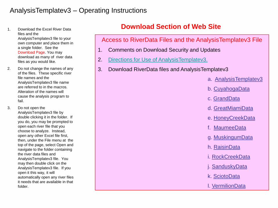
AnalysisTemplatev3 – Operating Instructions

Access to RiverData Files and the AnalysisTemplatev3 File

1. Comments on Download Security and Updates

2. Directions for Use of AnalysisTemplatev3.

3. Download RiverData files and AnalysisTemplatev3

a. AnalysisTemplatev3

b. CuyahogaData

c. GrandData

d. GreatMiamiData

e. HoneyCreekData

f. MaumeeData

g. MuskingumData

h. RaisinData

i. RockCreekData

j. SanduskyData

k. SciotoData

l. VermilionData

Download Section of Web Site

http://wql-data.heidelberg.edu/DirectionsAnalysisTemplate.pdf

1. When you open the AnalysisTemplatev3

workbook, you will be prompted to enable

the macros. Select enable macros and

proceed to open the workbook.

2. The appearance of the

AnalysisTemplatev3 workbook when you

open it will depend on the worksheet that

was open when you closed the program

and how you closed it, i.e. whether or not

you saved changes when you closed the

program. If you click on the Menu

worksheet at the far left of the worksheet

list at the bottom of the worksheet, the

adjacent page will appear on the screen.

3. The Menu page allows you to select

among the following eight analytical

options:

1. Click on the analytical option that you

want to use.

2. If you want to change to another analytical

option, return to the menu and click on it.

3. The next eight pages show the template

for each of the eight analytical options.

1. Hydrograph/Chemograph Plots – one variable

2. Hydrograph/Chemograph Plots – two variables

3. Concentration vs. Flow Plots – one variable

4. Concentration Exceedency Plots – one variable

5. Two River Comparisons (Concentration

Exceedency)

6. Two Variable Comparisons

7. Summary Report – Loads & Concentrations

8. Flow Duration / Cumulative Load

AnalysisTemplatev3 – Operating Instructions

Click on the Menu worksheet to open the Data Analysis

Template page as shown above.

Cuyahoga River 3/31/1993 - 4/30/1993

0.00

0.20

0.40

0.60

0.80

1.00

1.20

1.40

1.60

1.80

3/31/93 4/5/93 4/10/93 4/15/93 4/20/93 4/25/93 4/30/93

NO

23

(mg/l)

NO23

Option #1 – Hydrograph-

Chemograph Plots – One

Variable

1. Select the River/tributary

that you want to examine.

The river data file must be in

the same folder as the

AnalyisTemplatev3 folder.

2. Select the parameter that

you want to examine. There

are seven parameter options

including Flow, SS,TP, SRP,

NO23, TKN & Chloride.

3. Type in the Beginning Date

and the Ending Date for the

period you want to examine.

These dates can range from

a single day, week or month,

to the entire period of

record. The dates may be

entered in a variety of

formats, but will be

converted to the form shown

in the Select Data Range

boxes. These are excel

cells, so you must hit “enter”

after you have typed in the

dates.

4. Click on the Get and Plot

Data box.

5. A new Chart will appear

along with a new set of data

in the Data worksheet.

Examine the chart and data

set. Previous Charts will be

empty.

6. If you want to save the

Chart and Data worksheet,

click the “Save Most

Recent Data and Graph to

New File” box. You may

then open the new

workbook, name it and

save it to a file of your

choice.

Chart

produced

by the

above

menu

choices.

Maumee River 5/31/2003 - 6/30/2003

0.00

2.00

4.00

6.00

8.00

10.00

12.00

14.00

16.00

5/31/03 6/5/03 6/10/03 6/15/03 6/20/03 6/25/03 6/30/03

NO

23

(mg/l)

0.00

5000.00

10000.00

15000.00

20000.00

25000.00

Flo

w

(cfs

)

NO23 Flow

Chart

produced

by the

above

menu

choices.

Option #2 – Hydrograph-

Chemograph Plots – Two

Variables

1. Select the River/Tributary.

2. Select the first parameter. The Y-

axis scale for this parameter will be

on the left.

3. Select the second parameter. The

Y-axis scale for this parameter will

be on the right.

4. Type in the Beginning and Ending

dates.

5. Click on the “Get and Plot Data” cell.

6. A new Chart worksheet will be

created and the Data worksheet will

be updated with the selected data.

7. If you want to save the graph and

data, click on the “Save Most Recent

Data and Graph to a New File”.

8. If you want to use this option (here

Option #2) to analyze a new set of

choices, click on the “Hydro2”

worksheet and the Option #2 menu

will reappear. (Note for Option #1,

the name for the worksheet is

“Hydro1”. Each analytical option

worksheet has its own abbreviation

in the list of worksheet names.

9. If you want to shift to a different

analysis option, click on the “Menu”

worksheet to return to the analytical

option choices.

Rock Creek 10/1/1993 - 9/30/1998

0.000

0.500

1.000

1.500

2.000

2.500

3.000

1.00 10.00 100.00 1000.00 10000.00

Flow (cfs)

TP

(m

g/l)

TP

Chart

produced

by the

above

menu

choices.

Option #3 –

Concentration vs. Flow

Plots – One Variable


2. Select the parameter.


dates.







Data and Graph to a New File.”



choices, click on the “Conc/Flow”


will reappear.




option choices.

General Comment: As you analyze multiple data

selections in a particular analysis worksheet, such as

Concentration vs. Flow, multiple empty Chart worksheets

will accumulate in the Workbook. Only the most recent

Chart will contain a graph and that graph will be linked to

the data in the Data worksheet. You must manually delete

the empty Chart worksheets using the Delete Sheet option

under the Edit menu of Excel. This applies to all of the

analysis worksheets that produce charts.

Sandusky River 10/1/1993 - 9/30/1995

0.00

5.00

10.00

15.00

20.00

25.00

0.0% 10.0% 20.0% 30.0% 40.0% 50.0% 60.0% 70.0% 80.0% 90.0% 100.0%

Percent Exceedency

NO

23

(m

g/l)

NO23

Chart

produced

by the

above

menu

choices.

Option #4 – Concentration

Exceedency – One Variable




dates.










choices, click on the “Exceed1”


will reappear.




option choices.

9. If you are interested in specific

points on the concentration

exceedency graph, such as the

percent of time Nitrate exceeded 10

mg/L during the selected time

interval, go the Data worksheet and

scan down the ranked Nitrate

concentration and percent

exceedency columns to get the

exact values.

Grand River & Sandusky River 10/1/1994 - 9/30/2004

0.000

0.500

1.000

1.500

2.000

2.500

0% 10% 20% 30% 40% 50% 60% 70% 80% 90% 100%

Percent of time concentration is exceeded

TP

(m

g/l)

Grand River Sandusky River

Chart

produced

by the

above

menu

choices.

Option #5 – Two River

Comparison (exceedency)

Note: This option will let you compare

concentration exceedency curves for

two rivers on the same graph for a

given parameter and date range.

1. Select River/Tributary #1

2. Select River/Tributary #2



dates.







Data and Graph to a New File”.



choices, click on the “TwoRiver””


will reappear.




option choices.

10. If you are interested in specific

points on the concentration

exceedency graphs, such as the

percent of time TP exceeded

0.17mg/L, go the Data worksheet

and scan down the ranked TP

concentrations and percent

exceedency columns to the desired

concentration.

Sandusky River 10/1/2000 - 9/30/2004

1.0

10.0

100.0

1000.0

0.010 0.100 1.000 10.000

TP (mg/l)

SS

(m

g/l)

Chart

produced

by the

above

menu

choices.

Option #6 – Two variable

Comparison

Note: This option allows you to

examine the relationship between

any two parameters, using either

linear or logarithmic scales for

either axis.


2. Select the first parameter (x-axis).

3. Select the second parameter (Y-

axis).


dates.

5. Select linear or logarithmic scale for

the x-axis.

6. Select linear or logarithmic scale for

the y-axis.










choices, click on the “TwoVariable”


will reappear.

.

River: Cuyahoga River

Parameter: Total Phosphorus

Starting Date: October 1, 2000

Final Date: September 30, 2002

Number of Samples: 913

Total Load: 336,034.4 kg 740,955.7 lbs

336.0 metric tons 370.5 short tons

Unit area load: 1.83 kg/ha 1.64 lbs/acre

Annualized Unit

Area Load 0.99 kg/ha 0.88 lbs/acre

Flow weighted mean concentration: 0.272 mg/L

Time weighted mean concentration: 0.225 mg/L

Time interval between beginning and ending date: 730.0 days

Time interval covered by sample time windows: 674.5 days

Percent of time covered by sample time windows: 92.4%

Observed discharge volume: 1,235,641.5 thousand m3

504,961.8 cfs-days

Summary Loading and Concentration Report

Report

produced

by the

above

menu

choices.

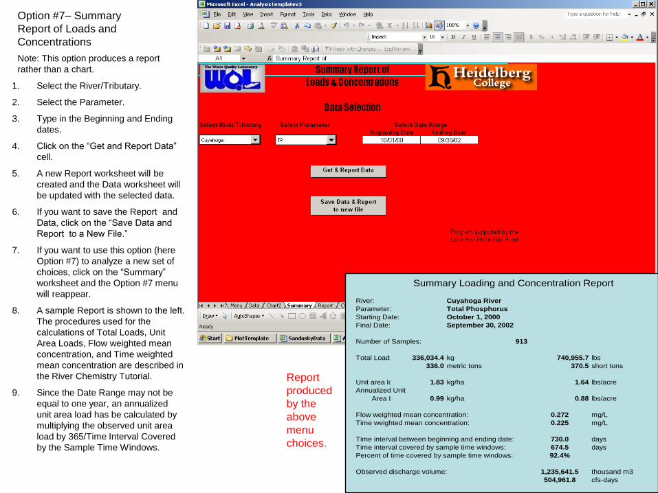
Option #7– Summary

Report of Loads and

Concentrations

Note: This option produces a report

rather than a chart.


2. Select the Parameter.


dates.

4. Click on the “Get and Report Data”

cell.

5. A new Report worksheet will be



6. If you want to save the Report and

Data, click on the “Save Data and

Report to a New File.”



choices, click on the “Summary”


will reappear.

8. A sample Report is shown to the left.

The procedures used for the

calculations of Total Loads, Unit

Area Loads, Flow weighted mean

concentration, and Time weighted

mean concentration are described in

the River Chemistry Tutorial.

9. Since the Date Range may not be

equal to one year, an annualized

unit area load has be calculated by

multiplying the observed unit area

load by 365/Time Interval Covered

by the Sample Time Windows.

Maumee River 10/1/1994 - 9/30/2004

1.0

10.0

100.0

1000.0

10000.0

100000.0

0% 10% 20% 30% 40% 50% 60% 70% 80% 90% 100%

Percent of time flow is exceeded

Fo

w

(cfs

)

0%

10%

20%

30%

40%

50%

60%

70%

80%

90%

100%

Pe

rce

nt

of

tota

l N

O2

3 lo

ad

Flow NO23

Chart

produced

by the

above

menu

choices.

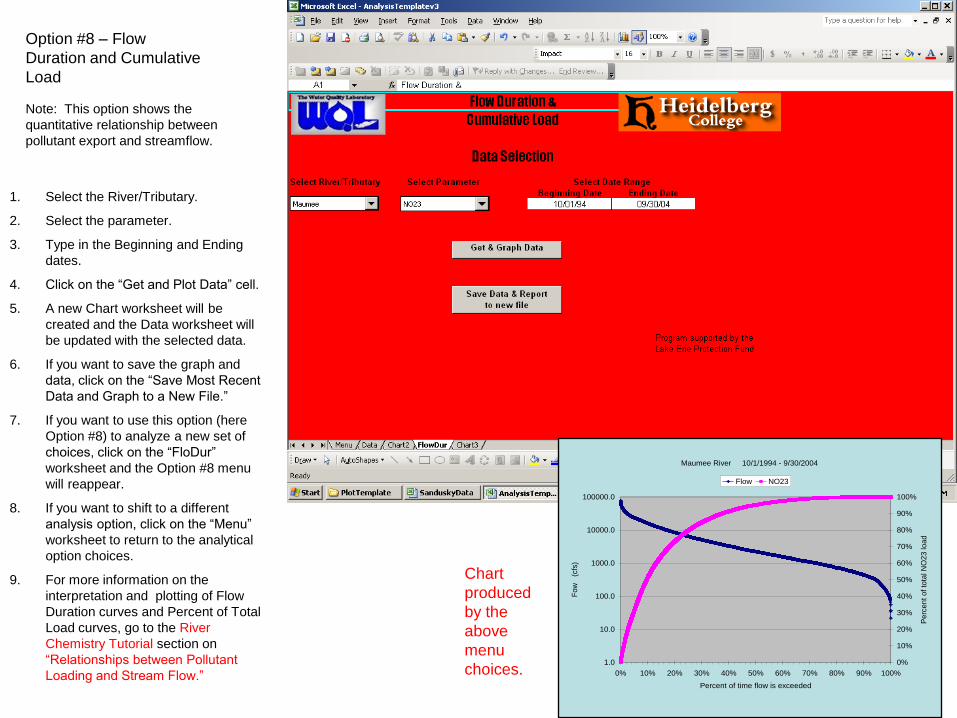
Option #8 – Flow

Duration and Cumulative

Load

Note: This option shows the

quantitative relationship between

pollutant export and streamflow.




dates.










choices, click on the “FloDur”


will reappear.




option choices.

9. For more information on the

interpretation and plotting of Flow

Duration curves and Percent of Total

Load curves, go to the River

Chemistry Tutorial section on

“Relationships between Pollutant

Loading and Stream Flow.”

Some additional characteristics of the Analysis

Templatev3 program

1. The workbooks that are produced to save the Data

and Chart or Report outputs are labeled Workbook 1,

Workbook 2, Workbook 3, etc. by the Analysis

Template Program. Only the Chart or Report Pages

of those workbooks contain the name of the

river/tributary. The Data page does not contain name

of the River. It is advisable to open, save and

rename the Workbooks promptly after creating them.

2. The Data page contains all the data called for by the

selections you have made on the analysis option you

are using. These columns represent the output of the

“Get Data” portion of the program. This includes the

DateTime information for each sample.

The Data Page also contains the columns that are

produced by any calculations and sorts of the data

that are necessary for creating the Charts or Report

called for by the analysis option you are using.

3. Familiarity with the Excel Chart program will allow you

to modify any of the Charts produced by the

AnalysisTemplatev3 program. These modifications

can aid in further data interpretation or make the

Charts more useful for particular applications, such as

use in educational programs or reports.

Directions for using AnalysisTemplatev3

Documents

Transcript of Directions for using AnalysisTemplatev3