ORIGINAL ARTICLE

Effect of process parameters on cut quality of stainless steelof plasma arc cutting using hybrid approach

K. P. Maity & Dilip Kumar Bagal

Received: 10 August 2013 /Accepted: 27 October 2014 /Published online: 5 December 2014# Springer-Verlag London 2014

Abstract An optimization concept of the various ma-chining parameters for the plasma arc cutting procedureson AISI 316 stainless steel conducting a hybrid optimi-zation method has been carried out. A new compositionof response surface methodology and grey relationalanalysis coupled with principal component analysis hasbeen proposed to evaluate and estimate the effect ofmachining parameters on the responses. The major re-sponses selected for these analyses are kerf, chamfer,dross, surface roughness and material removal rate, andthe corresponding machining parameters concentratedfor this study are feed rate, current, voltage and torchheight. Thirty experiments were conducted on AISI 316stainless steel workpiece materials based on a face-centered central composite design. The experimentalresults obtained are applied in grey relational analysis,and the weights of the responses were evaluated by theprincipal component analysis and further evaluatedusing response surface method. The results show thatthe grey relational grade was significantly affected bythe machining parameters directly as well as with someinteractions. This method is straightforward with easyoperability, and the results have also been establishedby running confirmation tests. The premise attributesbeneficial knowledge for managing the machining pa-rameters to enhance the preciseness of machined partsby plasma arc cutting.

Keywords Grey relational grade . Plasma arc cutting .

Principal component analysis .Response surfacemethodology

AbbreviationsAISI American Iron and Steel InstituteCNC Computer numerical controlHV Vickers hardnessANN Artificial neural networkQstE High-strength steel gradeHardox Abrasion-resistant steel gradeMRR Material removal rateSR Surface roughnessRa Central line average roughnessEN European standard steel numberISO International Organization for StandardizationLB Lower-the-betterHB Higher-the-betterNB Nominal-the-bestP Probability valueANOVA Analysis of variancePAC Plasma arc cuttingA Feed rate (mm/min)B Current (ampere)C Voltage (volt)D Torch height (mm)CCD Central composite designF Statistic test valueHα Hypothesis3D Three-dimensionalRSM Response surface methodologyGRA Grey relational analysisPCA Principal component analysis

NomenclatureL18 Orthogonal array of 18 runsL30 Orthogonal array of 30 runs

K. P. Maity (*) :D. K. BagalDepartment of Mechanical Engineering, NIT Rourkela,Rourkela 769008, Odisha, Indiae-mail: kpmaity@gmail.com

D. K. Bagale-mail: dilipbagal90@gmail.com

Int J Adv Manuf Technol (2015) 78:161–175DOI 10.1007/s00170-014-6552-6

Y ResponseXi Singular term of input variableXii Square term of input variableXiXj Interaction term of input variableβo Regression coefficient of constant termβi Regression coefficient of singularβii Regression coefficients of squareβij Regression coefficients of interactionϵ Regression error coefficientXi*(k) Normalized value of the kth elementkth Element numberith Sequence numberX0b(k) Desired valuemax Xi*(k) Largest value of Xi(k)min Xi*(k) Smallest value of Xi(k)Xi(k) SequenceX0(k) Reference sequenceζ Distinguishing coefficientβk Weighting value of the kth performanceCov(xi(j)) Covariance of sequenceσxi(j) Standard deviation of sequence xi(j)σxi(l) Standard deviation of sequence xi(l)λ Eigenvalueλk EigenvalueVik EigenvectorYm1 First principal componentYm2 Second principal component

1 Introduction

Modern industry depends on the manipulation of heavy metaland alloys. Different cutting methods are used to form intospecified pieces for making infrastructure and machine tools.Plasma arc cutting was developed in the mid 1950s and wasprimarily used to cut stainless steel and aluminium alloys.Plasma is the fourth and the most highly energized state ofmatter. In fact, plasma looks and behaves like a high temper-ature gas but with a capability to conduct electricity [1]. Thebasic principle is that the arc formed between the electrodeand the work piece is constricted by a fine bore, copper nozzle.This increases the temperature and velocity of the plasmaemanating from the nozzle. The temperature of the plasma isin excess of 20,000 °C, and the velocity can approach thespeed of sound. When used for cutting, the plasma gas flow isincreased so that the deeply penetrating plasma jet cutsthrough the material and molten material is removed in theefflux plasma [2].

Plasma arc cutting involves a large number of processparameters. It requires optimization of the process parametersfor smooth operation of plasma arc cutting process. A numberof investigators have carried out the research in this direction[3]. Bhuvenesh et al. investigated the surface roughness and

material removal rate of AISI-1017 mild steel using manualplasma arc cutting machining by Taguchi methodology [4].They observed that the relationship between average materialremoval rate and average surface roughness is inversely pro-portional to each other. Kechagias and Billis modeled a para-metric design of computer numerical control (CNC)-con-trolled plasma arc cutting process of St. 37 carbon steel andAISI steel plates by using robust design of orthogonal arrayL18 (2

1×37) [5, 6]. Arc ampere is the most significant factor.The standoff distance is the most significant parameter. Theplate thickness is the least significant parameter in plasma arccutting process.

Gullu and Atici investigated the consequence of plasma arcparameters on the structure variation of AISI-304 and St. 52steel plates by Panasonic digital PRIOR optic microscope andVicker hardness measurement device for heat affected zoneand hardness, respectively. It was evident from the statisticalanalysis that the cutting speed was the most significant factorwhich affects the surface roughness [7]. After cutting, it isseen that hardness increases in the areas near the surface ofpart i.e. around 250–350 HVand decreases towards the core ofthe material [8]. Özek et al. performed a Fuzzy model forpredicting surface roughness in plasma cutting of AISI-4140steel plate [7]. Radovanovic and Madic modeled a parametricdesign of plasma arc cutting process by using ANN to predictsurface roughness. It is observed that surface roughness in-creases with increase in cutting speed, but decreases withincrease in cutting arc current. Good surface finish can beachieved in plasma arc cutting process of 8-mm thick platewhen cutting current and cutting speeds are set nearer to theirhigh and low level of the experimental range, respectively[9–11].

The proficiency of a manufacturing practice to produce adesired quality of cut and material removal rate depends onvarious parameters. The factors that bias output responses aremachining parameters, tool and workpiece material propertiesand cutting conditions. Therefore, it is important for the re-searchers to model and appraise the relationship amongroughness and the parameters affecting its value. The deter-mination of this correlation remains an open field of research,mainly on account of the advances in machining and materialtechnology and the feasible modeling techniques. In machin-ability review investigations, statistical design of experimentsis used quite extensively. Statistical design of experimentsassign to the process of planning the experiments so that theadequate data can be examined by statistical methods,resulting in precise and objective conclusions [12].Nemchinsky and Severance discussed the fundamentals ofplasma arc cutting process with physical reasoning [13].Salonitis and Vatousianos recently carried out an experimentalinvestigation of the plasma arc cutting process [14].

Yun and Na carried out an experiment about the realtime control of plasma arc cutting process by using

162 Int J Adv Manuf Technol (2015) 78:161–175

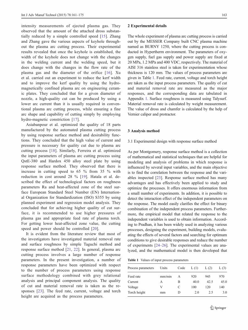
intensity measurements of ejected plasma gas. Theyobserved that the amount of the attached dross substan-tially reduced by a simple controlled speed [15]. Zhangand Zhang gave the various aspects of keyhole through-out the plasma arc cutting process. Their experimentalresults revealed that once the keyhole is established, thewidth of the keyhole does not change with the changesin the welding current and the welding speed, but itdoes change with the changes in the flow rate of theplasma gas and the diameter of the orifice [16]. Xuet al. carried out an experiment to reduce the kerf widthand to improve the kerf quality by using the hydro-magnetically confined plasma arc on engineering ceram-ic plates. They concluded that for a given diameter ofnozzle, a high-quality cut can be produced by using alower arc current than it is usually required in conven-tional plasma arc cutting process, while ensuring a finearc shape and capability of cutting simply by employinghydro-magnetic constriction [17].

Asiabanpour et al. optimized the quality of 18 partsmanufactured by the automated plasma cutting processby using response surface method and desirability func-tions. They concluded that the high value of current andpressure is necessary for quality cut due to plasma arccutting process [18]. Similarly, Ferreira et al. optimizedthe input parameters of plasma arc cutting process usingQstE-380 and Hardox 450 alloy steel plate by usingresponse surface method. They observed that there isincrease in cutting speed to 65 % from 35 % withreduction in cost around 28 % [19]. Hatala et al. de-scribed the effect of technological factors on roughnessparameters Ra and heat-affected zone of the steel sur-face European Standard Steel Number (EN) Internation-al Organization for Standardization (ISO) S355 by usingplanned experiment and regression model analysis. Theyconcluded that for achieving higher quality of cut sur-face, it is recommended to use higher pressures ofplasma gas and appropriate feed rate of plasma torch.For getting lower heat-affected zone value, the cuttingspeed and power should be controlled [20].

It is evident from the literature review that most ofthe investigators have investigated material removal rateand surface roughness by simple Taguchi method andresponse surface method [21, 22]. In general, plasma arccutting process involves a large number of responseparameters. In the present investigation, a number ofresponse parameters have been optimized with respectto the number of process parameters using responsesurface methodology combined with grey relationalanalysis and principal component analysis. The qualityof cut and material removal rate is taken as the re-sponses [23]. The feed rate, current, voltage and torchheight are acquired as the process parameters.

2 Experimental details

The whole experiment of plasma arc cutting process is carriedout by the MESSER Company built CNC plasma machinenamed as BURNY 1250, where the cutting process is con-ducted in Hypertherm environment. The parameters of oxy-gen supply, fuel gas supply and power supply are fixed at20 MPa, 1.2 MPa and 400 VDC, respectively. The material ofAISI 316 stainless steel is taken for experimentation whosethickness is 120 mm. The values of process parameters aregiven in Table 1. Feed rate, current, voltage and torch heightare taken as the input process parameters. The quality of cutand material removal rate are measured as the majorresponses, and the corresponding data are tabulated inAppendix 1. Surface roughness is measured using Talysurf.Material removal rate is calculated by weight measurement.The value of dross and chamfer is calculated by the help ofVernier caliper and protractor.

3 Analysis method

3.1 Experimental design with response surface method

As per Montgomery, response surface method is a collectionof mathematical and statistical techniques that are helpful formodeling and analysis of problems in which response isinfluenced by several input variables, and the main objectiveis to find the correlation between the response and the vari-ables inspected [23]. Response surface method has manyadvantages and has effectively been applied to study andoptimize the processes. It offers enormous information froma small number of experiments. In addition, it is possible todetect the interaction effect of the independent parameters onthe response. The model easily clarifies the effect for binarycombination of the independent process parameters. Further-more, the empirical model that related the response to theindependent variables is used to obtain information. Accord-ing to Pradhan, it has been widely used in analyzing variousprocesses, designing the experiment, building models, evalu-ating the effects of several factors and searching for optimumconditions to give desirable responses and reduce the numberof experiments [24–26]. The experimental values are ana-lyzed, and the mathematical model is then developed that

Table 1 Values of input process parameters

Process parameters Units Code L (1) L (2) L (3)

Feed rate mm/min A 920 945 970

Current A B 40.0 42.5 45.0

Voltage V C 100 120 140

Torch height mm D 2.0 2.5 3.0

Int J Adv Manuf Technol (2015) 78:161–175 163

illustrates the relationship between the process variable andresponse. The following second-order model explains thebehavior of the system:

Y ¼ β0 þXi¼1

k

βiX i þXi¼1

k

βiiX2i þ

Xi; j¼1;i≠ j

k

βi jX iX j þ ∈ ð1Þ

where Y is the corresponding response, Xi is the inputvariables and Xii and XiXj are the squares and interactionterms, respectively, of these input variables. The unknownregression coefficients are β0, βi, βij and βii, and the error inthe model is depicted as ϵ [25]. The response surface methoddesign of matrix form is given in Appendix 1. The outputresponses of plasma arc cutting as per response surface meth-od are given in Appendix 2.

3.2 Data preprocessing

According to Fung, data preprocessing is the method of trans-ferring the original sequence to a comparable sequence, wherethe original data normalize to a range of 0 and 1 [28]. Gener-ally, three different kinds of data normalizations are carriedout to render the data, whether the lower-the-better (LB), thehigher-the-better (HB) or nominal-the-best (NB). For ‘higher-the-better’, characteristics such as productivity or materialremoval rate, the original sequence can be HB and should benormalized as follows [27]:

X i� kð Þ ¼ X i kð Þ−minX i kð Þ

maxX i kð Þ−minX i kð Þ ð2Þ

However, if the expectancy is as small as possible for thequality of cut such as mean surface roughness, chamfer, drossand kerf, then the original sequence should be normalized as‘lower-the-better’:

X i� kð Þ ¼ maxX i kð Þ−X i kð Þ

maxX i kð Þ−minX i kð Þ ð3Þ

Conversely, if a specific target value is to be achieved, thenthe original sequence will be normalized by the followingequation of NB:

X i� kð Þ ¼ 1−

X i kð Þ−minX 0b kð Þj jmaxX i kð Þ−X 0b kð Þ ð4Þ

where i=1,2,…,n; k=1,2,…,p; Xi*(k) is the normalizedvalue of the kth element in the ith sequence; X0b(k) is thedesired value of the kth quality characteristic; max Xi*(k) is thelargest value of Xi(k); min Xi*(k) is the smallest value of Xi(k);n is the number of experiments; and p is the number of qualitycharacteristics [28]. According to the type of characteristic,type of responses normalize the Appendix 2 as per aboveequation and the outcomes are tabulated in Appendix 3. As

the responses are of LB and HB types, there is no use ofEq. (4) in the present calculation.

3.3 Grey relational coefficient and grey relational grade

After normalizing the data, usually grey relational coefficientis calculated to display the relationship between the optimaland actual normalized experimental results. The grey relation-al coefficient can be expressed as [29–31]:

γi kð Þ ¼ γ X 0 kð Þð − X i kð Þð Þ ¼ Δminþ ζΔmax

Δ0;i kð Þ þ ζΔmaxi ¼ 1; 2; 3;…; n; k ¼ 1; 2; 3;…; p

ð5Þ

where is Δ0,i(k)=|X0(k)−Xi(k)| the difference of the abso-lute value called deviation sequence of the reference sequenceX0(k) and comparability Xi(k). ζ is the distinguishing coeffi-cient or identification coefficient in which the value range is 0≤ ζ ≤1. In general, it is set to 0.5 as optimistic value in normaldistribution; hence, same is adopted in this study. The aim ofdefining the grey relational coefficient is to express the rela-tional degree between the reference sequence X0(k) and thecomparability sequences Xi(k), where i=1,2,…,m and k=1,2,…,nwithm=30 and n=3 in this study [32]. The computeddeviation sequences of the normalized values are tabulated inAppendix 4.

The grey relational grade is a weighting sum of the greyrelational coefficients and it is defined as [31]:

γ x0; xið Þ ¼Xk¼1

n

βk x0; xið Þ ð6Þ

where βk represents the weighting value of the kth perfor-mance characteristic and [32]

Xk¼1

n

βk ¼ 1 ð7Þ

3.4 Principal component analysis

Principal component analysis is a mathematical approach thatconverts a set of observations of probably correlated variablesinto a set of values of uncorrelated variables. It was inventedvery early and later mostly used as a tool in investigative dataanalysis and for the formation of predictive models. Principalcomponent analysis can be done by eigenvalue decompositionof a data covariance matrix or singular value decomposition of adata matrix. It is used for identifying patterns in data andexpressing the data in such away as to highlight their similaritiesand differences [33]. The main advantage of principal compo-nent analysis is that once the patterns in data have been identi-fied, the data can be compressed, i.e. by reducing the number of

164 Int J Adv Manuf Technol (2015) 78:161–175

dimensions, without much loss of information. The explicitgoals of principal component analysis are the following:

1. To extract the most significant information from the data,2. To squeeze the size of the data set by keeping only the

significant,3. To simplify the explanation of the data set, and4. To analyze the structure of the observations and the

variables.

The procedure is described as follows [33]:

1. The original multiple quality characteristic array

X ¼

x1 1ð Þ x1 2ð Þ … … x1 nð Þx2 1ð Þ x2 2ð Þ … … x2 nð Þ: : … … :: : … … :

xm 1ð Þ xm 2ð Þ … … xm nð Þ

266664

377775 ð8Þ

i=1,2,…,m; j=1,2,…,n [34]where m is the number of experiment and n is the

number of the response. In the present work, x is the greyrelational coefficient of each response and m=30and n=3.

2. Correlation coefficient arrayThe correlation coefficient array is evaluated as

follows:

Rjl ¼ Cov xi jð Þ; xi lð Þð Þσxi jð Þ � σxi lð Þ

� �

j ¼ 1; 2; 3;…;ml ¼ 1; 2; 3;…; n

ð9Þ

where Cov(xi(j)), xi(l) is the covariance of se-quences xi(l) and xi(l), σxi(j) is the standard devia-tion of sequence xi(j) and σxi(l) is the standarddeviation of sequence xi(l).

3. Determining the eigenvalues and eigenvectorsThe eigenvalues and eigenvectors are determined from

the correlation coefficient array:

R−λkImð ÞV ik ¼ 0 ð10Þ

where λ is the eigenvalue ∑k¼1

n

λk ¼ n; k ¼ 1; 2; 3;…;

n and Vik=[ak1,ak2,ak3,…,akm]T is the eigenvectors cor-

responding to the eigenvalue λk. The eigenvalues and itsvariation are shown in (Table 2 as per Eq. 10 ).

4. Principal componentsThe uncorrelated principal component is formulated as:

Ymk ¼Xi¼1

n

xm ið Þ⋅V ik ð11Þ

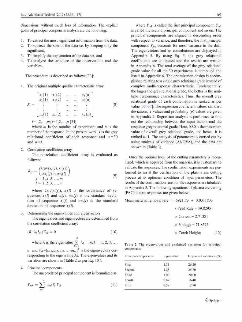
where Ym1 is called the first principal component, Ym2is called the second principal component and so on. Theprincipal components are aligned in descending orderwith respect to variance, and therefore, the first principalcomponent Ym1 accounts for most variance in the data.The eigenvectors and its contributions are displayed inAppendix 5. By using Eq. 5, the grey relationalcoefficients are computed and the results are writtenin Appendix 6. The total average of the grey relationalgrade value for all the 30 experiments is computed andlisted in Appendix 6. The optimization design is accom-plished relating to a single grey relational grade instead ofcomplex multi-response characteristic. Fundamentally,the larger the grey relational grade, the better is the mul-tiple performance characteristics. Thus, the overall greyrelational grade of each combination is ranked as pervalue [35–37]. The regression coefficient values, standarddeviations, T values and probability (p) values are givenin Appendix 7. Regression analysis is performed to findout the relationship between the input factors and theresponse grey relational grade. Here, 0.80 is the maximumvalue of overall grey relational grade, and hence, it isranked as 1. The analysis of parameters is carried out byusing analysis of variance (ANOVA), and the data areshown in (Table 3).

Once the optimal level of the cutting parameters is recog-nized, which is acquired from the analysis, it is customary tovalidate the responses. The confirmation experiments are per-formed to assist the verification of the plasma arc cuttingprocess at its optimum condition of input parameters. Theresults of the confirmation runs for the responses are tabulatedin Appendix 3. The following equations of plasma arc cutting(PAC) output responses are given below:

Mean material removal rate ¼ 6921:73 þ 0:0311833

� Feed Rate − 39:8295

� Current − 2:71381

� Voltage − 71:8525

� Torch Height; ð12Þ

Table 2 The eigenvalues and explained variation for principalcomponents

Principal components Eigenvalue Explained variations (%)

First 1.31 26.20

Second 1.28 25.70

Third 1.00 20.00

Fourth 0.82 16.40

Fifth 0.59 12.70

Int J Adv Manuf Technol (2015) 78:161–175 165

Mean surface roughness ¼ 9:1349 þ 0:0503167

� Feed Rate − 1:52617

� Current− 0:171021

� Voltage þ 4:2075

� Torch Height;

Chamfer ¼ 1:82142 − 0:00045

� Feed Rate − 0:00683333

� Current − 0:00139583� Voltage

þ 0:220833� Torch Height;

Dross ¼ 46:2527 − 0:0262 � Feed Rate − 0:381667

� Current − 0:020625� Voltage þ 1:08833

� Torch Height;

Table 3 The ANOVA table

*p≤0.05

Sources DF Seq. SS Adj. SS Adj. MS F P Percent contribution

Regression 14 0.30 0.30 0.02 1.07 0.45 49.90

Linear 4 0.13 0.12 0.03 1.52 0.25 22.65

A 1 0.02 0.02 0.02 0.88 0.36 3.51

B 1 0.02 0.03 0.03 1.46 0.25 3.39

C 1 0.01 0.00 0.00 0.02 0.89 1.05

D 1 0.09 0.09 0.09 4.62 0.05* 14.70

Square 4 0.06 0.06 0.01 0.71 0.60 9.53

A×A 1 0.00 0.01 0.01 0.45 0.51 0.50

B×B 1 0.03 0.04 0.04 1.98 0.18 5.48

C×C 1 0.00 0.00 0.00 0.03 0.86 0.00

D×D 1 0.02 0.02 0.02 1.06 0.32 3.55

Interaction 6 0.11 0.11 0.02 0.88 0.53 17.71

A×B 1 0.01 0.01 0.01 0.34 0.57 1.12

A×C 1 0.00 0.00 0.00 0.04 0.84 0.15

A×D 1 0.09 0.09 0.09 4.53 0.05* 15.13

B×C 1 0.00 0.00 0.00 0.02 0.89 0.00

B×D 1 0.00 0.00 0.00 0.02 0.90 0.00

C×D 1 0.01 0.01 0.01 0.36 0.56 1.19

Residual error 15 0.30 0.30 0.02 5.10

Lack-of-fit 10 0.20 0.20 0.02 0.98 0.54 33.22

Pure error 5 0.10 0.10 0.02 16.89

Total 29 0.60

166 Int J Adv Manuf Technol (2015) 78:161–175

4%4%

1%

16%1%0%

17%

0%0%1%

56%

% Contibution of parameters on overall grey grades

FEED RATE CURRENTVOLTAGE TORCH HEIGHTFEED RATE*CURRENT FEED RATE*VOLTAGEFEED RATE*TORCH HEIGHT CURRENT*VOLTAGECURRENT*TORCH HEIGHT VOLTAGE*TORCH HEIGHTResidual Error

Fig. 1 3D pie chart of percentage contribution of input variables onoverall grey relational grades

ð13Þ

ð14Þ

ð15Þ

Int J Adv Manuf Technol (2015) 78:161–175 167

3210-1-2-3

99

95

90

80

70

60504030

20

10

5

1

Standardized Residual

Perc

ent

Normal Probability Plot(response is Overall Grey Relational Grade)

0.70.60.50.40.3

2

1

0

-1

-2

Fitted Value

Stan

dard

ized

Res

idua

l

Versus Fits(response is Overall Grey Relational Grade)

(a) (b)

0.20.10.0-0.1-0.2

10

8

6

4

2

0

Standardized Residual

Freq

uenc

y

Histogram(response is Overall Grey Relational Grade)

30282624222018161412108642

2

1

0

-1

-2

Observation Order

Stan

dard

ized

Res

idua

l

Versus Order(response is Overall Grey Relational Grade)

(c) (d)Fig. 2 Plot of residuals of overall grey relational grade

995970945920895

0.7

0.6

0.5

0.4

0.3

47.545.042.540.037.5

16014012010080

0.7

0.6

0.5

0.4

0.3

3.53.02.52.01.5

Feed Rate

Mea

n

Current

Voltage Torch Height

Main Effects Plot for Overall Grey Relational GradeFig. 3 Main effect plot of overallgrey relational grade

Kerf ¼ 10:436 − 0:00596667

� Feed Rate − 0:0693333

� Current − 0:00075� Voltage þ 0:435

� Torch Height; ð16Þ

4 Results and discussions

Cutting the stainless steel plates is still more defying than thatof other steel metals due to the difference in the physical,mechanical and metallurgical properties of the metals to becut. Proper choice of mechanism and process variables are,

168 Int J Adv Manuf Technol (2015) 78:161–175

Feed Rate

Curren

t

990980970960950940930920910900

47

46

45

44

43

42

41

40

39

38

Voltage 120Torch Height 2.5

Hold Values

>–––< 0.5

0.5 0.60.6 0.70.7 0.8

0.8

GradeRelationalGreyOverall

Contour Plot of Overall Grey Relational Grade vs Current, Feed Rate

Feed Rate

Volta

ge

990980970960950940930920910900

160

150

140

130

120

110

100

90

80

Current 42.5Torch Height 2.5

Hold Values

>––––––< 0.450

0.450 0.4750.475 0.5000.500 0.5250.525 0.5500.550 0.5750.575 0.600

0.600

GradeRelational

Overall Grey

Contour Plot of Overall Grey Relational Grade vs Voltage, Feed Rate

(a) (b)

Feed Rate

TorchHeigh

t

990980970960950940930920910900

3.5

3.0

2.5

2.0

1.5

Current 42.5Voltage 120

Hold Values

>––––< 0.2

0.2 0.40.4 0.60.6 0.80.8 1.0

1.0

GradeRelational

GreyOverall

Contour Plot of Overall Grey Relational vs Torch Height, Feed Rate

Current

Volta

ge

47464544434241403938

160

150

140

130

120

110

100

90

80

Feed Rate 945Torch Height 2.5

Hold Values

>–––––< 0.45

0.45 0.500.50 0.550.55 0.600.60 0.650.65 0.70

0.70

GradeRelational

Overall Grey

Contour Plot of Overall Grey Relational Grade vs Voltage, Current

(c) (d)

Current

TorchHeigh

t

47464544434241403938

3.5

3.0

2.5

2.0

1.5

Feed Rate 945Voltage 120

Hold Values

>––––< 0.5

0.5 0.60.6 0.70.7 0.80.8 0.9

0.9

GradeRelationalGreyOverall

Contour Plot of Overall Grey Relational Grade vs Torch Height, Current

Voltage

TorchHeigh

t

1601501401301201101009080

3.5

3.0

2.5

2.0

1.5

Feed Rate 945Current 42.5

Hold Values

>–––< 0.4

0.4 0.50.5 0.60.6 0.7

0.7

GradeRelationalGreyOverall

Contour Plot of Overall Grey Relational Grade vs Torch Height, Voltage

(e) (f)Fig. 4 Contour plot of interaction terms vs. overall grey relational grade

therefore, obligatory to make the cuts with good quality.Therefore, plasma arc cutting of stainless steel metals hasincreasing demand due to the higher penetration rates andwith the benefits of high cutting speed providing higherproductivity. This paper demonstrated a bid for devel-opment of mathematical models of the plasma arc cut-ting process based on response surface methodology.Parameter design of response surface methodology be-ing simple and cheap is adopted for in-depth study tounderstand process parameters and their interaction ef-fects on responses like accuracy of dimensions in dif-ferent directions of PAC built parts with minimum ex-perimental runs [38]. To maintain a high production rate

and admissible quality of cut devices, the machiningprocess parameters of PAC must be optimized [39].

From the design of experiments and due to a broad range ofinput process parameters, the present work is contoured tofour factors, three levels and an L30 orthogonal array designmatrix to simplify the present dilemma. In this present study,30 experiments are carried out based on response surfacemethod with a face-centered central composite design(CCD). Here, the MINITAB version 16 software is used tooptimize the experimental data, and this software is a well-efficient statistical tool which helps to analyze the influence ofinput parameters on output responses of whole experimentaldesign.

Int J Adv Manuf Technol (2015) 78:161–175 169

4844

0.4

0.6

40900

0.8

950 1000

Current

GRG

Feed Rate

Voltage 120

Torch Height 2.5

Hold Values

Surface Plot of Overall GRG vs Current, Feed Rate

1600.45120

0.50

0.55

900

0.60

80950 1000

GRG

Voltage

Feed Rate

Current 42.5

Torch Height 2.5

Hold Values

Surface Plot of Overall GRG vs Voltage, Feed Rate

3.63.0

0.3

2.4

0.6

90

0.9

1.8950

1000

GRG

Torch Height

Feed Rate

Current 42.5

Voltage 120

Hold Values

Surface Plot of Overall GRG vs Torch Height, Feed Rate

160

120

0.5

0.6

40

0.7

8044 48

GRG

Voltage

Current

Feed Rate 945

Torch Height 2.5

Hold Values

Surface Plot of Overall GRG vs Voltage, Current

(a) (b)

(c) (d)

(e) (f)

3.63.0

0.4 2.4

0.6

0.8

40 1.844 48

GRG

Torch Height

Current

Feed Rate 945

Voltage 120

Hold Values

Surface Plot of Overall GRG vs Torch Height, Current

3.63.0

0.4

2.4

0.5

0.6

80

0.7

1.8120160

GRG

Torch Height

Voltage

Feed Rate 945

Current 42.5

Hold Values

Surface Plot of Overall GRG vs Torch Height, Voltage

Fig. 5 Surface plot of interaction terms vs. overall grey relational grade

The regression analysis is carried out to inspect how muchis the goodness of relationship in between process variablesand the overall grey relational grade in the experiment. FromAppendix 7, it can be concluded that the torch height and theinteraction of feed rate and torch height are the most influenc-ing character as theP value comes 0.05. The ANOVA analysisis applied to test the adequacy of the design by observing the Pvalue for the F statistic under the 95 % confidence interval.According to the null hypothesis, if the value of P is less thanor equal to 0.05, then it is concluded that the Hα is very muchexact and the treatments have statistically significant effect onexperiment. From the last column of Appendix 2, it is seenthat the torch height is the most significant term due to itsmaximum percentage contribution, i.e. 14.70 % followed byfeed rate with 3.51 % and current and voltage with 3.39 and1.05 %, respectively. Similarly, analysis is carried out todetermine the percentage contribution of the square and theinteraction terms of input process parameters from this table.Again, from this column of Appendix 7, it can be predictedthat the residual error of experiment has only 5.10 % contri-bution to the experiment. Then, the percentage of contributionof lack-of-fit and pure error is listed as 33.22 and 16.89 %,respectively, which shows the deficiency in fitting the data.

From the 3D pie chart of Fig. 1, it is indicated thatthe torch height has the highest impact on experimentalresults. The residual plots of input variable of plasmaarc cutting process have been plotted in Fig. 3. FromFig. 2a of normal probability plot, it can be understoodthat all the data follow a normal distribution as all thepoints were placed near the straight line. It can be seenthat the process parameters of plasma arc cutting pro-cess have a fruitful significance on experiment as thereis a large angled slope of straight line in the graph. Thefitted value vs. standardized residual of overall greyrelational grade is plotted in Fig. 2b where a randomdistribution is observed for the model. Here, the stan-dardized residual distribution pursues that the indepen-dent patterns are normally placed on each side of thereference line. Now, from the histogram plot of stan-dardized residuals in Fig. 2c, it is inferred that all thecolumns are performed in a normal distribution with itsmean and standard deviation. Figure 2d shows that theplot in between the observed run order and the stan-dardized residuals in which it can be visually under-stood that the maximum and minimum influence of

process parameters on responses occurred at the 17thand 25th run order, respectively.

The main effect plot of overall grey relational gradeis presented in Fig. 3. This obtains the optimal para-metric setting of process parameters in plasma arc cut-ting machining operation. From the main effect plot, itis concluded that the optimistic overall grey relationalgrade can be achieved with feed rate=970 mm/min,current=47.5 A, voltage=140 V and torch height=1.5 mm respectively.

The counter plots of interaction terms at their averagelevel vs. overall grey relational grade are found in Fig. 4.Mainly, the shapes of counter plots might be elliptical orsaddle form which indicates that the combination of eachvariable is significant except voltage vs. current plot be-cause of the lowest value of overall grey relational gradeobtained in the middle region of current, which can beseen in Fig. 4d.

Similarly, the 3D surface plot of the abovementioned inter-action terms can be exerted in Fig. 5. It is to be noted that allother terms are taken into account at their average value.Finally, the confirmation test has been carried out at theoptimum condition of plasma arc cutting process parameterswhich is to confirm the feasibility of the correct optimalsetting on responses of the experiment. The outcomes of theconfirmation test for the mean material removal rate and thequality of cut values are computed in Table 4. Here, thedistance between nozzle of torch and workpiece is the crucialfactor in this experiment. From the ANOVA analysis, it isevident that the interaction of feed rate and torch height is alsoinfluenced to the abovementioned outputs.

From the above descriptive analysis, evidently, the bestdesign is becoming one primary challenge of technologymarket. In this paper, the optimal values of process parametershave been numerically found out using the quadratic model ofresponse surface methodology (RSM). Since time and cost arecomprised while operating the experimental runs, it is relevantto reduce the number of runs while not compromising thedesired goals [40].

5 Conclusion

This paper furnishes the findings of an experimentalinvestigation into the effect of feed rate, current, voltage

Table 4 Conformation results for mean material removal rate and the quality of cut

Best combination Experimental value Predicted value

Mean MRR(mm2/min)

Mean SR(μm)

Chamfer(mm)

Dross(mm2)

Kerf(mm)

Mean MRR(mm2/min)

Mean SR(μm)

Chamfer(mm)

Dross(mm2)

Kerf(mm)

A B C D

970 47.50 140 1.5 3987.47 62.94 1.48 1.72 1.95 4572.4 32.18 1.20 1.45 1.90

170 Int J Adv Manuf Technol (2015) 78:161–175

and torch height on the characteristic of cut when ma-chining AISI 316 stainless steel by plasma. The specificproblems of PAC have been analyzed. Response surfacemethod coupled with grey relational analysis and prin-cipal component analysis has been carried out to opti-mize plasma arc cutting processes with multi-objectivecriteria. The best possible optimum conditions of thisprocess are the following: 970 mm/min of feed rate,47.5 A of current, 140 V of voltage and 1.5 mm oftorch height. Torch height as well as interaction of torchheight with feed rate is the most influencing parametersin plasma arc cutting machining. The shortened quadrat-ic models developed using the combinatorial plea ofRSM and grey relational analysis (GRA) with principalcomponent analysis (PCA) were reasonably accurate andcan be used for prediction within the limits of thefactors investigated.

Appendix 1

Appendix 2

Table 6 Output responses of plasma arc cutting process

Run order Mean materialremoval rate

Mean surfaceroughness

Chamfer Dross Kerf

1 4891.10 58.16 1.83 3.63 2.73

2 3992.62 46.49 1.01 0.80 3.44

3 5541.59 51.81 1.52 9.57 2.64

4 4494.18 25.82 1.42 4.26 2.70

5 5497.43 71.42 1.88 8.26 3.53

6 5082.01 41.88 1.00 7.00 3.30

7 3842.59 62.86 1.05 4.29 2.38

8 4865.14 69.52 1.64 7.63 3.41

9 5345.53 51.13 1.52 8.52 2.61

10 5678.41 32.08 1.83 0.45 2.73

11 3061.77 37.48 1.24 3.00 3.48

12 3929.05 63.29 1.47 1.74 1.93

13 3905.86 72.62 1.58 4.56 2.39

14 5670.24 52.73 1.05 5.25 2.63

15 3489.34 35.60 1.62 2.73 3.73

16 4995.12 63.60 1.10 6.34 2.53

17 5427.69 34.60 1.53 1.74 3.58

18 4223.34 56.61 1.08 6.43 2.65

19 4854.34 71.30 1.63 3.83 3.41

20 5030.29 54.97 1.38 5.27 2.64

21 4072.35 62.76 1.97 8.57 2.34

22 5448.16 34.18 1.68 4.56 2.57

23 4402.74 43.74 1.47 8.43 2.62

24 5470.08 52.35 1.64 9.03 3.73

25 4415.95 66.97 1.78 5.89 2.93

26 5520.10 26.57 1.93 8.52 2.28

27 4649.92 45.13 1.43 3.67 2.04

28 3805.88 44.59 1.67 7.27 3.16

29 5453.33 63.04 1.24 5.79 2.27

30 5538.55 61.25 1.52 8.53 3.07

Table 5 Response surface method design with input parameters

Std. order Run order Feed rate Current Voltage Torch height

18 1 945 42.5 120 2.5

7 2 920 45.0 140 2.0

20 3 945 42.5 120 2.5

3 4 920 45.0 100 2.0

9 5 920 40.0 100 3.0

5 6 920 40.0 140 2.0

2 7 970 40.0 100 2.0

11 8 920 45.0 100 3.0

19 9 945 42.5 120 2.5

4 10 970 45.0 100 2.0

17 11 945 42.5 120 2.5

8 12 970 45.0 140 2.0

13 13 920 40.0 140 3.0

16 14 970 45.0 140 3.0

15 15 920 45.0 140 3.0

12 16 970 45.0 100 3.0

14 17 970 40.0 140 3.0

6 18 970 40.0 140 2.0

10 19 970 40.0 100 3.0

1 20 920 40.0 100 2.0

29 21 945 42.5 120 2.5

30 22 945 42.5 120 2.5

25 23 945 42.5 80 2.5

23 24 945 37.5 120 2.5

Table 5 (continued)

Std. order Run order Feed rate Current Voltage Torch height

22 25 995 42.5 120 2.5

26 26 945 42.5 160 2.5

24 27 945 47.5 120 2.5

28 28 945 42.5 120 3.5

27 29 945 42.5 120 1.5

21 30 895 42.5 120 2.5

Int J Adv Manuf Technol (2015) 78:161–175 171

Appendix 3 Appendix 4

Table 7 Normalized values for mean material removal rate and thequality of cut

Run order Mean materialremoval rate

Mean surfaceroughness

Chamfer Dross Kerf

1 0.70 0.31 0.15 0.65 0.56

2 0.36 0.56 1.00 0.96 0.16

3 0.95 0.44 0.46 0.00 0.61

4 0.55 1.00 0.57 0.58 0.58

5 0.93 0.03 0.09 0.14 0.11

6 0.77 0.66 1.00 0.28 0.24

7 0.30 0.21 0.95 0.58 0.75

8 0.69 0.07 0.34 0.21 0.18

9 0.87 0.46 0.46 0.12 0.63

10 1.00 0.87 0.15 1.00 0.56

11 0.00 0.75 0.76 0.72 0.14

12 0.33 0.20 0.52 0.86 1.00

13 0.32 0.00 0.41 0.55 0.74

14 1.00 0.42 0.95 0.47 0.61

15 0.16 0.79 0.36 0.75 0.00

16 0.74 0.19 0.90 0.35 0.67

17 0.90 0.81 0.46 0.86 0.08

18 0.44 0.34 0.92 0.34 0.60

19 0.69 0.03 0.36 0.63 0.18

20 0.75 0.38 0.61 0.47 0.61

21 0.39 0.21 0.00 0.11 0.77

22 0.91 0.82 0.30 0.55 0.64

23 0.51 0.62 0.52 0.13 0.62

24 0.92 0.43 0.34 0.06 0.00

25 0.52 0.12 0.20 0.40 0.45

26 0.94 0.98 0.05 0.11 0.81

27 0.61 0.59 0.56 0.65 0.94

28 0.28 0.60 0.31 0.25 0.31

29 0.91 0.20 0.75 0.41 0.81

30 0.95 0.24 0.47 0.11 0.37

Table 8 The deviation sequences for mean material removal rate and thequality of cut

Run order Mean materialremoval rate

Mean surfaceroughness

Chamfer Dross Kerf

1 0.30 0.69 0.85 0.35 0.44

2 0.64 0.44 0.00 0.04 0.84

3 0.05 0.56 0.54 1.00 0.39

4 0.45 0.00 0.43 0.42 0.42

5 0.07 0.97 0.91 0.86 0.89

6 0.23 0.34 0.00 0.72 0.76

7 0.70 0.79 0.05 0.42 0.25

8 0.31 0.93 0.66 0.79 0.82

9 0.13 0.54 0.54 0.88 0.37

10 0.00 0.13 0.85 0.00 0.44

11 1.00 0.25 0.24 0.28 0.86

12 0.67 0.80 0.48 0.14 0.00

13 0.68 1.00 0.59 0.45 0.26

14 0.00 0.58 0.05 0.53 0.39

15 0.84 0.21 0.64 0.25 1.00

16 0.26 0.81 0.10 0.65 0.33

17 0.10 0.19 0.54 0.14 0.92

18 0.56 0.66 0.08 0.66 0.40

19 0.31 0.97 0.64 0.37 0.82

20 0.25 0.62 0.39 0.53 0.39

21 0.61 0.79 1.00 0.89 0.23

22 0.09 0.18 0.70 0.45 0.36

23 0.49 0.38 0.48 0.87 0.38

24 0.08 0.57 0.66 0.94 1.00

25 0.48 0.88 0.80 0.60 0.55

26 0.06 0.02 0.95 0.89 0.19

27 0.39 0.41 0.44 0.35 0.06

28 0.72 0.40 0.69 0.75 0.69

29 0.09 0.80 0.25 0.59 0.19

30 0.05 0.76 0.53 0.89 0.63

172 Int J Adv Manuf Technol (2015) 78:161–175

Appendix 5

Appendix 6

Table 9 The eigenvectors for principal components and contribution

Outputs Eigenvectors

Principalcomponentanalysis(1)

Principal componentanalysis(2)

Principal componentanalysis(3)

Principal componentanalysis(4)

Principal componentanalysis(5)

%

Mean material removal rate −0.59 0.27 0.05 0.67 −0.34 35

Mean surface roughness 0.04 0.76 −0.11 0.06 0.63 00

Chamfer 0.53 −0.23 0.41 0.66 0.25 29

Dross 0.58 0.49 −0.07 −0.01 −0.65 33

Kerf 0.16 −0.22 −0.90 0.33 0.07 03

Table 10 Grey relational coefficient, grey relational grade and rank of the mean material removal rate and the quality of cut

Sl. no. Grey relational coefficient Overall grey relational grade Rank

Material removal rate Surface roughness Chamfer Dross Kerf

1 0.62 0.42 0.37 0.59 0.53 0.53 16

2 0.44 0.53 0.99 0.93 0.37 0.74 4

3 0.91 0.47 0.48 0.33 0.56 0.49 19

4 0.52 1.00 0.54 0.54 0.54 0.57 13

5 0.88 0.34 0.36 0.37 0.36 0.41 26

6 0.69 0.59 1.00 0.41 0.40 0.66 6

7 0.42 0.39 0.91 0.54 0.67 0.59 11

8 0.62 0.35 0.43 0.39 0.38 0.42 23

9 0.80 0.48 0.48 0.36 0.57 0.50 18

10 1.00 0.79 0.37 1.00 0.53 0.75 2

11 0.33 0.67 0.68 0.64 0.37 0.46 20

12 0.43 0.38 0.51 0.78 1.00 0.58 12

13 0.42 0.33 0.46 0.53 0.66 0.43 22

14 0.99 0.47 0.90 0.49 0.56 0.80 1

15 0.37 0.71 0.44 0.67 0.33 0.41 24

16 0.66 0.38 0.84 0.44 0.60 0.66 7

17 0.84 0.73 0.48 0.78 0.35 0.74 3

18 0.47 0.43 0.86 0.43 0.56 0.55 15

19 0.61 0.34 0.44 0.57 0.38 0.56 14

20 0.67 0.45 0.56 0.49 0.56 0.62 9

21 0.45 0.39 0.33 0.36 0.69 0.20 30

22 0.85 0.74 0.42 0.53 0.58 0.61 10

23 0.51 0.57 0.51 0.36 0.57 0.39 27

24 0.86 0.47 0.43 0.35 0.33 0.45 21

25 0.51 0.36 0.38 0.46 0.47 0.39 28

Int J Adv Manuf Technol (2015) 78:161–175 173

Appendix 7

References

1. Hatala IM, Orlovský II (2009)Mathematical modelling of plasma arccutting technological process. 13th International Research/ExpertConference “Trends in the Development of Machinery andAssociated Technology”. pp 65–68

2. Rana K, Kaushik P, Chaudhary S (2013) Optimization of plasma arccutting by applying Taguchi Method. Int J Enhanc Res Sci TechnolEng 2:106–110

3. Kumar P, Ahuja IPS, Singh R (2012) Application of fusion deposi-tion modelling for rapid investment casting—a review. Int J MaterEng Innov 3:204. doi:10.1504/IJMATEI.2012.049254

4. Bhuvenesh R, Norizaman MH, Manan MSA (2012) Surface rough-ness andMRR effect onmanual plasma arc cuttingmachining.WorldAcad Sci Eng Technol 62:503–506

5. Kechagias J, Billis M (2010) A parameter design of CNC plasma-arccutting of carbon steel plates using robust design. StergiosMaropoulos 1:315–326

6. Concetti A (2011) Integrated approaches for designing and optimiz-ing thermal plasma processing for metal cutting and material treat-ment. 1–197

7. Özek C, Çaydaş U, Ünal E (2012) A fuzzy model for predictingsurface roughness in plasma arc cutting of AISI 4140 steel. MaterManuf Process 27:95–102. doi:10.1080/10426914.2011.551952

8. Gullu A, Atici U (2006) Investigation of the effects of plasma arcparameters on the structure variation of AISI 304 and St 52 steels.Mater Des 27:1157–1162. doi:10.1016/j.matdes.2005.02.014

9. Radovanovic M, Madic M (2011) Modeling the plasma arc cuttingprocess using ANN. Nonconventional Technol Rev 4:43–48

10. PandaMC, Yadava V (2012) Intelligent modeling and multiobjectiveoptimization of die sinking electrochemical spark machining process.Mater Manuf Process 27:10–25. doi:10.1080/10426914.2010.544812

11. Panda SS, Mahapatra SS (2011) Machinability study on reinforce-ment e-glass fibre (multi-filament) composite pipe using carbide tool.Int J Mater Eng Innov 2:249–263. doi:10.1504/IJMATEI.2011.042880

12. Makadia AJ, Nanavati JI (2013) Optimisation of machining param-eters for turning operations based on response surface methodology.Measurement 46:1521–1529. doi:10.1016/j.measurement.2012.11.026

13. NemchinskyVA, SeveranceW-S (2006)What we know and what wedo not know about plasma arc cutting. J Phys D Appl Phys 39:423–438

14. Salonitis K, Vatousianos S (2012) Experimental investigation of theplasma arc cutting process. Procedia CIRP 3:287–292

15. Yun KM, Na SJ (1991) Real-time control of the plasma arc cuttingprocess by using intensity measurements of ejected plasma. WeldingResearch Supplement 43–48

16. Zhang YM, Zhang SB (1999) Observation of the keyhole duringplasma arc welding. Welding Research Supplement 53–58

17. XuW, Fang J, Lu Y (2002) Study on ceramic cutting by plasma arc. JMater Process Technol 129:152–156. doi:10.1016/S0924-0136(02)00600-3

18. Asiabanpour B, Vejandla DT, Novoa C, et al. (2009) Optimizing thequality of parts manufactured by the automated plasma cutting pro-cess using response. Manuscripts in the Twentieth AnnualInternational Solid Freeform Fabrication (SFF) Symposium. pp 47–60

19. Ferreira P, Melo I, Gonçalves-coelho A, Mourão A (2009) Plasmacutting optimization by using the response surface methodology. TheAnnals of “Dunărea De Jos” University of Galaţi. pp 213–218

20. Hatala M, Ungureanu N,Michalik P, et al. (2012) Influence of factorsof plasma cutting on surface roughness and heat affected zone. 2ndInternational Conference Manufacturing Manufacturing Engineering& Management. pp 70–73

Table 10 (continued)

Sl. no. Grey relational coefficient Overall grey relational grade Rank

Material removal rate Surface roughness Chamfer Dross Kerf

26 0.89 0.97 0.34 0.36 0.72 0.41 25

27 0.56 0.55 0.53 0.59 0.89 0.62 8

28 0.41 0.55 0.42 0.40 0.42 0.28 29

29 0.85 0.39 0.67 0.46 0.73 0.70 5

30 0.90 0.40 0.48 0.36 0.44 0.52 17

Table 11 Estimated regression coefficients for grey relational grade(before elimination)

Terms Coef. SE coef. T P

Constant 62.05 47.89 1.30 0.22

A −0.08 0.09 −0.94 0.36

B −0.79 0.66 −1.21 0.25

C 0.01 0.08 0.14 0.89

D −6.45 3.00 −2.15 0.05*

A×A 0.00 0.00 0.67 0.51

B×B 0.01 0.00 1.41 0.18

C×C 0.00 0.00 0.18 0.86

D×D 0.11 0.11 1.03 0.32

A×B 0.00 0.00 0.58 0.57

A×C 0.00 0.00 −0.21 0.84

A×D 0.01 0.00 2.13 0.05*

B×C −0.00 0.00 −0.14 0.89

B×D −0.00 0.03 −0.13 0.90

C×D 0.00 0.00 0.60 0.56

*p≤0.05

174 Int J Adv Manuf Technol (2015) 78:161–175

21. Çaydaş U, Hasçalık A (2008) Use of the grey relational analysis todetermine optimum laser cutting parameters with multi-performancecharacteristics. Opt Laser Technol 40:987–994. doi:10.1016/j.optlastec.2008.01.004

22. Lin CL, Lin JL, Ko TC (2002) Optimisation of the EDM processbased on the orthogonal array with fuzzy logic and grey relationalanalysis method. Int J Adv Manuf 19:271–277

23. Montgomery DC (2011) Design and analysis of experiments24. Pradhan MK (2010) Experimental investigation and modelling of

surface integrity, accuracy and productivity aspects in edm of AISID2 steel. 1–263

25. Pradhan MK (2012) Determination of optimal parameters with multiresponse characteristics of EDM by response surface methodology,grey relational analysis and principal component analysis. Int JManuf Technol Manag 26:56. doi:10.1504/IJMTM.2012.051435

26. Xu J, Sheng G-P, Luo H-W et al (2011) Evaluating the influence ofprocess parameters on soluble microbial products formation usingresponse surface methodology coupled with grey relational analysis.Water Res 45:674–680. doi:10.1016/j.watres.2010.08.032

27. Pradhan MK, Biswas CK (2011) Effect of process parameters onsurface roughness in EDM of tool steel by response surface method-ology. Int J Precis Technol 2:64–80. doi:10.1504/IJPTECH.2011.038110

28. Fung C-P (2003) Manufacturing process optimization for wear prop-erty of fiber-reinforced polybutylene terephthalate composites withgrey relational analysis. Wear 254:298–306. doi:10.1016/S0043-1648(03)00013-9

29. Abhang LB, Hameedullah M (2012) Determination of optimumparameters for multi-performance characteristics in turning by usinggrey relational analysis. Int J Adv Manuf Technol 63:13–24. doi:10.1007/s00170-011-3857-6

30. Sharma A, Yadava V (2011) Optimization of cut quality characteris-tics during nd:yag laser straight cutting of ni-based superalloy thinsheet using grey relational analysis with entropy measurement. MaterManuf Process 26:1522–1529. doi:10.1080/10426914.2011.551910

31. Khan Z, Kamaruddin S, Siddiquee AN (2010) Feasibility study ofuse of recycled high density polyethylene and multi response opti-mization of injection moulding parameters using combined greyrelational and principal component analyses. Mater Des 31:2925–2931. doi:10.1016/j.matdes.2009.12.028

32. Wang J, Wang X (2013) A wear particle identification method bycombining principal component analysis and grey relational analysis.Wear 304:96–102. doi:10.1016/j.wear.2013.04.021

33. Chang C-K, Lu HS (2006) Design optimization of cutting parametersfor side milling operations with multiple performance characteristics.Int J AdvManuf Technol 32:18–26. doi:10.1007/s00170-005-0313-5

34. Johnson RA, Wichern DW (2007) Applied multivariate statisticalanalysis. 1–773

35. Fung C-P, Kang P-C (2005) Multi-response optimization in frictionproperties of PBT composites using Taguchi method and principlecomponent analysis. J Mater Process Technol 170:602–610. doi:10.1016/j.jmatprotec.2005.06.040

36. Aggarwal A, Singh H, Kumar P, Singh M (2008) Multicharacteristicoptimisation of CNC turned parts using principal component analy-sis. Interbational J Mach Mach Mater 3:208–223

37. Pradhan MK (2013) Estimating the effect of process parameters onMRR, TWR and radial overcut of EDMed AISI D2 tool steel byRSM and GRA coupled with PCA. Int J Adv Manuf Technol 68:591–605. doi:10.1007/s00170-013-4780-9

38. Sood AK, Ohdar RK, Mahapatra SS (2009) Improving dimensionalaccuracy of fused deposition modelling processed part using greyTaguchi method. Mater Des 30:4243–4252. doi:10.1016/j.matdes.2009.04.030

39. Li C-H, Tsai M-J (2009)Multi-objective optimization of laser cuttingfor flash memory modules with special shapes using grey relationalanalysis. Opt Laser Technol 41:634–642. doi:10.1016/j.optlastec.2008.09.009

40. Kohli A, Singh H (2011) Optimization of processing parameters ininduction hardening using response surface methodology. Sadhana36:141–152

Int J Adv Manuf Technol (2015) 78:161–175 175