Diffusion wavelet packets - UC Davis Mathematicsbremer/papers/wavelets.pdfDiffusion wavelet packets...

Appl. Comput. Harmon. Anal. 21 (2006) 95–112

www.elsevier.com/locate/acha

Diffusion wavelet packets

James C. Bremer ∗, Ronald R. Coifman, Mauro Maggioni, Arthur D. Szlam

Program in Applied Mathematics, Department of Mathematics, Yale University, New Haven, CT 06510, USA

Received 28 October 2004; revised 15 March 2006; accepted 5 April 2006

Available online 9 June 2006

Communicated by the Editors

Abstract

Diffusion wavelets can be constructed on manifolds, graphs and allow an efficient multiscale representation of powers of thediffusion operator that generates them. In many applications it is necessary to have time–frequency bases that are more versatilethan wavelets, for example for the analysis, denoising and compression of a signal. In the Euclidean setting, wavelet packets havebeen very successful in many applications, ranging from image denoising, 2- and 3-dimensional compression of data (e.g., images,seismic data, hyper-spectral data) and in discrimination tasks as well. Till now these tools for signal processing have been availablemainly in Euclidean settings and in low dimensions. Building upon the recent construction of diffusion wavelets, we show how toconstruct diffusion wavelet packets, generalizing the classical construction of wavelet packets, and allowing the same algorithmsexisting in the Euclidean setting to be lifted to rather general geometric and anisotropic settings, in higher dimension, on manifolds,graphs and even more general spaces. We show that efficient algorithms exists for computations of diffusion wavelet packets anddiscuss some applications and examples.© 2006 Elsevier Inc. All rights reserved.

Keywords: Wavelet packets; Diffusion wavelets; Local discriminant bases; Heat diffusion; Laplace–Beltrami operator; Diffusion semigroups;Spectral graph theory

1. Introduction

This is a companion paper to Diffusion Wavelets [1] (see also [2–4]). Diffusion wavelets arise from a multiresolutionstructure induced by a diffusion semigroup acting on some space, such a manifold, a graph, a space of homogeneoustype, etc. This general setting includes for example graphs with and the associated Laplacian, or continuous or sampledmanifolds with the associated Laplace–Beltrami diffusion. Even in R

n with the standard Laplacian they lead to theconstruction of new wavelet bases with interesting properties. For large classes of operators arising in applications,there exist efficient algorithms to construct diffusion wavelets, compute the wavelet transform, and compute variousfunctions of the operator (notably the associated Green’s function) in compressed form.

* Corresponding author.E-mail addresses: [email protected] (J.C. Bremer), [email protected] (R.R. Coifman), [email protected]

(M. Maggioni), [email protected] (A.D. Szlam).URL: http://www.math.yale.edu/~mmm82.

1063-5203/$ – see front matter © 2006 Elsevier Inc. All rights reserved.doi:10.1016/j.acha.2006.04.005

96 J.C. Bremer et al. / Appl. Comput. Harmon. Anal. 21 (2006) 95–112

Φ0

T0

M0Φ1

T 21

M1 . . .Mj

Φj+1

T 2j

j

Mj+1 . . .

Φ̃1

G0

Φ̃2

G1

. . .

Gj

Φ̃j+1

Gj+1

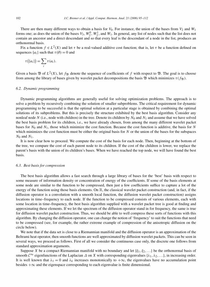
Fig. 1. Diagram for downsampling, orthogonalization and operator compression. (All triangles are commutative by construction.)

Diffusion wavelets allow to lift to these general settings algorithms of multiscale signal processing that are basedon wavelets in R

n, generated by geometric dilation operators.Notwithstanding the level of generality and tunability of the construction of diffusion wavelets, it is well known

that in several applications wavelet bases are not flexible enough and different partitions of the time–frequency planeare useful or even necessary. A library of bases, whose elements are well localized in space and frequency, offer fargreater flexibility, which is needed in several applications, such as compression, denoising, and discrimination amongdifferent classes of signals. The classical wavelet packets of [5] constitute a library of bases, that can be built efficientlyand is organized hierarchically in a dyadic tree of (orthogonal) subspaces. The best basis algorithm of Coifman andco-workers [5,6] and its extensions (see, e.g., [7–9]) take advantage of the hierarchical organization of the library toefficiently search for bases best tailored for any of tasks listed above.

In this paper we present a construction of diffusion wavelet packets, which generalize the classical wavelet packetsand enrich the diffusion scaling function and wavelet bases of [1]. We show that, in many situations arising in ap-plications, efficient algorithms exist for the construction of the packets, for the analysis and synthesis of a functionon the packets and present examples suggesting that the classical best basis algorithms generalize and perform verysatisfactorily the aforementioned tasks.

Material related to this paper, such as examples, and Matlab scripts for their generation, will be made available onthe web page at: http://www.math.yale.edu/~mmm82/diffusionwavelets.html.

2. Diffusion wavelets

We refer the reader to [1] for the construction of diffusion wavelets and for the notation which will be used through-out this paper.

Here we simply recall some basic notation for ease of the reader.We restrict ourselves, for reasons of space, to the finite-dimensional, purely discrete setting. A generalization to

the continuous case is presented in [1].The following definition is from [10]:

Definition 1. Let {T t }t∈[0,+∞) be a family of operators on a measure space (X,μ), each mapping L2(X,μ) into itself.Suppose this family is a semigroup, i.e., T 0 = I and T t1+t2 = T t1T t2 for any t1, t2 ∈ [0,+∞) and limt→0+ T tf = f

in L2(X,μ) for any f ∈ L2(X,μ).Such a semigroup is called a symmetric diffusion semigroup if it satisfies the following:

(i) ‖T t‖p � 1 for every 1 � p � +∞ (contraction property).(ii) Each T t is compact and self-adjoint (symmetry property).

(iii) T t is positive: Tf � 0 for every f � 0 (a.e.) in L2(X) (positivity property).(iv) The semigroup has a generator −Δ, so that

T t = e−tΔ. (2.1)

In the applications we have in mind, (X,μ) is a manifold, or a graph, and in applications to the study and decom-position of singular integrals it can be a space of homogeneous type. The operator T , on a manifold, could be thegenerator of Laplace–Beltrami diffusion semigroup, or, on a graph, I − L, where L is a graph Laplacian. See [1] forexamples and discussion of the above definition.

It is easy to see that the spectrum σT of T is necessarily contained in [0,1].

J.C. Bremer et al. / Appl. Comput. Harmon. Anal. 21 (2006) 95–112 97

L2

P0(T )P1(T )

W0 V0

P0(T 2)P1(T 2)

W1

P0(T )P1(T )

V1

P0(T 4)P1(T 4)

W01 W1

1 W2

P0(T 2)P1(T 2)

V2

W02

P0(T )P1(T )

W12

P0(T )P1(T )

W002 W01

2 W102 W11

2

Fig. 2. Diagram for wavelet packet construction.

The construction of diffusion wavelets is based on the further assumption that the spectrum is concentratedaround 0. This means that high powers of T have low numerical rank and hence can be compressed by projectingon an appropriate subspace.

The idea is then to interpret T as a dilation operator and apply dyadic powers T 2jto pass from scale to scale. At

every stage an orthonormal basis of scaling functions for the numerical range of T 2jis constructed. At each scale the

corresponding dyadic power of T dilates the basis elements and the orthonormalization step of the resulting functionsdownsamples them to an orthonormal basis of the range of that power, which constitutes the next scaling functionspace. Wavelets are obtained by constructing a local orthonormal basis for the orthogonal complement of each scalingspace and the previous one. This is summarized in the diagram in Fig. 1 and the details can be found in [1]. If thesize of an eigenvalue is interpreted as inverse of frequency, diffusion scaling function spaces are “low-frequency”approximation spaces, while diffusion wavelet subspaces are “frequency-band” subspaces at different scales. Theconstruction of diffusion wavelet packets is based upon further subdividing these wavelet subspaces or the associated“frequency-bands.”

3. Diffusion wavelet packets

As it happens in the classical Euclidean setting, the wavelet subspaces Wj can be split into a orthogonal sumsof smaller subspaces. In this way a large family of orthonormal bases, given by the orthogonal direct sum of theorthonormal bases in the smaller subspaces, can be generated. One can then search through these bases fast, becauseof their dyadic tree structure and search for the basis best suited for a specific task [5].

In the classical setting the splitting of a wavelet subspace can be done using the same low-pass and high-pass filtersused to split wavelets and scaling functions spaces. This yields a very symmetric and elegant structure. However, ithas been observed that in some applications the using different filters at different splitting stages yields better results(this are sometimes called nonstationary wavelet packets, see, for example, [11] and references therein).

The construction we are going to present is not as symmetric as the one in the classical, stationary case, sincethe translation at different scales are not linked by simple dilation and downsampling operations, in a way which isinvariant across scales. To introduce the diffusion wavelet packets, we revisit the construction of diffusion wavelets inorder to generalize low-pass and high-pass filters to our setting. With this generalization it will be apparent how theclassical construction can be generalized.

We take the point of view of thinking of low-pass filters as projections onto the numerical range of a (dyadic)power of T and high-pass filters as projections onto the numerical kernel of the same (dyadic) power of T . In theclassical case, T can be thought of as a (usually smooth) multiplier T̂ on the Fourier transform side, with T̂ (0) = 1,d T̂ |ξ=0 = 0, and monotonically decreasing. It is then clear that the classical multiresolution scaling function (“ap-
dξ


proximation”) subspaces Vj can be made correspond to the (numerical) range of T (2j ·), while the multiresolutionwavelet (“detail”) subspaces correspond to the (numerical) kernels of the same power of T .

We proceed analogously in our setting. For any fixed ε > 0, we define the ε-numerical range of an operator A as

ranε(A) = ⟨Av ∈ L2: ‖Av‖2 � ε‖v‖2

⟩.

The definition of ε-numerical kernel is analogous (reverse the inequality!). If A has singular value decomposition

A = UΣV T ,

where U and V are unitary and Σ is diagonal, with positive diagonal entries σ 21 � σ 2

2 � · · · � 0 in nonincreasingorder, we can write

Af =∑

i

σ 2i 〈f, vi〉ui,

where vi are the columns of V and ui the rows of U (these are L2 functions). Then one can define

Aεf =∑σ 2

i >ε

σ 2i 〈f, vi〉ui

and we have

ranε(A) = ran(Aε).

From now on we assume that ε > 0 has been fixed and all the ranges we will consider will be ε-numerical ranges andbe denoted simply by ran. One could choose different values ε at each scale in what follows. We will briefly mentionone such variation below.

For an operator T , we have the chain of subspaces

L2 ⊇ ran(T ) ⊇ ran(T 1+2) ⊇ · · · ⊇ ran

(T 1+2+···+2j ) ⊇ · · ·

which is naturally a multiresolution analysis. We let V−1 = L2 and, for j � 1,

Vj = ran(T 2j −1) = ker

((T ∗)2j −1)⊥

,

so that the chain above reads

L2 = V0 ⊇ V1 ⊇ · · · ⊇ Vj ⊇ · · · .This notation is unfortunately not consistent with the most standard one, where larger j correspond to finer scales, butit seems so natural in our setting that we will adopt it nevertheless.

One then defines, for j � 0, Wj as the orthogonal complement of Vj+1 in Vj , so that

Vj = Vj+1 ⊕⊥ Wj .

In [2] it is shown how orthonormal bases of scaling functions for each subspace Vj can be constructed and it isshown that in the finite-dimensional case, for large classes of operators of interest in applications, an algorithm existsfor constructing them fast, in time n log2(n), where n is the cardinality of the space. The wavelet packets are anextension of this construction, where the spaces Wj are split further into smaller subspaces. Observe that we have, forj � 1,

Wj = ran(T 2j −1) \ ran

(T 2j+1−1) = ker

((T ∗)2j −1)⊥ \ ker

((T ∗)2j+1−1)⊥ (3.1)

and W0 = L2 \ ran(T ). For a fixed j � 1, T l , for any l � 0 is a multiplier on Wj , in the sense that T l(Wj ) ⊆ Wj ,by (3.1). Moreover, if l � 2j , T l(Wj ) = 0. From the point of view of spectral theory, we think of Wj as the Littlewood–

Paley annuli: in the classical Euclidean case these annuli correspond to “frequencies” λ ∈ [2j ,2j+1), in our frameworkthey correspond to the range of eigenvalues λ ∈ [ε(2j+1−1)−1

, ε(2j −1)−1). By the spectral theorem the operator T̂ acts

in the spectral domain by multiplication of functions on its spectrum by λ.This leaves us with 2j powers of T , namely T 2j −1, T 2j −2, . . . , T , T 0 acting on Wj and leaving Wj invariant. Each

of them has a (numerical) range and (numerical) kernel in Wj that gives a natural splitting of Wj . In fact, different


powers can be used at different splitting stages to induce a dyadic hierarchical refinement of Wj as described below.Since we will need a flexible notation for the operation of projecting onto the (numerical) range or (numerical) kernel(which correspond, as noted above) to low- and high-pass filtering, we introduce the following:

Notation 1. For an integer l � 0 we denote its binary representation by b(l). The kth binary digit, starting from themost significative one (so for example k = 0 indicates the leftmost digit), will be denoted by εk(l) ∈ {0,1}.

Notation 2. For an operator A and ε ∈ {0,1}, we let

Pε(A) ={

Pker(A), ε = 0,

Pran(A), ε = 1,(3.2)

where PV , with V close subspace, denotes the orthogonal projection onto V .

We can now define a partition of Wj into smaller subspaces as follows. For j � 1 and s = 0, . . . ,2j − 1, we let

PWsj

= Pεj (s)

(T 20) · · ·Pε1(s)

(T 2j−2)Pε0(s)

(T 2j−1)

, (3.3)

where Wsj is defined as the range of the projection above.

There is an obvious correspondence between the binary expansion of s and the wavelet packet subspace Wsj and a

multiscale family of dyadic subdivisions of the spectrum of T into nested partitions, in bijection with the branches ofthe wavelet packet tree.

Remark 2. When the construction of the wavelet packet tree is carried till a leaf subspace has dimension 1, thenthis one-dimensional subspace is spanned by an eigenfunction of T . In the numerical implementation, this is true toaccuracy, mainly depending on the spectral gaps.

4. Construction of the wavelet packets

The actual algorithm implementing the mathematical construction described in the previous section presents severaldelicate aspects, most of which are common to the construction of diffusion wavelets and are discussed in [1].

The orthogonalization and “downsampling” step is crucial. In the implementation of the algorithm that we usedto create all the examples in this paper we used the algorithm called “modified Gram–Schmidt with mixed L2–L1

pivoting” which was introduced in [1]. In the construction of diffusion wavelet packets there are of course many moreorthogonalization steps, one for each splitting of the wavelet packet subspaces.

A variation on the splitting of a diffusion wavelet packet subspace Wlj , which we adopted in all the examples in

this paper, is to split Wlj into the η-kernel and range of T r , where η was chosen so that these two subspaces would

have the same dimension. This choice of splitting creates more symmetric packet trees.We refer the reader to Appendix A for details on the computational cost of the algorithm.

5. Examples

We consider here two examples of construction of diffusion wavelet packets.The first example is one-dimensional and focuses on an highly anisotropic diffusion operator. It illustrate how

anisotropy can affect the structure of the wavelet packets and the associated time–frequency analysis, in particular therepresentation and compression of functions.

The second example constructs diffusion wavelet packets on the sphere, with respect to (a discrete approximationon scattered points of) the canonical Laplace–Beltrami diffusion. We are considering the sphere, here and in theexamples that follow, only out of simplicity, and ease of visualization. It is clear that our construction can be carriedout on any manifold, for example with respect to the diffusion induced by Laplace–Beltrami operator. In particular,the algorithms used had no knowledge whatsoever about the sphere or its geometry: they are given uniquely the matrixrepresenting the operator (with arbitrary ordering of rows and columns) and generate the full diffusion wavelet packettree automatically.


Fig. 3. Impedance of the anisotropic diffusion operator T : large on one part of the circle and almost 0 on another.

Fig. 4. Some level 7 scaling functions on the anisotropic circle. Notice that the functions exhibit high-frequency behavior in high-impedance regionsand low-frequency behavior in low-impedance regions.

Fig. 5. Wavelet and wavelet packet functions on the anisotropic circle sampled at 256 points.

5.1. Example: anisotropic diffusion on a circle

This example is also considered in [1], from the diffusion wavelets perspective. We start with 256 points equi-spaced on a circle and consider a highly nonuniform impedance on the circle (see Fig. 3). We then consider theoperator T which is the discretization of the nonhomogeneous heat equation on this circle, with this conductance. Thescaling functions, wavelets and wavelet packets exhibit a very nonhomogeneous scaling which is dependent on theconductance around the location of their support (see Figs. 4 and 5).

5.2. Example: Laplace–Beltrami diffusion on a sphere

In this example we consider 2000 points uniformly randomly distributed on the sphere, and the operator T is ob-tained through the Laplace–Beltrami normalization suggested in [3,4]. In Fig. 6 we represent some diffusion waveletsand wavelet packets on the sphere.

6. Best basis algorithms

A (diffusion) wavelet packet decomposition produces a large number of bases of L2(X), each adapted to repre-senting functions with different space and frequency localization properties. We would like to efficiently choose fromthis library of bases the basis which is “most suitable” for a particular task, for example for efficiently representing aparticular function, or maybe for efficiently discriminate between two different classes of functions.

The best basis algorithm of Coifman and Wickerhauser, introduced in [5], is a dynamic programming algorithm forchoosing from a library the basis which minimizes an additive information cost function. Assuming the cost functionhas been well chosen for the particular application (be it compression or denoising or discrimination), the resulting


Fig. 6. Some diffusion wavelets and wavelet packets on the sphere, sampled randomly uniformly at 2000 points.

basis is expected to perform well in the task at hand. For example if the goal is compression, the selected basis will bewell adapted to representing the function; i.e., it will consist of waveforms which closely match the function.

We will now give a brief overview of the best basis algorithm as it applies to diffusion wavelet packets and discusssome of its applications, including compression and denoising.

6.1. Setup

The diffusion wavelet packet decomposition computes bases for a sequence V0, W0, V1, W1, V2, W2, V3, W3, W 02 ,

W 12 , . . . of subspaces of L2(X) which can be arranged in a tree where each space is the direct sum of its children, as

represented in Fig. 2.


There are then many different ways to obtain a basis for V0. For instance, the union of the bases from V2 and W1

forms one; as does the union of the bases V3, W 02 , W 1

2 , and W1. In general, any list of nodes such that the list does notcontain an ancestor and a direct descendant and so that every leaf is the descendant of a node in the list, produces anorthonormal basis.

Fix a function f ∈ L2(X) and let τ be a real-valued additive cost function; that is, let τ be a function defined onsequences {ai} such that τ(∅) = 0 and

τ({ai}

) =∑

i

τ (ai).

Given a basis B of L2(X), let fB denote the sequence of coefficients of f with respect to B. The goal is to choosefrom among the library of bases given by wavelet packet decompositions the basis B which minimizes τ(fB).

6.2. Dynamic programming

Dynamic programming algorithms are generally useful for solving optimization problems. The approach is tosolve a problem by recursively combining the solution of smaller subproblems. The critical requirement for dynamicprogramming to be successful is that the optimal solution at a particular stage is obtained by combining the optimalsolutions of its subproblems. But this is precisely the structure exhibited by the best basis algorithm. Consider anynonleaf node N (i.e., node with children) in the tree. Denote its children by N0 and N1 and assume that we have solvedthe best basis problem for its children, i.e., we have already chosen, from among the many different wavelet packetbases for N0 and N1, those which minimize the cost function. Because the cost function is additive, the basis for N

which minimizes the cost function must be either the original basis for N or the union of the bases for the subspacesN0 and N1.

It is now clear how to proceed. We compute the cost of the basis for each node. Then, beginning at the bottom ofthe tree, we compare the cost of each parent node to its children. If the cost of the children is lower, we replace theparent’s basis with the union of its children’s bases. When we have reached the top node, we will have found the bestbasis.

6.3. Best basis for compression

The best basis algorithm allows a fast search through a large library of bases for the ‘best’ basis with respect tosome measure of information density or concentration of energy of the coefficients. If some of the basis elements atsome node are similar to the function to be compressed, then just a few coefficients suffice to capture a lot of theenergy of the function using those basis elements. On R, the classical wavelet packet construction (and, in fact, if thediffusion operator is a convolution with a smooth local function, the diffusion wavelet packet construction) assignslocations in time–frequency to each node. If the function to be compressed consists of various elements, each withsome location in time–frequency, the best basis algorithm supplied with a wavelet packet tree is good at finding andapproximating these elements. If we let the spectrum of the diffusion operator stand in for frequency, the same is truefor diffusion wavelet packet construction. Thus, we should be able to well compress these sorts of functions with thisalgorithm. By changing the diffusion operator, one can change the notion of ‘frequency’ to suit the functions that needto be compressed (see, for example, the rather extreme example of compression of the anisotropic diffusion on thecircle below).

We note that if the data set is close to a Riemannian manifold and the diffusion operator is an approximation of theBeltrami heat operator, then smooth functions are well approximated by diffusion wavelet packets. This can be seen inseveral ways, we proceed as follows. First of all we consider the continuous case only, the discrete one follows fromstandard approximation arguments.

Suppose X be a compact Riemannian manifold with no boundary and let {ξ1, ξ2, . . .} be the orthonormal basis ofsmooth C∞ eigenfunctions of the Laplacian Δ on X with corresponding eigenvalues {λ1, λ2, . . .}, in increasing order.It is well known that λ1 = 0 and λk increases monotonically to +∞, the eigenvalues have no accumulation pointbesides +∞ and the eigenspace corresponding to each eigenvalue is finite dimensional.


The Sobolev space Hs(X), s ∈ R, is defined as

Hs ={

u ∈D′(X):+∞∑k=1

λsk|ak|2 < +∞

},

with norm

‖u‖Hs =( +∞∑

k=0

(1 + λk)s |ak|2

) 12

.

Here D′(X) is the set of all distributions on X acting on C∞ via the usual pairing.The Sobolev embedding Theorem applies in this context, implying that Hs ⊂ Cl (X) if s > l + dimX

2 . Moreover, theusual duality relation (Hs)∗ = H−s holds.

Consider the heat diffusion semigroup T t = e−tΔ and the associated diffusion wavelet packets. Because of theregularizing properties of T , these packets are smooth functions.

But they have another, more important property: each diffusion wavelet packet is orthogonal to all the eigenfunc-tions of the Laplace operator outside the “frequency band” on which it is supported. This follows immediately fromour construction and it is tautological since being supported in a “frequency band” in this case means exactly beingin the subspace spanned by the eigenfunctions corresponding to eigenvalues in a certain band or, equivalently, beingorthogonal to all the eigenfunctions outside that band.

Then the following rough estimates are routine: suppose the wavelet packet ψ is orthogonal to {ξk}k�K and f ∈ Hs .We have

∣∣〈f,ψ〉∣∣ =∣∣∣∣∣⟨ +∞∑

k=0

〈f, ξk〉ξk,ψ

⟩∣∣∣∣∣ �+∞∑

k=K+1

|ak|∣∣〈ξk,ψ〉∣∣ �

+∞∑k=K+1

|ak|(1 + λk)s2 (1 + λk)

− s2

�( +∞∑

k=K+1

|ak|2(1 + λk)s

) 12( +∞∑

k=K+1

(1 + λk)−s

) 12

� ‖u‖Hs

( +∞∑k=K+1

(1 + λk)−s

) 12

which is decreasing to 0 in K with rate dependent on the speed of convergence of (∑+∞

k=0(1 + λk)−s)

12 . This rate

of convergence improves for increasing s > 0, as expected, depending on the growth rate of the eigenvalues {λk}k .This growth rate, as k → +∞, is controlled uniquely by the dimension of the manifold (by Weyl’s theorem; see, forexample, [12]).

Hence diffusion wavelet packets approximate well smooth (in the Sobolev sense) functions. In fact, they do solocally, since the support of most wavelet packets is small: this is a main difference from the eigenfunction expan-sion. The rate of convergence of a diffusion wavelet (packet) expansion will depend on the local smoothness of thefunctions, while the rate of convergence of the Laplace eigenfunction expansion is affected by the global smoothness.This is of course completely analogous to what happens even in one dimension, on the real line, where Fourier seriescorrespond to (is!) the expansion on Laplace eigenfunctions and classical wavelet analysis corresponds to diffusionwavelet analysis.

We also want to remark that our diffusion may be chosen not to depend only on geometrical properties of the space:the diffusion operator T can have anisotropies on its own, not dictated by the geometry of the space (e.g., curvature,like the Laplace–Beltrami operator). If we define smoothness spaces as spaces of functions well approximated bydiffusion wavelet packets associated to T , these functions spaces will depend on T and on its anisotropies. We willsee a simple but yet remarkable example of the anisotropy of the spaces well approximated by diffusion waveletpackets in the compression example on the anisotropic circle presented below. The study of these spaces is mostnaturally carried out in the biorthogonal setting [13].

6.4. Best basis for denoising

If we know that a class of functions is well compressed by wavelet packets, then by thresholding the coefficients,we expect to be able to denoise functions from the class (assuming, of course, that the ‘noise’ is not well compressed


by wavelet packets). Efficient and asymptotically optimal denoising algorithms for denoising have been studied byDonoho and Johnstone [14].

6.5. Local discriminant bases

The best basis algorithm can also be used to solve classification problems in function spaces on a data set or amanifold, using the Local Discriminant Basis algorithm of [7–9]. Instead of using entropy (or some other measureof description efficiency) to choose nodes, we use an additive cost function that measures how well a particular basisnode discriminates between the classes. More specifically, we assume we have training functions fnm, grouped intoM classes Cm. For each basis function w, we find

ΓCm(w) =|Cm|∑n=1

∣∣〈w,fnm〉∣∣2/|Cm|∑

n=1

|fnm|2

and then apply a discriminant measure D to the sequence ΓCm(w), obtaining

Γ (w) =M−1∑i=1

M∑j=i+1

D(ΓCi

(w) − ΓCj(w)

)as the cost of a basis function w. The discriminant measure is chosen to reward large differences in correlationsbetween classes; some popular choices include |x − y|p , or symmetric cross entropy,

D(x,y) = x logx/y + y logy/x.

After we have calculated the costs of the individual w’s, in order to calculate the cost of a node we sum the costs of thebasis elements in that node. Then we run the ‘worst’ basis algorithm, finding the basis with the highest cost. Finally,the most discriminating few basis vectors are passed into a regression scheme, usually allowing a large reduction inthe dimensionality of the problem and more robust statistical estimation. Note that each step in this process is fast oncewe have the coefficients for the training data (with constants depending linearly on the number of training functionsand quadratically in the number of classes) and that finding the coefficients for the training data is fast because of theproperties of the diffusion wavelet transform.

This algorithm works when we are able to encode information about the geometry of the dataset in the diffusionoperator and our function classes respect that information. For example, if the data were a discretization of a manifoldin some Euclidean space (or if it lay close to a manifold), we could take the heat kernel of the manifold as our operator,calculated from the points as in [3,4]. If the classes of functions to be distinguished are differentiated by the location oftheir energy, or otherwise differentiated by the geometry of the manifold, then the algorithm will find and utilize thisinformation. We can expect even better success if the functions are also differentiated by their behavior in ‘frequency,’i.e., the function classes are localized in different regions of the spectrum of the Laplacian. Note that the only part ofthe algorithm operating on the original points of the dataset is the nearest neighbor search in the construction of thediffusion kernel. This has the important consequence of desensitizing the algorithm to the ambient space of the data.It also suggests that some classification problems that are not presented with an obvious geometric structure might begiven one by finding an appropriate diffusion.

7. Examples

7.1. Compression on the anisotropic circle

We choose 256 equally spaced points on the circle and construct an anisotropic diffusion operator T with im-pedance as shown in Fig. 7, see also [1]. We expect that the wavelet packet bases generated using T will be welladapted to representing high-frequency details where the impedance of T is large and slowly varying features whereit is low.

To test this thesis we construct a function F with these properties. We find the coefficients of F and its reflectionin their best diffusion wavelet packet bases using the l1 norm as a cost function. Since the reflection has the opposite


Fig. 7. The function F (on the left) and its reflection.

Fig. 8. Comparison of the magnitude first 50 coefficients of F and its reflection in their best wavelet packet bases.

Fig. 9. Two different views of the function F on the sphere.

structure, that is, its high-frequency component is aligned with the low-impedance and its low frequency componentis aligned with high impedance, we expect the representation of F to be more efficient than that of its reflection.

This is indeed what happens; Fig. 8 compares the magnitude of the resulting coefficients of F and its reflection.

7.2. Compression on the sphere, I

Our data set consists of 2000 random points uniformly distributed on the unit sphere and our diffusion is theoperator T with kernel K(x,y) = χ|x−y|<ε . We construct a function F consisting of a smooth slowly oscillatingfunction and the characteristic function of a set, as represented in Fig. 9 (two different views).

We find the best diffusion wavelet packet basis using the l1 norms of coefficients as a cost function. The coefficientsof F in this basis, in the diffusion wavelet basis, and in the eigenfunction basis are compared in Fig. 10. Since the


Fig. 10. Log plot of the decay of the magnitude of coefficients, in the best basis, diffusion wavelets and eigenfunctions. The coefficients on thediffusion wavelet basis have essentially the same decay as the ones on the best basis.

Fig. 11. Left: reconstruction of the function F with top 50 best basis packets. Right: reconstruction with top 200 eigenfunctions of the Bel-trami–Laplacian operator.

function F has sharp discontinuities, we expect the best wavelet packet basis to perform better than the basis ofeigenfunctions of the Laplace–Beltrami operator ΔB . In Fig. 11, we see a comparison of the coefficients in the waveletpacket best basis and eigenfunction basis.

The reconstruction of F from the first 200 coefficients of the best basis is shown in Fig. 11. Notice that both thesmoothly varying and the sharp features of F are reconstructed (albeit imperfectly).

The eigenfunctions we used for comparison are computed in the following way: we consider 10,000 pointsuniformly distributed on the sphere, that include the 2000 points considered above, and we consider the diffusionoperator Δ obtaining by approximating the continuous Laplace–Beltrami operator ΔB as suggested in [3,4]. We com-pute the eigenfunctions of this operator and then restrict them to the 2000 points considered in the example above.The restricted eigenfunctions are not orthonormal and we orthonormalize them proceeding from low-frequency tohigh-frequency. The reason for this procedure is that the operator Δ̃ we obtain if we try to approximate to ΔB usingonly 2000 points is quite far from the true ΔB (see the estimates in [3]), because of the nonuniformity of the pointson the sphere. As a result, the eigenfunctions of Δ̃ are terrible approximations of the true eigenfunctions of ΔB , inparticular of course for high-frequency eigenfunctions, which are important in our problem because of their role inapproximating discontinuities. In fact, the high-frequency eigenfunctions of Δ̃ seem very well-localized (!), insteadof being global spherical prolates and do a much better job than the eigenfunctions of ΔB .

7.3. Compression on the sphere, II

The set of points and the corresponding diffusion operator are as before, and the function F we consider is shownin Fig. 12.

Once again we use the l1 norm as a cost function. The coefficients of F in this basis, in the diffusion wavelet basis,and in the eigenfunction basis are compared in Fig. 13.


Fig. 12. Two different views of the function F on the sphere.

Fig. 13. Coefficients of the expansion of F on the best diffusion wavelet packet basis, diffusion wavelets and eigenfunctions.

Fig. 14. Left: reconstruction of the function F from 200 best basis diffusion wavelet packet coefficients. Right: reconstruction from top 200eigenfunctions.

The reconstruction of F from the first 200 coefficients of the best basis is shown in Fig. 14. Since the eigenfunctionsare not localized in space, the reconstruction of F from them relies on delicate cancellations. This requires a largenumber of coefficients to even begin to reconstruct the major features of the function F . The result of reconstructingF from 200 eigenfunctions is seen in Fig. 14.

7.4. De-noising on the sphere

Now we test the best wavelet packet denoising technique of Donoho and Johnstone [14] on the 2000 point sphere.We begin with a function G which is a periodic wave on the sphere; two views of G are given in Fig. 15. We add0.25η to the function G, where η is Gaussian white noise of mean 0 and variance 1: we represent this function inFig. 16.


Fig. 15. Two views of G.

Fig. 16. Left: G with noise; right: G denoised.

The best diffusion wavelet basis is found using the cost function described in [5,6]. The first 40 coefficients of G

in the best basis are used to reconstruct the function (see Fig. 16). The signal-to-noise ratio of the function G withadded noise is 6.49, the signal-to-noise ration of the denoised function is 10.8.

7.5. Local discriminant bases on a space curve

To illustrate the LDB algorithm using diffusion wavelets, we adapt an example from Naoki Saito’s thesis [7]. Forour data set, we choose 1024 random sample points on the curve

x(t) = (4 + sin 6πt)(cos 2πt), y(t) = (4 + sin 6πt)(sin 2πt), z(t) = cos 6πt,

with a uniform distribution. We will attempt to distinguish between three classes of synthetic functions on this dataset. Let s be arclength, the length of the curve be L, a and c be uniform random variables with ranges [L/8,L/4]


Fig. 17. Left to right, a realization of a function from class 1, 2, 3.

and [L/4,3L/4], respectively, let b = a + c, and η be a standard normal variable. Then class 1 functions are of theform (6 + η)χa,b(s), class 2 functions are of the form (6 + η)χa,b(s − a)/(b − a), and class 3 functions are of theform (6 + η)χa,b(b − s)/(b − a). To all three classes of functions, we add standard normal white Gaussian noise. Werefer the reader to Fig. 17 for a realization of the three random variables. Note that though we define the functions bythe natural parameter of the curve, we do not give the algorithm the functions in that parameter; rather, the points aregiven in the order they were sampled. The algorithm has to discover the parameter.

A wavelet packet tree is generated from Gaussian kernel normalized as in [3,4] to approximate the Laplace–Beltrami operator on the curve (which is standard one dimensional diffusion with respect to arclength), the ‘worst’basis is chosen using symmetric cross entropy as a discriminant measure and we select the 30 costliest basis vectorsand run a CART (Classification And Regression Tree) to do the actual classification. A CART tested on the set of 999functions in the original 1024 coordinates has a test error of 0.137. Using the full LDB coordinates brings the testerror down to 0.112. The test error using only the 30 top LDB coordinates is 0.059. In this example, an inspection ofthe classification tree and chosen basis functions shows that the algorithm works because the basis functions respectthe geometry of the data set, and the function classes are determined by where on the data set they have more energy.

7.6. Local discriminant bases on the sphere, I

We now give two examples using LDB to distinguish between classes of synthetic functions on the uniformlysampled 2000 point sphere from above. As above, we use the normalized χ operator to generate the packet tree.

For the first example, we fix a point v and then let w be the random perturbation of v given by w = (v+0.1η)/‖v+0.1η‖, where η is a standard normal Gaussian in R

3. We center a ripple of the form

f (x) = χD cos(C cos−1〈w,x〉)

about w and depending on the class, C is chosen so there are one or two complete radial oscillations. Now we place 5more ripples of random type (one or two oscillations) in random nonoverlapping locations around the sphere. Finally,we add 0.2 white Gaussian noise. See Fig. 18.

A CART run on the delta basis of the original data set has a test error of 0.175 with 300 training functions and 1000test functions. If we use the symmetric cross entropy to find the top 20 LDB coordinates, we can reduce the test errorto 0.035. Note for comparison that a CART using the first 300 eigenfunctions of our χ operator as coordinates hasa 0.31 test error. Observe that the eigenfunctions of χ are quite different from the eigenfunctions of the continuousLaplace–Beltrami operator ΔB on the sphere. In particular, the high-frequency eigenfunctions of χ are nicely localizedand oscillating and in general are much better suited to these discrimination tasks than good approximations to theeigenfunctions of ΔB . This remark applies to the following example as well.

7.7. Local discriminant bases on the sphere, II

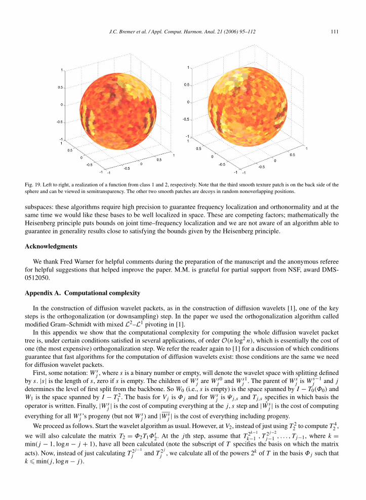
For our second example, we place three equally spaced points along a random (but fixed) equator of the circle. Asabove, we then perturb each point by adding 0.1η and renormalizing, where η is a standard normal Gaussian. Now wecenter a patch of texture of the form

f (x) = χD sin(20 cos−1〈v, x〉)

at each perturbed point, where v is either in the plane of the equator or perpendicular to it, depending on the class ofthe function. For class 1 functions, the textures on all three patches are the same, with equal probability that the ridges


Fig. 18. Left to right, a realization of a function from class 1 and 2, top and bottom are two views of the same realization, from two antipodal pointsof view.

on the patches are either parallel or perpendicular to the chosen equator. For class 2 functions, after choosing theorientation of the texture patches, we randomly select one patch, and orient it the other way. We add some truncatedGaussian bumps at random locations near the poles as decoys, and as usual, we add 0.2 white Gaussian noise. SeeFig. 19.

At this point, a CART run on the original data with 300 training functions has a test error (with 1000 test functions)of 0.481, that is, it essentially saw no difference between the classes. Building a packet tree with the normalized χ

diffusion from above and picking the top 40 LDB vectors using the l2 discriminant measure yields a test error rateof 0.125. In this example using the first 300 eigenfunctions of the χ operator as coordinates does almost as well,leading to a test error of 0.181.

8. Conclusions

Diffusion wavelet packets allow for flexible multiscale space–frequency analysis for functions on manifolds andgraphs. The associated best basis algorithms allow for efficient search through a library of packets, for various signalprocessing tasks.

Several generalizations of the construction presented here are possible: for example different choice of splittingfor the wavelet packet subspaces, different frequency filters (instead of just powers of the diffusion operator). Thedeepest problems are related to the numerical algorithms used for the construction of the orthonormal bases in these


Fig. 19. Left to right, a realization of a function from class 1 and 2, respectively. Note that the third smooth texture patch is on the back side of thesphere and can be viewed in semitransparency. The other two smooth patches are decoys in random nonoverlapping positions.

subspaces: these algorithms require high precision to guarantee frequency localization and orthonormality and at thesame time we would like these bases to be well localized in space. These are competing factors; mathematically theHeisenberg principle puts bounds on joint time–frequency localization and we are not aware of an algorithm able toguarantee in generality results close to satisfying the bounds given by the Heisenberg principle.

Acknowledgments

We thank Fred Warner for helpful comments during the preparation of the manuscript and the anonymous refereefor helpful suggestions that helped improve the paper. M.M. is grateful for partial support from NSF, award DMS-0512050.

Appendix A. Computational complexity

In the construction of diffusion wavelet packets, as in the construction of diffusion wavelets [1], one of the keysteps is the orthogonalization (or downsampling) step. In the paper we used the orthogonalization algorithm calledmodified Gram–Schmidt with mixed L2–L1 pivoting in [1].

In this appendix we show that the computational complexity for computing the whole diffusion wavelet packettree is, under certain conditions satisfied in several applications, of order O(n log2 n), which is essentially the cost ofone (the most expensive) orthogonalization step. We refer the reader again to [1] for a discussion of which conditionsguarantee that fast algorithms for the computation of diffusion wavelets exist: those conditions are the same we needfor diffusion wavelet packets.

First, some notation: Wsj , where s is a binary number or empty, will denote the wavelet space with splitting defined

by s. |s| is the length of s, zero if s is empty. The children of Wsj are Ws0

j and Ws1j . The parent of Ws

j is Ws−1j and j

determines the level of first split from the backbone. So W0 (i.e., s is empty) is the space spanned by I − T0(Φ0) andW1 is the space spanned by I − T 2

1 . The basis for Vj is Φj and for Wsj is Ψj,s and Tj,s specifies in which basis the

operator is written. Finally, |Wsj | is the cost of computing everything at the j, s step and |W̊ s

j | is the cost of computing

everything for all Wsj ’s progeny (but not Ws

j ) and |Wsj | is the cost of everything including progeny.

We proceed as follows. Start the wavelet algorithm as usual. However, at V2, instead of just using T 22 to compute T 4

2 ,

we will also calculate the matrix T2 = Φ2T1Φt2. At the j th step, assume that T 2k−1

k−1 , T 2j−2

j−1 , . . . , Tj−1, where k =min(j − 1, logn − j + 1), have all been calculated (note the subscript of T specifies the basis on which the matrixacts). Now, instead of just calculating T 2j−1

j and T 2j

j , we calculate all of the powers 2k of T in the basis Φj such thatk � min(j, logn − j).


So at this point we will start to assume all of our matrix multiplications and all calls to the orthonormalizationalgorithm are at worst O(n log2 n). With these assumptions and the assumption that each Vj is half the size of the pre-vious one, we can count the operations on the “backbone” of the packet tree. At each Vj , we have to compute at mostC(j + 2) (and actually just C(min(j, logn − j) + 2)) matrix multiplications or calls to the orthonormalization algo-rithm to get all the necessary operators (the +2 is for orthonormalization and for applying the operator, the C becausepushing each operator forward takes two sparse matrix multiplications). Each one takes at most |Φj−1| log2 |Φj−1|operations. So in total, since the series

∑ j

22j is summable, O(n log2 n) to do the backbone.Now we should calculate the cost of the wavelet branches of the tree.We use the same philosophy as above for generating the wavelet spaces—before proceeding to find the bases of

the children of a space, we record all operators that will be used by that space’s children. Note that this keeps us fromhaving to walk all the way back up the tree, and also, that since the basis transformations should be sparse, at leastone matrix in all the multiplications should be sparse. So the first claim is that |W̊ s

j | � C2(j + 2)(j − |s| − 1)|Ψ sj |2.

This can be seen by induction on j − |s| − 1 (i.e., we induct up the tree). If j − |s| − 1 = 1, since we only usepositive powers of the operator, there is only one split possible. For simplicity, to estimate the operation count, we willcalculate all j powers of the operator at each node of the j th branch (instead of j − |s| − 1 powers.

We need to apply Tj,s and I −Tj,s to Ψj,s and orthonormalize the resulting sets of vectors. This costs 2C(j + 2)×|Ψj,s |2 operations, as desired.

Now assume the statement is true for j − |s| − 1 = k. We need to calculate |W̊ sj |, where j − |s| − 1 = k + 1.

As above, |Ws0j | and |Ws1

j | are each C(j + 2)|Ψ sj |2. Also, since Ψ s0

j and Ψ s1j split Ws

j , |Ψ s0j | + |Ψ s1

j | = |Ψ sj |. Set

|Ψ s0j | = α. Then∣∣W̊ s

j

∣∣ = ∣∣Ws0j

∣∣ + ∣∣Ws1j

∣∣ + ∣∣W̊ s0j

∣∣ + ∣∣W̊ s1j

∣∣= C(j + 2)

∣∣Ψ sj

∣∣2 + C(j + 2)(j − |s| − 2

)α2

∣∣Ψ sj

∣∣2 + C(j + 2)(j − |s| − 2

)(1 − α)2

∣∣Ψ sj

∣∣2

� 2C(j + 2)∣∣Ψ s

j

∣∣2 + 2C(j + 2)(j − |s| − 2

)∣∣Ψ sj

∣∣2 = 2C(j + 2)(j − |s| − 1

)∣∣Ψ sj

∣∣2.

Now to get from Vj−1 to Wj takes C(j + 2)|Φj1 |2 operations and |Ψj | = n/2j . At this point we have used theassumption that each application of M halves the space—one might worry about the size of the wavelet spaces beingto large if it does more than half, but then the wavelet spaces could be bounded by the V one higher on the backbone.

Then the cost |Wj | � 2C(j+2)jn2

22j . The series∑ j2

22j is summable, so the entire algorithm is O(n log2 n).

References

[1] R.R. Coifman, M. Maggioni, Diffusion wavelets, Appl. Comput. Harmon. Anal. 21 (1) (2006) 54–95.[2] R.R. Coifman, M. Maggioni, Multiresolution analysis associated to diffusion semigroups: Construction and fast algorithms, Technical report

YALE/DCS/TR-1289, Yale University, 2004.[3] S. Lafon, Diffusion maps and geometric harmonics, Ph.D. thesis, Yale University, 2004.[4] R.R. Coifman, S. Lafon, A. Lee, M. Maggioni, B. Nadler, F. Warner, S. Zucker, Geometric diffusions as a tool for harmonic analysis and

structure definition of data. Part I. Diffusion maps, Proc. Natl. Acad. Sci. 102 (2005) 7426–7431.[5] R.R. Coifman, M.V. Wickerhauser, Entropy-based algorithms for best basis selection, IEEE Trans. Inform. Theory 38 (2) (1992) 713–718.[6] R.R. Coifman, Y. Meyer, S. Quake, M.V. Wickerhauser, Signal processing and compression with wavelet packets, in: Progress in Wavelet

Analysis and Applications, Frontières, Gif, 1993, pp. 77–93.[7] N. Saito, Local feature extraction and its applications using a library of bases, Ph.D. thesis, Yale Mathematics Department, 1994.[8] R.R. Coifman, N. Saito, Constructions of local orthonormal bases for classification and regression, C. R. Acad. Sci. Paris Sér. I 319 (1994)

191–196.[9] R.R. Coifman, N. Saito, F.B. Geshwind, F. Warner, Discriminant feature extraction using empirical probability density estimation and a local

basis library, Pattern Recogn. 35 (2002) 2841–2852.[10] E. Stein, Topics in Harmonic Analysis Related to the Littlewood–Paley Theory, Princeton Univ. Press, Princeton, NJ, 1970.[11] M. Nielsen, Highly nonstationary wavelet packets, Appl. Comput. Harmon. Anal. 12 (2) (2002) 209–229.[12] S. Rosenberg, The Laplacian on a Riemannian Manifold, London Mathematical Society Student Texts, vol. 31, Cambridge Univ. Press, New

York, 1997.[13] M. Maggioni, J.C. Bremer Jr., R.R. Coifman, A.D. Szlam, Biorthogonal diffusion wavelets for multiscale representations on manifolds and

graphs, in: Wavelet XI, in: Proc. SPIE, vol. 5914, 2005, 5914D.[14] D.L. Donoho, I. Johnstone, Ideal denoising in an orthonormal basis chosen from a library of bases, Technical report, Stanford University,

1994.

Diffusion wavelet packets - UC Davis Mathematicsbremer/papers/wavelets.pdfDiffusion wavelet packets...

Documents

Transcript of Diffusion wavelet packets - UC Davis Mathematicsbremer/papers/wavelets.pdfDiffusion wavelet packets...