NORTH ATLANTIC TREATY ORGANISATION

RESEARCH AND TECHNOLOGYORGANISATION

AC/323(SCI-135)TP/189 www.rto.nato.int

RTO AGARDograph 160 Flight Test Instrumentation Series – Volume 21

SCI-135

Differential Global Positioning System (DGPS) for Flight Testing

(Global Positioning System Différentiel (DGPS) pour les essais en vol)

This AGARDograph has been sponsored by SCI-135, the

Flight Test Technology Task Group of the Systems

Concepts and Integration Panel (SCI) of RTO.

Published October 2008

Distribution and Availability on Back Cover

NORTH ATLANTIC TREATY ORGANISATION

RESEARCH AND TECHNOLOGYORGANISATION

AC/323(SCI-135)TP/189 www.rto.nato.int

RTO AGARDograph 160 Flight Test Instrumentation Series – Volume 21

SCI-135

Differential Global Positioning System (DGPS) for Flight Testing

(Global Positioning System Différentiel (DGPS) pour les essais en vol)

This AGARDograph has been sponsored by SCI-135, the

Flight Test Technology Task Group of the Systems

Concepts and Integration Panel (SCI) of RTO.

Authored by

Maj. Roberto Sabatini, Ph.D. Aeronautica Militare

Reparto Sperimentale di Volo Aeroporto Pratica di Mare

00040 – Pomezia (RM) Italy

Prof. Giovanni B. Palmerini, Ph.D. Università degli Studi “La Sapienza” di Roma

Scuola di Ingegneria Aerospaziale Via Eudessiana, 16

00184 – Roma Italy

ii RTO-AG-160-V21

The Research and Technology Organisation (RTO) of NATO

RTO is the single focus in NATO for Defence Research and Technology activities. Its mission is to conduct and promote co-operative research and information exchange. The objective is to support the development and effective use of national defence research and technology and to meet the military needs of the Alliance, to maintain a technological lead, and to provide advice to NATO and national decision makers. The RTO performs its mission with the support of an extensive network of national experts. It also ensures effective co-ordination with other NATO bodies involved in R&T activities.

RTO reports both to the Military Committee of NATO and to the Conference of National Armament Directors. It comprises a Research and Technology Board (RTB) as the highest level of national representation and the Research and Technology Agency (RTA), a dedicated staff with its headquarters in Neuilly, near Paris, France. In order to facilitate contacts with the military users and other NATO activities, a small part of the RTA staff is located in NATO Headquarters in Brussels. The Brussels staff also co-ordinates RTO’s co-operation with nations in Middle and Eastern Europe, to which RTO attaches particular importance especially as working together in the field of research is one of the more promising areas of co-operation.

The total spectrum of R&T activities is covered by the following 7 bodies: • AVT Applied Vehicle Technology Panel • HFM Human Factors and Medicine Panel • IST Information Systems Technology Panel • NMSG NATO Modelling and Simulation Group • SAS System Analysis and Studies Panel • SCI Systems Concepts and Integration Panel

• SET Sensors and Electronics Technology Panel

These bodies are made up of national representatives as well as generally recognised ‘world class’ scientists. They also provide a communication link to military users and other NATO bodies. RTO’s scientific and technological work is carried out by Technical Teams, created for specific activities and with a specific duration. Such Technical Teams can organise workshops, symposia, field trials, lecture series and training courses. An important function of these Technical Teams is to ensure the continuity of the expert networks.

RTO builds upon earlier co-operation in defence research and technology as set-up under the Advisory Group for Aerospace Research and Development (AGARD) and the Defence Research Group (DRG). AGARD and the DRG share common roots in that they were both established at the initiative of Dr Theodore von Kármán, a leading aerospace scientist, who early on recognised the importance of scientific support for the Allied Armed Forces. RTO is capitalising on these common roots in order to provide the Alliance and the NATO nations with a strong scientific and technological basis that will guarantee a solid base for the future.

The content of this publication has been reproduced directly from material supplied by RTO or the authors.

Published October 2008

Copyright © RTO/NATO 2008 All Rights Reserved

ISBN 978-92-837-0041-8

Single copies of this publication or of a part of it may be made for individual use only. The approval of the RTA Information Management Systems Branch is required for more than one copy to be made or an extract included in another publication. Requests to do so should be sent to the address on the back cover.

RTO-AG-160-V21 iii

AGARDograph Series 160 and 300 Soon after its founding in 1952, the Advisory Group for Aerospace Research and Development (AGARD) recognized the need for a comprehensive publication on Flight Test Techniques and the associated instrumentation. Under the direction of the Flight Test Panel (later the Flight Vehicle Integration Panel, or FVP) a Flight Test Manual was published in the years 1954 to 1956. This original manual was prepared as four volumes: 1. Performance, 2. Stability and Control, 3. Instrumentation Catalog, and 4. Instrumentation Systems.

As a result of the advances in the field of flight test instrumentation, the Flight Test Instrumentation Group was formed in 1968 to update Volumes 3 and 4 of the Flight Test Manual by publication of the Flight Test Instrumentation Series, AGARDograph 160. In its published volumes AGARDograph 160 has covered recent developments in flight test instrumentation.

In 1978, it was decided that further specialist monographs should be published covering aspects of Volumes 1 and 2 of the original Flight Test Manual, including the flight testing of aircraft systems. In March 1981, the Flight Test Techniques Group (FTTG) was established to carry out this task and to continue the task of producing volumes in the Flight Test Instrumentation Series. The monographs of this new series (with the exception of AG237 which was separately numbered) are being published as individually numbered volumes in AGARDograph 300. In 1993, the Flight Test Techniques Group was transformed into the Flight Test Editorial Committee (FTEC), thereby better reflecting its actual status within AGARD. Fortunately, the work on volumes could continue without being affected by this change.

An Annex at the end of each volume in both the AGARDograph 160 and AGARDograph 300 series lists the volumes that have been published in the Flight Test Instrumentation Series (AG 160) and the Flight Test Techniques Series (AG 300) plus the volumes that were in preparation at that time. Annex B of this paper reproduces current such listings.

iv RTO-AG-160-V21

Differential Global Positioning System (DGPS) for Flight Testing (RTO AG-160 Vol. 21 / SCI-135)

Executive Summary Historically, test ranges have provided accurate time and space position information (TSPI) by using laser tracking systems, kinetheodolite systems, tracking radars, and ground-based radio positioning systems. These systems have a variety of limitations. In general, they provide a TSPI solution based on measurements relative to large and costly fixed ground stations. Weather has an adverse effect on many of these systems, and all of them are limited to minimum altitudes or confined geographic regions.

The Global Positioning System (GPS) provides a cost-effective capability that overcomes nearly all the limitations of existing TSPI sources. GPS is a passive system using satellites, which provides universal and accurate source of real-time position, and timing data to correlate mission events. The coverage area is unbounded and the number of users is unlimited. The use of land-based differential GPS (DGPS) reference stations improves accuracy to about one meter for relatively stationary platforms, and to a few meters for high performance tactical aircraft. Further accuracy enhancement can be obtained by using GPS carrier phase measurements, either in post-processing or in real-time. Accuracy does not degrade at low altitudes above the earth’s surface, and loss of navigation solution does not occur as long as the antenna has an open view of the sky. Therefore, it was important to undertake a study in order to investigate the range of possible applications of DGPS in the flight test environment, taking also into account possible integration (in real-time and in post-processing) with other systems.

In this AGARDograph, the potential of DGPS as a positioning datum for flight test applications is deeply discussed. Current technology status and future trends are investigated in order to identify optimal system architectures for both the on-board and ground station components, and to define optimal strategies for DGPS data gathering during various flight testing tasks. Limitations of DGPS techniques are deeply analyzed, and various possible integration schemes with other sensors are considered. Finally, the architecture of an integrated position reference system suitable for flight test applications is identified.

The purpose of this AGARDograph is to provide comprehensive guidance on assessing the need for and determining the characteristics of DGPS based position reference systems for flight test activities. The specific goals are to make available to the NATO flight test community the best practices and advice for DGPS based systems architecture definition and equipment selection. A variety of flight test applications are examined and both real-time and post-mission DGPS data requirements are outlined. Particularly, DGPS accuracy, continuity and integrity issues are considered, and possible improvements achievable by means of signal augmentation strategies are identified. Possible architectures for integrating DGPS with other airborne sensors (e.g., INS, Radalt) are presented, with particular emphasis on current and likely future data fusion algorithms. Particular attention is devoted to simulation analysis in support of flight test activities with DGPS. Finally, an outline of current research perspectives in the field of DGPS technology is given.

RTO-AG-160-V21 v

Global Positioning System Différentiel (DGPS) pour les essais en vol

(RTO AG-160 Vol. 21 / SCI-135)

Synthèse Historiquement, l’étendue des tests a fourni une information exacte sur la position dans le temps et dans l’espace (TSPI) en utilisant des systèmes de poursuite à laser, des systèmes cinéthéodolites, des radars de poursuite, et des systèmes de positionnement radio au sol. Ces systèmes ont un ensemble de limitations. En général, ils fournissent une solution TSPI basée sur des mesures données par des stations sol fixes importantes et coûteuses. Le temps a un effet défavorable sur la plupart de ces systèmes qui sont tous limités à une altitude minimum et à des régions géographiquement restreintes.

Le Global Positioning System (GPS) fournit des moyens bons marchés qui surmontent à peu près toutes les limitations des sources TSPI existantes. Le GPS est un système passif par satellites qui fournit une source universelle et précise de la position en temps réel, il fournit aussi des données en temps sur la poursuite de la mission. La couverture dans l’espace est sans borne et le nombre d’utilisateurs est illimité. L’utilisation de stations au sol de référence de différentiels GPS (DGPS) augmente la précision jusqu’à environ un mètre pour les plateformes relativement stationnaires et de quelques mètres pour les avions tactiques hautement performants. Un accroissement supplémentaire de la précision peut être obtenu en utilisant les mesures de phase de transport, soit dans les opérations à venir, soit en temps réel. La précision ne se dégrade pas à basse altitude, une perte de navigation ne peut survenir tant que l’antenne a une vue dégagée du ciel. De ce fait, il était important d’entreprendre une étude pour enquêter sur l’étendue des applications possibles du DGPS pour les essais en vol, en tenant compte aussi de l’intégration possible des autres systèmes (en temps réel et à venir).

Dans cette AGARDographie, les données du DGPS sur la position des essais en vol, sont sérieusement examinées. L’état de la technologie actuelle et les tendances futures sont étudiés de façon à identifier les meilleurs systèmes d’architectures à la fois sur le plan des équipements à bord et au sol, et aussi sur les stratégies optimales pour récupérer les données DGPS lors des différentes tâches pendant les essais en vol. Les limitations des techniques DGPS sont profondément analysées et les différents schémas possibles d’intégration avec les autres détecteurs sont étudiés. En définitif, l’architecture d’un système de référence des positions intégrées adaptable aux essais en vol, a été identifié.

L’AGARDographie veut fournir des conseils d’ensemble sur l’estimation des besoins et déterminer les caractéristiques de base des systèmes de référence de position DGPS pour les essais en vol. Le but spécifique est de mettre à la disposition de la communauté des essais en vol de l’OTAN des pratiques et des conseils afin qu’elle choisisse l’équipement et la définition architecturale des systèmes DGPS. Un ensemble d’applications pour les essais en vol est étudié et les données indispensables du DGPS en temps réel et après mission sont répertoriées. En particulier, les questions sur la précision, la continuité et l’intégrité du DGPS sont déterminées et des améliorations réalisables, par l’accroissement de puissance des signaux, sont identifiées. De possibles architectures intégrant d’autres détecteurs (ex.: INS, Radalt) sont présentées, en insistant sur les algorithmes de données intégrant l’actuel et le futur. L’analyse de simulation liée aux essais en vol est particulièrement étudiée avec le DGPS. Enfin, il en ressort une vue d’ensemble sur les perspectives de recherches actuelles dans le domaine de la technologie DGPS.

vi RTO-AG-160-V21

Acknowledgements We would like to express our gratitude to Prof. Ugo Ponzi and Prof. Filippo Graziani for strongly supporting this project since its earliest stages.

We would also like to thank Prof. Carlo Buongiorno, Prof. Paolo Teofilatto, Prof. Fabio Santoni, and all other staff members of the School of Aerospace Engineering in Rome University “La Sapienza”.

Special thanks go to Prof. Vidal Ashkenazi, Prof. Alan Dodson and Prof. Terry Moore from Nottingham University, and to Dr. Mark Richardson from Cranfield University, for their valuable guidance and support.

Great thanks go to the Italian Air Force Flight Test Centre Commander and Technical Director for giving us the opportunity of working on this project.

Many thanks go to Sam Storm Van Leeuwen from NLR and to the personnel of ALENIA AEROSPAZIO, AERMACCHI, ASHTECH/THALES and TRIMBLE for their valuable technical advice and support.

RTO-AG-160-V21 vii

Table of Contents

Page

AGARDograph Series 160 and 300 iii

Executive Summary iv

Synthèse v

Acknowledgements vi

List of Figures xii

List of Tables xv

List of Acronyms xvi

Preface xix

Chapter 1 – Differential GPS 1-1 1.1 Introduction 1-1 1.2 DGPS Concept 1-1 1.3 DGPS Implementation Types 1-3

1.3.1 Ranging-Code Differential GPS 1-3 1.3.1.1 Single Difference Between Receivers 1-4 1.3.1.2 Double Difference Observable 1-5

1.3.2 Carrier-Phase Differential GPS 1-5 1.3.2.1 Single Difference Observable 1-6 1.3.2.2 Double Difference 1-6

1.3.3 DGPS Datalink Implementations 1-7 1.3.4 Local Area and Wide Area DGPS 1-8

1.4 DGPS Accuracy 1-9 1.5 DGPS Error Sources 1-10 1.6 Integrity Issues for Aircraft Navigation 1-12 1.7 DGPS Augmentation Systems 1-13 1.8 References 1-15

Chapter 2 – Flight Test Instrumentation and Methods 2-1 2.1 General 2-1 2.2 Current Navigation and Landing Systems 2-1 2.3 Flight Test Requirements 2-2

2.3.1 Avionics Systems Flight Testing 2-2 2.3.1.1 Navigation Systems 2-3

2.3.2 Aircraft Parameters 2-3

viii RTO-AG-160-V21

2.4 Measurement of Flightpath Trajectories 2-4 2.4.1 Coordinate Systems 2-4 2.4.2 Range Instrumentation 2-6 2.4.3 Mathematical Methods 2-8

2.4.3.1 Determination of x/y/z Coordinates 2-8 2.4.3.2 Method of Least Squares Adjustment 2-10 2.4.3.3 Kalman Filtering 2-12

2.4.4 Limitations of Traditional Methods 2-13 2.4.5 Satellite Navigation Systems 2-13

2.5 References 2-14

Chapter 3 – GPS and DGPS Range Applications 3-1 3.1 Introduction 3-1 3.2 Accuracy Classes 3-1 3.3 The Pioneering of GPS Range Programs 3-1 3.4 DGPS Range Systems 3-3

3.4.1 Reference Station 3-3 3.4.2 Translator Systems 3-4

3.4.2.1 GPS and Translator Signals 3-4 3.4.2.2 Analog and Digital Translators 3-5

3.4.3 Airborne Receivers 3-6 3.5 References 3-8

Chapter 4 – DGPS Requirements and Equipment Selection 4-1 4.1 Introduction 4-1 4.2 DGPS Technical Requirements 4-1

4.2.1 Airborne Receiver 4-1 4.2.2 Ground Receiver 4-2 4.2.3 Software 4-3

4.3 Equipment Selection 4-3 4.3.1 Surveying Products 4-3 4.3.2 Aviation Products 4-5

4.4 References 4-6

Chapter 5 – DGPS Installation and Ground Test 5-1 5.1 General 5-1 5.2 Examples of Aircraft Installations 5-1 5.3 GPS Systems Set-up 5-4 5.4 GPS Data Downloading and Processing 5-4

5.4.1 ASHTECH Data Downloading 5-5 5.4.2 Flight Test Data Analysis Software 5-6

5.5 Telemetry Link Installation 5-8 5.6 DGPS Reference Station 5-9 5.7 Ground Test Activities 5-10

RTO-AG-160-V21 ix

5.7.1 DGPS Confidence Ground Test 5-10 5.7.2 EMC/EMI Ground Tests 5-12 5.7.3 Telemetry/GPS Interference 5-12

5.8 References 5-12

Chapter 6 – DGPS Performance Analysis 6-1 6.1 Introduction 6-1 6.2 MB-339CD DGPS In-Flight Investigations 6-1 6.3 TORNADO-IDS DGPS In-Flight Investigations 6-1

6.3.1 Masking and SNR Investigation 6-1 6.3.2 Flight Test Mission Planning and Optimisation 6-2 6.3.3 Doppler Effect 6-2 6.3.4 DGPS Data Accuracy 6-3

6.3.4.1 DGPS-Radar Altimeter 6-4 6.3.4.2 DGPS-Laser Range 6-5

6.3.5 DGPS-Optical Tracking Systems 6-7

Chapter 7 – Some Further Applications and Developments 7-1 7.1 General 7-1 7.2 Integration of DGPS and INS Measurements 7-1

7.2.1 Recovering DGPS Data Losses 7-1 7.2.2 Integrated DGPS/INS Systems 7-2

7.2.2.1 Previous Efforts Addressed to the Problem 7-2 7.2.2.2 NLR System 7-3 7.2.2.3 IAPG System 7-4

7.2.3 An Optimal PRS for Flight Testing 7-4 7.2.3.1 Hardware Set-up 7-4 7.2.3.2 Software Architecture 7-6

7.2.4 Equipment Selection 7-6 7.2.5 Kalman Filter Design 7-7 7.2.6 PRS Testing 7-7

7.3 A Novel DGPS Integrity Augmentation Method 7-8 7.3.1 Coupled Aircraft/DGPS Integrity Analysis 7-9 7.3.2 TORNADO-IDS Case Study 7-11 7.3.3 Possible AAIA System Architecture 7-12

7.4 References 7-14

Chapter 8 – Conclusions and Recommendations 8-1 8.1 Conclusions 8-1 8.2 Recommendations for Future Work 8-1

Annex A – GPS Fundamentals A-1 A.1 General A-1 A.2 GPS Segments A-1

x RTO-AG-160-V21

A.2.1 Space Segment A-1 A.2.2 Control Segment A-2 A.2.3 User Segment A-3

A.3 GPS Positioning Services A-3 A.4 GPS Observables A-4

A.4.1 Pseudorange Observable A-4 A.4.1.1 Navigation Solution A-5 A.4.1.2 DOP Factors A-7

A.4.2 Carrier Phase A-11 A.4.3 Doppler Observable A-12

A.5 GPS Error Sources A-12 A.5.1 Receiver Clock Error A-13 A.5.2 Receiver Noise and Resolution A-13 A.5.3 Ephemeris Prediction Errors A-13 A.5.4 Clock Offset A-14 A.5.5 Group Delays A-15 A.5.6 Ionospheric Delay A-15 A.5.7 Tropospheric Delay A-16 A.5.8 Multipath A-17 A.5.9 User Dynamics Errors A-17

A.6 UERE Vector A-17 A.7 GPS and Kalman Filtering A-17 A.8 GPS Modernization A-18 A.9 References A-18

Annex B – TORNADO-IDS EMC/EMI Case Study B-1 B.1 General B-1 B.2 Experimental Set-up B-1 B.3 Filtering B-5

Annex C – MB-339CD DGPS In-Flight Investigation C-1 C.1 Flight Test Planning C-1 C.2 Flight Data Analysis C-1

C.2.1 GPS Data Losses and Reacquisition C-1 C.2.2 TANS 2-Dimensional Fix C-12 C.2.3 Manoeuvres Investigation C-13 C.2.4 DGPS Data Quality C-16

C.3 Discussion of Results C-18

Annex D – TORNADO-IDS In-Flight Investigation D-1 D.1 Masking Investigation D-1

D.1.1 Critical Manoeuvres and Flight Conditions D-3 D.1.2 Reacquisition Time D-10

D.2 Signal-to-Noise Ratio D-12 D.3 Flight Test Mission Planning and Optimisation D-14

RTO-AG-160-V21 xi

Annex E – DGPS/INS Integration E-1 E.1 Introduction E-1 E.2 DGPS/INS Integration E-1 E.3 Integration Algorithms E-2

E.3.1 Kalman Filters E-2 E.3.1.1 Rauch-Tung-Striebel-Algorithm E-3 E.3.1.2 U-D Factorised Kalman Filter E-3 E.3.1.3 Artificial Neural Networks and Hybrid Networks E-3

E.4 Integration Architectures E-4 E.4.1 Open Loop Systems E-4 E.4.2 Closed Loop Systems E-4 E.4.3 Fully Integrated Systems E-5 E.4.4 OLDI/CLDI and FIDI Comparison E-5

E.5 References E-5

Annex F – AGARD and RTO Flight Test Instrumentation and Flight Test F-1 Techniques Series 1. Volumes in the AGARD and RTO Flight Test Instrumentation Series, AGARDograph 160 F-1 2. Volumes in the AGARD and RTO Flight Test Techniques Series F-3

xii RTO-AG-160-V21

List of Figures

Figure Page

Figure 1-1 Typical DGPS Architecture 1-2 Figure 1-2 Pseudorange Differencing 1-4 Figure 1-3 Wide Area Augmentation System 1-13 Figure 1-4 WAAS Vertical Protection Level 1-14 Figure 1-5 Local Area Augmentation System 1-14

Figure 2-1 ICAO ILS CAT-IIIA Accuracy Requirements (Adapted from Ref. [1]) 2-2 Figure 2-2 Geographical and x/y/z Coordinates 2-5 Figure 2-3 Cinetheodolite System 2-7 Figure 2-4 Trajectory Measurement by Means of Two Cinetheodolites 2-9

Figure 3-1 Cost versus Accuracy of TSPI Systems 3-2 Figure 3-2 DGPS Reference Station 3-3 Figure 3-3 Translator System Concept 3-4 Figure 3-4 Receiver and Ground Station Concept 3-7

Figure 4-1 ASHTECH XII/Z-12 GPS Receiver 4-4 Figure 4-2 ASHTECH Antenna Platform (Mod. GPS S67-1575-S) 4-5

Figure 5-1 MB-339CD Aircraft DGPS/FTI Installation 5-1 Figure 5-2 MB-339CD FTI and ASHTECH Receiver 5-2 Figure 5-3 TORNADO-IDS GPS/Telemetry Antennae Installation 5-3 Figure 5-4 EF-2000 GPS/Telemetry Installation 5-4 Figure 5-5 Example of C-File 5-6 Figure 5-6 Data Processing Flow-Chart 5-7 Figure 5-7 Telemetry Antenna (CHELTON 747-L) 5-8 Figure 5-8 Power Spectrum of the 1460 MHz Telemetry Carrier 5-8 Figure 5-9 Power Spectrum of the 1460 MHz Telemetry Carrier (Enlarged) 5-9 Figure 5-10 ASHTECH Choke Ring Antenna 5-9 Figure 5-11 Aerodrome Chart with Reference Station and Trolley Track 5-11

Figure 6-1 Mean Acquisition Time as a Function of Relative Velocity and SNR 6-3 Figure 6-2 Comparison between DGPS and R/A Data 6-4 Figure 6-3 CLDP TV and IR Configurations 6-5 Figure 6-4 TORNADO-IDS CLDP Installation 6-6 Figure 6-5 Differences between DGPS and CLDP Laser Range 6-6 Figure 6-6 Differences between Optical Tracker and DGPS Data 6-8

RTO-AG-160-V21 xiii

Figure 7-1 Example of DGPS and INS Data Merging 7-2 Figure 7-2 PRS Hardware Layout 7-5 Figure 7-3 PRS Computer Functional Diagram 7-6 Figure 7-4 Approach Manoeuvres with Loss of Lock to the Satellites 7-8 Figure 7-5 Stabilised Turn Equilibrium Equations and Flight Parameters 7-10 Figure 7-6 TORNADO-IDS CBA Values 7-11 Figure 7-7 Performance Analysis Results (Examples) 7-12 Figure 7-8 Possible AAIA System Architecture 7-13 Figure 7-9 Example of AAIA Cockpit Integration 7-13

Figure A-1 Navigation Solution in the ECEF Coordinate System A-6 Figure A-2 PDOP Tetrahedron A-9 Figure A-3 “Cut and Fold” Tetrahedron for PDOP Determination A-10 Figure A-4 Error Components in Ephemeris Estimation A-14

Figure B-1 Spectrum Analyser (TEKTRONIX 495P) B-1 Figure B-2 GPS Antenna Pre-Amplifier Response B-2 Figure B-3 Interference Measurements Set-up B-2 Figure B-4 GPS Signal Power Spectrum B-3 Figure B-5 GPS/Telemetry Power Spectrum in the GPS Signal Band B-3 Figure B-6 Overall GPS/Telemetry Signal Power Spectrum B-4 Figure B-7 ASHTECH XII Signal-Health Display Format B-4 Figure B-8 Signal-Health Display Formats Before and During Interference B-5 Figure B-9 L-Band Filter Transfer Function B-6 Figure B-10 Signal-Health Display Formats with L-Band Filter B-6 Figure B-11 GPS/Telemetry Signal Spectrum in the GPS Signal Band (with Filter) B-7 Figure B-12 Overall GPS/Telemetry Signal Spectrum (with Filter) B-7 Figure B-13 Telemetry Spectrum with L-Band Filter B-8 Figure B-14 Telemetry Spectrum without L-Band Filter (No Pre-Amplifier) B-8 Figure B-15 Telemetry Spectrum with L-Band Filter (No Pre-Amplifier) B-9

Figure C-1 INS Data Recorded by the FTI C-2 Figure C-2 SNR of the GPS Satellites C-3 Figure C-3 Relative Geometry of the Aircraft and Satellites C-4 Figure C-4 ASHTECH and TANS Data Loss Periods (Manoeuvres) C-5 Figure C-5 ASHTECH and TANS Data Loss Periods (SNRs) C-6 Figure C-6 Aircraft-Satellites Relative Geometry During Data Loss C-7 Figure C-7 TANS Data Loss Periods (Manoeuvres) C-8 Figure C-8 TANS Data Loss Periods (SNRs) C-9 Figure C-9 Aircraft-Satellites Relative Geometry During TANS Data Loss C-10

xiv RTO-AG-160-V21

Figure C-10 Aircraft-Satellites Relative Geometry (No Data Losses) C-10 Figure C-11 Manoeuvres Without GPS Data Losses C-11 Figure C-12 Latitude Error (TANS – 3 Satellites) C-12 Figure C-13 Complete Ground Track (TANS – 3 Satellites) C-13 Figure C-14 PDOP Increase with Loss of 1 Satellite C-14 Figure C-15 Stick-Jerk Manoeuvre C-15 Figure C-16 Pull-up Manoeuvres (4 g’s) C-16 Figure C-17 Levaldigi Airport C-17 Figure C-18 Comparison of GPS and Altimeter Data C-18

Figure D-1 Satellite Visibility from Receiver Almanac Data D-1 Figure D-2 Example of Antenna Masking Matrix D-1 Figure D-3 Simplified Aircraft Model (TORNADO-IDS) D-2 Figure D-4 Example of Global Masking Matrix D-2 Figure D-5 Example of VIEWSAT Output and Relevant Flight Conditions D-3 Figure D-6 Relative Geometry of the Aircraft and Satellites D-4 Figure D-7 Altitude Variations Without Satellite Signal Losses During Low Bank Manoeuvres D-5 and in Vertical Flight Figure D-8 Critical Manoeuvres (Loss of Satellite Signals) D-6 Figure D-9 Satellite Masking (SVs 17, 20, 23 and 25) D-7 Figure D-10 Critical Conditions (CBA, Heading Change) without Loss of GPS Data D-8 Figure D-11 Approach Manoeuvres with High Bank and No Loss of GPS Data D-9 Figure D-12 GPS Sky-Plot D-10 Figure D-13 VIEWSAT Diagram Corresponding to GPS Data Loss and Reacquisition D-11 Figure D-14 Typical B-File in ASCII Format D-12 Figure D-15 B-File for GPS Data Loss D-13 Figure D-16 B-File for Signal Reacquisition D-13 Figure D-17 Signal Loss Shown in a B-File with No GPS Data Interruption in the C-File D-13 Figure D-18 B-File Corresponding to Data Loss in the C-File with Four Satellites Tracked D-14 Figure D-19 Optimised Manoeuvres for DGPS Data Gathering D-15 Figure D-20 Measured Aircraft Trajectory with Mission Optimisation Criteria D-16

RTO-AG-160-V21 xv

List of Tables

Table Page

Table 1-1 DGPS Datalink Frequencies 1-8 Table 1-2 ASHTECH Classification Scheme of DGPS Techniques 1-9 Table 1-3 Error Sources in DGPS 1-10 Table 1-4 SPS DGPS Errors (ft) with Increasing Distance from the Reference Station 1-11

Table 2-1 Current Navigation and Landing Systems 2-1 Table 2-2 Federal Aviation Administration (FAA) ILS Required Accuracy 2-2 Table 2-3 Navigation Systems Accuracy Comparison 2-13

Table 3-1 TSPI Requirements 3-2

Table 4-1 ASHTECH Antenna Characteristics (Mod. GPS S67-1575-S) 4-5

Table 5-1 Technical Characteristics of the ASHTECH CRA 5-10

Table 6-1 DGPS-TSPI Data Accuracy 6-7

Table A-1 DOP Expressions A-8 Table A-2 Tropospheric Delays A-16

Table B-1 L-Band Filter Characteristics B-5

Table C-1 INS Data Identification C-3

xvi RTO-AG-160-V21

List of Acronyms

AAIA Aircraft Autonomous Integrity Augmentation AHRS Attitude and Heading Reference System ANN Artificial Neural Network AR Airborne Receiver ATK Along Track Error AWG Aural Warning Generator B/A Barometric Altimeter C/A Course Acquisition CAT Category CBA Critical Bank Angle CDMA Code Division Multiple Access CITE Cinetheodolite CLDI Closed-Loop DGPS/INS CLDP Convertible Laser Designation Pod CRA Choke Ring Antenna CSG Critical Satellite Geometry CSV Centro Sperimentale di Volo DAC Datalink Antenna Coverage DCA Differential Processing Module (C/A Code) DCR Differential Processing Module (Carrier Ranges) DGPS Differential GPS DMA Defence Mapping Agency DME Distance Measurement Equipment DOD Department of Defence DOP Dilution of Precision DOT Department of Transportation ECEF Earth Centred Earth Fixed ED-50 European Datum 1950 EF Eurofighter EGNOS European Geostationary Navigation Overlay System EMC Electromagnetic Compatibility EMI Electromagnetic Interference FIDI Fully Integrated DGPS/INS FRPA Fixed Radiation Pattern Antenna FTI Flight Test Instrumentation GBAS Ground Based Augmentation System GDOP Geometric Dilution of Precision GEO Geostationary

RTO-AG-160-V21 xvii

GLONASS GLObal NAvigation Satellite System (Russian System) GMM Global Masking Matrix GNSS Global Navigation Satellite System GPS Global Positioning System HDG Heading HDOP Horizontal Dilution of Precision ID-40 Italian Datum 1940 IDI DGPS/INS Integration Module IDS Interdiction and Strike IFG Integrity Flag Generator I-HDG Initial Heading ILS Instrument Landing System INS Inertial Navigation System JPO Joint Program Office KF Kalman Filter KGPS Kinematic GPS LAAS Local Area Augmentation System LADGPS Local Area Differential GPS LIDAR Laser Radar LORAN LOng RAnge Navigation LOS Line-Of-Sight LPB Local Pseudolites Broadcasting MCS Master Control Station MLS Microwave Landing System MSL Mean Sea Level MWGS Modified Weighted Gram-Schmitt Algorithm NATO North Atlantic Treaty Organisation NAVSTAR NAVigation Signal Time And Range OLDI Open-Loop DGPS/INS OTF On-The-Fly PA Precision Approach PDGPS P Code Pseudorange P-DME Precise Distance Measurement Equipment PDOP Position Dilution of Precision PISQ Poligono Sperimentale Interforze del Salto di Quirra PPC Post-Processing Carrier-phase PPDIFF Post Processing DIFFerential PPS Precise Positioning Service PRN Pseudo Random Noise PRS Position Reference System

xviii RTO-AG-160-V21

PVT Position, Velocity and Time P(Y) Precise GPS Code (encrypted) R/A Radar Altimeter RAD Radial Error RMS Root Mean Square RR Reference Receiver RS Reference Station RSV Reparto Sperimentale di Volo RTCM Radio Technical Committee for Maritime Services RTP Real-Time Pseudorange SA Selective Availability SBAS Space Based Augmentation System SEP Spherical Error Probable SNR Signal-to-Noise Ratio SPS Standard Positioning Service STANAG STANdardization Agreement (NATO) SV Space Vehicle TACAN TACtical Air Navigation TANS TRIMBLE Air Navigation System TBEC Time Base Error Corrector TDOP Time Dilution of Precision TRD Turn Radius Diagrams TSPI Time and Space Position Information TTFF Time-To-First-Fix TVD Thrust-Velocity Diagrams UEE User Equipment Error UERE User Equivalent Range Error UPDGPS Ultra Precise Differential GPS UR User Receiver URE User Range Error UTC Universal Time Coordinated VDOP Vertical Dilution of Precision VLF Very Low Frequency VOR VHF Omidirectional Radio Range VPDGPS Very Precise Differential GPS WAAS Wide Area Augmentation System WADGPS Wide Area Differential GPS WGS-84 World Geodetic System 1984 XTK Cross Track Error

RTO-AG-160-V21 xix

Preface Major Roberto Sabatini is a Flight Test Engineer in the Italian Air Force. He entered the Air Force in 1990 as an Engineering Officer (Electronics) and, after completion of the Officer’s training, he was posted to the Italian Air Force Research and Flight Test Centre (Divisione Aerea Studi Ricerche e Sperimentazioni – Reparto Sperimentale Volo) in Pratica di Mare AFB (Rome).

Major Sabatini graduated with a PhD in Applied Physics with a Thesis on Aerospace IR/EO Systems (Cranfield University – Defence Academy of the United Kingdom) and a Laurea Degree in Astronautical Engineering Summa Cum Laude with a Thesis on Satellite Navigation Systems (Rome University – “La Sapienza”). He also obtained an MSc in Navigation Technology (Nottingham University – UK), and a Diploma of Telecommunications Engineering with Full Grades (“Enrico Fermi” Institute of Rome). Furthermore, he received the qualifications of Aerosystems Graduate (Distinguished) from the Royal Air Force College of Air Warfare (UK) and of Flight Test Engineer (Avionics Systems) from the Italian Air Force.

During his Flight Test Engineering assignment, he served as Head of the Armament Section, Head of the Electro-Optics Section and Head of the Communications, Navigation and Identification Section in the Avionics and Armament Test & Evaluation Branch of Reparto Sperimentale Volo. In October 2006, Major Sabatini was appointed to the US Navy Space and Naval Warfare Systems Command in San Diego (California – USA), serving as the Italian Platform Representative in the Multifunctional Information Distribution System International Program Office (MIDS-IPO).

In his career, Major Roberto Sabatini was responsible for several development and flight test programs, and is now in charge, as a member of the Italian delegation at MIDS-IPO, for MIDS Low Volume Terminal (LVT) Integration on Italian Military Platforms (Italian TORNADO IDS/ECR, EF-2000, Navy and Army Platforms) and for the Joint Tactical Radio System (JTRS) developments for Italy. Furthermore, Major Sabatini has been designated by MIDS-IPO as the European Logistics Manager.

Major Sabatini has written numerous papers on Defence Electronics systems. He is the author of a book on Avionics Systems and has taught this subject on various occasions, including academic courses organized by Universities and the Italian Ministry of Defence.

Giovanni Palmerini is Associate Professor of Aerospace Guidance and Navigation Systems at Università di Roma La Sapienza, and Contract Professor of Aerospace Navigation at Università di Bologna (Italy). He got his laurea degree in Aeronautical Engineering from La Sapienza in 1991 with a thesis on Aircraft Structures, partly prepared while being at NASA Langley as a visiting scholar. After a period as consultant engineer with the Italian firm ITALSPAZIO, focussing on propellant sloshing effects on satellite attitude, and his duty as Officer of the Italian Navy, dealing with satellite-based rescue systems, he came back to the University La Sapienza to earn (1993 – 1996) the PhD in Aerospace Engineering with a thesis on satellite constellations. He was in Stanford in 1996 as a visiting scholar, then participated as assistant professor in Rome to the design, manufacturing and testing and finally to the successful launch campaign of the universitary microsatellite UNISAT (2000). Since 2001 he teaches at the graduate level on guidance and navigation, focussing on aerospace applications and acting as a tutor for a number of master and PhD students. With more than 80 scientific publications in the fields of space flight mechanics, space systems, guidance and navigation, he has served as session chairman and reviewer for several IEEE Aerospace Conferences, as a reviewer for the International Journal on Navigation and Remote Observation and as a member of the technical Committee of the Istituto Italiano di Navigazione. Referee for the scientific projects of the European Commission and other organizations, he has been also PI and Co-I of several national and international research programs. Current research interests include spacecraft GNC, satellite-based and inertial navigation, and multiple spacecraft missions (formations and constellations).

xx RTO-AG-160-V21

RTO-AG-160-V21 1 - 1

Chapter 1 – DIFFERENTIAL GPS

1.1 INTRODUCTION

Satellite navigation systems can provide far higher accuracy than any other current long and medium range navigation system. Specifically, in the case of GPS, differential techniques have been developed which can provide accuracies comparable with current landing systems. The aim of this chapter is to provide an overview of current DGPS techniques and flight applications. Due to the existence of a copious literature on GPS basic principles and applications, they will not be deeply covered in this dissertation. Only a brief review of GPS fundamental characteristics is presented in Annex A, with an emphasis on aspects relevant to the scope of this dissertation.

Differential GPS (DGPS) was developed to meet the needs of positioning and distance-measuring applications that required higher accuracies than stand-alone Precise Positioning Service (PPS) or Standard Positioning service (SPS) GPS could deliver. DGPS involves the use of a control or reference receiver at a known location to measure the systematic GPS errors; and, by taking advantage of the spatial correlation of the errors, the errors can then be removed from the measurement taken by moving or remote receivers located in the same general vicinity. There have been a wide variety of implementations described for affecting such a DGPS system. It is the intent in this chapter to characterise various DGPS systems and compare their strengths and weaknesses in flight applications. Two general categories of differential GPS systems can be identified: those that rely primarily upon the code measurements and those that rely primarily upon the carrier phase measurements. Using carrier phase, high accuracy can be obtained (centimetre level), but the solution suffers from integer ambiguity and cycle slips. Whenever a cycle slip occurs, it must be corrected for, and the integer ambiguity must be re-calculated. The pseudorange solution is more robust, but less accurate (2 to 5 m). It does not suffer from cycle slips and therefore there is no need for re-initialisation.

1.2 DGPS CONCEPT

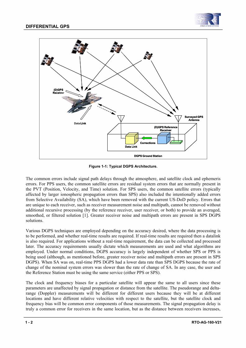
A typical DGPS architecture is shown in Figure 1-1. The system consists of a Reference Receiver (RR) located at a known location that has been previously surveyed, and one or more DGPS User Receivers (UR). The RR antenna, differential correction processing system, and datalink equipment (if used) are collectively called the Reference Station (RS). Both the UR and the RR data can be collected and stored for later processing, or sent to the desired location in real time via the datalink. DGPS is based on the principle that receivers in the same vicinity will simultaneously experience common errors on a particular satellite ranging signal. In general, the UR (mobile receivers) use measurements from the RR to remove the common errors. In order to accomplish this, the UR must simultaneously use a subset or the same set of satellites as the reference station. The DGPS positioning equations are formulated so that the common errors cancel.

DIFFERENTIAL GPS

1 - 2 RTO-AG-160-V21

CorrectionsData Link

(D)GPS Reference Receiver

Surveyed GPS Antenna

Data Link

(D)GPS Receiver

DGPS Ground Station

CorrectionsData Link

(D)GPS Reference Receiver

Surveyed GPS Antenna

Link

(D)GPS Receiver

DGPS Ground Station

Figure 1-1: Typical DGPS Architecture.

The common errors include signal path delays through the atmosphere, and satellite clock and ephemeris errors. For PPS users, the common satellite errors are residual system errors that are normally present in the PVT (Position, Velocity, and Time) solution. For SPS users, the common satellite errors (typically affected by larger ionospheric propagation errors than SPS) also included the intentionally added errors from Selective Availability (SA), which have been removed with the current US-DoD policy. Errors that are unique to each receiver, such as receiver measurement noise and multipath, cannot be removed without additional recursive processing (by the reference receiver, user receiver, or both) to provide an averaged, smoothed, or filtered solution [1]. Greater receiver noise and multipath errors are present in SPS DGPS solutions.

Various DGPS techniques are employed depending on the accuracy desired, where the data processing is to be performed, and whether real-time results are required. If real-time results are required then a datalink is also required. For applications without a real-time requirement, the data can be collected and processed later. The accuracy requirements usually dictate which measurements are used and what algorithms are employed. Under normal conditions, DGPS accuracy is largely independent of whether SPS or PPS is being used (although, as mentioned before, greater receiver noise and multipath errors are present in SPS DGPS). When SA was on, real-time PPS DGPS had a lower data rate than SPS DGPS because the rate of change of the nominal system errors was slower than the rate of change of SA. In any case, the user and the Reference Station must be using the same service (either PPS or SPS).

The clock and frequency biases for a particular satellite will appear the same to all users since these parameters are unaffected by signal propagation or distance from the satellite. The pseudorange and delta-range (Doppler) measurements will be different for different users because they will be at different locations and have different relative velocities with respect to the satellite, but the satellite clock and frequency bias will be common error components of those measurements. The signal propagation delay is truly a common error for receivers in the same location, but as the distance between receivers increases,

DIFFERENTIAL GPS

RTO-AG-160-V21 1 - 3

this error gradually de-correlates and becomes independent. The satellite ephemeris has errors in all three dimensions. Therefore, part of the error will appear as a common range error and part will remain a residual ephemeris error. The residual portion is normally small and its impact is small for similar observation angles to the satellite.

The accepted standard for SPS DGPS was developed by the Radio Technical Commission for Maritime Services (RTCM) Special Committee-104 [2, 3]. The RTCM developed standards for use of differential corrections, and defined the data format to be used between the reference station and the user. The data interchange format for NATO PPS DGPS is documented in STANAG 4392. The SPS reversionary mode specified in STANAG 4392 is compatible with the RTCM SC-104 standards. The standards are primarily intended for real-time operational use and cover a wide range of DGPS measurement types. Most SPS DGPS receivers are compatible with the RTCM SC-104 differential message formats. DGPS standards have also been developed by the Radio Technical Commission for Aeronautics (RTCA) for special Category-I (CAT-I) precision approach using range-code differential. The standards are contained in RTCA document DO-217. This document is intended only for limited use until an international standard can be developed for precision approach [4].

1.3 DGPS IMPLEMENTATION TYPES

There are two primary variations of the differential measurements and equations. One is based on ranging-code measurements and the other is based on carrier-phase measurements. There are also several ways to implement the datalink function. DGPS systems can be designed to serve a limited area from a single reference station, or can use a network of reference stations and special algorithms to extend the validity of the DGPS technique over a wide area. The result is that there is a large variety of possible DGPS system implementations using combinations of these design features.

1.3.1 Ranging-Code Differential GPS The ranging-code differential technique uses the pseudorange measurements of the RS to calculate pseudorange or position corrections for the UR. The RS calculates pseudorange corrections for each visible satellite by subtracting the “true” range determined by the surveyed position and the known orbit parameters from the measured pseudorange. The UR receiver then selects the appropriate correction for each satellite that it is tracking, and subtracts the correction from the pseudorange that it has measured. The mobile receiver must only use those satellites for which corrections have been received.

If the RS provides position corrections rather than pseudorange corrections, the corrections are simply determined by subtracting the measured position from the surveyed position. The advantage of using position corrections is obviously the simplicity of the calculations. The disadvantage is that the reference receiver and the user receiver must use the exact same set of satellites. This can be accomplished by coordinating the choice of satellite between the RR and the UR, or by having the RS compute a position correction for each possible combination of satellites. For these reasons, it is usually more flexible and efficient to provide pseudorange corrections rather than position corrections. The RTCM SC-104, NATO STANAG 4392, and RTCA DO-217 formats are all based on pseudorange rather than position corrections.

The pseudorange or position corrections are time tagged with the time that the measurements were taken. In real-time systems, the rate of change of the corrections is also calculated. This allows the user to propagate the corrections to the time that they are actually applied to the user position solution. This reduces the impact of data latency on the accuracy of the system, but does not eliminate it entirely. SPS corrections become fully uncorrelated with the user measurements after about 2 minutes. Corrections used after two minutes may produce solutions which are less accurate than stand-alone SPS GPS. PPS corrections can remain correlated with the user measurements for 10 minutes or more under benign (slowly changing) ionospheric conditions.

DIFFERENTIAL GPS

1 - 4 RTO-AG-160-V21

There are two ways of pseudorange data processing: post-mission and real-time processing. The advantage of the post-mission solution over the real-time one, is that it is more accurate, because the user can easily detect blunders and analyse the residuals of the solution. On the other hand the main disadvantage of the post-mission solution is that the results are not available immediately for navigation. The typical algorithm of the ranging-code DGPS post-processed solution is the double difference pseudorange. The mathematical models for both single difference and double difference observables are developed in the following paragraphs.

1.3.1.1 Single Difference Between Receivers

Figure 1.2 shows the possible pseudorange measurements between two receivers (k. l) and two satellites (p, q). If pseudorange 1 and 2 from Figure 1.2 are differenced, then the satellite clock error and satellite orbit errors will be removed. Moreover, SA will be reduced and will be removed completely only if the signals transmitted to each receiver, are emitted exactly at the same time. The residual error from SA is not a problem for post-processed positioning, where it is easy to ensure that the differencing is done between pseudoranges observed at the same time [5]. Any atmospheric errors will also be reduced significantly with single differencing.

Figure 1-2: Pseudorange Differencing.

The basic mathematical model for single difference pseudorange observation is the following (refer to equation A.7 of Section A.4 in Annex A):

( )P P dt dt c d d d dkp

lp

kp

lp

k l k p l p k pp

l pp

p− = − − − + − + − +ρ ρ ε, , , , ∆ (1.1)

DIFFERENTIAL GPS

RTO-AG-160-V21 1 - 5

where Pip is the pseudorange measurement, ρi

p denotes the geometric distance between the stations and satellite, dti denotes the receiver’s clock offsets, di p, denotes the receiver’s hardware code delays, di p

p,

denotes the multipath of the codes, ∆ε p denotes the measurement noise and c is the velocity of light. Equation (1.1) represents the single difference pseudorange observable between receivers. Another type of single difference apart from (1.1), is known as between-satellite single difference.

There are four unknowns in equation (1.1) assuming that the co-ordinates of station k are known and that the difference in clock drifts is one unknown. Hence, four satellites are required to provide four single difference equations in order to solve for the unknowns. Single differences with code observations are frequently used in relative (differential) navigation [6].

1.3.1.2 Double Difference Observable

Using all pseudoranges shown in Figure 1-2, differences are formed between receivers and satellites. Double differences are constructed by taking two between-receiver single differences and differencing these between two satellites. This procedure removes all satellite dependent, receiver dependent and most of the atmospheric errors (if the distance between the two receivers is not too large). The derived equation is:

P P P P dkp

kq

lp

lq

kp

kq

lp

lq

i pj− − − = − − − +ρ ρ ρ ρ , (1.2)

where di pj, denotes the total effect of multipath.

There are three unknowns in equation (1.2); the co-ordinates of station l. A minimum of four satellites is required to form a minimum of three double difference equations in order to solve for the unknowns.

Using the propagation of errors law, it is shown that the double difference observables are twice as noisy as the pure pseudoranges [5]:

σ σ σ σ σ σDD P P P P P= + + + =2 2 2 2 2 (1.3)

but they are more accurate, because most of the errors are removed. Note that multipath remains, because it cannot be modelled and it is independent for each receiver.

1.3.2 Carrier-Phase Differential GPS The carrier-phase measurement technique uses the difference between the carrier phases measured at the RR and UR. A double-differencing technique is used to remove the satellite and receiver clock errors. The first difference is the difference between the phase measurement at the UR and the RR for a single satellite. This eliminates the satellite clock error which is common to both measurements. This process is then repeated for a second satellite. A second difference is then formed by subtracting the first difference for the first satellite from the first difference for the second satellite. This eliminates both receiver clock errors which are common to the first difference equations. This process is repeated for two pairs of satellites resulting in three double-differenced measurements that can be solved for the difference between the reference station and user receiver locations. This is inherently a relative positioning technique, therefore the user receiver must know the reference station location to determine its absolute position. More details of these processes are illustrated in the following subsections were the various observation equations are presented.

DIFFERENTIAL GPS

1 - 6 RTO-AG-160-V21

1.3.2.1 Single Difference Observable

The single difference is the instantaneous phase difference between two receivers and one satellite. It is also possible to define single differences between two satellites and one receiver. Using the basic definition of carrier-phase observable presented in equation (A.23) of Annex A, the phase difference between the two receivers A and B, and satellite i is given by:

( ) ( ) ( )Φ Φ ΦABi

Bi

Aiτ τ τ= − (1.4)

and can be expressed as:

( ) ( ) ( )Φ ΦABi

ABi

ABi

ABif

ct Nτ ρ τ=

⋅ + − (1.5)

where N N NABi

Bi

Ai= − . Hence, with four satellites i, j, k and l:

( ) ( ) ( )Φ ΦABi

ABi

ABi

ABif

ct Nτ ρ τ=

⋅ + − ; ( ) ( ) ( )Φ ΦAB

kABk

ABk

ABkf

ct Nτ ρ τ=

⋅ + − ;

( ) ( ) ( )Φ ΦABj

ABj

ABj

ABjf

ct Nτ ρ τ=

⋅ + − ; ( ) ( ) ( )Φ ΦAB

lABl

ABl

ABlf

ct Nτ ρ τ=

⋅ + − .

1.3.2.2 Double Difference

The double difference is formed from subtracting two single differences measured to two satellites i and j. The basic double difference equation is:

( ) ( ) ( )Φ Φ ΦABij

ABi

ABiτ τ τ= − (1.6)

which simplifies to:

( ) ( )ΦABij

ABij

ABijf

ct Nτ ρ=

− (1.7)

where N N NABij

ABj

ABi= − , and the only unknowns being the double-difference phase ambiguity NAB

ij and the receiver co-ordinates. The local clock error is differenced out.

Two receivers A and B, and four satellites i, j, k, and l, will give 3 double difference equations with unknown co-ordinates (X, Y, Z), of A and B, and the unknown integer ambiguities N AB

ij , N ABik ,

and N ABil :

( ) ( )ΦABij

ABij

ABijf

ct Nτ ρ=

− ; ( ) ( )ΦAB

ikABik

ABikf

ct Nτ ρ=

− ;

( ) ( )ΦABil

ABil

ABilf

ct Nτ ρ=

− .

Therefore, the double difference observation equation can be written as [7]:

DIFFERENTIAL GPS

RTO-AG-160-V21 1 - 7

( )

∂∂

∂∂

∂∂

∂∂

∂∂

∂∂

∂∂

∂∂

∂∂

∂∂

Φ Φ Φ Φ Φ Φ

Φ Φ Φ ΦΦ Φ

XdX

YdY

ZdZ

XdX

YdY

ZdZ

NdN

NdN

NdN

CdC v

AA

AA

AA

BB

BB

BB

O C

+ + + + +

+ + + + + = − +1

12

23

3... ... (1.8)

where: X Y ZA A A, , = Co-ordinates of Receiver A; X Y ZB B B, , = Co-ordinates of Receiver B; N N N1 2 3, , = Integer Ambiguities; C = Tropospheric Factor;

( )Φ ΦO C− = Observed minus Computed Observable; and

ν = Residual.

From equation (1.8) the unknown receiver co-ordinates can be computed. It is necessary, however, to determine the carrier phase integer ambiguities (i.e., the integer number of complete wavelengths between the receiver and satellites).

In certain surveying applications, this integer ambiguity can be resolved by starting with the mobile receiver antenna within a wavelength of the reference receiver antenna. Both receivers start with the same integer ambiguity, so the difference is zero and drops out of the double-difference equations. Thereafter, the phase shift that the mobile receiver observes (whole cycles) is the integer phase difference between the two receivers. For other applications where it is not practical to bring the reference and mobile antennas together, the reference and mobile receivers can solve for the ambiguities independently as part of an initialisation process. One way is to place the mobile receiver at a surveyed location. In this case the initial difference is not necessarily zero, but it is an easily calculated value.

For some applications, it is essential to be able to solve for integer ambiguity at an unknown location or while in motion (or both). In this case, solving for the integer ambiguity usually consists of eliminating incorrect solutions until the correct solution is found. A good initial estimate of position (such as from ranging-code differential) helps to keep the initial number of candidate solutions small [8]. Redundant measurements over time and/or from extra satellite signals are used to isolate the correct solution. These “search” techniques can take as little as a few seconds or up to several minutes to perform and can require significant computer processing power. This version of the carrier-phase DGPS technique is typically called “Kinematic GPS” (KGPS). If carrier track or phase lock on a satellite is interrupted (cycle slip) and the integer count is lost, then the initialisation process must be repeated for that satellite. Causes of cycle slips range from physical obstruction of the antenna to the sudden acceleration of the user platform. Output data flow may also be interrupted if the receiver is not collecting redundant measurements form extra satellites to maintain the position solution. If a precise position solution is maintained, re-initialisation for the “lost” satellite can be almost immediate.

Developing a robust and rapid method of initialisation and re-initialisation is the primary challenge facing designers of real-time systems that have a safety critical application such as aircraft precision approach. A description of techniques for solving ambiguities both in real-time and post-processing applications, together with information about cycle slips repair techniques can be found in the references [9 – 17].

1.3.3 DGPS Datalink Implementations DGPS can also be implemented in several different ways depending on the type of datalink used. The simplest way is no datalink at all. For non-real-time applications, the measurements can be stored in

DIFFERENTIAL GPS

1 - 8 RTO-AG-160-V21

the receiver or on suitable media and processed at a later time. In most cases to achieve surveying accuracies, the data must be post-processed using precise ephemeris data that is only available after the survey data has been collected. Similarly, for some test applications the cost and effort to maintain a real-time datalink may be unnecessary. Nevertheless, low-precision real-time outputs can be useful to confirm that a test is progressing properly even if the accuracy of the results will be enhanced later. Differential corrections or measurements can be uplinked in real-time from the reference station to the users. This is the most common technique where a large number of users must be served in real-time. For military purposes and proprietary commercial services, the uplink can be encrypted to restrict the use of the DGPS signals to a selected group of users. Differential corrections can be transmitted to the user at different frequencies. With the exception of satellite datalinks there is generally a trade-off between the range of the system and the update rate of the corrections [18, 19]. As an example Table 1-1 lists a number of frequency bands, the range, and the rate at which the corrections could be updated using the standard RTCM SC-104 format [2, 3, 20].

Table 1-1: DGPS Datalink Frequencies

Frequency Range (km) Update Rate (sec)

LF (30 – 300 kHz) > 700 < 20

MF (300 kHz – 3 MHz) < 500 5 – 10

HF ( 3 MHz – 25 MHz) < 200 5

VHF (30 MHz – 300 MHz) < 100 < 5

L Band (1 GHz – 2 GHz) Line of Sight Few Seconds

An uplink can be a separate transmitter/receiver system or the DGPS signals can be superimposed on a GPS-link L-band ranging signal. The uplink acts as a pseudo-satellite or “pseudolite” and delivers the ranging signal and DGPS data via the RF section of the user receiver, much in the same way the GPS navigation message is transmitted. The advantages are that the additional ranging signal(s) can increase the availability of the position solution and decrease carrier-phase initialisation time. However, the RS and URs become more complex, and the system has a very short range (a few kilometres at the most). This is not only because of the line of sight restriction, but also the power must be kept low in order to avoid interference with the real satellite signals (i.e., the pseudolite can become a GPS jammer if it overpowers the GPS satellite signals).

A downlink option is also possible from the users to the RS or other central collection point. In this case the differential solutions are all calculated at a central location. This is often the case for test range applications where precise vehicle tracking is desired, but the information is not used aboard the vehicle. The downlink data can be position data plus the satellite tracked, or pseudorange and deltarange measurements, or it can be the raw GPS signals translated to an intermediate frequency. The translator method can often be the least expensive with respect to user equipment, and therefore is often used in munitions testing where the user equipment may be expendable. More details about these applications are given in Chapter 4.

1.3.4 Local Area and Wide Area DGPS The accuracy of a DGPS solution developed using a single RS will degrade with distance from the RS site. This is due to the increasing difference between the reference and the user receiver ephemeris,

DIFFERENTIAL GPS

RTO-AG-160-V21 1 - 9

ionospheric, and tropospheric errors. The errors are likely to remain highly correlated within a distance of 350 km [20], but practical systems are often limited by the datalink to an effective range of around 170 km. Such systems are usually called Local Area DGPS (LADGPS).

DGPS systems that compensate for accuracy degradation over large areas are referred to as wide area DGPS (WADGPS) systems. They usually employ a network of reference receivers that are coordinated to provide DGPS data that is valid over a wide coverage area. Such systems typically are designed to broadcast the DGPS data via satellite, although a network of ground transmission sites is also feasible. A user receiver typically must employ special algorithms to derive the ionospheric and tropospheric corrections that are appropriate for its location from the observations taken at the various reference sites.

The United States, Canada, Europe, Japan, and Australia have developed or are planning to deploy WADGPS systems transmitting from geostationary satellites for use by commercial aviation [21]. The satellites can also provide GPS-like ranging signals. Other nations may participate by providing clock corrections only from single sites or small networks, requiring the user to derive ionospheric corrections from an ionospheric model or dual-frequency measurements. Some commercial DGPS services broadcast the data from multiple reference stations via satellite. However, several such systems remain a group of LADGPS rather than WADGPS systems. This is because the reference stations are not integrated into a network, therefore the user accuracy degrades with distance from the individual reference sites.

1.4 DGPS ACCURACY Controlled tests and recent extensive operational use of DGPS, have repeatedly demonstrated that DGPS (pseudorange) results in an accuracy of the order of about 10 metres. This figure is largely irrespective of receiver type, whether or not SA is in use, and over distances of up to 500 km from the Reference Station [23, 24]. With KGPS positioning systems, requiring the resolution of the carrier phase integer ambiguities whilst on the move, centimetre level accuracy can be achieved [9, 25].

Many recent applications of DGPS use C/A code pseudorange as the only observable, with achieved accuracies of 1 to 5 m in real-time. Other applications use both pseudorange (C/A or P code) and carrier phase observables. Very Precise DGPS (VPDGPS) and Ultra Precise DGPS (UPDGPS) are the state-of-the-art ASHTECH packages, taking advantage of precise dual band P code pseudorange and carrier phase observables and is capable of On-The-Fly (OTF) ambiguity resolution. ASHTECH has developed various techniques which achieve increased accuracy at the expense of increased complexity (many other receiver manufacturers deliver likewise solutions). The ASHTECH classification scheme of these techniques is presented in Table 1-2 [26].

Table 1-2: ASHTECH Classification Scheme of DGPS Techniques

Name Description RMS

DGPS C/A code pseudorange 1 – 5 m

PDGPS P code pseudorange 0.1 – 1 m

VPDGPS Addition of dual band carrier phase 5 – 30 cm

UPDGPS Above with integer ambiguities resolved < 2 cm

A discussion of DGPS error sources is presented below, together with a comparison between non-differential GPS and DGPS error budgets.

DIFFERENTIAL GPS

1 - 10 RTO-AG-160-V21

1.5 DGPS ERROR SOURCES

The major sources of error affecting stand-alone GPS (see Annex A) are the following:

• Ephemeris Error;

• Ionospheric Propagation Delay;

• Tropospheric Propagation Delay;

• Satellite Clock Drift;

• Multipath;

• Receiver Noise and clock drift; and

• Selective Availability Errors (only SPS applications).

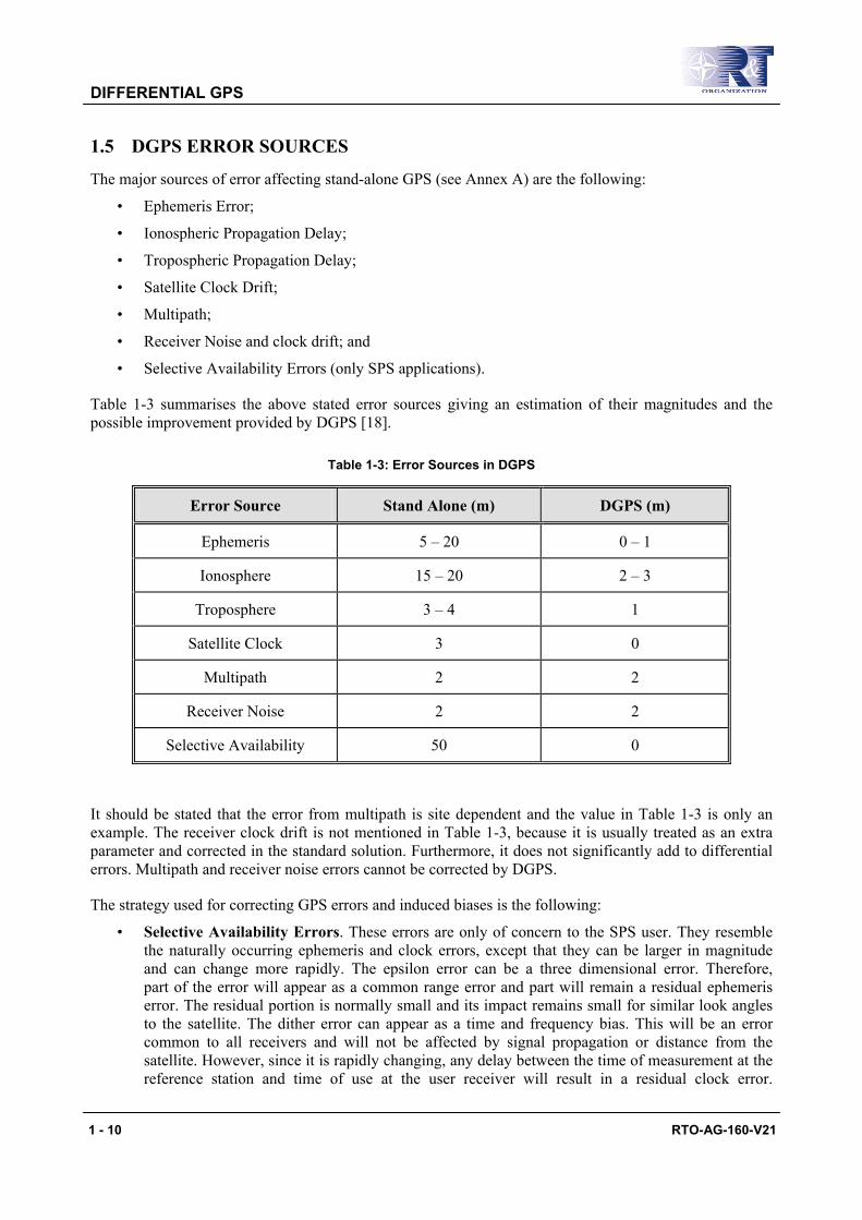
Table 1-3 summarises the above stated error sources giving an estimation of their magnitudes and the possible improvement provided by DGPS [18].

Table 1-3: Error Sources in DGPS

Error Source Stand Alone (m) DGPS (m)

Ephemeris 5 – 20 0 – 1

Ionosphere 15 – 20 2 – 3

Troposphere 3 – 4 1

Satellite Clock 3 0

Multipath 2 2

Receiver Noise 2 2

Selective Availability 50 0

It should be stated that the error from multipath is site dependent and the value in Table 1-3 is only an example. The receiver clock drift is not mentioned in Table 1-3, because it is usually treated as an extra parameter and corrected in the standard solution. Furthermore, it does not significantly add to differential errors. Multipath and receiver noise errors cannot be corrected by DGPS.

The strategy used for correcting GPS errors and induced biases is the following:

• Selective Availability Errors. These errors are only of concern to the SPS user. They resemble the naturally occurring ephemeris and clock errors, except that they can be larger in magnitude and can change more rapidly. The epsilon error can be a three dimensional error. Therefore, part of the error will appear as a common range error and part will remain a residual ephemeris error. The residual portion is normally small and its impact remains small for similar look angles to the satellite. The dither error can appear as a time and frequency bias. This will be an error common to all receivers and will not be affected by signal propagation or distance from the satellite. However, since it is rapidly changing, any delay between the time of measurement at the reference station and time of use at the user receiver will result in a residual clock error.

DIFFERENTIAL GPS

RTO-AG-160-V21 1 - 11

SPS DGPS systems are normally designed with a rate-of-change term in the corrections and rapid update rates to minimise this effect.

• Ionospheric and Tropospheric Delays. For users near the reference station, the respective signal paths to the satellite are close enough together that the compensation is almost complete. As the user to RS separation is increased, the different ionospheric and tropospheric paths to the satellites can be far enough apart that the ionospheric and tropospheric delays are no longer common errors. Thus, as the distance between the RS and user receiver increases the effectiveness of the atmospheric delay corrections decreases.

• Ephemeris Error. This error is effectively compensated unless it has quite a large out-of-range component (e.g., 1000 metres or more due to an error in a satellite navigation message). Even then, the error will be small if the distance between the reference receiver and user receiver is small.

• Satellite Clock Error. Except in a satellite failure situation, this error is more slowly changing than the SA dither error. For all practical purposes, this error is completely compensated, as long as both reference and user receivers employ the same satellite clock correction data.

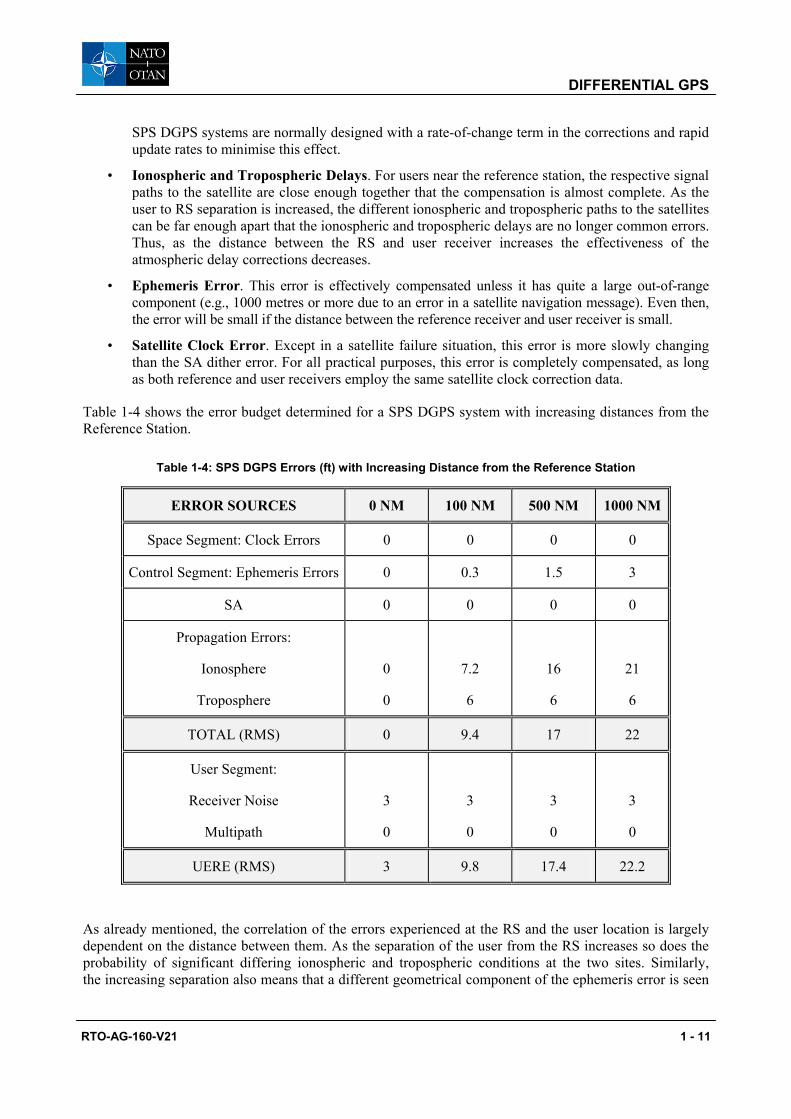
Table 1-4 shows the error budget determined for a SPS DGPS system with increasing distances from the Reference Station.

Table 1-4: SPS DGPS Errors (ft) with Increasing Distance from the Reference Station

ERROR SOURCES 0 NM 100 NM 500 NM 1000 NM

Space Segment: Clock Errors 0 0 0 0

Control Segment: Ephemeris Errors 0 0.3 1.5 3

SA 0 0 0 0

Propagation Errors:

Ionosphere

Troposphere

0

0

7.2

6

16

6

21

6

TOTAL (RMS) 0 9.4 17 22

User Segment:

Receiver Noise

Multipath

3

0

3

0

3

0

3

0

UERE (RMS) 3 9.8 17.4 22.2

As already mentioned, the correlation of the errors experienced at the RS and the user location is largely dependent on the distance between them. As the separation of the user from the RS increases so does the probability of significant differing ionospheric and tropospheric conditions at the two sites. Similarly, the increasing separation also means that a different geometrical component of the ephemeris error is seen

DIFFERENTIAL GPS

1 - 12 RTO-AG-160-V21

by the RR and UR. This is commonly referred to as “Spatial Decorrelation” of the ephemeris and atmospheric errors. In general, the errors are highly correlated for a user within 350 km of the RS. In most cases however, if the distance is greater than 250 km the user will obtain better results using correction models for ionospheric and tropospheric delay [18, 27]. Since the RR noise and multipath errors are included in the differential corrections and become part of the user’s error budget (root-sum-squared with the user receiver noise and multipath errors), the receiver noise and multipath error components in the non-differential receiver can be lower than the correspondent error components experienced in the DGPS implementation.

The other type of error introduced in real-time DGPS positioning systems is the datalink “age of corrections”. This error is introduced due to the latency of the transmitted corrections (i.e., the transmitted corrections of epoch t0 arrive at the moving receiver at epoch t dt0 + ). These corrections are not the correct ones, because they were calculated under different SA/AS conditions. Hence, the co-ordinates of the UR would be slightly offset.

1.6 INTEGRITY ISSUES FOR AIRCRAFT NAVIGATION At the moment, satellite navigation systems are only certified to be used as a supplementary mean of aircraft navigation. Contrary to the systems in use, GPS is, as yet, only certifiable for aircraft navigation if it is integrated with other navigation systems. The reason is not the accuracy but integrity. According to the US Federal Radionavigation Plan [28], “Integrity is the ability of a system to provide timely warnings to users when the system should not be used for navigation”. Another definition is: “With probability P, either the horizontal radial position error does not exceed a pre-specified threshold R, or an alarm is raised within a time-to alarm interval of duration T when the horizontal radial position error exceeds a pre-specified threshold R”. To detect that the error is exceeding a threshold, a monitor function has to be installed within the navigation system. This is also the case within the GPS system in the form of the ground segment. However, for this system, the time to alarm (TTA) is in the order of several hours, that is even too long for the cruise where a TTA of 60 seconds is required (an autoland system for zero meter vertical visibility must not exceed a TTA of 2 seconds). Various methods have been proposed and practically implemented for stand-alone GPS integrity monitoring. A growing family of such implementations, already very popular in aviation applications, includes the so called Receiver Autonomous Integrity Monitoring (RAIM) techniques. Details about RAIM techniques can be found in the references [4, 22].

Regarding DGPS, it should be underlined that it does more than increasing the GPS positioning accuracy, it also enhances GPS integrity by compensating for anomalies in the satellite ranging signals and navigation data message. The range and range rate corrections provided in the ranging-code DGPS correction message can compensate for ramp and step type anomalies in the individual satellite signals, until the corrections exceed the maximum values or rates allowed in the correction format. If these limits are exceeded, the user can be warned not to use a particular satellite by placing “do-not-use” bit patterns in the corrections for that satellite (as defined in STANAG 4392 or RTCM SC-104 message formats) or by omitting the corrections for that satellite. As mentioned before, step anomalies will normally cause carrier-phase DGPS receivers to lose lock on the carrier phase, causing the reference and user receivers to reinitialise. UR noise, processing anomalies, and multipath at the user GPS antenna cannot be corrected by a DGPS system. These errors are included in the overall DGPS error budget.

Errors in determining or transmitting the satellite corrections may be passed on to the differential user if integrity checks are not provided within the RS. These errors can include inaccuracies in the RS antenna location that bias the corrections, systematic multipath due to poor antenna sighting (usually in low elevation angle satellites), algorithmic errors, receiver inter-channel bias errors, receiver clock errors, and communication errors. For these reasons, typical WADGPS and LADGPS RS designs also include integrity checking provisions to guarantee the validity of the corrections before and after broadcast [21, 29].

DIFFERENTIAL GPS

RTO-AG-160-V21 1 - 13

1.7 DGPS AUGMENTATION SYSTEMS

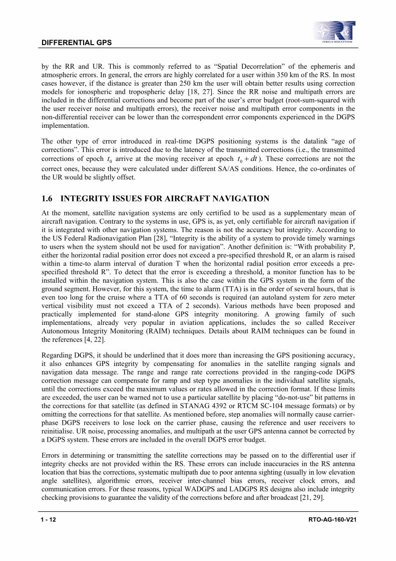
Various strategies have been developed for increasing the levels of integrity, accuracy and availability of DGPS-based navigation/landing systems. These include both Space-Based Augmentation Systems (SBAS) and Ground-Based Augmentation Systems (GBAS). Particularly, the American Wide Area Augmentation System (WAAS) and the European Geostationary Navigation Overlay System (EGNOS) are examples of SBAS. In these systems, geostationary satellites (INMARSAT-3) are used to broadcast various signals, computed through a ground network of Integrity Monitoring Stations and transmitted from a dedicated Earth Station. In the case of WAAS (Figure 1-3), the geostationary (GEO) satellites broadcast the following [30]:

• GPS Use/Don’t Use Warning (Integrity Signals);

• Corrections for each SV: clock, ephemeris, ionospheric (to increase Accuracy); and

• Ranging Signals (to increase Availability).

Integrity MonitoringStations

Space Segment

GPS

User Segment

Navigation Earth Station( Primary / Standby )

IntegrityProcessing

Ground Segment

INMARSAT-3

Indicated Location

True Location

•Vector Corrections•Use/Don’t Use•Ranging Signal

Atmospheric Effects

Figure 1-3: Wide Area Augmentation System.

WAAS is designed to provide precision approach capability (3-dimensional guidance) for Category 1 (CAT-1) approaches with the following availability:

• Better Than 95% Available in the majority of Continental US (CONUS); and

• Rest of U.S. – Available, but less than 95%.

Furthermore, for en-route through non-precision approaches the following availability is specified:

• 50% of Continental US – Better than 99.9% Availability; and

• Rest of U.S. – Available, but less than 99.9%.

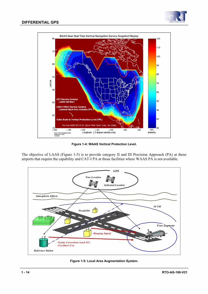
The Vertical Protection Level (VPL) currently offered by the WAAS service in CONUS is shown in Figure 1-4.

DIFFERENTIAL GPS

1 - 14 RTO-AG-160-V21

Figure 1-4: WAAS Vertical Protection Level.

The objective of LAAS (Figure 1-5) is to provide category II and III Precision Approach (PA) at those airports that require the capability and CAT-I PA at those facilities where WAAS PA is not available.

Pseudolite

GPS

User Segment

Reference Station

Indicated Location

True Location

•Scalar Corrections (each SV)•Use/Don’t Use

Atmospheric Effects

•Ranging Signal

50 NM

Figure 1-5: Local Area Augmentation System.

DIFFERENTIAL GPS

RTO-AG-160-V21 1 - 15

For this purpose, the Local Reference Station broadcasts:

• GPS Use/Don’t Use Warning (to increase Integrity); and

• Scalar Corrections (to increase Accuracy).

Local Pseudolites Broadcasting (LPB) is implemented in order to make available additional ranging signals for an increased availability and accuracy [31]. More detailed information about recent LAAS, WAAS and Pseudolites systems developments can be found in the references [30 – 33].

1.8 REFERENCES

[1] Chao, C.H. (1998). “High Precision Differential GPS”. MSc Dissertation. Institute of Engineering Surveying and Space Geodesy (Institute of Engineering Surveying and Space Geodesy (IESSG)) – University of Nottingham.

[2] RTCM Special Committee No. 104. (1990). “RTCM Recommended Standards for Differential NAVSTAR GPS Service”. Radio Technical Committee for Maritime Services. Paper 134-89/SC104-68. Washington DC (USA).

[3] RTCM Special Committee No. 104. (1994). “RTCM Recommended Standards for Differential NAVSTAR GPS Service”. Radio Technical Committee for Maritime Services. Paper 194-93/SC104-STD. Washington DC (USA).

[4] Joint Program Office (JPO). (1997). “NAVSTAR GPS User Equipment, Introduction”. Public Release Version. US Air Force Space Systems Division, NAVSTAR-GPS Joint Program Office (JPO). Los Angeles AFB, California (USA).

[5] Walsh, D. (1994). “Kinematic GPS Ambiguity Resolution”. PhD Thesis, Institute of Engineering Surveying and Space Geodesy (IESSG), University of Nottingham.

[6] Seeber, G. (1994). “Satellite Geodesy”. Second Edition. Artech House Publishers. New York (USA).

[7] Ashkenazi, V. (1997). “Principles of GPS and Observables”. Lecture Notes, Institute of Engineering Surveying and Space Geodesy (IESSG) – University of Nottingham.

[8] Ashkenazi, V., Moore, T. and Westrop, J.M. (1990). “Combining Pseudo-range and Phase for Dynamic GPS”. Paper presented at the International Symposium on Kinematic Systems in Geodesy, Surveying and Remote Sensing. London (UK).

[9] Ashkenazi, V., Foulkes-Jones, G.H., Moore, T. and Walsh, D. (1993). “Real-time Navigation to Centimetre Level”. Paper presented at DSNS93, the 2nd International Symposium on Differential Navigation. Amsterdam (The Netherlands).

[10] Euler, H.J. and Landau, H. (1992). “Fast GPS Ambiguity Resolution On-The-Fly for Real-time Applications”. Paper presented at the 6th International Geodetic Symposium on Satellite Positioning. Columbus (Ohio).

[11] Euler, H.J. (1994). “Achieving high-accuracy relative positioning in real-time: system design, performance and real-time results”. Proceedings of the 4th IEEE Plans Conference. Las Vegas (NV).

[12] Hansen, P. (1994). “Real-time GPS Carrier Phase Navigation”. The University of Nottingham, Institute of Engineering Surveying and Space Geodesy (IESSG). Paper presented at the DSNS-94 Conference. London (UK).

DIFFERENTIAL GPS

1 - 16 RTO-AG-160-V21

[13] Hatch, R.R. (1990). “Instantaneous Ambiguity Resolution”. Presented at the KIS Symposium. Banff (Canada).

[14] Hatch, R.R. (1991). “Ambiguity Resolution While Moving, Experimental Results”. Proc. of ION GPS-91, the 4th International Technical Meeting of the Satellite Division of the US Institute of Navigation. Albuquerque (NM).

[15] Kleusberg, A. (1986). “Kinematic Relative Positioning Using GPS Code and Carrier Beat Phase Observations”. 2nd Marine Geodesy Symposium. London (UK).

[16] Landau, H. (1992). “On-The-Fly Ambiguity Resolution Using Differential P-code Group and Phase Delay Measurements”. 5th International Technical Meeting of the Satellite Division of the US Institute of Navigation. Orlando (USA).

[17] Mader, G. (1986). “Dynamic Positioning using GPS Carrier Phase Measurements”. Manuscripte Geodaetica. Volume 36 (86).

[18] Moore, T. (2002). “An Introduction to Differential GPS”. Lecture Notes, Institute of Engineering Surveying and Space Geodesy (IESSG) – University of Nottingham (UK).

[19] Moore, T. (2002). “GPS Orbit Determination and Fiducial Networks”. Lecture Notes, Institute of Engineering Surveying and Space Geodesy (IESSG) – University of Nottingham (UK).

[20] Cross, P.A. and Roberts, W.D.S. (1990). “Differential Offshore Positioning using Block II GPS Satellites”. 7th International Symposium of the Hydrographic Society (Hydro ‘90). Southampton (UK).

[21] Keith, A. (2000). “Using Wide Area Differential GPS to improve total system error for precision flight Operations”. PhD Thesis. Stanford University (USA).

[22] Parkinson, B.W., Spilker, J.J., Jr. Editors. (1996). “Global Positioning System: Theory and Applications – Volume II”. Progress in Astronautics and Aeronautics. Vol. 163. Published by the American Institute of Aeronautics and Astronautics.

[23] Moore, T. (2002). “Other Satellite Navigation Systems”. Lecture Notes, Institute of Engineering Surveying and Space Geodesy (IESSG) – University of Nottingham (UK).

[24] Yuan, J., Gu, X., Jacob, T. and Schanzer, G. (1990). “Error Correction for Differential GPD with Long Separated Ground Stations and User for Aircraft Landing”. Institute of Guidance and Control. Technical University Braunschweig (Germany).

[25] Ashkenazi, V., Summerfield, P. and Westrop, J. (1990). “Kinematic Positioning by GPS”. Tiré a part des Cahiers du Centre Européen de Géodynamique et de Séismologie, Volume 2.

[26] Qin, X., Gourevitch, S. and Kuhl, M. (1992). “Very Precise Differential GPS – Development Status and Test Results”. Proc. of ION GPS-92, 5th International Technical Meeting of the Satellite Division of the US Institute of Navigation. Albuquerque (USA).

[27] Dodson, A.H. (2002). “Propagation Effects on GPS Measurements”. Lecture Notes, Institute of Engineering Surveying and Space Geodesy (IESSG) – University of Nottingham (UK).

[28] US Department of Defence and US Department of Transportation. (2001). “Federal Radionavigation Plan – 2001”. National Technical Information Services. Springfield (USA). Doc. DOT-VNTSC-RSPA-01-3/DOD-4650.5.

DIFFERENTIAL GPS

RTO-AG-160-V21 1 - 17

[29] Ko, P.Y. (1997). “Wide Area Differential GPS (WADGPS)”. PhD Thesis. Stanford University (USA).

[30] Dye, S. and Baylin, F. (2004). “The GPS Manual Principles and Applications”. Second Edition. Baylin Publications (USA).

[31] Cobb, S.A. (1997). “GPS Pseudolites: Theory, Design and Applications”. PhD Dissertation. Stanford University (USA).

[32] Chao, Y. (1997). “Real Time Implementation of Wide Area Augmentation System for Global Positioning with an Emphasis on Ionospheric Modeling”. PhD Thesis. Stanford University (USA).

[33] Lee, J.S. (2005). “GPS-Based Aircraft Landing Systems with Enhanced Performance Beyond Accuracy”. PhD Dissertation. Stanford University (USA).

DIFFERENTIAL GPS

1 - 18 RTO-AG-160-V21

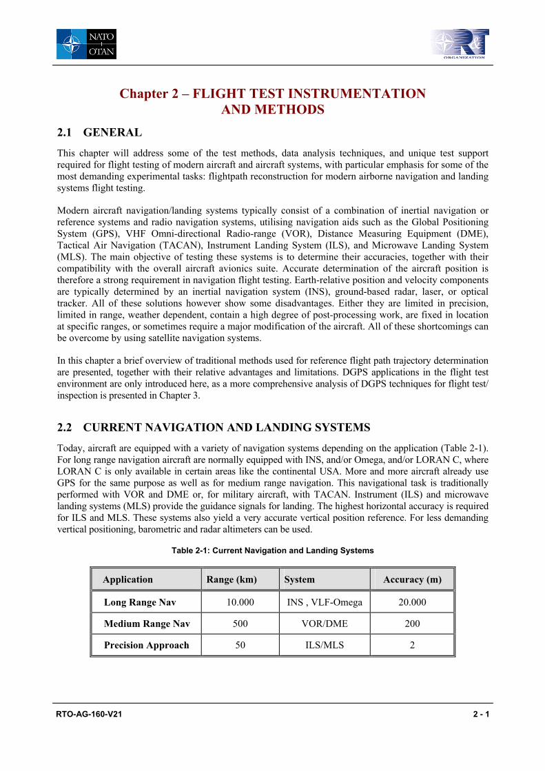
RTO-AG-160-V21 2 - 1

Chapter 2 – FLIGHT TEST INSTRUMENTATION AND METHODS

2.1 GENERAL

This chapter will address some of the test methods, data analysis techniques, and unique test support required for flight testing of modern aircraft and aircraft systems, with particular emphasis for some of the most demanding experimental tasks: flightpath reconstruction for modern airborne navigation and landing systems flight testing.

Modern aircraft navigation/landing systems typically consist of a combination of inertial navigation or reference systems and radio navigation systems, utilising navigation aids such as the Global Positioning System (GPS), VHF Omni-directional Radio-range (VOR), Distance Measuring Equipment (DME), Tactical Air Navigation (TACAN), Instrument Landing System (ILS), and Microwave Landing System (MLS). The main objective of testing these systems is to determine their accuracies, together with their compatibility with the overall aircraft avionics suite. Accurate determination of the aircraft position is therefore a strong requirement in navigation flight testing. Earth-relative position and velocity components are typically determined by an inertial navigation system (INS), ground-based radar, laser, or optical tracker. All of these solutions however show some disadvantages. Either they are limited in precision, limited in range, weather dependent, contain a high degree of post-processing work, are fixed in location at specific ranges, or sometimes require a major modification of the aircraft. All of these shortcomings can be overcome by using satellite navigation systems.

In this chapter a brief overview of traditional methods used for reference flight path trajectory determination are presented, together with their relative advantages and limitations. DGPS applications in the flight test environment are only introduced here, as a more comprehensive analysis of DGPS techniques for flight test/ inspection is presented in Chapter 3.

2.2 CURRENT NAVIGATION AND LANDING SYSTEMS

Today, aircraft are equipped with a variety of navigation systems depending on the application (Table 2-1). For long range navigation aircraft are normally equipped with INS, and/or Omega, and/or LORAN C, where LORAN C is only available in certain areas like the continental USA. More and more aircraft already use GPS for the same purpose as well as for medium range navigation. This navigational task is traditionally performed with VOR and DME or, for military aircraft, with TACAN. Instrument (ILS) and microwave landing systems (MLS) provide the guidance signals for landing. The highest horizontal accuracy is required for ILS and MLS. These systems also yield a very accurate vertical position reference. For less demanding vertical positioning, barometric and radar altimeters can be used.

Table 2-1: Current Navigation and Landing Systems

Application Range (km) System Accuracy (m)

Long Range Nav 10.000 INS , VLF-Omega 20.000

Medium Range Nav 500 VOR/DME 200

Precision Approach 50 ILS/MLS 2

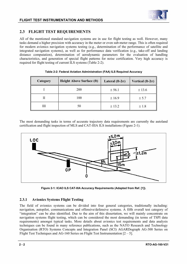
FLIGHT TEST INSTRUMENTATION AND METHODS

2 - 2 RTO-AG-160-V21

2.3 FLIGHT TEST REQUIREMENTS

All of the mentioned standard navigation systems are in use for flight testing as well. However, many tasks demand a higher precision with accuracy in the meter or even sub-meter range. This is often required for modern avionics navigation systems testing (e.g., determination of the performance of satellite and integrated navigation systems), as well as for performance data verification (e.g., take-off and landing distance computation), determination of aerodynamic parameters for the evaluation of handling characteristics, and generation of special flight patterns for noise certification. Very high accuracy is required for flight testing of current ILS systems (Table 2-2).

Table 2-2: Federal Aviation Administration (FAA) ILS Required Accuracy

Category Height Above Surface (ft) Lateral (ft-2σ) Vertical (ft-2σ)

I 200 ± 56.1 ± 13.6

II 100 ± 16.9 ± 5.7

III 50 ± 13.2 ± 1.8

The most demanding tasks in terms of accurate trajectory data requirements are currently the autoland certification and flight inspection of MLS and CAT-IIIA ILS installations (Figure 2-1).

Figure 2-1: ICAO ILS CAT-IIIA Accuracy Requirements (Adapted from Ref. [1]).

2.3.1 Avionics Systems Flight Testing The field of avionics systems can be divided into four general categories, traditionally including: navigation, autopilot, communications and offensive/defensive systems. A fifth overall test category of “integration” can be also identified. Due to the aim of this dissertation, we will mainly concentrate on navigation systems flight testing, which can be considered the most demanding (in terms of TSPI data requirements) amongst typical tasks. More details about avionics test requirements and data analysis techniques can be found in many reference publications, such as the NATO Research and Technology Organisation (RTO) Systems Concepts and Integration Panel (SCI) AGARDograph AG-300 Series on Flight Test Techniques and AG-160 Series on Flight Test Instrumentation [2 – 5].

FLIGHT TEST INSTRUMENTATION AND METHODS

RTO-AG-160-V21 2 - 3

2.3.1.1 Navigation Systems

The primary objectives of flight testing aircraft navigation systems is to evaluate the following:

• System accuracy (latitude/longitude, range, bearing, glide slope, etc.);

• System error rates (latitude error rate, longitude error rate, radial error rate);

• System functionality (modes and displays perform as designed);

• System operational suitability (system ability to provide acceptable navigation capabilities for the intended operational applications); and

• System electromagnetic compatibility and resistance to jamming.

The assessment of navigation system performance is generally divided into two parts, navigation accuracy and guidance accuracy, both laterally and vertically. Full-up performance in this case is similar to fault free performance, it means all system inputs are available. Loss of an input need not be due to a failure, but could result from loss or degradation of a radio navigation sensor due to propagation conditions.

The objective of navigation accuracy testing is to measure how well the navigation system determines the actual aircraft position. This need not always be a complicated test. It may be a simple verification of a system that has been used many times before. In that case it may be sufficient to fly over a couple of clearly distinguishable landmarks and compare the position as given by the system with the known position of the landmark.

In the case of certification/qualification of a new system some statistical proof is usually required. The basic idea is to gather a statistically sufficient number of position samples together with the same amount of samples from a reference navigation system. This could be a special system on board the aircraft, but it may also be a ground-based radar or laser tracking system. The drawback of these latter systems is that a ground facility is required. The facility must be set up or booked in advance and the tests are confined to a certain area. If a self-contained system on board the aircraft is available (e.g., a GPS receiver), the test can be conducted during other tests.

The objective of guidance accuracy testing is to measure how well the system brings the aircraft on the desired track and how well it keeps on track. The emphasis is on the qualities of the steering signals the navigation system provides to the autopilot. Parameters to look for are: overshoot as a function of intercept angle and ground speed, possible oscillations around the track after the intercept, offset from the track as a function of cross wind, and quality of the aircraft roll and pitch movements.

Essentially, degraded performance tests are the same as full-up performance. The difference, of course, is that the system is degraded either due to failure(s) or due to loss or degradation of one or more sensor inputs. The effect is that the navigation accuracy is degraded. An example is a navigation system that uses an INS position mixed with GPS data. When the GPS signal is lost the position accuracy will degrade with time. Because of the degraded navigation accuracy, there may be operational restrictions to the use of the navigation system and appropriate warnings to the crew should be generated.

2.3.2 Aircraft Parameters Due to the ever-changing designs, implementations, and technology of navigation systems the data types, data sources, and data collection rates are constantly changing. The most important concept in the flight testing of all navigation systems is to collect the type of data appropriate to the system and complexity of the test at a rate ideally at three times the rate of change of the fastest changing parameter. Due to data rate issues, this may not be possible.

FLIGHT TEST INSTRUMENTATION AND METHODS

2 - 4 RTO-AG-160-V21

As stated before, careful consideration should be given to what should be measured. It is important not only to measure the primary parameter of interest, but also those that will enable sufficient analysis of what is going on. This includes the whole range from hand-recorded data to high speed automatic data recording.

There are a number of basic parameters that are common to most navigation systems testing such as aircraft position, airspeed, altitude, vertical velocity, Mach number, heading, angles of pitch, roll, sideslip, yaw, and attack, and accelerations along body axes.

Several tests require accurate measurement of flightpath trajectory (continuous determination of the Earth-relative position of the aircraft). Particularly aircraft position (i.e., 3-dimensional coordinates) from the system under test and high-rate aircraft position from the reference system are required. Other peculiar parameters required for navigation systems flight testing are: baro-correction, vertical speed, ground speed (wind speed and direction can be determined from airspeed and ground speed), desired track, track angle error, flight plan vertical flight path and flight path error, roll and pitch steering commands, throttle command, system mode/status discretes, inertial system mode data, and inertial system control data.

2.4 MEASUREMENT OF FLIGHTPATH TRAJECTORIES

Optical and optronic systems are widely used today for the accurate measurement of flightpath trajectory. Typical solutions include: theodolites, infrared trackers, laser trackers, and inertial systems with camera or manual position update. Even on-board camera systems are in use for autoland certification. However, since optical and optronic systems are limited in range, specially developed radar systems are also available to cover ranges of up to about 100 km. The types of instruments utilised for flightpath measurement depend on the task. In the next subsections, after a general introduction to the coordinate systems used for the representation of flightpath trajectories, a short description of the different measurement types together with their advantages and disadvantages are given.

2.4.1 Coordinate Systems There are mainly two different coordinate systems which are used for the representation of flightpath trajectories: Cartesian coordinates and geographical coordinates. For some applications the use of a local Cartesian coordinates system has some advantages. They are sufficient if the measurements are carried out in relatively small area with size of some kilometres. Examples are takeoff and landing performance measurements and ballistic measurements at small ranges.

If, however, a navigation system like VOR, a satellite navigation system or an inertial system will be tested, a relation between the positions of the trajectory measuring system and the navigation system has to be established. The easiest way to do this is the use of global geographical coordinates (Figure 2-2). This is meaningful especially for measurements in the aviation field, because in aviation all positions are given in geographical coordinates. The transformation of local Cartesian coordinates into geographical coordinates can be performed by the following method.

FLIGHT TEST INSTRUMENTATION AND METHODS

RTO-AG-160-V21 2 - 5

Figure 2-2: Geographical and x/y/z Coordinates.

As a first step, a coordinate transformation of the x/y/z-system into the Earth-centred system z1, z2, z3 is necessary:

zzz

z zz

1

2

3

10

20

30

= +− −

− ×sin sin

sin sinsin

xyz

o o o o o

o o o o

o o

λ ψ λ ψ λλ ψ λ ψ λ

ψ ψ

cos cos coscos cos cos

cos0 (2.1)

where:

( )z N Ho o o o10 = + cos cosψ λ

( )z N H sino o o o20 = + cosψ λ

( )[ ]z N e H sino o o3021= − + ψ , ( )N a e sino o= −1 2 2. ψ

λo , ψo , Ho = geographical coordinates of the centre of the x/y/z coordinate system; a = semi-major axis of the reference ellipsoid; b = semi-minor axis of the reference ellipsoid; and

e = eccentricity of the reference ellipsoid ( )( )e a b a2 2 2 2= − .

The geographical coordinates are then obtained using the following equations:

cot an z zpλ = 1 2 (2.2)

FLIGHT TEST INSTRUMENTATION AND METHODS

2 - 6 RTO-AG-160-V21

cot anz z

zeH Np

pψ =

+× −

+

1

222

3

2

11

(2.3)

( )H z z z sin a e sinp p p p= + + − −12

22

32 21cosψ ψ ψ (2.4)

When computing ψp there is a difficulty because Hp and N can only be calculated if ψp is known. One should use an iterative method beginning with Hp = 0 or using the altitude from an altimeter. After the first calculation of ψp a first approximation of Hp and N can be determined. Using these approximations an improved value for ψp can be obtained. This method converges very rapidly.

One of the difficulties often encounter in flight path trajectory determination is the need to convert from one coordinate reference frame to another, using appropriate mathematical models (e.g., Helmert transform, standard or abridged Molodensky formulas, etc.) and accurate transformation parameters. Although significant efforts are being devoted to standardisation within the NATO community, many coordinate reference systems are in use today (e.g., UTM coordinates, Gauss-Boaga coordinates for ordinance survey of Italy, WGS-84 for GPS data, ED-50 for most in-service INS systems, etc.), and coordinates transformations are frequently required during flight test activities. Details concerning these systems, and the methods for converting coordinates from one system to the other, can be found in the references [6].

2.4.2 Range Instrumentation The most important systems for measuring flightpath trajectories are cinetheodolites, tracking radars, laser trackers, and laser or microwave ranging systems. Due to the improvement in computer technology, integration between different systems is often carried out. In particular, the combination between INS on-board the test aircraft with the above-mentioned instruments becomes more and more important.

A cinetheodolite (Figure 2-3) is a camera that periodically records on film the azimuth and elevation of the line of sight to a target together with the target itself. Because a cinetheodolite only measures two angles, at least two separate instruments are necessary for the determination of three coordinates of the target. However, three separate theodolites are desirable for increasing the accuracy and reliability. Before cinetheodolites can be used for the determination of flightpaths, their sites need to be surveyed and the reference points on the aircraft must be well defined. The initial cost and amortisation of these systems are generally lower than for other equipment of comparable accuracy (e.g., tracking radars), but the processing of cinetheodolite measurements using classical methods is expensive and tedious. Cinetheodolite systems are ideal for measuring the trajectory of targets near the horizon or on the ground. Particularly, targets at short or medium slant ranges can be measured with high absolute accuracy if the slant visibility is satisfactory.

FLIGHT TEST INSTRUMENTATION AND METHODS

RTO-AG-160-V21 2 - 7

1. Base cylinder 2. Rotating dome 3. Cinetheodolite core elements 4. System base 5. Cinetheodolite support

Figure 2-3: Cinetheodolite System.

An INS generally provides a complete Earth-relative data set, self-contained in the aircraft, but these data are subject to drift errors. Manoeuvring flight aggravates these drift errors. An INS that uses ring-laser gyroscopes generally has less drift than one that uses mechanical gyroscopes. Altitude from an INS typically uses air-data to stabilise its integration loop. Beside the position, the velocities and attitude angles are also determined with INS, and when using Kalman filter these quantities can be estimated with a high degree of accuracy. Since all relevant data from the INS are nearly continuously determined, high frequency motions of the aircraft can be measured very accurately. However, some INS units have significant transport delays or lags because of filtering, or both, that should be taken into account (in order to get the highest accuracy, online evaluation is not possible). The range of applications of INS includes measurements for certification of takeoff and landing performance of aircraft and, in connection with updates from systems like DME, radio altimeters, and video systems, testing of radio navigation systems. Using a tracking radar and/or laser tracker for updating the INS testing of all kinds of navigation systems is possible.

Also ground-based radar or laser trackers can be used to determine aircraft position and velocity. These trackers are not subject to the kinds of drift that INS experience, but they are susceptible to errors, such as atmospheric refraction [7]. Tracking radars are ideal for determining the trajectory of targets at medium or large ranges under nearly all weather conditions, but the effect of angular errors has to be considered. Laser trackers can measure the position of a test aircraft with an higher accuracy. An angular accuracy can be reached which is higher than 0.01° and range accuracies of better than 1 m are possible. These performances are sufficient for takeoff and landing measurements, test of instrument landing systems and dynamic tests of precision navigation systems. However, radars can track aircraft to much greater distances than laser systems.

Also radio electric ranging systems can be used for flightpath trajectory determination. There are different systems in use, but in all cases range measurements should be carried out from at least three different ground stations. Generally however, to improve the accuracy and for redundancy reasons more than three

FLIGHT TEST INSTRUMENTATION AND METHODS

2 - 8 RTO-AG-160-V21

measurements for calculating one position are used. All electric ranging systems consist of measuring units located on the ground and one unit located in the target being tracked. Most systems use a transponder in the target and interrogators on the ground, but the opposite procedure is also possible. Before measurements can be performed the positions of all ground units should be determined. Under good geometrical conditions typical position accuracies are in the order of 3 to 10 m (2σ). Radio electric ranging systems are typically used at test ranges for aircraft performance and certification measurements, but the effect of great altitude errors in the case of low elevation angles has to be considered.

The calculation of the positions concerning all systems is carried out using the mathematical methods described in the following paragraphs.

2.4.3 Mathematical Methods Mathematical methods currently in use for flightpath trajectory determination include:

• Calculation of x/y/z coordinates and transformation into geographical coordinates;

• Method of least squares adjustment for redundant measurements computation; and

• Kalman filtering for integration of INS with optronic or other traditional sensors.

A description of these methods, together with a discussion on there relative advantages and limitations are presented below.

2.4.3.1 Determination of x/y/z Coordinates

The measurements of many instruments are angles or distances. For most applications, these measurements cannot be used, but have to be converted into x/y/z coordinates. Often an additional transformation into geographical coordinates (see Section 2.4.1) or other coordinate systems is necessary.

• Tracking Radar and Laser Tracker. In the case of a tracking radar (or a laser tracker), which is sited in the origin of the coordinate system, the x/y/z coordinates are obtained using the following equations:

x sin= ρ γ σcos ; y = ρ γ σcos cos ; z sin= ρ γ (2.5)

where ρ is the radar range, σ the measured azimuth and γ the elevation.

• Cinetheodolites. When using two cinetheodolites the following procedure can be used. First, the horizontal distance between cinetheodolite number 1 and the target should be calculated (Figure 2-4):

( )( )e b

sinsin1 12

12 2

1 2

=−

−

β σσ σ

(2.6)

In a second step the x/y/z coordinates can be determined using only the data from cinetheodolite number 1 similar to tracking radar measurements:

x x e= +1 1 1cosσ ; y y e sin= +1 1 1σ ; z z e tg= +1 1 1γ (2.7)

The disadvantage of this method is that the elevation angle of cinetheodolite number 2 is not taken into account. A method that uses all measurements is described in Section 2.4.3.2.

FLIGHT TEST INSTRUMENTATION AND METHODS

RTO-AG-160-V21 2 - 9

Figure 2-4: Trajectory Measurement by Means of Two Cinetheodolites.

• Ranging Systems. In the case of three range measurements the following equation is valid:

( ) ( ) ( )ρk k k kx x y y z z= − + − + −2 2 2

(2.8)

where:

k = 1, 2, 3;

ρk = range measurement of station k;

xk , yk , zk = position of the ranging station k in the x/y/z-coordinate system; and

x, y, z = position of the target to be measured.

Because the terms of equation (2.8) are non-linear, an iteration is necessary in order to determine the x, y, z coordinates. After starting with an approximate value xo , yo , zo a linearization of equations (2.8) can be performed:

( ) ( ) ( )∆ ∆ ∆ ∆ρ ρk k o k o k o k k k kx x y y z z xh yh zh= − − + − + − = + +2 2 2

1 2 3

hx x

Rko k

k1 =

− h

y yRk

o k

k2 =

− h

z zRk

o k

k3 =

−

( ) ( ) ( )R x x y y z zk o k o k o k= − + − + −2 2 2

k = 1, 2, 3 (2.9)

The correction values ∆x, ∆y, and ∆z are obtained by using:

FLIGHT TEST INSTRUMENTATION AND METHODS

2 - 10 RTO-AG-160-V21

∆∆∆

∆∆∆

xyz

h h hh h hh h h

= ×

−

11 21 31

12 22 32

13 23 33

1

1

2

3

ρρρ

(2.10)

∆x, ∆y, and ∆z now can be used for calculating a better position estimate:

x x xo= + ∆ ; y y yo= + ∆ ; z z zo= + ∆ (2.11)

This position can be used again for a new iteration step. The iterations should be stopped when the calculated corrections ∆x, ∆y, and ∆z are below a predetermined threshold.

2.4.3.2 Method of Least Squares Adjustment

For the determination of one position at a certain time only three measurements are necessary (e.g., three range measurements), but in many cases there are more measurements available. The most suitable method used for redundant measurements computation is the so-called method of least squares adjustment. In a first step, approximate values xo , yo , zo have to be calculated. This can be done using one of the methods described before. The most probable position is then calculated by using equation (2.11). The essential part of the method is the determination of ∆x, ∆y, and ∆z. The next step for doing this is the formulation of observation equations. In the case of using two cinetheodolites and one tracking radar or laser tracker these equations are as follows:

−−=

−−

−=

1

112

1

111

dzzarctgv

yyxxarctgv

o

o

o

γ

σ Cinetheodolite 1

−−=

−−

−=

2

224

2

223

dzzarctgv

yyxxarctgv

o

o

o

γ

σ Cinetheodolite 2

( ) ( ) ( )

−+−+−−=

−−=

−−

−=

23

23

2337

3

336

3

335

zzyyxxv

dzzarctgv

yyxxarctgv

ooo

o

o

o

ρ

γ

σ

Radar

( ) ( )d x x y yk o k o k= − + −2 2

k = 1, 2, 3 (2.12)

where:

xk , yk , zk = positions of cinetheodolites and of the radar, respectively; σk = measured azimuth angles;

FLIGHT TEST INSTRUMENTATION AND METHODS

RTO-AG-160-V21 2 - 11

γk = measured elevation angles; and ρ3 = measured range.

The values (v1 . . . v7) on the left side of the equations in (2.12) are measurement contradictions. They are zero if the first approximation for the position is correct and if there are no measurement errors. In actuality, these contradictions can never be zero because of measurement errors. Method of least squares adjustment calculates the corrections ∆x, ∆y, and ∆z under the condition that the resulting weighted square sum of the residuals ( )v R vT −1 becomes a minimum (v is the vector which contains the contradictions vn after applying the corrections ∆x, ∆y, and ∆z; R is the covariance matrix of the measurement errors). The diagonal elements of the covariance matrix R contain the squared standard deviations of the measurement errors. Therefore, the a priori accuracies of the measurements are taken into account. Because equations (2.12) are non-linear a linearization is necessary:

v H x H y H zv H x H y H z

1 1 1 2 1 3 1

2 1 2 2 2 3 2

= + +

= + +

, , ,

, , ,

∆ ∆ ∆

∆ ∆ ∆ Cinetheodolite 1

v H x H y H zv H x H y H z

3 1 3 2 3 3 3

4 1 4 2 4 3 4

= + +

= + +

, , ,

, , ,

∆ ∆ ∆

∆ ∆ ∆ Cinetheodolite 2

v H x H y H zv H x H y H zv H x H y H z

5 1 5 2 5 3 5

6 1 6 2 6 3 6

7 1 7 2 7 3 7

= + +

= + +

= + +

, , ,

, , ,

, , ,

∆ ∆ ∆

∆ ∆ ∆

∆ ∆ ∆

Radar (2.13)

or:

v Hxyz

= ⋅∆∆∆

(2.14)

The elements of matrix H are as follows:

Azimuth measurements

Hy y

Dno k

k1 2, =

− H

x xDn

o k

k2 2, = −

− H n3 0, =

n = 1, 3, 5 k = 1, 2, 3

Elevation measurements

( )( )H

z z x xDn

o k o k

k k1 2, = −

− −ρ

( )( )

Hz z y y

Dno k o k

k k2 2, = −

− −ρ

HD

nk

k3 2, =

ρ

n = 2, 4, 6 k = 1, 2, 3

FLIGHT TEST INSTRUMENTATION AND METHODS

2 - 12 RTO-AG-160-V21

Range measurements

Hx xo

1 73

3, =

−ρ

Hy yo

2 73

3, =

−ρ

Hz zo

3 73

3, =

−ρ

( ) ( )D x x y yk o k o k= − + −2 2

( ) ( ) ( )ρk o k o k o kx x y y z z= − + − + −2 2 2

The correction values ∆x, ∆y, and ∆z are obtained by solving the following matrix equations:

∆∆∆

xyz

PH R vT= −1 (2.15)

( )P H R HT= − −1 1 (2.16)

where P is the error covariance matrix for the computed position. The vector v is calculated using equations in (2.12). In some cases it may be necessary to repeat the calculations and start with the approximation:

x x xo o' = + ∆ ; y y yo o' = + ∆ ; z z zo o' = + ∆ (2.17)

A disadvantage of the method of least squares adjustment is the need for carrying out a great amount of calculations – but this is not a big issue with modern computers. Typical computing times for calculating one position are in the order of milliseconds. With this method all measurements from the systems are used in an optimal manner and the different measurement accuracies of the sensors are taken into account. The number of measurement equations in (2.12) can be expanded for any number of instruments. Therefore, this method can be used for integration of a great variety of different measurement systems. Together with the most probable positions the error covariance matrices are automatically estimated. This is useful when integrating positions from classical instruments for flightpath determination with on-board sensors like inertial navigation systems with the aid of Kalman filters.

2.4.3.3 Kalman Filtering

Before each test all sensors for flightpath determination have to be calibrated in order to minimise bias errors. Therefore, the measured positions contain mainly random errors with small correlation times. For example in the case of tracking radar measurements these errors are due to the fluctuation of the radar cross section area. Smoothing of such type of errors may be performed with the aid of least square polynomial filtering. The disadvantage of this method is that, together with the noise, also high frequent movements of the target are smoothed out. A combination of redundant navigation information from inertial navigation systems (INS) on board the test aircraft with other sensors for flightpath trajectories allows the separation of the above mentioned noise and the manoeuvres of the aircraft. INS have relatively low frequency position errors so that it seams quite convenient to combine them with other instruments for flightpath measurements. An algorithm frequently employed in flight testing for post-processing integration of INS data is the Rauch-Tung-Striebel algorithm, which consists of a Kalman filter and a backward smoother [3].

FLIGHT TEST INSTRUMENTATION AND METHODS

RTO-AG-160-V21 2 - 13

2.4.4 Limitations of Traditional Methods All of the above mentioned solutions show some disadvantages. Either they are limited in precision, limited in range, weather dependant, contain a high degree of post-processing work, are fixed in location at specific airports, or sometimes require a major modification of the aircraft. All of these shortcomings can be overcome by using Satellite Navigation.

2.4.5 Satellite Navigation Systems Two Global Navigation Satellite Systems (GNSS) have been developed during the last decades: the American GPS and the Russian GLONASS. Furthermore, a new challenge facing the European nations is now the development of the civilian GALILEO system. GPS and GLONASS provide a continuous, world-wide services under all-weather conditions, and both systems provide far higher accuracy than any other current long and medium range navigation system (Table 2-3).

Table 2-3: Navigation Systems Accuracy Comparison

SYSTEM ACCURACY

GPS (C/A, L1) 100 m 2-D, 95 %

DGPS – carrier smoothed < 3 m

DGPS – carrier phase dynamic applications < 0.5 m

GLONASS 18 m

VOR (distance = 10 NM) 1200 m

DME < 450 m

VLF – OMEGA > 1000 m

INS 1800 m/h

AHRS > 1800 m/h

Position data from a GPS receiver may be degraded by selective availability (currently suspended) when a non-military receiver is used, but velocities are not affected by this problem. Using DGPS greatly increases position accuracy, but a reference ground receiver is needed (see Chapter 1). If required, the Euler angles of the aircraft can be measured using multiple GPS antennae on the aircraft and detecting the carrier phase of the GPS signal. Another type of reference blends INS and GPS data. Combining GPS and INS different depths of integration can be realised, mainly depending on the accuracy limits, the computer time capacity, the INS sensor concept and the stand-alone capacity of each subsystem in the emergency case of a system failure. In the past GPS was only used to update the position of the INS (in other words, to control the drift behaviour of the INS), for example, using GPS Doppler observations or positioning updates. In that type of combinations INS still played the first role in the filtering algorithms (mostly Kalman Filter). When looking to the high accuracy potential of DGPS, it appears possible to go the other way around, namely to get the positioning information primarily from DGPS. Thus, the INS is now becoming the secondary sensor enabling higher interpolation in DGPS positioning updates, providing the attitude control, damping short periodic influences in DGPS, and assisting in cycle

FLIGHT TEST INSTRUMENTATION AND METHODS

2 - 14 RTO-AG-160-V21

slip detection and integer ambiguity resolution on-the-fly. Clearly, both types of observations enter the Kalman filter, and only the different weighting of the data decides which sensor mainly contributes to the integrated result. The various possible applications of GPS and DGPS in the flight test environment are discussed in the next chapter.

2.5 REFERENCES

[1] Aeronautical Telecommunications, International Civil Aviation Organisation (ICAO). ANNEX 10 (Incl. Change Notices 1-32). Ed. 2005.

[2] Stoliker, F. (2005). “Introduction to Flight Test Engineering”. NATO Research and Technology Organisation (RTO) – Systems Concepts and Integration Panel (SCI). Flight Test Techniques Series AGARDograph (AG-300), Volume 14 (Issue 2).

[3] NATO Advisory Group for Aerospace Research and Development (AGARD) – Flight Vehicle Integration Panel. Flight Test Instrumentation Series AGARDograph (AG-160), Volume 16. (1985). “Trajectory Measurements for Take-Off and landing Tests and Other Short Range Applications”.

[4] NATO Advisory Group for Aerospace Research and Development (AGARD) – Flight Vehicle Integration Panel. Flight Test Instrumentation Series AGARDograph (AG-160), Volume 1 (Issue 2). (1995). “Basic Principles of Flight Test Instrumentation Engineering”.

[5] NATO Research and Technology Organisation (RTO) – Systems Concepts and Integration Panel (SCI). Flight Test Techniques Series AGARDograph (AG-300), Volume 14. (2003). “Flight Testing of Radio Navigation Systems”.

[6] Defence Mapping Agency, (1991). “Datums, Ellipsoids, Grids, and Grid Reference Systems”. DMA TM 8358.1. Fairfax (VA).

[7] Hurrass, K. (1995). “Measuring of Flightpath Trajectories”. NATO Advisory Group for Aerospace Research and Development (AGARD) – Flight Vehicle Integration Panel. Flight Test Instrumentation Series AGARDograph (AG-160), Volume 1 (Issue 2).

RTO-AG-160-V21 3 - 1

Chapter 3 – GPS AND DGPS RANGE APPLICATIONS

3.1 INTRODUCTION

In this chapter, the applications of satellite navigation systems in the flight test environment are discussed. Due to the scope of the present dissertation we will focus our discussion on GPS applications only. Information about other GNSS systems, with an overview of present and future applications can be found in the references [1, 2, 3].

3.2 ACCURACY CLASSES

With current GPS receiver technology, the following four basic positioning techniques are possible:

• SPS GPS positioning. Accuracy in the order of 100 m is guaranteed (C/A code, L1). This technique suits the requirements of the low accuracy class applications of flight testing, such as the evaluation/ certification of medium-range navigation sensors and systems (VOR/DME, FMS, NDB, ADF, etc.).

• PPS GPS positioning, with an accuracy of 10 – 20 m. These techniques can meet some of the medium accuracy application requirements: air-to-air applications (including en-route cruise missile testing), most EW trials and air exercise/training.

• Differential code range GPS positioning, with an accuracy of 1 to 5 m. This technique fulfils the requirements of the medium accuracy class of flight testing: air-to-surface applications (including terminal cruise missile testing), fly-over-noise measurements and remote sensing flights.

• Differential carrier range GPS positioning, with centimetre to decimetre accuracy. This technique can meet the requirements of the high accuracy flight test applications: the evaluation/certification of an automatic landing system and the determination of the take-off and landing performance of an aircraft.

3.3 THE PIONEERING OF GPS RANGE PROGRAMS

During the 80’s, the United States Department of Defense (US-DoD) established a three-service committee to evaluate the potential of a GPS-based range-tracking system. A preliminary study was conducted in order to determine the requirements of a generic Time and Space Position Information (TSPI) system for testing and combat training exercises (Table 3-1).

GPS AND DGPS RANGE APPLICATIONS

3 - 2 RTO-AG-160-V21

Table 3-1: TSPI Requirements [4]

A – A A – S CRUISE MISS. TEST PARAMETER

A/C DRONE MISS A/C DRONE MISS Execute Terminal EW

Air Exercise

and Training

Real-Time Accuracy (1σ): Position (x, y), (z), ft Velocity (x, y), (z) fps Timing (msec)

25

3

100

25 3

100

25 3

100

12 – 25

3

50 – 100

12 – 25

3

50 – 100

5

3

100

25

1

100

10 3

100

15 – 25

3

100

50 – 200

5 – 15

50 – 100

Data Rate (#/sec)

10 – 20

10 – 20

10 – 20

10 – 20

10 – 20

10 – 20

10 – 20

10 – 20

10

1 – 10

Post-Test Accuracy (1σ): Position (x, y), (z) ft Velocity (x, y), (z) fps

<25

3

3 – 25 3

3 3

5

3

5

3

1 – 5

3

>25

1

>10

0.1

15

3

>50 – 200

5 – 15

Scoring Accuracy (ft – 1σ Circ.)

–

–

3

–

–

1 – 6

–

10

–

10

No. Test Articles

1 – 12

1 – 12

1 – 12

5 – 25

5 – 25

5 – 25

5 – 10

5 – 10

1 – 50

1 – 90

Coverage: Attitude – kft Distance – nm (diameter)

0 – 100

60

0 – 100

60

0 – 100

60

1 – 75

30

1 – 75

30

1 – 75

30

0.1 – 100

VAR

0.1 – 100

VAR

0.1 – 100

30 – 60

0.1 – 100

30 – 60

A-A = Air-to-Air; A/C = Aircraft; A-S = Air-to-Surface; EW = Electronic Warfare.

Twenty-two ranges were surveyed, and after 1.5 years it was concluded that GPS range equipment could satisfy 95% of the range requirements for TSPI. It was unanimously agreed that the application of GPS to range tracking had cost and technical advantage over existing range tracking techniques (Figure 3-1).

Figure 3-1: Cost versus Accuracy of TSPI Systems [4].

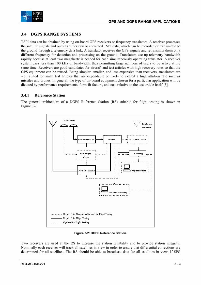
GPS AND DGPS RANGE APPLICATIONS

RTO-AG-160-V21 3 - 3

3.4 DGPS RANGE SYSTEMS

TSPI data can be obtained by using on-board GPS receivers or frequency translators. A receiver processes the satellite signals and outputs either raw or corrected TSPI data, which can be recorded or transmitted to the ground through a telemetry data link. A translator receives the GPS signals and retransmits them on a different frequency for detection and processing on the ground. Translators use up telemetry bandwidth rapidly because at least two megahertz is needed for each simultaneously operating translator. A receiver system uses less than 100 kHz of bandwidth, thus permitting large numbers of users to be active at the same time. Receivers are good candidates for aircraft and test articles with high recovery rates so that the GPS equipment can be reused. Being simpler, smaller, and less expensive than receivers, translators are well suited for small test articles that are expendable or likely to exhibit a high attrition rate such as missiles and drones. In general, the type of on-board equipment chosen for a particular application will be dictated by performance requirements, form-fit factors, and cost relative to the test article itself [5].

3.4.1 Reference Station The general architecture of a DGPS Reference Station (RS) suitable for flight testing is shown in Figure 3-2.

Figure 3-2: DGPS Reference Station.

Two receivers are used at the RS to increase the station reliability and to provide station integrity. Nominally each receiver will track all satellites in view in order to assure that differential corrections are determined for all satellites. The RS should be able to broadcast data for all satellites in view. If SPS

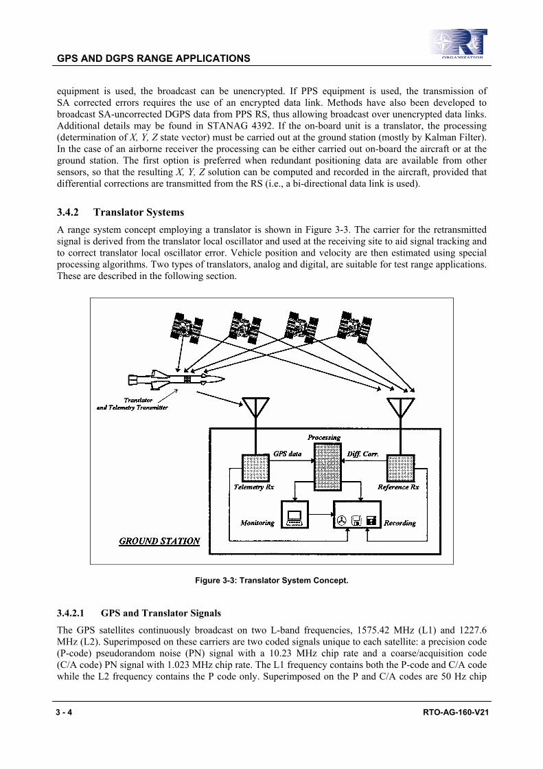
GPS AND DGPS RANGE APPLICATIONS

3 - 4 RTO-AG-160-V21

equipment is used, the broadcast can be unencrypted. If PPS equipment is used, the transmission of SA corrected errors requires the use of an encrypted data link. Methods have also been developed to broadcast SA-uncorrected DGPS data from PPS RS, thus allowing broadcast over unencrypted data links. Additional details may be found in STANAG 4392. If the on-board unit is a translator, the processing (determination of X, Y, Z state vector) must be carried out at the ground station (mostly by Kalman Filter). In the case of an airborne receiver the processing can be either carried out on-board the aircraft or at the ground station. The first option is preferred when redundant positioning data are available from other sensors, so that the resulting X, Y, Z solution can be computed and recorded in the aircraft, provided that differential corrections are transmitted from the RS (i.e., a bi-directional data link is used).

3.4.2 Translator Systems A range system concept employing a translator is shown in Figure 3-3. The carrier for the retransmitted signal is derived from the translator local oscillator and used at the receiving site to aid signal tracking and to correct translator local oscillator error. Vehicle position and velocity are then estimated using special processing algorithms. Two types of translators, analog and digital, are suitable for test range applications. These are described in the following section.

Figure 3-3: Translator System Concept.

3.4.2.1 GPS and Translator Signals

The GPS satellites continuously broadcast on two L-band frequencies, 1575.42 MHz (L1) and 1227.6 MHz (L2). Superimposed on these carriers are two coded signals unique to each satellite: a precision code (P-code) pseudorandom noise (PN) signal with a 10.23 MHz chip rate and a coarse/acquisition code (C/A code) PN signal with 1.023 MHz chip rate. The L1 frequency contains both the P-code and C/A code while the L2 frequency contains the P code only. Superimposed on the P and C/A codes are 50 Hz chip

GPS AND DGPS RANGE APPLICATIONS

RTO-AG-160-V21 3 - 5

rate navigation data containing the ‘navigation message’ (see Annex A for more detailed information about GPS signal structure). A typical receive level in a 1.5 MHz bandwidth for the L1 C/A signal at a ground station is -160 dBW from a 0 dBi antenna. When a translator is employed, the GPS signals are degraded by the translation process and by sidebands on the output carrier which may induce noise at the receiver input. The transmitted signal-to-noise ratio, S N t , may be expressed as [6]:

S N S NN Nt sr= ⋅

⋅

1 1

1 2 (3.1)

where:

S N sr = translator received signal-to-noise ratio;

N1 = degradation due to the translation process; and

N2 = receive system degradation due to transmitter induced noise.

Accurate trajectory measurements can be obtained even when S N t is as low as – 30 dB in a 1.5 MHz bandwidth since there is a recovery of 40 dB or more after the signals are despread.

The output spectrum of a translator can be characterised as band-limited noise so that the signal-to-noise ratio at the remote acquisition site, S N sr , is:

+

=NR

Rtsr PP

PNSNS (3.2)

where:

PR = power of the translated signal at the receiving system input; and

PN = receiving system noise power referenced to the receiver input.

3.4.2.2 Analog and Digital Translators

Both analog and digital translators commonly operate with the L1 C/A signals. The analog translator simply receives the satellite signals and retransmits them on another frequency. The first generation analog translator used conventional heterodyne techniques and class A amplification to ensure that nonlinearities did not introduce phase noise on the satellite signals. A second generation miniaturised analog translator has been developed using limiting and class C amplification to reduce power requirements [6].

The digital translator is applicable to situations where the transmitted data must be encrypted or when telemetry and GPS signals are to be simultaneously relayed on the same link. However, the digital translator requires higher transmitted power than the analog translator for equivalent performance.

When analog or digital translator signals are transmitted at S-band, standard telemetry equipment at many test ranges can be used. The S-band signals can be received and down-converted to a suitable record frequency, and possibly wideband recorded and played back when a proper Time Base Error Corrector (TBEC) is employed. Field test results indicate TBEC equipment may reduce standard recorder time base error sufficiently to allow GPS receiver lockup during playback using conventional 4 MHz telemetry recorders. The acquisition site and the central processing site on the ground may not to be collocated. Minimum acquisition site equipment (telemetry receiver, local oscillator error correction, etc.) is needed when data are relayed for processing at a central facility. When an acquisition site is configured with a GPS

GPS AND DGPS RANGE APPLICATIONS

3 - 6 RTO-AG-160-V21

receiver for processing translator signals, a GPS reference receiver, and common frequency and time references, trajectory estimation may be feasible even using data from only three satellites. The advantages of using a translator (analog or digital) are:

• It is less complex than a GPS receiver, which can reduce cost, size, and weight of this component up to an order of magnitude;

• It shifts the computational capability to ground base, thus allowing this capability to increase, and enabling Time-to-first-fix (TTFF) of typically less than 5 seconds for range safety applications;

• It allows mission replay, and it gives the system inherent differential GPS accuracy; and

• It allows tracking under very high g-levels.

There are also some disadvantages when using translators, but they are not a factor for many applications; these disadvantages are:

• Only a limited number of targets can be tracked simultaneously because of translator retransmission bandwidth requirements;

• TSPI is not directly available for use by the vehicle; and

• Recording on-board the vehicle is typically impossible, making a line-of-sight relationship to the master station mandatory (i.e., if loss of satellite signal track or masking of the GPS/Telemetry antennae occurs, position data will be totally lost).

Over the last fifteen years many translators have been built and tested and new processing techniques are now being investigated to increase the performance of existing equipment at the ranges. More information about GPS translators and techniques for receiving, processing, and recording translated GPS signals using standard telemetry equipment can be found in the literature [6, 7].

3.4.3 Airborne Receivers The airborne GPS receiver can be either podded or installed in the aircraft avionics compartment. In both cases the same concept applies. There are many possible configurations for both the on-board/podded equipment and the Reference Station with supporting test facilities on the ground. Airborne and ground equipment selection criteria are mainly dictated by the task of the test mission and cost-vs.-accuracy considerations.

A possible layout is shown in Figure 3-4. The on-board GPS receiver together with the other data sensors and equipment carried on the aircraft for recording information, processing and transmitting/receiving data are commonly referred to as the airborne Flight Test Instrumentation (FTI).

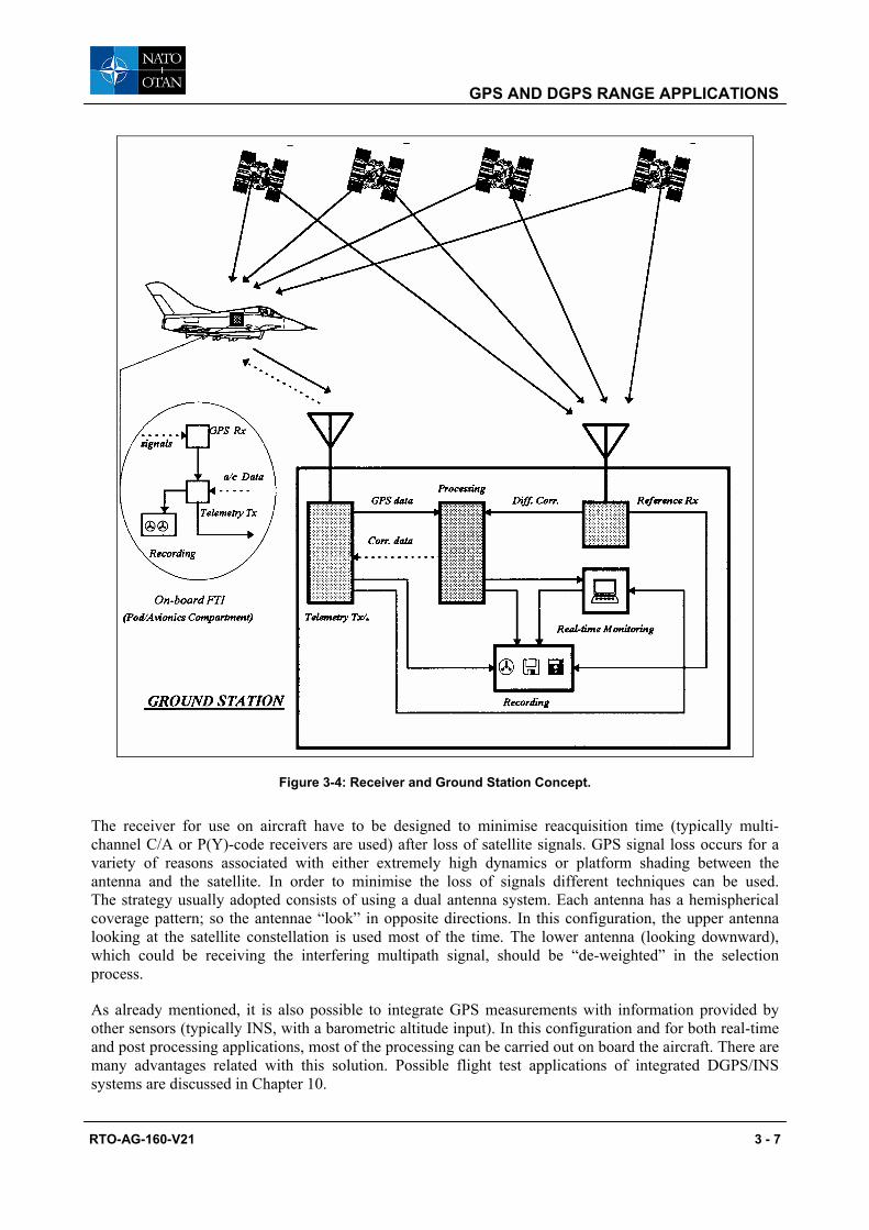
GPS AND DGPS RANGE APPLICATIONS

RTO-AG-160-V21 3 - 7

Figure 3-4: Receiver and Ground Station Concept.

The receiver for use on aircraft have to be designed to minimise reacquisition time (typically multi-channel C/A or P(Y)-code receivers are used) after loss of satellite signals. GPS signal loss occurs for a variety of reasons associated with either extremely high dynamics or platform shading between the antenna and the satellite. In order to minimise the loss of signals different techniques can be used. The strategy usually adopted consists of using a dual antenna system. Each antenna has a hemispherical coverage pattern; so the antennae “look” in opposite directions. In this configuration, the upper antenna looking at the satellite constellation is used most of the time. The lower antenna (looking downward), which could be receiving the interfering multipath signal, should be “de-weighted” in the selection process.

As already mentioned, it is also possible to integrate GPS measurements with information provided by other sensors (typically INS, with a barometric altitude input). In this configuration and for both real-time and post processing applications, most of the processing can be carried out on board the aircraft. There are many advantages related with this solution. Possible flight test applications of integrated DGPS/INS systems are discussed in Chapter 10.

GPS AND DGPS RANGE APPLICATIONS

3 - 8 RTO-AG-160-V21

3.5 REFERENCES

[1] Riley, S. and Daly, P. (1993). “Performance of the GLONASS P-code at L1 and L2 Frequencies”. American Institute of Navigation (ION) – Satellite Division. Proceedings of the 6th International Technical Meeting.

[2] Ochieng, W.Y. (1997). “GNSS Design”. MSc Lecture Notes. Institute of Engineering Surveying and Space Geodesy (IESSG) – University of Nottingham (UK).

[3] Kayton, M. and Fried, W.R. (1997). “Avionics Navigation Systems”. Second Edition. John Wiley & Sons (USA).

[4] Joint Program Office (JPO). (1991). “NAVSTAR GPS User Equipment, Introduction”. Public Release Version. US Air Force Space Systems Division, NAVSTAR-GPS Joint Program Office (JPO). Los Angeles AFB, California (USA).

[5] Parkinson, B.W. and Spilker, J.J., Jr. Editors. (1996). “Global Positioning System: Theory and Applications – Volume II”. Progress in Astronautics and Aeronautics. Vol. 163. Published by the American Institute of Aeronautics and Astronautics.

[6] McConnell, J.B., Greenberg, R.H. and Pickett, R.B. (1989). “Advances in GPS Translator Technology”. American Institute of Navigation (ION) – Satellite Division. Proceedings of the 2nd International Technical Meeting.

[7] Brown, A.K. (1992). “Test Results of the Advanced Translator Processing System”. NAVSYS Corporation Technical Paper, Colorado Springs (CO), USA.

RTO-AG-160-V21 4 - 1

Chapter 4 – DGPS REQUIREMENTS AND EQUIPMENT SELECTION

4.1 INTRODUCTION

As discussed in the previous chapters, accurate determination of aircraft position is a strong requirement in several flight test applications and often requires a significant effort in terms of availability of test ranges properly instrumented with optical or radar tracking systems, time for data reduction and dependency on environmental and meteorological conditions.

The foreseen capabilities of GPS, in terms of data accuracy, quickness of data availability and reduction of cost, moved many military and civilian flight test organizations to consider DGPS-TSPI systems. Most efforts are addressed to GPS using C/A code, with post-flight differentiation. This is usually preferred to GPS using P-code due to both simplicity of use and high accuracy attainable notwithstanding its lower cost. In the following discussion of DGPS-TSPI systems requirements, we will mostly refer to fast jets applications.

4.2 DGPS TECHNICAL REQUIREMENTS

In general, a DGPS-TSPI system has to include the following elements:

• A GPS receiver with differential capability to be installed in the aircraft;

• A ground Reference Station (RS); and

• The software for computation of the correction parameters.

The corrections computed in the RS should be applicable to the Airborne Receiver (AR) data in post-processing or, optionally, in real-time.

All systems have to be designed in accordance with the following military standards:

• MIL-STD-461, for identification of electromagnetic emissions and control of the interference;

• MIL-STD-462, for evaluation and measurement methodology of electromagnetic interference;

• MIL-STD-704, referring to airborne electric power generation systems; and

• MIL-STD-810, relative to the different methods for evaluating environmental factors affecting the performance of electronic systems (temperature, humidity, vibrations, etc.).

4.2.1 Airborne Receiver The on board receiver (L1 frequency, C/A code receiver) should have at least 9 channels. Optionally, the system would also be able to operate with both L1 and L2 frequencies (P-code) or process carrier phases. The ability to program the receiver, before flight, directly with the system control-display unit or with a common PC is required. As a minimum, the following three parameters should be inserted (on the ground) for selection of the best satellite constellation:

• PDOP Threshold (PT). Corresponding to the minimum PDOP for positioning computation;

• Minimum Elevation Angle (MEA). This parameter represents the minimum elevation of satellites over the horizon for inclusion in the positioning computation; and

• Signal-to-Noise Ratio (SNR). This parameter represents the intensity of the satellite signals with respect to noise. A low SNR has a negative effect on code acquisition.

DGPS REQUIREMENTS AND EQUIPMENT SELECTION

4 - 2 RTO-AG-160-V21

Moreover, the satellites should be automatically selected in order to obtain the best PDOP factor or, alternatively, the satellites to be included in the positioning computation should be selectable by the operator at the ground programming stage.

The airborne system has to be able to operate in both stand-alone and differential modes, and to provide position and velocity in two and three dimensions (with or without height data). Optionally, the system could be aided with a barometric altimeter or an inertial navigation system.

The dynamic conditions in which the sensor should operate are the following:

• Maximum speed: 800 kts;

• Acceleration: ≥ 4 g; and

• Jerk: ≥ 2 g/s.

The accuracies of position and velocity data, with and without Selective Availability, have to be:

• Stand-Alone Mode (non-differential).

• Without SA: Position: 25 m SEP; Velocity: 0.02 m/s RMS.

• With SA: Position: 100 m 2d-RMS; Velocity: 0.1 m/s RMS.

• Real-Time Differential Mode.

• With or without SA: Position: 10 m SEP; Velocity: 0.02 m/s RMS.

• Post-Processing Differential Mode.

• With or without SA: Position: 5 m SEP; Velocity: 0.02 m/s RMS.

Once turned-on the on-board receiver has to be able to give TSPI after not more than 2 minutes (Time To First Fix – TTFF). If the receiver has been already initialised with external positioning data, the information has to be provided within 1 minute (Reaction Time – REAC).

Time, position and velocity data have to be available from the receiver at a minimum rate of 1 Hz (1 data/sec) and preferably up to 20 Hz (this data rate is sufficient for most applications, although data rates of up to 300 Hz can be required in very high dynamics applications). The transmission of data from the sensor to the other on-board systems (magnetic recorder, differential processing unit, etc.) can be made with a standard RS-422/RS-232 interface and/or with ARINC-429, MIL-STD-1553, USB, etc.

The system should be able to conform to the RTCM-SC-104 standard protocol for differential corrections.

The antenna can be either a standard Fixed Radiation Pattern Antenna (FRPA) with a pre-amplification and filtering unit, or a Controlled Radiation Pattern Antenna (CRPA) with relative control unit.

4.2.2 Ground Receiver The minimum requirement for the GPS system in the ground RS is for an L1, C/A code receiver with 9 parallel channels. Optionally, the system would also operate with both L1 and L2 frequencies (P code),

DGPS REQUIREMENTS AND EQUIPMENT SELECTION

RTO-AG-160-V21 4 - 3

use carrier phase or combinations of pseudoranges and carrier phases. The system has to be able to provide the differential correction parameters using the RTCM-SC-104 standard protocol and to record satellite data for at list 4 hours. Finally, the system should be equipped with a control-display unit or should be linkable to a generic PC keyboard/screen.

4.2.3 Software The system software has to perform the following functions:

• Provide the three-dimensional position of the aircraft (in WGS84 co-ordinates) at a frequency of 1 – 10 Hz , with an accuracy of 5 m SEP;

• Provide, with an accuracy of 0.02 m/s RMS, the velocity along the three axes of the aircraft at a rate of 1 Hz (minimum); and

• Provide UTC time.

These data have to be computed by the software and made readily available to the operator, based on the following input data:

• On-board GPS receiver data; and

• Ground GPS receiver data and differential corrections.

4.3 EQUIPMENT SELECTION

A large variety of GPS receivers are available on the commercial market, which can be used for DGPS applications. Particularly, two classes of receivers are well suited for flight test applications:

• Surveying GPS receivers; and

• Aviation GPS receivers.

The two options are briefly discussed in the following paragraphs.

4.3.1 Surveying Products Surveying, in requiring accurate and repeatable results, is currently one of the most demanding GPS applications. It is a common practice to employ a survey type receiver for the remote station, and an aviation receiver for the aircraft mounted receiver (but this is certainly not the only option!).

GPS surveying products enable operators to achieve centimetre or even millimetre levels of accuracy. Selection of GPS receivers belonging to survey class (both for ground station and aircraft installations) should take into account, more than in standard surveying applications, factors like power consumption, antenna requirements, operating temperature range, resistance to humidity, load factor, etc. An advantage is that virtually all commercially available surveying receivers are already designed for DGPS operations (generally in post-processing or on-the-fly). Examples of GPS receivers belonging to this class are the TRIMBLE 4000SE/SSE, the ASHTECH Z-12, the NovAtel ProPak and the SOKKIA GSR2100. All these receivers are multi-channel (up to 12 channels) with all-in-view capability. These types of receivers are well suited for flight test applications because they are capable of tracking both pseudorange and carrier phase observables, both on the L1 and L2 frequencies (mostly adopting cross-correlation techniques), thereby providing centimetre level accuracies on-the-fly or even millimetre accuracies in post-processing applications.

The majority of current receivers also adopt the ASHTECH patented Z-Technology. This is the process for mitigating or eliminating the effects of DoD Anti-Spoofing (A-S) and thereby retaining receiver lock

DGPS REQUIREMENTS AND EQUIPMENT SELECTION

4 - 4 RTO-AG-160-V21

and tracking capability at all times for those satellites in view. This technique separately matches the Y-Code on the L1 and L2 frequencies against a different, locally generated P-Code; in essence it is a correlation process that recaptures the encryption code on each signal. Since each carrier contains the encryption code, with sufficient signal integration the encryption bits can be estimated for signals on both the L1 and L2 bands. Each signal is compared to the other, so the encryption code can be removed. After this has been accomplished, it can be measured. Z-Technology receivers are capable of tracking rapidly varying ionosphere with full observable accuracy. This cannot be accomplished with standard cross correlation receivers. Acquisition transients settle in seconds, while the majority of other systems have to wait minutes before the A-S observables reach equivalent accuracy [1].

A good example of a surveying GPS receiver suitable for flight test applications is the ASHTECH Z-12. This is a 12 channel receiver which can automatically track the GPS satellites following the indications given by the user (by means of a keyboard and a display) in terms of minimum elevation angle (for multipath reduction) and minimum number of satellites for position calculation. The expected accuracy of the system varies between 10 and 100 m SEP depending on SA, but this is significantly improved using differential corrections. The keyboard and the display are located on the receiver front panel, while the input/output connections are located on the back (Figure 4-1).

Receiver front panel Receiver back panel

Figure 4-1: ASHTECH XII/Z-12 GPS Receiver.

On the back panel there are connections for the antenna, for a photogrammetric camera, for external time and frequency synchronization, the serial ports through which data can be transferred to a personal computer, a magnetic tape or the telemetry system, and a humidity sensor. The receiver can operate with a voltage between 10 and 32 Vdc, which can be provided by two external batteries linked to separate connectors. If one of the two batteries gets flat, the luck of voltage (less than 10 Vdc) is displayed and the other battery automatically becomes operative without interruption of data recording [1].

The ASHTECH Z-12 automatically switches to Z-tracking when anti-spoofing is employed. If A-S were implemented in the event that a conflict arose involving the U.S. military, centimetre accurate measurements would still be possible anywhere in the world. With the Z-tracking technology, there would be virtually no degradation in measurement accuracy.

An antenna that can be used with the ASHTECH Z-12 receiver is shown in Figure 4-2. This is a micro-strip antenna that can be mounted on a precisely adjustable platform and protected with an impermeable cover.

DGPS REQUIREMENTS AND EQUIPMENT SELECTION

RTO-AG-160-V21 4 - 5

Figure 4-2: ASHTECH Antenna Platform (Mod. GPS S67-1575-S).

This particular antenna is designed to operate at the L1 frequency (1575.42 MHz). Its radiation pattern is shown in Figure 4-2. The main characteristics of the ASHTECH GPS antenna are listed in Table 4-1.

Table 4-1: ASHTECH Antenna Characteristics (Mod. GPS S67-1575-S)

ELECTRICAL MECHANICAL ENVIRONMENTAL

Frequency: 1575.42 Mhz VSWR: 1.5:1 Polarization: RHCP Impedance: 50 ohms Power Required: 1 watt Gain: – 1.0 dB 0° ≤ φ < 75°

– 2.5 dB 75°≤ φ < 80° – 4.5 dB 80°≤ φ < 85° – 7.5 dB φ = 90° @ Horizon

Weight: 3 oz. Thickness: 0.404 in. Diameter: 3.5 in. Material: Aluminium 6061 – T61 /

Plastic Cover Connector: TNC

Temperature: – 67 °F ÷ 185 °F Vibrations: 10 Gs Height: 55000 ft

4.3.2 Aviation Products Some standard aviation GPS receivers can be also used well for flight test applications, but in this case it is essential to select products with DGPS capability (either embedded or external). This can be achieved either in post-processing or in real-time (usually using a radio link compliant with the RTCM/RTCA standard formats).

For example, the TRIMBLE 8100 aviation receiver is an advanced airborne navigation system designed for the current and likely future needs of civilian and military aircraft operations. It is an advanced device

DGPS REQUIREMENTS AND EQUIPMENT SELECTION

4 - 6 RTO-AG-160-V21

with a host of features designed to enable seamless transition between all phases of flight navigation (i.e., oceanic, en route, terminal and non-precision approach). The 8100 receiver can operate as a standalone device or can interface via a data terminal with a variety of sensors that input information to an aircraft guidance system. This is a 9-channel receiver, easily upgradeable to 12-channel operation and, when it becomes necessary, to meet the WAAS specification. TRIMBLE 8100 supports FANS concepts to replace navigation information now provided by VOR, INS, DME, and OMEGA systems, and it is DGPS capable, in anticipation of future Category I, II and III approach and landing certifications [2].

ASHTECH also developed a 12-channel all-in-view receiver with Z-Technology suitable for aircraft installation. This system, named ASHTECH X-Treme, can be used in flight applications requiring accurate trajectory measurement data, such as airborne photogrammetry and flight-testing [3].

A good combination could be also using a standard 12-channel all-in-view geodetic receiver for the DGPS ground station (e.g., TRIMBLE 4000 SSE or ASHTECH Z-12), and an airborne receiver with embedded or external data recording capability (e.g., TRIMBLE 8100, ASHTECH X-Treme).

4.4 REFERENCES

[1] ASHTECH Inc. (2001). “ASHTECH Z-12 Receiver”. Technical Specification Leaflet.

[2] TRIMBLE Navigation Inc. (2001). “TRIMBLE 8100 Airborne GPS Navigation System”. Technical Specification Leaflet.

[3] ASHTECH Inc. (2005). “ASHTECH X-Treme Receiver”. Technical Specification Leaflet.

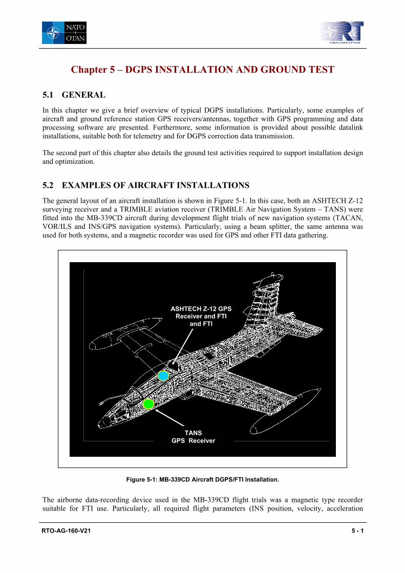
RTO-AG-160-V21 5 - 1

Chapter 5 – DGPS INSTALLATION AND GROUND TEST

5.1 GENERAL

In this chapter we give a brief overview of typical DGPS installations. Particularly, some examples of aircraft and ground reference station GPS receivers/antennas, together with GPS programming and data processing software are presented. Furthermore, some information is provided about possible datalink installations, suitable both for telemetry and for DGPS correction data transmission.

The second part of this chapter also details the ground test activities required to support installation design and optimization.

5.2 EXAMPLES OF AIRCRAFT INSTALLATIONS

The general layout of an aircraft installation is shown in Figure 5-1. In this case, both an ASHTECH Z-12 surveying receiver and a TRIMBLE aviation receiver (TRIMBLE Air Navigation System – TANS) were fitted into the MB-339CD aircraft during development flight trials of new navigation systems (TACAN, VOR/ILS and INS/GPS navigation systems). Particularly, using a beam splitter, the same antenna was used for both systems, and a magnetic recorder was used for GPS and other FTI data gathering.

TANS GPS Receiver

ASHTECH Z-12 GPSReceiver and FTI

and FTI

Figure 5-1: MB-339CD Aircraft DGPS/FTI Installation.

The airborne data-recording device used in the MB-339CD flight trials was a magnetic type recorder suitable for FTI use. Particularly, all required flight parameters (INS position, velocity, acceleration

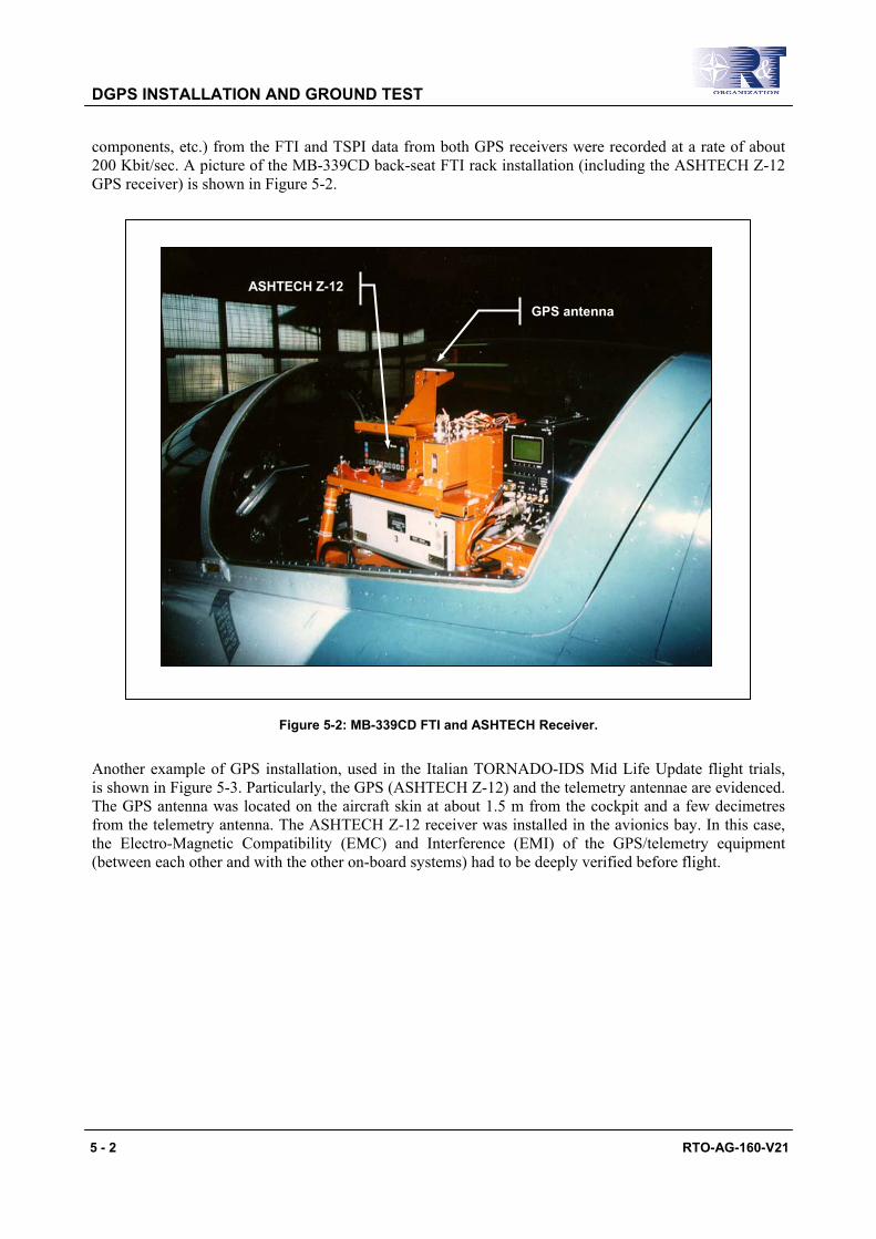
DGPS INSTALLATION AND GROUND TEST

5 - 2 RTO-AG-160-V21

components, etc.) from the FTI and TSPI data from both GPS receivers were recorded at a rate of about 200 Kbit/sec. A picture of the MB-339CD back-seat FTI rack installation (including the ASHTECH Z-12 GPS receiver) is shown in Figure 5-2.

ASHTECH Z-12

GPS antenna

Figure 5-2: MB-339CD FTI and ASHTECH Receiver.

Another example of GPS installation, used in the Italian TORNADO-IDS Mid Life Update flight trials, is shown in Figure 5-3. Particularly, the GPS (ASHTECH Z-12) and the telemetry antennae are evidenced. The GPS antenna was located on the aircraft skin at about 1.5 m from the cockpit and a few decimetres from the telemetry antenna. The ASHTECH Z-12 receiver was installed in the avionics bay. In this case, the Electro-Magnetic Compatibility (EMC) and Interference (EMI) of the GPS/telemetry equipment (between each other and with the other on-board systems) had to be deeply verified before flight.

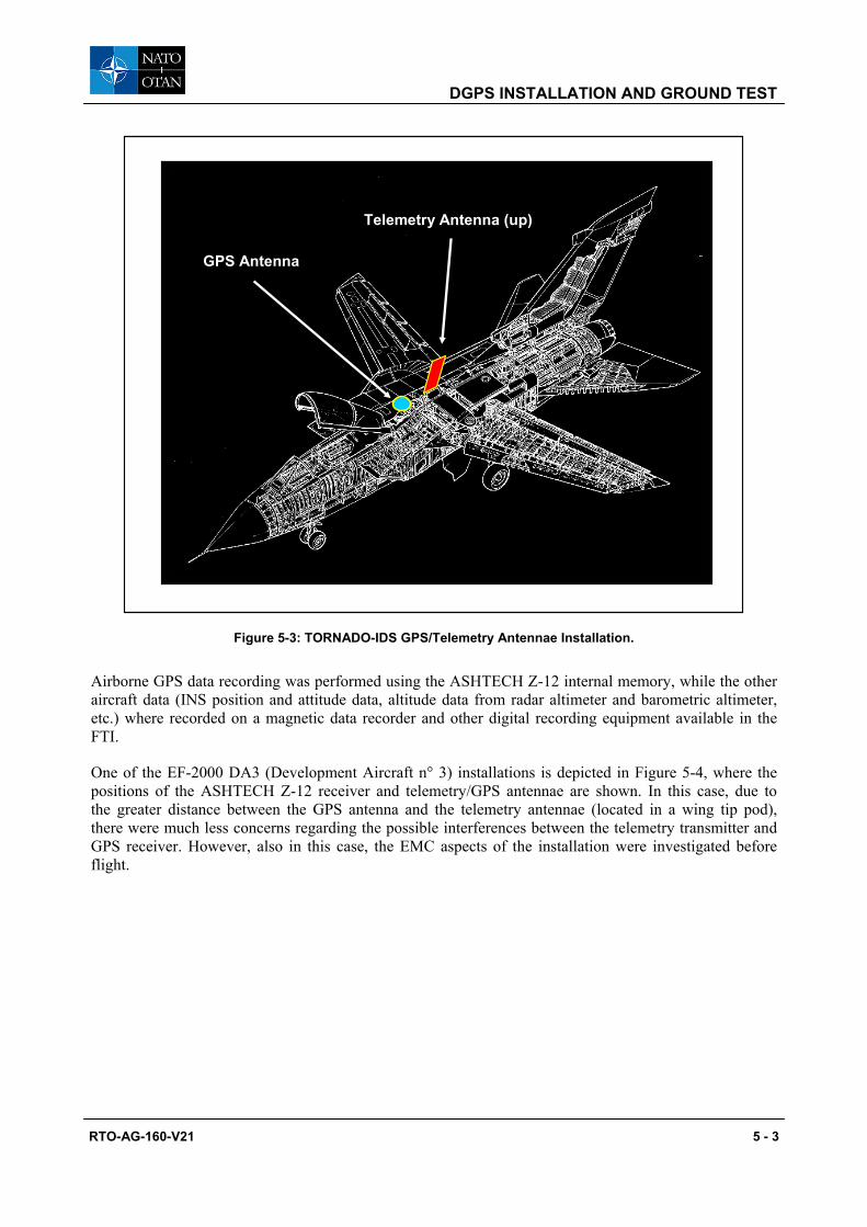
DGPS INSTALLATION AND GROUND TEST

RTO-AG-160-V21 5 - 3

GPS Antenna

Telemetry Antenna (up)

Figure 5-3: TORNADO-IDS GPS/Telemetry Antennae Installation.

Airborne GPS data recording was performed using the ASHTECH Z-12 internal memory, while the other aircraft data (INS position and attitude data, altitude data from radar altimeter and barometric altimeter, etc.) where recorded on a magnetic data recorder and other digital recording equipment available in the FTI.

One of the EF-2000 DA3 (Development Aircraft n° 3) installations is depicted in Figure 5-4, where the positions of the ASHTECH Z-12 receiver and telemetry/GPS antennae are shown. In this case, due to the greater distance between the GPS antenna and the telemetry antennae (located in a wing tip pod), there were much less concerns regarding the possible interferences between the telemetry transmitter and GPS receiver. However, also in this case, the EMC aspects of the installation were investigated before flight.

DGPS INSTALLATION AND GROUND TEST

5 - 4 RTO-AG-160-V21

GPS antenna

Telemetry GPS receiver

Figure 5-4: EF-2000 GPS/Telemetry Installation.

5.3 GPS SYSTEMS SET-UP

Before performing flight trials, it is important to select the set-up parameters of the on-board GPS receiver. These parameters can be programmed either by using the GPS receiver control panel units (e.g., ASHTECH Z-12 keyboard/display [1] on the receiver front panel) or by using a remote programming unit (e.g., a common PC in the case of TANS). Optimal parameters for flight test TSPI applications are the following:

• Data recording rate: 1 – 10 samples/sec;

• Masking angle: 10° (i.e., minimum satellite elevation over the horizon for multipath reduction);

• Minimum number of satellites for position computation: 3 only when using an external accurate altitude input (not with last available GPS altitude data) – 4 in all other cases1;

• PDOP threshold (for position calculation): less than 5; and

• Minimum satellite signal SNR: 15 – 30 dB.

5.4 GPS DATA DOWNLOADING AND PROCESSING

As discussed in Chapter 3, GPS data downloading (from both the on-board and ground reference receivers) and differential processing can be performed on the ground (post-flight) for accurate aircraft trajectory reconstruction. In other cases (real-time DGPS implementations with datalink) differentially corrected data are computed on the ground by the reference station (one-way link) or in flight (bi-directional link), and recorded on-board the aircraft. In most practical implementations, however, the post-processing option is preferred both due to simplicity and high accuracy attainable with off-line carrier phase processing. In the following, some representative information is given about some of the ASHTECH post-flight data downloading and processing options. Particularly, the data transfer and differential processing procedures used with the ASHTECH Z-12 receivers (including a description of the relevant data files formats) is given in the following paragraphs, together with examples of dedicated

1 Some GPS receivers incorporate an option that allows calculation of position using measurements from only 3 satellites (in this case, as tracking to the fourth satellite is lost, the last calculated height data is used to provide a position solution). In this case, obviously, the accuracy may degrade significantly in case of sudden aircraft altitude variations.

DGPS INSTALLATION AND GROUND TEST

RTO-AG-160-V21 5 - 5

Flight Test Data Analysis (FTDA) software tools developed for the TORNADO-IDS and EF-2000 flight trials.

5.4.1 ASHTECH Data Downloading Data downloading from the ASHTECH Z-12 receiver can be performed using the P-NAV software package, running on a common PC [1, 2]. Data are transferred to the PC through one of the available serial ports, using an RS-232-C standard interface.

The ASHTECH receiver can store data in different formats depending on the user requirements. Particularly, the receiver can:

• Store raw data (pseudorange and carrier phase) and position information (B-file in binary format), which can be corrected via software in post-processing using ephemeris data (E-file or ephemeris file) or in real-time;

• Store only raw (pseudorange and carrier phase) measurement data (B-file), which can be differentiated post-flight and ephemeris data (E-file). Position is calculated during data transfer; and

• Store position data in ASCII format (C-file) which can be corrected only in real-time.

During the TORNADO-IDS/EF-2000 trials, the first option was adopted. Therefore, the files gathered from the ASHTECH receiver, in binary format, are the B-files (code and carrier phases raw data, position calculated for each epoch and measurement quality parameters), the E-files (ephemeris parameters and satellite clock corrections) and, in ASCII format, the S-files (measurement site identifier, antenna height, meteorological information, and receiver type).

Differential processing (pseudorange) is carried out using a Post Processing Differentiation (PPDIFF) program, by simply inserting the coordinates of the reference station (previously determined by surveying). The computer then calculates the correction by simply subtracting true ranges from measured ranges. Corrections are then applied to the measurements of the on-board receiver (B-files).

Obviously, the externally inserted data have to be compatible with the B-file format, and therefore must include latitude, longitude, height (λ, φ, h) or cartesian coordinates (X, Y, Z) in WGS-84. The result of the differential processing carried out with the PPDIFF is a data file in ASCII format, conventionally named C-file (Figure 5-5).

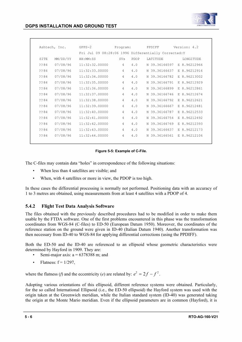
DGPS INSTALLATION AND GROUND TEST

5 - 6 RTO-AG-160-V21

Ashtech, Inc. GPPS-2 Program: PPDIFF Version: 4.2

Fri Jul 09 08:28:06 1996 Differentially Corrected:Y

SITE MM/DD/YY HH:MM:SS SVs PDOP LATITUDE LONGITUDE

??84 07/08/96 11:32:32.00000 4 4.0 N 39.36166597 E 8.96212966

??84 07/08/96 11:32:33.00000 4 4.0 N 39.36166637 E 8.96212916

??84 07/08/96 11:32:34.00000 4 4.0 N 39.36166782 E 8.96213002

??84 07/08/96 11:32:35.00000 4 4.0 N 39.36166791 E 8.96212929

??84 07/08/96 11:32:36.00000 4 4.0 N 39.36166899 E 8.96212861

??84 07/08/96 11:32:37.00000 4 4.0 N 39.36166746 E 8.96212674

??84 07/08/96 11:32:38.00000 4 4.0 N 39.36166792 E 8.96212621

??84 07/08/96 11:32:39.00000 4 4.0 N 39.36166667 E 8.96212481

??84 07/08/96 11:32:40.00000 4 4.0 N 39.36166787 E 8.96212533

??84 07/08/96 11:32:41.00000 4 4.0 N 39.36166754 E 8.96212492

??84 07/08/96 11:32:42.00000 4 4.0 N 39.36166769 E 8.96212393

??84 07/08/96 11:32:43.00000 4 4.0 N 39.36166637 E 8.96212173

??84 07/08/96 11:32:44.00000 4 4.0 N 39.36166561 E 8.96212106

Figure 5-5: Example of C-File.

The C-files may contain data “holes” in correspondence of the following situations:

• When less than 4 satellites are visible; and

• When, with 4 satellites or more in view, the PDOP is too high.

In these cases the differential processing is normally not performed. Positioning data with an accuracy of 1 to 3 metres are obtained, using measurements from at least 4 satellites with a PDOP of 4.

5.4.2 Flight Test Data Analysis Software The files obtained with the previously described procedures had to be modified in order to make them usable by the FTDA software. One of the first problems encountered in this phase was the transformation coordinates from WGS-84 (C-files) to ED-50 (European Datum 1950). Moreover, the coordinates of the reference station on the ground were given in ID-40 (Italian Datum 1940). Another transformation was then necessary from ID-40 to WGS-84 for applying differential corrections (using the PPDIFF).

Both the ED-50 and the ID-40 are referenced to an ellipsoid whose geometric characteristics were determined by Hayford in 1909. They are:

• Semi-major axis: a = 6378388 m; and

• Flatness: f = 1/297,

where the flatness (f) and the eccentricity (e) are related by: e f f2 22= − .

Adopting various orientations of this ellipsoid, different reference systems were obtained. Particularly, for the so called International Ellipsoid (i.e., the ED-50 ellipsoid) the Hayford system was used with the origin taken at the Greenwich meridian, while the Italian standard system (ID-40) was generated taking the origin at the Monte Mario meridian. Even if the ellipsoid parameters are in common (Hayford), it is

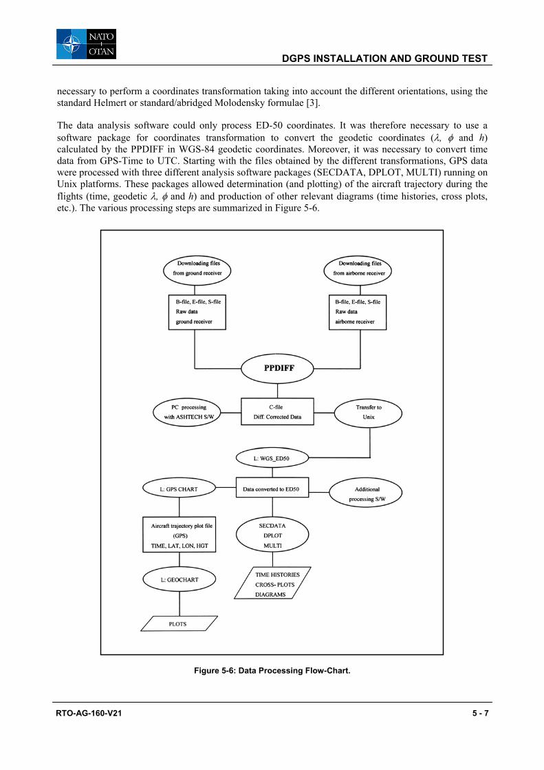
DGPS INSTALLATION AND GROUND TEST

RTO-AG-160-V21 5 - 7

necessary to perform a coordinates transformation taking into account the different orientations, using the standard Helmert or standard/abridged Molodensky formulae [3].

The data analysis software could only process ED-50 coordinates. It was therefore necessary to use a software package for coordinates transformation to convert the geodetic coordinates (λ, φ and h) calculated by the PPDIFF in WGS-84 geodetic coordinates. Moreover, it was necessary to convert time data from GPS-Time to UTC. Starting with the files obtained by the different transformations, GPS data were processed with three different analysis software packages (SECDATA, DPLOT, MULTI) running on Unix platforms. These packages allowed determination (and plotting) of the aircraft trajectory during the flights (time, geodetic λ, φ and h) and production of other relevant diagrams (time histories, cross plots, etc.). The various processing steps are summarized in Figure 5-6.

Figure 5-6: Data Processing Flow-Chart.

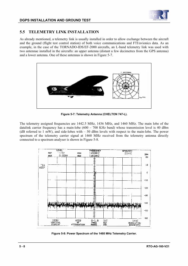
DGPS INSTALLATION AND GROUND TEST

5 - 8 RTO-AG-160-V21

5.5 TELEMETRY LINK INSTALLATION

As already mentioned, a telemetry link is usually installed in order to allow exchange between the aircraft and the ground (flight test control station) of both voice communications and FTI/avionics data. As an example, in the case of the TORNADO-IDS/EF-2000 aircrafts, an L-band telemetry link was used with two antennae installed in the aircrafts: an upper antenna (distant a few decimetres from the GPS antenna) and a lower antenna. One of these antennas is shown in Figure 5-7.

Figure 5-7: Telemetry Antenna (CHELTON 747-L).

The telemetry assigned frequencies are 1442.5 MHz, 1436 MHz, and 1460 MHz. The main lobe of the datalink carrier frequency has a main-lobe (600 – 700 KHz band) whose transmission level is 40 dBm (dB referred to 1 mW), and side-lobes with – 50 dBm levels with respect to the main-lobe. The power spectrum of the telemetry carrier signal at 1460 MHz received from the telemetry antenna directly connected to a spectrum analyser is shown in Figure 5-8.

Figure 5-8: Power Spectrum of the 1460 MHz Telemetry Carrier.

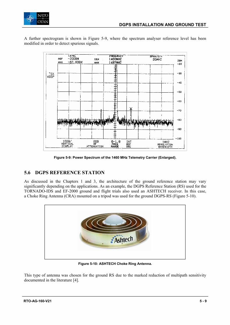
DGPS INSTALLATION AND GROUND TEST

RTO-AG-160-V21 5 - 9

A further spectrogram is shown in Figure 5-9, where the spectrum analyser reference level has been modified in order to detect spurious signals.

Figure 5-9: Power Spectrum of the 1460 MHz Telemetry Carrier (Enlarged).

5.6 DGPS REFERENCE STATION

As discussed in the Chapters 1 and 3, the architecture of the ground reference station may vary significantly depending on the applications. As an example, the DGPS Reference Station (RS) used for the TORNADO-IDS and EF-2000 ground and flight trials also used an ASHTECH receiver. In this case, a Choke Ring Antenna (CRA) mounted on a tripod was used for the ground DGPS-RS (Figure 5-10).

Figure 5-10: ASHTECH Choke Ring Antenna.

This type of antenna was chosen for the ground RS due to the marked reduction of multipath sensitivity documented in the literature [4].

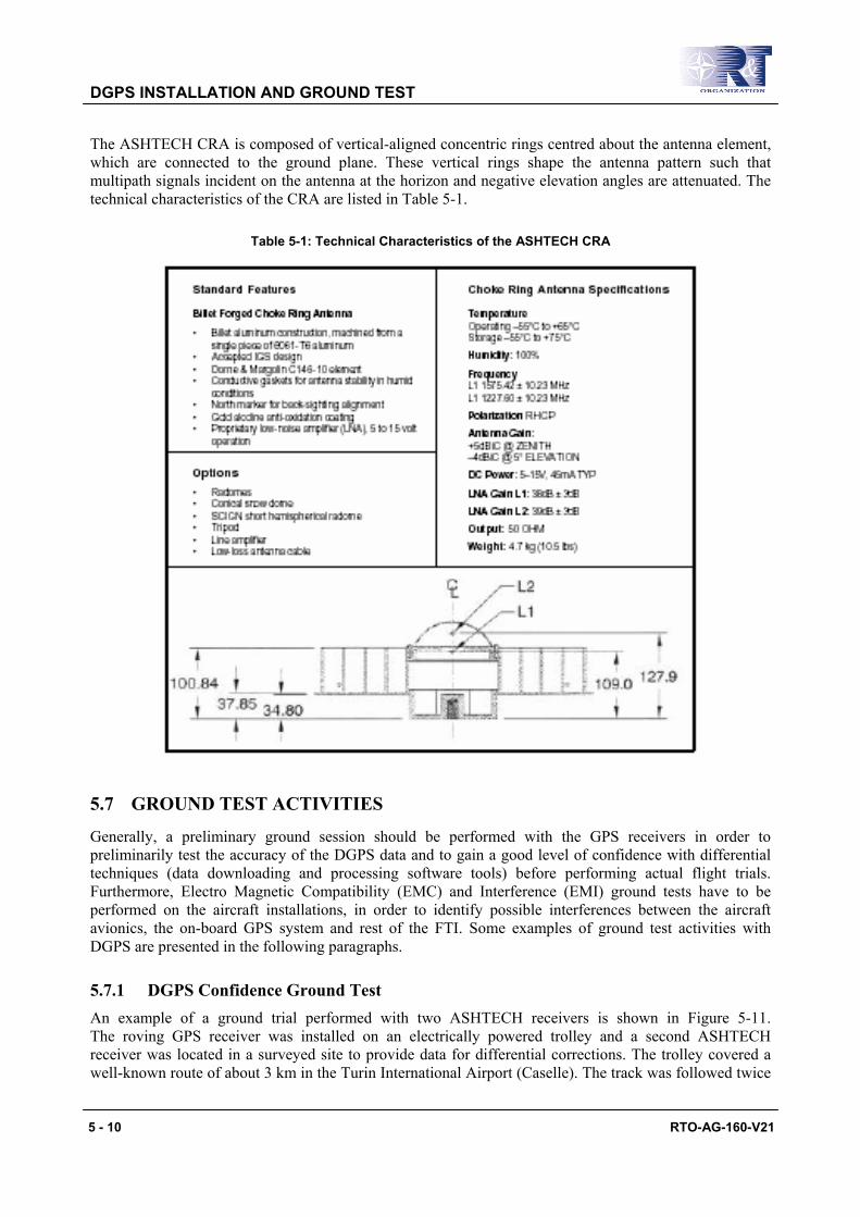
DGPS INSTALLATION AND GROUND TEST

5 - 10 RTO-AG-160-V21

The ASHTECH CRA is composed of vertical-aligned concentric rings centred about the antenna element, which are connected to the ground plane. These vertical rings shape the antenna pattern such that multipath signals incident on the antenna at the horizon and negative elevation angles are attenuated. The technical characteristics of the CRA are listed in Table 5-1.

Table 5-1: Technical Characteristics of the ASHTECH CRA

5.7 GROUND TEST ACTIVITIES

Generally, a preliminary ground session should be performed with the GPS receivers in order to preliminarily test the accuracy of the DGPS data and to gain a good level of confidence with differential techniques (data downloading and processing software tools) before performing actual flight trials. Furthermore, Electro Magnetic Compatibility (EMC) and Interference (EMI) ground tests have to be performed on the aircraft installations, in order to identify possible interferences between the aircraft avionics, the on-board GPS system and rest of the FTI. Some examples of ground test activities with DGPS are presented in the following paragraphs.

5.7.1 DGPS Confidence Ground Test An example of a ground trial performed with two ASHTECH receivers is shown in Figure 5-11. The roving GPS receiver was installed on an electrically powered trolley and a second ASHTECH receiver was located in a surveyed site to provide data for differential corrections. The trolley covered a well-known route of about 3 km in the Turin International Airport (Caselle). The track was followed twice

DGPS INSTALLATION AND GROUND TEST

RTO-AG-160-V21 5 - 11

(in opposite directions) along a road about 6.2 metres wide. After the trial, data stored into the internal memories of the two receivers were downloaded to a personal computer for differential processing and analysed as described in paragraph 5.4. Positioning data after differential processing (pseudorange) and post-processing noise reduction were very accurate. The stand-alone accuracy of the receiver was 22.4 m SEP (SA off) and well within the specifications. The results obtained with C/A code differential processing were also very encouraging with a position data accuracy of 3.1 m SEP.

Figure 5-11: Aerodrome Chart with Reference Station and Trolley Track.

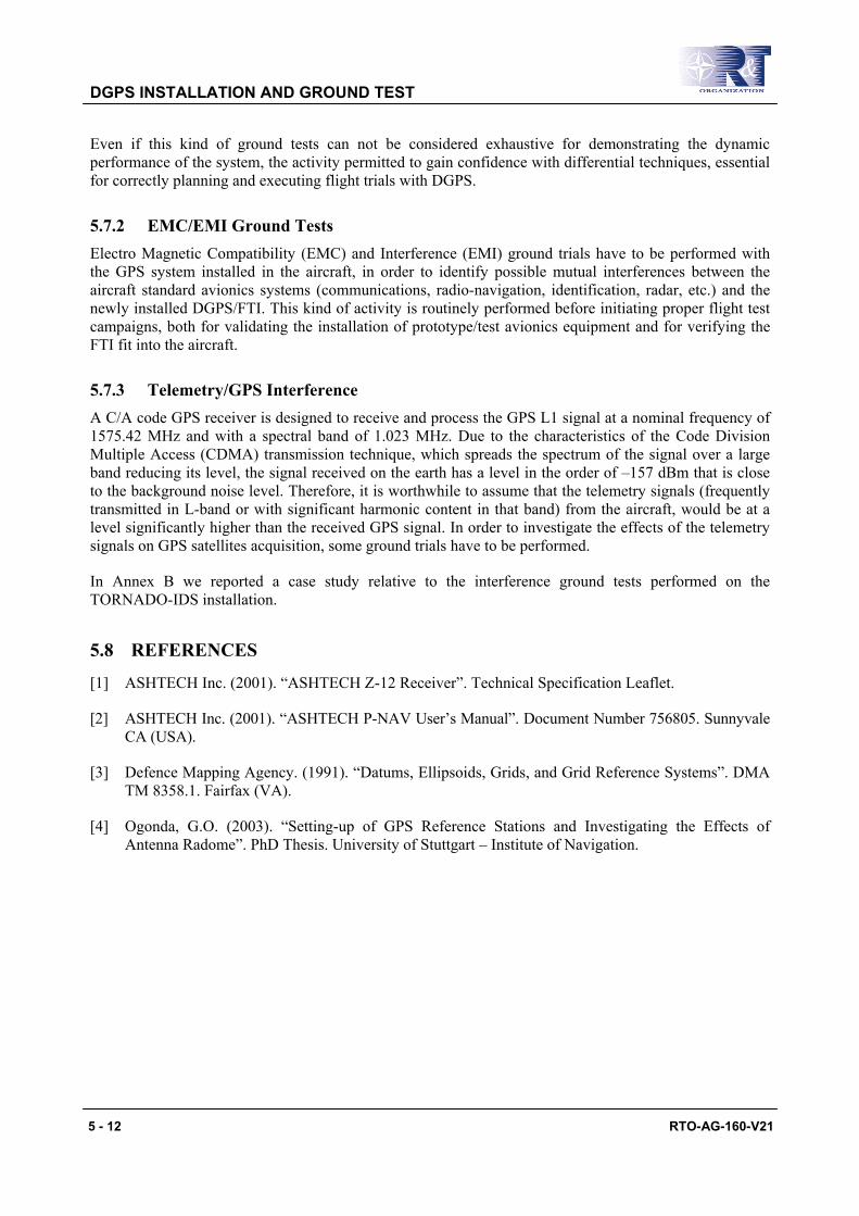
DGPS INSTALLATION AND GROUND TEST

5 - 12 RTO-AG-160-V21

Even if this kind of ground tests can not be considered exhaustive for demonstrating the dynamic performance of the system, the activity permitted to gain confidence with differential techniques, essential for correctly planning and executing flight trials with DGPS.

5.7.2 EMC/EMI Ground Tests Electro Magnetic Compatibility (EMC) and Interference (EMI) ground trials have to be performed with the GPS system installed in the aircraft, in order to identify possible mutual interferences between the aircraft standard avionics systems (communications, radio-navigation, identification, radar, etc.) and the newly installed DGPS/FTI. This kind of activity is routinely performed before initiating proper flight test campaigns, both for validating the installation of prototype/test avionics equipment and for verifying the FTI fit into the aircraft.

5.7.3 Telemetry/GPS Interference A C/A code GPS receiver is designed to receive and process the GPS L1 signal at a nominal frequency of 1575.42 MHz and with a spectral band of 1.023 MHz. Due to the characteristics of the Code Division Multiple Access (CDMA) transmission technique, which spreads the spectrum of the signal over a large band reducing its level, the signal received on the earth has a level in the order of –157 dBm that is close to the background noise level. Therefore, it is worthwhile to assume that the telemetry signals (frequently transmitted in L-band or with significant harmonic content in that band) from the aircraft, would be at a level significantly higher than the received GPS signal. In order to investigate the effects of the telemetry signals on GPS satellites acquisition, some ground trials have to be performed.

In Annex B we reported a case study relative to the interference ground tests performed on the TORNADO-IDS installation.

5.8 REFERENCES

[1] ASHTECH Inc. (2001). “ASHTECH Z-12 Receiver”. Technical Specification Leaflet.

[2] ASHTECH Inc. (2001). “ASHTECH P-NAV User’s Manual”. Document Number 756805. Sunnyvale CA (USA).

[3] Defence Mapping Agency. (1991). “Datums, Ellipsoids, Grids, and Grid Reference Systems”. DMA TM 8358.1. Fairfax (VA).

[4] Ogonda, G.O. (2003). “Setting-up of GPS Reference Stations and Investigating the Effects of Antenna Radome”. PhD Thesis. University of Stuttgart – Institute of Navigation.

RTO-AG-160-V21 6 - 1

Chapter 6 – DGPS PERFORMANCE ANALYSIS

6.1 INTRODUCTION

During flight test activities performed with DGPS, data was analysed with the aim of assessing the performance of the system in flight. A preliminary assessment was carried out on the MB339-CD aircraft. In this phase, only a qualitative evaluation was made in order to verify the performance of both the ASHTECH and the TRIMBLE GPS receivers during high dynamic manoeuvres (mainly in terms of data quality and continuity). Once the dynamic performance of the systems was verified, one of them was selected (i.e., ASHTECH Z-12) and used for the final in-flight evaluation carried out mainly on the TORNADO-IDS aircraft. During these activities the in-flight manoeuvring limitations of the system were investigated and additional instrumentation/analysis was used in order to determine the accuracy provided by the ASHTECH system in flight.

6.2 MB-339CD DGPS IN-FLIGHT INVESTIGATIONS

During the MB-339CD avionics flight trials, performed by AERMACCHI S.p.A. and the Italian Air Force Flight Test Centre, an in-flight evaluation of DGPS was carried out. The aim of this assessment was to compare the performance of the TANS and the ASHTECH receivers (both installed in the prototype aircraft) in a dynamic environment, in order to select the system with the best performance for employment in future activities. Particularly, the assessment focused on the data quality and continuity provided by the two GPS receivers during execution of low, medium, and high dynamics manoeuvres and re-acquisition times after GPS data losses. Therefore, no dedicated accuracy tests were performed in this phase, except an initial evaluation of DGPS altitude data. The results of the MB-339CD in-flight investigation are reported in Annex C.

6.3 TORNADO-IDS DGPS IN-FLIGHT INVESTIGATIONS

Analysing several data from the MB-339CD DGPS test campaign and other flight test activities performed with DGPS instrumented aircraft (i.e., F104 ASA-M, AM-X, EF-2000, MB-339A, TORNADO-IDS, etc.), it was clear that the main disadvantage of the GPS is its vulnerability to signal losses caused by satellites masking and low SNR. Therefore, during some TORNADO-IDS flight trials these problems were thoroughly investigated, to test the capability of the on-board GPS receiver to reacquire satellite signals and to provide TSPI even with degraded satellite constellations. In order to assist in the investigation a simulation tool was used to evaluate the global masking effect due to antenna and aircraft body masking. A preliminary assessment was also carried out of Doppler effects influence on data quality. Moreover, appropriate procedures were defined for the optimal use of DGPS (continuous positioning data gathering with reduced satellite signal losses) in flight test activities with high performance aircraft. Finally, an assessment of DGPS data accuracy was carried out, by comparing the positioning data provided by DGPS with other known references (i.e., radar altimeter, laser range finder and optical tracking system).

6.3.1 Masking and SNR Investigation The main reasons of interruption of the satellite signals in flight tests activities with DGPS are the shielding of the GPS antenna by the aircraft body (especially the wings and the tails) during turns, and the reduction of Signal-to-Noise Ratios (SNR) during high dynamics manoeuvres. In order to investigate GPS antenna masking and the effects of SNR reduction, a dedicated analysis as carried out on TORNADO-IDS. The detailed results of the investigation are reported in Annex D.

DGPS PERFORMANCE ANALYSIS

6 - 2 RTO-AG-160-V21

6.3.2 Flight Test Mission Planning and Optimisation As a result of the Masking/SNR analysis some recommendations were formulated in order to optimise the use of DGPS as a datum in flight test missions (i.e., in order to reduce signal loses). In particular, the following criteria’s should be taken into account:

• It should be always assured the visibility of at least four satellites with an elevation near 50°;

• The maximum bank angle allowed is 50°;

• A stabilisation of at least 20 seconds should precede and follow the significant flight phases;

• The heading variations should be as gradual as possible;

• It should be minimised the number of left turns performed with an initial heading ranging from 45° to 135°, and the number of right turns performed with an initial heading between 225° and 315°; and

• The distance between the aircraft and the ground receiver should be always less than 200 NM.

These restrictions, of course, imply operational limitations that reduce the spread of possible DGPS applications in the flight test environment. Further details are given in Annex D.

6.3.3 Doppler Effect During the initial phase of GPS evaluation it was noted that the reacquisition time after loss of one or more satellites signals could be up to 40 seconds, depending on flight conditions and satellite constellations. We wondered whether and how the Doppler effect could affect the receiver capability to track the carrier phase and rapidly reacquire the signal after a loss.

The typical equation used to express the Doppler shift associated to a certain instantaneous velocity along the line of propagation of the signal, is the following:

fcvf ⋅=∆ (6.1)

where:

∆f = frequency shift;

v = velocity of the receiver;

c = speed of light ( )3 108 1⋅ ⋅ −m s ; and

f = transmitted frequency (in our case 1575.42 MHz).

The Doppler shift directly affects the signal acquisition time of the receiver, both in terms of frequency of the code and frequency of the carrier. In general, the acquisition time increases in presence of Doppler shift as shown in Figure 6-1.

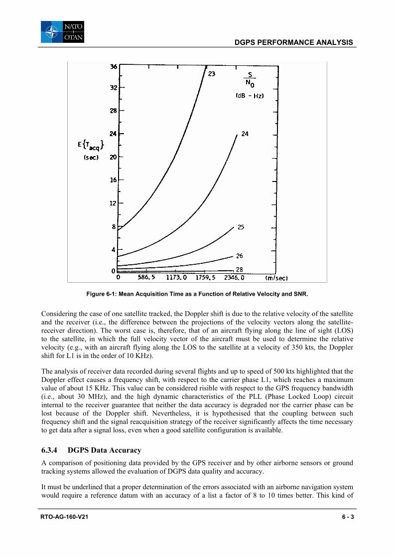
DGPS PERFORMANCE ANALYSIS

RTO-AG-160-V21 6 - 3

Figure 6-1: Mean Acquisition Time as a Function of Relative Velocity and SNR.

Considering the case of one satellite tracked, the Doppler shift is due to the relative velocity of the satellite and the receiver (i.e., the difference between the projections of the velocity vectors along the satellite-receiver direction). The worst case is, therefore, that of an aircraft flying along the line of sight (LOS) to the satellite, in which the full velocity vector of the aircraft must be used to determine the relative velocity (e.g., with an aircraft flying along the LOS to the satellite at a velocity of 350 kts, the Doppler shift for L1 is in the order of 10 KHz).

The analysis of receiver data recorded during several flights and up to speed of 500 kts highlighted that the Doppler effect causes a frequency shift, with respect to the carrier phase L1, which reaches a maximum value of about 15 KHz. This value can be considered risible with respect to the GPS frequency bandwidth (i.e., about 30 MHz), and the high dynamic characteristics of the PLL (Phase Locked Loop) circuit internal to the receiver guarantee that neither the data accuracy is degraded nor the carrier phase can be lost because of the Doppler shift. Nevertheless, it is hypothesised that the coupling between such frequency shift and the signal reacquisition strategy of the receiver significantly affects the time necessary to get data after a signal loss, even when a good satellite configuration is available.

6.3.4 DGPS Data Accuracy A comparison of positioning data provided by the GPS receiver and by other airborne sensors or ground tracking systems allowed the evaluation of DGPS data quality and accuracy.

It must be underlined that a proper determination of the errors associated with an airborne navigation system would require a reference datum with an accuracy of a list a factor of 8 to 10 times better. This kind of

DGPS PERFORMANCE ANALYSIS

6 - 4 RTO-AG-160-V21

reference is obviously very difficult (if not impossible) to be identified in the case of DGPS accuracy testing. The best options available is to use high-accuracy cinetheodolites or laser tracking systems of proven pointing stability, whose quoted accuracy are typically in the order of 0.2 ÷ 0.5 metres. For the TORNADO-IDS DGPS accuracy flight trials, the following position reference systems were used:

• The TORNADO-IDS aircraft Radar Altimeter (R/A);

• Laser range from the Convertible Laser Designation Pod (CLDP) installed on the aircraft; and

• Ground-based optical systems (cinetheodolites).

6.3.4.1 DGPS-Radar Altimeter

A comparison was made between the DGPS-TSPI altitude data and the measurements provided by the on-board radar altimeter, in order to preliminarily assess the DGPS data quality. For this purpose a number of over-sea flight legs were included in the trials.

The ASHTECH DGPS altitude data output was both in the form of geodetic altitude or ellipsoidal height. The height above terrain measured by a Radar Altimeter (R/A) is obviously different from the geodetic height provided by the GPS. Moreover, there is not a fixed relationship between the height above Mean Sea Level (MSL) and the geodetic height. This is due to irregularities of the Geoid (i.e., the equipotential surface defined in the Earth’s gravity field which can be approximated, for some practical applications, to MSL).

Flying over the sea, the R/A height approximated the MSL altitude. As the Geoid-MSL separation was unknown, a certain degree of uniformity was obtained flying round tracks over limited sea areas (i.e., there was an unknown bias in the comparison).

Various tests were carried out with different satellite numbers and PDOP ranging from 2.4 to 5. The differences between DGPS and R/A altitudes were measured in the range 3 ÷ 13 metres. Figure 6-2 shows the GPS and R/A data recorded in one of the flights.

DGPS and R/A Altitude

280

300

320

340

360

380

0 35 70 105 140 175 210 245 280 315 350 385 420 455 490 525 560 595 630 665 700 735 770

Time

AG

L A

ltitu

de (f

t)

Radar Altimeter

DGPS

Poli. (Radar Altimeter)

Figure 6-2: Comparison between DGPS and R/A Data.

DGPS PERFORMANCE ANALYSIS

RTO-AG-160-V21 6 - 5

The R/A data 6th order polynomial fit, shown in the graph, follows quite well the DGPS data trend. The estimated measurement bias was in the order of 7.5 metres. Considering the R/A quoted error of ± 3% (of the height displayed), the results of this preliminary and purely qualitative comparison of DGPS and R/A data were considered satisfactory.

6.3.4.2 DGPS-Laser Range

This evaluation was performed during the TORNADO-IDS flight test activities for integration of the Thomson CLDP (Convertible Laser Designation Pod). These activities were conducted at the Cazaux test range (France).

The CLDP system is designed to provide the aircraft with day and night laser designation/ranging capability, for both cooperative and self-designation attacks performed using laser-guided weapons. The pod is equipped with an internal designation laser operating at 1.064 µm (non-eyesafe region of the spectrum) and may be configured for day-time operation by using a television camera (TV) or for day/ night operation by using an IR sensor (IR). The TV configuration may also provide daytime advantages in high humidity conditions. In its subsidiary role, the CLDP can also act as a sensor for navigation fixing including altitude fixing.

As shown in Figure 6-3, both CLDP configurations consist primarily of two sections: an interchangeable front section containing a TV sensor head or IR sensor head, and a common body containing a central section and a rear cooling unit.

Figure 6-3: CLDP TV and IR Configurations.

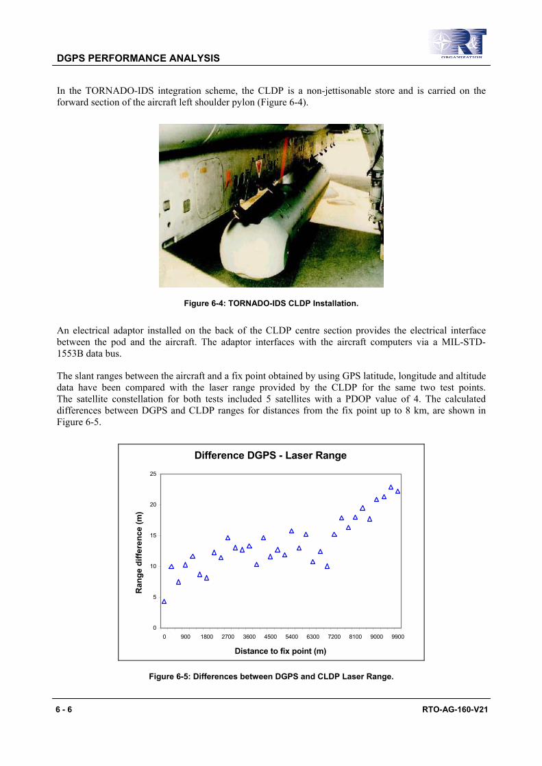
DGPS PERFORMANCE ANALYSIS

6 - 6 RTO-AG-160-V21

In the TORNADO-IDS integration scheme, the CLDP is a non-jettisonable store and is carried on the forward section of the aircraft left shoulder pylon (Figure 6-4).

Figure 6-4: TORNADO-IDS CLDP Installation.

An electrical adaptor installed on the back of the CLDP centre section provides the electrical interface between the pod and the aircraft. The adaptor interfaces with the aircraft computers via a MIL-STD-1553B data bus.

The slant ranges between the aircraft and a fix point obtained by using GPS latitude, longitude and altitude data have been compared with the laser range provided by the CLDP for the same two test points. The satellite constellation for both tests included 5 satellites with a PDOP value of 4. The calculated differences between DGPS and CLDP ranges for distances from the fix point up to 8 km, are shown in Figure 6-5.

Difference DGPS - Laser Range

0

5

10

15

20

25

0 900 1800 2700 3600 4500 5400 6300 7200 8100 9000 9900

Distance to fix point (m)

Ran

ge d

iffer

ence

(m)

Figure 6-5: Differences between DGPS and CLDP Laser Range.

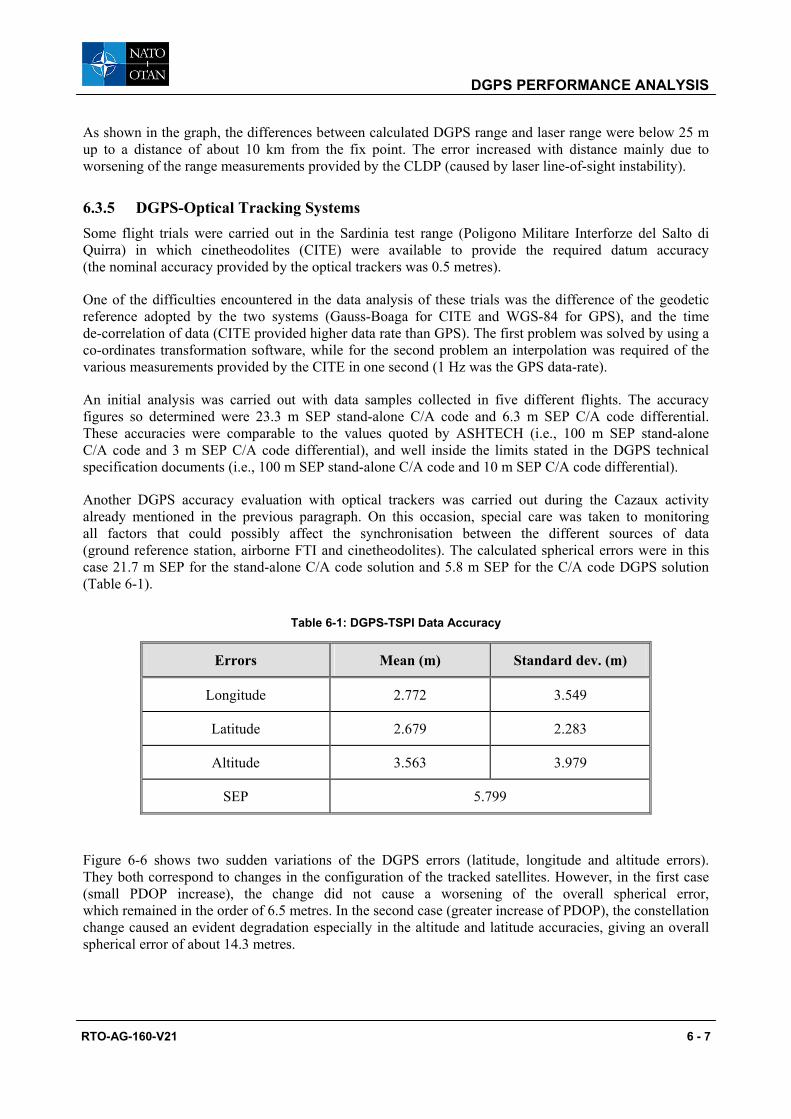
DGPS PERFORMANCE ANALYSIS

RTO-AG-160-V21 6 - 7

As shown in the graph, the differences between calculated DGPS range and laser range were below 25 m up to a distance of about 10 km from the fix point. The error increased with distance mainly due to worsening of the range measurements provided by the CLDP (caused by laser line-of-sight instability).

6.3.5 DGPS-Optical Tracking Systems Some flight trials were carried out in the Sardinia test range (Poligono Militare Interforze del Salto di Quirra) in which cinetheodolites (CITE) were available to provide the required datum accuracy (the nominal accuracy provided by the optical trackers was 0.5 metres).

One of the difficulties encountered in the data analysis of these trials was the difference of the geodetic reference adopted by the two systems (Gauss-Boaga for CITE and WGS-84 for GPS), and the time de-correlation of data (CITE provided higher data rate than GPS). The first problem was solved by using a co-ordinates transformation software, while for the second problem an interpolation was required of the various measurements provided by the CITE in one second (1 Hz was the GPS data-rate).

An initial analysis was carried out with data samples collected in five different flights. The accuracy figures so determined were 23.3 m SEP stand-alone C/A code and 6.3 m SEP C/A code differential. These accuracies were comparable to the values quoted by ASHTECH (i.e., 100 m SEP stand-alone C/A code and 3 m SEP C/A code differential), and well inside the limits stated in the DGPS technical specification documents (i.e., 100 m SEP stand-alone C/A code and 10 m SEP C/A code differential).

Another DGPS accuracy evaluation with optical trackers was carried out during the Cazaux activity already mentioned in the previous paragraph. On this occasion, special care was taken to monitoring all factors that could possibly affect the synchronisation between the different sources of data (ground reference station, airborne FTI and cinetheodolites). The calculated spherical errors were in this case 21.7 m SEP for the stand-alone C/A code solution and 5.8 m SEP for the C/A code DGPS solution (Table 6-1).

Table 6-1: DGPS-TSPI Data Accuracy

Errors Mean (m) Standard dev. (m)

Longitude 2.772 3.549

Latitude 2.679 2.283

Altitude 3.563 3.979

SEP 5.799

Figure 6-6 shows two sudden variations of the DGPS errors (latitude, longitude and altitude errors). They both correspond to changes in the configuration of the tracked satellites. However, in the first case (small PDOP increase), the change did not cause a worsening of the overall spherical error, which remained in the order of 6.5 metres. In the second case (greater increase of PDOP), the constellation change caused an evident degradation especially in the altitude and latitude accuracies, giving an overall spherical error of about 14.3 metres.

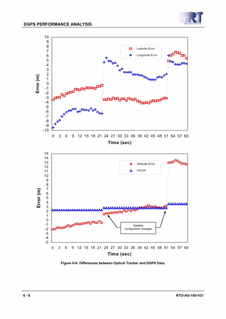
DGPS PERFORMANCE ANALYSIS

6 - 8 RTO-AG-160-V21

-10-9-8-7-6-5-4-3-2-10123456789

10

0 3 6 9 12 15 18 21 24 27 30 33 36 39 42 45 48 51 54 57 60

Time (sec)

Erro

r (m

)

Latitude Error

Longitude Error

-5-4-3-2-10123456789

101112131415

0 3 6 9 12 15 18 21 24 27 30 33 36 39 42 45 48 51 54 57 60

Time (sec)

Erro

r (m

)

Altitude Error

PDOP

Satellite configuration changes

Figure 6-6: Differences between Optical Tracker and DGPS Data.

RTO-AG-160-V21 7 - 1

Chapter 7 – SOME FURTHER APPLICATIONS AND DEVELOPMENTS

7.1 GENERAL

The present chapter focuses on further developments in the field of DGPS for flight testing, including perspectives for future research activities. Particularly, after discussing a simple method for post-processing recover of DGPS data losses, the most important DGPS/INS integration issues are presented, together with typical integrated systems architectures. Moreover, the design features of an optimal DGPS/ INS Position Reference System (PRS) suitable for flight test applications are presented, together with a new approach to the problem of DGPS integrity augmentation, showing potentials for high precision aircraft applications.

7.2 INTEGRATION OF DGPS AND INS MEASUREMENTS

Although many tasks are fulfilled now by sole means of Differential GPS, there are still areas where integration with an INS is necessary. Particularly, in flight testing of modern navigation systems DGPS cannot provide the necessary information with regard to data rate and data continuity during high dynamic manoeuvres. Many studies have been undertaken in order to investigate the potential of DGPS/INS integration for flight test and other high precision applications. Together with real-time C/A code DGPS, also DGPS using carrier phase ambiguity resolution on-the-fly has been investigated and different options for the INS mechanisation have been considered. The integrated PRS is being conceived primarily for testing of modern navigation and landing systems (e.g., satellite systems and integrated systems); however, due to the high accuracy and data rates obtainable with DGPS/INS integration, the system will also be suitable for other tasks, such as aircraft noise certification, and most of current avionics and armament experimental tasks.

In the following paragraphs only the main results achieved are presented. The fundamentals of DGPS/INS integration are presented in Annex E.

7.2.1 Recovering DGPS Data Losses A simple method has been developed for post-processing recover of DGPS data losses due to antenna masking, hard manoeuvring or bad satellite configuration. The method utilises the direct integration of data provided by the on-board INS starting from an initial reliable position determined by DGPS (i.e., obtained after a stabilisation of at least 20 seconds, with at least 4 satellites in view and PDOP<3). The integration is carried out up to the next reliable DGPS relief. The difference at the end of integration between the so calculated aircraft position and that provided by DGPS enables the determination of the average value of the inertial drift derivative with respect to time, which is used to minimise the inertial error during reconstruction of the aircraft trajectory for the whole time slice considered. So, it is possible to provide an accurate aircraft trajectory even when the manoeuvres can lead to GPS data losses, without the use of external reference systems (e.g., cinetheodolites, tracking radars) or pilot fixes, which require good weather conditions and properly instrumented test ranges.

In Figure 7-1(a), referring to three consecutive orbits lasting for about eleven minutes, DGPS latitude data are compared with inertial latitude corrected by using the method described above. The difference between the two sets of data (i.e., DGPS/INS latitude error) is magnified in Figure 7-1(b) and compared with the inertial latitude error without DGPS corrections.

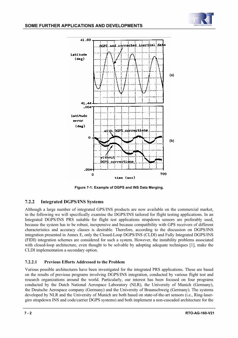
SOME FURTHER APPLICATIONS AND DEVELOPMENTS

7 - 2 RTO-AG-160-V21

Figure 7-1: Example of DGPS and INS Data Merging.

7.2.2 Integrated DGPS/INS Systems Although a large number of integrated GPS/INS products are now available on the commercial market, in the following we will specifically examine the DGPS/INS tailored for flight testing applications. In an Integrated DGPS/INS PRS suitable for flight test applications strapdown sensors are preferably used, because the system has to be robust, inexpensive and because compatibility with GPS receivers of different characteristics and accuracy classes is desirable. Therefore, according to the discussion on DGPS/INS integration presented in Annex E, only the Closed-Loop DGPS/INS (CLDI) and Fully Integrated DGPS/INS (FIDI) integration schemes are considered for such a system. However, the instability problems associated with closed-loop architecture, even thought to be solvable by adopting adequate techniques [1], make the CLDI implementation a secondary option.

7.2.2.1 Previous Efforts Addressed to the Problem

Various possible architectures have been investigated for the integrated PRS applications. These are based on the results of previous programs involving DGPS/INS integration, conducted by various flight test and research organizations around the world. Particularly, our interest has been focused on four programs conducted by the Dutch National Aerospace Laboratory (NLR), the University of Munich (Germany), the Deutsche Aerospace company (Germany) and the University of Braunschweig (Germany). The systems developed by NLR and the University of Munich are both based on state-of-the-art sensors (i.e., Ring-laser-giro strapdown INS and code/carrier DGPS systems) and both implement a non-cascaded architecture for the

(a)

(b)

SOME FURTHER APPLICATIONS AND DEVELOPMENTS

RTO-AG-160-V21 7 - 3

Kalman filter. Particularly, NLR developed a PRS for testing the Fokker 70 aircraft, and the University of Munich (IAPG) designed a high-precision aircraft navigation/landing system based on DGPS/INS integration. The results of the NLR DGPS/INS development program have been published by Van de Leijgraaf [2] and Kannemans [3]. The results of the research conducted at the University of Munich (IAPG) have been described by Hein [4]. The DGPS/INS integrated landing system developed by Deutsche Aerospace has been described by Jacob [5], and the integrated precision navigation system (DGPS/INS) developed by the University of Braunschweig has been described by Shanzer [6].

The most interesting system architectures, from our point of view, are those of the NLR and IAPG systems, both adopting a fully integrated approach. The main difference between the two systems is that they use different DGPS information as input to the Kalman filter. This makes the structure of the various software modules (including the Kalman filter itself) quite different in the two cases. While both systems use similar INS inputs (i.e., RLG and accelerometer raw data), in the first case GPS position (and velocity) data are delivered (de-correlated between update intervals using an ad-hoc algorithm) by a differential processing module (which processes data from both the ground and the airborne receivers), while the system proposed by IAPG uses the raw (uncorrelated) DGPS data (i.e., differentially corrected pseudoranges, carrier phases, range rates) as direct input to the Kalman filter. Both approaches have significant advantages and drawbacks. Therefore, a closer look at the NLR and IAPG systems is important.

7.2.2.2 NLR System

Since the NLR system has been conceived to use either standalone GPS (C/A code), differential code range GPS (C/A code) or differential carrier range GPS (L1 and L2) depending on the required accuracy (i.e., 100 metres, 5 metres, and 0.15 metres respectively), the computer software modules have been designed to accomplish with this requirement. Particularly, the system includes:

• A module for processing C/A code pseudoranges from both the airborne and ground receivers (DCA module);

• A module for processing L1 and L2 carrier ranges from both the airborne and ground receivers (DCR module);

• A module for integration of DGPS and INS measurements (IDI module); and

• A module for comparing the computed positions with a pre-defined aircraft trajectory and sending guidance information to a cockpit display.

In the NLR system, when DGPS data is absent for short time intervals, the calibrated INS maintains the required accuracy. The length of the allowable interruption depends on the required accuracy and the accuracy of the estimated INS errors just before the interruption. The Kalman filter uses an INS error model, raw INS data and DGPS position and velocity data, which are uncorrelated between update intervals.

From the covariance matrix of a full DGPS solution (provided either by the DCA or the DCR module), the position (and velocity) dependent part can be derived (i.e., three dimensional measurement vectors). In fact, the computations of the DCA and DCR modules are performed so that the square root information matrices of the position and velocity solutions are made available for the IDI module. Clearly, the components of an estimated position vector are mutually correlated and so are the components of an estimated velocity vector. By multiplying the difference between the calculated position (and velocity) vector and the raw INS position (and velocity) vector by its associated square root information matrix, a transformed measurement vector with uncorrelated components is obtained. This vector (and its velocity counterpart) are then processed component-wise by the Kalman filter. As the noise on the carrier ranges is much smaller than the noise on the code ranges, the standard deviations of INS error estimates are correspondingly smaller [3].

SOME FURTHER APPLICATIONS AND DEVELOPMENTS

7 - 4 RTO-AG-160-V21

7.2.2.3 IAPG System

The IAPG system has been designed for using, in real-time, DGPS carrier phase corrections transmitted from the ground Reference Station. Therefore, the system can provide only a high precision DGPS/INS solution (carrier phase positioning about 5 centimetres accuracy). In contrary to the NLR system, there is no provision for a low accuracy (C/A code, 100 metres) or a medium accuracy service (i.e., differential code-range, about 5 metres) to be provided in real-time. The Kalman filter has been designed to accept INS raw data and GPS raw data (i.e., pseudoranges, carrier phases, range rates) corrected with data transmitted from the ground (i.e., pseudorange and carrier phase corrections), in order to provide the high accuracy integrated solution.

The use of GPS carrier phase observation requires that the initial ambiguities have to be determined. It is therefore necessary, for real-time operation, that this starting procedure is performed during the aircraft flight (i.e., OTF ambiguity resolution) as well as after periods of signal loss-of-lock. If cycle slips occur (without a longer period of loss- of-lock) during the operation, the Kalman filter is able to solve for it due to the INS observations. However, there is a time limit for a complete GPS outage in the range of 20 to 40 seconds. If the loss-of-lock period is longer, a degradation in accuracy has to be accepted before the OTF algorithm can perform the initialisation good to the last cycle.

Also for the INS it has been assumed that, in certain operational conditions, a static initialisation (i.e., initial alignment) cannot be performed on the ground and in-flight alignment methods (with related accuracy degradation) have been considered. Furthermore, coning and sculling effects of the INS have been compensated carefully [4].

7.2.3 An Optimal PRS for Flight Testing An optimal PRS should include solutions from both the NLR and IAPG systems. Particularly, according to flight test requirements, the PRS should be able to cover various accuracy classes:

• A low accuracy class with stand alone GPS (C/A-code, nominal position accuracy 100 m 2D-RMS and less than 50 m practical in the absence of SA) updating the INS. This is required for the evaluation/certification of medium-range navigation sensors and systems (VOR/DME, TACAN, NDB, ADF, etc.); and

• A high accuracy class (3-D position accuracy at the decimetre level), in which differential carrier range measurements can be used to update the INS. This is required for a number of applications, such as aircraft noise certification, evaluation of landing systems and determination of aircraft take-off and landing performance.

A bi-directional data link would be required to transmit the differential corrections from the ground reference station to the aircraft. This would enable real-time position calculation in the aircraft and provide (optionally) guidance information to the pilot. Without the data link the system will automatically degrade to the low accuracy mode (e.g., out-of-range operations).

7.2.3.1 Hardware Set-up

Based on the results of our investigation, the basic hardware set-up shown in Figure 7-2 is considered an ideal solution for flight test applications. The computer receives raw data from the airborne GPS (i.e., pseudoranges, carrier phases, satellite orbit parameters), correction data from the ground GPS receiver at the Reference Station (i.e., pseudoranges and carrier phase corrections), and raw data from the INS.

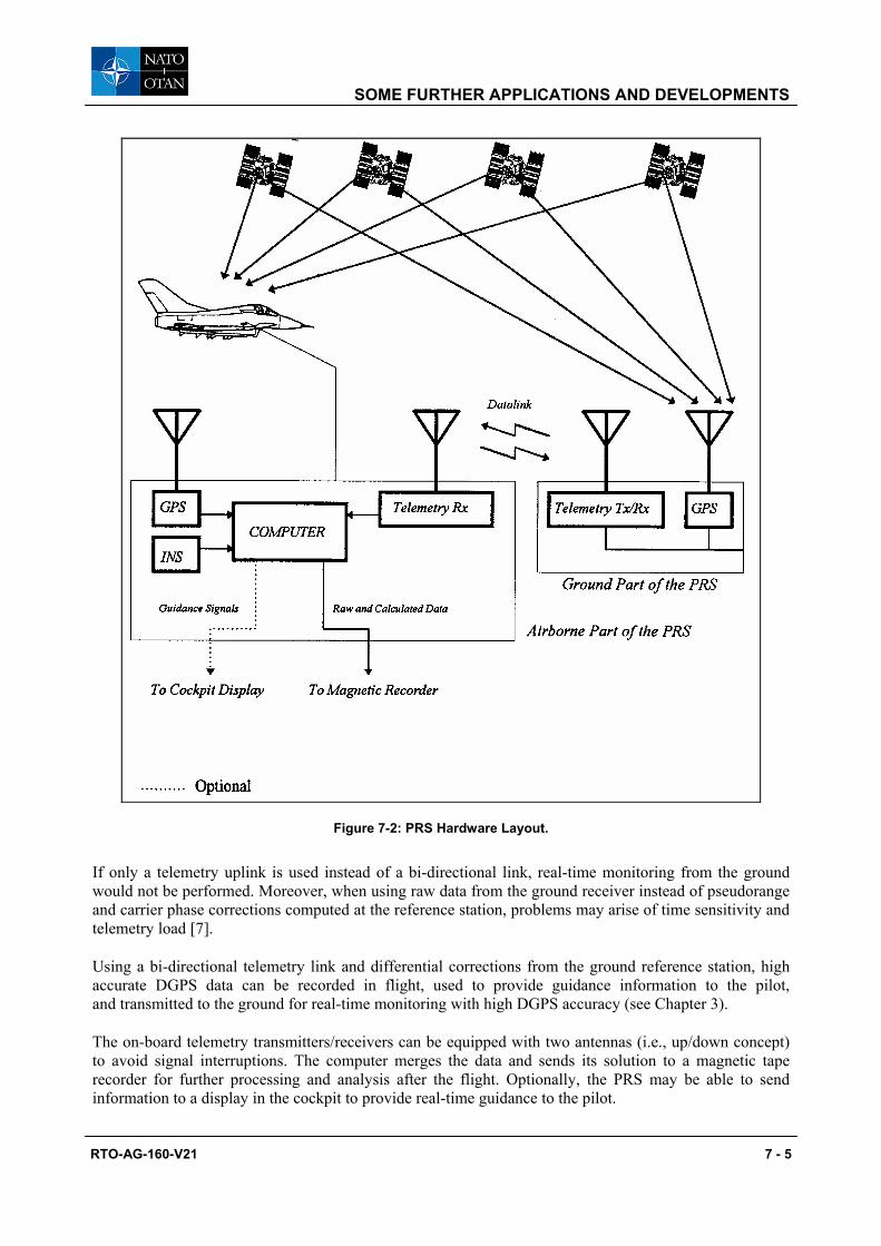
SOME FURTHER APPLICATIONS AND DEVELOPMENTS

RTO-AG-160-V21 7 - 5

Figure 7-2: PRS Hardware Layout.

If only a telemetry uplink is used instead of a bi-directional link, real-time monitoring from the ground would not be performed. Moreover, when using raw data from the ground receiver instead of pseudorange and carrier phase corrections computed at the reference station, problems may arise of time sensitivity and telemetry load [7].

Using a bi-directional telemetry link and differential corrections from the ground reference station, high accurate DGPS data can be recorded in flight, used to provide guidance information to the pilot, and transmitted to the ground for real-time monitoring with high DGPS accuracy (see Chapter 3).

The on-board telemetry transmitters/receivers can be equipped with two antennas (i.e., up/down concept) to avoid signal interruptions. The computer merges the data and sends its solution to a magnetic tape recorder for further processing and analysis after the flight. Optionally, the PRS may be able to send information to a display in the cockpit to provide real-time guidance to the pilot.

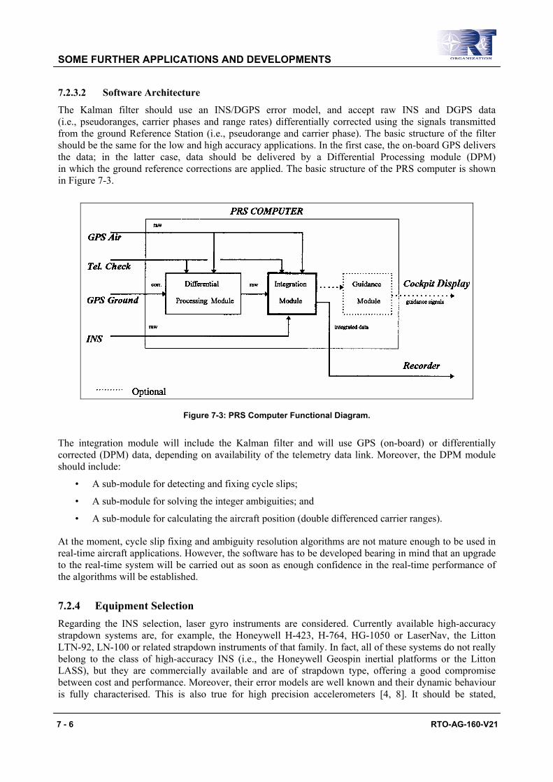
SOME FURTHER APPLICATIONS AND DEVELOPMENTS

7 - 6 RTO-AG-160-V21

7.2.3.2 Software Architecture

The Kalman filter should use an INS/DGPS error model, and accept raw INS and DGPS data (i.e., pseudoranges, carrier phases and range rates) differentially corrected using the signals transmitted from the ground Reference Station (i.e., pseudorange and carrier phase). The basic structure of the filter should be the same for the low and high accuracy applications. In the first case, the on-board GPS delivers the data; in the latter case, data should be delivered by a Differential Processing module (DPM) in which the ground reference corrections are applied. The basic structure of the PRS computer is shown in Figure 7-3.

Figure 7-3: PRS Computer Functional Diagram.

The integration module will include the Kalman filter and will use GPS (on-board) or differentially corrected (DPM) data, depending on availability of the telemetry data link. Moreover, the DPM module should include:

• A sub-module for detecting and fixing cycle slips;

• A sub-module for solving the integer ambiguities; and

• A sub-module for calculating the aircraft position (double differenced carrier ranges).

At the moment, cycle slip fixing and ambiguity resolution algorithms are not mature enough to be used in real-time aircraft applications. However, the software has to be developed bearing in mind that an upgrade to the real-time system will be carried out as soon as enough confidence in the real-time performance of the algorithms will be established.

7.2.4 Equipment Selection Regarding the INS selection, laser gyro instruments are considered. Currently available high-accuracy strapdown systems are, for example, the Honeywell H-423, H-764, HG-1050 or LaserNav, the Litton LTN-92, LN-100 or related strapdown instruments of that family. In fact, all of these systems do not really belong to the class of high-accuracy INS (i.e., the Honeywell Geospin inertial platforms or the Litton LASS), but they are commercially available and are of strapdown type, offering a good compromise between cost and performance. Moreover, their error models are well known and their dynamic behaviour is fully characterised. This is also true for high precision accelerometers [4, 8]. It should be stated,

SOME FURTHER APPLICATIONS AND DEVELOPMENTS

RTO-AG-160-V21 7 - 7

however, that some of these units have aggressive filtering on the data output. For some applications the phase delay associated with these filters may determine lower data rates than required. For high dynamics applications, also the Litton LN200 FOG unit and the Honeywell HG1700 IMU are considered, which can provide data rates of up to 400 and 600 Hz respectively.

Regarding the DGPS component, various dual frequency eight to twelve channels GPS receivers are considered, delivering pseudoranges and carrier phases with full wavelength also in the presence of the P(Y)-code, through cross-correlation or similar techniques. Examples are the TurboRogue SNR-8000 of Allen Osborne Associates Inc., the Trimble 4000-SSE, and the ASHTECH Z-12 and X-treme GPS receivers.

The airborne computer should be based on a state-of-the-art microprocessor and the interface between the systems should be made with an ARINC-429 or MIL-STD-1553-B avionic bus, while communications with the telemetry receiver and the airborne GPS receiver can be guaranteed via RS-232 serial interfaces. The computer boards and the GPS receivers should be designed for airborne use. However, since this can be a serious constraint in the development phase, commercially available equipment can be initially installed in flight qualified housing to protect them by the severe conditions that can be encountered in the aircraft environment (i.e., temperature, vibrations, EMI) and vice versa.

7.2.5 Kalman Filter Design The DGPS/INS Kalman filter may include up to 98-error states [9], but simplifications are possible, and provide acceptable performance with significant state reduction [10]. Covariance analysis is an efficient and powerful tool for sensitivity performance analysis to determine the contributions of distinct error sources. It is essential for developing a robust filter design of minimum state size. Its simulation analysis consists of three major components [2, 11]:

• An aircraft trajectory generator which provides nominal flight data;

• A reference sensor error truth model which characterises all the sensor errors; and

• The reduced-order Kalman filter design to be evaluated.

To conduct sensitivity performance analysis, a covariance analysis is performed with the reduced order Kalman filter, and the gain history is recorded. Then another covariance analysis is performed using the truth model for all sensor errors, with the Kalman filter gain computed from the earlier step. The performance obtained in the second covariance analysis represents the predicted performance of the reduced order filter design [10]. Detailed guidance information for the DGPS/INS Kalman filter design may be found in reference [8, 10, 12, 13].

7.2.6 PRS Testing Once enough confidence has been gained in the performance of the Kalman filter, laboratory testing should be carried out in order to optimise the hardware and software architectures and to give a first estimation of the overall system accuracy. Flight test requirements for a PRS should be similar to the navigation system. test requirements described in Chapter 4. Therefore, in order to prove that a PRS based on GPS/INS integration meets its accuracy requirements, an independent reference system. is needed with an accuracy of at least a factor 3 (preferably 10). Moreover, the verification should be carried out in the environment where the PRS has to operate: on the runway and over the full flight envelope of modern military aircraft. Unfortunately a reference system with the required accuracy in the relevant operational environment is not available. Therefore, the above-described philosophy must be traded in for a practical test philosophy, which would still enable the establishment of the system performance. In fact, a PRS consists of a number of components, each contributing to the total error. The practical test philosophy should be as follows [14]:

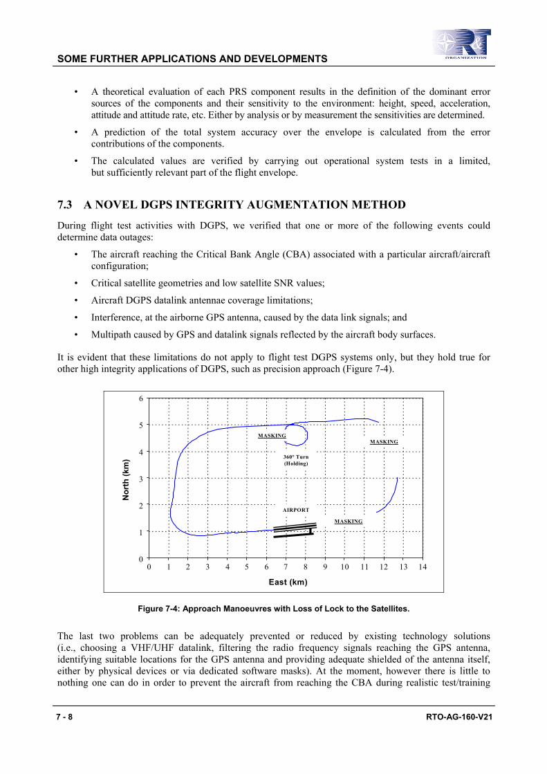
SOME FURTHER APPLICATIONS AND DEVELOPMENTS

7 - 8 RTO-AG-160-V21

• A theoretical evaluation of each PRS component results in the definition of the dominant error sources of the components and their sensitivity to the environment: height, speed, acceleration, attitude and attitude rate, etc. Either by analysis or by measurement the sensitivities are determined.

• A prediction of the total system accuracy over the envelope is calculated from the error contributions of the components.

• The calculated values are verified by carrying out operational system tests in a limited, but sufficiently relevant part of the flight envelope.

7.3 A NOVEL DGPS INTEGRITY AUGMENTATION METHOD

During flight test activities with DGPS, we verified that one or more of the following events could determine data outages:

• The aircraft reaching the Critical Bank Angle (CBA) associated with a particular aircraft/aircraft configuration;

• Critical satellite geometries and low satellite SNR values;

• Aircraft DGPS datalink antennae coverage limitations;

• Interference, at the airborne GPS antenna, caused by the data link signals; and

• Multipath caused by GPS and datalink signals reflected by the aircraft body surfaces.

It is evident that these limitations do not apply to flight test DGPS systems only, but they hold true for other high integrity applications of DGPS, such as precision approach (Figure 7-4).

AIRPORT

360° Turn (Holding)

MASKING

MASKING

MASKING

0

1

2

3

4

5

6

0 1 2 3 4 5 6 7 8 9 10 11 12 13 14

Nor

th (k

m)

East (km)

AIRPORT

360° Turn (Holding)

MASKING

MASKING

MASKING

0

1

2

3

4

5

6

0 1 2 3 4 5 6 7 8 9 10 11 12 13 14

Nor

th (k

m)

East (km)

Figure 7-4: Approach Manoeuvres with Loss of Lock to the Satellites.

The last two problems can be adequately prevented or reduced by existing technology solutions (i.e., choosing a VHF/UHF datalink, filtering the radio frequency signals reaching the GPS antenna, identifying suitable locations for the GPS antenna and providing adequate shielded of the antenna itself, either by physical devices or via dedicated software masks). At the moment, however there is little to nothing one can do in order to prevent the aircraft from reaching the CBA during realistic test/training

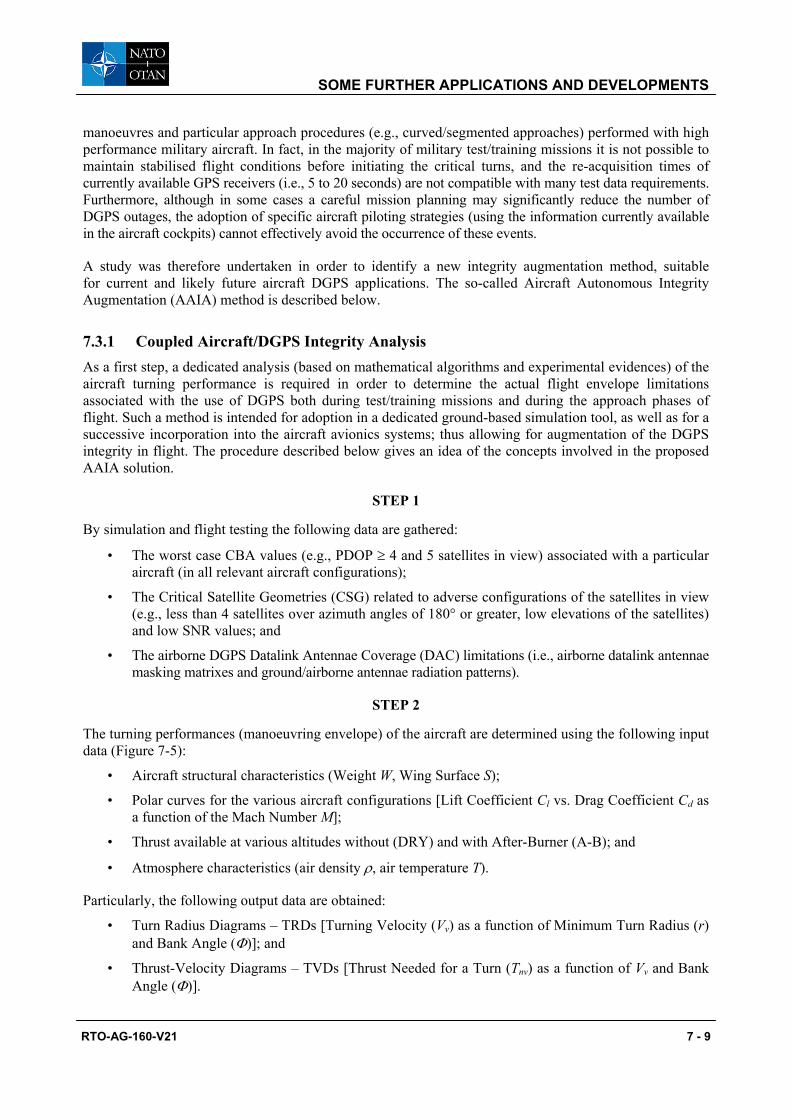
SOME FURTHER APPLICATIONS AND DEVELOPMENTS

RTO-AG-160-V21 7 - 9

manoeuvres and particular approach procedures (e.g., curved/segmented approaches) performed with high performance military aircraft. In fact, in the majority of military test/training missions it is not possible to maintain stabilised flight conditions before initiating the critical turns, and the re-acquisition times of currently available GPS receivers (i.e., 5 to 20 seconds) are not compatible with many test data requirements. Furthermore, although in some cases a careful mission planning may significantly reduce the number of DGPS outages, the adoption of specific aircraft piloting strategies (using the information currently available in the aircraft cockpits) cannot effectively avoid the occurrence of these events.

A study was therefore undertaken in order to identify a new integrity augmentation method, suitable for current and likely future aircraft DGPS applications. The so-called Aircraft Autonomous Integrity Augmentation (AAIA) method is described below.

7.3.1 Coupled Aircraft/DGPS Integrity Analysis As a first step, a dedicated analysis (based on mathematical algorithms and experimental evidences) of the aircraft turning performance is required in order to determine the actual flight envelope limitations associated with the use of DGPS both during test/training missions and during the approach phases of flight. Such a method is intended for adoption in a dedicated ground-based simulation tool, as well as for a successive incorporation into the aircraft avionics systems; thus allowing for augmentation of the DGPS integrity in flight. The procedure described below gives an idea of the concepts involved in the proposed AAIA solution.

STEP 1

By simulation and flight testing the following data are gathered:

• The worst case CBA values (e.g., PDOP ≥ 4 and 5 satellites in view) associated with a particular aircraft (in all relevant aircraft configurations);

• The Critical Satellite Geometries (CSG) related to adverse configurations of the satellites in view (e.g., less than 4 satellites over azimuth angles of 180° or greater, low elevations of the satellites) and low SNR values; and

• The airborne DGPS Datalink Antennae Coverage (DAC) limitations (i.e., airborne datalink antennae masking matrixes and ground/airborne antennae radiation patterns).

STEP 2

The turning performances (manoeuvring envelope) of the aircraft are determined using the following input data (Figure 7-5):

• Aircraft structural characteristics (Weight W, Wing Surface S);

• Polar curves for the various aircraft configurations [Lift Coefficient Cl vs. Drag Coefficient Cd as a function of the Mach Number M];

• Thrust available at various altitudes without (DRY) and with After-Burner (A-B); and

• Atmosphere characteristics (air density ρ, air temperature T).

Particularly, the following output data are obtained:

• Turn Radius Diagrams – TRDs [Turning Velocity (Vv) as a function of Minimum Turn Radius (r) and Bank Angle (Φ)]; and

• Thrust-Velocity Diagrams – TVDs [Thrust Needed for a Turn (Tnv) as a function of Vv and Bank Angle (Φ)].

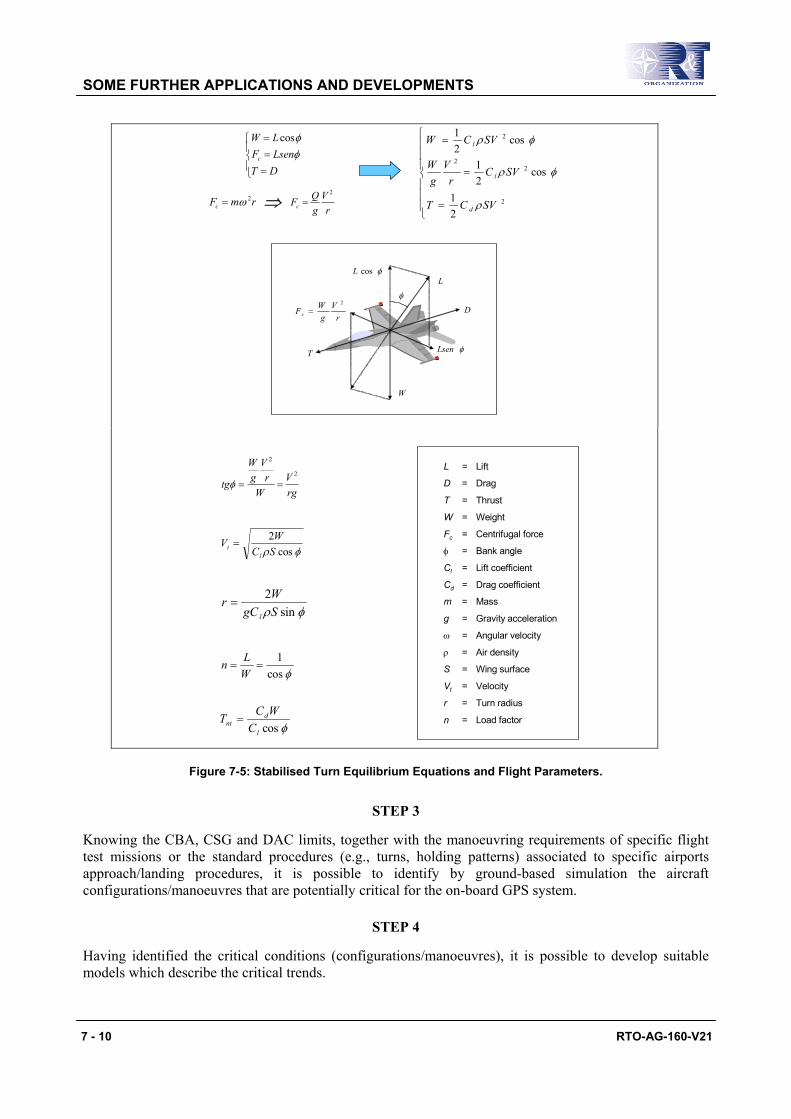
SOME FURTHER APPLICATIONS AND DEVELOPMENTS

7 - 10 RTO-AG-160-V21

===

DTLsenFLW

c φφcos

=

=

=

2

22

2

21

cos21

cos21

SVCT

SVCrV

gW

SVCW

d

l

l

ρ

φρ

φρ

rmFc2ω=

rV

gQFc

2

=⇒

W

rV

gWFc

2

=

L

φ

φcosL

φLsenT

D

rgV

WrV

gW

tg2

2

==φ

φρ cos2SCWV

lt =

φρ sin2SgCWr

l

=

φcos1

==WLn

φcosl

dnt C

WCT =

L = Lift

D = Drag

T = Thrust

W = Weight

Fc = Centrifugal force

φ = Bank angle

Cl = Lift coefficient

Cd = Drag coefficient

m = Mass

g = Gravity acceleration

ω = Angular velocity

ρ = Air density

S = Wing surface

Vt = Velocity

r = Turn radius

n = Load factor

Figure 7-5: Stabilised Turn Equilibrium Equations and Flight Parameters.

STEP 3

Knowing the CBA, CSG and DAC limits, together with the manoeuvring requirements of specific flight test missions or the standard procedures (e.g., turns, holding patterns) associated to specific airports approach/landing procedures, it is possible to identify by ground-based simulation the aircraft configurations/manoeuvres that are potentially critical for the on-board GPS system.

STEP 4

Having identified the critical conditions (configurations/manoeuvres), it is possible to develop suitable models which describe the critical trends.

SOME FURTHER APPLICATIONS AND DEVELOPMENTS

RTO-AG-160-V21 7 - 11

STEP 5

Using these models (e.g., polynomial coefficients, which can be easily incorporated into real-time software look-up tables), and comparing them with the boundaries set by the required Time-to-alarm (TTA) thresholds, it is possible:

• To determine if a specific manoeuvre required for flight test or precision approach can be performed with/without DGPS outages; and

• To generate timely warnings when the aircraft is performing critical manoeuvres prone to induce DGPS outages.

7.3.2 TORNADO-IDS Case Study • A case study was performed in order to determine the potentials of an AAIA system on the

TORNADO-IDS aircraft. For simplicity, only the experimentally determined aircraft CBA limits are considered here. The TORNADO-IDS experimental CBA values (one dorsal antenna) for the various aircraft wing configurations (A, B and C) are given in Figure 7-6.

• CONF. A – 25° ⇒ 42° CBA • CONF. B – 45° ⇒ 47° CBA • CONF. C – 67° ⇒ 55° CBA

67° 25°

Figure 7-6: TORNADO-IDS CBA Values.

After analysis, the following results were obtained:

• Determination of the manoeuvring envelope areas were the CBA can be reached;

• Aircraft turn radius limitations at various altitudes and with various engine power settings; and

• Verification of compatibility between the profiles/procedures required for test and training (e.g., the altitude, velocity), and the CBA limitations.

The main results of the TORNADO-IDS case study are the following:

• The manoeuvring limits are compatible with currently published ILS/MLS approach procedures in the configurations A and B;

• The manoeuvring limits far exceed the DGPS flight test procedures for optimal data gathering (navigation/landing systems flight test applications);

• The CBA can be reached in all aircraft wing configurations (A, B, and C) for altitudes MSL between 0 and 5000 metres;

• The CBA can be reached between 7000 and 10000 metres MSL only with configurations B and C; and

• The CBA can be reached at an altitude of 10000 metres only with the configuration C.

SOME FURTHER APPLICATIONS AND DEVELOPMENTS

7 - 12 RTO-AG-160-V21

An example of the results obtained for the TORNADO-IDS aircraft in configuration C (67° wing sweep) at an altitude of 0 ft MSL (Z = 0) are shown in Figure 7-7, where the envelopes applicable to navigation systems flight test and ILS/MLS precision approach tasks (curved and segmented approaches) are over-imposed to the aircraft TVD and TRD diagrams obtained by analysis.

Figure 7-7: Performance Analysis Results (Examples).

7.3.3 Possible AAIA System Architecture Once the reliability of the mathematical algorithms for AAIA is established, a DGPS integrity augmentation system can be implemented (in the aircraft) for alerting the pilot when the critical conditions for DGPS signal losses are likely to occur (within the specified maximum TTA). The possible architecture of an AAIA system is shown in Figure 7-8.

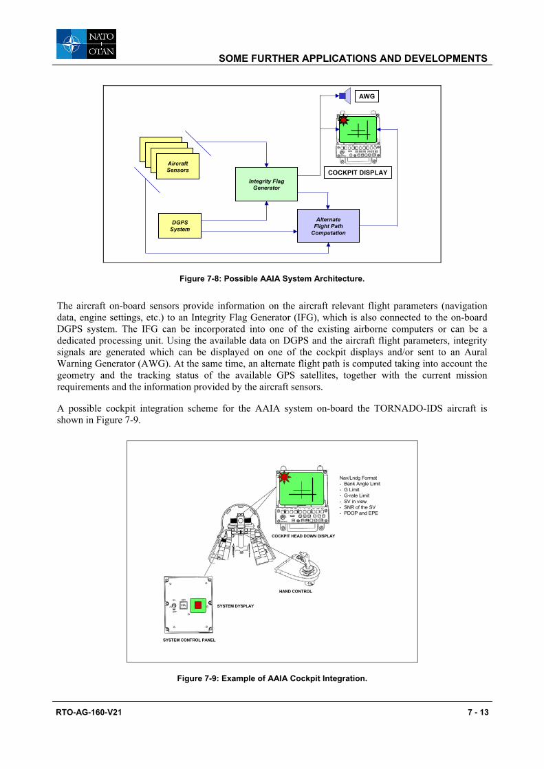
SOME FURTHER APPLICATIONS AND DEVELOPMENTS

RTO-AG-160-V21 7 - 13

HAND CONTROL

SYSTEM CONTROL PANEL

SYSTEM DYSPLAY

AircraftSensors

AlternateFlight Path

Computation

COCKPIT DISPLAYIntegrity Flag

Generator

DGPSSystem

AWG

Figure 7-8: Possible AAIA System Architecture.

The aircraft on-board sensors provide information on the aircraft relevant flight parameters (navigation data, engine settings, etc.) to an Integrity Flag Generator (IFG), which is also connected to the on-board DGPS system. The IFG can be incorporated into one of the existing airborne computers or can be a dedicated processing unit. Using the available data on DGPS and the aircraft flight parameters, integrity signals are generated which can be displayed on one of the cockpit displays and/or sent to an Aural Warning Generator (AWG). At the same time, an alternate flight path is computed taking into account the geometry and the tracking status of the available GPS satellites, together with the current mission requirements and the information provided by the aircraft sensors.

A possible cockpit integration scheme for the AAIA system on-board the TORNADO-IDS aircraft is shown in Figure 7-9.

HAND CONTROL

SYSTEM CONTROL PANEL

COCKPIT HEAD DOWN DISPLAY

SYSTEM DYSPLAY

Nav/Lndg Format- Bank Angle Limit- G Limit- G-rate Limit- SV in view- SNR of the SV- PDOP and EPE

Figure 7-9: Example of AAIA Cockpit Integration.

SOME FURTHER APPLICATIONS AND DEVELOPMENTS

7 - 14 RTO-AG-160-V21

7.4 REFERENCES

[1] Kerr, T.H. (1987). “Decentralized Filtering and Redundancy Management for Multisensor Navigation”. IEEE Transactions on Aerospace and Electronic Systems. AES-23(1).

[2] Van de Leijgraaf, R. (1993). Breeman, J., Moek, G. and Van Leeuwen, S.S., “A Position Reference System for Fokker 70”. NLR Technical Publication TP-93084L.

[3] Kannemans, H. and Van Leeuwen, S.S. (1997). “Development of a Position Reference System for Flight Tests based on GPS”. NLR Technical Publication TP-97483U. Presented at the 9th World Congress of the International Association of Institutes of Navigation”. Amsterdam (The Netherlands).

[4] Hein, G.W. and Ertel, M.M. (1993). “High-precision Aircraft Navigation using DGPS/INS integration”. Institute of Astronomical and Physical Geodesy (IAPG). University FAF Munich, Neubiberg (Germany).

[5] Jacob, T., Meyer, J. and Wacker, U. (1993). “Integrated Navigation and Landing System Using Global Positioning System”. 2nd International Symposium on Differential Satellite Navigation Systems (DSNS ‘93). Amsterdam (Netherlands).

[6] Schanzer, G. and Tiemeyer, B. (1992). “Integrated Precision Navigation System”. 54th Meeting of the AGARD Guidance and Control Panel (Canada). AGARD-CP-525.

[7] Gloecker, F., Van Dierendonck, A.J. and Hatch, R. (1992). “Proposed Revisions to RTCM SC-104, Recommended Standards for Differential NAVSTAR GPS Service for Carrier Phase Applications”. Proceedings of ION-92, 5th International Technical Meeting of the Satellite Division of the Institute of Navigation. Albuquerque (USA).

[8] Siouris, G.M. (1993). “Aerospace Avionics Systems”. Academic Press, San Diego, California (USA).

[9] Zdzislaw, H.L. and Randall, N.P. (1995). “Deep Integration of GPS, INS, SAR, and Other Sensor Information”. AGARD Guidance and Control Panel. AGARDograph 331, Aerospace Navigation Systems.

[10] Liang, D.F. (1995). “An Overview of a Generic Multi-Sensor Integrated Navigation System Design”. AGARD Guidance and Control Panel. AGARDograph 331, Aerospace Navigation Systems.

[11] Gelb, A. (1992). “Applied Optimal Estimation”. The MIT Press, Cambridge, Massachusetts, and London, England.

[12] Eller, D. (1985). “GPS/IMU Navigation in High Dynamics Environment”. First International Symposium on Precise Positioning with GPS. Rockville (USA).

[13] Greenspan, R.L. (1995). “GPS/Inertial Integration Overview”. AGARD Guidance and Control Panel. AGARDograph 331, Aerospace Navigation Systems.

[14] Van Leeuwen, S.S. and Van de Leijgraaf, R. (1994). “A Position Reference System for Flight Tests Based on GPS/IRS Integration”. NLR Technical Publication TP 93226L.

RTO-AG-160-V21 8 - 1

Chapter 8 – CONCLUSIONS AND RECOMMENDATIONS

8.1 CONCLUSIONS

From the work presented in the present AGARDograph, the following conclusions are drawn: • DGPS can provide a good position, velocity and time reference solution for flight test applications.

• The optimisation criteria’s to be taken into account during test missions with DGPS are the following:

• At least 6 satellites always in view, possibly with 4 at an elevation near 50°; • About 50° maximum bank angle (actual CBA to be determined experimentally);

• At least 20 sec of stabilisation before and after significant flight phases;

• Gradual heading variations;

• Initial heading (I-HDG) for the aircraft turns (northern hemisphere / mid-latitude): • Left turns: I-HDG ≠ 45° ÷ 135°, • Right Turns: I-HDG ≠ 225° ÷ 315°; and

• Distance between the aircraft and the ground receiver not greater than 200 NM (to obtain an accuracy of less than 5 metres).

• Code-range DGPS performance are sufficient to:

• Perform test missions over wide areas independently from environmental or meteorological conditions;

• Obtain aircraft present position relieves at least as accurate as those of radar tracking systems;

• Provide an effective backup of optical trackers for some applications;

• Reduce aircrew workload during test missions by imposing fewer constraints to test missions;

• Reduce data processing time with respect to other reference systems; and

• Speed-up the test activity.

• The DGPS system performance in terms of data continuity and integrity during dynamic manoeuvres, even if acceptable for many tasks, are not sufficient to cover the entire flight envelope of modem high performance military aircraft (i.e., advanced trainers, fighters).

• The data accuracy provided by code-range DGPS is not sufficient for the higher accuracy tasks of flight-testing (e.g., precision landing systems), while carrier-phase DGPS can provide the required accuracy.

• The integration with an inertial navigation system (INS) is considered the optimal solution to most DGPS shortcomings in flight test applications.

8.2 RECOMMENDATIONS FOR FUTURE WORK

It is recommended, according to the needs of the NATO flight test community, that further studies be carried out in order to:

• Investigate on the effect of Multipath on DGPS-TSPI data accuracy, continuity and integrity.

CONCLUSIONS AND RECOMMENDATIONS

8 - 2 RTO-AG-160-V21

• Optimise the procedures for post-processing data merging of DGPS with measurements provided by other on-board sensors (e.g., INS, radar systems, altimeters).

• Investigate on the effect of Doppler shift on GPS receiver tracking and signal reacquisition strategy.

• Develop DGPS/INS Position Reference Systems with real-time capability, providing on-line data for the flight test engineers and guidance information to the pilot during the test flights.

Finally, it is recommended that the current work for the development of an AAIA system suitable for high performance aircraft applications, concentrates on the following topics:

• Further numerical simulations to progressively refine the AAIA mathematical models.

• Verification of the time-to-alarm capability of different AIAA implementations, referred to specific DGPS-TSPI applications.

• Investigation of further AAIA applications other than flight test, including DGPS precision approach and landing.

RTO-AG-160-V21 A - 1

Annex A – GPS FUNDAMENTALS

A.1 GENERAL

The NAVSTAR1 Global Positioning System (GPS) is a space-based radio navigation system, which was designed by the United States Department of Defense (DoD) for the US armed forces. The US Air Force manages the program at the GPS Joint Program Office (JPO). The Defence Mapping Agency (DMA), Department of Transport (DOT), and other US military services as well as the North Atlantic Treaty Organisation (NATO) have representatives at the JPO.

The GPS provides suitably equipped users with highly accurate Position, Velocity and Time (PVT) data. This service is provided globally, continuously, and under all weather conditions to users at or near the surface of the earth. GPS receivers operate passively, thereby allowing an unlimited number of simultaneous users. GPS has features that can deny accurate service to unauthorised users, prevent spoofing and reduce receiver susceptibility to jamming.

In this Annex, only a brief introduction to GPS is given, with emphasis on characteristics relevant to this dissertation. Further information about the GPS technical features and specific applications can be found in the copious technical literature available on the subject, such as references [1 – 6].

A.2 GPS SEGMENTS

The GPS comprises 3 major segments, Space, Control and User Segments. The Space Segment consists of a constellation of GPS satellites in semi-synchronous orbits around the earth. Each satellite broadcasts radio-frequency ranging codes and a navigation data message. The Control Segment consists of a Master Control Station (MCS) and a number of monitor stations located around the world.

The MCS is responsible for tracking, monitoring and managing the satellite constellation and updating the navigation data messages. The User Segment consists of an unlimited number of users (civilian and military) equipped with a variety of GPS receivers specifically designed to process the satellite signals. The Space, Control and User Segments are briefly described in the following paragraphs.

A.2.1 Space Segment The basic GPS Space Segment consists of 24 operational satellites. The satellites are placed in 6 orbital planes with 4 operational satellites in each plane. The satellite orbital planes have an inclination, relative to the equator, of 55° and the orbit height is of about 20,200 km. The satellites complete an orbit in approximately 12 hours. The relative phasing of satellites from one orbital plane to the next is 40°.

The satellites are positioned such that a minimum of 4 satellites are observable by a user anywhere on the earth and each satellite will be observable for approximately 5 hours at a time. Each satellite is equipped with four atomic clocks in order to measure time and to produce the fundamental frequency f = 10.23 MHz. Multiplying this fundamental frequency by 154 gives 1575.42 MHz, which is the frequency of the L1 carrier; and multiplying by 120 gives 1227.60 MHz, which is the frequency of the L2 carrier.

The GPS satellites continuously broadcast on two L-band frequencies (L1 and L2). Superimposed on these carriers are two coded signals unique to each satellite: a precision code (P-code) Pseudo Random Noise (PRN) signal with a 10.23 MHz chip rate (i.e., f) and a coarse/acquisition code (C/A code) PRN signal with 1.023 MHz chip rate (i.e., f/10). The L1 frequency contains both the P-code and C/A code while the

1 NAVigation Signal Time And Range.

ANNEX A – GPS FUNDAMENTALS

A - 2 RTO-AG-160-V21

L2 frequency contains the P code only. Furthermore, the ‘navigation message’ is modulated on both carriers at a chipping rate of 50 Hz. In general, the signal structure can be described by the following equation:

( ) ( ) ( ) ( ) ( ) ( ) ( ) ( ) ( ) ( )SignalL

LP

SignalL

LPLCGPS tftDtPBtftDtPAtftDtCAtS2

2

1

11 2cos2cos2sin πππ ++= (A.1)

where AC , AP , and BP denote the amplitudes of the C/A-code on L1, of the P-code on L2 and of the P-code on L2 respectively. C(t) is the C/A code, P(t) is the P-code, and D(t) is the navigation message.

A.2.2 Control Segment The GPS Control Segment consists of one Master Control Station (MCS) at Falcon AFB in Colorado Springs (USA), plus five monitor stations at the MCS, Hawaii, Kwajalein, Diego Garcia and Ascension. All monitor stations except Hawaii and Falcon are also equipped with ground antennae for communications with the GPS satellites. The monitor stations passively track all GPS satellites in view, collecting ranging data from each satellite. This information is passed on to the MCS where, after extensive computations, the satellite ephemeris and clock parameters are estimated and predicted. The ephemeris and clock data are up-loaded via any of the ground antennae to the satellite, on a S-band link, for retransmission in the navigation message.

The satellite clock drift is corrected so that all transmitted data are synchronised with GPS time (Master Time). The fundamental equation is the following:

t t tGPS s s= − ∆ (A.2)

where:

tGPS = GPS time;

ts = satellite time; and

∆ts = difference between satellite and GPS time.

The corrections are applied to the last term of equation (A.2) using 3 polynomial coefficients and 1 relativistic correction term.

The correction equation is therefore:

( ) ( )∆ ∆t a a t t a t t ts GPS c GPS c r= + − + − +0 1 0 2 0

2 (A.3)

where:

a a a0 1 2, , = polynomial coefficients for phase, frequency and age offset;

∆tr = relativistic correction term; and

t c0 = time of transmission of the corrections.

The correction terms are all estimated in the MCS, up-loaded to each satellite and then transmitted in the navigation message.

The ephemeris corrections are obtained through the estimation of the Cartesian co-ordinates of the satellites along the orbits by integrating there motion equations.

ANNEX A – GPS FUNDAMENTALS

RTO-AG-160-V21 A - 3

A.2.3 User Segment The User Segment consists of a variety of military and civilian GPS receivers specifically designed to receive, decode and process the satellite signals. They include stand-alone receiver sets, as well as equipment that is integrated with or embedded into other systems. They serve a variety of user applications including navigation, positioning, time transfer, surveying and attitude reference. Consequently, GPS receivers for different applications can vary significantly in design and function.

In general, GPS receivers can be divided into two major groups, those that can track four or more satellites simultaneously (multi-channel receivers), and those that can scan or sequence between all visible satellites. Sequencing receivers can be divided into the following additional categories:

• Single-channel;

• Fast-multiplexing single-channel; and

• Two-channel.

Multi-channel receivers, available in a variety of forms, allow simultaneous reception of four, six, eight, ten or twelve channels. These devices are essential in dynamic applications that require accurate, instantaneous position and velocity information. Multi-channel devices have one strong advantage in being able to track as many satellites as channels available, enabling it to choose the most appropriate satellites to obtain the lowest possible GDOP figure. More detailed information about GPS receiver’s technology can be found in the references [1 – 6].

A.3 GPS POSITIONING SERVICES

The GPS services include the Standard Positioning Service (SPS) and the Precise Positioning Service (PPS). For military user community and certain selected civil users, the requirements for the PPS are: 16 metres spherical error probable (SEP) for position accuracy, less than 10 cm/sec for velocity accuracy, and less than 100 nsec difference related to the time transfer between GPS Time and Universal Time Co-ordinated (UTC). Demonstrations and actual tests have shown that the above system level requirements are easily met.

The GPS SPS requirements for the civil and military user community are: 100 m 2D-RMS (approximately 2 sigma value or 95 %) for horizontal position accuracy, 175 m (2 sigma value) for vertical accuracy, less than 0.3 m/sec velocity accuracy, and less than 220 nanoseconds difference related to the time transfer between GPS and UTC.

The SPS is the result of Selective Availability (SA) of the PPS (i.e., to deny full GPS accuracy to unauthorised users). SA was first implemented on the 25th of March 1990. This is obtained by implementing two different features: Dither and Epsilon. Dither is the result of introducing drifts in the satellite clocks and Epsilon is the degradation of the accuracy of the transmitted ephemeris.

The PPS is based on the P code, which was modified to a classified Y code beginning on the 31 January 1994. Thus, PPS is available only to authorised users with decryption capability. The modification of P code to Y code is called Anti-Spoofing (AS) and was introduced by the US Department of Defense to prevent hostile imitation of the PPS.

For many applications the SA degradation of accuracy can be overcome or reduced by adopting differential techniques and by using carrier phase observations in addition to code observations [7].

ANNEX A – GPS FUNDAMENTALS

A - 4 RTO-AG-160-V21

A.4 GPS OBSERVABLES

There are basically three types of GPS observables: pseudorange, carrier phase, and Doppler observable. Pseudoranges are commonly used in navigation and can provide an accuracy ranging from 100 m (stand alone C/A code positioning), to 2 m in Differential GPS (DGPS) positioning. The carrier phases are traditionally used in high precision surveying and can achieve sub-centimetre accuracy. However, it is most common to use combination of pseudoranges and carrier phases. Moreover, it has become common practice to take advantage of various combinations of the original phase observation, such as double differences and triple differences.

The various DGPS techniques, including carrier phase applications, are detailed in the Chapter 1 of this AGARDograph. An introduction to the various GPS observables is given in the following paragraphs.

A.4.1 Pseudorange Observable The concept of pseudoranging is based on measuring difference between the time of transmission of the code from the satellite and the epoch of reception of the same signal at the receiver antenna. This is achieved by correlating identical Pseudorandom Noise (PRN) codes generated by the satellite’s clock, with those generated internally by the receiver’s own clock. If this time difference is multiplied by the speed of propagation of the radio wave, a range value is obtained which is the distance between the satellite and the receiver’s antenna referring to the epoch of observation. Both receiver and satellite clock errors affect the pseudoranges. Therefore, they differ from the actual geometric distance corresponding to the epochs of emission and reception. The general pseudorange equation is:

( ) ( )P t t t ckp

k Ai= − ⋅ (A.4)

where Pkp represents the actual measurement, tk denotes the nominal time of the receiver clock k at

reception, t p denotes the nominal time of the satellite clock p at emission and c denotes the speed of light.

Equation (A.4) would correspond to the actual distance between the satellite and receiver’s antenna, if there were no clock biases, the signal travelled through vacuum and there was no multipath effect. The clock drifts can be represented by the following expressions:

t t dtr k k k, = + (A.5)

t t dtkp p p= + (A.6)

where the symbol r denotes the true time and the terms dtk and dt p are the receiver and satellite clock errors respectively.

Taking these errors and biases into account, the complete expression for the pseudorange becomes:

( ) ( ) ( ) ( ) ( )( ) ( ) ( )

( ) ( ) ( ) ( )( ) ( ) ( )

P t t t c dt dt c I t T t

d t d t d t

t dt dt c I t T t

d t d t d t

kp

k r k rp

kp

k pp

k kp

k

k P k k Pp

k Pp

k p

kp

r k kp

k pp

k kp

k

k P k k Pp

k Pp

k P

= − − − + +

+ + + +

= − − + +

+ + + +

, ,

, ,

, ,

, ,

ε

ρ

ε

(A.7)

ANNEX A – GPS FUNDAMENTALS

RTO-AG-160-V21 A - 5

where ( )I tk Pp

k, and ( )T tkp

k are the ionospheric and tropospheric delays, depending on varying conditions

along the path of the signal. The symbols ( )d tk P k, and ( )d tPp

k denote the receiver and satellite hardware

code delays respectively. The symbol ( )d tk Pp

k, denotes the multipath of the codes, which depends on the geometry of the antenna and satellite with respect to surrounding reflective surfaces. The term ε p denotes

the random measurement noise [5]. The term ( )ρkp

r kt , is the actual geometric distance between the receiver’s antenna and the satellite at a specific epoch and therefore:

( ) ( ) ( ) ( )ρkp

kp

kp

kp

kt u u v v w w= − + − + −2 2 2

(A.8)

The terms ( )u v wk k k, , are the approximate Cartesian co-ordinates of the receiver and ( )u v wp p p, , denote the position of the satellite at the epoch of transmission and both triplets are expressed in WGS84.

The co-ordinates of the user receiver (and GPS time) can be derived from the simultaneous observation of four or more satellites. Pseudorange measurements can be recorded over many epochs and can be used to perform real-time navigation. The navigation solution is described in the following paragraph.

A.4.1.1 Navigation Solution

For many applications, where high accuracy is not needed (e.g., long and medium range aircraft navigation), the navigation solution based on pseudoranges is appropriate. Most of the errors listed above are not taken into account in this solution. The only unknowns considered in equation (A.7) are the satellite ephemeris, the receiver clock error and the receiver location. The satellite clock error term is assumed negligible, because corrections for it are transmitted to the user as part of the navigation message. The ionospheric and tropospheric delay can be computed (approximately) from ionospheric and tropospheric models. Hardware delays and multipath can be neglected in the navigation solution. Finally, by using multiple-channel receivers specifically designed for navigation, the receiver clock drift and the random measurement noise can be eliminated (as well as most of remaining biases in the system). Thus, the four unknowns in equation (A.7) can be computed with the use of four pseudoranges measured simultaneously to four GPS satellites (Figure A-1).

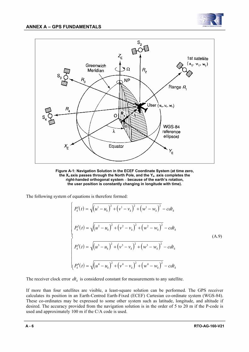
ANNEX A – GPS FUNDAMENTALS

A - 6 RTO-AG-160-V21

Figure A-1: Navigation Solution in the ECEF Coordinate System (at time zero, the Xe axis passes through the North Pole, and the Ye. axis completes the

right-handed orthogonal system – because of the earth’s rotation, the user position is constantly changing in longitude with time).

The following system of equations is therefore formed:

( ) ( ) ( ) ( )

( ) ( ) ( ) ( )

( ) ( ) ( ) ( )

( ) ( ) ( ) ( )

P t u u v v w w cdt

P t u u v v w w cdt

P t u u v v w w cdt

P t u u v v w w cdt

k k k k k

k k k k k

k k k k k

k k k k k

1 1 2 1 2 1 2

2 2 2 2 2 2 2

3 3 2 3 2 3 2

4 4 2 4 2 4 2

= − + − + − −

= − + − + − −

= − + − + − −

= − + − + − −

(A.9)

The receiver clock error dtk is considered constant for measurements to any satellite.

If more than four satellites are visible, a least-square solution can be performed. The GPS receiver calculates its position in an Earth-Centred Earth-Fixed (ECEF) Cartesian co-ordinate system (WGS-84). These co-ordinates may be expressed to some other system such as latitude, longitude, and altitude if desired. The accuracy provided from the navigation solution is in the order of 5 to 20 m if the P-code is used and approximately 100 m if the C/A code is used.

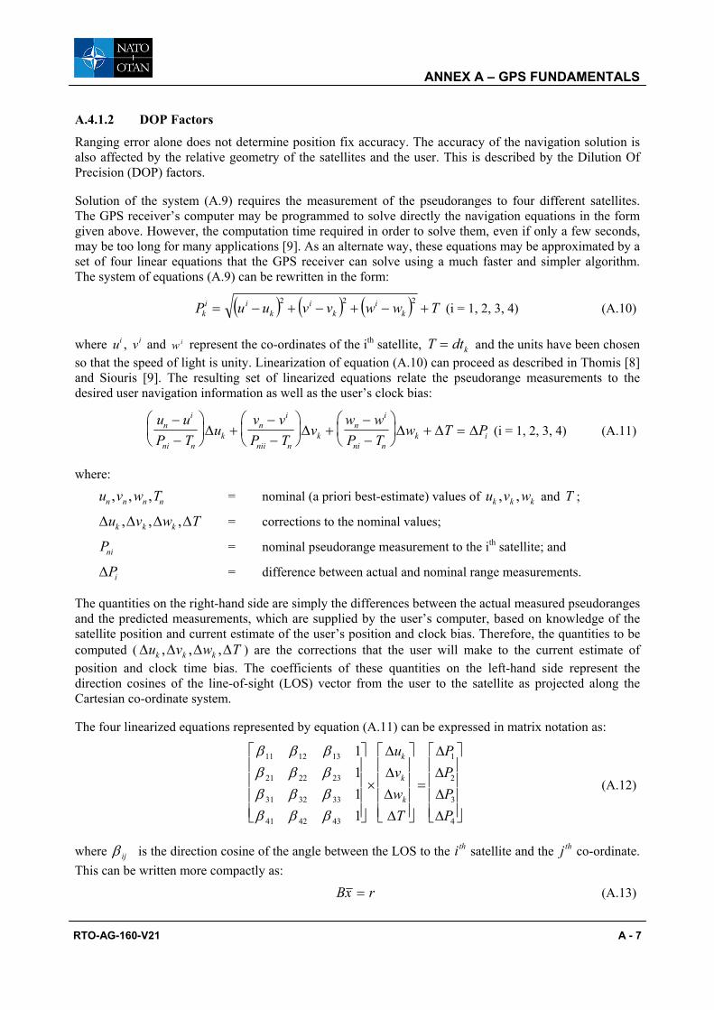
ANNEX A – GPS FUNDAMENTALS

RTO-AG-160-V21 A - 7

A.4.1.2 DOP Factors

Ranging error alone does not determine position fix accuracy. The accuracy of the navigation solution is also affected by the relative geometry of the satellites and the user. This is described by the Dilution Of Precision (DOP) factors.

Solution of the system (A.9) requires the measurement of the pseudoranges to four different satellites. The GPS receiver’s computer may be programmed to solve directly the navigation equations in the form given above. However, the computation time required in order to solve them, even if only a few seconds, may be too long for many applications [9]. As an alternate way, these equations may be approximated by a set of four linear equations that the GPS receiver can solve using a much faster and simpler algorithm. The system of equations (A.9) can be rewritten in the form:

( ) ( ) ( ) TwwvvuuP ki

ki

kii

k +−+−+−=222

(i = 1, 2, 3, 4) (A.10)

where ui , vi and w i represent the co-ordinates of the ith satellite, T dtk= and the units have been chosen so that the speed of light is unity. Linearization of equation (A.10) can proceed as described in Thomis [8] and Siouris [9]. The resulting set of linearized equations relate the pseudorange measurements to the desired user navigation information as well as the user’s clock bias:

u uP T

uv vP T

vw wP T

w T Pni

ni nk

ni

nii nk

ni

ni nk i

−−

+

−−

+

−−

+ =∆ ∆ ∆ ∆ ∆ (i = 1, 2, 3, 4) (A.11)

where:

u v w Tn n n n, , , = nominal (a priori best-estimate) values of u v wk k k, , and T ;

∆ ∆ ∆ ∆u v w Tk k k, , , = corrections to the nominal values;

Pni = nominal pseudorange measurement to the ith satellite; and

∆Pi = difference between actual and nominal range measurements.

The quantities on the right-hand side are simply the differences between the actual measured pseudoranges and the predicted measurements, which are supplied by the user’s computer, based on knowledge of the satellite position and current estimate of the user’s position and clock bias. Therefore, the quantities to be computed (∆ ∆ ∆ ∆u v w Tk k k, , , ) are the corrections that the user will make to the current estimate of position and clock time bias. The coefficients of these quantities on the left-hand side represent the direction cosines of the line-of-sight (LOS) vector from the user to the satellite as projected along the Cartesian co-ordinate system.

The four linearized equations represented by equation (A.11) can be expressed in matrix notation as:

β β ββ β ββ β ββ β β

11 12 13

21 22 23

31 32 33

41 42 43

1

2

3

4

1111

×

=

∆∆∆∆

∆∆∆∆

uvwT

PPPP

k

k

k (A.12)

where β ij is the direction cosine of the angle between the LOS to the ith satellite and the jth co-ordinate. This can be written more compactly as:

Bx r= (A.13)

ANNEX A – GPS FUNDAMENTALS

A - 8 RTO-AG-160-V21

where:

B = 4 × 4 solution matrix (i.e., matrix of coefficients of the linear equation);

x = user position and time correction vector ( [ ] )x u v w Tk k kT≡ ∆ ∆ ∆ ∆ ; and

r = pseudorange measurement difference vector ( [ ]r P P P P T≡ ∆ ∆ ∆ ∆1 2 3 4 ).

It is possible to estimate the covariance of the user position and time correction vector using the equation [10]:

( ) ( )cov covx B r B T= − −1 (A.14)

To a good approximation (i.e., assuming statistically independent random variables), Eq. (A.14) can be written as:

( ) ( )cov x B BT=−1

(A.15)

Assuming sufficient signal strength, this covariance matrix depends only on the direction and is no way dependent on the distances between the user and each satellite. The explicit form of the covariance matrix is:

( )cov x C

u uv uw ut

vu v vw vt

wu wv w wt

tu tv tw t

= =

σ σ σ σσ σ σ σσ σ σ σσ σ σ σ

2

2

2

2

(A.16)

The diagonal elements of this matrix are actually the variances of user position and time. The various DOP values are obtained as functions of the diagonal elements of the covariance matrix. Converting the Cartesian co-ordinates in matrix (2.16) to more convenient local geodetic co-ordinates, we have:

CLG

N NE NH

EN E EH

HN HE H

=

σ σ σσ σ σσ σ σ

2

2

2

(A.17)

Table A-1 shows the relationship between the DOP factors and the diagonal elements of the matrixes (A.16) and (A.17).

Table A-1: DOP Expressions

Vertical Vector (1d) VDOP = σH

Horizontal Vector (2d) HDOP = (σN2 + σE

2)1/2

Position Vector (3d) PDOP = (σN2 + σE

2 + σH2 )1/2

Time, clock offset vector (1d) TDOP = σt

Geometric, Position and Time Vector (4d) GDOP = (σN2 + σE

2 + σH2 + σt

2)1/2

ANNEX A – GPS FUNDAMENTALS

RTO-AG-160-V21 A - 9

It is also evident that:

PDOP HDOP VDOP= +2 2 (A.18)

GDOP PDOP TDOP= +2 2 (A.19)

The PDOP is very frequently used in navigation. This is because it directly relates error in GPS position to error in pseudo-range to the satellite. There is a proportionality between the PDOP (and GDOP) factor and the reciprocal value of the volume V of a particular tetrahedron formed by the satellites and the user position (Figure A-2).

Figure A-2: PDOP Tetrahedron. Four unit-vectors point toward the satellites and the ends of these vectors are connected with 6 line segments.

It is in fact demonstrated [11] that the PDOP is the RSS (i.e., square root of the sum of the squares) of the areas of the 4 faces of the tetrahedron, divided by its volume (i.e., the RSS of the reciprocals of the 4 altitudes of the tetrahedron). Therefore, we can write:

PDOPh h h hA B C D

= + + +1 1 1 1

2 2 2 2 (A.20)

At a particular time and location, the satellites 1, 2, 3, and 4 shown in Figure A-2, have determined elevations (°) and azimuths (°) with respect to the receiver. From these satellite positions the components (x, y, z) of the unit vectors to the satellites can be determined. Using the Pythagorean theorem, the distances between the ends of the unit vectors can be determined. Knowing these distances, a tetrahedron can be constructed (Figure A-3) and the four altitudes of the tetrahedron can be measured. Finally, using equation (A.20), the PDOP can be determined. There is no approximation associated with the geometric expression. Any residual error in PDOP determination is only due to construction of the tetrahedron and measurement of the altitudes. This method can be the basis for a computer algorithm designed to solve the 3-dimensional problem of PDOP determination.

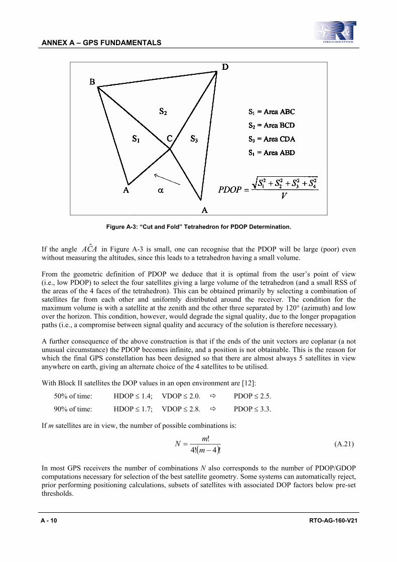
ANNEX A – GPS FUNDAMENTALS

A - 10 RTO-AG-160-V21

Figure A-3: “Cut and Fold” Tetrahedron for PDOP Determination.

If the angle ACA in Figure A-3 is small, one can recognise that the PDOP will be large (poor) even without measuring the altitudes, since this leads to a tetrahedron having a small volume.

From the geometric definition of PDOP we deduce that it is optimal from the user’s point of view (i.e., low PDOP) to select the four satellites giving a large volume of the tetrahedron (and a small RSS of the areas of the 4 faces of the tetrahedron). This can be obtained primarily by selecting a combination of satellites far from each other and uniformly distributed around the receiver. The condition for the maximum volume is with a satellite at the zenith and the other three separated by 120° (azimuth) and low over the horizon. This condition, however, would degrade the signal quality, due to the longer propagation paths (i.e., a compromise between signal quality and accuracy of the solution is therefore necessary).

A further consequence of the above construction is that if the ends of the unit vectors are coplanar (a not unusual circumstance) the PDOP becomes infinite, and a position is not obtainable. This is the reason for which the final GPS constellation has been designed so that there are almost always 5 satellites in view anywhere on earth, giving an alternate choice of the 4 satellites to be utilised.

With Block II satellites the DOP values in an open environment are [12]:

50% of time: HDOP ≤ 1.4; VDOP ≤ 2.0. PDOP ≤ 2.5.

90% of time: HDOP ≤ 1.7; VDOP ≤ 2.8. PDOP ≤ 3.3.

If m satellites are in view, the number of possible combinations is:

( )!4!4!−

=mmN (A.21)

In most GPS receivers the number of combinations N also corresponds to the number of PDOP/GDOP computations necessary for selection of the best satellite geometry. Some systems can automatically reject, prior performing positioning calculations, subsets of satellites with associated DOP factors below pre-set thresholds.

ANNEX A – GPS FUNDAMENTALS

RTO-AG-160-V21 A - 11

A.4.2 Carrier Phase The carrier phase observable is the difference between the received satellite carrier phase and the phase of the carrier generated by the receiver oscillator. The same error sources that affect pseudoranges, are responsible for the errors which determine the positional accuracy achieved with carrier phases [5]. Clearly, the mathematical formulation of any specific error component is different from the pseudorange case (i.e., phase measurement errors instead of range measurement errors). Since the antenna cannot sense the number of whole carrier waves between the satellite and the receiver (Integer Ambiguity), an extra parameter is inserted in the carrier phase equation:

( ) ( ) ( ) ( ) ( )

( ) ( ) ( )

Φ Φ Φ Φ

Φ Φ Φ Φ

kp

kp

kp

kp

kp

k kp p

t t N I tfc

T t

d t d t d t

= − + + −

+ + + +

1 ,

, , ε (A.22)

The symbols ( )Φk t and ( )Φp t denote the phase of the receiver generated signal and the phase of the satellite signal respectively, at the epoch t of satellite signal reception. The symbol ( )Nk

p 1 denotes the initial integer ambiguity. The terms ( )I tk

p,Φ and ( )T tk

p are the ionospheric and tropospheric delays. The ionospheric delay factor has a negative value because the carrier phase progresses when travelling through the ionosphere [5]. Furthermore, the tropospheric factor is converted in cycles using the factor f / c, where f is the nominal frequency and c is the speed of light in vacuum. The symbols ( )d tk ,Φ and ( )d tk

p

refer to the receiver and satellite hardware delays respectively. The symbol dkp,Φ denotes the multipath

effect and εΦ denotes the carrier phase measurement noise [5]. Assuming synchronisation of the satellite and receiver clocks, omitting other error sources (receiver phase tracking circuits, local oscillator, multipath and measurement noise), and taking into account both the time of transmission and reception of the signal, the equation for the phase observation between a satellite i and a receiver A, can be written as follows [13]:

( ) ( ) ( )Φ Φ ΦAi i

Atτ τ= − (A.23)

where:

( )ΦAi τ = phase reading (phase at receiver A of the signal from satellite i at time τ);

( )Φi t = received signal (phase of the signal as it left the satellite at time t); and ( )ΦA τ = generated signal phase (phase of the receiver’s signal at time τ).

If ( )ρAi t is the range between receiver and satellite, we have:

( )

tt

cAi

= −τρ

(A.24)

Therefore:

( )( )

( )( ) ( )

( )( )

Φ Φ ΦΦ

Φi i Ai

ii

Ai

i Ai

tt

ct

dtf

tc

ft

c= −

= − × + = − +τ

ρτ

∂ ρτ

ρ... ... (A.25)

And finally:

( ) ( ) ( ) ( )Φ Φ ΦAi i

Ai

A Aif

ct Nτ τ ρ τ= − − + (A.26)

ANNEX A – GPS FUNDAMENTALS

A - 12 RTO-AG-160-V21

where: ( )ΦA

i τ = phase reading (degree or cycles);

( )Φi τ = emitted signal;

( )fc

tAiρ = total number of wavelengths;

( )ΦA τ = generated signal;

N Ai = integer ambiguity;

f = frequency of the carrier; and c = speed of light.

The carrier phase measurement technique typically uses the difference between the carrier phases measured at a reference receiver and a user receiver. Particularly, a double-difference technique is used to remove the satellite and receiver clock errors. This is therefore an inherently differential GPS technique, which is discussed in Chapter 2 of this Thesis.

A.4.3 Doppler Observable The equation that associates the transmitted frequency from the satellite with the received frequency is:

ff

rc

k

p

=+1

' (A.27)

where f k is the received frequency, f p denotes the emitted frequency from the satellite, r’ denotes the radial velocity in the satellite-receiver direction and c denotes the speed of light in vacuum. The Doppler frequency shift is given by the difference f p – f k .

The radial velocity r’ is the actual rate of change in the satellite-receiver distance and it is given by:

rf f

fck

p

k

' = −−

⋅ (A.28)

The integrated Doppler count between two epochs t1 and t2 is given by:

( )N f f dtt tp

kt

t

( , )1 2

1

2

= −∫ (A.29)

More information about the Doppler Observable can be found in the literature [4].

A.5 GPS ERROR SOURCES

In this section the most important errors that affect pseudorange and carrier phase measurements are presented in some detail. These errors can be classified into the four broad categories listed below:

• Receiver Dependent Errors: • Clock Error; and • Noise and Resolution.

ANNEX A – GPS FUNDAMENTALS

RTO-AG-160-V21 A - 13

• Ephemeris Prediction Errors.

• Satellite Dependent Errors: • Clock Offset; and • Group Delays.

• Propagation Errors: • Ionospheric Delay; • Tropospheric Delay; and • Multipath.

Moreover, there are other errors to be taken into account, which are related to the User Dynamics. All of these errors are described in the following paragraphs.

A.5.1 Receiver Clock Error Most receivers have quartz clocks to measure the GPS time, which are not as accurate as the atomic clocks of the satellites. Therefore, there is an offset between the receiver and satellite clocks called Receiver Clock Error. This error affects both the measurement of the signal flight time and the calculation of the satellite’s position at time of transmission.

A.5.2 Receiver Noise and Resolution The receiver hardware and software design directly affect signal tracking and decoding of the navigation message. Measurement Noise is a random error, which depends entirely on the electronic components of the receiver. Receivers for very precise measurements are designed to minimise this error component. Both noise and resolution errors can be reduced by using appropriate filtering techniques. Theoretically, receiver noise can be removed by averaging the measurements, but only over fairly long periods of observation time.

A.5.3 Ephemeris Prediction Errors The ephemeris data are required for both pseudorange and phase computations. These errors are due to incorrect estimation of the satellites ephemeris at the MCS. A model for evaluating the errors (Figure A-4) is obtained by considering the three components of the vector representing the difference between estimated and true distance: ATK (along track), XTK (cross track), and RAD (radial).

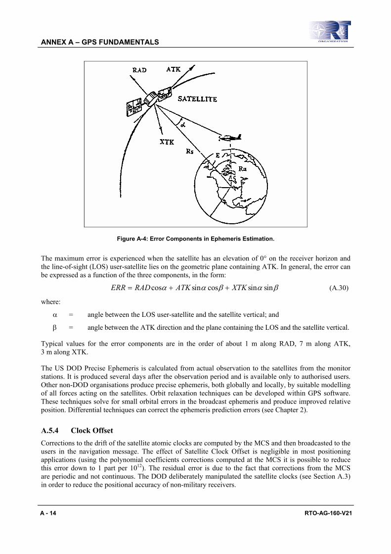
ANNEX A – GPS FUNDAMENTALS

A - 14 RTO-AG-160-V21

Figure A-4: Error Components in Ephemeris Estimation.

The maximum error is experienced when the satellite has an elevation of 0° on the receiver horizon and the line-of-sight (LOS) user-satellite lies on the geometric plane containing ATK. In general, the error can be expressed as a function of the three components, in the form:

ERR RAD ATK XTK= + +cos sin cos sin sinα α β α β (A.30)

where:

α = angle between the LOS user-satellite and the satellite vertical; and

β = angle between the ATK direction and the plane containing the LOS and the satellite vertical.

Typical values for the error components are in the order of about 1 m along RAD, 7 m along ATK, 3 m along XTK.

The US DOD Precise Ephemeris is calculated from actual observation to the satellites from the monitor stations. It is produced several days after the observation period and is available only to authorised users. Other non-DOD organisations produce precise ephemeris, both globally and locally, by suitable modelling of all forces acting on the satellites. Orbit relaxation techniques can be developed within GPS software. These techniques solve for small orbital errors in the broadcast ephemeris and produce improved relative position. Differential techniques can correct the ephemeris prediction errors (see Chapter 2).

A.5.4 Clock Offset Corrections to the drift of the satellite atomic clocks are computed by the MCS and then broadcasted to the users in the navigation message. The effect of Satellite Clock Offset is negligible in most positioning applications (using the polynomial coefficients corrections computed at the MCS it is possible to reduce this error down to 1 part per 1012). The residual error is due to the fact that corrections from the MCS are periodic and not continuous. The DOD deliberately manipulated the satellite clocks (see Section A.3) in order to reduce the positional accuracy of non-military receivers.

ANNEX A – GPS FUNDAMENTALS

RTO-AG-160-V21 A - 15

A.5.5 Group Delays These are the delays typical of the satellite electronic circuits. They are estimated on the ground before the satellites are launched and corrections are included in the navigation message.

A.5.6 Ionospheric Delay As the satellite signal passes through the ionosphere, it is delayed for two reasons [14]. Firstly, because it travels through a non-vacuum material (propagation delay); thus the Pseudo Random Noise (PRN) codes are delayed, while the carrier phase is advanced when passing through the ionosphere layers. Secondly, because it bends due to refraction; for many applications, the error caused by the bending effect can be considered negligible if the signals are transmitted by satellites with an elevation of 15° or more.

The ionospheric delay is dependent primarily on the number of electrons that the signal encounters along its propagation path. It is therefore dependent both on the ionosphere characteristics (variable during the day and with seasons), and the path angle (elevation angle of the satellite). It is possible to approximately evaluate the ionospheric delay using the following equation [14]:

∆τ = 40 31 2.TECcf

(A.31)

where TEC (Total Electron Content) express the electron density (electr./m2) of an ideal column with section 1 m2 and the symmetry axis coincident with the propagation path.

The expression for calculating the delay as a function of the elevation angle is the following [14]:

∆τ =0 53. ( )Z El

c (A.32)

where Z(El) is the obliquity factor.

Depending on the receiver design, different models can be adopted to calculate the correction terms to be applied to the pseudorange before solving the navigation equations. Particularly, C/A code receivers (L1 only), use a sinusoidal model of the ionosphere, derived from statistical studies (Klobuchar model), which take into account the variations of the ionospheric layers (low over night, rapidly getting higher after dawn, getting slightly higher during the afternoon and rapidly getting lower after sunset). The sinusoidal parameters (amplitude and period) are transmitted in the navigation message.

The relevant equations are the following:

( )

IDV DC AtP

= +−

cos

2π Φ (day) (A.33)

IDV DC= (night) (A.34)

where IDV (Ionospheric Vertical Delay) is expressed in nsec, DC is the constant night-day offset (5 nsec), A is the amplitude (whose value is between 10 and 100 nsec), Φ is the constant phase offset (14.00 hours), t is the local time, and P is the period.

The two factors A and P are transmitted as coefficients of a cubic equation representing a model of the ionosphere with varying latitude. The delay also depends on obliquity of the path and, therefore, elevation is included as an additional factor in the equation:

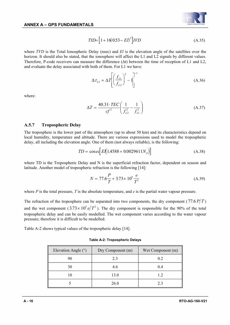
ANNEX A – GPS FUNDAMENTALS

A - 16 RTO-AG-160-V21

( )[ ]TID El IVD= + −1 16 053 3. (A.35)

where TVD is the Total Ionospheric Delay (nsec) and El is the elevation angle of the satellites over the horizon. It should also be stated, that the ionosphere will affect the L1 and L2 signals by different values. Therefore, P-code receivers can measure the difference (∆t) between the time of reception of L1 and L2, and evaluate the delay associated with both of them. For L1 we have:

∆ ∆τ LL

LT

ff1

1

2

2 1

1=

−

−

(A.36)

where:

−

⋅=∆ 2

122

2

1131.40

LL ffcfTECT (A.37)

A.5.7 Tropospheric Delay The troposphere is the lower part of the atmosphere (up to about 50 km) and its characteristics depend on local humidity, temperature and altitude. There are various expressions used to model the tropospheric delay, all including the elevation angle. One of them (not always reliable), is the following:

( )[ ]TD ec El NS= +cos . .14588 0 0029611 (A.38)

where TD is the Tropospheric Delay and N is the superficial refraction factor, dependent on season and latitude. Another model of tropospheric refraction is the following [14]:

NPT

eT

= + ×77 6 373 1052. . (A.39)

where P is the total pressure, T is the absolute temperature, and e is the partial water vapour pressure.

The refraction of the troposphere can be separated into two components, the dry component ( 77 6. P T ) and the wet component ( 373 105 2. × e T ). The dry component is responsible for the 90% of the total tropospheric delay and can be easily modelled. The wet component varies according to the water vapour pressure; therefore it is difficult to be modelled.

Table A-2 shows typical values of the tropospheric delay [14].

Table A-2: Tropospheric Delays

Elevation Angle (°) Dry Component (m) Wet Component (m)

90 2.3 0.2

30 4.6 0.4

10 13.0 1.2

5 26.0 2.3

ANNEX A – GPS FUNDAMENTALS

RTO-AG-160-V21 A - 17

A.5.8 Multipath GPS signals may arrive at the receiver antenna via different paths, due to reflections by objects along the path. Such effect is known as multipath. The reflected signal will have a different path length compared to the direct signal; therefore it will give a biased distance measurement. Multipath depends on the surrounding environment of the receiver and the satellite geometry. Generally, multipath will be greater for low elevation satellites. For surveying applications, the antenna ground plane prevents the reflected signal from the ground to reach the antenna phase centre [14]. Code multipath is much greater than carrier phase multipath; and the C/A code multipath error is greater than the P code one [15]. Multipath can be modelled only at static points, by taking observations at the same points, at the same hour on consecutive days. This, however, is not practical or even impossible in a dynamic environment. Other interesting techniques use the Signal to Noise Ratio (SNR) to detect and quantify multipath [16].

A.5.9 User Dynamics Errors There are various errors associated with a dynamic GPS platform. These errors range from the physical masking of the GPS antenna to the accuracy degradation caused by sudden acceleration of the antenna. If carrier phase is used, the resulting effect of “cycle slips” is the need for re-initialisation (i.e., re-determination of the integer ambiguities). In general, a distinction is made between medium-low and high dynamic platforms. Due to the scope of the present dissertation, we will investigate the effect of high dynamic aircraft manoeuvres on GPS performance.

A.6 UERE VECTOR

The User Equivalent Range Error (UERE) is an error vector along the line-of-sight user-satellite given by the projection of all system errors. The value of this vector can be reduced only by careful design of the receiver, since there is nothing the user can do to reduce other error sources. The UERE is generally measured in metres (95%).

The portion of the UERE allocated to the space and control segments is called the User Range Error (URE) and is defined at the phase centre of the satellite antenna. The portion of the UERE allocated to the User Equipment is called the UE Error (UEE). Specifically, the UERE is the root-sum-square of the URE and UEE. Typical values of the UERE vector are in the order of 13 m (95%) for P-code receivers and 15.7 to 23.1 m (95%) for C/A code receivers.

A.7 GPS AND KALMAN FILTERING

The GPS measurement process is corrupted by noise that introduces errors into the calculation. This noise includes the errors in the ionospheric corrections and system dynamics not considered during the measurement process (e.g., user clock drift). A Kalman filter characterises the noise sources in order to minimise their effect on the desired receiver outputs.

The Kalman filter is a linear, recursive estimator that produces the minimum variance estimate in a least square sense under the assumption of white, Gaussian noise processes. There are two basic processes that are modelled by a Kalman filter. The first process is a model describing how the error state vector changes in time (system dynamics model). The second model defines the relationship between the error state vector and any measurements processed by the filter (measurement model).

The Kalman filter sorts out information and weights the relative contributions of the measurements and of the dynamic behaviour of the state vector. The measurements and state vector are weighted by their respective covariance matrices. If the measurements are inaccurate (large variances) when compared to the

ANNEX A – GPS FUNDAMENTALS

A - 18 RTO-AG-160-V21

state vector estimate, then the filter will de-weight the measurements. On the other hand, if the measurements are very accurate (small variances) when compared to the state vector estimate, then the filter will tend to weight the measurements heavily with the consequence that its previously computed state estimate will contribute little to the latest state estimate.

When the GPS receiver is aided or integrated with other navigation sensors (e.g., an Inertial Navigation System, an external clock or an altimeter), then the Kalman filter can be extended to include the measurements added by these sensors. In fact, a typical implementation for integrated systems would be to have a central Kalman filter incorporating measurements from all available sources. More detailed information about Kalman filters for GPS receivers and GPS-based integrated navigation systems can be found in the literature [9].

A.8 GPS MODERNIZATION

Current GPS Modernization efforts focus on improving position and timing accuracy, availability, integrity monitoring support capability and enhancement to the control system. As these system enhancements are introduced, users will be able to continue to use existing receivers, as signal backward compatibility is an absolute requirement for both the military and civil user communities. Although current GPS users will be able to operate at the same, or better, levels of performance that they enjoy today, users will need to modify existing user equipment or procure new user equipment in order to take full advantage of any new signal structure enhancements [17].

GPS modernization is a multi-phase effort to be executed over the next 15 years. Additional signals are planned to enhance the ability of GPS to support civil users and provide a new military code. The first new signal will be the C/A code on the L2 frequency (1227.60 MHz). This feature will enable dual channel civil receivers to correct for ionospheric error. A third civil signal will be added on the L5 frequency (1176.45 MHz) for use in safety-of-life applications. L5 can serves as a redundant signal to the GPS L1 frequency (1575.42 MHz) with a goal of assurance of continuity of service potentially to provide precisions approach capability for aviation users. In addition, a secure and spectrally separated Military Code (M-Code) will be broadcast on the L1 and L2 frequencies enabling the next generation of military receivers to operate more fully in an electronic jamming environment. At least one satellite is planned to be operational on orbit with the new C/A on L2 and M-Code capability no later than 2003. The Initial Operating Capability (IOC) with 18 satellites on orbit is planned for 2008 and the Full Operational Capability (FOC) with 24 satellites on orbit is planned for 2010. At least one satellite is planned to be operational on orbit with the new L5 capability no later than 2005, with IOC planned for 2012 and FOC planned for 2014 [18].

A.9 REFERENCES

[1] Parkinson, B.W. and Spilker, J.J., Jr. Editors. (1996). “Global Positioning System: Theory and Applications – Volumes I and II”. Progress in Astronautics and Aeronautics. Vol. 163. Published by the American Institute of Aeronautics and Astronautics (AIAA).

[2] Kayton, M. and Fried, W.R. (1997). “Avionics Navigation Systems”. Second Edition. Wiley Interscience Publication.

[3] Kaplan, E.D. (Editor). (1996). “Understanding GPS Principles and Applications”. Artech House Publishers, New York (USA).

[4] Seeber, G. (1994). “Satellite Geodesy”. Second Edition. Artech House Publishers, New York (USA).

ANNEX A – GPS FUNDAMENTALS

RTO-AG-160-V21 A - 19

[5] Leick, A. (1995). “GPS Satellite Surveying”. Second Edition. Department of Surveying Engineering – University of Maine (USA).

[6] AGARD LS-161. (1990). “The NAVSTAR GPS System”. NATO Advisory Group for Aerospace Research and Development. Neuilly-sur-Seine (France).

[7] ASHTECH Inc. (1996). “ASHTECH Z-12 Receiver”. Technical Specification Leaflet.

[8] Thomis, D.M. (1984). “Global Positioning System – A Modification to the Baseline Satellite Constellation for Improved Geometric Performance”. US Air Force Institute of Technology.

[9] Siouris, G.M. (1993). “Aerospace Avionics Systems”. Academic Press, San Diego, California (USA).

[10] Maybeck, P.S. (1979). “Stochastic Models, Estimation, and Control”. Vol. I, Academic Press, New York (USA).

[11] Philips, A.H. (1990). “The Determination of PDOP in GPS”. AGARD-AG-314. NATO Advisory Group for Aerospace Research and Development. Neuilly-sur-Seine (France).

[12] Vagias, C. (1995). “High Precision Differential GPS Using New Hardware”. MSc Dissertation. Institute of Engineering Surveying and Space Geodesy (IESSG) – University of Nottingham.

[13] Ashkenazi, V. (1997). “Principles of GPS and Observables”. MSc Lecture Notes. Institute of Engineering Surveying and Space Geodesy (IESSG) – University of Nottingham.

[14] Dodson, A.H. (2002). “Propagation Effects on GPS Measurements”. MSc Lecture Notes. Institute of Engineering Surveying and Space Geodesy (IESSG) – University of Nottingham.

[15] Walsh, D. (1994). “Kinematic GPS Ambiguity Resolution”. PhD Thesis. Institute of Engineering Surveying and Space Geodesy (IESSG) – University of Nottingham.

[16] Adham, T.A. (1995). “Multipath Effects on Carrier Phase”. MSc Dissertation. Institute of Engineering Surveying and Space Geodesy (IESSG) – University of Nottingham.

[17] Dye, S. and Baylin, F. (2004). “The GPS Manual Principles and Applications”. Second Edition. Baylin Publications (USA).

[18] US Department of Defense and US Department of Transportation. (2001). “Federal Radionavigation Plan – 2001”. National Technical Information Services. Springfield (VA). Doc. DOT-VNTSC-RSPA-01-3/DOD-4650.5.

ANNEX A – GPS FUNDAMENTALS

A - 20 RTO-AG-160-V21

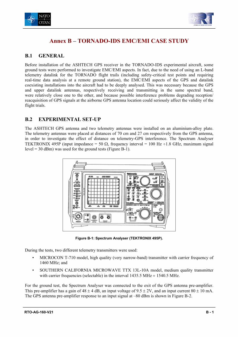
RTO-AG-160-V21 B - 1

Annex B – TORNADO-IDS EMC/EMI CASE STUDY

B.1 GENERAL

Before installation of the ASHTECH GPS receiver in the TORNADO-IDS experimental aircraft, some ground tests were performed to investigate EMC/EMI aspects. In fact, due to the need of using an L-band telemetry datalink for the TORNADO flight trails (including safety-critical test points and requiring real-time data analysis at a remote ground station), the EMC/EMI aspects of the GPS and datalink coexisting installations into the aircraft had to be deeply analysed. This was necessary because the GPS and upper datalink antennas, respectively receiving and transmitting in the same spectral band, were relatively close one to the other, and because possible interference problems degrading reception/ reacquisition of GPS signals at the airborne GPS antenna location could seriously affect the validity of the flight trials.

B.2 EXPERIMENTAL SET-UP

The ASHTECH GPS antenna and two telemetry antennas were installed on an aluminium-alloy plate. The telemetry antennas were placed at distances of 70 cm and 27 cm respectively from the GPS antenna, in order to investigate the effect of distance on telemetry-GPS interference. The Spectrum Analyser TEKTRONIX 495P (input impedance = 50 Ω, frequency interval = 100 Hz ÷1.8 GHz, maximum signal level = 30 dBm) was used for the ground tests (Figure B-1).

Figure B-1: Spectrum Analyser (TEKTRONIX 495P).

During the tests, two different telemetry transmitters were used:

• MICROCON T-710 model, high quality (very narrow-band) transmitter with carrier frequency of 1460 MHz; and

• SOUTHERN CALIFORNIA MICROWAVE TTX 13L-10A model, medium quality transmitter with carrier frequencies (selectable) in the interval 1435.5 MHz ÷ 1540.5 MHz.

For the ground test, the Spectrum Analyser was connected to the exit of the GPS antenna pre-amplifier. This pre-amplifier has a gain of 48 ± 4 dB, an input voltage of 9.5 ± 2V, and an input current 80 ± 10 mA. The GPS antenna pre-amplifier response to an input signal at –80 dBm is shown in Figure B-2.

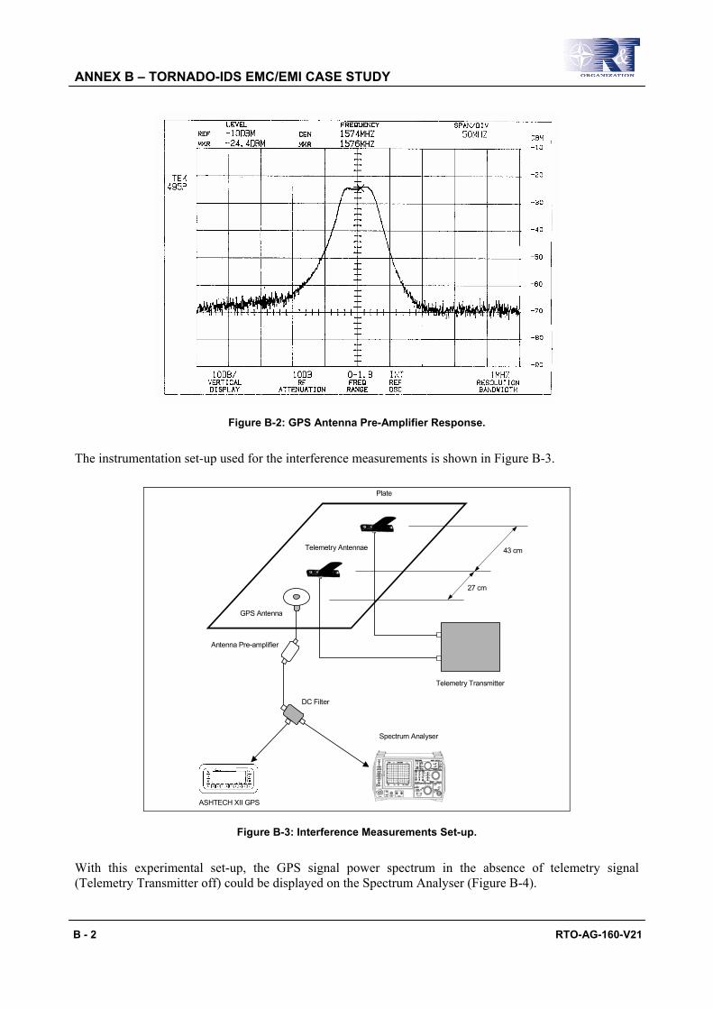
ANNEX B – TORNADO-IDS EMC/EMI CASE STUDY

B - 2 RTO-AG-160-V21

Figure B-2: GPS Antenna Pre-Amplifier Response.

The instrumentation set-up used for the interference measurements is shown in Figure B-3.

Telemetry Antennae

DC Filter

Spectrum Analyser

27 cm

43 cm

ASHTECH XII GPS

Antenna Pre-amplifier

Telemetry Transmitter

GPS Antenna

Plate

Figure B-3: Interference Measurements Set-up.

With this experimental set-up, the GPS signal power spectrum in the absence of telemetry signal (Telemetry Transmitter off) could be displayed on the Spectrum Analyser (Figure B-4).

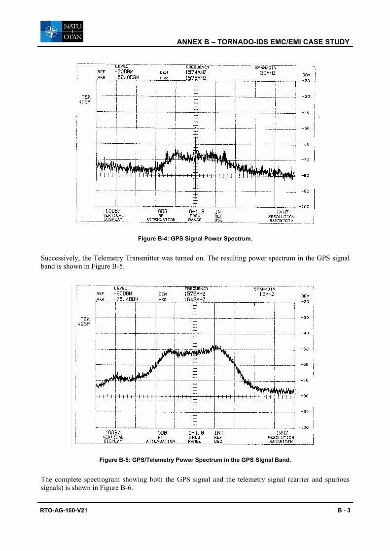
ANNEX B – TORNADO-IDS EMC/EMI CASE STUDY

RTO-AG-160-V21 B - 3

Figure B-4: GPS Signal Power Spectrum.

Successively, the Telemetry Transmitter was turned on. The resulting power spectrum in the GPS signal band is shown in Figure B-5.

Figure B-5: GPS/Telemetry Power Spectrum in the GPS Signal Band.

The complete spectrogram showing both the GPS signal and the telemetry signal (carrier and spurious signals) is shown in Figure B-6.

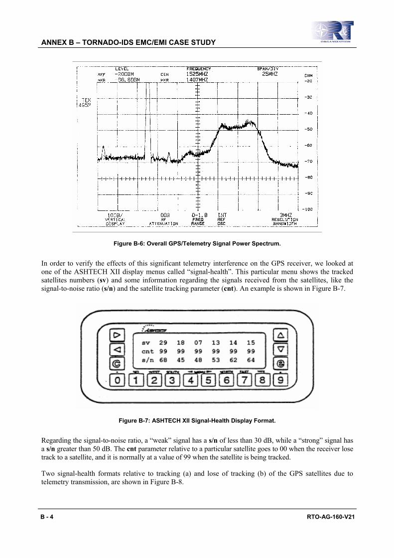
ANNEX B – TORNADO-IDS EMC/EMI CASE STUDY

B - 4 RTO-AG-160-V21

Figure B-6: Overall GPS/Telemetry Signal Power Spectrum.

In order to verify the effects of this significant telemetry interference on the GPS receiver, we looked at one of the ASHTECH XII display menus called “signal-health”. This particular menu shows the tracked satellites numbers (sv) and some information regarding the signals received from the satellites, like the signal-to-noise ratio (s/n) and the satellite tracking parameter (cnt). An example is shown in Figure B-7.

Figure B-7: ASHTECH XII Signal-Health Display Format.

Regarding the signal-to-noise ratio, a “weak” signal has a s/n of less than 30 dB, while a “strong” signal has a s/n greater than 50 dB. The cnt parameter relative to a particular satellite goes to 00 when the receiver lose track to a satellite, and it is normally at a value of 99 when the satellite is being tracked.

Two signal-health formats relative to tracking (a) and lose of tracking (b) of the GPS satellites due to telemetry transmission, are shown in Figure B-8.

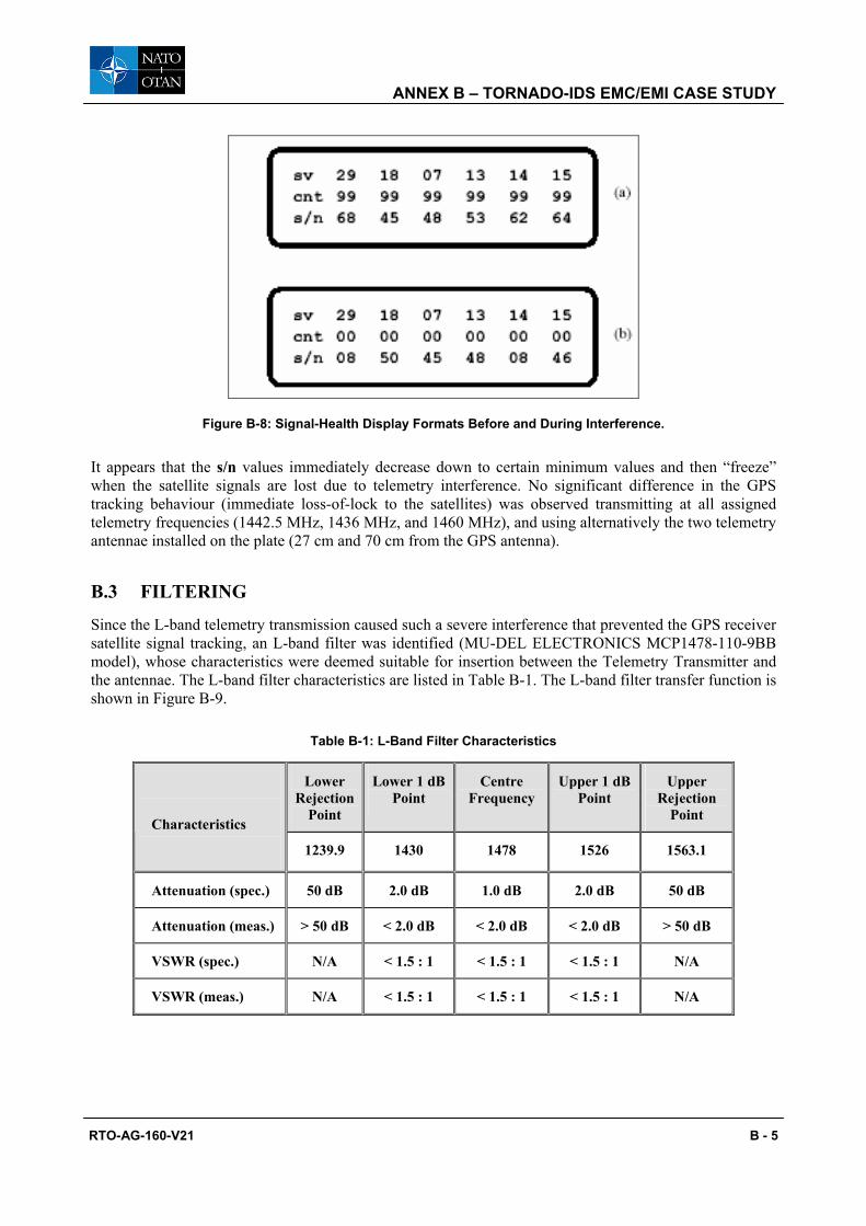
ANNEX B – TORNADO-IDS EMC/EMI CASE STUDY

RTO-AG-160-V21 B - 5

Figure B-8: Signal-Health Display Formats Before and During Interference.

It appears that the s/n values immediately decrease down to certain minimum values and then “freeze” when the satellite signals are lost due to telemetry interference. No significant difference in the GPS tracking behaviour (immediate loss-of-lock to the satellites) was observed transmitting at all assigned telemetry frequencies (1442.5 MHz, 1436 MHz, and 1460 MHz), and using alternatively the two telemetry antennae installed on the plate (27 cm and 70 cm from the GPS antenna).

B.3 FILTERING

Since the L-band telemetry transmission caused such a severe interference that prevented the GPS receiver satellite signal tracking, an L-band filter was identified (MU-DEL ELECTRONICS MCP1478-110-9BB model), whose characteristics were deemed suitable for insertion between the Telemetry Transmitter and the antennae. The L-band filter characteristics are listed in Table B-1. The L-band filter transfer function is shown in Figure B-9.

Table B-1: L-Band Filter Characteristics

Lower Rejection

Point

Lower 1 dB Point

Centre Frequency

Upper 1 dB Point

Upper Rejection

Point

Characteristics

1239.9 1430 1478 1526 1563.1

Attenuation (spec.) 50 dB 2.0 dB 1.0 dB 2.0 dB 50 dB

Attenuation (meas.) > 50 dB < 2.0 dB < 2.0 dB < 2.0 dB > 50 dB

VSWR (spec.) N/A < 1.5 : 1 < 1.5 : 1 < 1.5 : 1 N/A

VSWR (meas.) N/A < 1.5 : 1 < 1.5 : 1 < 1.5 : 1 N/A

ANNEX B – TORNADO-IDS EMC/EMI CASE STUDY

B - 6 RTO-AG-160-V21

Figure B-9: L-Band Filter Transfer Function.

The L-band filter attenuates the telemetry signal of about – 2 dBm, but it guarantees, based on the specs, an attenuation of 50 dBm at frequencies greater than 1563.1 MHz. Therefore, in principle, that filter could avoid interference at 1575.42 MHz (GPS L1 frequency). After installing the L-band filter between the Telemetry Transmitter and the antennae, further ground tests were performed.

Two GPS receiver signal-health formats recorded before (a) and after (b) activating the telemetry transmitter, are shown in Figure B-10.

Figure B-10: Signal-Health Display Formats with L-Band Filter.

It is evident that, from a practical point of view, the L-band filter significantly improved the GPS receiver performance, avoiding the interference problems previously found. In order to further investigate the effects of the L-band filter insertion on the L1 GPS signals tracked by the ASHTECH XII receiver, we also measured with the Spectrum Analyser the signal received by the GPS antenna. The results of these measures are shown in Figures B-11 and B-12.

ANNEX B – TORNADO-IDS EMC/EMI CASE STUDY

RTO-AG-160-V21 B - 7

Figure B-11: GPS/Telemetry Signal Spectrum in the GPS Signal Band (with Filter).

Figure B-12: Overall GPS/Telemetry Signal Spectrum (with Filter).

Both the GPS signal and the telemetry signal received by the GPS antenna did not show significant changes. The irregularity of the spectrum and the presence of picks are probably due to signal distortions, which may be caused, for instance, by the GPS antenna pre-amplifier. Unfortunately, the instrumentation available was not sufficient to test this hypothesis, since the level of the disturbance was comparable to the background noise. The telemetry signal spectrum with the L-band filter is almost unchanged, as shown in Figure B-13 (see Figure 5-9 in Chapter 5 for comparison).

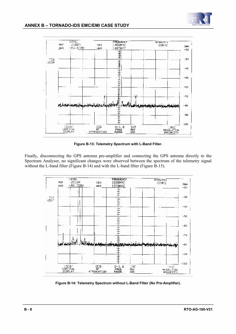
ANNEX B – TORNADO-IDS EMC/EMI CASE STUDY

B - 8 RTO-AG-160-V21

Figure B-13: Telemetry Spectrum with L-Band Filter.

Finally, disconnecting the GPS antenna pre-amplifier and connecting the GPS antenna directly to the Spectrum Analyser, no significant changes were observed between the spectrum of the telemetry signal without the L-band filter (Figure B-14) and with the L-band filter (Figure B-15).

Figure B-14: Telemetry Spectrum without L-Band Filter (No Pre-Amplifier).

ANNEX B – TORNADO-IDS EMC/EMI CASE STUDY

RTO-AG-160-V21 B - 9

Figure B-15: Telemetry Spectrum with L-Band Filter (No Pre-Amplifier).

Due to the positive results of the ground tests performed with the L-band filter MU-DEL ELECTRONICS mod. MCP1478-110-9BB, this filter was finally selected for installation on the TORNADO-IDS FTI system.

ANNEX B – TORNADO-IDS EMC/EMI CASE STUDY

B - 10 RTO-AG-160-V21

RTO-AG-160-V21 C - 1

Annex C – MB-339CD DGPS IN-FLIGHT INVESTIGATION

C.1 FLIGHT TEST PLANNING

Specific flight profiles were defined in order to allow a comparative evaluation of the TANS and ASHTECH XII receivers on the MB-339CD aircraft. Particularly, the following manoeuvres, representative of the real dynamics conditions that can be encountered during most flight tasks, were performed:

• Turns with constant bank angles;

• Dives followed by a pull up to 4 g’s along the four cardinal directions; and

• High dynamic manoeuvres as tonneau and stick-jerks.

The first type of manoeuvre was performed in order to evaluate the antenna masking effect. The second is a typical weapon-aiming manoeuvre, while the third type of manoeuvre was performed in order to obtain a rough estimation of the DGPS positioning accuracy. The last type of manoeuvre was performed in order to test the receivers in a high dynamic environment.

It must be underlined that a determination of the accuracies provided by two systems was not considered essential in this phase of the program and therefore it was not carried out in the MB-339CD test campaign. This was done for two good reasons.

• The availability of a copious literature concerning previous evaluations conducted of DGPS systems, confirmed the high accuracies declared by TRIMBLE and ASHTECH for the two systems under test. This was particularly true for straight-and-level flight conditions and low dynamic manoeuvres; and

• The difficulty of measuring the system accuracy during execution of flight trials. In order to prove that a DGPS system meet its accuracy requirements, an independent reference system is needed with an accuracy of at least 8 (preferably 10) times better. Moreover, the verification should be carried out over the full flight envelope. Systems that could be possibly used were cinetheodolites or laser trackers, with accuracies in the order of 0.2 – 0.5 metre RMS. However, neither cinetheodolites nor laser tracker facilities were available in this phase of the program.

C.2 FLIGHT DATA ANALYSIS

As expected, during straight-and-level flight both receivers under test performed satisfactorily, with no significant data losses recorded. However, during execution of dynamic manoeuvres both systems frequently lost lock to the satellites. Analysing the dynamics of the aircraft it was understood that this phenomenon could be due to shielding of the GPS antenna by the aircraft body (wings, fuselage and tails). Data analysis also showed that during dynamic manoeuvres both systems experienced a very significant increase of the PDOP factor. However, some remarkable differences were noted between the two receivers in terms of reacquisition time after data losses.

C.2.1 GPS Data Losses and Reacquisition The INS data (recorder by the FTI) relative to variations of significant flight parameters in a period of a few minutes (heading, altitude, pitch, bank, etc.) are shown in Figure C-1. Identification of the aircraft parameters, together with the various scales, is given in Table C-1.

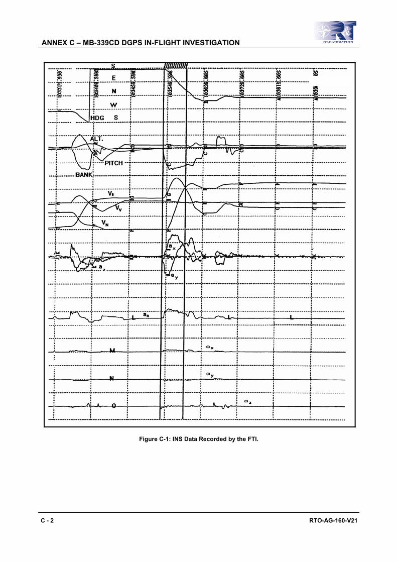
ANNEX C – MB-339CD DGPS IN-FLIGHT INVESTIGATION

C - 2 RTO-AG-160-V21

Figure C-1: INS Data Recorded by the FTI.

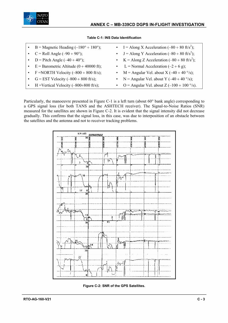
ANNEX C – MB-339CD DGPS IN-FLIGHT INVESTIGATION

RTO-AG-160-V21 C - 3

Table C-1: INS Data Identification

• B = Magnetic Heading (–180° ÷ 180°); • C = Roll Angle (–90 ÷ 90°); • D = Pitch Angle (–40 ÷ 40°); • E = Barometric Altitude (0 ÷ 40000 ft); • F =NORTH Velocity (–800 ÷ 800 ft/s); • G = EST Velocity (–800 ÷ 800 ft/s); • H =Vertical Velocity (–800÷800 ft/s);

• I = Along X Acceleration (–80 ÷ 80 ft/s2); • J = Along Y Acceleration (–80 ÷ 80 ft/s2); • K = Along Z Acceleration (–80 ÷ 80 ft/s2); • L = Normal Acceleration (–2 ÷ 6 g); • M = Angular Vel. about X (–40 ÷ 40 °/s); • N = Angular Vel. about Y (–40 ÷ 40 °/s); • O = Angular Vel. about Z (–100 ÷ 100 °/s).

Particularly, the manoeuvre presented in Figure C-1 is a left turn (about 60° bank angle) corresponding to a GPS signal loss (for both TANS and the ASHTECH receiver). The Signal-to-Noise Ratios (SNR) measured for the satellites are shown in Figure C-2. It is evident that the signal intensity did not decrease gradually. This confirms that the signal loss, in this case, was due to interposition of an obstacle between the satellites and the antenna and not to receiver tracking problems.

Figure C-2: SNR of the GPS Satellites.

ANNEX C – MB-339CD DGPS IN-FLIGHT INVESTIGATION

C - 4 RTO-AG-160-V21

The relative positions of the aircraft and satellites during the manoeuvre are shown in Figure C-3. It can be noticed that the aircraft body masked many of the satellites during the turn (starting from an initial heading of 180°). Signal reacquisition took place when the aircraft progressively reduced the bank angle and the heading variation rate.

224

26 16

19

90° E

75°

60°

45°

30°

15°0° 15°

30°

35°

20°

25° W 270°

255°

240°

225°

210°

195°180°

165°

150°

135°

120°

105°

90 80 70 6050 403020100

N

S

1827

Figure C-3: Relative Geometry of the Aircraft and Satellites.

Similar considerations can be done looking at the Figures C-4, C-5 and C-6 relative to a left turn with –45° bank angle. However, in this case, a difference was noticed between the two receivers. As the position of the aircraft longitudinal axes during the turn got closer to satellite 2 (in the horizontal plane) the TANS receiver experienced a loss of track to all satellites, while the satellites 19 and 27 were still tracked by the ASHTECH receiver. This was due to the internal processing of the receiver. In fact, the ASHTECH receiver was able to maintain track to the satellites in view (19 and 27) even when their SNRs were very low (i.e., below 5 dB), while in the same conditions TANS lost track to all satellites. This significantly reduced the time required by the ASHTECH receiver for a new position fix as soon as four satellites were available again. Other trials, performed with similar conditions, confirmed that with the ASHTECH receiver shorter periods were needed to compute a new positioning solution after loss of satellite signals.

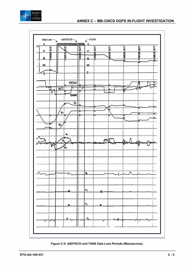
ANNEX C – MB-339CD DGPS IN-FLIGHT INVESTIGATION

RTO-AG-160-V21 C - 5

Figure C-4: ASHTECH and TANS Data Loss Periods (Manoeuvres).

ANNEX C – MB-339CD DGPS IN-FLIGHT INVESTIGATION

C - 6 RTO-AG-160-V21

Figure C-5: ASHTECH and TANS Data Loss Periods (SNRs).

ANNEX C – MB-339CD DGPS IN-FLIGHT INVESTIGATION

RTO-AG-160-V21 C - 7

2

26

16

19

90° E

75°

60°

45°

30°

15° 0° 15°

30°

35°

20°

25° W 270°

255°

240°

225°

210°

195°180°

165°

150°

135°

120°

105°

90 80 70 60 50 403020100

N

S

27

Figure C-6: Aircraft-Satellites Relative Geometry During Data Loss.

Figures C-7, C-8 and C-9 confirm that both the increase of PDOP (due to degradation of satellite-receiver geometry) and the progressive reduction of the SNRs during dynamic manoeuvres were responsible, together with masking of the GPS antenna, for the satellite signal losses in the TANS receiver. In this case, the TANS navigation data were lost with a small variation of the aircraft-receiver relative geometry, loss occurred with a small variation of the aircraft-receiver relative geometry, and no satellites were lost due to masking. The ASHTECH receiver, in the same conditions, did not experience any signal loss.

ANNEX C – MB-339CD DGPS IN-FLIGHT INVESTIGATION

C - 8 RTO-AG-160-V21

Figure C-7: TANS Data Loss Periods (Manoeuvres).

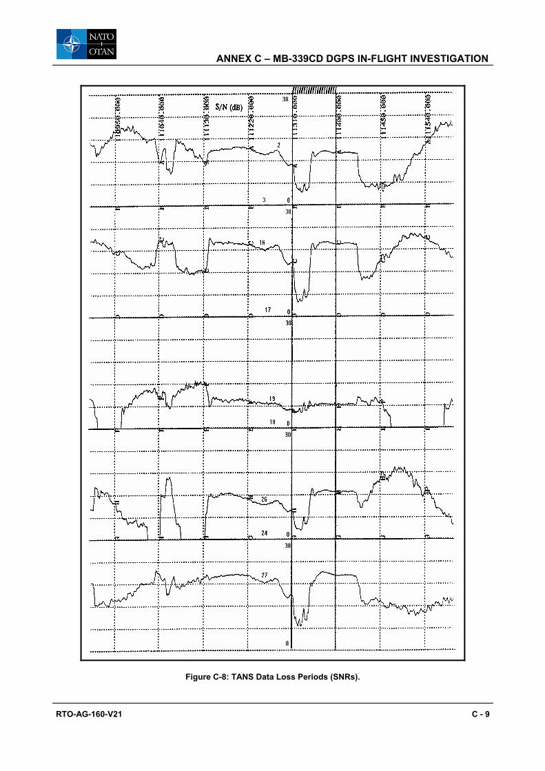
ANNEX C – MB-339CD DGPS IN-FLIGHT INVESTIGATION

RTO-AG-160-V21 C - 9

Figure C-8: TANS Data Loss Periods (SNRs).

ANNEX C – MB-339CD DGPS IN-FLIGHT INVESTIGATION

C - 10 RTO-AG-160-V21

2

26

1

1

90°

75

60

45

3015015

30

35

20

25 W

255

240

225

210

195 180 165

150

135

120

105

9080706050403020100

N

S

27

Figure C-9: Aircraft-Satellites Relative Geometry During TANS Data Loss.

Similar manoeuvres, performed in other directions, did not cause any problem to the receivers. An example is shown in the Figures C-10 and C-11 relative to a right turn at 40° bank, where some changes of satellite configuration occurred, but not signal losses.

2

3

1 190°

75

60

45

3015015

30

35

20

25 W

255

240

225

210195 180 165

150

135

120

105

9080706050403020100

N

S

27

24

18

Figure C-10: Aircraft-Satellites Relative Geometry (No Data Losses).

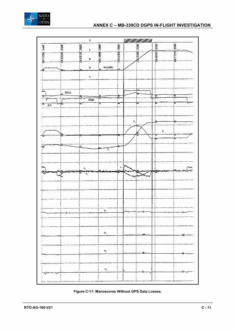
ANNEX C – MB-339CD DGPS IN-FLIGHT INVESTIGATION

RTO-AG-160-V21 C - 11

Figure C-11: Manoeuvres Without GPS Data Losses.

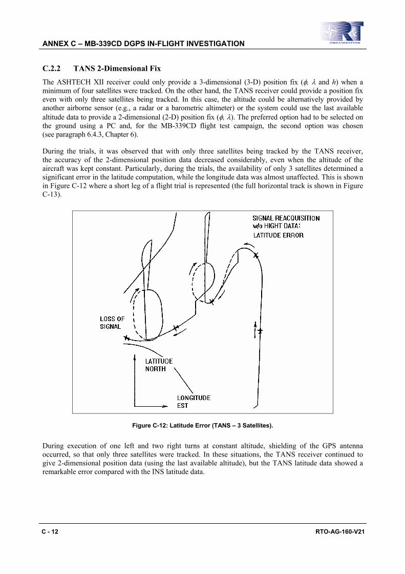
ANNEX C – MB-339CD DGPS IN-FLIGHT INVESTIGATION

C - 12 RTO-AG-160-V21

C.2.2 TANS 2-Dimensional Fix The ASHTECH XII receiver could only provide a 3-dimensional (3-D) position fix (φ, λ and h) when a minimum of four satellites were tracked. On the other hand, the TANS receiver could provide a position fix even with only three satellites being tracked. In this case, the altitude could be alternatively provided by another airborne sensor (e.g., a radar or a barometric altimeter) or the system could use the last available altitude data to provide a 2-dimensional (2-D) position fix (φ, λ). The preferred option had to be selected on the ground using a PC and, for the MB-339CD flight test campaign, the second option was chosen (see paragraph 6.4.3, Chapter 6).

During the trials, it was observed that with only three satellites being tracked by the TANS receiver, the accuracy of the 2-dimensional position data decreased considerably, even when the altitude of the aircraft was kept constant. Particularly, during the trials, the availability of only 3 satellites determined a significant error in the latitude computation, while the longitude data was almost unaffected. This is shown in Figure C-12 where a short leg of a flight trial is represented (the full horizontal track is shown in Figure C-13).

Figure C-12: Latitude Error (TANS – 3 Satellites).

During execution of one left and two right turns at constant altitude, shielding of the GPS antenna occurred, so that only three satellites were tracked. In these situations, the TANS receiver continued to give 2-dimensional position data (using the last available altitude), but the TANS latitude data showed a remarkable error compared with the INS latitude data.

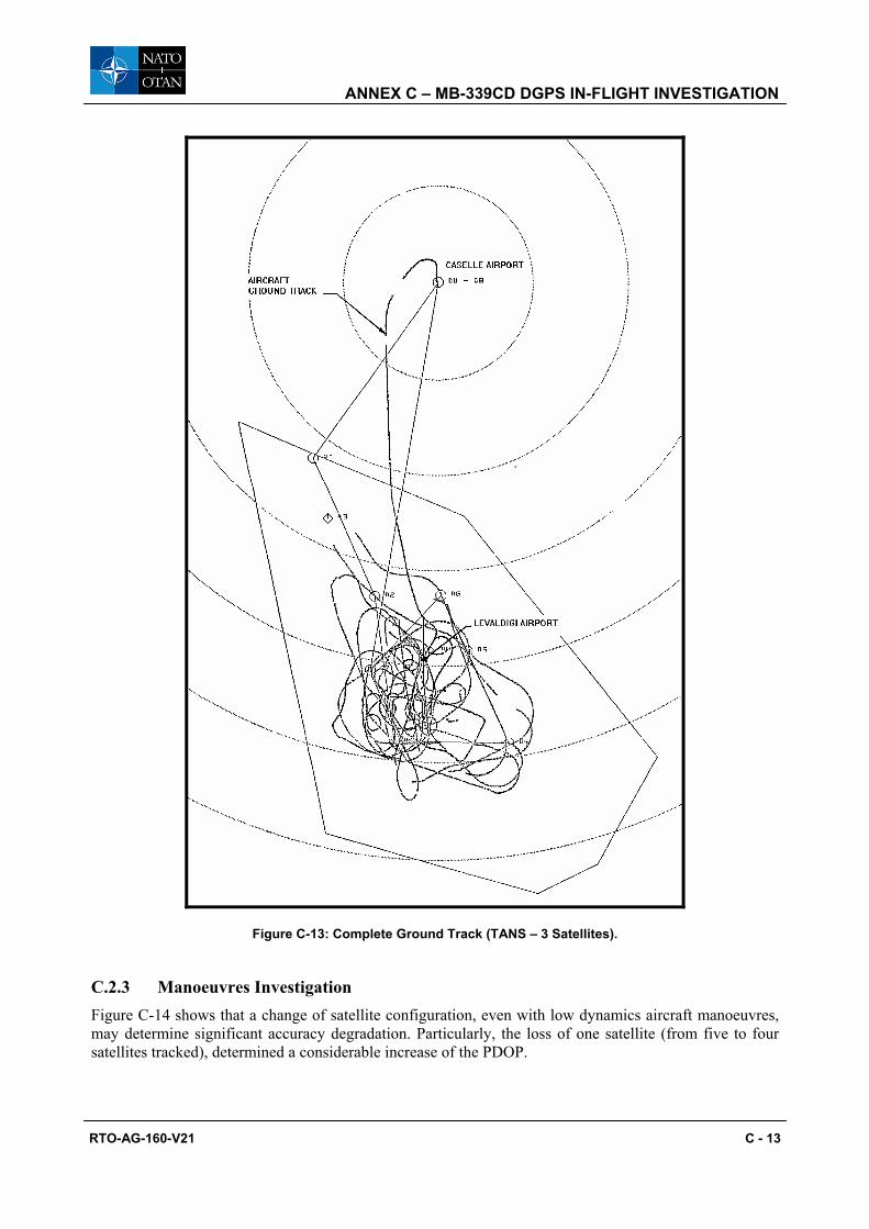
ANNEX C – MB-339CD DGPS IN-FLIGHT INVESTIGATION

RTO-AG-160-V21 C - 13

Figure C-13: Complete Ground Track (TANS – 3 Satellites).

C.2.3 Manoeuvres Investigation Figure C-14 shows that a change of satellite configuration, even with low dynamics aircraft manoeuvres, may determine significant accuracy degradation. Particularly, the loss of one satellite (from five to four satellites tracked), determined a considerable increase of the PDOP.

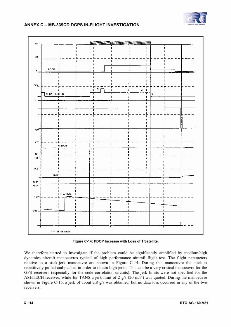
ANNEX C – MB-339CD DGPS IN-FLIGHT INVESTIGATION

C - 14 RTO-AG-160-V21

Figure C-14: PDOP Increase with Loss of 1 Satellite.

We therefore started to investigate if the problem could be significantly amplified by medium/high dynamics aircraft manoeuvres typical of high performance aircraft flight test. The flight parameters relative to a stick-jerk manoeuvre are shown in Figure C-14. During this manoeuvre the stick is repetitively pulled and pushed in order to obtain high jerks. This can be a very critical manoeuvre for the GPS receivers (especially for the code correlation circuits). The jerk limits were not specified for the ASHTECH receiver, while for TANS a jerk limit of 2 g/s (20 m/s3) was quoted. During the manoeuvre shown in Figure C-15, a jerk of about 2.8 g/s was obtained, but no data loss occurred in any of the two receivers.

ANNEX C – MB-339CD DGPS IN-FLIGHT INVESTIGATION

RTO-AG-160-V21 C - 15

Figure C-15: Stick-Jerk Manoeuvre.

The data shown in Figure C-16 were recorded during three pull-up manoeuvres at 4 g’s (typical in weapon-delivery trials). While during execution of the manoeuvres lock on to the satellites was kept (between four and three satellites tracked), at the end of each manoeuvre total signal losses occurred. The three manoeuvres were always preceded by straight-and-level flight (about 30 seconds) to allow optimal satellite tracking. Again, the reacquisition time after total signal losses was significantly longer for the TANS receiver than for the ASHTECH XII receiver.

Further tests were also performed with rapid-rolling horizontal manoeuvres (tonneau). In these cases, the lock to the satellites was efficiently maintained by both receivers, as long as the duration of the manoeuvres did not exceed a time about 5 seconds, which is considered adequate for the majority of flight tasks including rapid-rolling manoeuvres requirements. In general, the performances of the receivers during medium/high dynamics manoeuvres without turns were significantly better than the performances during turns with high bank angles (antenna masking).

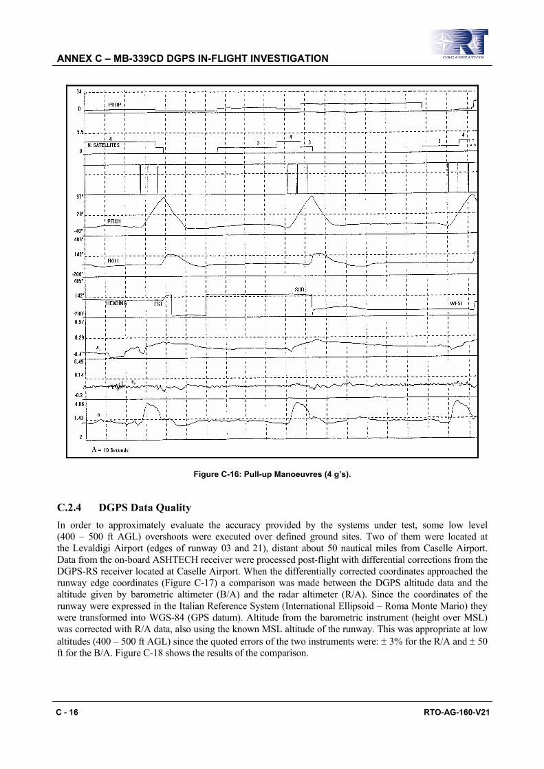
ANNEX C – MB-339CD DGPS IN-FLIGHT INVESTIGATION

C - 16 RTO-AG-160-V21

Figure C-16: Pull-up Manoeuvres (4 g’s).

C.2.4 DGPS Data Quality In order to approximately evaluate the accuracy provided by the systems under test, some low level (400 – 500 ft AGL) overshoots were executed over defined ground sites. Two of them were located at the Levaldigi Airport (edges of runway 03 and 21), distant about 50 nautical miles from Caselle Airport. Data from the on-board ASHTECH receiver were processed post-flight with differential corrections from the DGPS-RS receiver located at Caselle Airport. When the differentially corrected coordinates approached the runway edge coordinates (Figure C-17) a comparison was made between the DGPS altitude data and the altitude given by barometric altimeter (B/A) and the radar altimeter (R/A). Since the coordinates of the runway were expressed in the Italian Reference System (International Ellipsoid – Roma Monte Mario) they were transformed into WGS-84 (GPS datum). Altitude from the barometric instrument (height over MSL) was corrected with R/A data, also using the known MSL altitude of the runway. This was appropriate at low altitudes (400 – 500 ft AGL) since the quoted errors of the two instruments were: ± 3% for the R/A and ± 50 ft for the B/A. Figure C-18 shows the results of the comparison.

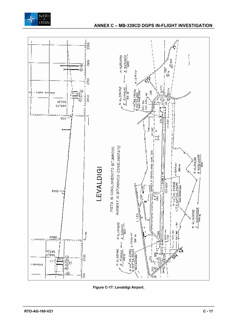
ANNEX C – MB-339CD DGPS IN-FLIGHT INVESTIGATION

RTO-AG-160-V21 C - 17

Figure C-17: Levaldigi Airport.

ANNEX C – MB-339CD DGPS IN-FLIGHT INVESTIGATION

C - 18 RTO-AG-160-V21

Figure C-18: Comparison of GPS and Altimeter Data.

C.3 DISCUSSION OF RESULTS

Analysing the data collected during the first DGPS flight test campaign conducted on the MB-339CD, it was concluded that the ASHTECH receiver was better suited than the TRIMBLE receiver for flight test applications. Particularly, the ASHTECH tracking and reacquisition strategy significantly reduced the time required for new position fixes after total GPS signal losses. Therefore, the ASHTECH XII data continuity during medium to high dynamics manoeuvres was significantly better than TANS. On average, the GPS data loss occurred in 25% of the total flight time for the ASHTECH receiver and in 35% of the time for the TANS. These results were obtained with similar settings of the threshold parameters for position computation.

The TANS receiver was able to provide a positioning solution even with only three satellites tracked, but in this case the accuracy degradation of the horizontal coordinates (especially the latitude) was significant.

The results of the data quality assessment carried out by comparing DGPS (ASHTECH) and barometric-radar altitude data were encouraging, but further investigation was required in order to evaluate the accuracy provided by the system.

RTO-AG-160-V21 D - 1

Annex D – TORNADO-IDS IN-FLIGHT INVESTIGATION

D.1 MASKING INVESTIGATION

In order to verify the masking conditions a special simulation software was implemented, called VIEWSAT, which modelled the aircraft shape and accepted input data such as the aircraft heading, pitch and bank angles in flight (from the FTI recorders), and positions of the satellites tracked during flight in terms of azimuth and elevation (Figure D-1).

Figure D-1: Satellite Visibility from Receiver Almanac Data.

The VIEWSAT software provided a visibility matrix (one dorsal antenna) for the defined flight conditions (Figure D-2), and required definition of a simplified aircraft model, as shown in Figure D-3.

Figure D-2: Example of Antenna Masking Matrix.

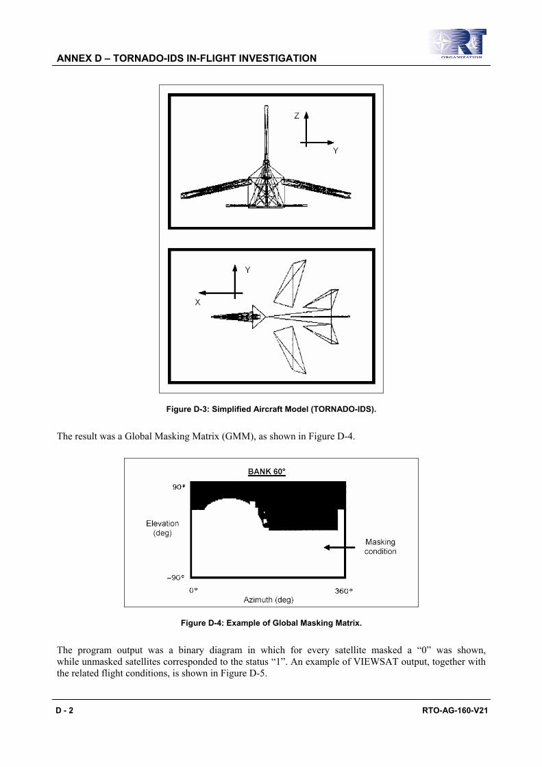
ANNEX D – TORNADO-IDS IN-FLIGHT INVESTIGATION

D - 2 RTO-AG-160-V21

Figure D-3: Simplified Aircraft Model (TORNADO-IDS).

The result was a Global Masking Matrix (GMM), as shown in Figure D-4.

Figure D-4: Example of Global Masking Matrix.

The program output was a binary diagram in which for every satellite masked a “0” was shown, while unmasked satellites corresponded to the status “1”. An example of VIEWSAT output, together with the related flight conditions, is shown in Figure D-5.

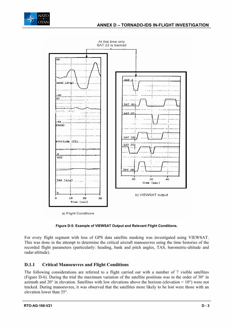
ANNEX D – TORNADO-IDS IN-FLIGHT INVESTIGATION

RTO-AG-160-V21 D - 3

Figure D-5: Example of VIEWSAT Output and Relevant Flight Conditions.

For every flight segment with loss of GPS data satellite masking was investigated using VIEWSAT. This was done in the attempt to determine the critical aircraft manoeuvres using the time histories of the recorded flight parameters (particularly: heading, bank and pitch angles, TAS, barometric-altitude and radar-altitude).

D.1.1 Critical Manoeuvres and Flight Conditions The following considerations are referred to a flight carried out with a number of 7 visible satellites (Figure D-6). During the trial the maximum variation of the satellite positions was in the order of 30° in azimuth and 20° in elevation. Satellites with low elevations above the horizon (elevation < 10°) were not tracked. During manoeuvres, it was observed that the satellites more likely to be lost were those with an elevation lower than 35°.

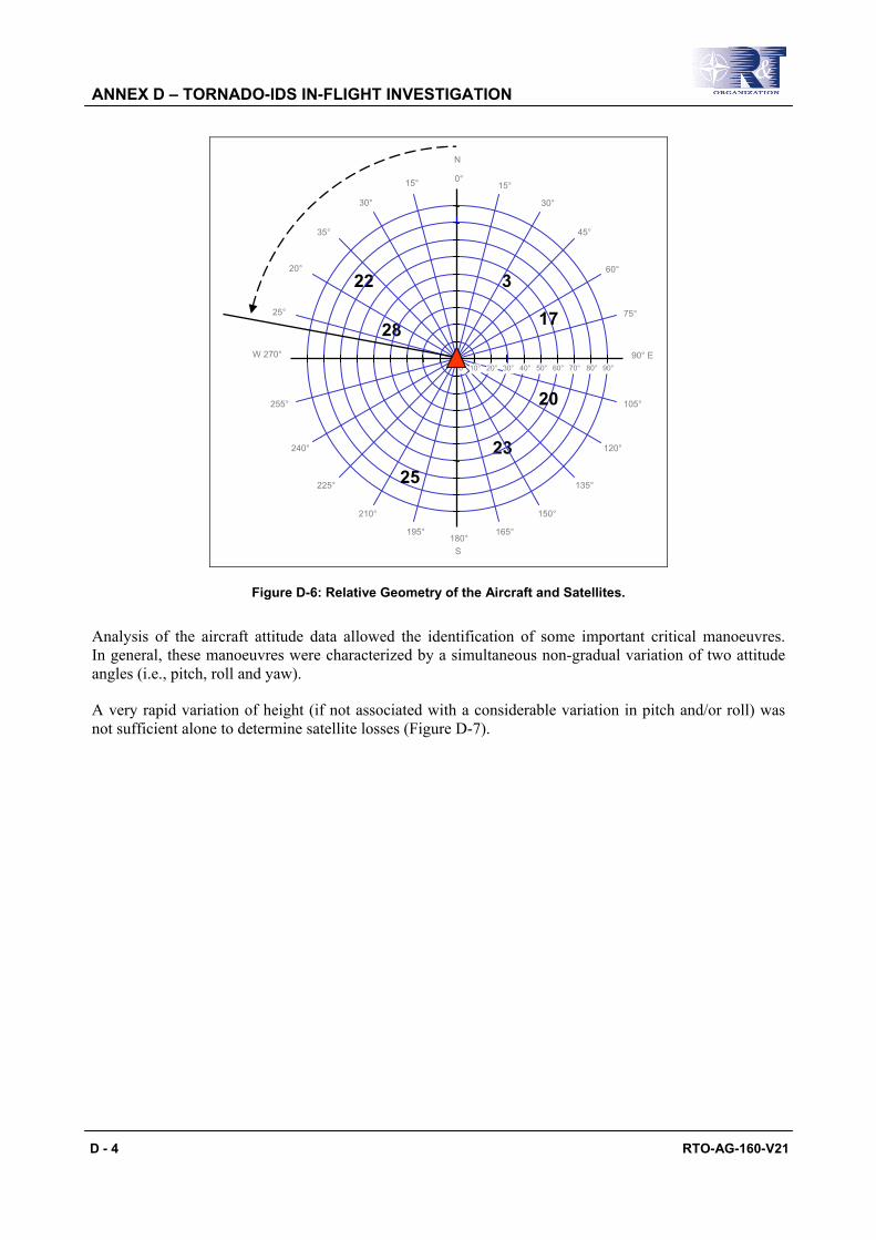
ANNEX D – TORNADO-IDS IN-FLIGHT INVESTIGATION

D - 4 RTO-AG-160-V21

23

22

28

3

90° E

75°

60°

45°

30°

15° 0° 15°

30°

35°

20°

25° W 270°

255°

240°

225°

210°

195°180°

165°

150°

135°

120°

105°

90° 80° 70° 60° 50° 40°30°20°10°0°

N

S

25

20

17

Figure D-6: Relative Geometry of the Aircraft and Satellites.

Analysis of the aircraft attitude data allowed the identification of some important critical manoeuvres. In general, these manoeuvres were characterized by a simultaneous non-gradual variation of two attitude angles (i.e., pitch, roll and yaw).

A very rapid variation of height (if not associated with a considerable variation in pitch and/or roll) was not sufficient alone to determine satellite losses (Figure D-7).

ANNEX D – TORNADO-IDS IN-FLIGHT INVESTIGATION

RTO-AG-160-V21 D - 5

(a) (b)

Figure D-7: Altitude Variations Without Satellite Signal Losses During Low Bank Manoeuvres (a) and in Vertical Flight (b).

A manoeuvre that was found to be very critical was the turn in the following conditions:

• Bank ≥ 50°; and

• Heading change > 90°.

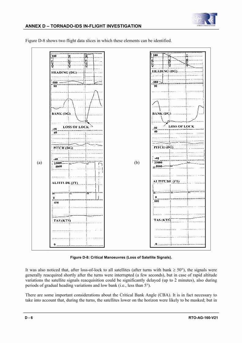
ANNEX D – TORNADO-IDS IN-FLIGHT INVESTIGATION

D - 6 RTO-AG-160-V21

Figure D-8 shows two flight data slices in which these elements can be identified.

(a) (b)

Figure D-8: Critical Manoeuvres (Loss of Satellite Signals).

It was also noticed that, after loss-of-lock to all satellites (after turns with bank ≥ 50°), the signals were generally reacquired shortly after the turns were interrupted (a few seconds), but in case of rapid altitude variations the satellite signals reacquisition could be significantly delayed (up to 2 minutes), also during periods of gradual heading variations and low bank (i.e., less than 5°).

There are some important considerations about the Critical Bank Angle (CBA). It is in fact necessary to take into account that, during the turns, the satellites lower on the horizon were likely to be masked; but in

ANNEX D – TORNADO-IDS IN-FLIGHT INVESTIGATION

RTO-AG-160-V21 D - 7

most cases the manoeuvre was critical only if the CBA was reached and maintained for a period of time exceeding about 5 seconds and with a large heading change (usually greater than 90°). In these cases, after 5 seconds, the number of satellites lost (n) was greater than (m – 4), being m the initial total number of satellites (Figure D-9).

22

28

3

90° E

75°

60°

45°

30°

15° 0° 15°

30°

35°

20°

25° W 270°

255°

240°

225°

210°

195°180°

165°

150°

135°

120°

105°

90 80 70 60 50403020100

N

S

CBA = 50°

Initial Heading

Critical Heading Change Final Heading Change

Masked Satellites Sector

2325

20

17

Figure D-9: Satellite Masking (SVs 17, 20, 23 and 25).

In many situations, however, the same manoeuvres did not determine the loss of lock to the satellites. The difference between the two cases (loss and no-loss) was represented by the fact that in the no-loss case the turns were following periods of stabilized flight (without significant heading, bank and height variations) longer than about 40 seconds. Figure D-10 shows a manoeuvre in which both the bank and the heading angles exceeded the critical values, but loss of GPS data did not occur. Similarly, also in the approach phase of a flight, a number of turns with high bank angles, progressively performed at lower altitudes, did not determine the signal loss (Figure D-11).

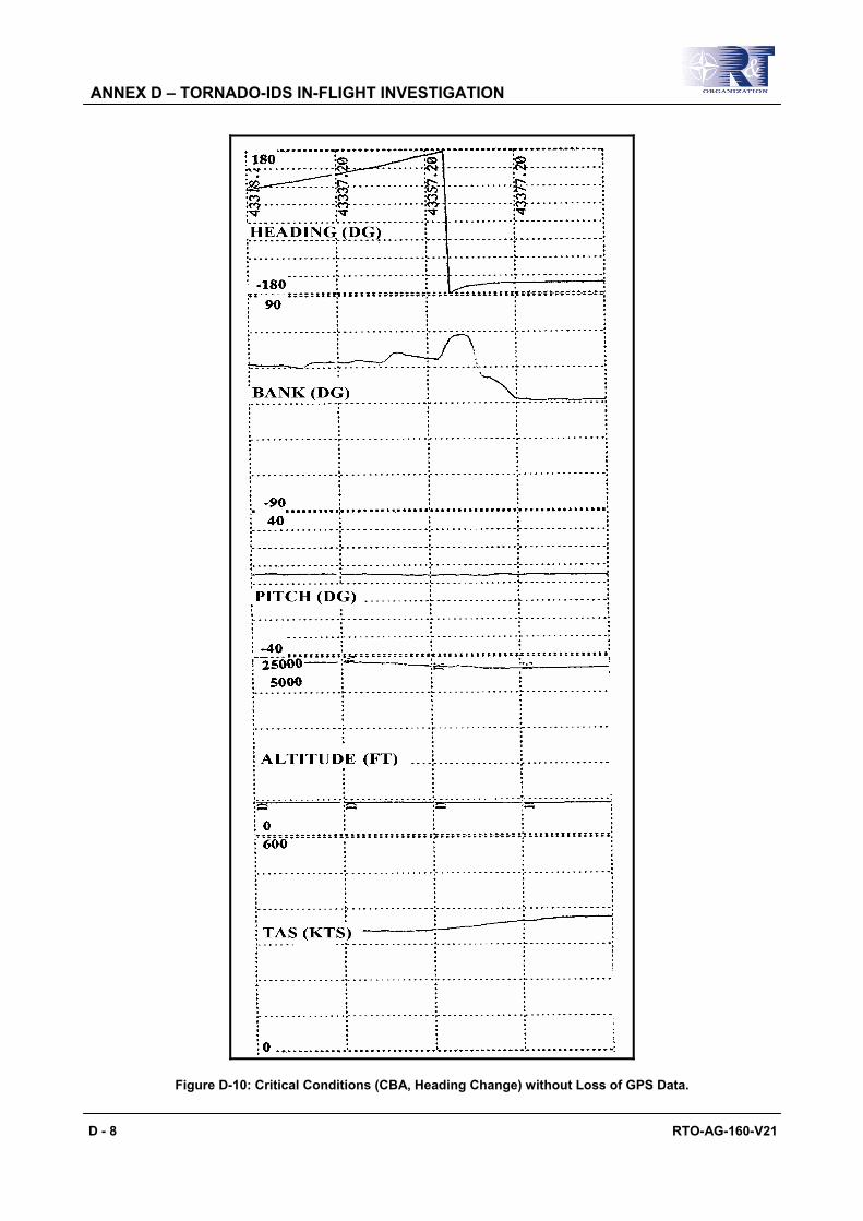
ANNEX D – TORNADO-IDS IN-FLIGHT INVESTIGATION

D - 8 RTO-AG-160-V21

Figure D-10: Critical Conditions (CBA, Heading Change) without Loss of GPS Data.

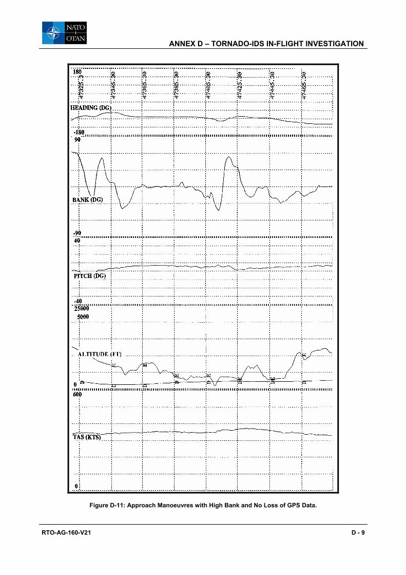
ANNEX D – TORNADO-IDS IN-FLIGHT INVESTIGATION

RTO-AG-160-V21 D - 9

Figure D-11: Approach Manoeuvres with High Bank and No Loss of GPS Data.

ANNEX D – TORNADO-IDS IN-FLIGHT INVESTIGATION

D - 10 RTO-AG-160-V21

Further analysis of the experimental data showed that the signal losses were maximised if the turns were started with an initial aircraft heading in the sectors from north-east to south-east in case of left turns and from south-west to north-west in case of right turns. In order to assist in the investigation of this evidence, we started examining the characteristics of typical “sky-plots” (i.e., satellites azimuth and elevations observed from certain locations on the hearth surface and for a certain period of time) that can be obtained at our latitudes. Figure D-12 shows a sky-plot relative to the city of Rome (date: 25th June 2005; coordinates: North 41° 52’, East 12° 37’, h = 0; duration: 24 hours).

Right Turn Left Turn

45° 315°

135° 225°

Figure D-12: GPS Sky-Plot.

It is evident that in the northern hemisphere/mid-latitudes the majority of satellites are available in the azimuth range 45° ÷ 315°, and that a left turn of an aircraft with an initial heading in the range 45° ÷ 135° (i.e., north-east ÷ south-east) would be prone to GPS data losses, due to the reduced number of satellites available in the direction of the turn. Similar considerations apply for the right turns performed with an initial heading in the range 225° ÷ 315° (i.e., south-west ÷ north-west).

D.1.2 Reacquisition Time On average the ASHTECH receiver was able to give a new position solution within about 20 seconds from restoration of the line-of-sight conditions to the satellites. Therefore, it was generally sufficient to maintain a low bank angle for about 20 seconds in order to obtain a new solution. However, if the height was kept constant the time required was reduced to about 10 seconds. This can be seen comparing the diagrams in Figure D-8(a) with the corresponding VIEWSAT diagram shown in Figure D-13.

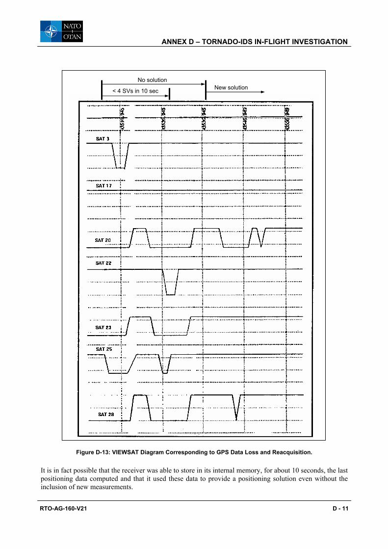
ANNEX D – TORNADO-IDS IN-FLIGHT INVESTIGATION

RTO-AG-160-V21 D - 11

Figure D-13: VIEWSAT Diagram Corresponding to GPS Data Loss and Reacquisition.

It is in fact possible that the receiver was able to store in its internal memory, for about 10 seconds, the last positioning data computed and that it used these data to provide a positioning solution even without the inclusion of new measurements.

New solution No solution

< 4 SVs in 10 sec

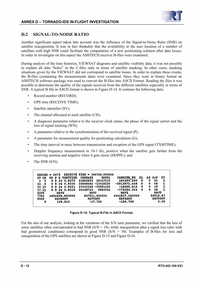
ANNEX D – TORNADO-IDS IN-FLIGHT INVESTIGATION

D - 12 RTO-AG-160-V21

D.2 SIGNAL-TO-NOISE RATIO

Another significant aspect taken into account was the influence of the Signal-to-Noise Ratio (SNR) on satellite reacquisition. It was in fact thinkable that the availability at the user location of a number of satellites with high SNR could facilitate the computation of a new positioning solution after data losses. In order to investigate on this aspect the ASHTECH receiver B-files were examined.

During analysis of the time histories, VIEWSAT diagrams and satellite visibility data, it was not possible to explain all data “holes” in the C-files only in terms of satellite masking. In other cases, masking situations given by the VIEWSAT did not correspond to satellite losses. In order to explain these events, the B-files (containing the measurements data) were examined. Since they were in binary format an ASHTECH software package was used to convert the B-files into ASCII Format. Reading the files it was possible to determine the quality of the signals received from the different satellites especially in terms of SNR. A typical B-file in ASCII format is shown in Figure D-14. It contains the following data:

• Record number (RECORD);

• GPS time (RECEIVE TIME);

• Satellite identifier (SV);

• The channel allocated to each satellite (CH);

• A diagnosis parameter relative to the receiver clock status, the phase of the signal carrier and the loss of signal tracking (WN);

• A parameter relative to the synchronisation of the received signal (P);

• A parameter for measurement quality for positioning calculation (G);

• The time interval in msec between transmission and reception of the GPS signal (TXMTIME);

• Doppler frequency measurement in 10-1 Hz, positive when the satellite gets farther from the receiving antenna and negative when it gets closer (DOPPL); and

• The SNR (S/N).

Figure D-14: Typical B-File in ASCII Format.

For the aim of our analysis, looking at the variations of the S/N ratio parameter, we verified that the loss of some satellites often corresponded to bad SNR (S/N < 10), while reacquisition after a signal loss (also with bad geometrical conditions) correspond to good SNR (S/N > 30). Examples of B-files for loss and reacquisition of the GPS satellites are shown in Figure D-15 and Figure D-16.

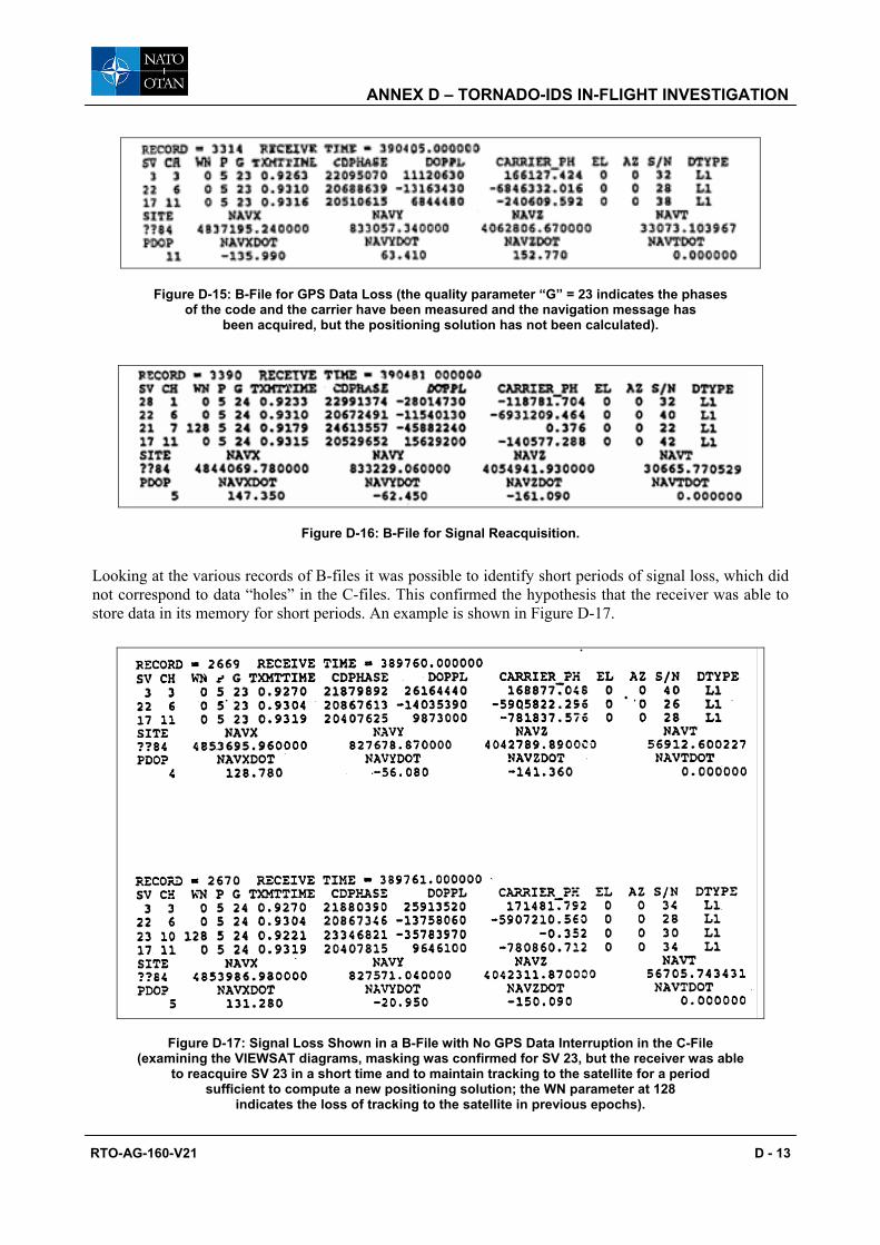
ANNEX D – TORNADO-IDS IN-FLIGHT INVESTIGATION

RTO-AG-160-V21 D - 13

Figure D-15: B-File for GPS Data Loss (the quality parameter “G” = 23 indicates the phases of the code and the carrier have been measured and the navigation message has

been acquired, but the positioning solution has not been calculated).

Figure D-16: B-File for Signal Reacquisition.

Looking at the various records of B-files it was possible to identify short periods of signal loss, which did not correspond to data “holes” in the C-files. This confirmed the hypothesis that the receiver was able to store data in its memory for short periods. An example is shown in Figure D-17.

Figure D-17: Signal Loss Shown in a B-File with No GPS Data Interruption in the C-File (examining the VIEWSAT diagrams, masking was confirmed for SV 23, but the receiver was able

to reacquire SV 23 in a short time and to maintain tracking to the satellite for a period sufficient to compute a new positioning solution; the WN parameter at 128

indicates the loss of tracking to the satellite in previous epochs).

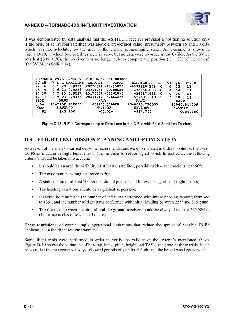
ANNEX D – TORNADO-IDS IN-FLIGHT INVESTIGATION

D - 14 RTO-AG-160-V21

It was demonstrated by data analysis that the ASHTECH receiver provided a positioning solution only if the SNR of at list four satellites was above a pre-defined value (presumably between 15 and 30 dB), which was not selectable by the user at the ground programming stage. An example is shown in Figure D-18, in which four satellites were in view, but no data were recorded in the C-files. As the SV 28 was lost (S/N < 30), the receiver was no longer able to compute the position (G = 23) of the aircraft (the SV 24 has SNR = 14).

Figure D-18: B-File Corresponding to Data Loss in the C-File with Four Satellites Tracked.

D.3 FLIGHT TEST MISSION PLANNING AND OPTIMISATION

As a result of the analysis carried out some recommendations were formulated in order to optimise the use of DGPS as a datum in flight test missions (i.e., in order to reduce signal loses). In particular, the following criteria’s should be taken into account:

• It should be assured the visibility of at least 6 satellites, possibly with 4 at elevations near 50°;

• The maximum bank angle allowed is 50°;

• A stabilisation of at least 20 seconds should precede and follow the significant flight phases;

• The heading variations should be as gradual as possible;

• It should be minimised the number of left turns performed with initial heading ranging from 45° to 135°, and the number of right turns performed with initial heading between 225° and 315°; and

• The distance between the aircraft and the ground receiver should be always less than 200 NM to obtain accuracies of less than 5 metres.

These restrictions, of course, imply operational limitations that reduce the spread of possible DGPS applications in the flight test environment.

Some flight trials were performed in order to verify the validity of the criteria’s mentioned above. Figure D-19 shows the variations of heading, bank, pitch, height and TAS during one of these trials. It can be seen that the manoeuvres always followed periods of stabilised flight and the height was kept constant.

ANNEX D – TORNADO-IDS IN-FLIGHT INVESTIGATION

RTO-AG-160-V21 D - 15

Figure D-19: Optimised Manoeuvres for DGPS Data Gathering.

The visible constellation during the flight sortie included a total of eight satellites, with at list four having an average elevation grater than 50° and two with an elevation always greater than 30°. The trajectory diagram shown in Figure D-20 is completely free from signal losses.

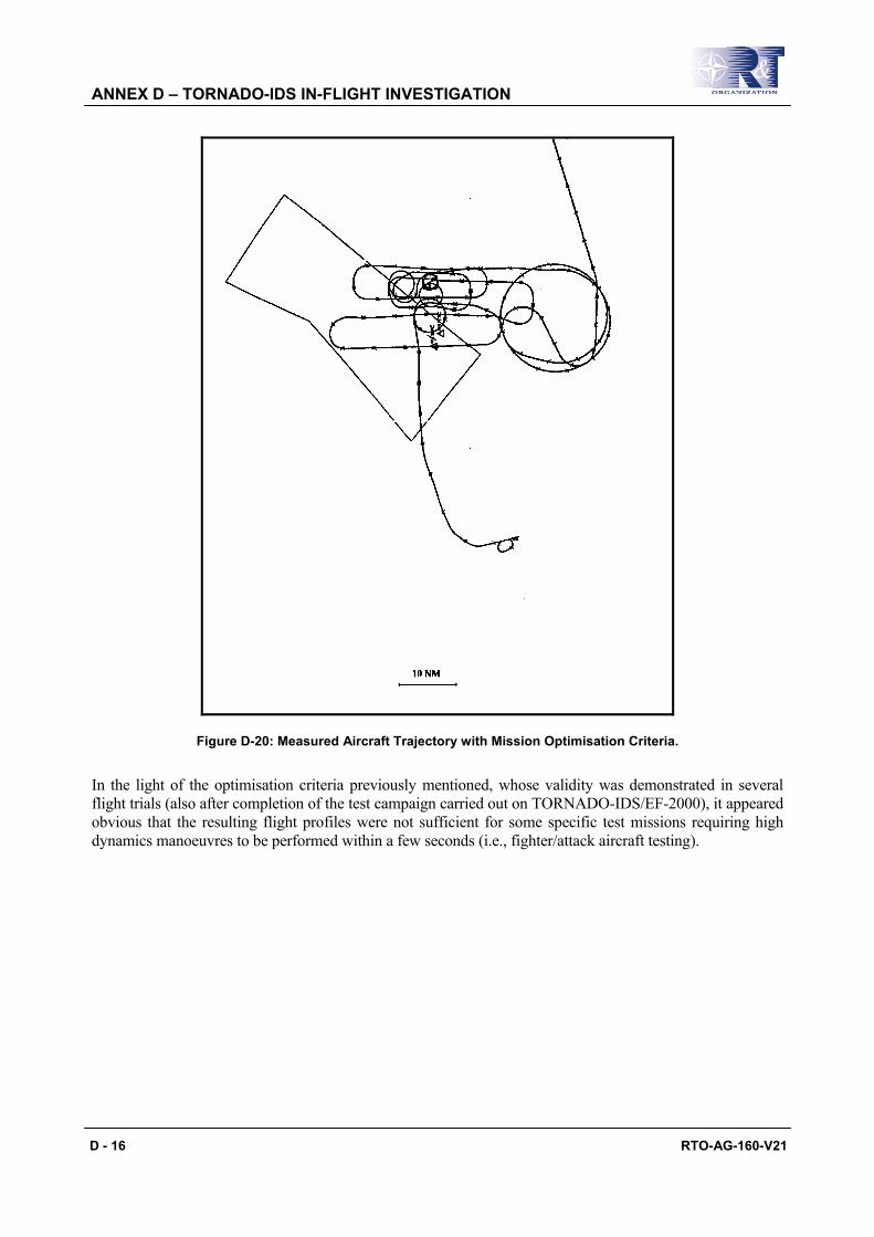
ANNEX D – TORNADO-IDS IN-FLIGHT INVESTIGATION

D - 16 RTO-AG-160-V21

Figure D-20: Measured Aircraft Trajectory with Mission Optimisation Criteria.

In the light of the optimisation criteria previously mentioned, whose validity was demonstrated in several flight trials (also after completion of the test campaign carried out on TORNADO-IDS/EF-2000), it appeared obvious that the resulting flight profiles were not sufficient for some specific test missions requiring high dynamics manoeuvres to be performed within a few seconds (i.e., fighter/attack aircraft testing).

RTO-AG-160-V21 E - 1

Annex E – DGPS/INS INTEGRATION

E.1 INTRODUCTION

The benefits of integrating GPS (or DGPS) with an INS are significant and diverse. Basically, each system has important shortcomings. Used in concert through some adequate algorithm, the integrated system solves the majority of these problems. All of the GPS techniques (either stand-alone or differential) suffer from some shortcomings. The most important are:

• The data rate of a GPS receiver is too low and the latency is too large to satisfy the requirements for high performance aircraft trajectory analysis, in particular with respect to the synchronisation with external events. In addition, there might be a requirement for high-rate and small latency trajectory data to provide real-time guidance information to the pilot (e.g., during fly-over-noise measurements). With the need to process radio frequency signals and the complex processing required to formulate a position or velocity solution [1], GPS data rates are usually at 1 Hz, or at best 10 Hz (an update rate of at least 20 Hz is required for real-time applications);

• High DGPS accuracy is limited by the distance between the Reference Station and the user because of the problem of ionosphere in integer ambiguity resolution on-the-fly [2];

• Selective Availability (SA) degrades differential GPS positioning accuracy over long distances;

• Influences of high accelerations on the GPS receiver clock, the code tracking loop and carrier phase loop may become significant; and

• Signal loss-of-lock and ‘cycle slips’ may occur very frequently due to aircraft manoeuvres or other causes.

There is little one can do to ensure the continuity of the signal propagation from the satellite to the receiver during high dynamic manoeuvres. Due to shadowing of the GPS antenna the receiver will loose track to several and in many cases to all satellites (see Chapter 8 and 9).

Stand-alone INS has its shortcomings as well. The INS is subject to an ever growing drift in position accuracy caused by various instrument error sources that cannot be eliminated in manufacturing, assembly, calibration or initial system alignment [1]. Furthermore, high quality inertial systems (i.e., platform systems) tend to be complex and expensive devices with significant risk of component failure.

The integration of (D)GPS and INS measurements might solve most of the above mentioned shortcomings: the basic update rate of an INS is 50 samples per second or higher and an INS is a totally self-contained system. The combination of INS and (D)GPS will therefore provide the required update rate, data continuity and integrity. The other advantages of an INS: low short term drift and low noise, are combined with the advantages of (D)GPS: high position accuracy and no long term drift. Therefore, in the case of DGPS/INS integration, the real-time demands on the telemetry data link are not very high because INS errors show a long term drift only and thus do not need to be updated frequently [3].

E.2 DGPS/INS INTEGRATION

Technical considerations for integration of DGPS and INS include the choice of system architecture, the integration algorithm (mostly Kalman Filter), and the characterisation and modelling of the measurements produced by the two sensors. Traditionally, GPS has been used to update the position of the INS (in other words, to control the drift behaviour of the INS). When looking to the high accuracy potential of DGPS, it is obvious to go the other way around, namely to get the positioning information primarily from GPS. Thus, the INS is now becoming the secondary sensor enabling higher interpolation in

ANNEX E – DGPS/INS INTEGRATION

E - 2 RTO-AG-160-V21

GPS positioning updates, providing the attitude information, damping short periodic influences in GPS, and assisting in cycle slip detection and on-the-fly ambiguity resolution algorithms [4]. Clearly, both types of observations enter the Kalman filter, and only the different weighting of the data decides which sensor mainly contributes to the integrated result.

In principle, integration of DGPS with the INS can be done in levels analogously to the DGPS methods, using:

• DGPS differential pseudorange corrections [5];

• DGPS carrier phase-smoothed pseudorange corrections [5]; and

• DGPS carrier phase corrections [6].

These are also the data which can be transmitted by telemetry from the reference station to the user when following the RTCM standardised messages. For a real-time fully integrated DGPS/INS application it is clear that also the appropriate raw data, pseudoranges and carrier phases have to be transmitted, perhaps in a compressed form in order to minimise the telemetry load (e.g., in the form of pseudorange and carrier phase corrections).

Integration of INS with DGPS can be carried out in many different ways depending on the application (i.e., online/off-line evaluation, accuracy requirements). In the following paragraphs some information are given about integration algorithms for both real-time and post-processing systems.

E.3 INTEGRATION ALGORITHMS

Various options exist for the integration algorithm. In general, two main categories can be identified depending on the application: post-processing and real-time algorithms. The complexity of the algorithm is obviously related to both system accuracy requirements and computer load capacity. While for many applications a post-processing solution is acceptable, this is not useful for both navigation and online evaluation during a flight test. The state-of-the-art integration algorithm is the Kalman Filter (KF). In general terms, a KF is a recurrent, optimal estimator used in many engineering applications whenever the estimation of the state of a dynamic system is required. A KF can be used to estimate the errors which affect the solution computed in an INS or in a (D)GPS, as well as in the combination of both navigation sensors. An analytic description of Kalman filters and other integration algorithms can be found in the literature [7, 8]. In the following paragraphs some information are given about DGPS/INS Kalman filter implementations.

E.3.1 Kalman Filters A number of implementations are possible for the (D)GPS/INS Kalman Filter. Matrix formulation methods of various types have been developed to improve numerical stability and accuracy (e.g., square root and stabilised formulations), to minimise the computational complexity by taking advantage of the diagonal characteristics of the covariance matrix (U-D factorisation formulation), and to estimate state when the state functions are non-linear (extended Kalman filter).

In general, the KF algorithm is optimal under three limiting conditions: the system model is linear, the noise is white and Gaussian with known autocorrelation function and the initial state is known. None of them are strictly verified in practice. Moreover, the computing burden grows considerably with increasing number of states modelled. Artificial Neural Networks (ANN) could be used to relax one or more of the conditions under which the KF is optimal and/or reduce the computing requirements of the KF. While the total replacement of KF with ANN filters lead to difficult design and unreliable integration functions, a hybrid network in which the ANN is used to learn the corrections to be applied to the state

ANNEX E – DGPS/INS INTEGRATION

RTO-AG-160-V21 E - 3

prediction performed by a rule-based module, appears as the best candidate for future navigation sensor integration.

In the following paragraphs some examples are given of algorithms adopting a KF (or part of it) for integration of (D)GPS and INS measurements.

E.3.1.1 Rauch-Tung-Striebel-Algorithm

Post-processing integration of (D)GPS and INS measurements can be carried out by means of the Rauch-Tung-Striebel algorithm, which consists of a Kalman filter and a backward smoother. The forward filter can take into account previous measurements only. The smoothed estimate utilises all measurements. It is obvious that the smoothed positions are always at least as accurate as the forward filtered positions. In most cases, however, the smoothed positions are considerably more accurate than the filtered ones. It is evident that backward smoothing can only be done off-line. The filter estimates the state vector together with the error covariance matrix. The state vector contains the error components of the inertial navigation system. The smoothed trajectories and also accurate velocities are obtained by adding the state vector to the measurements delivered by the INS. The equations of the Rauch-Tung-Striebel algorithm can be found in reference [7]. With this system, an integration between (D)GPS and INS is possible and the high frequency movements of the aircraft are not smoothed out. Both positions and velocities can be obtained with a high degree of accuracy and are nearly continuously available. This is also true when the time interval between the measurements is relatively long (e.g., 1 min). There is a need to carry out a great amount of calculations and to store much data for the backward filter, but with modern computers this is not a major problem.

E.3.1.2 U-D Factorised Kalman Filter

The filtering algorithm most commonly implemented in real-time systems is the Bierman’s U-D Factorised Kalman Filter. This algorithm avoids the explicit and computation of the estimation error covariance matrix Pt by propagating in terms of its factors U and D:

P UDUtT= (E.1)

where U is a unit upper triangular matrix and D is a diagonal matrix. The U and D factors are calculated by the modified weighted Gram-Schmitt (MWGS) algorithm [9]. The U-D algorithm is efficient and provides significant advantages in numerical stability and precision. Specifically, the factorisation of Pt provides an effective doubling in computer word length in covariance-related calculations, and avoids filter divergence problems which can arise in more conventional filter mechanisations [7].

E.3.1.3 Artificial Neural Networks and Hybrid Networks

Although Artificial Neural Networks technology has not been fully investigated for application to integrated air navigation systems, the suitability of such technology to replace or enhance the performance of the Kalman Filter has been proven in related areas [10, 11]. However, the development of an integration algorithm completely based on neural technology (e.g., Hopfield Networks) appears impracticable at the moment. Furthermore, this solution is even more demanding than the Kalman Filter in terms of computing requirements [12]. Techniques for “On-line Training” would allow for real-time adaptation to the specific operating conditions, but further research is required in this field.

Hybrid Networks emerge as the best candidate for future applications. In an hybrid architecture an ANN is used in combination with a rule-based system (i.e., a complete Kalman Filter or part of it), in order to achieve the required adaptivity and improve the availability of the overall system. A hybrid network provides performances comparable with the Kalman Filter, but with improved adaptivity to non-linearities

ANNEX E – DGPS/INS INTEGRATION

E - 4 RTO-AG-160-V21

and unpredicted changes in system/environment parameters. Compared with the Kalman Filter, the hybrid architecture features the high parallelism of the neural structure allowing for faster operation and higher robustness to hardware failures. The use of ANN to correct the state variables prediction operated by the rule-based module avoids computing the Kalman gain, thus considerably reducing the computing burden. Stability may be guaranteed if the output of the network is in the form of correction to a nominal gain matrix that provides a stable solution for all system parameters. The implementation of such a filter, however, would be sensitive to network topology and training strategy. An adequate testing activity would therefore be required.

E.4 INTEGRATION ARCHITECTURES

Combining (D)GPS and INS, different depths of integration can be realised. The level of integration and the particular mechanisation of the Kalman filter are dependent on:

• The task of the integration;

• The accuracy limits;

• The robustness and the stand alone capacity of each subsystem;

• The INS sensor concept (platform/strapdown); and

• The computer time capacity.

For these tasks, the basic concepts of system integration can be divided into the following topics:

• Open loop (D)GPS aided INS (OLDI);

• Closed loop (D)GPS aided INS (CLDI); and

• Fully integrated (D)GPS/INS (FIDI).

In the following paragraphs only a brief description of the various architectures is given. Further information can be found in the references [1, 13, 14].

E.4.1 Open Loop Systems The simplest way to combine (D)GPS and INS is a reset-only mechanisation in which (D)GPS is used to periodically reset the INS solution. In this open-loop strategy the INS is not re-calibrated by (D)GPS data, so the underlying error sources in the INS still drive its navigation errors as soon as (D)GPS resets are interrupted. However, for short (D)GPS interruptions or for high quality INS, the error growth may be small enough to meet mission requirements. This is why platform inertial systems have to be used with OLDI systems operating in a high dynamic environment (e.g., military aircraft). The advantage of the open loop implementation is that, in case of inaccurate measurements, just the Kalman filter is influenced and not the inertial system calculation itself. As the sensors of a platform system are separated from the body of the aircraft by gimbals, they are operating normally at their reference point zero. The attitude angles are measured by the angles of the gimbals. The Kalman filter can run internal or external to the INS, but the errors of the inertial system have to be carefully modelled.

E.4.2 Closed Loop Systems The main advantage of (D)GPS aiding the INS in a closed-loop mechanisation is that the INS is continuously calibrated by the Kalman Filter, using the (D)GPS data. Therefore strapdown sensors can be used in a CLDI implementation.

ANNEX E – DGPS/INS INTEGRATION

RTO-AG-160-V21 E - 5

In contrary to platform systems, sensors of strapdown INS are not uncoupled from the aircraft body. They are operating in a dynamically more disturbed environment as there are vibrations, angular accelerations, angular oscillations which result in an additional negative influence to the system performance. In addition sensors are not operating at a reference point zero. Therefore the errors of the system will increase very rapidly and problems of numerical inaccuracy in an open loop implementation may soon increase. This is why it is advantageous to loop back the estimated sensor errors to the strapdown calculations in order to compensate for the actual system errors. Consequently, the errors of the INS will be kept low and linear error models can be used. When (D)GPS data is lost due to dynamics or satellite shadowing, the INS can continue the overall solution, but now as a highly precise unit by virtue of its recent calibration. However, this system implementation can be unstable.

E.4.3 Fully Integrated Systems The system integration of best accuracy will be of course the full integration of both systems which requires a Kalman filter implementation at a raw/uncorrelated measurements level.

As the Kalman filter theory asks for uncorrelated measurements [7], it is optimal to use either the raw GPS measurements (i.e., the range and phase measurements to at least four satellites, the ephemeris to calculate the satellite positions and the parameters to correct for the ionospheric and troposphere errors), or (D)GPS position (and velocity) data uncorrelated between update intervals [15]. In the first case, the receiver clock errors (time offset and frequency) can be estimated as a part of the filter model.

This approach has very complex measurement equations, but requires only one Kalman Filter mechanisation. Moreover, its filtering can be most optimal since both (D)GPS errors and INS errors can be included without the instability problems typical of cascade Kalman Filters.

E.4.4 OLDI/CLDI and FIDI Comparison The most important distinction to be made is between cascaded and non-cascaded approaches, which correspond, as mentioned before, to aided (OLDI and CLDI) or fully integrated (FIDI) architectures respectively. In the cascaded case two filters generally play the role. The first filter is a GPS filter which produces outputs (i.e., position and velocity) which are correlated between measurement times. This output is then used as input for the second filter which is the INS Kalman filter. As time correlation of this measurement input does not comply with the assumptions underlying the standard Kalman filter [7], it must be accounted for in the right way [16]. This will complicate the Kalman filter design (i.e., the potential instability of cascaded filters makes the design of the integration Kalman filter a very cautious task). However, from a hardware implementation point of view aided INS (in both OLDI and CLDI configurations) results in the simplest solution. In the non-cascaded case there is just a single Kalman filter generally based on an INS error model supplemented by a GPS error model. The GPS measurements, uncorrelated between measurement times, are differenced with the raw INS data to give measurements of the INS errors, also uncorrelated between measurements times.

E.5 REFERENCES

[1] Siouris, G.M. (1993). “Aerospace Avionics Systems”. Academic Press, San Diego, California (USA).

[2] Hein, G.W. and Ertel, M.M. (1993). “High-precision Aircraft Navigation using DGPS/INS integration”. Institute of Astronomical and Physical Geodesy (IAPG). University FAF Munich, Neubiberg (Germany).

[3] Kleusberg, A. (1986). “Kinematic Relative Positioning Using GPS Code and Carrier Beat Phase Observations”. Marine Geodesy.

ANNEX E – DGPS/INS INTEGRATION

E - 6 RTO-AG-160-V21

[4] Hein, G.W., Baustert, G. and Landau, H. (1989). “High-Precision Kinematic GPS Differential Positioning and Integration of GPS with a Ring Laser Strapdown Inertial System”. Institute of Astronomical and Physical Geodesy (IAPG). University FAF Munich, Neubiberg (Germany).

[5] RTCM Special Committee No. 104. (1994). “RTCM Recommended Standards for Differential NAVSTAR GPS Service”. Radio Technical Committee for Maritime Services. Paper 194-93/SC104-STD. Washington DC (USA).

[6] Gloecker, F., Van Dierendonck, A.J. and Hatch, R. (1992). “Proposed Revisions to RTCM SC-104, Recommended Standards for Differential NAVSTAR GPS Service for Carrier Phase Applications”. Proceedings of ION-92, 5th International Technical Meeting of the Satellite Division of the Institute of Navigation. Albuquerque (USA).

[7] Gelb, A. (1992). “Applied Optimal Estimation”. The MIT Press. Cambridge (Massachusetts), and London (England).

[8] Waltz, E. and Linas, J. (1994). “Multisensor Data Fusion”. Artech House. London, New York. Second Edition, pp. 159-211.

[9] Bierman, G.J. (1977). “Factorisation Methods for Discrete Sequential Estimation”. Academic Press. New York.

[10] Dumville, M. and Tsakiri, M. (1994). “An Adaptive Filter for Land Navigation Using Neural Computing”. Proceedings of ION GPS-94.

[11] Currie, M.G. (1992). “An Optimized Filter Architecture Incorporating a Neural Network”. International Conference on Neural Networks. Baltimora (USA).

[12] Lo Conte, R. (1996). “Artificial Neural Networks to Enhance or Replace the Kalman Filter in INS”. N° 28 GD Aerosystems Course Personal Project. Air Warfare Centre, Operational Doctrine and Training. Royal Air Force Cranwell.

[13] Joint Program Office (JPO). (1991). “NAVSTAR GPS User Equipment, Introduction”. Public Release Version. US Air Force Space Systems Division, NAVSTAR-GPS Joint Program Office (JPO). Los Angeles AFB, California (USA).

[14] Jacob, T. and Schanzer, G. (1989). “Integrated Flight Guidance System Using Differential GPS for Landing Approach Guidance”. AGARD-CP-455. NATO Advisory Group for Aerospace Research and Development. Neuilly-sur-Seine (France).

[15] Van de Leijgraaf, R., Breeman, J., Moek, G. and Van Leeuwen, S.S. (1993). “A Position Reference System for Fokker 70”. NLR Technical Publication TP 93084L.

[16] Napier, M. (1989). “The Integration of Satellite and Inertial Positioning Systems”. Proceedings of the Symposium NAV-89. The Royal Institute of Navigation. London.

RTO-AG-160-V21 F - 1

Annex F – AGARD and RTO Flight Test Instrumentation and Flight Test Techniques Series

1. Volumes in the AGARD and RTO Flight Test Instrumentation Series, AGARDograph 160

Volume Title Publication Number Date

1. Basic Principles of Flight Test Instrumentation Engineering (Issue 2) Issue 1: Edited by A. Pool and D. Bosman 1974 Issue 2: Edited by R. Borek and A. Pool 1994

2. In-Flight Temperature Measurements 1973 by F. Trenkle and M. Reinhardt

3. The Measurements of Fuel Flow 1972 by J.T. France

4. The Measurements of Engine Rotation Speed 1973 by M. Vedrunes

5. Magnetic Recording of Flight Test Data 1974 by G.E. Bennett

6. Open and Closed Loop Accelerometers 1974 by I. McLaren

7. Strain Gauge Measurements on Aircraft 1976 by E. Kottkamp, H. Wilhelm and D. Kohl

8. Linear and Angular Position Measurement of Aircraft Components 1977 by J.C. van der Linden and H.A. Mensink

9. Aeroelastic Flight Test Techniques and Instrumentation 1979 by J.W.G. van Nunen and G. Piazzoli

10. Helicopter Flight Test Instrumentation 1980 by K.R. Ferrell

11. Pressure and Flow Measurement 1980 by W. Wuest

12. Aircraft Flight Test Data Processing – A Review of the State of the Art 1980 by L.J. Smith and N.O. Matthews

13. Practical Aspects of Instrumentation System Installation 1981 by R.W. Borek

14. The Analysis of Random Data 1981 by D.A. Williams

15. Gyroscopic Instruments and Their Application to Flight Testing 1982 by B. Stieler and H. Winter

16. Trajectory Measurements for Take-off and Landing Test and Other Short-Range 1985 Applications by P. de Benque D’Agut, H. Riebeek and A. Pool

ANNEX F – AGARD AND RTO FLIGHT TEST INSTRUMENTATION AND FLIGHT TEST TECHNIQUES SERIES

F - 2 RTO-AG-160-V21

17. Analogue Signal Conditioning for Flight Test Instrumentation 1986 by D.W. Veatch and R.K. Bogue

18. Microprocessor Applications in Airborne Flight Test Instrumentation 1987 by M.J. Prickett

19. Digital Signal Conditioning for Flight Test 1991 by G.A. Bever

20. Optical Air Flow Measurements in Flight 2003 by R.K. Bogue and H.W. Jentink

21. Differential Global Positioning System (DGPS) for Flight Testing 2008 by R. Sabitini and G.B. Palmerini

ANNEX F – AGARD AND RTO FLIGHT TEST INSTRUMENTATION AND FLIGHT TEST TECHNIQUES SERIES

RTO-AG-160-V21 F - 3

2. Volumes in the AGARD and RTO Flight Test Techniques Series

Volume Title Publication Number Date

AG237 Guide to In-Flight Thrust Measurement of Turbojets and Fan Engines by the MIDAP 1979 Study Group (UK)

The remaining volumes are published as a sequence of Volume Numbers of AGARDograph 300.

1. Calibration of Air-Data Systems and Flow Direction Sensors 1988 by J.A. Lawford and K.R. Nippress

2. Identification of Dynamic Systems 1988 by R.E. Maine and K.W. Iliff

3. Identification of Dynamic Systems – Applications to Aircraft Part 1: The Output Error Approach 1986 by R.E. Maine and K.W. Iliff Part 2: Nonlinear Analysis and Manoeuvre Design 1994 by J.A. Mulder, J.K. Sridhar and J.H. Breeman

4. Determination of Antenna Patterns and Radar Reflection Characteristics of Aircraft 1986 by H. Bothe and D. McDonald

5. Store Separation Flight Testing 1986 by R.J. Arnold and C.S. Epstein

6. Developmental Airdrop Testing Techniques and Devices 1987 by H.J. Hunter

7. Air-to-Air Radar Flight Testing 1992 by R.E. Scott

8. Flight Testing under Extreme Environmental Conditions 1988 by C.L. Henrickson

9. Aircraft Exterior Noise Measurement and Analysis Techniques 1991 by H. Heller

10. Weapon Delivery Analysis and Ballistic Flight Testing 1992 by R.J. Arnold and J.B. Knight

11. The Testing of Fixed Wing Tanker & Receiver Aircraft to Establish Their 1992 Air-to-Air Refuelling Capabilities by J. Bradley and K. Emerson

12. The Principles of Flight Test Assessment of Flight-Safety-Critical Systems in Helicopters 1994 by J.D.L. Gregory

13. Reliability and Maintainability Flight Test Techniques 1994 by J.M. Howell

14. Introduction to Flight Test Engineering Issue 1: Edited by F. Stoliker 1995 Issue 2: Edited by F. Stoliker and G. Bever 2005

15. Introduction to Avionics Flight Test 1996 by J.M. Clifton

ANNEX F – AGARD AND RTO FLIGHT TEST INSTRUMENTATION AND FLIGHT TEST TECHNIQUES SERIES

F - 4 RTO-AG-160-V21

16. Introduction to Airborne Early Warning Radar Flight Test 1999 by J.M. Clifton and F.W. Lee

17. Electronic Warfare Test and Evaluation 2000 by H. Banks and R. McQuillan

18. Flight Testing of Radio Navigation Systems 2000 by H. Bothe and H.J. Hotop

19. Simulation in Support of Flight Testing 2000 by D. Hines

20. Logistics Test and Evaluation in Flight Testing 2001 by M. Bourcier

21. Flying Qualities Flight Testing of Digital Flight Control Systems 2001 by F. Webster and T.D. Smith

22. Helicopter/Ship Qualification Testing 2002 by D. Carico, R. Fang, R.S. Finch, W.P. Geyer Jr., Cdr. (Ret.) H.W. Krijns and K. Long

23. Flight Test Measurement Techniques for Laminar Flow 2003 by D. Fisher, K.H. Horstmann and H. Riedel

24. Precision Airdrop 2005 by M.R. Wuest and R.J. Benney

25. Flight Testing of Night Vision Systems in Rotorcraft 2007† by G. Craig, T. Macuda, S. Jennings, G. Ramphal and A. Stewart

At the time of publication of the present volume, the following volumes are in preparation:

Unique Aspects of Flight Testing of Unmanned Aerial Vehicles/Unmanned Combat Aerial Vehicles

Selection of a Flight Test Instrumentation System

Flight Testing of Airborne Laser Systems

Precision DGPS Positioning for Flight Testing

† Volume 25 has been published as RTO AGARDograph AG-SCI-089.

RTO-AG-160-V21

REPORT DOCUMENTATION PAGE

1. Recipient’s Reference 2. Originator’s References 3. Further Reference

4. Security Classificationof Document

RTO-AG-160 AC/323(SCI-135)TP/189 Volume 21

ISBN 978-92-837-0041-8

UNCLASSIFIED/ UNLIMITED

5. Originator Research and Technology Organisation North Atlantic Treaty Organisation BP 25, F-92201 Neuilly-sur-Seine Cedex, France

6. Title Differential Global Positioning System (DGPS) for Flight Testing

7. Presented at/Sponsored by

SCI-135, the Flight Test Technology Task Group of the Systems Concepts and Integration Panel (SCI) of RTO.

8. Author(s)/Editor(s) 9. Date

Maj. R. Sabatini and Prof. G.B. Palmerini October 2008 10. Author’s/Editor’s Address 11. Pages

Multiple 182 12. Distribution Statement

There are no restrictions on the distribution of this document. Information about the availability of this and other RTO unclassified publications is given on the back cover.

13. Keywords/Descriptors Accuracy Aircraft Autonomous Integrity Augmentation Algorithms Avionics Carrier Phase GPS Data acquisition Data links Data processing DGPS (Differential Global Positioning System) DGPS Data Quality DGPS Performance

DGPS/INS EGNOS (European Geostationary Navigation Overlay System) Flight Test Instrumentation Flight tests GALILEO GNSS (Global Navigation Satellite System) GPS (Global Positioning System) GPS Hardware and Software GPS/INS Integrated Navigation Systems Integration Algorithms

Integrity Augmentation Kalman Filtering KGPS (Kinematic GPS) LAAS (Local Area Augmentation System) Navigational aids PRS (Position Reference System) Trajectography Trajectory Determination TSPI (Time and Space Position Information) WAAS (Wide Area Augmentation System)

14. Abstract In this volume, the potential of Differential Global Positioning System (DGPS) as a positioning datum for flight test applications is thoroughly discussed. Current technology status and future trends are investigated to identify optimal system architectures for both the on-board and ground station components, and to define optimal strategies for DGPS data gathering during various flight testing tasks. Limitations of DGPS techniques are analyzed, and various possible integration schemes with other sensors are considered. Finally, the optimal architecture of an integrated position reference system suitable for a variety of flight test applications is identified. This volume provides comprehensive guidance on assessing the need for and determining the characteristics of DGPS based position reference systems for flight test activities. The specific goals are to make available to the NATO flight test community the best practices and advice for DGPS based systems architecture definition and equipment selection. A variety of flight test applications are examined and both real-time and post-mission DGPS data requirements are outlined. Particularly, DGPS accuracy, continuity and integrity issues are considered, and possible improvements achievable by means of signal augmentation strategies are identified. Possible architectures for integrating DGPS with other airborne sensors (e.g., Inertial Navigation, Radar Altimeter) are presented, with particular emphasis on current and likely future data fusion algorithms. Particular attention is devoted to simulation analysis in support of flight test activities. Finally, an outline of current research perspectives in the field of DGPS technology is given.

RTO-AG-160-V21

NORTH ATLANTIC TREATY ORGANISATION RESEARCH AND TECHNOLOGY ORGANISATION

BP 25

F-92201 NEUILLY-SUR-SEINE CEDEX • FRANCE Télécopie 0(1)55.61.22.99 • E-mail mailbox@rta.nato.int

DIFFUSION DES PUBLICATIONS

RTO NON CLASSIFIEES

Les publications de l’AGARD et de la RTO peuvent parfois être obtenues auprès des centres nationaux de distribution indiqués ci-dessous. Si vous souhaitez recevoir toutes les publications de la RTO, ou simplement celles qui concernent certains Panels, vous pouvez demander d’être inclus soit à titre personnel, soit au nom de votre organisation, sur la liste d’envoi. Les publications de la RTO et de l’AGARD sont également en vente auprès des agences de vente indiquées ci-dessous. Les demandes de documents RTO ou AGARD doivent comporter la dénomination « RTO » ou « AGARD » selon le cas, suivi du numéro de série. Des informations analogues, telles que le titre est la date de publication sont souhaitables. Si vous souhaitez recevoir une notification électronique de la disponibilité des rapports de la RTO au fur et à mesure de leur publication, vous pouvez consulter notre site Web (www.rto.nato.int) et vous abonner à ce service.

CENTRES DE DIFFUSION NATIONAUX

ALLEMAGNE HONGRIE REPUBLIQUE TCHEQUE Streitkräfteamt / Abteilung III Department for Scientific Analysis LOM PRAHA s. p. Fachinformationszentrum der Bundeswehr (FIZBw) Institute of Military Technology o. z. VTÚLaPVO Gorch-Fock-Straße 7, D-53229 Bonn Ministry of Defence Mladoboleslavská 944 P O Box 26 PO Box 18

BELGIQUE H-1525 Budapest 197 21 Praha 9 Royal High Institute for Defence – KHID/IRSD/RHID Management of Scientific & Technological Research ITALIE ROUMANIE

for Defence, National RTO Coordinator General Secretariat of Defence and Romanian National Distribution Royal Military Academy – Campus Renaissance National Armaments Directorate Centre Renaissancelaan 30, 1000 Bruxelles 5th Department – Technological Armaments Department Research 9-11, Drumul Taberei Street

CANADA Via XX Settembre 123 Sector 6 DSIGRD2 – Bibliothécaire des ressources du savoir 00187 Roma 061353, Bucharest R et D pour la défense Canada Ministère de la Défense nationale LUXEMBOURG ROYAUME-UNI 305, rue Rideau, 9e étage Voir Belgique Dstl Knowledge and Information Ottawa, Ontario K1A 0K2 Services

NORVEGE Building 247 DANEMARK Norwegian Defence Research Porton Down

Danish Acquisition and Logistics Organization (DALO) Establishment Salisbury SP4 0JQ Lautrupbjerg 1-5, 2750 Ballerup Attn: Biblioteket P.O. Box 25 SLOVENIE

ESPAGNE NO-2007 Kjeller Ministry of Defence SDG TECEN / DGAM Central Registry for EU and C/ Arturo Soria 289 PAYS-BAS NATO Madrid 28033 Royal Netherlands Military Vojkova 55

Academy Library 1000 Ljubljana ETATS-UNIS P.O. Box 90.002

NASA Center for AeroSpace Information (CASI) 4800 PA Breda TURQUIE 7115 Standard Drive Milli Savunma Bakanlığı (MSB) Hanover, MD 21076-1320 POLOGNE ARGE ve Teknoloji Dairesi Centralny Ośrodek Naukowej Başkanlığı

FRANCE Informacji Wojskowej 06650 Bakanliklar O.N.E.R.A. (ISP) Al. Jerozolimskie 97 Ankara 29, Avenue de la Division Leclerc 00-909 Warszawa BP 72, 92322 Châtillon Cedex PORTUGAL

GRECE (Correspondant) Estado Maior da Força Aérea Defence Industry & Research General SDFA – Centro de Documentação

Directorate, Research Directorate Alfragide Fakinos Base Camp, S.T.G. 1020 P-2720 Amadora Holargos, Athens

AGENCES DE VENTE NASA Center for AeroSpace The British Library Document Canada Institute for Scientific and

Information (CASI) Supply Centre Technical Information (CISTI) 7115 Standard Drive Boston Spa, Wetherby National Research Council Acquisitions Hanover, MD 21076-1320 West Yorkshire LS23 7BQ Montreal Road, Building M-55 ETATS-UNIS ROYAUME-UNI Ottawa K1A 0S2, CANADA Les demandes de documents RTO ou AGARD doivent comporter la dénomination « RTO » ou « AGARD » selon le cas, suivie du numéro de série (par exemple AGARD-AG-315). Des informations analogues, telles que le titre et la date de publication sont souhaitables. Des références bibliographiques complètes ainsi que des résumés des publications RTO et AGARD figurent dans les journaux suivants :

Scientific and Technical Aerospace Reports (STAR) Government Reports Announcements & Index (GRA&I) STAR peut être consulté en ligne au localisateur de ressources publié par le National Technical Information Service uniformes (URL) suivant: http://www.sti.nasa.gov/Pubs/star/Star.html Springfield STAR est édité par CASI dans le cadre du programme Virginia 2216 NASA d’information scientifique et technique (STI) ETATS-UNIS STI Program Office, MS 157A (accessible également en mode interactif dans la base de NASA Langley Research Center données bibliographiques en ligne du NTIS, et sur CD-ROM) Hampton, Virginia 23681-0001 ETATS-UNIS

NORTH ATLANTIC TREATY ORGANISATION RESEARCH AND TECHNOLOGY ORGANISATION

BP 25

F-92201 NEUILLY-SUR-SEINE CEDEX • FRANCE Télécopie 0(1)55.61.22.99 • E-mail mailbox@rta.nato.int

DISTRIBUTION OF UNCLASSIFIED RTO PUBLICATIONS

AGARD & RTO publications are sometimes available from the National Distribution Centres listed below. If you wish to receive all RTO reports, or just those relating to one or more specific RTO Panels, they may be willing to include you (or your Organisation) in their distribution. RTO and AGARD reports may also be purchased from the Sales Agencies listed below. Requests for RTO or AGARD documents should include the word ‘RTO’ or ‘AGARD’, as appropriate, followed by the serial number. Collateral information such as title and publication date is desirable. If you wish to receive electronic notification of RTO reports as they are published, please visit our website (www.rto.nato.int) from where you can register for this service.

NATIONAL DISTRIBUTION CENTRES BELGIUM HUNGARY ROMANIA

Royal High Institute for Defence – KHID/IRSD/RHID Department for Scientific Analysis Romanian National Distribution Management of Scientific & Technological Research Institute of Military Technology Centre

for Defence, National RTO Coordinator Ministry of Defence Armaments Department Royal Military Academy – Campus Renaissance P O Box 26 9-11, Drumul Taberei Street Renaissancelaan 30 H-1525 Budapest Sector 6 1000 Brussels 061353, Bucharest

ITALY CANADA General Secretariat of Defence and SLOVENIA

DRDKIM2 – Knowledge Resources Librarian National Armaments Directorate Ministry of Defence Defence R&D Canada 5th Department – Technological Central Registry for EU and Department of National Defence Research NATO 305 Rideau Street, 9th Floor Via XX Settembre 123 Vojkova 55 Ottawa, Ontario K1A 0K2 00187 Roma 1000 Ljubljana

CZECH REPUBLIC LUXEMBOURG SPAIN

LOM PRAHA s. p. See Belgium SDG TECEN / DGAM o. z. VTÚLaPVO C/ Arturo Soria 289 Mladoboleslavská 944 NETHERLANDS Madrid 28033 PO Box 18 Royal Netherlands Military 197 21 Praha 9 Academy Library TURKEY

P.O. Box 90.002 Milli Savunma Bakanlığı (MSB) DENMARK 4800 PA Breda ARGE ve Teknoloji Dairesi

Danish Acquisition and Logistics Organization (DALO) Başkanlığı Lautrupbjerg 1-5 NORWAY 06650 Bakanliklar – Ankara 2750 Ballerup Norwegian Defence Research Establishment UNITED KINGDOM

FRANCE Attn: Biblioteket Dstl Knowledge and Information O.N.E.R.A. (ISP) P.O. Box 25 Services 29, Avenue de la Division Leclerc NO-2007 Kjeller Building 247 BP 72, 92322 Châtillon Cedex Porton Down POLAND Salisbury SP4 0JQ

GERMANY Centralny Ośrodek Naukowej Streitkräfteamt / Abteilung III Informacji Wojskowej UNITED STATES Fachinformationszentrum der Bundeswehr (FIZBw) Al. Jerozolimskie 97 NASA Center for AeroSpace Gorch-Fock-Straße 7 00-909 Warszawa Information (CASI) D-53229 Bonn 7115 Standard Drive PORTUGAL Hanover, MD 21076-1320

GREECE (Point of Contact) Estado Maior da Força Aérea Defence Industry & Research General Directorate SDFA – Centro de Documentação Research Directorate, Fakinos Base Camp Alfragide S.T.G. 1020 P-2720 Amadora Holargos, Athens

SALES AGENCIES NASA Center for AeroSpace The British Library Document Canada Institute for Scientific and

Information (CASI) Supply Centre Technical Information (CISTI) 7115 Standard Drive Boston Spa, Wetherby National Research Council Acquisitions Hanover, MD 21076-1320 West Yorkshire LS23 7BQ Montreal Road, Building M-55 UNITED STATES UNITED KINGDOM Ottawa K1A 0S2, CANADA Requests for RTO or AGARD documents should include the word ‘RTO’ or ‘AGARD’, as appropriate, followed by the serial number (for example AGARD-AG-315). Collateral information such as title and publication date is desirable. Full bibliographical references and abstracts of RTO and AGARD publications are given in the following journals:

Scientific and Technical Aerospace Reports (STAR) Government Reports Announcements & Index (GRA&I) STAR is available on-line at the following uniform resource published by the National Technical Information Service locator: http://www.sti.nasa.gov/Pubs/star/Star.html Springfield STAR is published by CASI for the NASA Scientific Virginia 2216 and Technical Information (STI) Program UNITED STATES STI Program Office, MS 157A (also available online in the NTIS Bibliographic Database NASA Langley Research Center or on CD-ROM) Hampton, Virginia 23681-0001 UNITED STATES

ISBN 978-92-837-0041-8