Differential Equations of Haemodynamics.Lecture Notes on Computational Haemodynamics

Professor Dr Eleuterio F. Toro

Laboratory of Applied MathematicsDICAM, University of Trento, Italy

eleuterio.toro@unitn.it

http://www.ing.unitn.it/toro

December 5, 2014

1 / 50

Multiscale methods in haemodynamics

2 / 50

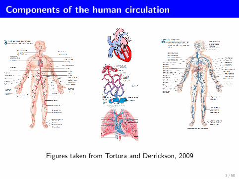
Components of the human circulation

Figures taken from Tortora and Derrickson, 2009

3 / 50

Fluid-Structure Interaction (FSI) models

• 3D Navier-Stokes equations for blood flow in compliant vessels

• 3D equations for the dynamics of the structure (vessel solid wall)

• Interaction (coupling) of these systems

• Advantages/disadvantages

• Can resolve local details on rheology, vascular wall dynamics, flowvelocity in 3D, etc

• Desing of numerical algorithms is challenging

• High computational cost

• FSI models can only be used locally, perhaps coupled to other, simplermodels

4 / 50

One-dimensonal models

• The unknowns are integral averages of flow quantities at each sectionof the vessel:

• cross-sectional area (not shape)• velocity• flow• pressure

These quantities are time-dependent and space-dependent along thelength of the vessel

• Equations are a non-linear system two equations with source terms

• A closure condition is needed: the tube law

• Wave propagation phenomena in the vascular network is resolved here

• Much lower computational cost than for full FSI models

• These models may be interpreted as representing a telegraphicnetwork along which signals are transmitted: nutrients, biologicalsignals, waste removal

5 / 50

Zero-dimensional models

• Also called lumped parameter or compartmental models

• Analogy with Kirchhoff laws for hydraulic networks is used, or electricanalogues

• These models use Ordinary Differential equations (ODEs), or moreprecisely, Differential Algebraic Equations (DAEs)

• There is no space resolution, just time variation of quantities

• No resolution of wave propagation phenomena

• These are the cheaper models and can still account for physiologicaleffect such as regulatory mechanisms

• Suitable for the capillary bed and the heart, for example

6 / 50

Geometrical multi-scale approach

• Accounting for blood flow in the complete network of vessels(millions), with very different dimensions (spatial scales), is animpossible computational task today

• A feasible approach is the Geometrical multi-scale approach: use 1-Dmodels in all major vessels, 0-D models for the microvasculature andFSI models for special districts (organs) of interest for higherdefinition

• Linking (coupling or matching conditions) these models correctly ischallenging, both from the mathematical and numerical points ofview

• Here we shall adopt the geometric multi-scale models involving 1-Dand 0-D submodels

7 / 50

The incompressible Navier-Stokesequations

8 / 50

The incompressible Navier-Stokes equations

In full, the three-dimensional, time-dependent incompressibleNavier-Stokes equations are

∂xu+ ∂yv + w∂zw = 0

∂tu+ u∂xu+ v∂yu+ w∂zu+ 1ρ∂xp = g(x) + µ

ρ (∂2xu+ ∂2yu+ ∂2zu)

∂tv + u∂xv + v∂yv + w∂zv + 1ρ∂yp = g(y) + µ

ρ (∂2xv + ∂2yv + ∂2zv)

∂tw + u∂xw + v∂yw + w∂zw + 1ρ∂zp = g(z) + µ

ρ (∂2xw + ∂2yw + ∂2zw)

(1)

Here the four unknowns are

U(x, y, z, t) = (u, v, w): Velocity vector ,

p(x, y, z, t): Pressure .

(2)

9 / 50

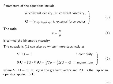
Parameters of the equations include:

ρ: constant density , µ: constant viscosity ,

G = (g(x), g(y), g(z)): external force vector

(3)

The ratioν =

µ

ρ(4)

is termed the kinematic viscosity.

The equations (1) can also be written more succinctly as

∇ ·U = 0 : continuity

∂tU + (U · ∇)U + 1ρ∇p = 1

ρ∆U + G : momentum

(5)

where ∇ ·U = divU, ∇p is the gradient vector and ∆U is the Laplacianoperator applied to U.

10 / 50

Formulations of the equations

We study three mathematical formulations of the governing equations inCartesian coordinates and restrict our attention to the two-dimensionalcase, namely

∂xu+ ∂xv = 0 , (6)

∂tu+ u∂xu+ v∂yu+1

ρ∂xp = ν

[∂2xu+ ∂2yu

], (7)

∂tv + u∂xv + v∂yv +1

ρ∂yp = ν

[∂2xv + ∂2yv

]. (8)

We have a set of three equations (6)-(8) for the three unknowns u, v, p. Inprinciple, given a domain along with initial and boundary conditions forthe equations one should be able to solve this problem.

11 / 50

The stream function-vorticity formulation

This formulation is attractive for the two-dimensional case but not somuch in three dimensions, in which the role of a stream function isreplaced by that of a vector potential. The magnitude of the vorticityvector can be written as

ζ = ∂xv − ∂yu . (9)

Introducing a stream function ψ we have

u = ∂yψ , v = −∂xψ . (10)

By combining equations (7) and (8), so as to eliminate pressure p, andusing (9) we obtain

∂tζ + u∂xζ + v∂yζ = ν[∂2xζ + ∂2yζ

], (11)

which is called the vorticity transport equation (advection-diffusion,parabolic type).

12 / 50

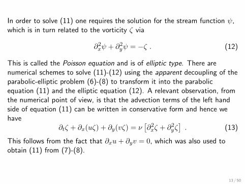
In order to solve (11) one requires the solution for the stream function ψ,which is in turn related to the vorticity ζ via

∂2xψ + ∂2yψ = −ζ . (12)

This is called the Poisson equation and is of elliptic type. There arenumerical schemes to solve (11)-(12) using the apparent decoupling of theparabolic-elliptic problem (6)-(8) to transform it into the parabolicequation (11) and the elliptic equation (12). A relevant observation, fromthe numerical point of view, is that the advection terms of the left handside of equation (11) can be written in conservative form and hence wehave

∂tζ + ∂x(uζ) + ∂y(vζ) = ν[∂2xζ + ∂2yζ

]. (13)

This follows from the fact that ∂xu+ ∂yv = 0, which was also used toobtain (11) from (7)-(8).

13 / 50

The Artificial Compressibility Equations

This is yet another approach to formulate the incompressibleNavier-Stokes equations and was originally put forward by Chorin [1] forthe steady case. See also [3].

Consider the two-dimensional equations (6)-(8) in non-dimensional form

∂xu+ ∂yv = 0 , (14)

∂tu+ u∂xu+ v∂yu+ ∂xp = α[∂2xu+ ∂2yu

], (15)

∂tv + u∂xv + v∂yv + ∂yp = α[∂2xv + ∂2yv

], (16)

where the following non-dimensionalisation has been used.

u← u/V∞ , v ← v/V∞ , p← pρ∞V 2

∞,

x← x/L , y ← y/L , t← tV∞/L ,

α = 1/ReL , ReL = V∞Lν∞

.

(17)

14 / 50

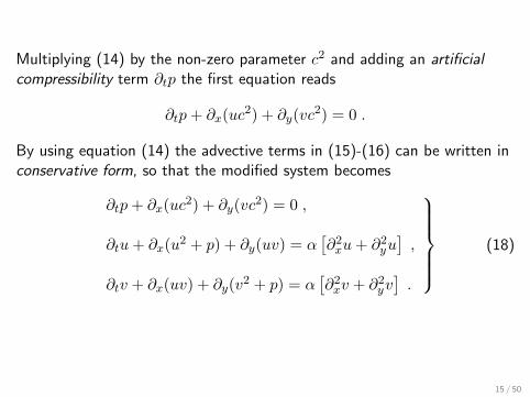
Multiplying (14) by the non-zero parameter c2 and adding an artificialcompressibility term ∂tp the first equation reads

∂tp+ ∂x(uc2) + ∂y(vc2) = 0 .

By using equation (14) the advective terms in (15)-(16) can be written inconservative form, so that the modified system becomes

∂tp+ ∂x(uc2) + ∂y(vc2) = 0 ,

∂tu+ ∂x(u2 + p) + ∂y(uv) = α[∂2xu+ ∂2yu

],

∂tv + ∂x(uv) + ∂y(v2 + p) = α

[∂2xv + ∂2yv

].

(18)

15 / 50

These equations can be written in compact form as

∂tQ + ∂xF(Q) + ∂yG(Q) = D , (19)

where

Q =

puv

, F =

c2uu2 + puv

,

G =

c2vuv

v2 + p

, D =

0α(∂2xu+ ∂2yu

)α(∂2xv + ∂2yv

) .

(20)

Equations (19)-(20) are called the artificial compressibility equations. Herec2 is the artificial compressibility factor, a constant parameter. The sourceterm vector in this case is a function of second derivatives. Note that themodified equations are equivalent to the original equations in the steadystate limit.

16 / 50

• The left-hand side of (19)-(20) form a non-linear hyperbolic system

• The Riemann problem can be defined and solved exactly orapproximately. See [2]

• Once a Riemann solver is available one can deploy Godunov-typenumerical methods to solve the equations

17 / 50

The one-dimensional equations

18 / 50

Reynolds theorem applied to a blood vessel

Consider a generic blood vessel with axial coordinate x, as shown in Fig. 1

x

z

y

Sw(x, y, z, t)

V (t)

sL(xL, y, z, t) sR(xR, y, z, t)s(x, y, z, t)

x = xL x = xRx

bbb

Fig. 1. Sketch of section of blood vessel in three dimensions defining control volume V (t) with boundary S(t).

• s(x, y, z, t): generic cross section at x

• sL: left cross section at x = xL, fixed, normal to direction x

• sR: right cross section at x = xR, fixed, normal to direction x

19 / 50

• Boundary S(t) of V (t) is decomposed as

S(t) = Sw ∪ {sL, sR} (21)

• Sw = Sw(x, y, z, t): vessel wall

The Reynolds transport theorem states

d

dt

∫V (t)F(x, t)dV =

∫V (t)

∂tF(x, t)dV +

∫S(t)FUb · ndσ (22)

• Ub: velocity of boundary S(t)

• F(x, t): a continuous function

• x = (x, y, z)

• n: outward unit normal vector to S(t)

20 / 50

For our problem the Reynolds theorem becomes

d

dt

∫V (t)F(x, t)dV =

∫V (t)

∂tF(x, t)dV +

∫Sw

FUw · ndσ (23)

• Uw: velocity of the vessel wall Sw• Ub · n = 0 at x = xL and x = xR

Assume the general case in which there may be fluid filtration across thevessel wall (permeable wall). Then the relative velocity is

Ur = Uw −U (24)

where U = (u, v, w) is the blood velocity.

It is convenient to define the cross-sectional average of a quantity a(x, t)at section s of area A as

a =1

A

∫sa(x, t)dσ Note: A =

∫s

1dσ (25)

Obviously ∫V (t)

a(x, t)dV =

∫ xR

xL

[∫sa(x, t)dσ

]dx (26)

21 / 50

which by virtue of (25) becomes∫V (t)

a(x, t)dV =

∫ xR

xL

Aa(x, t)dx (27)

Because xL and xR are independent of time

d

dt

∫V (t)F(x, t)dV =

d

dt

∫ xR

xL

AF(x, t)dx =

∫ xR

xL

∂t(AF(x, t))dx (28)

The second term on the right-hand side of (23), in view of (24), becomes∫Sw

FUw · ndσ =

∫Sw

FUr · ndσ +

∫Sw

FU · ndσ (29)

• For an impermeable wall, the first term on RHS of (29) is zero

• In view of (21), the second term on RHS of (29) becomes∫Sw

FU · ndσ =

∫S(t)FU · ndσ −

∫SL

FU · ndσ −∫SR

FU · ndσ

(30)

22 / 50

Since u is the x component of velocity of U, then (30) becomes∫Sw

FU · ndσ =

∫S(t)FU · ndσ +

∫sL

Fudσ −∫sR

Fudσ (31)

The first term on the RHS of (31), in view of Gauss’ theorem, becomes∫S(t)FU · ndσ =

∫V (t)∇ · (FU)dV (32)

and thus (31) becomes∫Sw

FU · ndσ =

∫V (t)∇ · (FU)dV +

∫sL

Fudσ −∫sR

Fudσ (33)

23 / 50

From (25) we may write the last two terms in (33) as∫sL

Fudσ −∫sR

Fudσ = −∫ xR

xL

∂

∂x

(AFu

)dx (34)

and thus (33) becomes∫Sw

FUw · ndσ =

∫Sw

FUr · ndσ +

∫V (t)∇ · (FU)dV

−∫ xR

xL

∂

∂x

(AFu

)dx

(35)

Inserting (28) and (35) into (23) and using (26) yields∫ xR

xL

∂

∂t

(AF)dx =

∫V (t)

∂tFdV +

∫V (t)∇ · (FU)dV

+

∫Sw

FUr · ndσ −∫ xR

xL

∂

∂x

(AFu

)dx

(36)

24 / 50

That is∫ xR

xL

∂

∂t

(AF)dx =

∫ xR

xL

(∫s

∂

∂tFdσ

)dx+

∫ xR

xL

(∫s

∇ · (FU)dσ

)dx

+

∫ xR

xL

(∫∂s

FUr · ndξ)dx−

∫ xR

xL

∂

∂x

(AFu

)dx

(37)

which after rearranging becomes

∂

∂t(AF) +

∂

∂x(AFu) =

∫s

(∂

∂tF +∇ · (FU)

)dσ +

∫∂s

FUr · ndξ (38)

• The function F in (38) is open to choice

• Appropriate choices of F will give the governing blood flow equations

• For an impermeable wall the last term on RHS vanishes

25 / 50

Governing 1D equations: conservation of mass

We use the area-averaged version (38) of Reynolds transport theorem,with reference to Fig. 1.

By setting F = 1 and noting that for an incompressible fluid ∇ ·U = 0,equation (38) gives the equation of continuity or mass conservationequation

∂

∂tA+

∂

∂x(Au) =

∫∂s

Ur · ndξ (39)

which for an impermeable wall becomes homogenous (no source term)

∂

∂tA+

∂

∂x(Au) = 0 (40)

• A(x, t) is the unknown cross-sectional area

• u(x, t) is the unknown cross-section averaged velocity

26 / 50

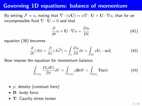
Governing 1D equations: balance of momentum

By setting F = u, noting that ∇ · (uU) = u∇ ·U + U · ∇u, that for anincompressible fluid ∇ ·U = 0 and that

∂

∂tu+ U · ∇u =

Du

Dt(41)

equation (38) becomes

∂

∂t(Au) +

∂

∂x(Au2) =

∫s

Du

Dtdσ +

∫∂s

uUr · ndξ (42)

Now impose the equation for momentum balance∫V (t)

D(ρU)

DtdV =

∫V (t)

ρBdV +

∫S(t)

Tndσ (43)

• ρ: density (constant here)

• B: body force

• T: Cauchy stress tensor27 / 50

Applying the divergence theorem to last term on RHS of (43) we obtain∫V (t)

DU

DtdV =

∫V (t)

BdV +1

ρ

∫V (t)

∇ ·TdV (44)

From the constitutive law for a fluid

T = −pI + D (45)

• p: pressure

• I: identity tensor

• D: tensor of deviatoric stresses

Equation (44) can now be written thus∫ xR

xL

(∫s

DU

DtdS

)dx =

∫ xR

xL

(∫s

[B +

1

ρ(−∇p+∇ ·D

]dσ

)dx (46)

28 / 50

For the x-component, equation (46), with obvious notation for b and d,becomes ∫

s

Du

Dtdσ =

∫s

[b+1

ρ(− ∂

∂xp+ d)]dσ (47)

Returning to (42) we have

∂

∂t(Au) +

∂

∂x(Au2) =

∫s

[b+1

ρ(− ∂

∂xp+ d)]dσ +

∫∂s

uUr · ndξ (48)

In terms of area-averages we have

∂

∂t(Au) +

∂

∂x(Au2) =

A

ρ[ρb− ∂

∂xp+ d] +

∫∂s

uUr · ndξ (49)

The Coriolis coefficient α is introduced via

α(u)2 = u2 =1

A

∫su2dσ (50)

• α depends on the assumed velocity profile

• α = 1 for a flat profile and α = 4/3 for a parabolic velocity profile29 / 50

Viscous forces are represented by d and here we assume the linear relation

A

ρd = −Ru (51)

R > 0 represents viscous resistance per unit length of tube.

Finally, the momentum equation becomes

∂

∂t(Au) +

∂

∂x(αA(u)2) +

A

ρ

∂

∂xp = Ab−Ru+

∫∂s

uUr · ndξ (52)

The governing equations are (39) and (52) and the unknowns are:

• A(x, t): cross-sectional area

• u(x, t): area-averaged velocity

• p(x, t): area averaged pressure

There are more unknowns that equations and hence a closure condition isneeded, a tube law. This will come from mechanical considerations.

30 / 50

Simplified equations

We assume an impermeable wall, zero body forces and drop bars fromunknowns. Then the continuity and momentum equations become

∂tA+ ∂x(Au) = 0

∂t(Au) + ∂x(αAu2

)+ A

ρ ∂xp = −Ru

(53)

The unknowns:

• A(x, t): cross-sectional area of vessel

• u(x, t): cross-sectional averaged velocity;

• p(x, t): cross-sectional averaged internal pressure

Flow rate:q = Au

Parameters:

• ρ: density of blood

• α: Coriolis coefficient. Here we choose α = 131 / 50

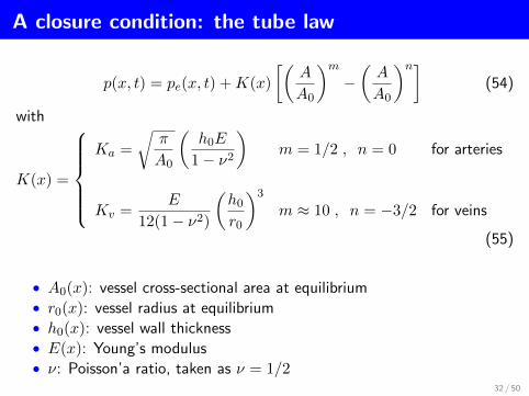
A closure condition: the tube law

p(x, t) = pe(x, t) +K(x)

[(A

A0

)m−(A

A0

)n](54)

with

K(x) =

Ka =

√π

A0

(h0E

1− ν2

)m = 1/2 , n = 0 for arteries

Kv =E

12(1− ν2)

(h0r0

)3

m ≈ 10 , n = −3/2 for veins

(55)

• A0(x): vessel cross-sectional area at equilibrium• r0(x): vessel radius at equilibrium• h0(x): vessel wall thickness• E(x): Young’s modulus• ν: Poisson’a ratio, taken as ν = 1/2

32 / 50

Tube law: arteries versus veins. Behaviour of pressure as function ofnon-dimensional cross-sectional area, for arteries and veins.

33 / 50

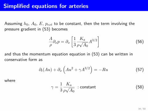
Simplified equations for arteries

Assuming h0, A0, E, pext to be constant, then the term involving thepressure gradient in (53) becomes

A

ρ∂xp = ∂x

[1

3

Ka

ρ√A0A3/2

](56)

and thus the momentum equation equation in (53) can be written inconservative form as

∂t(Au) + ∂x

(Au2 + γA3/2

)= −Ru (57)

where

γ =1

3

Ka

ρ√A0

: constant (58)

34 / 50

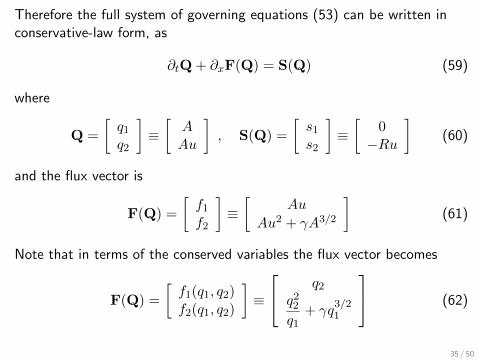
Therefore the full system of governing equations (53) can be written inconservative-law form, as

∂tQ + ∂xF(Q) = S(Q) (59)

where

Q =

[q1q2

]≡[AAu

], S(Q) =

[s1s2

]≡[

0−Ru

](60)

and the flux vector is

F(Q) =

[f1f2

]≡[

Au

Au2 + γA3/2

](61)

Note that in terms of the conserved variables the flux vector becomes

F(Q) =

[f1(q1, q2)f2(q1, q2)

]≡

q2q22q1

+ γq3/21

(62)

35 / 50

Equations for vessels with variable properties

Recall the one-dimensional equations with α = 1 read

∂tA+ ∂x(Au) = 0

∂t(Au) + ∂x(Au2

)+ A

ρ ∂xp = −Ru

(63)

along with the tube law written as

p(x, t) = pe(x, t) +K(x)ψ(A) (64)

The non-conservative term in the momentum equation can be re-written as

∂t(Au) + ∂x(Au2

)+ ∂x

pA

ρ− p

ρ∂xA = −Ru (65)

But note the following identity (see Elad etal. 1991)

− p

ρ∂xA = −1

ρ

{pe∂xA+ ∂x

[K

∫ψ(A)dA

]− ∂xK

∫ψ(A)dA

}(66)

36 / 50

Use of (66) into (65), followed by manipulations yields a conservative formfor the momentum equation and the whole system can be written as

∂tA+ ∂x(uA) = 0

∂t(Au) + ∂x

[A(u2 + p−pe

ρ

)− K

ρ

∫ψ(A)dA

]= sM

(67)

with the momentum source term given as

sM = −Ru− A

ρ∂xpe −

1

ρ∂xK

∫ψ(A)dA (68)

• The source term sM includes spatial gradients of parameters of theproblem: pe(x, t), K(x)

• These geometric-type source terms are difficult to treat numerically,specially for large gradients, or even discontinuities

37 / 50

Zero-Dimensional Equations(Lumped-Parameter Models, or

Compartmental Models)

38 / 50

The idea of 0-D models

• The concept of compartment is introduced to refer to a particulardistrict of the body

• The full body may be modelled (represented) by a finite set ofcompartments, linked in an appropriate way

• Within each compartment, haemodynamics variables are constant inspace and vary only in time (spatial homogeneity)

• In a 0-D model one studies the behaviour of a compartment inrelation to others

39 / 50

Recalling the 1D blood flow equations

The continuity and momentum equations, plus the tube law are

∂tA+ ∂xQ = 0 ,

∂tQ+ ∂x(αAu2

)+ A

ρ ∂xp = −KRu

p(x, t) = pe(x, t) +K[(

AA0

)m−(AA0

)n]

(69)

The unknowns are:

• A(x, t): cross-sectional area of vessel• u(x, t): averaged velocity; Q = Au: flow rate• p(x, t): internal pressure

Parameters:

• KR: viscous resistance of the flow per unit length of the tube• ρ: density of blood• α: Coriolis coefficient. Here we choose α = 1

40 / 50

Define spatial integral averages

Consider a segment [x1, x2] of length ∆s = x2 − x1 of a vessel and defineintegral averages

Q(t) =1

∆s

∫ x2

x1

Q(x, t)dx

p(t) =1

∆s

∫ x2

x1

p(x, t)dx

A(t) =1

∆s

∫ x2

x1

A(x, t)dx

(70)

41 / 50

The continuity equation

Integrate in space the continuity equation in the interval [x1, x2], the firstof equations (69), namely

∂tA+ ∂xQ = 0 . (71)

We obtain

∂t

(1

∆s

∫ x2

x1

A(x, t)dx

)+

1

∆s(Q(x2, t)−Q(x1, t)) = 0 . (72)

This is an ordinary differential equation (ODE) in time for the averagedcross-sectional area, namely

∆sd

dtA(t) +Q(x2, t)−Q(x1, t) = 0 . (73)

42 / 50

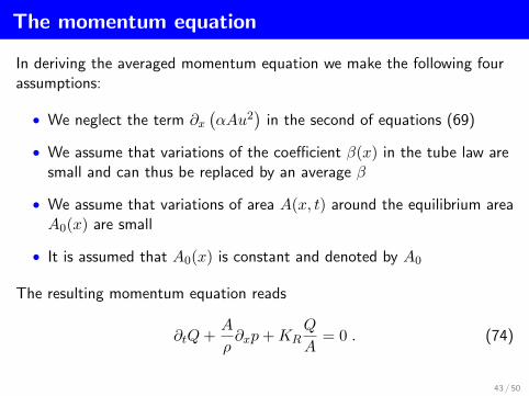
The momentum equation

In deriving the averaged momentum equation we make the following fourassumptions:

• We neglect the term ∂x(αAu2

)in the second of equations (69)

• We assume that variations of the coefficient β(x) in the tube law aresmall and can thus be replaced by an average β

• We assume that variations of area A(x, t) around the equilibrium areaA0(x) are small

• It is assumed that A0(x) is constant and denoted by A0

The resulting momentum equation reads

∂tQ+A

ρ∂xp+KR

Q

A= 0 . (74)

43 / 50

Integrating (74) term by term we obtain

1

∆s

∫ x2

x1

∂tQ(x, t)dx =d

dtQ(t)

1

∆s

∫ x2

x1

A(x, t)

ρ∂xp(x, t)dx =

A0

∆sρ[p(x2, t)− p(x1, t)]

1

∆s

∫ x2

x1

KRQ(x, t)

A(x, t)dx =

KR

A0Q(t) .

(75)

Thus the averaged momentum equation (74) becomes

∆sρ

A0

d

dtQ(t) +

∆sρKR

A20

Q(t) + p(x2, t)− p(x1, t) = 0 . (76)

44 / 50

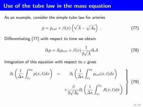
Use of the tube law in the mass equation

As an example, consider the simple tube law for arteries

p = pext + β(x)(√

A−√A0

). (77)

Differentiating (77) with respect to time we obtain

∂tp = ∂tpext + β(x)1

2√A∂tA (78)

Integration of this equation with respect to x gives

∂t

(1

∆s

∫ x2

x1

p(x, t)dx

)= ∂t

(1

∆s

∫ x2

x1

pext(x, t)dx

)

+β

2√A0∂t

(1

∆s

∫ x2

x1

A(x, t)dx

) (79)

45 / 50

Further manipulations of (79) yield a relationship between A(t) andpressure p(t), including pext(t), namely

d

dtA(t) =

2√A0

β

d

dtp(t)− 2

√A0

β

d

dtpext(t) . (80)

Substitution of (80) into (73) yields the continuity equation in the form

2√A0∆s

β

d

dtp(t) +Q(x2, t)−Q(x1, t) =

2√A0∆s

β

d

dtpext(t) (81)

46 / 50

The zero-dimensional equations

Collecting the equations (81) and (76) we obtain the system

Cd

dtp(t) +Q(x2, t)−Q(x1, t) = C

d

dtpext(t)

Ld

dtQ(t) +RQ(t) + p(x2, t)− p(x1, t) = 0

(82)

where the coefficients C, L and R are defined as

C =2√A0∆s

βCapacitance. Mass storage term due to compliance

L =ρ∆s

A0Inductance. Inertia term in the momentum equation

R =ρ∆sKR

A20

Resistance (due to viscosity and radii of vessels)

(83)

47 / 50

Recalling electric circuits

• An electric circuit: a source of electric energy (e.g. a generator) anda resistors or an inductor or a capacitor.

• Kirchhoff’s second law for the flow of current: In a closed circuit, theimpressed voltage E(t) is equal to the sum of the voltage drops E∗ inthe rest of the circuits

• Experiments give

Resistor : voltage drop across the resistor ER = RI

Inductor : voltage drop across the inductor EL = L ddtI

Capacitor : voltage drop across the capacitor EC = 1CQ

(84)

HereI(t) current (ampere)R resistance (ohms)L inductance (henrys)C capacitance (farads)

(85)

48 / 50

Analogy between blood flow and electric circuits

Haemodynamics Electric circuitPressure p Voltage E

Flow Q Current I

Blood viscosity Resistance R

Blood inertia Inductance L

Wall compliance Capacitance C

Table 1. Analogy between 0-Dimensional haemodynamics and electriccircuits.

49 / 50

REFERENCES

• J R LevickCardiovascular physiology. Hodder Arnold, Fifth Edition, 2010

• G. J. Tortora and B. DerricksonPrinciples of anatomy and physiology. John Wiley and Sons, 12thEdition, 2009.

• L Formaggia, A Quarteroni and A Veneziani (Editors)Cardiovascular mathematics. Springer 2009

• D Elad, D Katz, E Kimmel and S EinavNumerical schemes for unsteady fluid flow through collapsible tubes.J. Biomed. Eng. Vol. 13, 1991

• E Kreyszig.Advanced engineering mathematics

50 / 50

A. J. Chorin.A Numerical Method for Solving Viscous Flow Problems.J. Comput. Phys., 2:12–26, 1967.

E. F. Toro.Exact and Approximate Riemann Solvers for the ArtificialCompressibility Equations.Technical Report 97–02, Department of Mathematics and Physics,Manchester Metropolitan University, UK, 1997.

E. F. Toro.Riemann Solvers and Numerical Methods for Fluid Dynamics. APractical Introduction. Third Edition.Springer–Verlag, 2009.

50 / 50