Dieu D. Nguyen , Sebastian Kamann Michele Cappellari ... the number of low-mass galaxies with...

Draft version April 13, 2018Preprint typeset using LATEX style emulateapj v. 04/17/13

NEARBY EARLY-TYPE GALACTIC NUCLEI AT HIGH RESOLUTION – DYNAMICAL BLACK HOLE ANDNUCLEAR STAR CLUSTER MASS MEASUREMENTS

Dieu D. Nguyen1, Anil C. Seth1, Nadine Neumayer2, Sebastian Kamann3, Karina T. Voggel1,Michele Cappellari4, Arianna Picotti2, Phuong M. Nguyen5, Torsten Boker6, Victor Debattista7,

Nelson Caldwell8, Richard McDermid9, Nathan Bastian3, Christopher C. Ahn1, and Renuka Pechetti1

Draft version April 13, 2018

ABSTRACT

We present a detailed study of the nuclear star clusters (NSCs) and massive black holes (BHs) of fourof the nearest low-mass early-type galaxies: M32, NGC 205, NGC 5102, and NGC 5206. We measuredynamical masses of both the BHs and NSCs in these galaxies using Gemini/NIFS or VLT/SINFONIstellar kinematics, Hubble Space Telescope (HST ) imaging, and Jeans Anisotropic Models. We detectmassive BHs in M32, NGC 5102, and NGC 5206, while in NGC 205, we find only an upper limit. TheseBH mass estimates are consistent with previous measurements in M32 and NGC 205, while those inNGC 5102 & NGC 5206 are estimated for the first time, and both found to be <106M�. This adds tojust a handful of galaxies with dynamically measured sub-million M� central BHs. Combining theseBH detections with our recent work on NGC 404’s BH, we find that 80% (4/5) of nearby, low-mass(109 − 1010M�; σ? ∼ 20− 70 km s−1) early-type galaxies host BHs. Such a high occupation fractionsuggests the BH seeds formed in the early epoch of cosmic assembly likely resulted in abundant seeds,favoring a low-mass seed mechanism of the remnants, most likely from the first generation of massivestars. We find dynamical masses of the NSCs ranging from 2−73×106M� and compare these massesto scaling relations for NSCs based primarily on photometric mass estimates. Color gradients suggestyounger stellar populations lie at the centers of the NSCs in three of the four galaxies (NGC 205,NGC 5102, and NGC 5206), while the morphology of two are complex and are best-fit with multiplemorphological components (NGC 5102 and NGC 5206). The NSC kinematics show they are rotating,especially in M32 and NGC 5102 (V/σ? ∼ 0.7).

Subject headings: Galaxies: kinematics and dynamics – Galaxies: nuclei – Galaxies: centers – Galaxies:individual (NGC 221 (M32), NGC 205, NGC 5102, and NGC 5206

1. INTRODUCTION

Supermassive black holes (SMBHs) appear to be ubiq-uitous features of the centers of massive galaxies. Thisis inferred in nearby galaxies, both from their dynami-

1 Department of Physics and Astronomy, University of Utah,115 South 1400 East, Salt Lake City, UT 84112, [email protected], [email protected],[email protected], [email protected],[email protected]

2 Max Planck Institut fur Astronomie (MPIA), Konigstuhl17, 69121 Heidelberg, [email protected], [email protected]

3 Astrophysics Research Institute, Liverpool John MooresUniversity, 146 Brownlow Hill, Liverpool L3 5RF, [email protected], [email protected]

4 Sub-department of Astrophysics, Department of Physics,University of Oxford, Denys Wilkinson Building, Keble Road,Oxford OX1 3RH, [email protected]

5 Department of Physics, Quy Nhon University,170 An Duong Vuong, Quy Nhon, [email protected]

6 European Space Agency, c/o STScI, 3700 San Martin Drive,Baltimore, MD 21218, [email protected]

7 School of Physical Sciences and Computing, University ofCentral Lancashire, Preston, Lancashire, PR1 2HE, [email protected]

8 Harvard-Smithsonian Center for Astrophysics, HarvardUniversity, 60 Garden St, Cambridge, MA 02138, [email protected]

9 Department of Physics and Astronomy, Macquarie Univer-sity, NSW 2109, [email protected]

cal detection (see review by Kormendy & Ho 2013), andfrom the presence of accretion signatures (e.g., Ho et al.2009). Furthermore, the mass density of these BHs innearby massive galaxies is compatible with the inferredmass accretion of active galactic nuclei (AGN) in thedistant universe (e.g., Marconi et al. 2004). However,the presence of central BHs is not well constrained inlower mass galaxies, particularly below stellar masses of∼1010 M� (e.g., Greene 2012; Miller et al. 2015). Theselower mass galaxy nuclei are almost universally popu-lated by bright, compact nuclear star clusters (NSCs)(e.g., Georgiev & Boker 2014; den Brok et al. 2014b) withhalf-light/effective radius of reff ∼ 3 pc. These NSCs areknown to co-exist in some cases with massive BHs, in-cluding in the Milky Way (MW Seth et al. 2008; Graham& Spitler 2009; Neumayer & Walcher 2012).

Finding and weighing central BHs in lower mass galax-ies is challenging due to the difficulty of dynamically de-tecting the low-mass (.106M�) BHs they host. How-ever, it is a key measurement for addressing several re-lated science topics. First, low-mass galaxies are abun-dant (e.g., Blanton et al. 2005), and thus if they com-monly host BHs, these will dominate the number density(but not mass density) of BHs in the local universe. Thishas consequences for a wide range of studies, from theexpected rate of tidal disruptions (Kochanek 2016), tothe number of BHs we expect to find in stripped galaxynuclei (e.g., Pfeffer et al. 2014; Ahn et al. 2017). Sec-ond, the number of low-mass galaxies with central BHs

arX

iv:1

711.

0431

4v2

[as

tro-

ph.G

A]

12

Apr

201

8

is currently most feasible way to probe the unknown for-mation mechanism of massive BHs. More specifically, ifmassive BHs form from the direct collapse of relativelymassive ∼105M� seed black holes scenario (e.g., Lodato& Natarajan 2006; Bonoli et al. 2014), few would beexpected to inhabit low-mass galaxies, if, on the otherhand, they form from the remnants of Population IIIstars, a much higher “occupation fraction” is expected inlow-mass galaxies (Volonteri et al. 2008; van Wassenhoveet al. 2010; Volonteri 2010). This work is complementaryto work that is starting to be undertaken at higher red-shifts to probe accreting black holes at the earliest epochs(e.g., Weigel et al. 2015; Natarajan et al. 2017; Volonteriet al. 2017). Tidal disruptions are also starting to probethe BH population of low mass galaxies (e.g., Weverset al. 2017; Law-Smith et al. 2017), and may eventuallyprovide constraints on occupation fraction (e.g., Stone &Metzger 2016). Third, dynamical mass measurements ofSMBHs (MSMBH ∼ 106−1010M�) have shown that theirmasses scale with the properties of their host galaxiessuch as their bulge luminosity, bulge mass, and veloc-ity dispersion (Kormendy & Ho 2013; McConnell & Ma2013; Graham & Scott 2015; Saglia et al. 2016). Thesescaling relations have been used to suggest that galaxiesand their central SMBHs coevolve, likely due to feedbackfrom the AGN radiation onto the surrounding gas (seereview by Fabian 2012).

The black hole–galaxy relations are especially tightfor massive early-type galaxies (ETGs), while later-type,lower dispersion galaxies show a much larger scatter(Greene et al. 2016; Lasker et al. 2016b). However, thelack of measurements at the low-mass, low-dispersionend, especially in ETGs means that our knowledge ofhow BHs populate host galaxies is very incomplete.

The population of known BHs in low-mass galaxies wasrecently compiled by Reines & Volonteri (2015). Of theBHs known in galaxies with stellar masses <1010M�,most have been found by the detection of optical broad-line emission, with their masses inferred from the velocitywidths of their broad-lines (e.g., Greene & Ho 2007; Donget al. 2012; Reines et al. 2013). Many of these galaxieshost BHs with inferred masses below 106M�, especiallythose with stellar mass .3×109M�. Broad-line emissionis however found in only a tiny fraction (<1%) of low-mass galaxies; other accretion signatures that are alsouseful for identifying BHs in low-mass galaxies includenarrow-line emission (e.g., Moran et al. 2014), coronalemission in the mid-infrared (e.g., Satyapal et al. 2009),tidal-disruption events (e.g., Maksym et al. 2013), andhard X-ray emission (e.g., Miller et al. 2015; She et al.2017).

The current record holder for the lowest mass centralBH in a late-type galaxy (LTG) is the broad-line AGN inRGG 118 withM? ∼ 2×109 M� (MBH = 5×104M�; Bal-dassare et al. 2015). The lowest-mass systems known tohost central massive BHs are ultracompact dwarfs, whichare likely stripped galaxy nuclei (Seth et al. 2014; Ahnet al. 2017). Apart from these systems, the lowest massBH-hosting galaxies are the M? ∼ 3×108 M� early-typedwarf in Abell 1795, where a central BH is suggestedby the detection of a tidal-disruption event (Maksymet al. 2013), and the similar mass dwarf elliptical galaxyPox 52, which hosts a broad-line AGN (Barth et al. 2004;

Thornton et al. 2008). Currently, there are only a fewgalaxies with sub-million solar mass dynamical BH massestimates, including NGC 4395 (MBH = 4+8

−3 × 105M�;

den Brok et al. 2015), NGC 404 (MBH . 1.5 × 105M�;Nguyen et al. 2017), and NGC 4414 (MBH . 1.6 ×106M�; Thater et al. 2017).

Unlike BHs, the morphologies, stellar populations, andkinematics of NSCs provide an observable record for un-derstanding mass accretion into the central parsecs ofgalaxies. The NSCs’ stellar mass accretion can be dueto (1) the migration of massive star clusters formed atlarger radii that then fall into the galactic center via dy-namical friction (e.g., Lotz et al. 2001; Antonini 2013;Guillard et al. 2016) or (2) the in-situ formation of starsfrom gas that falls into the nucleus (e.g., Seth et al. 2006;Antonini et al. 2015b). Observations suggest the forma-tion of NSCs is ongoing, as they typically have multiplepopulations (e.g., Rossa et al. 2006; Nguyen et al. 2017).Most studies on NSCs in ETGs have focused on galaxiesin nearby galaxy clusters (Walcher et al. 2006); spectro-scopic and photometric studies suggest that typically theNSCs in these ETGs are younger than their surroundinggalaxy, especially in galaxies . 2 × 109 M� (e.g., Coteet al. 2006; Paudel et al. 2011; Krajnovic et al. 2017;Spengler et al. 2017). There is also a clear change in thescaling relations between NSC and galaxy luminositiesand masses at about this mass, with the scaling beingshallower at lower masses and steeper at higher masses(Scott et al. 2013; den Brok et al. 2014b; Spengler et al.2017). This change in addition to the flattening of moreluminous NSCs (Spengler et al. 2017) suggests a possiblechange in the formation mechanism of NSCs from mi-gration to in-situ formation. However, the NSC scalingrelations for ETGs are based almost entirely of photo-metric estimates, with a significant sample of dynamicalmeasurements available only for nearby late-type spirals(Walcher et al. 2005) and only two in ETG FCC 277(Lyubenova et al. 2013) and NGC 404 (Nguyen et al.2017).

The relationship between NSCs and BHs is not wellunderstood. The sample of objects with both a detectedNSC and BH is quite limited (Seth et al. 2008; Graham &Spitler 2009; Neumayer & Walcher 2012; Georgiev et al.2016), but even from this data it is clear that low-massgalaxy nuclei are typically dominated by NSCs, whilehigh mass galaxy nuclei are dominated by SMBHs. Thistransition could be due to a number of mechanisms,including the tidal disruption of infalling clusters (Fer-rarese et al. 2006; Antonini et al. 2015a), the growth ofBH seeds in more massive galaxies by tidal disruptionof stars (Stone et al. 2017), or differences in feedbackfrom star formation vs. AGN accretion (Nayakshin et al.2009). In addition, the formation of NSCs and BHs couldbe explicitly linked with NSCs creating the needed initialseed BHs during formation (e.g., Portegies Zwart et al.2004), or strong gas inflow creating the NSC and BH si-multaneously (Hopkins & Quataert 2010). However, theexistence of a BH around which a NSC appears to becurrently forming in the nearby galaxy Henize 2-10 sug-gests that BHs can form independently of NSCs (Nguyenet al. 2014).

This work presents a dynamical study of the BHs andNSCs of four nearby low-mass ETGs including the two

2

brightest companions of Andromeda, M32 and NGC 205,and two companions of Cen A, NGC 5102 and NGC 5206.Of these four galaxies, previous BH mass estimates existfor two; the detection of (2.5± 0.5)× 106M� BH in M32(Verolme et al. 2002; van den Bosch & de Zeeuw 2010),and the upper limit of 3.8×104M� (at 3σ) in NGC 205(Valluri et al. 2005). In this paper, we use adaptive op-tics integral field spectroscopic measurements, combinedwith dynamical modeling using carefully constructedmass models to constrain the BH and NSC masses inall four galaxies, including the first published constraintson the BHs of NGC 5102 and NGC 5206.

This paper is organized into nine sections. In Section 2,we describe the observations and data reduction. Thefour galaxies’ properties are presented in Section 3, andwe construct luminosity and mass models in Section 4.We present kinematics measurements of their nuclei inSection 5. We model these kinematics using Jeans mod-els and present the BH constraints and uncertainties inSection 6. In section 7 we analyze the properties of theNSCs and present our measurements of their masses. Wediscuss our results in Section 8, and conclude in Section 9.

2. DATA AND DATA REDUCTION

2.1. HST Imaging

The HST/WFPC2 PC and ACS/HRC imaging we usein this work is summarized in Table 1. The nuclei ofM32 and NGC 5206 are observed in the WFPC2 PCchip in F555W and F814W filters. For NGC 205, we usethe central ACS/HRC F555W and F814W images. ForNGC 5102, we use more imaging of WFPC2 includingtwo central saturated F450W and F560W, unsaturatedF547M, and Hα emission F656N.

For the ACS/HRC data we downloaded reduced,drizzled images from the HST/Hubble Legacy Archive(HLA). However, because the HLA images of theWFPC2 PC chip have a pixel-scale that is downgradedby 10%, we re-reduce images, which are downloaded fromthe Mikulski Archive for Space Telescope (MAST), usingAstrodrizzle (Avila et al. 2012) to a final pixel scaleof 0.′′0445. For all images, we constrain the sky back-ground by comparing them to ground-based data (seeSection 4.1).

We use the centroid positions of the nuclei to alignimages from all HST filters to the F814W (in M32,NGC 205, and NGC 5206) or F547M (in NGC 5102)data. The astrometric alignment of the Gemini/NIFSor VLT/SINFONI spectroscopic data (Section 2.2) wasthen also tied to the same images, providing a commonreference frame for all images used in this study.

2.2. Integral-Field Spectroscopic Data

2.2.1. Gemini/NIFS Spectroscopy

M32 and NGC 205 were observed with Gemini/NIFSusing the Altair tip-tilt laser guide star system. TheM32 data were previously presented in Seth (2010). Theobservational information can be found in Table 2. Weuse these data to derive stellar kinematics from the COband-head absorption in Section 5.

The data were reduced using the IRAF pipeline modi-fied to propagate the error spectrum, for details see Sethet al. (2010). The telluric calibration was done with A0Vstars, for M32, HIP 116449 was used (Seth 2010), while

for NGC 205 we use HIP 52877. The final cubes wereconstructed via a combination of six (M32) and eight(NGC 205) dithered on-source cubes with good imagequality after subtracting offset sky exposures. The wave-length calibration used both an arc lamp image and theskylines in the science exposures with an absolute errorof ∼2 km s−1.

2.2.2. VLT/SINFONI Spectroscopy

NGC 5102 and NGC 5206 were observed with SIN-FONI (Eisenhauer et al. 2003; Bonnet et al. 2004) on theUT4 (Yepun) of the European Southern Observatory’sVery Large Telescope (ESO VLT) at Cerro Paranal,Chile. NGC 5102 was observed in two consecutive nightsin March 2007 as part of the SINFONI GTO program(PI: Bender). A total of 12 on-source exposures of 600sintegration time were observed in the two nights usingthe 100 mas pixel scale. NGC 5206 was observed in ser-vice mode in three different years (2011, 2013, and 2014;PI: Neumayer) with three on-source exposures of 600s ineach of the runs. Both of the targets were observed usingthe laser guide star for the adaptive optics correction andused the NSC itself for the tip-tilt correction. The spec-tra were taken in K–band (1.93–2.47µm) at a spectralresolution of R ∼ 4000, covering a field of view of 3′′×3′′.The data were reduced using the ESO SINFONI data re-duction pipeline, following the steps (1) sky-subtraction,(2) flat-fielding, (3) bad pixel correction, (4) distortioncorrection, (5) wavelength calibration, (6) cube recon-struction, and finally (8) telluric correction. Details onthese steps are given in Neumayer et al. (2007). The fi-nal data cubes were constructed via a combination of theindividual dithered cubes. This leads to a total exposuretime of 7200s for NGC 5102 and 5400s for NGC 5206.

2.3. Point-Spread Function Determinations

Our analysis requires careful characterization of thepoint-spread functions (PSFs) in both our kinematic andimaging data. The HST PSFs are used in fitting thetwo-dimensional (2D) surface brightness profiles of thegalaxies (GALFIT; Peng et al. 2010), while the Gem-ini/NIFS and VLT/SINFONI PSFs are used for the dy-namical modeling.

For the HST PSFs, we create the model PSF for eachHST exposure using the Tiny Tim routine for each in-volved individual filter for each object. The PSFs arecreated using the tiny1 and tiny2 tasks (Krist 1995;Krist et al. 2011). We next insert these into corre-sponding c0m (M32, NGC 5102, and NGC 5206) or flt(NGC 205) images at the positions of the nucleus in eachindividual exposure to simulate our observations and useAstrodrizzle to create our final PSF as described inden Brok et al. (2015) and Nguyen et al. (2017).

For the PSFs of our integral field spectra, we convolvethe HST images with an additional broadening to de-termine the two component PSF expected from adap-tive optics observations. The Gemini/NIFS PSFs forM32 and NGC 205 are estimated as described in Sethet al. (2010). First, the outer shape of the PSF was con-strained using images of the telluric calibrator Moffatprofile (Σ(r) = Σ0/[(1 + (r/rd)

2)]4.765). We then con-volved the HST images with a inner Gaussian + outerMoffat function (with fixed shape but free amplitude) to

3

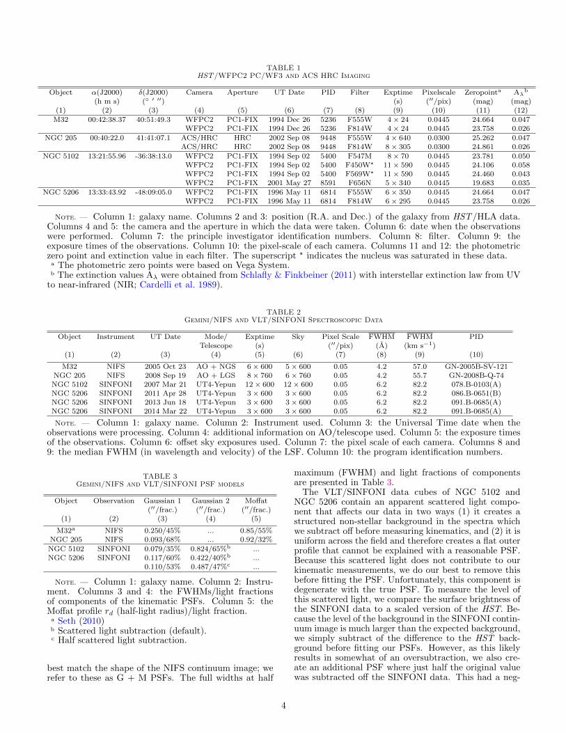
TABLE 1HST/WFPC2 PC/WF3 and ACS HRC Imaging

Object α(J2000) δ(J2000) Camera Aperture UT Date PID Filter Exptime Pixelscale Zeropointa Aλb

(h m s) (◦ ′ ′′) (s) (′′/pix) (mag) (mag)(1) (2) (3) (4) (5) (6) (7) (8) (9) (10) (11) (12)

M32 00:42:38.37 40:51:49.3 WFPC2 PC1-FIX 1994 Dec 26 5236 F555W 4 × 24 0.0445 24.664 0.047WFPC2 PC1-FIX 1994 Dec 26 5236 F814W 4 × 24 0.0445 23.758 0.026

NGC 205 00:40:22.0 41:41:07.1 ACS/HRC HRC 2002 Sep 08 9448 F555W 4 × 640 0.0300 25.262 0.047ACS/HRC HRC 2002 Sep 08 9448 F814W 8 × 305 0.0300 24.861 0.026

NGC 5102 13:21:55.96 -36:38:13.0 WFPC2 PC1-FIX 1994 Sep 02 5400 F547M 8 × 70 0.0445 23.781 0.050WFPC2 PC1-FIX 1994 Sep 02 5400 F450W? 11 × 590 0.0445 24.106 0.058WFPC2 PC1-FIX 1994 Sep 02 5400 F569W? 11 × 590 0.0445 24.460 0.043WFPC2 PC1-FIX 2001 May 27 8591 F656N 5 × 340 0.0445 19.683 0.035

NGC 5206 13:33:43.92 -48:09:05.0 WFPC2 PC1-FIX 1996 May 11 6814 F555W 6 × 350 0.0445 24.664 0.047WFPC2 PC1-FIX 1996 May 11 6814 F814W 6 × 295 0.0445 23.758 0.026

Note. — Column 1: galaxy name. Columns 2 and 3: position (R.A. and Dec.) of the galaxy from HST/HLA data.Columns 4 and 5: the camera and the aperture in which the data were taken. Column 6: date when the observationswere performed. Column 7: the principle investigator identification numbers. Column 8: filter. Column 9: theexposure times of the observations. Column 10: the pixel-scale of each camera. Columns 11 and 12: the photometriczero point and extinction value in each filter. The superscript ? indicates the nucleus was saturated in these data.

a The photometric zero points were based on Vega System.b The extinction values Aλ were obtained from Schlafly & Finkbeiner (2011) with interstellar extinction law from UV

to near-infrared (NIR; Cardelli et al. 1989).

TABLE 2Gemini/NIFS and VLT/SINFONI Spectroscopic Data

Object Instrument UT Date Mode/ Exptime Sky Pixel Scale FWHM FWHM PIDTelescope (s) (′′/pix) (A) (km s−1)

(1) (2) (3) (4) (5) (6) (7) (8) (9) (10)

M32 NIFS 2005 Oct 23 AO + NGS 6 × 600 5 × 600 0.05 4.2 57.0 GN-2005B-SV-121NGC 205 NIFS 2008 Sep 19 AO + LGS 8 × 760 6 × 760 0.05 4.2 55.7 GN-2008B-Q-74NGC 5102 SINFONI 2007 Mar 21 UT4-Yepun 12 × 600 12 × 600 0.05 6.2 82.2 078.B-0103(A)NGC 5206 SINFONI 2011 Apr 28 UT4-Yepun 3 × 600 3 × 600 0.05 6.2 82.2 086.B-0651(B)NGC 5206 SINFONI 2013 Jun 18 UT4-Yepun 3 × 600 3 × 600 0.05 6.2 82.2 091.B-0685(A)NGC 5206 SINFONI 2014 Mar 22 UT4-Yepun 3 × 600 3 × 600 0.05 6.2 82.2 091.B-0685(A)

Note. — Column 1: galaxy name. Column 2: Instrument used. Column 3: the Universal Time date when theobservations were processing. Column 4: additional information on AO/telescope used. Column 5: the exposure timesof the observations. Column 6: offset sky exposures used. Column 7: the pixel scale of each camera. Columns 8 and9: the median FWHM (in wavelength and velocity) of the LSF. Column 10: the program identification numbers.

TABLE 3Gemini/NIFS and VLT/SINFONI PSF models

Object Observation Gaussian 1 Gaussian 2 Moffat(′′/frac.) (′′/frac.) (′′/frac.)

(1) (2) (3) (4) (5)

M32a NIFS 0.250/45% ... 0.85/55%NGC 205 NIFS 0.093/68% ... 0.92/32%

NGC 5102 SINFONI 0.079/35% 0.824/65%b ...NGC 5206 SINFONI 0.117/60% 0.422/40%b ...

0.110/53% 0.487/47%c ...

Note. — Column 1: galaxy name. Column 2: Instru-ment. Columns 3 and 4: the FWHMs/light fractionsof components of the kinematic PSFs. Column 5: theMoffat profile rd (half-light radius)/light fraction.

a Seth (2010)b Scattered light subtraction (default).c Half scattered light subtraction.

best match the shape of the NIFS continuum image; werefer to these as G + M PSFs. The full widths at half

maximum (FWHM) and light fractions of componentsare presented in Table 3.

The VLT/SINFONI data cubes of NGC 5102 andNGC 5206 contain an apparent scattered light compo-nent that affects our data in two ways (1) it creates astructured non-stellar background in the spectra whichwe subtract off before measuring kinematics, and (2) it isuniform across the field and therefore creates a flat outerprofile that cannot be explained with a reasonable PSF.Because this scattered light does not contribute to ourkinematic measurements, we do our best to remove thisbefore fitting the PSF. Unfortunately, this component isdegenerate with the true PSF. To measure the level ofthis scattered light, we compare the surface brightness ofthe SINFONI data to a scaled version of the HST. Be-cause the level of the background in the SINFONI contin-uum image is much larger than the expected background,we simply subtract of the difference to the HST back-ground before fitting our PSFs. However, as this likelyresults in somewhat of an oversubtraction, we also cre-ate an additional PSF where just half the original valuewas subtracted off the SINFONI data. This had a neg-

4

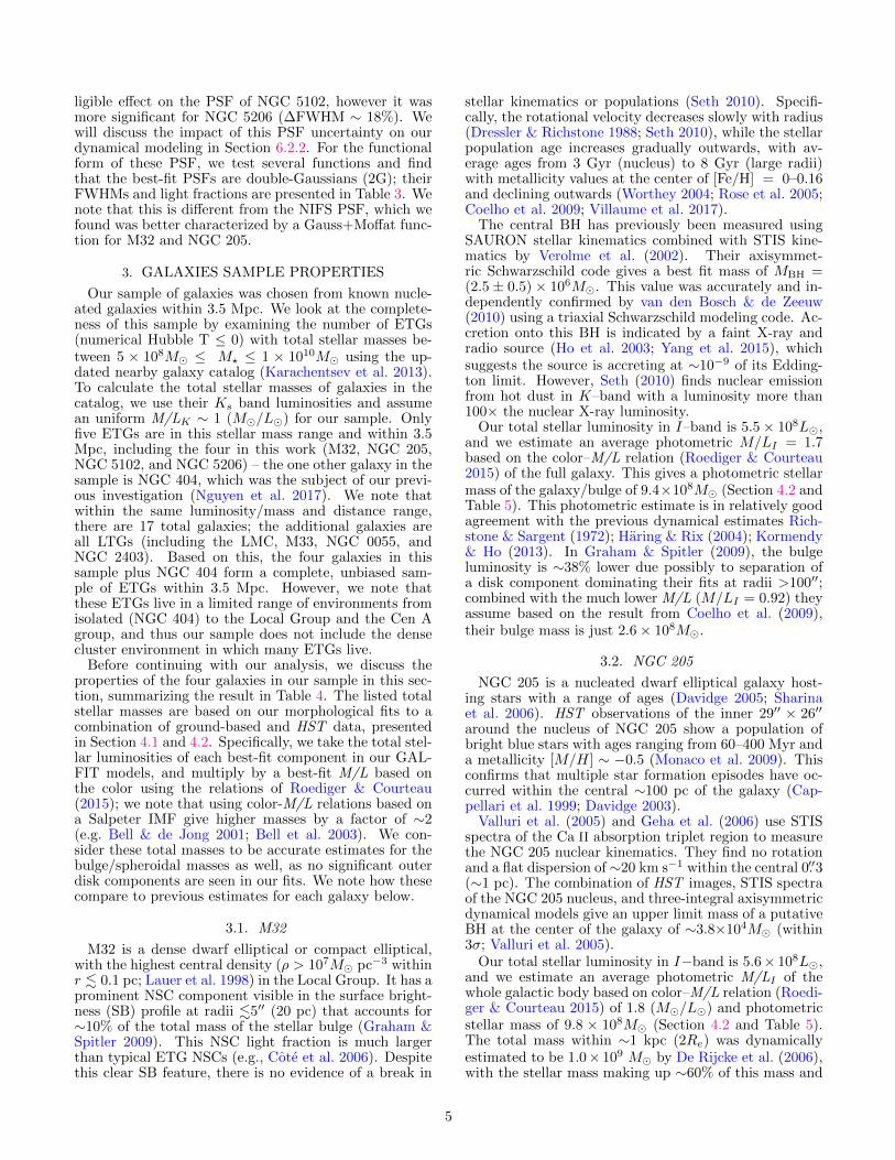
ligible effect on the PSF of NGC 5102, however it wasmore significant for NGC 5206 (∆FWHM ∼ 18%). Wewill discuss the impact of this PSF uncertainty on ourdynamical modeling in Section 6.2.2. For the functionalform of these PSF, we test several functions and findthat the best-fit PSFs are double-Gaussians (2G); theirFWHMs and light fractions are presented in Table 3. Wenote that this is different from the NIFS PSF, which wefound was better characterized by a Gauss+Moffat func-tion for M32 and NGC 205.

3. GALAXIES SAMPLE PROPERTIES

Our sample of galaxies was chosen from known nucle-ated galaxies within 3.5 Mpc. We look at the complete-ness of this sample by examining the number of ETGs(numerical Hubble T ≤ 0) with total stellar masses be-tween 5 × 108M� ≤ M? ≤ 1 × 1010M� using the up-dated nearby galaxy catalog (Karachentsev et al. 2013).To calculate the total stellar masses of galaxies in thecatalog, we use their Ks band luminosities and assumean uniform M/LK ∼ 1 (M�/L�) for our sample. Onlyfive ETGs are in this stellar mass range and within 3.5Mpc, including the four in this work (M32, NGC 205,NGC 5102, and NGC 5206) – the one other galaxy in thesample is NGC 404, which was the subject of our previ-ous investigation (Nguyen et al. 2017). We note thatwithin the same luminosity/mass and distance range,there are 17 total galaxies; the additional galaxies areall LTGs (including the LMC, M33, NGC 0055, andNGC 2403). Based on this, the four galaxies in thissample plus NGC 404 form a complete, unbiased sam-ple of ETGs within 3.5 Mpc. However, we note thatthese ETGs live in a limited range of environments fromisolated (NGC 404) to the Local Group and the Cen Agroup, and thus our sample does not include the densecluster environment in which many ETGs live.

Before continuing with our analysis, we discuss theproperties of the four galaxies in our sample in this sec-tion, summarizing the result in Table 4. The listed totalstellar masses are based on our morphological fits to acombination of ground-based and HST data, presentedin Section 4.1 and 4.2. Specifically, we take the total stel-lar luminosities of each best-fit component in our GAL-FIT models, and multiply by a best-fit M/L based onthe color using the relations of Roediger & Courteau(2015); we note that using color-M/L relations based ona Salpeter IMF give higher masses by a factor of ∼2(e.g. Bell & de Jong 2001; Bell et al. 2003). We con-sider these total masses to be accurate estimates for thebulge/spheroidal masses as well, as no significant outerdisk components are seen in our fits. We note how thesecompare to previous estimates for each galaxy below.

3.1. M32

M32 is a dense dwarf elliptical or compact elliptical,with the highest central density (ρ > 107M� pc−3 withinr . 0.1 pc; Lauer et al. 1998) in the Local Group. It has aprominent NSC component visible in the surface bright-ness (SB) profile at radii .5′′ (20 pc) that accounts for∼10% of the total mass of the stellar bulge (Graham &Spitler 2009). This NSC light fraction is much largerthan typical ETG NSCs (e.g., Cote et al. 2006). Despitethis clear SB feature, there is no evidence of a break in

stellar kinematics or populations (Seth 2010). Specifi-cally, the rotational velocity decreases slowly with radius(Dressler & Richstone 1988; Seth 2010), while the stellarpopulation age increases gradually outwards, with av-erage ages from 3 Gyr (nucleus) to 8 Gyr (large radii)with metallicity values at the center of [Fe/H] = 0–0.16and declining outwards (Worthey 2004; Rose et al. 2005;Coelho et al. 2009; Villaume et al. 2017).

The central BH has previously been measured usingSAURON stellar kinematics combined with STIS kine-matics by Verolme et al. (2002). Their axisymmet-ric Schwarzschild code gives a best fit mass of MBH =(2.5 ± 0.5) × 106M�. This value was accurately and in-dependently confirmed by van den Bosch & de Zeeuw(2010) using a triaxial Schwarzschild modeling code. Ac-cretion onto this BH is indicated by a faint X-ray andradio source (Ho et al. 2003; Yang et al. 2015), whichsuggests the source is accreting at ∼10−9 of its Edding-ton limit. However, Seth (2010) finds nuclear emissionfrom hot dust in K–band with a luminosity more than100× the nuclear X-ray luminosity.

Our total stellar luminosity in I–band is 5.5× 108L�,and we estimate an average photometric M/LI = 1.7based on the color–M/L relation (Roediger & Courteau2015) of the full galaxy. This gives a photometric stellarmass of the galaxy/bulge of 9.4×108M� (Section 4.2 andTable 5). This photometric estimate is in relatively goodagreement with the previous dynamical estimates Rich-stone & Sargent (1972); Haring & Rix (2004); Kormendy& Ho (2013). In Graham & Spitler (2009), the bulgeluminosity is ∼38% lower due possibly to separation ofa disk component dominating their fits at radii >100′′;combined with the much lower M/L (M/LI = 0.92) theyassume based on the result from Coelho et al. (2009),their bulge mass is just 2.6× 108M�.

3.2. NGC 205

NGC 205 is a nucleated dwarf elliptical galaxy host-ing stars with a range of ages (Davidge 2005; Sharinaet al. 2006). HST observations of the inner 29′′ × 26′′

around the nucleus of NGC 205 show a population ofbright blue stars with ages ranging from 60–400 Myr anda metallicity [M/H] ∼ −0.5 (Monaco et al. 2009). Thisconfirms that multiple star formation episodes have oc-curred within the central ∼100 pc of the galaxy (Cap-pellari et al. 1999; Davidge 2003).

Valluri et al. (2005) and Geha et al. (2006) use STISspectra of the Ca II absorption triplet region to measurethe NGC 205 nuclear kinematics. They find no rotationand a flat dispersion of ∼20 km s−1 within the central 0.′′3(∼1 pc). The combination of HST images, STIS spectraof the NGC 205 nucleus, and three-integral axisymmetricdynamical models give an upper limit mass of a putativeBH at the center of the galaxy of ∼3.8×104M� (within3σ; Valluri et al. 2005).

Our total stellar luminosity in I−band is 5.6× 108L�,and we estimate an average photometric M/LI of thewhole galactic body based on color–M/L relation (Roedi-ger & Courteau 2015) of 1.8 (M�/L�) and photometricstellar mass of 9.8 × 108M� (Section 4.2 and Table 5).The total mass within ∼1 kpc (2Re) was dynamicallyestimated to be 1.0× 109 M� by De Rijcke et al. (2006),with the stellar mass making up ∼60% of this mass and

5

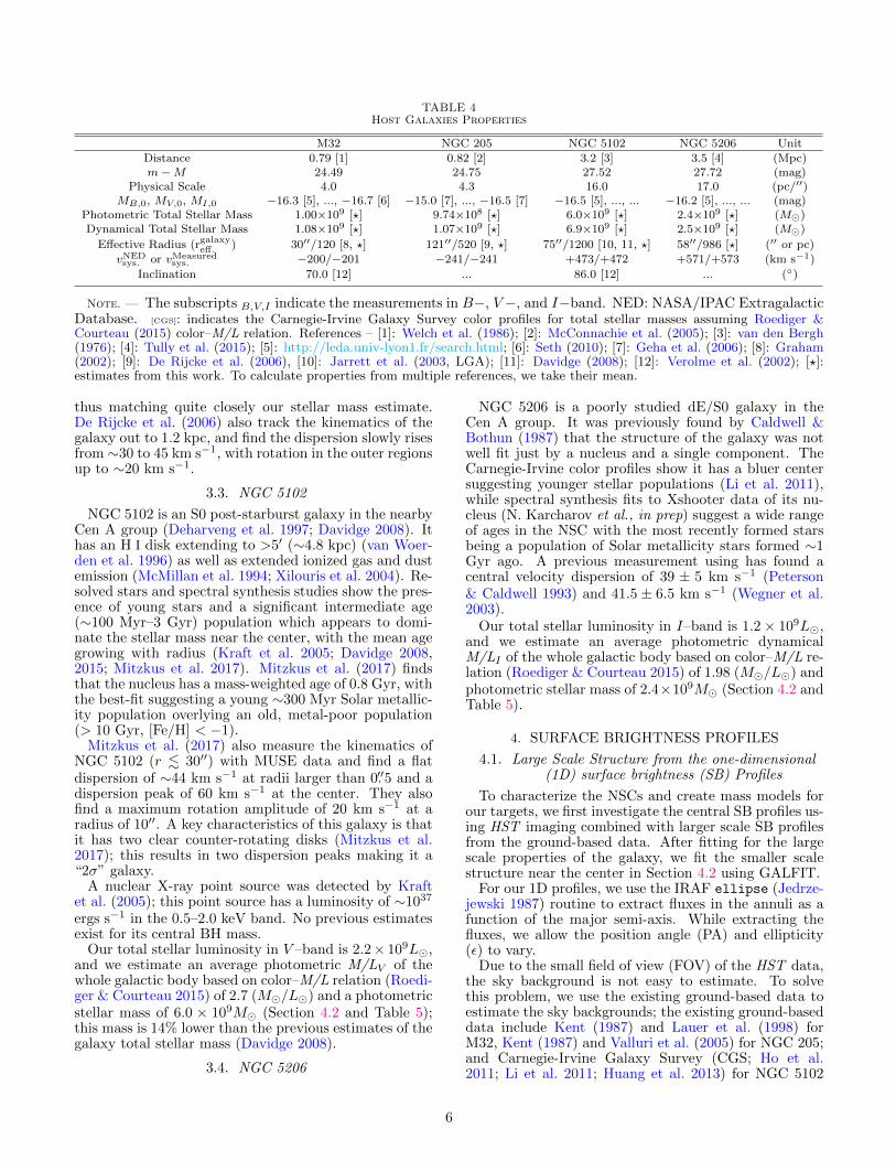
TABLE 4Host Galaxies Properties

M32 NGC 205 NGC 5102 NGC 5206 Unit

Distance 0.79 [1] 0.82 [2] 3.2 [3] 3.5 [4] (Mpc)m−M 24.49 24.75 27.52 27.72 (mag)

Physical Scale 4.0 4.3 16.0 17.0 (pc/′′)MB,0, MV,0, MI,0 −16.3 [5], ..., −16.7 [6] −15.0 [7], ..., −16.5 [7] −16.5 [5], ..., ... −16.2 [5], ..., ... (mag)

Photometric Total Stellar Mass 1.00×109 [?] 9.74×108 [?] 6.0×109 [?] 2.4×109 [?] (M�)Dynamical Total Stellar Mass 1.08×109 [?] 1.07×109 [?] 6.9×109 [?] 2.5×109 [?] (M�)

Effective Radius (rgalaxyeff. ) 30′′/120 [8, ?] 121′′/520 [9, ?] 75′′/1200 [10, 11, ?] 58′′/986 [?] (′′ or pc)

vNEDsys. or vMeasured

sys. −200/−201 −241/−241 +473/+472 +571/+573 (km s−1)

Inclination 70.0 [12] ... 86.0 [12] ... (◦)

Note. — The subscripts B,V,I indicate the measurements in B−, V−, and I−band. NED: NASA/IPAC ExtragalacticDatabase. [CGS]: indicates the Carnegie-Irvine Galaxy Survey color profiles for total stellar masses assuming Roediger &Courteau (2015) color–M/L relation. References – [1]: Welch et al. (1986); [2]: McConnachie et al. (2005); [3]: van den Bergh(1976); [4]: Tully et al. (2015); [5]: http://leda.univ-lyon1.fr/search.html; [6]: Seth (2010); [7]: Geha et al. (2006); [8]: Graham(2002); [9]: De Rijcke et al. (2006), [10]: Jarrett et al. (2003, LGA); [11]: Davidge (2008); [12]: Verolme et al. (2002); [?]:estimates from this work. To calculate properties from multiple references, we take their mean.

thus matching quite closely our stellar mass estimate.De Rijcke et al. (2006) also track the kinematics of thegalaxy out to 1.2 kpc, and find the dispersion slowly risesfrom ∼30 to 45 km s−1, with rotation in the outer regionsup to ∼20 km s−1.

3.3. NGC 5102

NGC 5102 is an S0 post-starburst galaxy in the nearbyCen A group (Deharveng et al. 1997; Davidge 2008). Ithas an H I disk extending to >5′ (∼4.8 kpc) (van Woer-den et al. 1996) as well as extended ionized gas and dustemission (McMillan et al. 1994; Xilouris et al. 2004). Re-solved stars and spectral synthesis studies show the pres-ence of young stars and a significant intermediate age(∼100 Myr–3 Gyr) population which appears to domi-nate the stellar mass near the center, with the mean agegrowing with radius (Kraft et al. 2005; Davidge 2008,2015; Mitzkus et al. 2017). Mitzkus et al. (2017) findsthat the nucleus has a mass-weighted age of 0.8 Gyr, withthe best-fit suggesting a young ∼300 Myr Solar metallic-ity population overlying an old, metal-poor population(> 10 Gyr, [Fe/H] < −1).

Mitzkus et al. (2017) also measure the kinematics ofNGC 5102 (r . 30′′) with MUSE data and find a flatdispersion of ∼44 km s−1 at radii larger than 0.′′5 and adispersion peak of 60 km s−1 at the center. They alsofind a maximum rotation amplitude of 20 km s−1 at aradius of 10′′. A key characteristics of this galaxy is thatit has two clear counter-rotating disks (Mitzkus et al.2017); this results in two dispersion peaks making it a“2σ” galaxy.

A nuclear X-ray point source was detected by Kraftet al. (2005); this point source has a luminosity of ∼1037

ergs s−1 in the 0.5–2.0 keV band. No previous estimatesexist for its central BH mass.

Our total stellar luminosity in V –band is 2.2× 109L�,and we estimate an average photometric M/LV of thewhole galactic body based on color–M/L relation (Roedi-ger & Courteau 2015) of 2.7 (M�/L�) and a photometricstellar mass of 6.0 × 109M� (Section 4.2 and Table 5);this mass is 14% lower than the previous estimates of thegalaxy total stellar mass (Davidge 2008).

3.4. NGC 5206

NGC 5206 is a poorly studied dE/S0 galaxy in theCen A group. It was previously found by Caldwell &Bothun (1987) that the structure of the galaxy was notwell fit just by a nucleus and a single component. TheCarnegie-Irvine color profiles show it has a bluer centersuggesting younger stellar populations (Li et al. 2011),while spectral synthesis fits to Xshooter data of its nu-cleus (N. Karcharov et al., in prep) suggest a wide rangeof ages in the NSC with the most recently formed starsbeing a population of Solar metallicity stars formed ∼1Gyr ago. A previous measurement using has found acentral velocity dispersion of 39 ± 5 km s−1 (Peterson& Caldwell 1993) and 41.5 ± 6.5 km s−1 (Wegner et al.2003).

Our total stellar luminosity in I–band is 1.2× 109L�,and we estimate an average photometric dynamicalM/LI of the whole galactic body based on color–M/L re-lation (Roediger & Courteau 2015) of 1.98 (M�/L�) andphotometric stellar mass of 2.4×109M� (Section 4.2 andTable 5).

4. SURFACE BRIGHTNESS PROFILES

4.1. Large Scale Structure from the one-dimensional(1D) surface brightness (SB) Profiles

To characterize the NSCs and create mass models forour targets, we first investigate the central SB profiles us-ing HST imaging combined with larger scale SB profilesfrom the ground-based data. After fitting for the largescale properties of the galaxy, we fit the smaller scalestructure near the center in Section 4.2 using GALFIT.

For our 1D profiles, we use the IRAF ellipse (Jedrze-jewski 1987) routine to extract fluxes in the annuli as afunction of the major semi-axis. While extracting thefluxes, we allow the position angle (PA) and ellipticity(ε) to vary.

Due to the small field of view (FOV) of the HST data,the sky background is not easy to estimate. To solvethis problem, we use the existing ground-based data toestimate the sky backgrounds; the existing ground-baseddata include Kent (1987) and Lauer et al. (1998) forM32, Kent (1987) and Valluri et al. (2005) for NGC 205;and Carnegie-Irvine Galaxy Survey (CGS; Ho et al.2011; Li et al. 2011; Huang et al. 2013) for NGC 5102

6

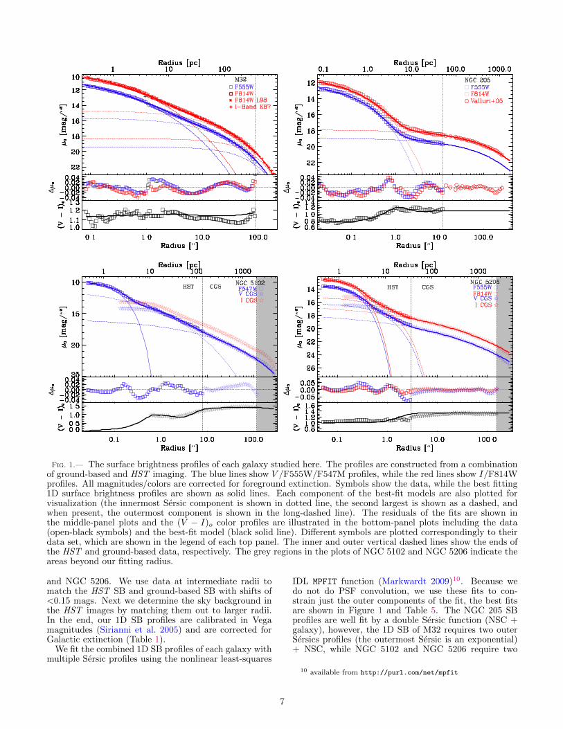
Fig. 1.— The surface brightness profiles of each galaxy studied here. The profiles are constructed from a combinationof ground-based and HST imaging. The blue lines show V /F555W/F547M profiles, while the red lines show I/F814Wprofiles. All magnitudes/colors are corrected for foreground extinction. Symbols show the data, while the best fitting1D surface brightness profiles are shown as solid lines. Each component of the best-fit models are also plotted forvisualization (the innermost Sersic component is shown in dotted line, the second largest is shown as a dashed, andwhen present, the outermost component is shown in the long-dashed line). The residuals of the fits are shown inthe middle-panel plots and the (V − I)o color profiles are illustrated in the bottom-panel plots including the data(open-black symbols) and the best-fit model (black solid line). Different symbols are plotted correspondingly to theirdata set, which are shown in the legend of each top panel. The inner and outer vertical dashed lines show the ends ofthe HST and ground-based data, respectively. The grey regions in the plots of NGC 5102 and NGC 5206 indicate theareas beyond our fitting radius.

and NGC 5206. We use data at intermediate radii tomatch the HST SB and ground-based SB with shifts of<0.15 mags. Next we determine the sky background inthe HST images by matching them out to larger radii.In the end, our 1D SB profiles are calibrated in Vegamagnitudes (Sirianni et al. 2005) and are corrected forGalactic extinction (Table 1).

We fit the combined 1D SB profiles of each galaxy withmultiple Sersic profiles using the nonlinear least-squares

IDL MPFIT function (Markwardt 2009)10. Because wedo not do PSF convolution, we use these fits to con-strain just the outer components of the fit, the best fitsare shown in Figure 1 and Table 5. The NGC 205 SBprofiles are well fit by a double Sersic function (NSC +galaxy), however, the 1D SB of M32 requires two outerSersics profiles (the outermost Sersic is an exponential)+ NSC, while NGC 5102 and NGC 5206 require two

10 available from http://purl.com/net/mpfit

7

NSC Sersic components + a galaxy component based ontheir 2D fits. We note that our exponential disk compo-nent of M32 and the outer Sersis component of NGC 205are fully consistent with Graham (2002) and Graham &Spitler (2009), and these components will be fixed in 2DGALFIT (Section 4.2). The robustness of our 1D fits aretested by changing the outer boundaries in the ranges of70′′–90′′, 100′′–200′′, 90′′–110′′, and 90′′–120′′ for M32,NGC 205, NGC 5102, and NGC 5206, respectively. Thestandard deviation of the Sersic parameters from thesefits was used to determine the errors; these errors are<10% in all cases. The fits are performed in multiplebands, enabling us to model the color variation.

We show the 1D SB profile fits, residuals, and (V −I)o

color of each galaxy in the top- middle-, and bottom-panel of each plot in Figure 1. These models agree wellwithin the data with MEAN(ABS((data-model)/data)<5% for all four galaxies. M32 shows no radial colorgradient, consistent with previous observations (Laueret al. 1998). The other three galaxies show bluer colorstoward their centers. We also note that we use thesemodels only to constrain the outer Sersic components ofthe galaxies, the best-fit inner components are derivedfrom 2D modeling of the HST images.

4.2. NSC morphology from 2D GALFIT Models

Our dynamical models rely on the accurate measure-ments of the 2D stellar mass distribution near the centersof each galaxy. Moreover, the 2D SB profile is also im-portant for quantifying the morphology of the NSCs. Wemodel the HST images around the nucleus using GAL-FIT. GALFIT enables fitting with convolved models (us-ing a PSF from Tiny Tim, Section 2.3), and excludingpixels using a bad pixel mask. The bad pixel mask isobtained using an initial GALFIT run without a mask;we mask all pixels with absolute pixel values >3σ thanthe median value in the residual images (Data-Model).Based on our 1D SB profile, we chose to fit NGC 205with a double-Sersic function (2S), M32 is fitted witha 2S + Exponential disk (2S + E). For NGC 5102 andNGC 5206 we find the nuclear regions require two com-ponents (Figure 2), and thus these are fitted with triple-Sersic functions (3S). The initial guesses were input withthe best-fit parameters from the 1D SB fits with fixed pa-rameters for the outermost Sersic or E component exceptfor the PA and axis ratio (b/a). For the purpose of cre-ating mass models for dynamical modeling of BH massesmeasurements, we repeat these 2D fit with fixed PA in allSersic components because the Jeans Anisotropic Mod-els (JAM; Cappellari 2008) assume axisymmetry, whichimplies a constant PA.

The left column of Figure 2 show the F814W imagesof M32, NGC 205, and NGC 5206 and F547M imageof NGC 5102, while the middle column show their rela-tive errors between the HST images and their 2S mod-els, (Data-Model)/Data. The right column also showthese relative errors between the HST images and their2S + E (M32) or 3S (NGC 5102 and NGC 5206) models.The contours on each panel show both data (black) andmodel (white) at the same radius and flux level to high-light the regions of agreement and disagreement betweendata and models. Excluding masked regions (and pointsources in NGC 205), the maximum errors on the individ-ual fits are <9%, 15%, 13%, and 10% for M32, NGC 205,

NGC 5102, and NGC 5206, respectively. The parametersof the best-fit GALFIT models are shown in Columns 4–9 of Table 5; errors are scaled based on the 1D errorsin the components estimated in Section 4.1 due to theirdominant over the GALFIT errors. We note that the2D GALFIT models give Sersic parameters consistent tothat of 1D SB profiles fit, especially for the middle Sersiccomponents where the PSF effects are minimal. We notethat our NSC component in M32 is significantly less lu-minous than the 1D SB profile given in Graham & Spitler(2009); we believe this is at least in part due to their nor-malization in the SB profile, which is nearly a magnitudehigher than that derived here.

Next, we use the final fixed-PA 2D GALFIT Sersicmodels to create multi-Gaussian expansion (MGEs; Em-sellem et al. 1994a,b; Cappellari & Emsellem 2004) mod-els. These MGEs are comprised of a total of 18, 10, 14,and 14 Gaussians to provide a satisfactory fit to the sur-face mass density profiles of M32, NGC 205, NGC 5102,and NGC 5206 respectively. We fit our MGEs out to∼110.′′0 for M32 and NGC 5206, 15.′′0 for NGC 205, 21.′′0for NGC 5102 and obtain the mass models by straight-forward multiplying the M/L profiles with the 2D lightGALFIT MGEs at the corresponding radii. We chooseto parameterize the mass models using GALFIT (asopposed to using the fit sectors mge code) because(1) it enables us to properly incorporate the complexHST PSF, and (2) it enables simple separation of NSCand galaxy components.

4.3. Color–M/L Relations

To turn our stellar luminosity profiles into stellar massprofiles, we assume a M/L–color relation. There is astrong correlation between the color and the M/L of astellar population: we use two different color–M/L re-lations including the Bell et al. (2003) (hereafter B03),Roediger & Courteau (2015) (henceforth R15) color–M/L correlations, as well as models with constant M/L.This is similar to the method presented by Nguyen et al.(2017) for analysis of the NGC 404 nucleus. For our best-fit models we use the R15 relation, which was found byNguyen et al. (2017) to be within 1σ of the color–M/L re-lation derived from stellar population fits to STIS datawithin the nucleus. The B03 and constant M/L mod-els are used to assess the systematic uncertainties in ourmass models. The B03 and R15 relations are built basedon the (V −I)0 color profiles in the bottom panel of eachplot in Figure 1, except in NGC 5102. For NGC 5102,we use the (B − V )0 color estimated from the combinedHST F547M–F656N data at small radii and F450W–F569W data at larger radii as described in the appendixA.

We also create mass models with a constant centralM/L. For these models, we take a reasonable referencevalue for the M/L, but still allow these values to bescaled in our dynamical models, just as for the varyingM/L models. We note that these models are not used inany of our final results, but are used to analyze poten-tial systematic errors in our dynamical modeling. Thereference values used for the constant M/L models are:

• M32: We use M/LI = 1.41 (M�/L�) based onthe Schwarzschild model fits to Sauron data fromCappellari et al. (2006).

8

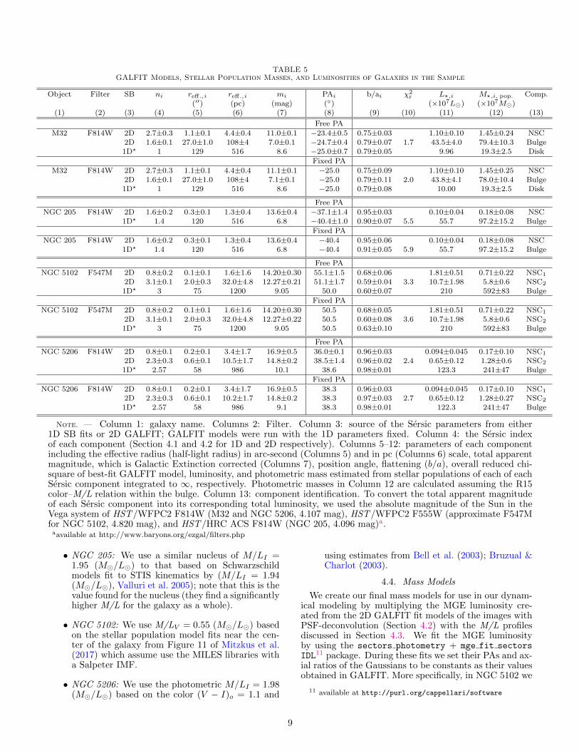
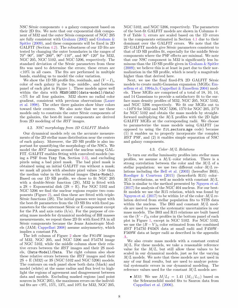
TABLE 5GALFIT Models, Stellar Population Masses, and Luminosities of Galaxies in the Sample

Object Filter SB ni reff.,i reff.,i mi PAi b/ai χ2r L?,i M?,i, pop. Comp.

(′′) (pc) (mag) (◦) (×107L�) (×107M�)(1) (2) (3) (4) (5) (6) (7) (8) (9) (10) (11) (12) (13)

Free PA

M32 F814W 2D 2.7±0.3 1.1±0.1 4.4±0.4 11.0±0.1 −23.4±0.5 0.75±0.03 1.10±0.10 1.45±0.24 NSC2D 1.6±0.1 27.0±1.0 108±4 7.0±0.1 −24.7±0.4 0.79±0.07 1.7 43.5±4.0 79.4±10.3 Bulge1D? 1 129 516 8.6 −25.0±0.7 0.79±0.05 9.96 19.3±2.5 Disk

Fixed PA

M32 F814W 2D 2.7±0.3 1.1±0.1 4.4±0.4 11.1±0.1 −25.0 0.75±0.09 1.10±0.10 1.45±0.25 NSC2D 1.6±0.1 27.0±1.0 108±4 7.1±0.1 −25.0 0.79±0.11 2.0 43.8±4.1 78.0±10.4 Bulge1D? 1 129 516 8.6 −25.0 0.79±0.08 10.00 19.3±2.5 Disk

Free PA

NGC 205 F814W 2D 1.6±0.2 0.3±0.1 1.3±0.4 13.6±0.4 −37.1±1.4 0.95±0.03 0.10±0.04 0.18±0.08 NSC1D? 1.4 120 516 6.8 −40.4±1.0 0.90±0.07 5.5 55.7 97.2±15.2 Bulge

Fixed PA

NGC 205 F814W 2D 1.6±0.2 0.3±0.1 1.3±0.4 13.6±0.4 −40.4 0.95±0.06 0.10±0.04 0.18±0.08 NSC1D? 1.4 120 516 6.8 −40.4 0.91±0.05 5.9 55.7 97.2±15.2 Bulge

Free PA

NGC 5102 F547M 2D 0.8±0.2 0.1±0.1 1.6±1.6 14.20±0.30 55.1±1.5 0.68±0.06 1.81±0.51 0.71±0.22 NSC1

2D 3.1±0.1 2.0±0.3 32.0±4.8 12.27±0.21 51.1±1.7 0.59±0.04 3.3 10.7±1.98 5.8±0.6 NSC2

1D? 3 75 1200 9.05 50.0 0.60±0.07 210 592±83 Bulge

Fixed PA

NGC 5102 F547M 2D 0.8±0.2 0.1±0.1 1.6±1.6 14.20±0.30 50.5 0.68±0.05 1.81±0.51 0.71±0.22 NSC1

2D 3.1±0.1 2.0±0.3 32.0±4.8 12.27±0.22 50.5 0.60±0.08 3.6 10.7±1.98 5.8±0.6 NSC2

1D? 3 75 1200 9.05 50.5 0.63±0.10 210 592±83 Bulge

Free PA

NGC 5206 F814W 2D 0.8±0.1 0.2±0.1 3.4±1.7 16.9±0.5 36.0±0.1 0.96±0.03 0.094±0.045 0.17±0.10 NSC1

2D 2.3±0.3 0.6±0.1 10.5±1.7 14.8±0.2 38.5±1.4 0.96±0.02 2.4 0.65±0.12 1.28±0.6 NSC2

1D? 2.57 58 986 10.1 38.6 0.98±0.01 123.3 241±47 Bulge

Fixed PA

NGC 5206 F814W 2D 0.8±0.1 0.2±0.1 3.4±1.7 16.9±0.5 38.3 0.96±0.03 0.094±0.045 0.17±0.10 NSC1

2D 2.3±0.3 0.6±0.1 10.2±1.7 14.8±0.2 38.3 0.97±0.03 2.7 0.65±0.12 1.28±0.27 NSC2

1D? 2.57 58 986 9.1 38.3 0.98±0.01 122.3 241±47 Bulge

Note. — Column 1: galaxy name. Columns 2: Filter. Column 3: source of the Sersic parameters from either1D SB fits or 2D GALFIT; GALFIT models were run with the 1D parameters fixed. Column 4: the Sersic indexof each component (Section 4.1 and 4.2 for 1D and 2D respectively). Columns 5–12: parameters of each componentincluding the effective radius (half-light radius) in arc-second (Columns 5) and in pc (Columns 6) scale, total apparentmagnitude, which is Galactic Extinction corrected (Columns 7), position angle, flattening (b/a), overall reduced chi-square of best-fit GALFIT model, luminosity, and photometric mass estimated from stellar populations of each of eachSersic component integrated to ∞, respectively. Photometric masses in Column 12 are calculated assuming the R15color–M/L relation within the bulge. Column 13: component identification. To convert the total apparent magnitudeof each Sersic component into its corresponding total luminosity, we used the absolute magnitude of the Sun in theVega system of HST/WFPC2 F814W (M32 and NGC 5206, 4.107 mag), HST/WFPC2 F555W (approximate F547Mfor NGC 5102, 4.820 mag), and HST/HRC ACS F814W (NGC 205, 4.096 mag)a.

aavailable at http://www.baryons.org/ezgal/filters.php

• NGC 205: We use a similar nucleus of M/LI =1.95 (M�/L�) to that based on Schwarzschildmodels fit to STIS kinematics by (M/LI = 1.94(M�/L�), Valluri et al. 2005); note that this is thevalue found for the nucleus (they find a significantlyhigher M/L for the galaxy as a whole).

• NGC 5102: We use M/LV = 0.55 (M�/L�) basedon the stellar population model fits near the cen-ter of the galaxy from Figure 11 of Mitzkus et al.(2017) which assume use the MILES libraries witha Salpeter IMF.

• NGC 5206: We use the photometric M/LI = 1.98(M�/L�) based on the color (V − I)o = 1.1 and

using estimates from Bell et al. (2003); Bruzual &Charlot (2003).

4.4. Mass Models

We create our final mass models for use in our dynam-ical modeling by multiplying the MGE luminosity cre-ated from the 2D GALFIT fit models of the images withPSF-deconvolution (Section 4.2) with the M/L profilesdiscussed in Section 4.3. We fit the MGE luminosityby using the sectors photometry + mge fit sectorsIDL11 package. During these fits we set their PAs and ax-ial ratios of the Gaussians to be constants as their valuesobtained in GALFIT. More specifically, in NGC 5102 we

11 available at http://purl.org/cappellari/software

9

Fig. 2.— Comparison of HST images to their GALFIT models for each galaxy. Left panels: the 2D HST/WFPC2PC (M32, NGC 5102, NGC 5206) or ACS/HRC (NGC 205) images. Middle panels: the fractional residual(Data-Model)/Data between the HST imaging and their corresponding two-component GALFIT models. Rightpanels: fractional residuals from the three-components GALFIT models. The data and model contours are shown atthe same levels of flux and radius in black and white repeating from the left to the right panels, respectively. Allfigures show East to the left, and North up.

10

0.01 0.10 1.00 10.00 100.00Radius ["]102

103

104

105

106

107

Σ [

MO • p

c-2]

0.1 1.0 10.0 100.0 1000.0Radius [pc]

F814WM32

R15B03M/L = 1.41NSC

F814WM32

0.01 0.10 1.00 10.00 100.00Radius ["]

-20-10

0

10

20

Dif

f [%

] +10%

-10%

0.1 1.0 10.0 100.0Radius ["]

103

104

105

Σ [

MO • p

c-2]

0.1 1.0 10.0 100.0Radius [pc]

R15B03M/L = 1.95NSC

F814WNGC 205

0.1 1.0 10.0 100.0Radius ["]

-20-10

0

10

20

Dif

f [%

]

-10%

+10%

0.1 1.0 10.0 100.0Radius ["]102

103

104

105

106

Σ [

MO • p

c-2]

1 10 100 1000Radius [pc]

R15B03M/L = 0.55NSC

F547MNGC 5102

0.1 1.0 10.0 100.0Radius ["]

-20

-10

0

10

20

Dif

f [%

] +10%

-10%

0.1 1.0 10.0 100.0Radius ["]102

103

104

105

Σ [

MO • p

c-2]

10 100 1000Radius [pc]

R15B03M/L = 1.98NSC

F814WNGC 5206

0.1 1.0 10.0 100.0Radius ["]

-20-10

0

10

20

Dif

f [%

] +10%

-10%

Fig. 3.— Top panels: Comparison of the mass surface density models in each galaxy. These models are createdusing MGEs constructed from our GALFIT models. These MGEs are then multiplied by a M/L to get a mass surfacedensity. For the constant M/L model (dark blue) the chosen M/L is discussed in Section 4.3. For the other massmodels, an M/L is assigned to each MGE based on the color of the galaxy at the radius of the MGE using the R15or B03 color–M/L relation (red/purple lines); we use the R15 model as our default. Dashed black lines show theNSCs in the R15 model; their effective radii are shown by vertical lines. Bottom panels: To compare the relative massdistribution of the three different mass profiles for each galaxy, we plot their fractional difference relative to the R15color–M/L relation.

Fig. 4.— Left panel: The radial velocity map derived from CO bandhead spectroscopy from Gemini/NIFS of NGC 205before central resolved stars subtraction. The white intensity contours are plotted overlay on top of the map showthose resolved star in the FOV with the two brights on north-west (purple plus) and south-west (red plus) of the map.Middle panel: The spectrum of the brightest purple plus star is shown in the same color respectively. Right panel: Theradial velocity map derived from CO bandhead spectroscopy from Gemini/NIFS of NGC 205 after central resolvedstar subtraction (Section 5.2). The white intensity contours after the subtraction of resolved stars are now smoother.

calculate the V –band M/L and apply this to the F547Mdata, while in the others, we calculate I–band M/Ls andapply these to the F814W data.

The top-panel in each plot of Figure 3 shows the masssurface density and the bottom-panel shows the rela-tive error of the M/L profile relative to the R15 color–M/L correlation for each galaxy. It is clear that the R15color–M/L correlation (red line) predicts less mass at thecenter of each galaxy than the prediction of B03 color–M/L correlation (purple line). However, the assumptionof constant M/Ls (blue line) predict more mass at thecenters but less mass at larger radii than the predictionsof both B03 and R15 color–M/L correlation. This is asexpected based on the bluer centers and consequentlylower M/Ls at the centers. The MGEs of mass surfacedensities of M32, NGC 205, NGC 5102, and NGC 5206

are presented in column (2) of Table B4 (Appendix B).

4.5. K–Band Luminosities

Together with the stellar mass distribution, the dy-namical models also require as input the distribution ofthe stellar tracer population from which the kinemat-ics is obtained. Given that the kinematics was derivedin the K–band, which covers the wavelengths from 2.29to 2.34µm, we create high-resolution synthetic imagesin that band (Ahn et al. 2017). We do not use theK–band images obtained from the IFU observations di-rectly as they have lower resolution and too limited FOV.To make these we employ Padova SSP model (Bressanet al. 2012) to fit color–color correlations. The pur-pose of this is to transform our HST imaging of F555Wand F814W (of M32, NGC 205, and NGC 5206) into

11

0.1 0.2 0.3 0.4 0.5 0.6 0.7Radius ["]

202530354045

VR

MS [

km

s−

1]

2. 4. 6. 8. 10.Radius [pc]

NGC 5206

0.0 0.1 0.2 0.3 0.4 0.5 0.6 0.7Radius ["]

010203040

Vel

oci

ty

VROT

σ

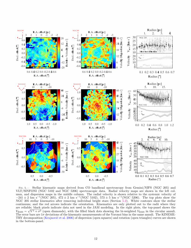
Fig. 5.— Stellar kinematic maps derived from CO bandhead spectroscopy from Gemini/NIFS (NGC 205) andVLT/SINFONI (NGC 5102 and NGC 5206) spectroscopic data. Radial velocity maps are shown in the left col-umn, and dispersion maps in the middle column. The radial velocity is shown relative to the systemic velocity of−241 ± 2 km s−1(NGC 205), 472 ± 2 km s−1(NGC 5102), 573 ± 5 km s−1(NGC 5206). The top plots show theNGC 205 stellar kinematics after removing individual bright stars (Section 5.2). White contours show the stellarcontinuum; and the red arrows indicate the orientation. Kinematics are only plotted out to the radii where theyare reliable; black pixels indicate data not used in the JAM modeling. In the right plots, the top-panel shows theVRMS =

√V 2 + σ2 (open diamonds), with the filled black dots showing the bi-weighted VRMS in the circular annuli.

The error bars are 1σ deviations of the kinematic measurements of the Voronoi bins in the same annuli. The KINEME-TRY decomposition (Krajnovic et al. 2006) of dispersion (open squares) and rotation (open triangles) curves are shownin the bottom-panel.

12

K–band images. Specifically, we fit the linear correla-tions of HST F555W–F814W vs. F814W–K based onthe specific nucleus stellar populations and metallicitiesfor M32 (Z = 0.019, Corbin et al. 2001), NGC 205(Z = 0.008, Butler & Martınez-Delgado 2005), andNGC 5206 (Z = 0.004 − 0.008; N. Kacharov et al., inprep.). We use these to create K–band images basedon the reference HST images (i.e., we add the color cor-rection to the F814W image). These K band imagesare similar to the I–band images, with deviations in theSB profile being comparable to differences between massmodels shown in Figure 3.

In order to create a K–band image for NGC 5102, weuse its F450W–F569W colors, which are inferred fromthe F547M–F656N data as described in the appendix A.Next, we fit a linear correlation of HST F450W–F569Wvs. F569W–K using metallicities Z = 0.004 (Davidge2015), then infer for its K–band images. We then fitthe MGEs using the mge fit sectors IDL12 package.The MGEs K–band luminosity surface densities of M32,NGC 205, NGC 5102, and NGC 5206 are given in column(1) Table B4 (Appendix B).

5. STELLAR KINEMATICS RESULTS

We use adaptive optics NIFS and SINFONI spec-troscopy to determine the nuclear stellar kinematics in allfour galaxies. We first re-bin spatial pixels within eachwavelength of the data cube using the Voronoi binningmethod (Cappellari & Copin 2003) to obtain S/N & 25per spectral pixel. Next, we use the pPXF method (Cap-pellari & Emsellem 2004; Cappellari 2017) to derive thestellar kinematics from the CO band-heads of the NIFSand SINFONI spectroscopy in the wavelength range of2.280–2.395 µm and determine the line-of-sight velocitydistribution (LOSVD). We fit only a Gaussian LOSVD,measuring the radial velocity (V ) and dispersion (σ) us-ing high spectral resolution of stellar templates of eightsupergiant, giant, and main-sequence stars with spectraltypes between G and M with all luminosity classes (Wal-lace & Hinkle 1996). These templates are matched to theresolution of the observations by convolving them by aGaussian with dispersion equal to that of the line-spreadfunction (LSF) of the observed spectra at every wave-length. These LSFs are determined from sky lines. ForNIFS, the LSF is quite Gaussian with a FWHM ∼4.2 A,but the width varies across the FOV (e.g., Seth 2010).However, the SINFONI LSF appears to be significantlynon-Gaussian as seen from the shape of the OH sky lines.To characterize the shape of the LSF and its potentialvariation across the FOV, we reduced the sky frames inthe same way as the science frames, with the differencethat we did not subtract the sky. We then combined thereduced sky cubes using the same dither pattern as thescience frames. This ensured that the measured LSF onthe resulting sky lines fully resembles the one on the ob-ject lines. From these dithered sky lines we measured theLSF. We used 6 isolated, strong sky lines, all having closedoublets, except one (the 21,995 A line), to measure thespectral resolution across the detector. Since the LSFappears to be constant along rows (constant y values),the sky cubes were collapsed along the y-direction.


Sky emissions OH-lines can be described as a deltafunction, δλ. Once they reach the spectrograph they willbe dispersed so that the intensity pattern is redistributedwith wavelength according to the LSF of the instrument.Since we know the central wavelength of the sky emis-sion lines we assume that their shapes represent the LSF.Once located, the peak values in the spectra and a regionaround the peaks is defined, the continuum is subtracted,the line flux is normalized to the peak flux and finally thelines are summed up.

The spectral resolution across the detector has a me-dian value of 6.32 A FWHM ( λ

∆λ = 3820) with values

ranging from 5.46 to 6.7 A FWHM (R ∼ 3440 – 4300).The last step before the kinematic extraction is to per-form the same binning on the LSF cube as for the sciencecube. This varying LSF is then used in the kinematic ex-traction with pPXF.

To obtain optimal kinematics from the SINFONI datawe had to correct for several effects: (1) a scattered lightcomponent and (2) velocity differences between individ-ual cubes. For the first issue, the SINFONI data cubeshave imperfect sky subtraction, with clear additive resid-uals remaining despite subtraction of sky cubes. Theseresiduals appear to have a uniform spectrum that is spa-tially constant across the field, however the residuals arenot clearly identified as sky or stellar spectra. To removethese residuals, we create a median residual spectrum foreach individual data cube using pixels beyond 1.′′3 radiusand subtract it from all spaxels in the cube. This sub-traction greatly improved the quality of our kinematicfits to our final combined data cube, but we note thatthis is likely also subtracting some galaxy light from eachpixel. Second, fits to sky lines revealed variations in thewavelength solutions corresponding to velocity offsets ofup to 20 km s−1 between individual data cubes. There-fore before combining the cubes, we applied a velocityshift to correct these shifts; 4/12 cubes for NGC 5102 and3/12 cubes for NGC 5206 were shifted before combiningbringing the radial velocity errors .2 km s−1 among thecubes to their means for both galaxies. We note howeverthat applying these velocity shifts had minimal impact(<0.5 km s−1) on the derived dispersions. The systemicvelocity in each galaxy was estimated by taking a medianof pixels with radii <0.′′15, and is listed in Table 4.

To calculate the errors on the LOSVD, we add Gaus-sian random errors to each spectral pixel and applyMonte Carlo simulations to re-run the pPXF code. Theerrors used differ in NIFS and SINFONI; for NIFS wehave an error spectrum available, and these are usedto run the Monte Carlo, while with SINFONI, no errorspectrum is available, and we therefore use the standarddeviation of the pPXF fit residuals as a uniform erroron each pixel. We test further the robustness of ourkinematic results by (1) fitting the spectra toward theshort wavelength range 2.280–2.338 µm of the CO band-heads (the highest S/N portion of the CO bandhead) and(2) using the PHOENIX model spectra (Husser et al.2013), which have higher resolution (R = 500, 000 or 0.6km s−1) than the Wallace & Hinkle (1996) (R = 45, 000or 6.67 km s−1) templates. We find consistent kinematicresults within the errors with (1) returning dispersions1–2 km s−1 higher than the full spectral range, while (2)yields fully consistent results. We also verified our SIN-

13

106

MBH [MO •]

-0.6

-0.4

-0.2

0.0

0.2

βz

106

-0.6

-0.4

-0.2

0.0

0.2

106

-0.6

-0.4

-0.2

0.0

0.2M32R15B03

Const.

106

MBH [MO •]

0.8

0.9

1.0

1.1

1.2

1.3

(M/L dyn./M/L pop.)F814W

106

0.8

0.9

1.0

1.1

1.2

1.3

(M/L

dyn./M

/L p

op.) F

814W

106

0.8

0.9

1.0

1.1

1.2

1.3

M32R15B03

Const.

106

MBH [MO •]

65

70

75

80

i [°

]

106

106

65

70

75

80

65

70

75

80

M32R15B03

Const.

105

MBH [MO •]

0.15

0.20

0.25

0.30

0.35

βz

105

0.15

0.20

0.25

0.30

0.35

105

0.15

0.20

0.25

0.30

0.35NGC 205 (After Star Subtraction)

R15B03

Const.

105MBH [MO •]

0.95

1.00

1.05

1.10

1.15

1.20

(M/L dyn./M/L pop.)F814W

105

MBH [MO •]

0.95

1.00

1.05

1.10

1.15

1.20

(M/L

dyn./M

/L p

op.) F

814W

105

0.95

1.00

1.05

1.10

1.15

1.20NGC 205 (After Star Subtraction)R15B03

Const.

105MBH [MO •]50

55

60

65

70

i [°]

105

MBH [MO •]

105

50

55

60

65

70

i [°

]

50

55

60

65

70

NGC 205 (After Star Subtraction)R15B03

Const.

105 106

MBH [MO •]

0.0

0.1

0.2

0.3

βz

105 106

0.0

0.1

0.2

0.3

105 106

0.0

0.1

0.2

0.3

NGC 5102Const.B03R15

105 106

MBH [MO •]

1.10

1.15

1.20

(M/L

dyn./M

/L p

op.) F

547M

105 106

1.10

1.15

1.20

105 106

1.10

1.15

1.20


105 106

MBH [MO •]

65

70

75

80

85

i [°

]

105 106

105 106

65

70

75

80

85

65

70

75

80

85


104 105 106

MBH [MO •]

0.10

0.15

0.20

0.25

0.30

0.35

βz

104 105 106

0.10

0.15

0.20

0.25

0.30

0.35

104 105 106

0.10

0.15

0.20

0.25

0.30

0.35


104 105 106

MBH [MO •]

0.8

0.9

1.0

1.1

1.2

1.3

(M/L

dyn./M

/Lpop.) F

814W

104 105 106

0.8

0.9

1.0

1.1

1.2

1.3

104 105 106

0.8

0.9

1.0

1.1

1.2

1.3


104 105 106

MBH [MO •]

40

45

50

55

i [°

]

104 105 106

104 105 106

40

45

50

55

40

45

50

55


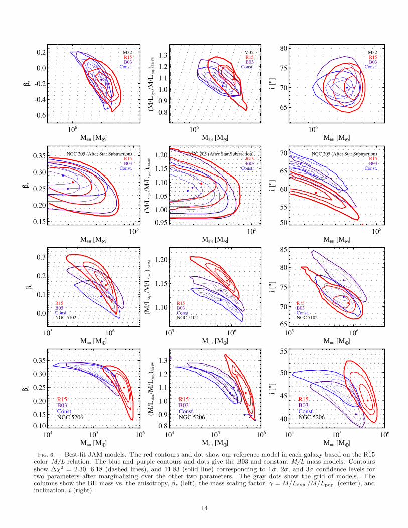
Fig. 6.— Best-fit JAM models. The red contours and dot show our reference model in each galaxy based on the R15color–M/L relation. The blue and purple contours and dots give the B03 and constant M/L mass models. Contoursshow ∆χ2 = 2.30, 6.18 (dashed lines), and 11.83 (solid line) corresponding to 1σ, 2σ, and 3σ confidence levels fortwo parameters after marginalizing over the other two parameters. The gray dots show the grid of models. Thecolumns show the BH mass vs. the anisotropy, βz (left), the mass scaling factor, γ = M/Ldyn./M/Lpop. (center), andinclination, i (right).

14

FONI kinematic errors by combining independent sub-sets of the data and identical binning and found thattheir distribution had a scatter similar to the error; asimilar verification of the NIFS errors was done in Sethet al. (2014). This analysis indicates that the radial ve-locities and dispersion errors range from 0.5–20 km s−1.These kinematic data are presented in Table B1, B2, andB3 for NGC 205, NGC 5102, and NGC 5206 respectivelyin the appendix B, except for M32, which was publishedin Table 1 of Seth (2010).

Due to increased systematic errors affecting our kine-matic measurements at low surface brightness (wheremany pixels are binned together), we eliminate the out-ermost bins beyond an ellipse with semi-major axes of1.′′3, 1.′′2, 0.′′7, and 0.′′7 in M32, NGC 5102, NGC 5206,and NGC 205. In general, we find that in the noisydata in outer regions we overestimate our VRMS values.For instance in the M32 data published in Seth (2010),we find a rise in VRMS beyond 1.′′3, however comparisonwith data from Verolme et al. (2002) suggests this risemay be due to systematic error, and is not used in theremainder of our analysis. In addition, we only plot andfit bins with dispersion and velocity errors <15 km s−1.We correct the systemic velocities (then radial velocities)for the barycentric correction (37 km s−1, 20 km s−1,−20 km s−1, and −37 km s−1 for M32, NGC 205,NGC 5102, and NGC 5206). The systemic velocitiesare determined from the central velocity as referencesand double checked with using the fit kinematic paIDL package13.

The final kinematic maps for NGC 205, NGC 5102 andNGC 5206 are shown in Figure 5. The left column showsthe radial velocity maps, the middle column shows thevelocity dispersion maps. The right most column showsthe VRMS measurements (open gray diamonds with errorbars, top panel) and the bi-weighted in the circular annuli(fill black dots with error bars). The bottom panel ofthe right column shows the results of KINEMETRY fits(Krajnovic et al. 2006), which determines the best-fitrotation and dispersion profiles along ellipses. We discussthe kinematics for each galaxy below.

5.1. M32

The kinematics of M32 were derived with pPXF us-ing a four-order of Gauss–Hermite series including V , σ,skewness (h3), and kurtosis (h4) (Seth 2010). These mea-surements are the highest quality kinematic data avail-able that resolve the sphere-of-influence (SOI) of the BH.These kinematics show a very clear signature of a rotat-ing and disky elliptical galaxy with strong rotation at aPA of−25◦ (E of N) with an amplitude of∼55 km s−1 be-yond the radius of 0.′′3 with the maximum of V/σ reach-ing 0.76 at r = 0.′′5 (2 pc). The dispersion has a peak of∼120 km s−1, which we will show is due to the influenceof the BH, and flattens out at ∼76 km s−1 beyond 0.′′5.

5.2. NGC 205

Of the nuclei considered here, NGC 205 is by far theone most dominated by individual stars. These areclearly visible in the HST images (Figure 2), and theireffects can be seen in our kinematics maps. These maps


show bright individual stars that often have decreaseddispersion and larger offsets from the systemic velocity,and therefore we have attempted to remove them beforederiving the kinematics as done in Kamann et al. (2013).The spectrum of the star weighted by the PSF was sub-tracted from all adjacent spectra of the cube. We sum-marize this process briefly here. First, we identify brightstars in the FOV of NIFS data manually by-eye and notedown their approximate spaxel coordinates in all layersof the data cube; there are 32 of these identified brightstars in total. Second, we estimate PSFs for these starsthat are well-described analytically either by Moffat ordouble-Gaussian; the differences between these two PSFrepresentations are small, but we use the Moffat pro-file in our final analysis. Next, we perform a combinedPSF fit for all identified stars; in this analysis, we modelthe contribution from the galaxy core as an additionalcomponent that is smoothly varying spatially. Third, weobtain spectra for all identified stars so that their infor-mation were used to subtract off from each layer of thecube. Finally, we use this star-subtracted cube to deter-mine the kinematics of underlying background light ofthe galaxy.

We show our original map of relative velocity in the leftpanel of Figure 4. One of the subtracted stellar spectrais shown in the middle panel, while velocity map afterthe stellar subtraction is shown in the right panel. Sub-traction of stars yields a much smoother velocity mapand isophotal contours than our original map. The com-plete kinematic maps determined after star subtractionare shown in the top row plots of Figure 5. We use thismap for all further analysis, but also include the originalmap in tests on the robustness of our results.

We examine the stellar rotational velocity (V ) and dis-persion velocity (σ?) of NGC 205. The dispersion ve-locity drops to ∼15 km s−1 within the 0.′′2 radius andreaches ∼23 km s−1 in the outer annulus of 0.′′2–0.′′8.This dispersion velocity map is consistent with the ra-dial dispersion profile obtained from HST/STIS data ofthe NGC 205 nucleus (Valluri et al. 2005) at the radius>0.′′2, although we find a slightly lower dispersion at thevery nucleus than Valluri et al. (2005) (∆σ ∼ 3 km s−1).This difference in dispersions is ∼1 km s−1 higher thevelocity dispersion errors of the central spectral bins (Ta-ble B1 in Appendix B). However, we caution that bothsets of kinematics are close to the spectral resolutionlimits of the data. However, with the high S/N of thecentral bins, and using our careful LSF determination,we believe we can reliably recover dispersions even at∼15 km s−1(Cappellari 2017).

The VRMS =√V 2 + σ2 profile has a value of 20 ±

5 km s−1 out to 0.′′7. The maximum V/σ ∼ 0.33 occursat 0.′′6 (2.6 pc), and this low level of rotation is seenthroughout the cluster.

5.3. NGC 5102

The radial velocity map of the NGC 5102 nucleusshows clear rotation. This rotation reaches an amplitudeof ∼30 km s−1at 0.′′6 from the nucleus. Beyond this ra-dius, the rotation curve is flat out to the edge of our data.The dispersion is fairly flat at ∼42 km s−1 from r = 0.′′3–1.′′2 with a peak at the center reaching 59 ± 1 km s−1.The maximum V/σ is ∼0.7 at 0.′′6. This suggests the

15

0.2 0.4 0.6 0.8 1.0 1.2Radius ["]

70

80

90

100

110

120

130

VR

MS [

km

s−

1]

1. 2. 3. 4. 5.Radius [pc]

M32Data

MBH = 0 MO •

MBH = 8.0x105 MO •

MBH = 2.5x106 MO •

MBH = 3.5x106 MO •

0.0 0.1 0.2 0.3 0.4 0.5 0.6 0.7Radius ["]

10

15

20

25

30

VR

MS [

km

s−

1]

1. 2. 3. 4.Radius [pc]

After Star Subtraction NGC 205Data

MBH = 7.0x104 MO •

MBH = 2.5x104 MO •

MBH = 0 MO •

0.2 0.4 0.6 0.8 1.0Radius ["]

20

30

40

50

60

VR

MS [

km

s−

1]

5. 10. 15. 20.Radius [pc]

NGC 5102Data

MBH = 1.2x106 MO •

MBH = 8.8x105 MO •

MBH = 2.0x105 MO •

MBH = 0 MO •

0.1 0.2 0.3 0.4 0.5 0.6 0.7Radius ["]

15

20

25

30

35

40

45

50

VR

MS [

km

s−

1]

2. 4. 6. 8. 10. 12.Radius [pc]

NGC 5206

Data

MBH = 7.0x105 MO •

MBH = 4.7x105 MO •

MBH = 3.0x105 MO •

MBH = 0 MO •

Fig. 7.— 1D VRMS vs. JAM predictions of mass models with varying BH masses. The red solid lines show our best-fitJAM models. Long-dashed and short-dashed lines indicate the upper and lower range of BH masses within 3σ (seeFigure 6 and Table 6), while the black line shows the best-fit JAM models without a BH. All models are fixed to thecorresponding best-fit inclination angles of galaxies (column 9, Table 6) but varying for anisotropy, mass scaling ratio,and BH mass, which will be written in the form of (βz, γ, MBH, i). The specific zero-mass and best-fit BH modelsplotted have (0.10, 1.20, 0M�, 70◦) and (−0.2, 1.08, 2.5 × 106M�, 70◦) for M32, (0.27, 1.12, 0M�, 63◦) and (0.27,1.10, 7.0×104M�, 55◦) for NGC 205, (0.26, 1.19, 0M�, 71.5◦) and (0.15, 1.15, 8.8×105M�, 71.5◦) for NGC 5102, and(0.30, 1.16, 0M�, 44.5◦) and (0.25, 1.06, 4.7× 105M�, 45.5◦) for NGC 5206. Both VRMS profiles of spectroscopic dataand their corresponding JAM models predictions are binned radially in the same manner for all galaxies as presentedin the right panels of Figure 5. The error bars are 1σ deviations of the kinematic measurements of the Voronoi binsin the same annuli.

16

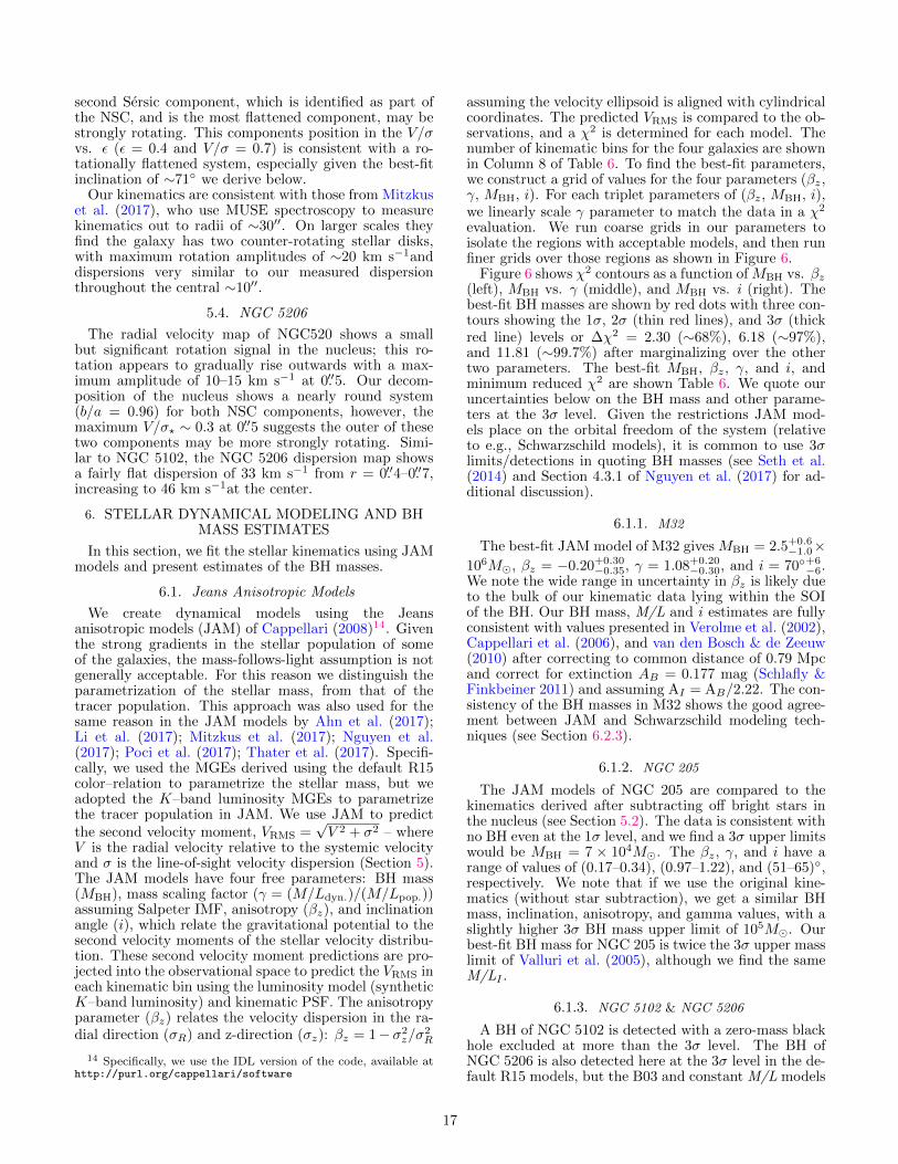
second Sersic component, which is identified as part ofthe NSC, and is the most flattened component, may bestrongly rotating. This components position in the V/σvs. ε (ε = 0.4 and V/σ = 0.7) is consistent with a ro-tationally flattened system, especially given the best-fitinclination of ∼71◦ we derive below.

Our kinematics are consistent with those from Mitzkuset al. (2017), who use MUSE spectroscopy to measurekinematics out to radii of ∼30′′. On larger scales theyfind the galaxy has two counter-rotating stellar disks,with maximum rotation amplitudes of ∼20 km s−1anddispersions very similar to our measured dispersionthroughout the central ∼10′′.

5.4. NGC 5206

The radial velocity map of NGC520 shows a smallbut significant rotation signal in the nucleus; this ro-tation appears to gradually rise outwards with a max-imum amplitude of 10–15 km s−1 at 0.′′5. Our decom-position of the nucleus shows a nearly round system(b/a = 0.96) for both NSC components, however, themaximum V/σ? ∼ 0.3 at 0.′′5 suggests the outer of thesetwo components may be more strongly rotating. Simi-lar to NGC 5102, the NGC 5206 dispersion map showsa fairly flat dispersion of 33 km s−1 from r = 0.′′4–0.′′7,increasing to 46 km s−1at the center.

6. STELLAR DYNAMICAL MODELING AND BHMASS ESTIMATES

In this section, we fit the stellar kinematics using JAMmodels and present estimates of the BH masses.

6.1. Jeans Anisotropic Models

We create dynamical models using the Jeansanisotropic models (JAM) of Cappellari (2008)14. Giventhe strong gradients in the stellar population of someof the galaxies, the mass-follows-light assumption is notgenerally acceptable. For this reason we distinguish theparametrization of the stellar mass, from that of thetracer population. This approach was also used for thesame reason in the JAM models by Ahn et al. (2017);Li et al. (2017); Mitzkus et al. (2017); Nguyen et al.(2017); Poci et al. (2017); Thater et al. (2017). Specifi-cally, we used the MGEs derived using the default R15color–relation to parametrize the stellar mass, but weadopted the K–band luminosity MGEs to parametrizethe tracer population in JAM. We use JAM to predictthe second velocity moment, VRMS =

√V 2 + σ2 – where

V is the radial velocity relative to the systemic velocityand σ is the line-of-sight velocity dispersion (Section 5).The JAM models have four free parameters: BH mass(MBH), mass scaling factor (γ = (M/Ldyn.)/(M/Lpop.))assuming Salpeter IMF, anisotropy (βz), and inclinationangle (i), which relate the gravitational potential to thesecond velocity moments of the stellar velocity distribu-tion. These second velocity moment predictions are pro-jected into the observational space to predict the VRMS ineach kinematic bin using the luminosity model (syntheticK–band luminosity) and kinematic PSF. The anisotropyparameter (βz) relates the velocity dispersion in the ra-dial direction (σR) and z-direction (σz): βz = 1− σ2

z/σ2R

14 Specifically, we use the IDL version of the code, available athttp://purl.org/cappellari/software

assuming the velocity ellipsoid is aligned with cylindricalcoordinates. The predicted VRMS is compared to the ob-servations, and a χ2 is determined for each model. Thenumber of kinematic bins for the four galaxies are shownin Column 8 of Table 6. To find the best-fit parameters,we construct a grid of values for the four parameters (βz,γ, MBH, i). For each triplet parameters of (βz, MBH, i),we linearly scale γ parameter to match the data in a χ2

evaluation. We run coarse grids in our parameters toisolate the regions with acceptable models, and then runfiner grids over those regions as shown in Figure 6.

Figure 6 shows χ2 contours as a function of MBH vs. βz(left), MBH vs. γ (middle), and MBH vs. i (right). Thebest-fit BH masses are shown by red dots with three con-tours showing the 1σ, 2σ (thin red lines), and 3σ (thickred line) levels or ∆χ2 = 2.30 (∼68%), 6.18 (∼97%),and 11.81 (∼99.7%) after marginalizing over the othertwo parameters. The best-fit MBH, βz, γ, and i, andminimum reduced χ2 are shown Table 6. We quote ouruncertainties below on the BH mass and other parame-ters at the 3σ level. Given the restrictions JAM mod-els place on the orbital freedom of the system (relativeto e.g., Schwarzschild models), it is common to use 3σlimits/detections in quoting BH masses (see Seth et al.(2014) and Section 4.3.1 of Nguyen et al. (2017) for ad-ditional discussion).

6.1.1. M32

The best-fit JAM model of M32 gives MBH = 2.5+0.6−1.0×

106M�, βz = −0.20+0.30−0.35, γ = 1.08+0.20

−0.30, and i = 70◦+6−6.

We note the wide range in uncertainty in βz is likely dueto the bulk of our kinematic data lying within the SOIof the BH. Our BH mass, M/L and i estimates are fullyconsistent with values presented in Verolme et al. (2002),Cappellari et al. (2006), and van den Bosch & de Zeeuw(2010) after correcting to common distance of 0.79 Mpcand correct for extinction AB = 0.177 mag (Schlafly &Finkbeiner 2011) and assuming AI = AB/2.22. The con-sistency of the BH masses in M32 shows the good agree-ment between JAM and Schwarzschild modeling tech-niques (see Section 6.2.3).

6.1.2. NGC 205

The JAM models of NGC 205 are compared to thekinematics derived after subtracting off bright stars inthe nucleus (see Section 5.2). The data is consistent withno BH even at the 1σ level, and we find a 3σ upper limitswould be MBH = 7 × 104M�. The βz, γ, and i have arange of values of (0.17–0.34), (0.97–1.22), and (51–65)◦,respectively. We note that if we use the original kine-matics (without star subtraction), we get a similar BHmass, inclination, anisotropy, and gamma values, with aslightly higher 3σ BH mass upper limit of 105M�. Ourbest-fit BH mass for NGC 205 is twice the 3σ upper masslimit of Valluri et al. (2005), although we find the sameM/LI .

6.1.3. NGC 5102 & NGC 5206

A BH of NGC 5102 is detected with a zero-mass blackhole excluded at more than the 3σ level. The BH ofNGC 5206 is also detected here at the 3σ level in the de-fault R15 models, but the B03 and constant M/L models

17

TABLE 6Gemini/NIFS and VLT/SINFONI Jeans modeling best-fit results

Object Filter Color–M/L MBH βz γ i No. of Bins χ2r χ2

r, noBH rg, dyn. rg, dyn.

(M�) (◦) (′′) (pc)(1) (2) (3) (4) (5) (6) (7) (8) (9) (10) (11) (12)

M32 F814WG R15 2.5+0.6−1.0 × 106 −0.20+0.30

−0.35 1.08+0.20−0.30 70.0+6.0

−6.0 1354 1.12 6.72 0.404 1.61

NGC 205 F814WG R15 2.5+4.7−2.5 × 104 0.27+0.07

−0.10 1.10+0.10−0.18 59.0+5.0

−8.0 256 1.24 1.20 0.033 0.14

NGC 5102 F547MG R15 8.8+4.2−6.6 × 105 0.15+0.16

−0.16 1.15+0.06−0.03 71.5+9.0

−4.0 1017 1.12 3.57 0.070 1.20

NGC 5206 F814WG R15 4.7+2.3−3.4 × 105 0.25+0.08

−0.12 1.06+0.05−0.05 44.0+8.5

−5.0 240 1.20 2.69 0.058 1.00

Note. — Column 1: galaxy name. Column 2: the filter in which the luminosity and mass models are constructed;the superscript D or G means the stellar mass profile that are constructed from the HST imaging or its GALFITmodel (see Table B6 for full listing of modeling results). Column 3: the color–M/L relation used to construct massmodels. Columns 4–7: the best-fit parameters and their 3σ error intervals of JAM models including dynamical BHmasses (MBH), anisotropies (βz), mass scaling factors (γ), and the inclination angles (i), respectively. Column 8:number of stellar kinematic measurement bins. Columns 9 and 10: the reduced χ2

r and χ2r, no BH of the best-fit JAM

models and no BH cases, respectively. Columns 11 and 12: the best-fit BH sphere-of-influence (SOI) in arcsec andparsecs.

are consistent with zero mass at the &4σ level. We em-phasize here this is the first time these BHs are clearly de-tected and these masses are measured in the sub-millionsolar mass regime with the properties listed in Table 6.

To illustrate the best-fit JAM models with and withouta BH, we plot 1D and 2D VRMS predicted by JAM andcompare them with their corresponding data in Figure 7and Figure 8, respectively. The 1D VRMS profiles showthe bi-weighted average over circular annuli as shown inthe top-right plots in Figure 5. Overplotted on this dataare the best fit models, those with the maximum andminimum BH mass in the 3σ contours, and the best-fit noBH model. These show that models withMBH = 0M� donot provide a good fit to the data except for NGC 205.We quote both the corresponding χ2

r and χ2r, no BH for the

best-fit with and without BH in Table 6.The 1D profiles show that the radial data agree quite

well with the models, with the only siginficant discrep-ancy being at the center of NGC 205. This may be due tomass model issues in NGC 205 due both to the partiallyresolved kinematic data and the strong color gradientnear the center. However, we also note the dispersionmeasurements are very low, falling below the instrumen-tal resolution of the telescope (σLSF ∼ 23 km s−1).

With the best-fit BH mass value, the SOI is calculatedbased on the dynamics: rg, dyn. = GMBH/σ

2, where σ?is the stellar velocity dispersion of the bulge, G is thegravitational constant. The calculations of σ will be dis-cussed in Section 8.2. Alternatively, we also estimatethese BH SOI via our mass profile with rg, ? is the radiusat which the enclosed stellar mass is equal to MBH (Mer-ritt 2013). The results of rg, dyn. of these BH SOI arepresented in Table 6 in both arc-second (Column 10)and pc (Column 11) scales. Both methods give consis-tent values of BH SOI (rg, dyn. ' rg, ?). The rg, dyn. of∼0.′′07 and ∼0.′′06 in NGC 5102 and NGC 5206 are com-parable to the FWHMs of the data, suggesting that theobservational signature of these BHs are just marginallyresolved, while in M32, its BH’s signature is easily re-solved by our PSF. For NGC 205, its 3σ upper limit SOI(.0.′′03) is comparable to the resolution of ACS HRCimaging.

6.2. Sources of BH Mass Uncertainty

In this section, we discuss possible sources of uncertain-ties in our dynamical models for BH mass measurements.The confidence intervals in our analysis are based on thekinematic measurement errors but do not include anysystematic uncertainties in mass models, uncertaintiesin the PSF (particularly for NGC 5206), and uncertain-ties due to the JAM dynamical model that we used. Wefocus on these uncertainties here, and show that for ourMBH estimates, these systematics are smaller than thequoted 3σ confidence intervals.

6.2.1. Uncertainties due to Mass Models

We examine the mass model uncertainties by analyzingJAM model results from using (1) models with constantM/L or constructed using the B03 color–M/L correlation,(2) models based on different HST filters, and (3) modelsfit directly to the HST imaging rather than based on theGALFIT model results. Our tests show that our BHmass results do not strongly depend on the mass modelswe use for M32, NGC 205, and NGC 5102, although insome cases the best-fit γ vary significantly because thecenters of the galaxies are bluer than their surroundings.For NGC 5206, the constant M/L or B03 models arebasically consistent at the 3σ level with no BH, althoughthe best-fit BH from this model is still within our 3σuncertainties. We note that the color gradient in thecentral 1” is quite modest, but the R15 model predicts10% lower mass at the center than the other two massmodels. The complete results of these mass model testare given in detail in Table B6.

(a) Existing Color–M/L Models: We use the R15color–M/L relation for our default mass models (Sec-tion 6.1). Here we examine how much our JAM modelingresults would change if we use the shallower B03 color–M/L relation, or a constant M/L to construct our massmodels. Because our target galaxies are mostly bluer attheir centers (except for M32), we expect that the use ofa constant M/L will reduce the significance of any BHcomponent due to the increased stellar mass at the cen-ter relative to our reference R15 model. We show thebest-fit JAM model parameters using these alternative

18

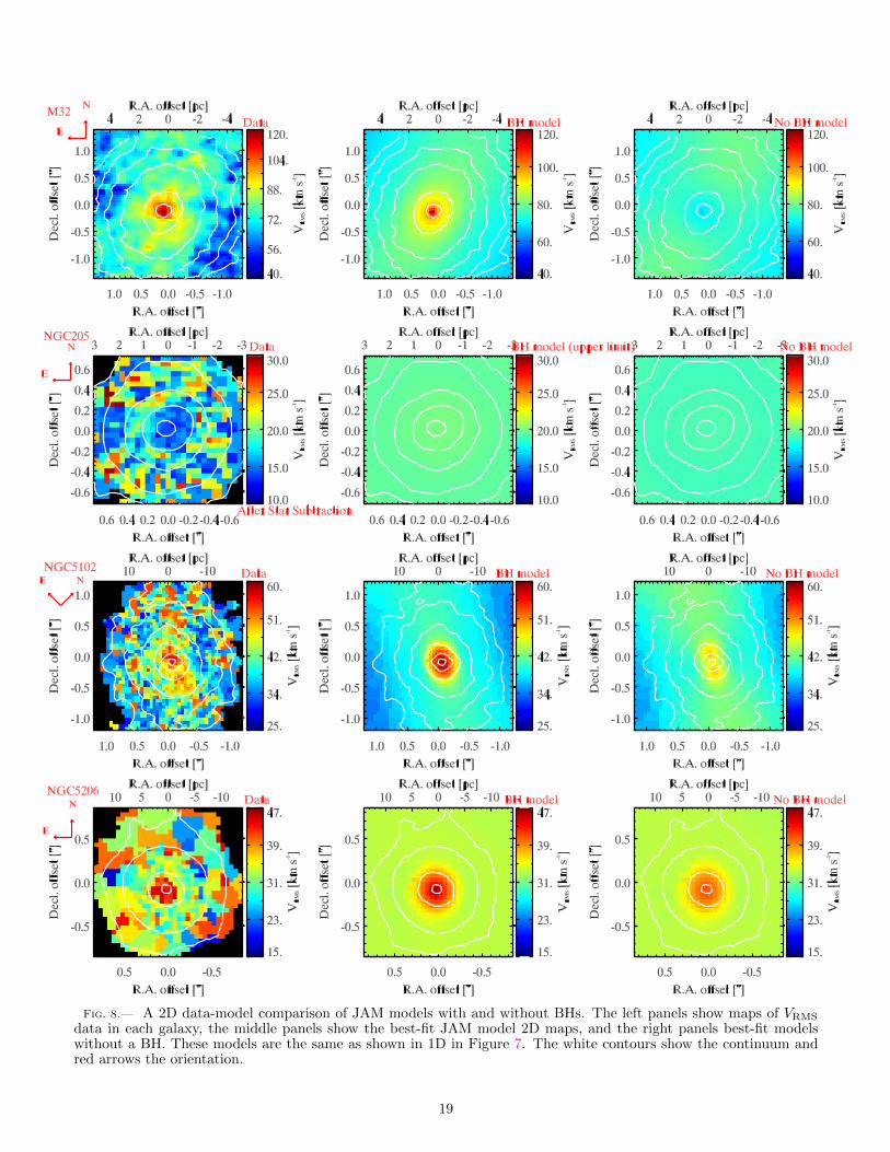
Fig. 8.— A 2D data-model comparison of JAM models with and without BHs. The left panels show maps of VRMS

data in each galaxy, the middle panels show the best-fit JAM model 2D maps, and the right panels best-fit modelswithout a BH. These models are the same as shown in 1D in Figure 7. The white contours show the continuum andred arrows the orientation.

19

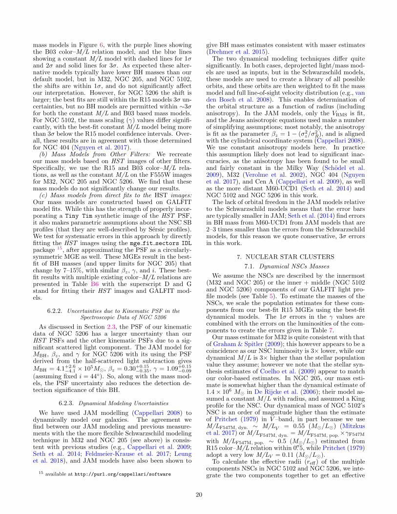
mass models in Figure 6, with the purple lines showingthe B03 color–M/L relation model, and the blue linesshowing a constant M/L model with dashed lines for 1σand 2σ and solid lines for 3σ. As expected these alter-native models typically have lower BH masses than ourdefault model, but in M32, NGC 205, and NGC 5102,the shifts are within 1σ, and do not significantly affectour interpretation. However, for NGC 5206 the shift islarger; the best fits are still within the R15 models 3σ un-certainties, but no BH models are permitted within ∼3σfor both the constant M/L and B03 based mass models.For NGC 5102, the mass scaling (γ) values differ signifi-cantly, with the best-fit constant M/L model being morethan 3σ below the R15 model confidence intervals. Over-all, these results are in agreement with those determinedfor NGC 404 (Nguyen et al. 2017).

(b) Mass Models from Other Filters: We recreateour mass models based on HST images of other filters.Specifically, we use the R15 and B03 color–M/L rela-tions, as well as the constant M/L on the F555W imagesfor M32, NGC 205 and NGC 5206. We find that thesemass models do not significantly change our results.

(c) Mass models from direct fits to the HST images:Our mass models are constructed based on GALFITmodel fits. While this has the strength of properly incor-porating a Tiny Tim synthetic image of the HST PSF,it also makes parametric assumptions about the NSC SBprofiles (that they are well-described by Sersic profiles).We test for systematic errors in this approach by directlyfitting the HST images using the mge fit sectors IDLpackage 15, after approximating the PSF as a circularly-symmetric MGE as well. These MGEs result in the best-fit of BH masses (and upper limits for NGC 205) thatchange by 7–15%, with similar βz, γ, and i. These best-fit results with multiple existing color–M/L relations arepresented in Table B6 with the superscript D and Gstand for fitting their HST images and GALFIT mod-els.

6.2.2. Uncertainties due to Kinematic PSF in theSpectroscopic Data of NGC 5206

As discussed in Section 2.3, the PSF of our kinematicdata of NGC 5206 has a larger uncertainty than ourHST PSFs and the other kinematic PSFs due to a sig-nificant scattered light component. The JAM model forMBH, βz, and γ for NGC 5206 with its using the PSFderived from the half-scattered light subtraction givesMBH = 4.1+2.6

−4.1 × 105M�, βz = 0.30+0.15−0.35, γ = 1.09+0.15

−0.09

(assuming fixed i = 44◦). So, along with the mass mod-els, the PSF uncertainty also reduces the detection de-tection significance of this BH.

6.2.3. Dynamical Modeling Uncertainties

We have used JAM modelling (Cappellari 2008) todynamically model our galaxies. The agreement wefind between our JAM modeling and previous measure-ments with the the more flexible Schwarzschild modelingtechnique in M32 and NGC 205 (see above) is consis-tent with previous studies (e.g., Cappellari et al. 2009;Seth et al. 2014; Feldmeier-Krause et al. 2017; Leunget al. 2018), and JAM models have also been shown to


give BH mass estimates consistent with maser estimates(Drehmer et al. 2015).

The two dynamical modeling techniques differ quitesignificantly. In both cases, deprojected light/mass mod-els are used as inputs, but in the Schwarzschild models,these models are used to create a library of all possibleorbits, and these orbits are then weighted to fit the massmodel and full line-of-sight velocity distribution (e.g., vanden Bosch et al. 2008). This enables determination ofthe orbital structure as a function of radius (includinganisotropy). In the JAM models, only the VRMS is fit,and the Jeans anisotropic equations used make a numberof simplifying assumptions; most notably, the anisotropyis fit as the parameter βz = 1− (σ2

z/σ2R), and is aligned

with the cylindrical coordinate system (Cappellari 2008).We use constant anisotropy models here. In practicethis assumption likely does not lead to significant inac-curacies, as the anisotropy has been found to be smalland fairly constant in the Milky Way (Schodel et al.2009), M32 (Verolme et al. 2002), NGC 404 (Nguyenet al. 2017), and Cen A (Cappellari et al. 2009), as wellas the more distant M60-UCD1 (Seth et al. 2014) andNGC 5102 and NGC 5206 in this work.

The lack of orbital freedom in the JAM models relativeto the Schwarzschild models means that the error barsare typically smaller in JAM; Seth et al. (2014) find errorsin BH mass from M60-UCD1 from JAM models that are2–3 times smaller than the errors from the Schwarzschildmodels, for this reason we quote conservative, 3σ errorsin this work.

7. NUCLEAR STAR CLUSTERS

7.1. Dynamical NSCs Masses

We assume the NSCs are described by the innermost(M32 and NGC 205) or the inner + middle (NGC 5102and NGC 5206) components of our GALFIT light pro-file models (see Table 5). To estimate the masses of theNSCs, we scale the population estimates for these com-ponents from our best-fit R15 MGEs using the best-fitdynamical models. The 1σ errors in the γ values arecombined with the errors on the luminosities of the com-ponents to create the errors given in Table 7.

Our mass estimate for M32 is quite consistent with thatof Graham & Spitler (2009); this however appears to be acoincidence as our NSC luminosity is 3× lower, while ourdynamical M/L is 3× higher than the stellar populationvalue they assume; however we note that the stellar syn-thesis estimates of Coelho et al. (2009) appear to matchour color-based estimates. In NGC 205, our mass esti-mate is somewhat higher than the dynamical estimate of1.4× 106 M� in De Rijcke et al. (2006); their model as-sumed a constant M/L with radius, and assumed a Kingprofile for the NSC. Our dynamical mass of NGC 5102’sNSC is an order of magnitude higher than the estimateof Pritchet (1979) in V –band, in part because we useM/LF547M, dyn. ∼ M/LV = 0.55 (M�/L�) (Mitzkuset al. 2017) or M/LF547M, dyn. = M/LF547M, pop.×γF547M

with M/LF547M, pop. ∼ 0.5 (M�/L�) estimated fromR15 color–M/L relation within 0.′′5, while Pritchet (1979)adopt a very low M/LV = 0.11 (M�/L�).

To calculate the effective radii (reff) of the multiplecomponents NSCs in NGC 5102 and NGC 5206, we inte-grate the two components together to get an effective

20

TABLE 7Dynamical Nuclear Star Cluster Properties

Object Filter reff. reff. µNSC L? M?,dyn. M/Lpop.,NSC ρreff. trelaxation

(′′) (pc) (mag) (×107L�) (×107M�) (M�/L�) (M� pc−3) (yrs)(1) (2) (3) (4) (5) (6) (7) (8) (9) (10)

M32 F814W 1.1 ± 0.1 4.4 ± 0.4 11.0 ± 0.1 1.10 ± 0.10 1.65 ± 0.31 1.35 1.1 × 105 6.8 × 109

NGC 205 F814W 0.3 ± 0.1 1.3 ± 0.4 13.6 ± 0.4 0.10 ± 0.04 0.20 ± 0.10 1.80 2.4 × 104 5.8 × 108

NGC 5102 F547M 1.6 ± 0.1 26.3 ± 1.6 12.1 ± 0.2 12.51 ± 2.49 7.30 ± 2.34 0.50 2.0 × 103 3.8 × 1010

NGC 5206 F814W 0.5 ± 0.1 8.1 ± 1.7 14.4 ± 0.2 0.73 ± 0.16 1.54 ± 0.51 1.98 3.8 × 103 2.0 × 1010

Note. — Columns 1: host galaxy name. Column 2: the filter used for the lumiosity modeling. Columns 3 and 4:the effective radii of NSCs in arcseconds and parsecs. Column 5: the total apparent magnitude of each NSC. Notethat the total apparent magnitude of M32 and NGC 205’s NSCs are taken from Table 5, while those of NGC 5102 andNGC 5206’s NSCs are estimated from their two inner Sersic components in Table 5. Columns 6 and 7: the luminosity(in filter from Column 2) and dynamical masses of NSCs. Here we assume the mass-scaling factor γ are calculated fromthe JAM dynamical models using the R15 color–M/L mass models. Column 8: the color-based population M/L in theband given in Column 2 (see Table 5). Column 9: the mass densities at the effective radii of the NSCs. Column 10:the relaxation timescales of the nuclei evaluated at the effective radii of NSCs.

104 105 106 107 108 109 1010

NSC Mass [MO • ]

1

10

100

r eff

, N

SC [

pc]

Georgiev+16 (ETG)Georgiev+16 (LTG)

N5102

N205

M32

N404N5206

FCC277

N4395

Walcher+05 (LTG)Rossa+06 (LTG)

Fig. 9.— Mass vs. size for NSCs. Our dynamicalmass determinations plus that of NGC 404 Nguyen et al.(2017) are shown in red (dots + outer circles); these arethe only dynamically determined NSC masses in early-type galaxies (ETGs). These are compared to photomet-ric estimates from Georgiev et al. (2016) plotted both inblack circles with central dots for ETGs and in blackopen circles for late-type galaxies (LTGs). LTG NSCswith the dynamical M/L estimates from Walcher et al.(2005) (late-type spirals) and the spectroscopic M/L es-timates Rossa et al. (2006) (Sa-Sbc) are plotted in bluepluses and diamonds, respectively. We also add the dy-namical M/L estimate for LTG NSC of NGC 4395 (denBrok et al. 2015) in yellow open circle and ETG NSC ofFCC 277 (Lyubenova et al. 2013) in the same notationof this work NSCs.

radius of 0.′′5 (8 pc) for NGC 5206 and 1.′′6 (26 pc)for NGC 5102. In Figure 9, we compare the sizes anddynamical masses of our ETG NSCs to previous mea-

surements in other galaxies. Most of the previous mea-surements are photometric mass estimates taken fromGeorgiev et al. (2016). The dynamical M/L estimatesare taken from Walcher et al. (2005) for LTGs, Lyuben-ova et al. (2013) for FCC 277, den Brok et al. (2015) forNGC 4395, Nguyen et al. (2017) for NGC 404, and thespectroscopic M/L estimates are taken from Rossa et al.(2006) for LTGs; we note here that our data are the firstsample of dynamical NSC masses measured in ETGs. Wefind that all four of our NSCs fall within the existing dis-tribution in the size-mass plane, with M32 and NGC 205being on the compact side of the distribution.

7.2. Uncertainties on NSC Mass Estimates

For the quoted errors in the NSC masses shown in Ta-ble 7, we take the 3σ errors on the mass scaling factors,and combine these in quadrature with uncertainties inthe total luminosity of the NSCs to provide a conserva-tive error estimate. The uncertainty in the total lumi-nosity of the NSC (which comes from how much of thecenter is considered to be part of the NSC) ends up be-ing the dominant error. The total fractional errors rangebetween 11% and 21%. In addition to these errors, weconsider the systematic error on the mass estimates fromusing different color–M/L relations. We find that themaximum differences are <12%, given that these are be-low the quoted uncertainties in all cases, we don’t quoteseparate systematic errors.

7.3. Structural Complexity and NSC formation

The NSCs of NGC 5102 and NGC 5206 have complexmorphologies, made up of multiple components, whileNGC 205 also shows clear color gradients within the nu-cleus. A similarly complex structure has also been seen inthe NSC of nearby ETG NGC 404, where a central lightexcess in the central 0.′′2 (3 pc) appears to be counter-rotating relative to the rest of the NSC (Seth et al. 2010)and has an age of ∼1 Gyr (Nguyen et al. 2017). Thesizes of NSCs in spirals also change with wavelength,with bluer bands having smaller sizes and being moreflattened, suggesting young populations are concentratednear the center (Seth et al. 2006; Georgiev & Boker 2014;Carson et al. 2015). In NGC 5102, the central compo-nent dominates the light within the central 0.′′2 (3 pc),while in NGC 5206, the central component dominates

21

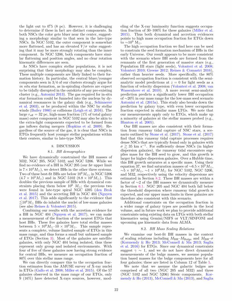
the light out to 0.′′5 (8 pc). However, it is challengingto determine if these in fact are distinct components. Inboth NSCs the color gets bluer near the center, suggest-ing a morphology similar to that seen in the late-typeNSCs. In NGC 5102, the outer component is somewhatmore flattened, and has an elevated V/σ value suggest-ing that it may be more strongly rotating than the innercomponent. In NGC 5206, both components have simi-lar flattening and position angles, and no clear rotationkinematic differences are seen.

As NSCs have complex stellar populations, it is notsurprising that their morphology may also be complex.These multiple components are likely linked to their for-mation history. In particular, the central bluer/youngercomponents seen in 3/4 of our clusters strongly argue forin situ star formation, as in-spiraling clusters are expectto be tidally disrupted in the outskirts of any pre-existingcluster (e.g., Antonini 2013). The gas required for in-situstar formation could be funneled into the nucleus by dy-namical resonances in the galaxy disk (e.g., Schinnereret al. 2003), or be produced within the NSC by stellarwinds (Bailey 1980) or collisions (Leigh et al. 2016). Thelarge reff = 32 pc, high-mass fraction (1% of total galaxymass) outer component in NGC 5102 may also be akin tothe extra-light components expected to be formed fromgas inflows during mergers (Hopkins et al. 2009). Re-gardless of the source of the gas, it is clear that NSCs inETGs frequently host younger stellar populations withintheir centers, similar to late-type NSCs.

8. DISCUSSION

8.1. BH demographics

We have dynamically constrained the BH masses ofM32, NGC 205, NGC 5102, and NGC 5206. While wefind no evidence of a BH in NGC 205 (our 3σ upper limitis 7×104M�), we detect BHs in the other three systems.Two of these best-fit BHs are below 106M�, in NGC 5206(4.7 × 105M�) and in NGC 5102 (8.8 × 105M�). Thisdoubles the previous sample of BHs with dynamical con-straints placing them below 106 M�; the previous twowere found in late-type spiral NGC 4395 (den Broket al. 2015) and the accreting BH in NGC 404 (Nguyenet al. 2017). This adds significantly to the evidence that.106M� BHs do inhabit the nuclei of low-mass galaxies(see also Reines & Volonteri 2015).

Combining our results with the accretion evidence fora BH in NGC 404 (Nguyen et al. 2017), we can makea measurement of the fraction of the nearest ETGs thathost BHs. These five galaxies have total stellar massesbetween 5 × 108M�–10 × 109M�. This sample repre-sents a complete, volume limited sample of ETGs in thismass range, and thus forms a small but unbiased sampleof ETGs (Section 3). Most of the galaxies are satellitegalaxies, with only NGC 404 being isolated, thus theserepresent only group and isolated environments. Withfour of five of these galaxies now having strong evidencefor central BHs, we measure an occupation fraction of80% over this stellar mass range.

We can directly compare this to the occupation frac-tion estimates from the AMUSE survey of X-ray nucleiin ETGs (Gallo et al. 2008; Miller et al. 2015). Of the 57galaxies observed in the mass range of our ETGs, only9 (16%) have detected X-rays sources, however, mod-

eling of the X-ray luminosity function suggests occupa-tion fraction of 30–100% for these galaxies (Miller et al.2015). Thus both dynamical and accretion evidencespoints to high mass occupation fraction for ETGs downto ∼109 M�.

The high occupation fraction we find here can be usedto constrain the seed formation mechanism of BHs in theearly Universe. Our result appears to be more consistentwith the scenario where BH seeds are formed from theremnants of the first generation of massive stars (e.g.,Population III stars (light seeds), Volonteri et al. 2008;Volonteri 2010; Greene 2012; Reines & Comastri 2016),rather than heavier seeds. More specifically, the 80%observed occupation fraction is consistent with the semi-analytic model predictions at z = 0 for light seeds as afunction of velocity dispersion (Volonteri et al. 2008; vanWassenhove et al. 2010). A more recent semi-analyticprediction predicts a significantly lower BH occupationof ∼20% in our mass range for the low-mass seed scenarioAntonini et al. (2015a). This study also breaks down theprediction by galaxy type, with even lower occupationfraction expected in similar mass LTGs. We note thatour measurements apply only to ETGs, which make upa minority of galaxies at the stellar masses probed (e.g.,Blanton et al. 2005).

Our BH masses are also consistent with their forma-tion from runaway tidal capture of NSC stars, a sce-nario outlined by Stone et al. (2017). Stone et al. (2017)find that this runaway tidal capture processes requiresdense NSCs that are typically found only in galaxies withσ & 35 km s−1. For sufficiently dense NSCs (in higherdispersion galaxies), the runaway tidal encounters sup-plies mass for the BH seed to grow, and this growth islarger for higher dispersion galaxies. Over a Hubble time,this BH growth saturates at a specific mass. Using theirequation 37, we find saturation masses of ∼6.5×105M�,∼5 × 105M�, ∼1 × 106M� for NGC 5102, NGC 5206,and M32, respectively using the velocity dispersions areestimated in Section 8.2. These BH masses are within afactor of ∼2 of the BH masses we dynamically measurein Section 6.1. NGC 205 and NGC 404 both fall belowthe threshold dispersion where runaway tidal growth isexpected, and our upper mass limits in these galaxies aretherefore also consistent with this scenario.

Additional constraints on the occupation fraction ina wider range of galaxy types are possible in the localvolume, and in future work we plan to provide additionalconstraints using existing data on LTGs with both stellarkinematics using Gemini/NIFS or VLT/SINFONI andupcoming gas kinematic data from ALMA.

8.2. BH Mass Scaling Relations

We examine our best-fit BH masses in the contextof scaling relations including MBH–MBulge and MBH–σ(Kormendy & Ho 2013; McConnell & Ma 2013; Sagliaet al. 2016) for ETGs. Since our dynamical constraintssuggest γ ∼ 1, and we do not have direct dynamicalmeasurements of the bulge masses, we assume popula-tion based masses for the bulge components here for allfour galaxies; these are listed in Column 12 of Table 5.

We note that we assume the galactic bulges arecomprised of all two (NGC 205 and M32) and three(NGC 5102 and NGC 5206) Sersic components. Kor-mendy & Ho (2013), McConnell & Ma (2013), and Saglia

22

107 108 109 1010 1011 1012

MBULGE [MO • ]

105

106

107

108

109

1010M

BH [

MO • ]

105

106

107

108

109

1010

105

106

107

108

109

1010

Scott+13Saglia+16

ETGs

LTGs

N404

N4395

M32

N205

N5102

N5206

100σ [km s-1]

105

106

107

108

109

1010

MBH [MO • ]

105

106

107

108

109

1010

105

106

107

108

109

1010

MB

H [

MO • ]

M32

N5102

N5206

N205

N404

N4395

Kormendy+13McConnell+13Saglia+16

Fig. 10.— Our four low-mass early-type galaxies in context of the MBH–MBulge (left) and MBH–σ (right) scalingrelations. The data of both early-type galaxies (ETGs, black dots with open circles) and late-type galaxies (blackopen circles) are taken from the compilation of Saglia et al. (2016). The dotted-, dashed-, long dashed-, and solid-linesindicate their linear best-fit in log scale of the relations from Scott et al. (2013); McConnell & Ma (2013); Kormendy& Ho (2013), and Saglia et al. (2016) for early-type galaxies (LTGs), respectively. The BH masses of M32, NGC 5102,and NGC 5206 and 3σ upper limit mass of NGC 205 with the downward arrow are plotted in red dots + open circlesas in the legend. We also add BHs with dynamical masses below 106M�, including the dwarf AGN late-type galaxyNGC 4395 (yellow open circle; den Brok et al. 2015) and early-type galaxy NGC 404 (Nguyen et al. 2017).

et al. (2016) report the bulge mass and luminosity of M32are ∼4.5 × 108M� and ∼4 × 108L� (MV = −16.64),while our estimates of mass and luminosity from F814Ware MBulge ∼ 8.2 × 108M� and LBulge ∼ 4.5 × 108L�;these are consistent with Graham & Spitler (2009); Ko-rmendy & Bender (2009) estimated in I–band. ForNGC 205, McConnachie (2012) reports a total luminos-ity of MV = −16.5 (3× 108L�) and Angus et al. (2016)simulation gives a mass of 4.0 × 108M�. We find aconsistent luminosity but higher mass for the bulge of6.5× 108M� from F814W HST data.

Figure 10 shows the best-fit BH mass of M32 is withinthe scatter of the MBH–MBulge relations of Kormendy& Ho (2013), McConnell & Ma (2013), and Saglia et al.(2016). However, the best-fit BHs masses of NGC 205,NGC 5102, and NGC 5206 clearly fall below these MBH–MBulge relations by 1-2 orders of magnitude. Combinedwith other recent work on BH mass measurements inlow-mass systems, e.g., NGC 404 (Nguyen et al. 2017),NGC 4395 (den Brok et al. 2015), RGG118 (Baldassareet al. 2015), Pox52 (Barth et al. 2004; Thornton et al.2008), an increasing number of galaxies appear to fallbelow the BH mass vs. bulge mass relationship extrapo-lated from massive ETGs to the low-mass regime. Thissuggests that the MBH–MBulge relationship may steepenas suggested by Scott et al. (2013) for low-mass systemswith bulge mass <2×1010M�. Alternatively, the scalingrelations may just break down at these masses, with sig-nificant scatter to lower masses as also seen in the mega-maser BH measurements in spiral galaxies (Lasker et al.2016a; Greene et al. 2016). We note that this increasedscatter may occur at bulge masses where the occupationfraction also drops below unity.

Next, we explore these BHs in the context of the MBH–σ scaling correlation. While typically the dispersion usedis that estimated within the effective radius, we do not

have this information for all of our galaxies. For M32 andNGC 205, the σe have been measured by Ho et al. (2009)who measure the dispersions of 72.1 ± 1.9 km s−1and23.3± 3.7 km s−1 in a 2′′× 4′′ aperture, respectively. Toestimate the central velocity dispersions of NGC 5102and NGC 5206, we co-add all the spectra in the FOVof 1.′′5 and fit the resulting single spectrum with pPXFfor velocity dispersions. This gives dispersions of 42.3±1.1 km s−1 for NGC 5102 and 35.4 ± 1.0 km s−1 forNGC 5206.

8.3. Possibility of Collections of Dark Remnants

Recent work has suggested that mass segregation ofstellar mass BHs can occur on timescales well below therelaxation time (Bianchini et al. 2017), significantly en-hancing the central M/L of globular clusters. An en-hancement of M/L is in fact seen in the globular clusterM15 (den Brok et al. 2014a). This leads to the possibilitythat a significant number of stellar mass BHs could col-lect at the center of NSCs, leading to a false detection ofa massive BH. We note that the current simulations areof much lower mass systems than the massive NSCs wediscuss here, and that significant uncertainties exist onhow many BHs would segregate and be retained duringthis process. Nonetheless, we can get a sense of the max-imum dark mass that can plausibly be accumulated bystellar remnants. For a Solar metallicity population witha standard Kroupa IMF, ∼4% of the mass of the clus-ter will turn into stellar mass BHs (Shanahan & Gieles2015). This represents a maximum mass fraction of theNSCs that could be concentrated at the center with theretention fraction of BHs likely being much lower thanthis. The fraction of the NSC mass found in the BHin M32, NGC 205, NGC 5102, and NGC 5206 are 13%,<3.5%, 1.1%, and 3.3% of their NSC masses, respec-tively. Therefore, based on the mass fractions, apart fromM32, a collection of dark remnants is a possibility.

23

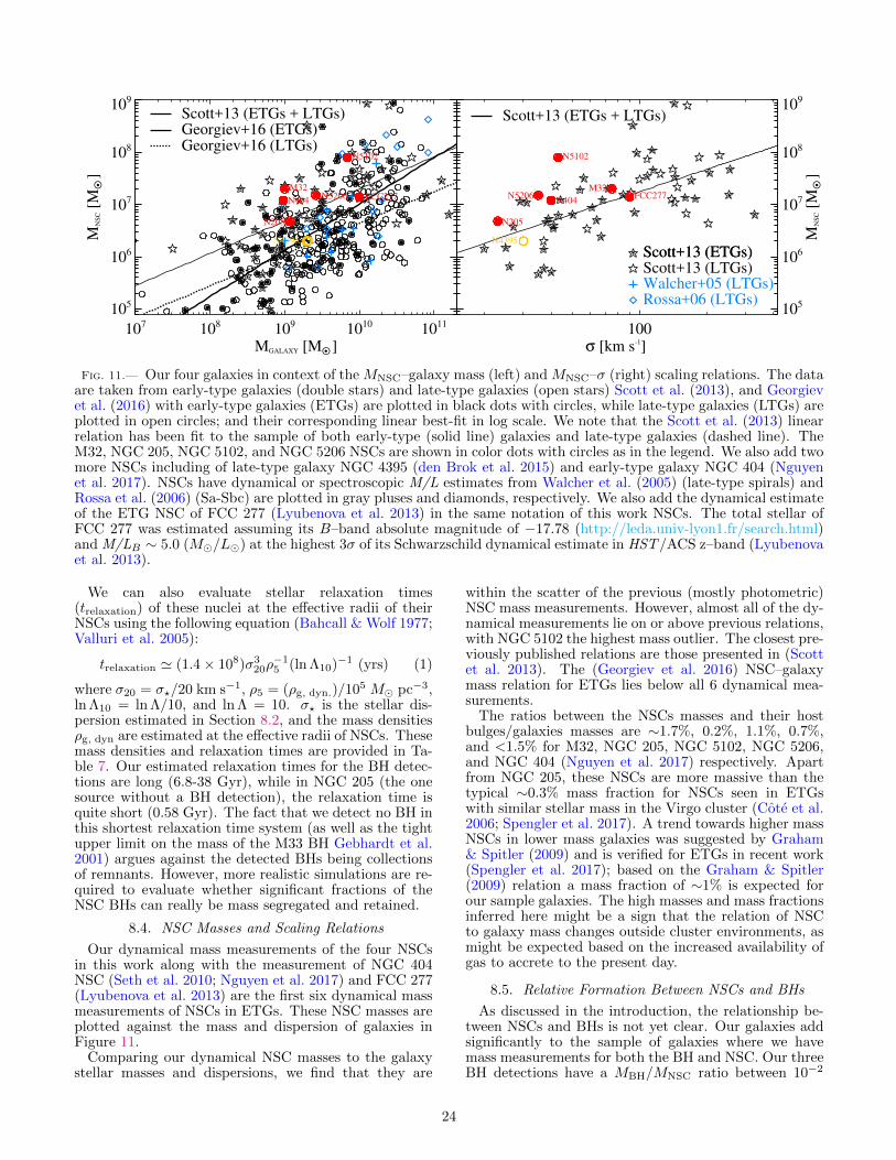
107 108 109 1010 1011

MGALAXY [MO • ]

105

106

107

108

109M

NS

C [

MO • ]

105

106

107

108

109

105

106

107

108

109

Scott+13 (ETGs + LTGs)Georgiev+16 (ETGs)Georgiev+16 (LTGs)

N404

N4395

M32

N205

N5102

N5206 FCC277

100σ [km s-1]

105

106

107

108

109

MBH [MO • ]

105

106

107

108

109

105

106

107

108

109

MN

SC [

MO • ]

N205

N5206 FCC277

N5102

N404

M32

Walcher+05 (LTGs)Rossa+06 (LTGs)

N4395

Scott+13 (ETGs)Scott+13 (LTGs)Scott+13 (ETGs)

Scott+13 (ETGs + LTGs)

Fig. 11.— Our four galaxies in context of the MNSC–galaxy mass (left) and MNSC–σ (right) scaling relations. The dataare taken from early-type galaxies (double stars) and late-type galaxies (open stars) Scott et al. (2013), and Georgievet al. (2016) with early-type galaxies (ETGs) are plotted in black dots with circles, while late-type galaxies (LTGs) areplotted in open circles; and their corresponding linear best-fit in log scale. We note that the Scott et al. (2013) linearrelation has been fit to the sample of both early-type (solid line) galaxies and late-type galaxies (dashed line). TheM32, NGC 205, NGC 5102, and NGC 5206 NSCs are shown in color dots with circles as in the legend. We also add twomore NSCs including of late-type galaxy NGC 4395 (den Brok et al. 2015) and early-type galaxy NGC 404 (Nguyenet al. 2017). NSCs have dynamical or spectroscopic M/L estimates from Walcher et al. (2005) (late-type spirals) andRossa et al. (2006) (Sa-Sbc) are plotted in gray pluses and diamonds, respectively. We also add the dynamical estimateof the ETG NSC of FCC 277 (Lyubenova et al. 2013) in the same notation of this work NSCs. The total stellar ofFCC 277 was estimated assuming its B–band absolute magnitude of −17.78 (http://leda.univ-lyon1.fr/search.html)and M/LB ∼ 5.0 (M�/L�) at the highest 3σ of its Schwarzschild dynamical estimate in HST/ACS z–band (Lyubenovaet al. 2013).

We can also evaluate stellar relaxation times(trelaxation) of these nuclei at the effective radii of theirNSCs using the following equation (Bahcall & Wolf 1977;Valluri et al. 2005):

trelaxation ' (1.4× 108)σ320ρ−15 (ln Λ10)−1 (yrs) (1)

where σ20 = σ?/20 km s−1, ρ5 = (ρg, dyn.)/105 M� pc−3,ln Λ10 = ln Λ/10, and ln Λ = 10. σ? is the stellar dis-persion estimated in Section 8.2, and the mass densitiesρg, dyn are estimated at the effective radii of NSCs. Thesemass densities and relaxation times are provided in Ta-ble 7. Our estimated relaxation times for the BH detec-tions are long (6.8-38 Gyr), while in NGC 205 (the onesource without a BH detection), the relaxation time isquite short (0.58 Gyr). The fact that we detect no BH inthis shortest relaxation time system (as well as the tightupper limit on the mass of the M33 BH Gebhardt et al.2001) argues against the detected BHs being collectionsof remnants. However, more realistic simulations are re-quired to evaluate whether significant fractions of theNSC BHs can really be mass segregated and retained.

8.4. NSC Masses and Scaling Relations

Our dynamical mass measurements of the four NSCsin this work along with the measurement of NGC 404NSC (Seth et al. 2010; Nguyen et al. 2017) and FCC 277(Lyubenova et al. 2013) are the first six dynamical massmeasurements of NSCs in ETGs. These NSC masses areplotted against the mass and dispersion of galaxies inFigure 11.

Comparing our dynamical NSC masses to the galaxystellar masses and dispersions, we find that they are

within the scatter of the previous (mostly photometric)NSC mass measurements. However, almost all of the dy-namical measurements lie on or above previous relations,with NGC 5102 the highest mass outlier. The closest pre-viously published relations are those presented in (Scottet al. 2013). The (Georgiev et al. 2016) NSC–galaxymass relation for ETGs lies below all 6 dynamical mea-surements.

The ratios between the NSCs masses and their hostbulges/galaxies masses are ∼1.7%, 0.2%, 1.1%, 0.7%,and <1.5% for M32, NGC 205, NGC 5102, NGC 5206,and NGC 404 (Nguyen et al. 2017) respectively. Apartfrom NGC 205, these NSCs are more massive than thetypical ∼0.3% mass fraction for NSCs seen in ETGswith similar stellar mass in the Virgo cluster (Cote et al.2006; Spengler et al. 2017). A trend towards higher massNSCs in lower mass galaxies was suggested by Graham& Spitler (2009) and is verified for ETGs in recent work(Spengler et al. 2017); based on the Graham & Spitler(2009) relation a mass fraction of ∼1% is expected forour sample galaxies. The high masses and mass fractionsinferred here might be a sign that the relation of NSCto galaxy mass changes outside cluster environments, asmight be expected based on the increased availability ofgas to accrete to the present day.

8.5. Relative Formation Between NSCs and BHs

As discussed in the introduction, the relationship be-tween NSCs and BHs is not yet clear. Our galaxies addsignificantly to the sample of galaxies where we havemass measurements for both the BH and NSC. Our threeBH detections have a MBH/MNSC ratio between 10−2

24

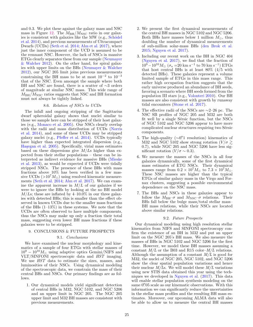
and 0.3. We plot these against the galaxy mass and NSCmass in Figure 12. The MBH/MNSC ratio in our galax-ies is consistent with galaxies like the MW (e.g., Schodelet al. 2014), and previous measurements of UltracompactDwarfs (UCDs) (Seth et al. 2014; Ahn et al. 2017), wherejust the inner component of the UCD is assumed to bethe remnant NSC. However, the lack of NSCs in massiveETGs clearly separates these from our sample (Neumayer& Walcher 2012). On the other hand, for spiral galax-ies with upper limits on the BHs (Neumayer & Walcher2012), our NGC 205 limit joins previous measurementsconstraining the BH mass to be at most 10−2 to 10−3

that of the NSC. Even amongst the sample where bothBH and NSC are found, there is a scatter of ∼3 ordersof magnitude at similar NSC mass. This wide range ofMBH/MNSC ratios suggests that NSC and BH formationmust not always be tightly linked.

8.6. Relation of NSCs to UCDs

The infall and ongoing stripping of the Sagittariusdwarf spheroidal galaxy shows that nuclei similar tothose we sample here can be stripped of their host galax-ies (e.g., Monaco et al. 2005). Our NSCs clearly overlapwith the radii and mass distribution of UCDs (Norriset al. 2014), and some of these UCDs may be strippedgalaxy nuclei (e.g., Pfeffer et al. 2014). UCDs typicallyhave higher than expected integrated dispersion (e.g.,Hasegan et al. 2005). Specifically, virial mass estimatesbased on these dispersions give M/Ls higher than ex-pected from their stellar populations – these can be in-terpreted as indirect evidence for massive BHs (Mieskeet al. 2013), as would be expected if UCDs were tidallystripped NSCs. The presence of these BHs with massfractions above 10% has been verified in a few mas-sive UCDs (>107M�) using resolved kinematic measure-ments (Seth et al. 2014; Ahn et al. 2017). We can exam-ine the apparent increase in M/L of our galaxies if wewere to ignore the BHs by looking at the no BH modelM/Ls; these are inflated by 4–10.0% in our three galax-ies with detected BHs; this is smaller than the effect ob-served in known UCDs due to the smaller mass fractionsof the BHs (1–13%) in these systems. We note that theUCDs are often observed to have multiple components,thus the NSCs may make up only a fraction their totalmass, suggesting even lower BH mass fractions if thesegalaxies were to be stripped.

9. CONCLUSIONS & FUTURE PROSPECTS

9.1. Conclusions

We have examined the nuclear morphology and kine-matics of a sample of four ETGs with stellar masses of109 − 1010M� using adaptive optics Gemini/NIFS andVLT/SINFONI spectroscopic data and HST imaging.We use HST data to estimate the sizes, masses, andluminosities of their NSCs. Using dynamical modelingof the spectroscopic data, we constrain the mass of theircentral BHs and NSCs. Our primary findings are as fol-lows.

1. Our dynamical models yield significant detectionof central BHs in M32, NGC 5102, and NGC 5206and an upper limit in NGC 205. The NGC 205upper limit and M32 BH masses are consistent withprevious measurements.

2. We present the first dynamical measurements ofthe central BH masses in NGC 5102 and NGC 5206.Both BHs have masses below 1 million M�, thusdoubling the number of dynamical measurementsof sub-million solar-mass BHs (den Brok et al.2015; Nguyen et al. 2017).

3. Including our recent work on the BH in NGC 404(Nguyen et al. 2017), we find that the fraction of109−1010M� (σ? =20 km s−1 to 70 km s−1) ETGsthat host central BHs is at least 80% (4/5 withdetected BHs). These galaxies represent a volumelimited sample of ETGs in this mass range. Thisrather high occupation fraction suggests that theearly universe produced an abundance of BH seeds,favoring a scenario where BH seeds formed from thepopulation III stars (e.g., Volonteri 2010). Our BHmasses are also consistent with growth by runawaytidal encounters (Stone et al. 2017).

4. The effective radii of the NSCs are ∼2–26 pc. TheNSC SB profiles of NGC 205 and M32 are bothfit well by a single Sersic function, but the NSCsof NGC 5102 and NGC 5206 appear to have morecomplicated nuclear structures requiring two Sersiccomponents.

5. The high-quality (∼0.′′1 resolution) kinematics ofM32 and NGC 5102 show strong rotation (V/σ &0.7), while NGC 205 and NGC 5206 have less sig-nificant rotation (V/σ ∼ 0.3).

6. We measure the masses of the NSCs in all fourgalaxies dynamically, some of the first dynamicalmass estimates of ETG NSCs. Their dynamicalmasses range from 0.2 × 107M� to 7.3 × 107M�.These NSC masses are higher than the typicalETGs of similar galaxy mass in the Virgo and For-nax clusters, suggesting a possible environmentaldependence on the NSC mass.

7. The BHs and NSCs in these galaxies appear tofollow the MBH–σ and MNSC–σ relations. TheirBHs fall below the bulge mass/total stellar mass–BH mass relations, while their NSCs are locatedabove similar relations.

9.2. Future Prospects

Our dynamical modeling using high resolution stellarkinematics from NIFS and SINFONI spectroscopy con-firm the existence of an BH in M32 and put an upperlimit on the NGC 205’s BH mass. We also measure themasses of BHs in NGC 5102 and NGC 5206 for the firsttime. However, we model these BH masses assuming aconstant M/L or the B03 and R15 color–M/L relations.Although the assumption of a constant M/L is good forM32, the nuclei of NGC 205, NGC 5102, and NGC 5206show the clear spatial population variations and hencetheir nuclear M/Ls. We will model these M/L variationsusing new STIS data obtained this year using the tech-niques we developed in Nguyen et al. (2017). This datawill enable stellar population synthesis modeling on thesame 0.′′05 scale as our kinematic observations. With thisinformation we can significantly reduce the uncertaintiesin the stellar mass profiles and the resulting BH mass es-timates. Moreover, our upcoming ALMA data will alsobe able to allow us to measure the central BH masses

25

107 108 109 1010 1011 1012

Galaxy Mass [MO • ]

10-4

10-2

100

102

104

MB

H/M

NS

C

10-4

10-2

100

102

104

10-4

10-2

100

102

104

Early-TypeLate-TypeEarly-Type

UCDs

N404N404N404N404N404

M32M32M32M32M32

N205N205N205N205N205

N5102N5102N5102N5102N5102

N5206N5206N5206N5206N5206

FCC277FCC277FCC277FCC277FCC277

M60-UCD1M60-UCD1M60-UCD1M60-UCD1M60-UCD1

VUCD3VUCD3VUCD3VUCD3VUCD3

M59cOM59cOM59cOM59cOM59cO

M31M31M31M31M31

MWMWMWMWMWN4395N4395N4395N4395N4395

106 107 108

MNSC [MO • ]

10-4

10-2

100

102

104

MB

H/M

NS

C

Early-TypeLate-Type

Early-Type

UCDs

N4395N4395N4395N4395N4395

M31M31M31M31M31

MWMWMWMWMW

M32M32M32M32M32

N5102N5102N5102N5102N5102

N5206N5206N5206N5206N5206

FCC277FCC277FCC277FCC277FCC277

N404N404N404N404N404N205N205N205N205N205

M60-UCD1M60-UCD1M60-UCD1M60-UCD1M60-UCD1VUCD3VUCD3VUCD3VUCD3VUCD3

M59cOM59cOM59cOM59cOM59cO

Fig. 12.— Ratio of the BH and NSC mass against their host-galaxy stellar mass (left) and their NSC dynamicalmasses based on dynamical measurements of M/Ldyn. (right). Original data with dynamical measurements are shownwith early- (black dots), late-type (gray dots) galaxies, and current BH mass measurements of UCDs (black stars)are taken from Neumayer & Walcher (2012), Graham & Spitler (2009), Lyubenova et al. (FCC 277; 2013), Seth et al.(M60-UCD1; 2014), and Ahn et al. (VUCD3 and M59cO; 2017). The upward/downward arrows are used for galaxieswith lower/upper limits of BH and NSC masses. We note that the for the UCD NSC masses, we plot only the massof their inner components.

using cold gas kinematic models of the circumnucleargas disk (CND) within the nuclei of a variety Hubbletype, nearby, and low-mass galaxy sample. This largerand high quality data sample will provide a more precise,complete, and unbiased occupation fraction dynamically.

The authors are grateful to Professor Elena Gallo ofThe University of Michigan, Department of Astronomyfor her refereeing role and provided comments thatsignificantly improved the presentation and accuracyof the paper. We also would like to thank AaronBarth of the Department of Physics and Astronomy,University of California, Irvine, Luis Ho and Li Zhao-Yuof the Department of Astronomy, School of Physics,Peking University for generously sharing us with theirNGC 5102 and NGC 5206 CGS SB profiles in fourBessel–Johnson filters BV RI; Iskren Y. Georgiev ofMax-Planck Instiut fur Astronomie for providing hisNSC data; and the Physics and Astronomy Department,University of Utah for supporting this work. D. D. N.and A. C. S. acknowledge financial support from NSFgrant AST-1350389. M. C. acknowledges support froma Royal Society University Research Fellowship.

Facilities: Gemini: Gemini/NIFS/ALTAIR, ESO–

VLT/SINFONI, and HST (WFPC2, ACS HRC)

APPENDIX

A. MEASUREMENT OF THE NGC 5102NUCLEUS (B − V )0 COLOR PROFILE

We determine (B−V )0 colors of NGC 5102 inside theradii of 0.′′4 from F450W–F569W WFPC2 data. How-ever, these data are saturated at the center. We can usethe F547M–F656N data to predict the central (B − V )0

colors where does not appear to be strong Hα emission.The upper panel of Figure A1 shows the scheme that weuse to explore the .0.′′4 (B − V )0 colors. First, we cre-ate the (F450W–F569W)0 and (F547M–F656N)0 colormaps with PSF cross convolution and Galactic extinc-tion correction in each band. Second, we get rid of allthe colors with saturated pixels from F450W and F569Win both (F450W–F569W)0 and (F547M–F656N)0 maps(balck dots). The pixels with possible contaminated byHα emission in F656N band were also eliminated basedon the criterion of (F547M–F656N)0 & 2.5×(F450W–F569W)0 (gray dots under the long-dashed line). All thegood pixels are presented in white-gray dots. Third, weuse these good pixels of colors to fit the linear correlationbetween (F450W–F569W)0 and (F547M–F656N)0. Thebest-fit is presented by the solid black line, while the scat-ter by 1σ of the fit is shown by the dashed black lines.The central (F450W–F569W)0 color profile is inferred

26

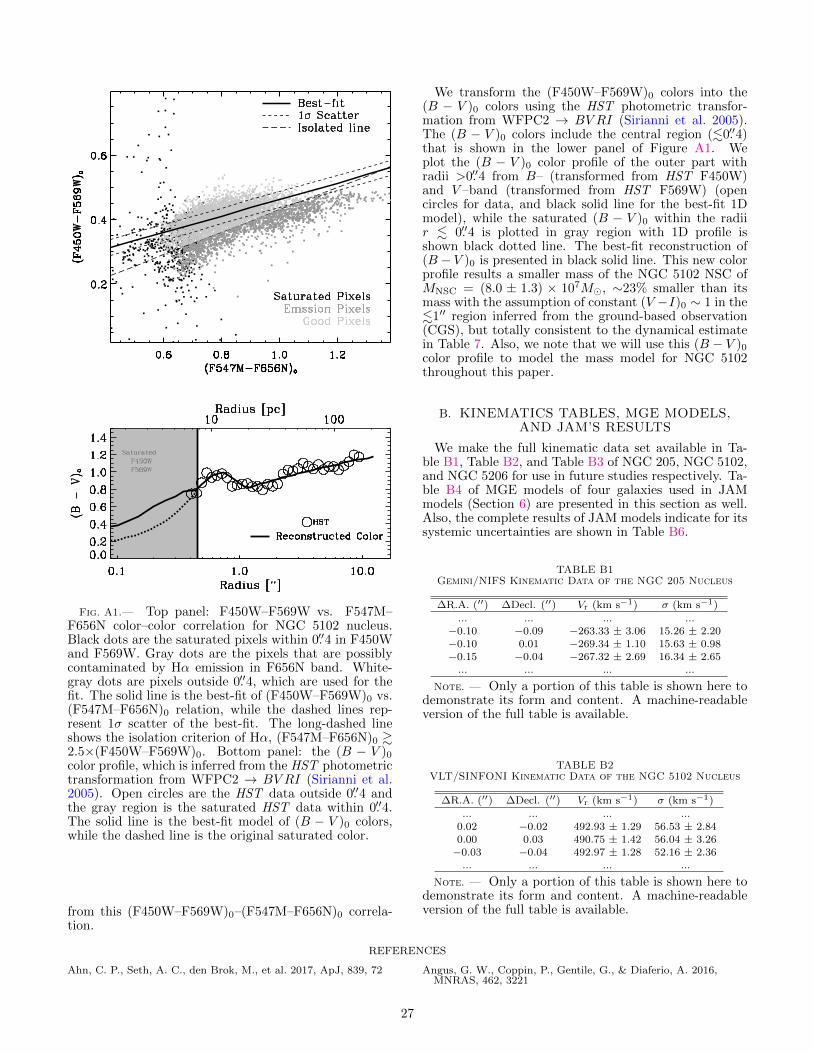
Fig. A1.— Top panel: F450W–F569W vs. F547M–F656N color–color correlation for NGC 5102 nucleus.Black dots are the saturated pixels within 0.′′4 in F450Wand F569W. Gray dots are the pixels that are possiblycontaminated by Hα emission in F656N band. White-gray dots are pixels outside 0.′′4, which are used for thefit. The solid line is the best-fit of (F450W–F569W)0 vs.(F547M–F656N)0 relation, while the dashed lines rep-resent 1σ scatter of the best-fit. The long-dashed lineshows the isolation criterion of Hα, (F547M–F656N)0 &2.5×(F450W–F569W)0. Bottom panel: the (B − V )0

color profile, which is inferred from the HST photometrictransformation from WFPC2 → BV RI (Sirianni et al.2005). Open circles are the HST data outside 0.′′4 andthe gray region is the saturated HST data within 0.′′4.The solid line is the best-fit model of (B − V )0 colors,while the dashed line is the original saturated color.

from this (F450W–F569W)0–(F547M–F656N)0 correla-tion.

We transform the (F450W–F569W)0 colors into the(B − V )0 colors using the HST photometric transfor-mation from WFPC2 → BV RI (Sirianni et al. 2005).The (B − V )0 colors include the central region (.0.′′4)that is shown in the lower panel of Figure A1. Weplot the (B − V )0 color profile of the outer part withradii >0.′′4 from B– (transformed from HST F450W)and V –band (transformed from HST F569W) (opencircles for data, and black solid line for the best-fit 1Dmodel), while the saturated (B − V )0 within the radiir . 0.′′4 is plotted in gray region with 1D profile isshown black dotted line. The best-fit reconstruction of(B − V )0 is presented in black solid line. This new colorprofile results a smaller mass of the NGC 5102 NSC ofMNSC = (8.0 ± 1.3) × 107M�, ∼23% smaller than itsmass with the assumption of constant (V −I)0 ∼ 1 in the.1′′ region inferred from the ground-based observation(CGS), but totally consistent to the dynamical estimatein Table 7. Also, we note that we will use this (B − V )0

color profile to model the mass model for NGC 5102throughout this paper.

B. KINEMATICS TABLES, MGE MODELS,AND JAM’S RESULTS

We make the full kinematic data set available in Ta-ble B1, Table B2, and Table B3 of NGC 205, NGC 5102,and NGC 5206 for use in future studies respectively. Ta-ble B4 of MGE models of four galaxies used in JAMmodels (Section 6) are presented in this section as well.Also, the complete results of JAM models indicate for itssystemic uncertainties are shown in Table B6.

TABLE B1Gemini/NIFS Kinematic Data of the NGC 205 Nucleus

∆R.A. (′′) ∆Decl. (′′) Vr (km s−1) σ (km s−1)

... ... ... ...−0.10 −0.09 −263.33 ± 3.06 15.26 ± 2.20−0.10 0.01 −269.34 ± 1.10 15.63 ± 0.98−0.15 −0.04 −267.32 ± 2.69 16.34 ± 2.65

... ... ... ...

Note. — Only a portion of this table is shown here todemonstrate its form and content. A machine-readableversion of the full table is available.

TABLE B2VLT/SINFONI Kinematic Data of the NGC 5102 Nucleus


... ... ... ...0.02 −0.02 492.93 ± 1.29 56.53 ± 2.840.00 0.03 490.75 ± 1.42 56.04 ± 3.26−0.03 −0.04 492.97 ± 1.28 52.16 ± 2.36

... ... ... ...


REFERENCES

Ahn, C. P., Seth, A. C., den Brok, M., et al. 2017, ApJ, 839, 72 Angus, G. W., Coppin, P., Gentile, G., & Diaferio, A. 2016,MNRAS, 462, 3221

27

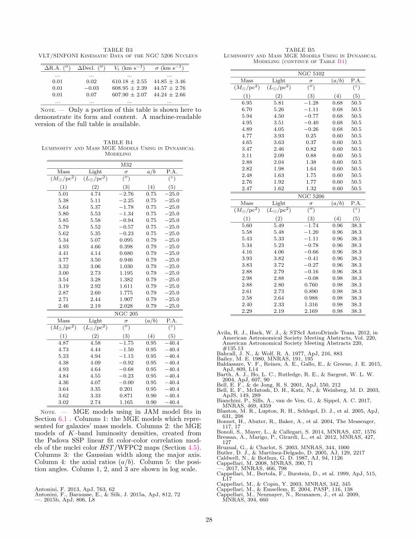
TABLE B3VLT/SINFONI Kinematic Data of the NGC 5206 Nucleus


... ... ... ...0.01 0.02 610.18 ± 2.55 44.85 ± 3.460.01 −0.03 608.95 ± 2.39 44.57 ± 2.760.01 0.07 607.90 ± 2.07 44.24 ± 2.66... ... ... ...


TABLE B4Luminosity and Mass MGE Models Using in Dynamical

Modeling

M32

Mass Light σ a/b P.A.

(M�/pc2) (L�/pc2) (′′) (◦)

(1) (2) (3) (4) (5)

5.01 4.74 −2.76 0.75 −25.05.38 5.11 −2.25 0.75 −25.05.64 5.37 −1.78 0.75 −25.05.80 5.53 −1.34 0.75 −25.05.85 5.58 −0.94 0.75 −25.05.79 5.52 −0.57 0.75 −25.05.62 5.35 −0.23 0.75 −25.05.34 5.07 0.095 0.79 −25.04.93 4.66 0.398 0.79 −25.04.41 4.14 0.680 0.79 −25.03.77 3.50 0.946 0.79 −25.03.32 3.06 1.030 0.79 −25.03.00 2.73 1.195 0.79 −25.03.54 3.28 1.382 0.79 −25.03.19 2.92 1.611 0.79 −25.02.87 2.60 1.775 0.79 −25.02.71 2.44 1.907 0.79 −25.02.46 2.19 2.028 0.79 −25.0

NGC 205

Mass Light σ (a/b) P.A.

(M�/pc2) (L�/pc2) (′′) (◦)

(1) (2) (3) (4) (5)

4.87 4.58 −1.75 0.95 −40.44.73 4.44 −1.50 0.95 −40.45.23 4.94 −1.15 0.95 −40.44.38 4.09 −0.92 0.95 −40.44.93 4.64 −0.68 0.95 −40.44.84 4.55 −0.23 0.95 −40.44.36 4.07 −0.00 0.95 −40.43.64 3.35 0.201 0.95 −40.43.62 3.33 0.871 0.90 −40.43.02 2.74 1.165 0.90 −40.4

Note. — MGE models using in JAM model fits inSection 6.1 . Columns 1: the MGE models which repre-sented for galaxies’ mass models. Columns 2: the MGEmodels of K–band luminosity densities, created fromthe Padova SSP linear fit color-color correlation mod-els of the nuclei color HST/WFPC2 maps (Section 4.5).Columns 3: the Gaussian width along the major axis.Column 4: the axial ratios (a/b). Column 5: the posi-tion angles. Colums 1, 2, and 3 are shown in log scale.

Antonini, F. 2013, ApJ, 763, 62Antonini, F., Barausse, E., & Silk, J. 2015a, ApJ, 812, 72—. 2015b, ApJ, 806, L8

TABLE B5Luminosity and Mass MGE Models Using in Dynamical

Modeling (continue of Table B4)

NGC 5102


(M�/pc2) (L�/pc2) (′′) (◦)

(1) (2) (3) (4) (5)

6.95 5.81 −1.28 0.68 50.56.70 5.26 −1.11 0.68 50.55.94 4.50 −0.77 0.68 50.54.95 3.51 −0.40 0.68 50.54.89 4.05 −0.26 0.68 50.54.77 3.93 0.25 0.60 50.54.65 3.63 0.37 0.60 50.53.47 2.46 0.82 0.60 50.53.11 2.09 0.88 0.60 50.52.88 2.04 1.38 0.60 50.52.82 1.98 1.64 0.60 50.52.48 1.63 1.75 0.60 50.52.76 1.92 1.77 0.60 50.52.47 1.62 1.32 0.60 50.5

NGC 5206


(M�/pc2) (L�/pc2) (′′) (◦)

(1) (2) (3) (4) (5)

5.60 5.49 −1.74 0.96 38.35.58 5.48 −1.20 0.96 38.35.43 5.33 −1.11 0.96 38.35.34 5.23 −0.78 0.96 38.34.16 4.06 −0.66 0.96 38.33.93 3.82 −0.41 0.96 38.33.83 3.72 −0.27 0.96 38.32.88 2.79 −0.16 0.96 38.32.98 2.88 −0.08 0.98 38.32.88 2.80 0.760 0.98 38.32.61 2.73 0.890 0.98 38.32.58 2.64 0.988 0.98 38.32.40 2.33 1.316 0.98 38.32.29 2.19 2.169 0.98 38.3

Avila, R. J., Hack, W. J., & STScI AstroDrizzle Team. 2012, inAmerican Astronomical Society Meeting Abstracts, Vol. 220,American Astronomical Society Meeting Abstracts 220,#135.13

Bahcall, J. N., & Wolf, R. A. 1977, ApJ, 216, 883Bailey, M. E. 1980, MNRAS, 191, 195Baldassare, V. F., Reines, A. E., Gallo, E., & Greene, J. E. 2015,

ApJ, 809, L14Barth, A. J., Ho, L. C., Rutledge, R. E., & Sargent, W. L. W.

2004, ApJ, 607, 90Bell, E. F., & de Jong, R. S. 2001, ApJ, 550, 212Bell, E. F., McIntosh, D. H., Katz, N., & Weinberg, M. D. 2003,

ApJS, 149, 289Bianchini, P., Sills, A., van de Ven, G., & Sippel, A. C. 2017,

MNRAS, 469, 4359Blanton, M. R., Lupton, R. H., Schlegel, D. J., et al. 2005, ApJ,

631, 208Bonnet, H., Abuter, R., Baker, A., et al. 2004, The Messenger,

117, 17Bonoli, S., Mayer, L., & Callegari, S. 2014, MNRAS, 437, 1576Bressan, A., Marigo, P., Girardi, L., et al. 2012, MNRAS, 427,

127Bruzual, G., & Charlot, S. 2003, MNRAS, 344, 1000Butler, D. J., & Martınez-Delgado, D. 2005, AJ, 129, 2217Caldwell, N., & Bothun, G. D. 1987, AJ, 94, 1126Cappellari, M. 2008, MNRAS, 390, 71—. 2017, MNRAS, 466, 798Cappellari, M., Bertola, F., Burstein, D., et al. 1999, ApJ, 515,

L17Cappellari, M., & Copin, Y. 2003, MNRAS, 342, 345Cappellari, M., & Emsellem, E. 2004, PASP, 116, 138Cappellari, M., Neumayer, N., Reunanen, J., et al. 2009,

MNRAS, 394, 660

28

TABLE B6Jeans modeling results (full table)

Object Filter Color–M/L MBH βz γ i Number of Bins χ2r rg rg

(M�) (◦) (′′) (pc)(1) (2) (3) (4) (5) (6) (7) (8) (9) (10) (11)

M32 F555WG R15 2.3+1.3−1.5 × 106 −0.25+0.35

−0.25 1.05+0.20−0.15 74+12

−9 1354 1.35 0.455 1.81

F555WD R15 2.5 × 106 −0.25 1.05 74 1.39 0.403 1.60

F814WG B03 2.0+0.5−0.8 × 106 −0.15+0.35

−0.35 1.07+0.14−0.10 72+6

−6 1.31 0.337 1.35

F814WG Conts 2.0+0.3−1.0 × 106 −0.20+0.40

−0.40 1.03+0.17−0.08 70+4

−5 1.97 0.337 1.35

F814WD R15 2.4 × 106 −0.20 1.08 70 1.75 0.387 1.61

F814WD B03 2.2 × 106 −0.15 1.05 72 1.83 0.319 1.35

F814WD Conts 2.1 × 106 −0.20 1.03 70 2.04 0.303 1.35

NGC 205 F555WD R15 2.7 × 104 0.27 1.07 60 256 1.33 0.070 0.30

F555WG∗ R15 2.1 × 104 0.25 1.07 60 1.37 0.051 0.17

F555WD∗ R15 3.0+3.2−3.0 × 104 0.27+0.08

−0.18 1.07+0.18−0.20 60+5

−8 197 1.37 0.074 0.35

F814WD∗ B03 2.0+4.0−2.0 × 104 0.25+0.06

−0.04 1.09+0.07−0.10 66+4

−8 1.40 0.063 0.22

F814WD∗ Const 1.8+3.2−1.8 × 104 0.27+0.04

−0.06 1.07+0.08−0.07 67+4

−7 2.51 0.060 0.20

NGC 5102 F547MG B03 7.0+10.0−2.0 × 105 0.25+0.08

−0.14 1.13+0.03−0.04 76.5+8.5

−6.0 1017 1.23 0.056 0.89

F547MG Const 6.0+9.0−3.5 × 105 0.09+0.08

−0.12 1.08+0.03−0.05 72.5+5.5

−4.5 2.32 0.048 0.76

F547MD R15 8.0 × 105 0.15 1.15 71.5 1.57 0.070 1.20

F547MD B03 7.5 × 105 0.18 1.13 76.0 1.73 0.056 0.89

F547MD Const 7.2 × 105 0.13 1.08 72.5 2.92 0.048 0.82

NGC 5206 F555WG R15 5.1+2.3−1.2 × 105 0.28+0.07

−0.14 1.08+0.20−0.40 43.5+4.0

−4.5 240 1.33 0.061 1.04

F555WD R15 4.8 × 105 0.28 1.08 43.5 1.36 0.071 1.21

F814WG B03 2.4+1.1−1.3 × 105 0.27+0.04

−0.15 1.10+0.05−0.10 41.0+2.5

−2.5 1.57 0.045 0.75

F814WG Const 2.1+0.8−1.4 × 105 0.29+0.06

−0.04 1.06+0.10−0.05 45.0+2.5

−1.5 2.41 0.038 0.65

F814WD R15 4.5 × 105 0.25 1.06 44.0 1.70 0.058 1.00

F814WD B03 2.3 × 105 0.27 1.10 41.0 1.66 0.045 0.75

F814WD Const 2.0 × 105 0.29 1.06 45.0 2.78 0.038 0.65

Note. — This table’s notations are the same in Table 6. Numbers without errors were fixed during JAM models fit-ting. For NGC 205, the filters with/without * means the best-fit models of after/before contaminated stars subtractionof the NIFS kinematic spectroscopy.

Cappellari, M., Bacon, R., Bureau, M., et al. 2006, MNRAS, 366,1126

Cardelli, J. A., Clayton, G. C., & Mathis, J. S. 1989, ApJ, 345,245

Carson, D. J., Barth, A. J., Seth, A. C., et al. 2015, AJ, 149, 170Coelho, P., Mendes de Oliveira, C., & Cid Fernandes, R. 2009,

MNRAS, 396, 624Corbin, M. R., O’Neil, E., & Rieke, M. J. 2001, AJ, 121, 2549Cote, P., Piatek, S., Ferrarese, L., et al. 2006, ApJS, 165, 57Davidge, T. J. 2003, ApJ, 597, 289—. 2005, AJ, 130, 2087—. 2008, AJ, 135, 1636—. 2015, ApJ, 799, 97De Rijcke, S., Prugniel, P., Simien, F., & Dejonghe, H. 2006,

MNRAS, 369, 1321Deharveng, J.-M., Jedrzejewski, R., Crane, P., Disney, M. J., &

Rocca-Volmerange, B. 1997, A&A, 326, 528den Brok, M., van de Ven, G., van den Bosch, R., & Watkins, L.

2014a, MNRAS, 438, 487den Brok, M., Peletier, R. F., Seth, A., et al. 2014b, MNRAS,

445, 2385den Brok, M., Seth, A. C., Barth, A. J., et al. 2015, ApJ, 809, 101Dong, X.-B., Ho, L. C., Yuan, W., et al. 2012, ApJ, 755, 167Drehmer, D. A., Storchi-Bergmann, T., Ferrari, F., Cappellari,

M., & Riffel, R. A. 2015, MNRAS, 450, 128Dressler, A., & Richstone, D. O. 1988, ApJ, 324, 701Eisenhauer, F., Abuter, R., Bickert, K., et al. 2003, in

Proc. SPIE, Vol. 4841, Instrument Design and Performance forOptical/Infrared Ground-based Telescopes, ed. M. Iye &A. F. M. Moorwood, 1548–1561

Emsellem, E., Monnet, G., & Bacon, R. 1994a, A&A, 285, 723

Emsellem, E., Monnet, G., Bacon, R., & Nieto, J.-L. 1994b,A&A, 285, 739

Fabian, A. C. 2012, ARA&A, 50, 455Feldmeier-Krause, A., Kerzendorf, W., Neumayer, N., et al. 2017,

MNRAS, 464, 194Ferrarese, L., Cote, P., Dalla Bonta, E., et al. 2006, ApJ, 644, L21Gallo, E., Treu, T., Jacob, J., et al. 2008, ApJ, 680, 154Gebhardt, K., Lauer, T. R., Kormendy, J., et al. 2001, AJ, 122,

2469Geha, M., Guhathakurta, P., Rich, R. M., & Cooper, M. C. 2006,

AJ, 131, 332Georgiev, I. Y., & Boker, T. 2014, MNRAS, 441, 3570Georgiev, I. Y., Boker, T., Leigh, N., Lutzgendorf, N., &

Neumayer, N. 2016, MNRAS, 457, 2122Graham, A. W. 2002, ApJ, 568, L13Graham, A. W., & Scott, N. 2015, ApJ, 798, 54Graham, A. W., & Spitler, L. R. 2009, MNRAS, 397, 2148Greene, J. E. 2012, Nature Communications, 3, 1304Greene, J. E., & Ho, L. C. 2007, ApJ, 670, 92Greene, J. E., Seth, A., Kim, M., et al. 2016, ApJ, 826, L32Guillard, N., Emsellem, E., & Renaud, F. 2016, MNRAS, 461,

3620Hasegan, M., Jordan, A., Cote, P., et al. 2005, ApJ, 627, 203Haring, N., & Rix, H.-W. 2004, ApJ, 604, L89Ho, L. C., Greene, J. E., Filippenko, A. V., & Sargent, W. L. W.

2009, ApJS, 183, 1Ho, L. C., Li, Z.-Y., Barth, A. J., Seigar, M. S., & Peng, C. Y.

2011, ApJS, 197, 21Ho, L. C., Terashima, Y., & Ulvestad, J. S. 2003, ApJ, 589, 783Hopkins, P. F., Lauer, T. R., Cox, T. J., Hernquist, L., &

Kormendy, J. 2009, ApJS, 181, 486

29

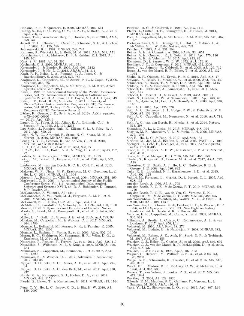
Hopkins, P. F., & Quataert, E. 2010, MNRAS, 405, L41Huang, S., Ho, L. C., Peng, C. Y., Li, Z.-Y., & Barth, A. J. 2013,

ApJ, 766, 47Husser, T.-O., Wende-von Berg, S., Dreizler, S., et al. 2013, A&A,

553, A6Jarrett, T. H., Chester, T., Cutri, R., Schneider, S. E., & Huchra,

J. P. 2003, AJ, 125, 525Jedrzejewski, R. I. 1987, MNRAS, 226, 747Kamann, S., Wisotzki, L., & Roth, M. M. 2013, A&A, 549, A71Karachentsev, I. D., Makarov, D. I., & Kaisina, E. I. 2013, AJ,

145, 101Kent, S. M. 1987, AJ, 94, 306Kochanek, C. S. 2016, MNRAS, 461, 371Kormendy, J., & Bender, R. 2009, ApJ, 691, L142Kormendy, J., & Ho, L. C. 2013, ARA&A, 51, 511Kraft, R. P., Nolan, L. A., Ponman, T. J., Jones, C., &

Raychaudhury, S. 2005, ApJ, 625, 785Krajnovic, D., Cappellari, M., de Zeeuw, P. T., & Copin, Y. 2006,

MNRAS, 366, 787Krajnovic, D., Cappellari, M., & McDermid, R. M. 2017, ArXiv

e-prints, arXiv:1707.04274Krist, J. 1995, in Astronomical Society of the Pacific Conference

Series, Vol. 77, Astronomical Data Analysis Software andSystems IV, ed. R. A. Shaw, H. E. Payne, & J. J. E. Hayes, 349

Krist, J. E., Hook, R. N., & Stoehr, F. 2011, in Society ofPhoto-Optical Instrumentation Engineers (SPIE) ConferenceSeries, Vol. 8127, Society of Photo-Optical InstrumentationEngineers (SPIE) Conference Series, 0

Lasker, R., Greene, J. E., Seth, A., et al. 2016a, ArXiv e-prints,arXiv:1602.06960

—. 2016b, ApJ, 825, 3Lauer, T. R., Faber, S. M., Ajhar, E. A., Grillmair, C. J., &

Scowen, P. A. 1998, AJ, 116, 2263Law-Smith, J., Ramirez-Ruiz, E., Ellison, S. L., & Foley, R. J.

2017, ApJ, 850, 22Leigh, N. W. C., Antonini, F., Stone, N. C., Shara, M. M., &

Merritt, D. 2016, MNRAS, 463, 1605Leung, G. Y. C., Leaman, R., van de Ven, G., et al. 2018,

MNRAS, arXiv:1803.02259Li, H., Ge, J., Mao, S., et al. 2017, ApJ, 838, 77Li, Z.-Y., Ho, L. C., Barth, A. J., & Peng, C. Y. 2011, ApJS, 197,

22Lodato, G., & Natarajan, P. 2006, MNRAS, 371, 1813Lotz, J. M., Telford, R., Ferguson, H. C., et al. 2001, ApJ, 552,

572Lyubenova, M., van den Bosch, R. C. E., Cote, P., et al. 2013,

MNRAS, 431, 3364Maksym, W. P., Ulmer, M. P., Eracleous, M. C., Guennou, L., &

Ho, L. C. 2013, MNRAS, 435, 1904Marconi, A., Risaliti, G., Gilli, R., et al. 2004, MNRAS, 351, 169Markwardt, C. B. 2009, in Astronomical Society of the Pacific

Conference Series, Vol. 411, Astronomical Data AnalysisSoftware and Systems XVIII, ed. D. A. Bohlender, D. Durand,& P. Dowler, 251

McConnachie, A. W. 2012, AJ, 144, 4McConnachie, A. W., Irwin, M. J., Ferguson, A. M. N., et al.

2005, MNRAS, 356, 979McConnell, N. J., & Ma, C.-P. 2013, ApJ, 764, 184McMillan, R., Ciardullo, R., & Jacoby, G. H. 1994, AJ, 108, 1610Merritt, D. 2013, Dynamics and Evolution of Galactic NucleiMieske, S., Frank, M. J., Baumgardt, H., et al. 2013, A&A, 558,

A14Miller, B. P., Gallo, E., Greene, J. E., et al. 2015, ApJ, 799, 98Mitzkus, M., Cappellari, M., & Walcher, C. J. 2017, MNRAS,

464, 4789Monaco, L., Bellazzini, M., Ferraro, F. R., & Pancino, E. 2005,

MNRAS, 356, 1396Monaco, L., Saviane, I., Perina, S., et al. 2009, A&A, 502, L9Moran, E. C., Shahinyan, K., Sugarman, H. R., Velez, D. O., &

Eracleous, M. 2014, AJ, 148, 136Natarajan, P., Pacucci, F., Ferrara, A., et al. 2017, ApJ, 838, 117Nayakshin, S., Wilkinson, M. I., & King, A. 2009, MNRAS, 398,

L54Neumayer, N., Cappellari, M., Reunanen, J., et al. 2007, ApJ,

671, 1329Neumayer, N., & Walcher, C. J. 2012, Advances in Astronomy,

2012, 709038Nguyen, D. D., Seth, A. C., Reines, A. E., et al. 2014, ApJ, 794,

34Nguyen, D. D., Seth, A. C., den Brok, M., et al. 2017, ApJ, 836,

237Norris, M. A., Kannappan, S. J., Forbes, D. A., et al. 2014,

MNRAS, 443, 1151Paudel, S., Lisker, T., & Kuntschner, H. 2011, MNRAS, 413, 1764

Peng, C. Y., Ho, L. C., Impey, C. D., & Rix, H.-W. 2010, AJ,139, 2097

Peterson, R. C., & Caldwell, N. 1993, AJ, 105, 1411Pfeffer, J., Griffen, B. F., Baumgardt, H., & Hilker, M. 2014,

MNRAS, 444, 3670Poci, A., Cappellari, M., & McDermid, R. M. 2017, MNRAS, 467,

1397Portegies Zwart, S. F., Baumgardt, H., Hut, P., Makino, J., &

McMillan, S. L. W. 2004, Nature, 428, 724Pritchet, C. 1979, ApJ, 231, 354Reines, A. E., & Comastri, A. 2016, PASA, 33, e054Reines, A. E., Greene, J. E., & Geha, M. 2013, ApJ, 775, 116Reines, A. E., & Volonteri, M. 2015, ApJ, 813, 82Richstone, D., & Sargent, W. L. W. 1972, ApJ, 176, 91Roediger, J. C., & Courteau, S. 2015, MNRAS, 452, 3209Rose, J. A., Arimoto, N., Caldwell, N., et al. 2005, AJ, 129, 712Rossa, J., van der Marel, R. P., Boker, T., et al. 2006, AJ, 132,

1074Saglia, R. P., Opitsch, M., Erwin, P., et al. 2016, ApJ, 818, 47Satyapal, S., Boker, T., Mcalpine, W., et al. 2009, ApJ, 704, 439Schinnerer, E., Boker, T., & Meier, D. S. 2003, ApJ, 591, L115Schlafly, E. F., & Finkbeiner, D. P. 2011, ApJ, 737, 103Schodel, R., Feldmeier, A., Kunneriath, D., et al. 2014, A&A,

566, A47Schodel, R., Merritt, D., & Eckart, A. 2009, A&A, 502, 91Scott, N., Graham, A. W., & Schombert, J. 2013, ApJ, 768, 76Seth, A., Agueros, M., Lee, D., & Basu-Zych, A. 2008, ApJ, 678,

116Seth, A. C. 2010, ApJ, 725, 670Seth, A. C., Dalcanton, J. J., Hodge, P. W., & Debattista, V. P.

2006, AJ, 132, 2539Seth, A. C., Cappellari, M., Neumayer, N., et al. 2010, ApJ, 714,

713Seth, A. C., van den Bosch, R., Mieske, S., et al. 2014, Nature,

513, 398Shanahan, R. L., & Gieles, M. 2015, MNRAS, 448, L94Sharina, M. E., Afanasiev, V. L., & Puzia, T. H. 2006, MNRAS,

372, 1259She, R., Ho, L. C., & Feng, H. 2017, ApJ, 842, 131Sirianni, M., Jee, M. J., Benıtez, N., et al. 2005, PASP, 117, 1049Spengler, C., Cote, P., Roediger, J., et al. 2017, ArXiv e-prints,

arXiv:1709.00406Stone, N. C., Kupper, A. H. W., & Ostriker, J. P. 2017, MNRAS,

467, 4180Stone, N. C., & Metzger, B. D. 2016, MNRAS, 455, 859Thater, S., Krajnovic, D., Bourne, M. A., et al. 2017, A&A, 597,

A18Thornton, C. E., Barth, A. J., Ho, L. C., Rutledge, R. E., &

Greene, J. E. 2008, ApJ, 686, 892Tully, R. B., Libeskind, N. I., Karachentsev, I. D., et al. 2015,

ApJ, 802, L25Valluri, M., Ferrarese, L., Merritt, D., & Joseph, C. L. 2005, ApJ,

628, 137van den Bergh, S. 1976, AJ, 81, 795van den Bosch, R. C. E., & de Zeeuw, P. T. 2010, MNRAS, 401,

1770van den Bosch, R. C. E., van de Ven, G., Verolme, E. K.,

Cappellari, M., & de Zeeuw, P. T. 2008, MNRAS, 385, 647van Wassenhove, S., Volonteri, M., Walker, M. G., & Gair, J. R.

2010, MNRAS, 408, 1139van Woerden, H., Schwarz, U. J., Peletier, R. F., & Wakker, B. P.

1996, in IAU Symposium, Vol. 171, New Light on GalaxyEvolution, ed. R. Bender & R. L. Davies, 464

Verolme, E. K., Cappellari, M., Copin, Y., et al. 2002, MNRAS,335, 517

Villaume, A., Brodie, J., Conroy, C., Romanowsky, A. J., & vanDokkum, P. 2017, ApJ, 850, L14

Volonteri, M. 2010, A&A Rev., 18, 279Volonteri, M., Lodato, G., & Natarajan, P. 2008, MNRAS, 383,

1079Volonteri, M., Reines, A. E., Atek, H., Stark, D. P., & Trebitsch,

M. 2017, ApJ, 849, 155Walcher, C. J., Boker, T., Charlot, S., et al. 2006, ApJ, 649, 692Walcher, C. J., van der Marel, R. P., McLaughlin, D., et al. 2005,

ApJ, 618, 237Wallace, L., & Hinkle, K. 1996, ApJS, 107, 312Wegner, G., Bernardi, M., Willmer, C. N. A., et al. 2003, AJ,

126, 2268Weigel, A. K., Schawinski, K., Treister, E., et al. 2015, MNRAS,

448, 3167Welch, D. L., Madore, B. F., McAlary, C. W., & McLaren, R. A.

1986, ApJ, 305, 583Wevers, T., van Velzen, S., Jonker, P. G., et al. 2017, MNRAS,

471, 1694Worthey, G. 2004, AJ, 128, 2826Xilouris, E. M., Madden, S. C., Galliano, F., Vigroux, L., &

Sauvage, M. 2004, A&A, 416, 41Yang, Y., Li, Z., Sjouwerman, L. O., et al. 2015, ApJ, 807, L19

30

Dieu D. Nguyen , Sebastian Kamann Michele Cappellari ... the number of low-mass galaxies with...

Documents

Transcript of Dieu D. Nguyen , Sebastian Kamann Michele Cappellari ... the number of low-mass galaxies with...