Diagnosing Drivers of Reservoir Sedimentation in the ...
63
Diagnosing Drivers of Reservoir Sedimentation in the Western US: A Case Study of Prineville Reservoir, Oregon By Leah C. Bensching B.S. Santa Clara University, 2016 A Thesis Submitted to the Faculty of the Graduate School of the University of Colorado in partial fulfillment Of the requirements for the degree of Master of Science Department of Civil, Environmental and Architectural Engineering 2018
Transcript of Diagnosing Drivers of Reservoir Sedimentation in the ...

Diagnosing Drivers of Reservoir Sedimentation in the Western US:
A Case Study of Prineville Reservoir, Oregon
By
Leah C. Bensching
B.S. Santa Clara University, 2016
A Thesis Submitted to the
Faculty of the Graduate School of the
University of Colorado in partial fulfillment
Of the requirements for the degree of
Master of Science
Department of Civil, Environmental and Architectural Engineering
2018
ii
This Thesis entitled: Diagnosing Drivers of Reservoir Sedimentation in the Western US:
A Case study on Prineville Reservoir
Written by Leah C. Bensching
has been approved for the Department of Civil, Environmental and Architectural Engineering
_________________________________
Prof. Ben Livneh
_________________________________
Prof. Joseph Kasprzyk
_________________________________
Dr. J. Toby Minear
_________________________________
Dr. Blair Greimann
Date: _________________
The final copy of this thesis has been examined by the signatories, and we find that both the
content and the form meet acceptable presentation standards of scholarly work in the above-
mentioned discipline.

iii
Bensching, Leah C. (M.S. Civil Engineering)
Diagnosing Drivers of Reservoir Sedimentation in the Western US:
A Case study of Prineville Reservoir
Thesis directed by Ben Livneh and Joseph Kasprzyk
Abstract
There is great need to quantify reservoir storage loss due to sediment. Less than 1% of
reservoirs in the US have more than one volume survey. Due to the lack of frequent data
collection, a constant rate sediment yield from year to year is often assumed. This study aims to
explore the following questions: 1) Can hydrologically-forced sediment algorithms help us
advance reservoir sedimentation estimates to improve future planning? 2) To which processes
and inputs are reservoir sedimentation estimates most sensitive? 3) What can we learn from
models that the linear sediment accumulation assumption fails to assess? It will address these
questions through a Sobol Sensitivity analysis a hydrologically forced sediment algorithm
ensemble, as well as an evaluation of differences between the hydrologically forced and linear
sedimentation assumptions. The hydrologic model used are Variable Infiltration Capacity (VIC)
which is coupled with sediment algorithms including the Modified Universal Soil Loss Equation
(MUSLE), Hydrological Simulation Program—Fortran (HSPF) and Systeme Hydrologique
European Sediment Model (SHE-SED) from within the Distributed Hydrology Soil Vegetation
Model (DHSVM). Sediment accumulation will be modeled for Prineville Reservoir near Bend,
Oregon.

iv
Dedication
To my Grandmother who was my biggest cheerleader and believed I could accomplish all of my
goals.
To my godfather, who was a constant reminder of the love and support sounding me.

v
Acknowledgements
I would like to acknowledge Dr. Blair Greimann and the US Bureau of Reclamation for
collaboration on this work, sharing his expertise, and identification of the case study location
chosen for study in this thesis.
I would also like to thank Ben Livneh for being my advisor and guide from my first day at CU.
Thank you for your wisdom through this process. Most of all, thank you for your constant
encouragement and understanding throughout some tough times.
Thank you, Joe Kasprzyk for joining this research effort and becoming a co-advisor. Your
knowledge and guidance greatly benefited the final product.
Most of all thank you to Laura Doyle, my undergraduate advisor, who brought out my love and
passion for water resources.
Lastly, I would like to thank my village without whom I would be completing my masters. The
CEAE TA’s who were my first friends in a new city. My roommates, Lauren, Karen and Heather
who helped our apartment feel like a home. Kathy and Brad Arehart for being my second family
and welcoming me into their home. My family for support throughout my entire education. The
community with in the BAM swim team who helped me find a place to destress. And finally, the
doctors who help me learn to cope with a challenging medical condition.

vi
Table of Contents
Chapter 1: Introduction & Background ....................................................................................... 1
1.1 Overview .......................................................................................................................................... 1
1.2 Introduction & Motivation ............................................................................................................ 2
1.3 Diagnosing Sedimentation ............................................................................................................. 3
1.4 Sediment Development and Transport ......................................................................................... 4
1.6 Sediment Modeling ......................................................................................................................... 6
1.7 Sediment Management Techniques .............................................................................................. 8
1.8 Summary of Chapters .................................................................................................................... 9
Chapter 2: Methods ...................................................................................................................... 11
Overview ....................................................................................................................................... 11
2.1 Study Area ..................................................................................................................................... 12
2.2 Data Sources ................................................................................................................................. 14
2.3 Hydrologic Model and Sediment Algorithms ............................................................................ 15
2.3.1 Hydrologic Model – Variable Infiltration Capacity model .................................................................. 15 2.3.2 Sediment Ensemble .............................................................................................................................. 16
Critical Area Approach ....................................................................................................................... 20
Modeling Assumptions for Reservoir Sedimentation ......................................................................... 20
2.4 Sobol Sensitivity Analysis ............................................................................................................ 21
2.4.1 Theory .................................................................................................................................................. 21 2.4.2 Application ........................................................................................................................................... 23
2.5 Model Performance Measures ..................................................................................................... 25
2.6 Sediment Yield Linearity ............................................................................................................. 28
Chapter 3: Results ........................................................................................................................ 30
3.1 Streamflow Sensitivity.................................................................................................................. 30
3.2 Streamflow Model Selection ........................................................................................................ 32
3.3 Reservoir Sediment Accumulation ............................................................................................. 34
3.4 Sediment Sensitivity Analysis ...................................................................................................... 37
3.5 Dotty Plots ..................................................................................................................................... 38
3.6 Linear Reservoir Sediment Accumulation Analysis .................................................................. 44
3.6.1 Root Mean Squared Difference ............................................................................................................ 44 3.6.2 Error Extrapolating Linear Projections ................................................................................................. 47
Chapter 4 Discussion & Conclusion ........................................................................................... 49
4.1 Streamflow Sensitivity.................................................................................................................. 49

vii
4.2 Streamflow Selection ................................................................................................................... 50`
4.3 The Linear Sediment Yield Assumption .................................................................................... 50
4.4 Future Work ................................................................................................................................. 51
4.5 Conclusion ..................................................................................................................................... 51
Works Cited .................................................................................................................................. 52
1
Chapter 1: Introduction & Background
1.1 Overview
There is great need to quantify reservoir storage loss due to sediment. Typically, the
difference between reservoir volume surveys is used to project future sediment loss. However,
less than 1% of reservoirs in the US have more than one reservoir volume survey. Due to the
lack of frequent data collection, a linearity assumption in the sediment yield is often made for the
time between surveys, meaning a constant rate sediment yield from year to year. This assumption
does not account for changing climate or the year-to-year variations in hydrology. This study
aims to explore the following questions: 1) Can hydrologically-forced sediment algorithms help
us advance reservoir sedimentation estimates to improve future planning? 2) To which processes
and inputs are reservoir sedimentation estimates most sensitive? 3) What can we learn from
models that the linear sediment accumulation assumption fails to assess? It will address these
questions through a Sobol Sensitivity analysis of a hydrologically forced sediment algorithm
ensemble, as well as an evaluation of differences between the hydrologically forced and linear
sedimentation assumptions.
The hydrologic model used is the Variable Infiltration Capacity (VIC) model (Liang et
al., 1994). Stewart et al. (2017) coupled sediment algorithms to VIC including the Modified
Universal Soil Loss Equation (MUSLE), Hydrological Simulation Program—Fortran (HSPF)
and Systeme Hydrologique European Sediment Model (SHE-SED) from within the Distributed
Hydrology Soil Vegetation Model (DHSVM). The sediment ensemble used in this study is for
suspended sediment load (SSL) only; bed load is not explicitly included in the scope of the

2
study. SSL is modeled as two processes: runoff transport and raindrop impact erosion. The
assumption here is that SSL makes up the majority of sediment that settles in a reservoir.
Sediment accumulation will be modeled for Prineville Reservoir near Bend, Oregon. It is
fed by the 14133 km2 Crooked River watershed. The Crooked River watershed is an arid to
semi-arid region averaging 12 inches of precipitation per year. Most streamflow is produced by
snowmelt in the headwaters. There are two available sediment volume surveys in 1960 and 1998.
The model will span this entire period.
1.2 Introduction & Motivation
ASCE 1997 defines the problem of aging dams and reservoirs as one of great relevance
to the United States. Reservoirs are vital to support growing populations in the US (Podolak and
Doyle, 2015)The boom of reservoir construction between 1940 and 1970 has sustained the water
supply of the Western US for decades, providing drinking water, irrigation, flood management
and hydropower (Morris and Fan, 1998). However, as reservoirs age, populations grow and the
climate changes, there is increased stress on reservoir infrastructure with major concerns for the
gradual decrease in storage capacity due to sediment buildup. On a global scale, it is estimated
that human activity has doubled sedimentation relative to an undisturbed baseline (Milliman and
Syvitski 1992; Vitousek et al. 1997). For reservoirs worldwide, volume loss due to sediment
estimates range from 0.1 to 2.5% per year (Jothiprakash and Garg, 2009; Palmieri et al., 2001).
To put this into context, a worldwide loss of reservoir storage of 1% would be 70km3 or twice
the volume of Lake Mead (behind Hoover Dam). It is estimated that half of the global reservoir
capacity will be lost by 2100 (Kondolf et al., 2014). The average dam in the United States is 60
years old and reservoirs are typically designed to last 50 to 100 years (Morris and Fan, 1998;
Palmieri et al., 2001). Many major dams and reservoirs in the US are coming to the end of their

3
design life, motivating a push towards greater understanding of the processes behind reservoir
sedimentation to inform and improved mitigation efforts (Morris and Fan, 1998; Podolak and
Doyle, 2015).
The importance and usage of a reservoir depends on regional climate, population and
land use, but they are most commonly used for a combination of water supply, flood mitigation,
hydropower, and recreation (Palmieri et al., 2001). Reservoirs are especially important in the
Western U.S. because water supply in the dry season relies on stored snowpack/snowmelt
(Pagano et al., 2004; Pierce et al., 2008). In the future, the increasing frequency of extreme
events, such as drought and flooding, due to climate change will heighten the need for adequate
reservoir infrastructure to mitigate potential flooding and drought (Hamlet and Lettenmaier,
2007). In addition, it is widely accepted that flood events produce the largest amounts of
sediment which will increase the projected storage volume loss in reservoirs as flooding is
expected to increase (Easterling et al., 2000). The expected shifts in climate will impact not only
the storage demand for reservoirs, but also the rate of reservoir sedimentation. Sankey et al.,
(2017) found that throughout the West, most areas will see an increase in sedimentation due to
climatically-forced increases in wild fires. With the expected changes in hydrology and
sedimentation, it is important to diagnose and accurately model future reservoir storage loss
(Randle and Bountry, 2016).
1.3 Diagnosing Sedimentation
Reservoir sedimentation data are time-consuming and costly to collect, and so there
exists relatively limited data needed to fully diagnose the issue of reservoir storage loss. The US
Army Core of Engineers (USACE), US Bureau of Reclamation (USBR), US Geological Survey
(USGS) and local reservoir managers have collaborated to compile a large-scale reservoir

4
volume survey database called RESSED, which has drastically improved the availability of
reservoir survey data. Most reservoirs have only a few (typically one to three) surveys, often
decades apart which are inadequate to identify possible changes in sediment accumulation
patterns.
Given few available surveys, volume loss due to sediment has been assumed to increase
linearly (Graf et al., 2010). This linearity assumption implies a constant rate of sediment input to
a reservoir through time, which we will hereafter refer to as sediment ‘yield linearity’. However,
even if initial sediment measurements are accurate, changes in hydrologic regime and land cover
can drastically change sediment accumulation (Podolak and Doyle, 2015) (Wolman, 1967). For
example, wet years can have up to 27 times greater sediment flux than dry years (Inman and
Jenkins, 1999). Podolak and Doyle (2015) examined case studies of both under and over
estimation in the Redmond Reservoir (Kansas City, MO) and the B. Everett Jordan Lake (Chapel
Hill, NC), respectively. The use of linear sedimentation accumulation has the potential to
misinform reservoir management strategies and demand capacity due to the incorrect volume
estimates.
1.4 Sediment Development and Transport
Sedimentation begins with erosion. The magnitude and characteristics of the eroded
material depend on the complex interactions of many factors including topography, geology,
climate, soil, vegetation, land use and anthropogenic development (Maidment, 1993). Eroded
soil is then transported via surface runoff into streams (Sohoulande Djebou, 2018). Instream
sediment can be categorized into bed load or suspended sediment load (SSL).Bed load is solid
material that is carried by upward pressure from a combination of fluids (water) and solids from
the stream bed (Julien, 2010). It is primarily composed of large particles such as sands and

5
gravels which require more force than that provided by the flow to become fully suspended
(Knighton, 2014). SSL is the portion of the sediment load that is suspended nearly continuously
by turbulent forces in the flow. Throughout this study, we assume that SSL makes up the
majority of the reservoir sedimentation (Maidment, 1993). Suspended sediment is generally
composed of fine silts and clays that are brought into suspension by shear forces and turbulent
flow (Julien, 2010).
1.5 Sediment Deposition
Once sediment is transported to a reservoir, it may be deposited to the bottom where it
replaces potential storage volume. Sediment deposits occurs in two ways, upstream settling and
in reservoir settling. Upstream settling can create delta deposits that disrupt the local googology
of a river (Annandale et al., 2016). Reservoir settling eliminates storage capacity of reservoirs
and is the focus of this work. Not all sediment settles. The fraction (or percentage) of sediment
that settles relative to the total sediment input to a reservoir is referred to as sediment trap
efficiency. The trap efficiency is driven by sediment fall velocity, residence time, reservoir shape
and reservoir operation. The most common estimation method for trap efficiency is the Brune
equation which uses the reservoir capacity and average annual flow (Brune, 1953).

6
Figure 1.1: Figure from Brune (1953) to estimate sediment trap efficiently based in Capacity
inflow ratio and reservoir type.
There have also been a number of other empirical equations that have attempted to
estimate the trap efficiency (see Brown, 1949; Churchill, 1947; Dendy and Cooper, 1984;
Heinemarm, 1981).
1.6 Sediment Modeling
Catchment sediment yield algorithms have been developed to predict sediment loading
across varying spatial scales, temporal resolution and applications from hillslope to catchment
scales. They can be physically based, empirical, conceptual or statistical. Many of these sediment
yield algorithms rely on hydrologic inputs to drive sediment production. Statistical algorithms
rely heavily on in-situ measurements on which to train prediction equations, which can limit
their transferability to watersheds that lack sufficient monitoring. Empirical algorithms estimate
outputs based on event-based observations, often without underlying theory, which can increase
uncertainty in algorithm results when applied outside the training period data. The advantage to
empirical algorithms is that they are computationally efficient. Physically based algorithms are

7
the most representative of sediment processes; these algorithms, however, often require
estimation of many parameters and thus rely on computationally intensive calibration to estimate
suitable values of the parameters.
A variety of algorithms have been developed to model sediment yield, each with their
own strengths. The most common sediment yield algorithms are those derived from USLE
(Universal Soil Loss Equation) (Odhiambo and Boss, 2004) which include RUSLE (Revised
Universal Soil Loss Equation) and MUSLE (Modified Universal Soil Loss Equation) (Williams
and Berndt, 1977). The SWAT (Soil and Water Assessment Tool) model uses MUSLE for soil
erosion and runoff energy equations for detachment and transport. The combination of MUSLE
and SWAT were used to successfully identify which sub-basins were contributing the most
sediment to Somerville reservoir in Texas (Sohoulande Djebou, 2018). Yan et al., (2013) use
SWAT to quantify how changes in land use effect sediment development. In another study, the
ROTO (routing outputs to the outlet) model was developed to simulate water and sediment yields
in a large basin for specific applications to reservoirs. The modeled means and standard
deviations compared well to observations (Arnold et al., 1995). Minear and Kondolf (2009)
developed a model specific for predicting reservoir sedimentation that takes into account
processes that are often over looked such as changes in sediment trap efficiency due to
sedimentation over time and the construction of multiple reservoirs at different times in a
watershed.
Ensembles of sediment yield algorithms have been used previously in Alizadeh et al.,
(2017) for suspended sediment forecasting and in Himanshu et al., (2017) for prediction of
suspended sediment using hydrometeorological data. Sankey et al., (2017) used an ensemble of
climate and fire forcing to identify sensitivity of sediment production in western U.S.

8
watersheds. However, they applied these forcings to a single model, the Water Erosion
Prediction Process model. Stewart et al., (2017) developed a hydrologically forced sediment
yield algorithm ensemble. The ensemble includes MUSLE (Modified Universal Soil Loss
Equation), SHE-SED (Systeme Hydrologique European Sediment Model), HSPF (Hydrological
Simulation Program—Fortran), MRC (Monovarietal Rating Curve) and GLM (Generalized
Linear Model). The model was validated for instream sediment transport in the Cache La Poudre
basin in Colorado. There has yet to be a study that applies an ensemble of sediment yield
algorithms to reservoir sedimentation.
1.7 Sediment Management Techniques
There are two common approaches to sediment management: prevention and removal.
Prevention includes upstream land management, sediment bypass, sluicing and density current
venting. Implementation of large-scale land management practices can be logistically
challenging for both landowners and government regulators. In cases where high sediment
producing activities such as construction and disforestation are regulated, erosion mitigation
increases overall project costs.
Sediment removal practices include dredging, dry excavation and flushing. They can be
implemented by reservoir managers and are generally less expensive and time consuming than
large scale management practices. Logistically however, currents law in the U.S. prevent wide
spread sediment removal. The best strategy for mitigating reservoir sedimentation would include
a combination of sediment prevention and removal. Prevention can minimize sediment
accumulation, reducing the total amount of sediment needed to be removed (Annandale et al.,
2016).

9
An overarching challenge in sediment management is the limited knowledge of
sedimentation quantities in most reservoirs, due to a lack of reservoir surveys. Effective
environmental management relies on accurate knowledge of the ecosystem, hydrology and
climate. The goal of this study is to explore potential SSL algorithms use for predicting reservoir
sedimentation.
1.8 Summary of Chapters
Chapter 2: Methods
Chapter 2 describes the methods used in this model sensitivity study. The chapter starts
by describing the selected reservoir including watershed characteristics, flow regime and climate.
Model forcing data, sediment observations and streamflow observations are then described.
Next, the hydrologic and sediment ensemble algorithms are described. This is followed by the
procedure and justification for the sensitivity analysis is explained. Lastly, the method for testing
sediment yield linearity is presented.
Chapter 3: Results
Chapter 3 presents the results from the sensitivity analysis for streamflow and the
sediment ensemble. First the streamflow sensitivity analysis is presented, and a single parameter
set with realistic performance is selected to drive streamflow for use in the sediment ensemble.
Next, the Sobol sensitivity analysis for the algorithms with in the sediment ensemble is
presented. Finally, the yield linearity assumption of sediment accumulation is assessed based on
the sediment algorithm ensemble results.

10
Chapter 4: Discussion and Conclusion
Chapter 4 summarizes the results of this work and then draws conclusions about the
analysis of each sediment algorithm. A conclusion is provided and guidance on future work is
suggested.

11
Chapter 2: Methods
Overview
In Stewart et al., (2017) a new sediment estimation approach was developed through
coupling an ensemble of sediment algorithms with a land surface model (LSM), the Variable
Infiltration Capacity (VIC) hydrologic framework (Liang et al., 1994). A key benefit of this
approach is that a diverse set of sediment algorithms, including DHSVM, HPSF and MUSLE,
are driven by the streamflow generated by VIC in response to dynamic climate conditions.
Unlike the Stewart et al. (2017) application to a watershed, the hydrologic-sediment framework
will be applied to reservoir sedimentation in this research. The primary goal is to improve our
understanding of the reservoir sedimentation process. To do so, we conduct a formal sensitivity
analysis of key parameters from these widely used sediment algorithms and evaluate the features
of simulated sedimentation.
The sensitivity analysis will be performed on the streamflow parameters first, followed
by a sensitivity analysis for the sediment parameters. The two stages of the sensitivity analysis
allow for independent sensitivity analyses. The streamflow sensitivity analysis is performed first
to identify the most accurate streamflow realization to drive the sediment ensemble with the goal
of the streamflow driving the sediment algorithms being as realistic as possible. A set of realistic
performing parameters will then be used to drive streamflow for the sensitivity analysis on the
ensemble of sediment algorithms. The outcome of this research will be an improved
understanding of physical and empirical modeling parameters associated with streamflow-
sediment modeling. The key questions posed here include: 1) Can hydrologically-forced
12
algorithms help us improve reservoir sedimentation estimates useful for future planning? 2) To
which processes and inputs are reservoir sedimentation estimates most sensitive? 3) What can we
learn from models that the linear sediment yield assumption fails to assess?
2.1 Study Area
The study area, Prineville Reservoir, in central Oregon, was selected from among several
reservoirs suggested by Blair Greimann, our USBR collaborator. Prineville Reservoir is
representative of the typical data availability and arid to semi-arid climate of many reservoirs
across the west. It was filled following construction of Arthur Bowman Dam in 1960 (Eggers,
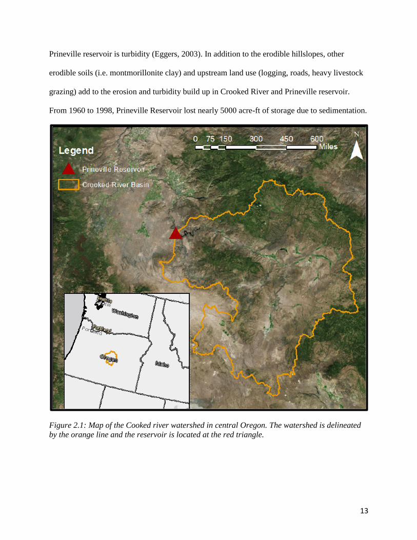
2003). The reservoir is fed by the 14133 km2 Crooked River watershed located in the Deschutes
River basin, a map of which is seen in figure 2.1. The Prineville region is in an arid climate with
hot dry summers and cold winters (Eggers, 2003). The Crooked River watershed averages 12
inches of rain per year, 90% of which falls between November and February. Winter
temperatures often fall below 0F (-18C) (January average is 32 F (0C)), while summers
rarely go above 100 F (38C) (July average is 60F (15.5C). The mean annual streamflow is
approximately 270,000 acre-feet/year (1 acre-foot = 1233.5 m3), ranging from 690,000 af/yr to
40,000 af/yr (Eggers, 2003).
The Crooked River watershed contains a variety of land cover types and diverse
geography. It is bordered by mountain ranges on the northern and south-central boundaries. The
southern region is comprised of mostly plains and grasslands (Gesch et al., 2002). The geology
of the watershed includes basalt, fine grain volcanic duff and lava flows. Over time, erosion
transformed the previously soft bed surrounding the reservoir to steep gullies. The reservoir is in
a shallow valley surrounded by steep hillsides, 90% of which are highly erodible soils. Due to
the highly erodible soils, the primary water quality concern for both the Crooked River and
13
Prineville reservoir is turbidity (Eggers, 2003). In addition to the erodible hillslopes, other
erodible soils (i.e. montmorillonite clay) and upstream land use (logging, roads, heavy livestock
grazing) add to the erosion and turbidity build up in Crooked River and Prineville reservoir.
From 1960 to 1998, Prineville Reservoir lost nearly 5000 acre-ft of storage due to sedimentation.
Figure 2.1: Map of the Cooked river watershed in central Oregon. The watershed is delineated
by the orange line and the reservoir is located at the red triangle.

14
2.2 Data Sources
The data sources for this study are summarized in table 2.1. They include
hydrometeorological data, soil and vegetation parameters, streamflow measurements and
reservoir volume surveys.
The hydrometeorological data used as inputs for the VIC model were developed by
(Livneh et al., 2015, 2013). The dataset provides daily maximum and minimum temperature,
windspeed and precipitation values. It is gridded for the Conterminous United States (CONUS)
on a 1/16° resolution. The soil texture values (more details on this will follow) are from survey
data, although some will be varied for a sensitivity analysis (Mill and White, 1998). The inputs
for VIC comprise of a variety of soil characteristics including infiltration, hydrologic
conductivity and maximum baseflow velocity.
Daily average streamflow observations came from U.S. Geological Survey (USGS) gage
14080500, Crooked River near Prineville, OR. Streamflow data from the USGS are available
from 1941 to 2018 and are not corrected for the influence of upstream reservoir intakes. The
USGS data were supplemented by the USBR Hydromet (hydrologic and meteorological
monitoring stations) historical dataset. In addition to streamflow, Hydromet includes naturalized
streamflow for post-dam construction flows in addition to uncorrected discharge flows. The
naturalized streamflow is reported as daily average flow starting in 1973 continuing to the
present, and discharge flows are available from 1941 to 2018.
Reservoir volumetric surveys collected by USBR were used to quantify volume loss in
Prineville Reservoir (Ferrari, 1999).There are two available surveys for Prineville collected in
1960 and 1998. The survey method used in 1998 was sonic depth recording interfaced with GPS
giving continuous sounding throughout the reservoir. The method used in the 1960 survey was

15
not specified, but it was likely the line and sinker method which was common at the time.
Notably, the limitation to reservoir surveys is that sediment density is often unknown. Sediment
density can range from 40-100 lb/ft3 with it most commonly falling between 60 and 80 lb/ft3.
Since the sediment survey data for Prineville lacks a density measurement, the entire range of
density is considered here.
Table 2.1: Data sources used for model inputs and model analysis
Data Type Dates Citation
Soil Parameters (Maurer et al., 2002)
Vegetation Parameters (Hansen et al., 2000)
Meteorology 1915 to 2015 (Livneh et al., 2015)
Streamflow 1941 to 2018 (U.S. Geological Survey, 2016)
Naturalized Flow 1973 to 2018 (U.S. Bureau of Reclamation, 2016)
Reservoir Volume June 1, 1960 and May 31
1998
(U.S. Geological Survey Water
Information Coordination Program,
2014)
2.3 Hydrologic Model and Sediment Algorithms
The sediment ensemble for this study was developed by Stewart et al., (2017). It consists
of five algorithms, three of which are hydrologically forced. In this study, we will be using the
three hydrologically forced algorithms which are outlined in the following sections. Important
parameters for these algorithms are described further in table 2.2.
2.3.1 Hydrologic Model – Variable Infiltration Capacity model
The Variable Infiltration Capacity model (VIC) will be used to model hydrologic
processes needed to drive the sediment algorithms (Liang et al., 1994). VIC is a widely used,
distributed hydrologic model that uses soil, vegetation and meteorological forcing inputs to
compute surface water and energy balances. For this application it is run on 1/16° (~ 6 km) grid
cells at a daily time step. The processes important to sediment yield include precipitation impact,
surface runoff and total streamflow.
16
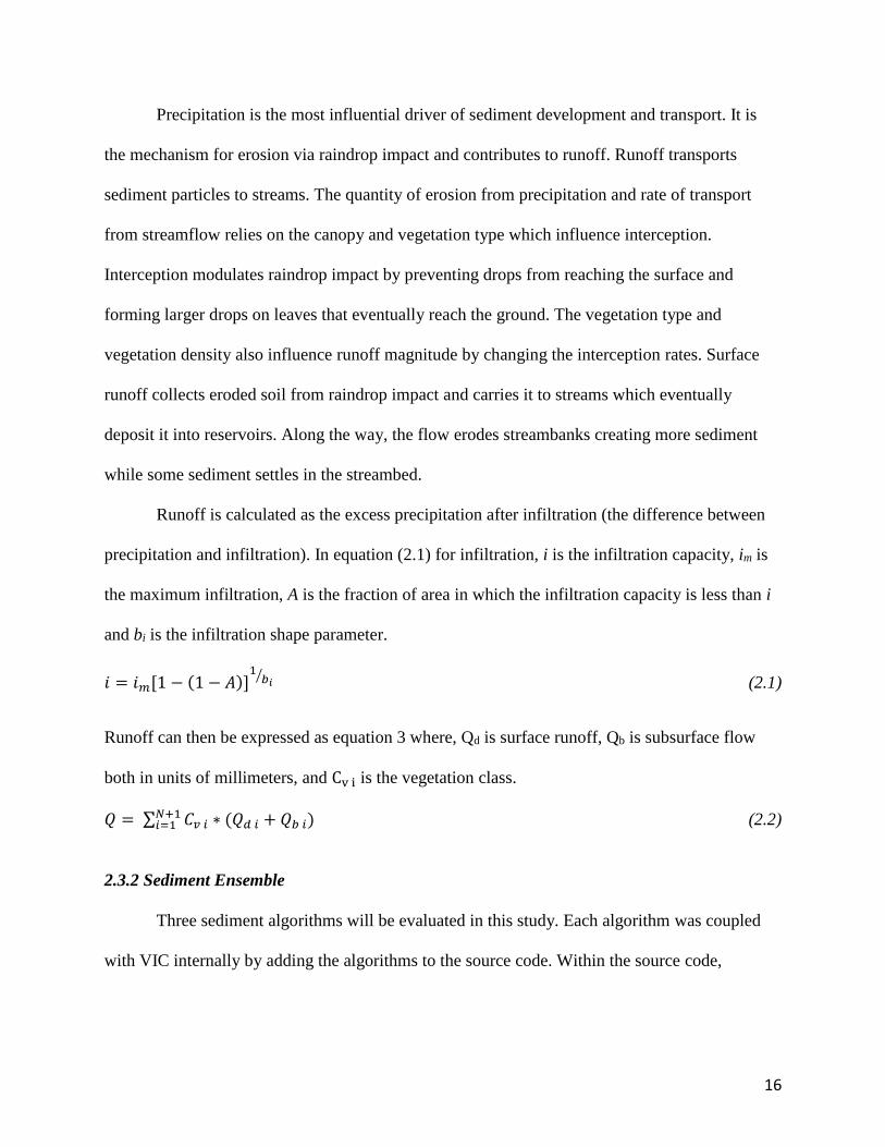
Precipitation is the most influential driver of sediment development and transport. It is
the mechanism for erosion via raindrop impact and contributes to runoff. Runoff transports
sediment particles to streams. The quantity of erosion from precipitation and rate of transport
from streamflow relies on the canopy and vegetation type which influence interception.
Interception modulates raindrop impact by preventing drops from reaching the surface and
forming larger drops on leaves that eventually reach the ground. The vegetation type and
vegetation density also influence runoff magnitude by changing the interception rates. Surface
runoff collects eroded soil from raindrop impact and carries it to streams which eventually
deposit it into reservoirs. Along the way, the flow erodes streambanks creating more sediment
while some sediment settles in the streambed.
Runoff is calculated as the excess precipitation after infiltration (the difference between
precipitation and infiltration). In equation (2.1) for infiltration, i is the infiltration capacity, im is
the maximum infiltration, A is the fraction of area in which the infiltration capacity is less than i
and bi is the infiltration shape parameter.
𝑖 = 𝑖𝑚[1 − (1 − 𝐴)]1
𝑏𝑖 ⁄
(2.1)
Runoff can then be expressed as equation 3 where, Qd is surface runoff, Qb is subsurface flow
both in units of millimeters, and Cv i is the vegetation class.
𝑄 = ∑ 𝐶𝑣 𝑖𝑁+1𝑖=1 ∗ (𝑄𝑑 𝑖 + 𝑄𝑏 𝑖) (2.2)
2.3.2 Sediment Ensemble
Three sediment algorithms will be evaluated in this study. Each algorithm was coupled
with VIC internally by adding the algorithms to the source code. Within the source code,

17
hydrologic variables such as precipitation, runoff and baseflow were applied explicitly to the
algorithms.
Modified Universal Soil Loss Equation
The Modified Universal Soil Loss Equation (MUSLE) is an empirical algorithm that uses
catchment characteristics to predict soil erosion based on the peak streamflow and total volume
of an event (Arnold et al., 1998). The average soil loss (A) is calculated from equation 2.3.
𝐴 = 𝑅𝐾𝐿𝑆𝐶𝑃 (2.3)
R is the runoff factor (see equation 2.4) which is calculated using the total runoff in an event
(𝑄, 𝑚𝑚) and peak streamflow rate of the event (qp, mm). When imbedded into VIC, qp was
defined as the max streamflow rate during a 24-hour time step. K is the soil erodibility index, LS
(m) is a topographical index for the length and steepness of the slope, C is a crop management
factor for vegetation and P is a landcover factor.
𝑅 = 11.8(𝑄 ∗ 𝑞𝑝)0.56 (2.4)
The MUSLE equation is limited by its assumption that the soil loss is linearly proportional to a
set of catchment characteristics. In addition, because it is an empirical algorithm many of the
inputs are not directly measured, hence they are difficult to determine.
Hydrological Simulation Program—Fortran
The Environmental Protection Agency (EPA) developed the Hydrological Simulation
Program – Fortran (HSPF) based on the Stanford Watershed Model (Bicknell et al., 1996;
Johanson et al., 1980). It is a conceptual algorithm that uses hillslope erosion algorithms for soil
detachment from rainfall and scour by overland flow. These processes were embedded into the
VIC framework. Rainfall detachment (𝐷𝐸𝑇,𝑡𝑜𝑛𝑠
𝑎𝑐/𝑖𝑛𝑡𝑒𝑟𝑣𝑎𝑙) considers the kinetic energy of

18
raindrops as seen in equation 2.5. 𝑑𝑡 is the number of hours in the time interval, 𝑅𝐶 is the
fraction of snow and vegetation cover, 𝑃 is the practice management factor from USLE (the
universal soil loss equation), 𝐾 is the detachment coefficient from USLE, 𝐼 (𝑖𝑛
𝑖𝑛𝑡𝑒𝑟𝑣𝑎𝑙) is the
rainfall intensity and 𝐽𝑅 is the detachment exponent.
𝐷𝐸𝑇 = (𝑑𝑡(1 − 𝑅𝐶)(𝑃)(𝐾)( 𝐼𝑑𝑡
))𝐽𝑅 (2.5)
To estimate SSL, HPSF uses transport capacity (TC, tons/ac/interval) in equation 2.6 where KS
is the transport coefficient, SU (in) is surface water storage, SO (in/interval) is surface water
outflow and JS is the transport exponent. The transport capacity represents the amount and size
of sediment that can be carried by the flow of water in a stream. The higher the flowrate, the
higher the transport capacity. As the transport capacity decreases, particles are deposited on the
streambed because settling velocity of some sediment particles is greater than the transport
capacity.
𝑇𝐶 = 𝑑𝑡(𝐾𝑆) (𝑆𝑈+𝑆𝑂
𝑑𝑡)
𝐽𝑆
(2.6)
The effect of the previous day’s rainfall on sediment production is simulated by decreasing DET
for days without a storm event. This is done with the AFFIX parameter in equation 2.7 which
increases each day due to soil compaction.
𝐷𝐸𝑇 = 𝐷𝐸𝑇(1.0 − 𝐴𝐹𝐹𝐼𝑋) (2.7)
A feature of HSPF is that it is relatively simple, as it uses concepts of physical
mechanisms to drive SSL generation. However, many of the coefficients and exponents are not
directly measurable and rely on calibration to estimate values. In turn, calibration relies on
observations. The nature of calibrating non-physically based parameters can lead to over fitting.

19
Systeme Hydrologique European Sediment Algorithm
The Systeme Hydrologique European Sediment algorithm (SHE-SED) (Wicks and
Bathurst, 1996) is a sediment transport scheme used within the Distributed Hydrology Soil
Vegetation Model (DHSVM) (Wigmosta et al., 1994). DHSVM is a physically based distributed
model that solves the energy and water balance equations. SHE-SED is the most complex of the
algorithms used in this study. DHSVM and SHE-SED rely on fine resolution vegetation and
topography, which causes limitations on large scale modeling efforts. The hillslope erosion
algorithms for overland flow and raindrop impact from the SHE-SED algorithm were embedded
into the VIC framework. By removing the SHE-SED algorithms from DHSVM, the algorithm no
longer includes the dynamic routing scheme DHSVM is known for which may influence its
performance. Henceforth, this algorithm will be referred to as DHSVM.
Overland flow detachment (Dof, m3/s/m) quantifies the sediment that is eroded by
overland flow. It is calculated by equation 4 where 𝛽𝑑𝑒 is the detachment coefficient, 𝑑𝑦 (m)is
the horizontal hillslope length, 𝑣𝑠(𝑚/𝑠) is the settling velocity, and TC (m3/m3) is the transport
capacity.
𝐷𝑜𝑓 = 𝛽𝑑𝑒(𝑑𝑦)(𝑣𝑠)(𝑇𝐶) (2.8)
Raindrop detachment is the erosion from raindrop impact. It is calculated as the momentum
squared of direct throughfall (MR) and leaf drip from vegetation (Md) from equations (2.9) and
(2.10) respectively. I (mm/hr) is rainfall intensity, and are coefficients from (Wicks, 1988), 𝑉
is leaf drip fall velocity, 𝜌 (𝑘𝑔/𝑚2/𝑠) is water density, 𝐷(𝑚) is leaf drip diameter, 𝐷𝑟𝑖𝑝 is the
percent of canopy drainage that falls from leaves and 𝐷𝑟𝑎𝑖𝑛 (𝑚/𝑠) is drainage from the canopy.
𝑀𝑅 = 𝛼𝐼𝛽 ( 2.9 )

20
𝑀𝑑 =(
𝑉𝜌𝜋𝐷3
6)
2
𝐷𝑟𝑖𝑝 𝐷𝑟𝑎𝑖𝑛
(𝜋𝐷3
6)
( 2.10 )
Critical Area Approach
Each model is applied on 1/16-degree VIC grid cells (~6 km). In large basins, (greater
than 500km2) 6 km grid cells provide an adequate resolution for modeling hydrology. However,
many erosion processes occur on the scale of meters. The spatial discretization needed to
quantify sedimentation is limited by computational power and available data at the scale of 6 km.
Instead, the critical area approach is used to quantify sediment development on individual
hillslopes that can then be upscaled to the larger VIC grid cells.
Critical areas are defined as the portion of the model grid cell that contributes to the
suspended sediment load, which is used to determine where soil erosion is most likely to occur.
In Stewart et al., (2017), critical areas were determined by using a threshold of slope steepness
and stream proximity. In this study, the critical area was included in the sensitivity analysis with
a range of values from 0 % to 100 % to determine the importance of estimating the critical area
accurately for reservoir sedimentation estimates.
Modeling Assumptions for Reservoir Sedimentation
Stewart et al., (2017), developed the sediment ensemble to include a routing scheme.
However, for the application to reservoir sedimentation, the timing of SSL is less important than
other applications, since we are primarily interested in sediment accumulation on longer
timescales (monthly to decadal) rather than the shorter timescales (hourly to daily) relevant to
water treatment. For this reason, the sediment routing scheme was not included in the present
application of the model ensemble. It is important to note that because sediment routing is not

21
included, the results presented here are only applicable to long-term (monthly to decadal)
sedimentation.
The second major assumption in comparing accumulated SSL with surveyed reservoir
sediment is that SSL comprises all loading into the reservoir. This assumption precludes
sediment from bedload which can be up to 10% of the total sediment yield. Therefore, for
drainages with large bedload this assumption will not be valid.
2.4 Sobol Sensitivity Analysis
The reservoir sedimentation estimates in this thesis are a new application of the multi-
algorithm sediment ensemble method developed by J. Stewart et al. (2017). To evaluate this new
application and to understand key sensitivities in modeling reservoir sedimentation, a Sobol
Sensitivity Analysis is performed, herein “Sobol”, (Sobol, 2001). Sensitivity analyses assist
modelers in identifying the importance of parameters for a desired output. The sensitivity
analysis for streamflow and sediment will be done independently. Stewart et al. (2017)
performed a joint calibration—a simultaneous calibration of both streamflow and sediment
parameters—but did not perform a sensitivity analysis. The best performing simulation from the
streamflow sensitivity analysis will be used to force the sediment ensemble. By isolating the
sensitivity analysis for the streamflow model from the sediment ensemble, it ensures the
streamflow inputs are as realistic as possible when used to drive the sediment ensemble. This is
important because sediment accumulation relies heavily on streamflow magnitude.
2.4.1 Theory
Sobol is a variance-based global sensitivity analysis which allows sampling of the entire
range of input parameters (Sobol, 2001). Sobol uses an ensemble of parameter realizations to
evaluate parameter influence on the variance. This study uses the Saltelli improvement of Sobol
22
which increases the efficiency by decreasing the number of parameter sets needed in the model
ensemble (Saltelli, 2002). From the variation in the ensemble of model outputs, Sobol produces
indices that that identify the fraction of the variance of the output that is influenced by a given
parameter or set of parameters and represent parameter sensitivity. The outputs used here are a
set of objective functions used to describe the skill of the streamflow model and sediment
algorithm outputs, relative to observations.
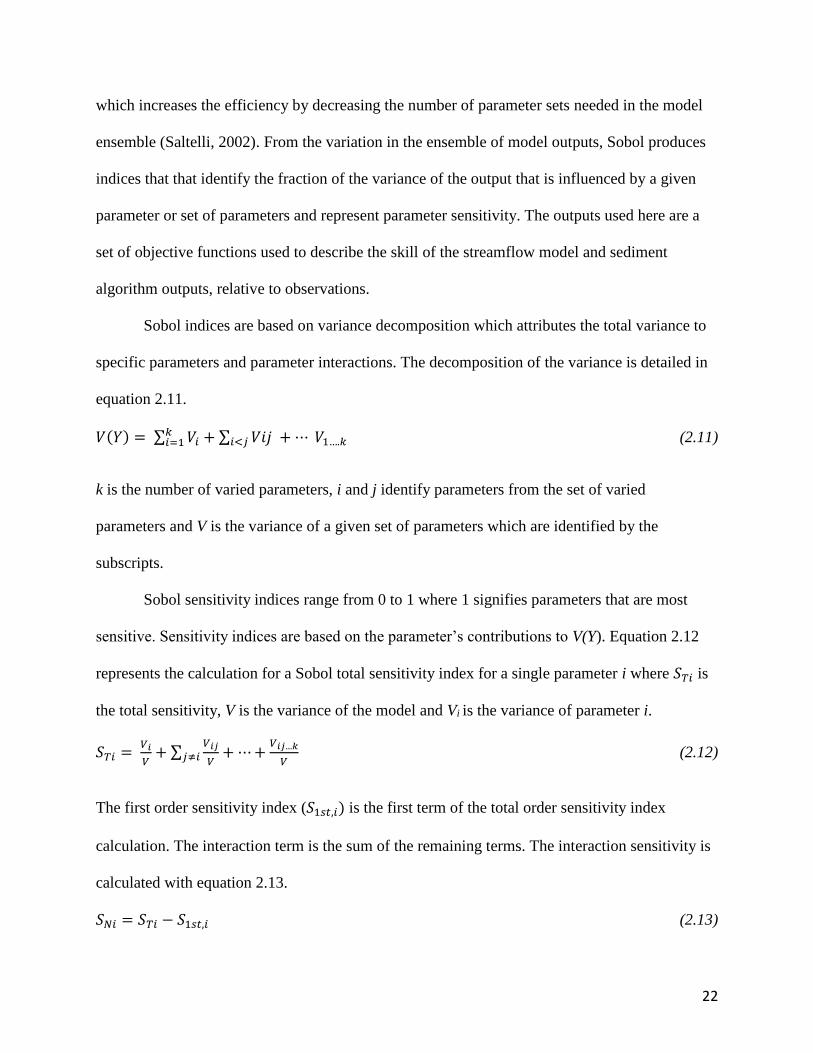
Sobol indices are based on variance decomposition which attributes the total variance to
specific parameters and parameter interactions. The decomposition of the variance is detailed in
equation 2.11.
𝑉(𝑌) = ∑ 𝑉𝑖𝑘𝑖=1 + ∑ 𝑉𝑖𝑗𝑖<𝑗 + ⋯ 𝑉1….𝑘 (2.11)
k is the number of varied parameters, i and j identify parameters from the set of varied
parameters and V is the variance of a given set of parameters which are identified by the
subscripts.
Sobol sensitivity indices range from 0 to 1 where 1 signifies parameters that are most
sensitive. Sensitivity indices are based on the parameter’s contributions to V(Y). Equation 2.12
represents the calculation for a Sobol total sensitivity index for a single parameter i where 𝑆𝑇𝑖 is
the total sensitivity, V is the variance of the model and Vi is the variance of parameter i.
𝑆𝑇𝑖 = 𝑉𝑖
𝑉+ ∑
𝑉𝑖𝑗
𝑉𝑗≠𝑖 + ⋯ +𝑉𝑖𝑗…𝑘
𝑉 (2.12)
The first order sensitivity index (𝑆1𝑠𝑡,𝑖) is the first term of the total order sensitivity index
calculation. The interaction term is the sum of the remaining terms. The interaction sensitivity is
calculated with equation 2.13.
𝑆𝑁𝑖 = 𝑆𝑇𝑖 − 𝑆1𝑠𝑡,𝑖 (2.13)

23
Typically, three sensitivity indices are used to evaluate a model: First order, total order
and interaction sensitivity indices. Consider a model that has output Z and inputs X and Y. The
variance of Z can be decomposed into the variance caused by changes in X (first order
sensitivity), the variance caused by changes in Y (first order sensitivity) and the variance caused
by the interaction between X and Y (interaction sensitivity). The total order variance of X is the
sum of the variance caused by changes in X and the variance caused by X when Y is also varied.
The total order variance of Y is the sum of the variance caused by changes in Y and the variance
caused by Y when X is also varied. With more than two parameters, the interaction variance can
be decomposed into second order, third order, fourth order, and so forth. For example, second
order variance is the variance caused by one parameter when two others are also varied.
Sobol uses a quasi-random sampling method similar to Latin hypercube sampling called a
Sobol sequence (Sobol, 1976). The Sobol sequence ensures that the global parameter space of
each parameter is evenly distributed. It does this by adding samples to the parameter space away
from previously established samples (Nossent et al., 2011). The samples produced from this
technique will be used to perform the Sobol sensitivity analysis.
2.4.2 Application
In simple models, the sensitivity of all parameters can be calculated. However, due to the
complex and computationally intensive nature of VIC and sediment ensemble, a subset of
parameters was selected to adhere to computational restraints. The parameters in table 2.2 were
chosen for the sensitivity analysis based on Stewart et al. (2017).
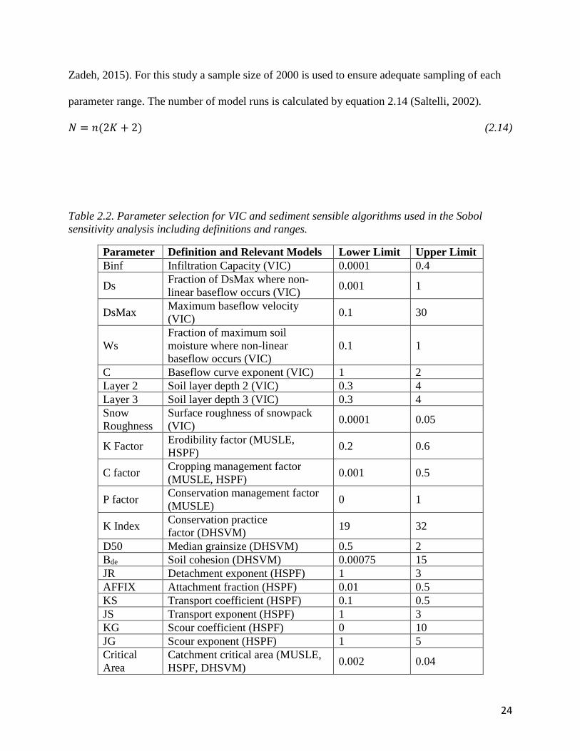
The number of model realizations depends on the number of parameters and the desired
sample size. For complex environmental models, sample sizes range between 1000 and 2000
(Houle et al., 2017; Nossent and Bauwens, 2012; Tang et al., 2007; van Werkhoven et al., 2008;
24
Zadeh, 2015). For this study a sample size of 2000 is used to ensure adequate sampling of each
parameter range. The number of model runs is calculated by equation 2.14 (Saltelli, 2002).
𝑁 = 𝑛(2𝐾 + 2) (2.14)
Table 2.2. Parameter selection for VIC and sediment sensible algorithms used in the Sobol
sensitivity analysis including definitions and ranges.
Parameter Definition and Relevant Models Lower Limit Upper Limit
Binf Infiltration Capacity (VIC) 0.0001 0.4
Ds Fraction of DsMax where non-
linear baseflow occurs (VIC) 0.001 1
DsMax Maximum baseflow velocity
(VIC) 0.1 30
Ws
Fraction of maximum soil
moisture where non-linear
baseflow occurs (VIC)
0.1 1
C Baseflow curve exponent (VIC) 1 2
Layer 2 Soil layer depth 2 (VIC) 0.3 4
Layer 3 Soil layer depth 3 (VIC) 0.3 4
Snow
Roughness
Surface roughness of snowpack
(VIC) 0.0001 0.05
K Factor Erodibility factor (MUSLE,
HSPF) 0.2 0.6
C factor Cropping management factor
(MUSLE, HSPF) 0.001 0.5
P factor Conservation management factor
(MUSLE) 0 1
K Index Conservation practice
factor (DHSVM) 19 32
D50 Median grainsize (DHSVM) 0.5 2
Βde Soil cohesion (DHSVM) 0.00075 15
JR Detachment exponent (HSPF) 1 3
AFFIX Attachment fraction (HSPF) 0.01 0.5
KS Transport coefficient (HSPF) 0.1 0.5
JS Transport exponent (HSPF) 1 3
KG Scour coefficient (HSPF) 0 10
JG Scour exponent (HSPF) 1 5
Critical
Area
Catchment critical area (MUSLE,
HSPF, DHSVM) 0.002 0.04

25
K is the number of parameters, n is sample size and N is the total number of model runs. The
sensitivity analysis for stream flow includes 8 parameters resulting in 36,000 parameter
realizations. The analysis for sediment includes 13 parameters, thus resulting in 60,000
realizations.
2.5 Model Performance Measures
The streamflow model and sediment ensemble sensitivities are evaluated using objective
functions. Selecting appropriate objective functions is important because each objective function
emphasizes specific aspects of the behavior of the model (McCuen et al., 2006). They were
selected from common hydrologic objective functions that address aspects important for
sediment estimates. They are detailed in equations 2.15 to 2.21. For the following equations S is
the simulation, O is the observation, N is the number of observations and i corresponds to an
observation or simulation at a specific moment in time. The objective functions used here are
NSE for overall fit, RMSE for overall error, R for timing errors, ratio of the variance for
variability and percent bias for systematic biases.
In a subsequent analysis, RMSE was also used to evaluate the extent to which the
sediment algorithms predict sediment accumulation that differs from the traditional linear
assumption. Finally, the amount of sediment accumulation from the first half of the model
simulation to the second half of each model simulation was compared with a percent difference.
Nash Sutcliffe Efficiency
The Nash Sutcliffe Efficiency (NSE; Nash and Sutcliffe, 1970) was developed for
specific use in hydrology and has become a commonly used objective function in the field
(Gupta et al., 2009). The calculation, provided in equation 2.15, includes components of

26
correlation, bias and variability. NSE values range from -∞ to 1, with 1 being a perfect match
and 0 being that the simulations do an equivalent job of matching the observations as the mean
of the observations.
𝑁𝑆𝐸 = 1 − ∑ (𝑆𝑖− 𝑂𝑖)2𝑁
𝑖=1
∑ (𝑂𝑖− 𝑂)2𝑁𝑖=1
(2.15)
NSE is sensitive to a number of factors, including sample size, outliers, magnitude bias, and
time-offset bias (McCuen et al., 2006). One of the main concerns about NSE is its use of the
observed mean as baseline, which can lead to overestimation of model skill for seasonally driven
variables such as runoff in snowmelt dominated basins (Gupta and Kling, 2011).
Pearson Correlation Coefficient
The Pearson correlation coefficient (R) helps determine if a positive or negative linear
relationship is present. It ranges from -1 to 1, with 1 being an exact positive relationship and -1
being an exact negative relationship. One drawback to the R metric is that it only measures linear
relationships and can be easily skewed by outliers. R is calculated by equation 2. 16.
𝑅 = ∑ (𝑆𝑖−𝑆𝑁
𝑖=1 )(𝑂𝑖−𝑂)
√∑ (𝑆𝑖−𝑆)2𝑁𝑖=1 ∑ (𝑂𝑖−𝑂)2𝑁
𝑖=1
(2. 16 )
Ratio of Variances
The ratio of variances is a comparison between the variance of modeled and observed
data. It ranges from 0 to ∞ with an optimal value of 1 signifying the variances are equal. Values
near 1 indicate high model skill. In terms of streamflow, a value near one would tell us that the
model and observations agree on extreme low and high flows. A value near zero indicates the
model has high peak and the observations have low peaks where as a value near infinity would

27
indicate the opposite. The variance is shown in equation 2.17 and the ratio of the variances in
equation 2.18 .
𝜎2 = ∑ (𝑋𝑖−𝑋)2𝑁
𝑖=1
𝑁 (2.17)
𝑉𝑎𝑟𝑖𝑎𝑛𝑐𝑒 𝑟𝑎𝑡𝑖𝑜 = 𝜎𝑠
2
𝜎𝑜2 (2.18)
Percent Bias (PBIAS)
Percent bias is a measure of systemic error. It measures the degree which the model
provides values above or below observed (Maidment, 1993). More simply, percent bias is the
difference in the accumulation of the model output and observations. Theoretically, values can
range from -∞ to ∞ with an optimal value of 0%. Negative values are underestimations and
positive values are over estimations. Percent bias is calculated with equation 2.20.
𝑃𝐵𝐼𝐴𝑆 = 100 ∑ (𝑆𝑖−𝑂𝑖)𝑁
𝑖=1
∑ 𝑂𝑖𝑁𝑖=1
(2.19)
Percent bias is helpful in hydrology because it can determine the quantitative difference in the
modeled values and observed values over extended time periods (Boyle et al., 2000). It is
applicable for reservoir sedimentation because accuracy over many years (5-20 or more) is
especially important for reservoir management.
Root Mean Squared Error
Root mean squared error (RMSE) is the standard deviation of the residuals for a predicted
value (modeled) and a known value (observed). Smaller values signal better model performance
with zero being perfect. There is no upper limit to the value of RMSE. RMSE is calculated with
equation 2.20.
𝑅𝑀𝑆𝐸 = √1
𝑁∑ (𝑆𝑖 − 𝑂𝑖)2𝑁
𝑖=1 (2.20)

28
2.6 Sediment Yield Linearity
A major goal of this research is to assess the validity of assuming linear sediment yield.
To this end, we chose a set of “behavioral” simulations that provide probable estimates of
sedimentation. Although there exist two sediment volume surveys for Prineville Reservoir, the
sediment density is unknown. Therefore, instead of having a single known value of volume loss,
we have a range of possible sediment volume loss, governed by the sediment density range of 40
-100 lb/ft3, which is the full range of sediment densities. In future studies a narrower sediment
density range could be used. We use this information to choose behavioral simulations, defined
as the set of model realizations that have their final accumulated sediment volumes falling within
the density range.
To evaluate the relative yield linearity of each sediment algorithm we employ an RMSE
calculation that can be considered the “Root Mean Squared Difference” between modeled
sediment yield and the simple linear yield assumption of constant accumulation through time.
Because the root mean squared difference equation is functionally equivalent to the classic
RMSE equation, the term RMSE will be used, although the values are not considered “errors”
necessarily since the exact sediment density is unknown. Specifically, the RMSE will be
calculated for yearly sediment accumulation between the modeled yearly accumulation and the
linear assumption accumulation. Then the reported RMSE is the difference in the yearly average
between the sediment algorithm and the linear yield assumption. Moreover, the RMSE values
will also be expressed as a percentage difference, showing how the accumulated differences
between modeled sedimentation compares to the linear sedimentation estimates. The percent
difference will simply be the yearly RMSE for a given model divided by the linear yearly
sediment accumulation for a given simulation realization.

29
A final consideration in this analysis is how to calculate the assumed linear yield rate.
Broadly, the yield linearity assumption is essentially a monotonic accumulation beginning at
zero on the day of the first reservoir survey and ending at the value of modeled sediment
accumulation on the day of the final reservoir survey. Thus, the linear yield estimate is
dependent on the final sedimentation accumulation, which is not strictly known. Rather than
compare simulated sediment accumulation to a single linear function, which would assume a
known sediment density, each simulation is compared to a different linear yield rate equation
based on the final modeled sediment accumulation value.
The second method used to determine yield linearity is a comparison of sediment
accumulation between two time periods. The simulation spans 1960 to 1998 which will be split
into time period 1 (1960 to 1979) and time period 2 (1979 to 1998). The accumulated sediment
for these 19-year spans will be compared with a percent difference for each simulation.

30
Chapter 3: Results
Overview
The results are discussed in the following three sub-sections. First, the sensitivity analysis
and parameter selection for streamflow are presented. This is followed by the sensitivity analysis
and parameter investigation for the sediment ensemble. For each analysis, the sediment ensemble
results are presented in the following order: MUSLE, HSPF, DHSM. Finally, there is an
evaluation of the yield linearity of each sediment algorithm.
3.1 Streamflow Sensitivity
The sensitivity analysis for VIC streamflow was performed on modeled streamflow from
1975 to 1998 to match the available naturalized flow data after reservoir construction. Figure 3.1
shows the results of the sensitivity analysis. Sobol sensitivity indices range from 0 (white)
indicating no sensitivity, to 1 (dark purple) with 1 indicating the most sensitivity. Each square in
the matrix represents the sensitivity of a parameter for a single objective function.
Figure 3.1: First order sensitivity, second order sensitivity and interaction for streamflow
objective function from VIC. Dark colors represents more sensitive parameters.

31
Demaria et al., (2007) used a Monte Carlo sensitivity analysis to find that layer 2 and binf
were sensitive parameters for VIC streamflow. There is broad agreement that streamflow is
sensitive to changes in layer 2 with a strong first order sensitivity. However, in contrast to
Demaria et al. (2007) binf—the infiltration capacity of the soil—appears to be insensitive in this
analysis. The streamflow’s minimal sensitivity to binf can be explained by the Crooked River
watershed’s arid climate, with only 11 inches of precipitation per year. For the Crooked River
watershed, infiltration is controlled by the amount of runoff. Even if there is a high infiltration
capacity, there is a limit to the amount of runoff available to infiltrate into the soil. Based on the
VIC model simulations, the Crooked River is assumed to be driven primarily by baseflow. This
assumption comes from the model runoff to baseflow ratio from 1960 to 1998 (years of sediment
volume surveys) is 0.38, showing that there is more than twice the volume of baseflow than
runoff, as illustrated in figure 3.2b. Figure 3.2a shows that the yearly modeled accumulated
streamflow and peak snow pack are similar values in most years, so the majority of streamflow
develops as snowmelt, not runoff from precipitation.
Interaction sensitivity is the product of the variance produced by changing two or more
parameters simultaneously. The sensitivity analysis for VIC shows little interaction sensitivity
relative to first order sensitivity for layer 2. Ds and Dsmax show more interaction sensitivity
compared to first order sensitivity for the ratio of variances, RMSE, percent bias and NSE.
However, they show less sensitivity in correlation, R. R and Ratio of Variances have more
sensitivity to parameter interaction than RMSE, percent bias and NSE.

32
a)
b)
Figure 3.2: a) Yearly maximum snowpack (SWE) and yearly accumulative streamflow (runoff
and baseflow) from 1960 to 1998. b) Runoff and baseflow accumulation from date of the first
reservoir volume survey to the date of the final reservoir volume survey. Data for both panels
come from VIC simulations.
3.2 Streamflow Model Selection
The streamflow parameters that would be used to drive VIC were selected from the
model instances used for the Sobol sensitivity analysis. The initial results from the model
realizations used in the Sobol sensitivity analysis revealed discrepancies between the modeled
and the observed streamflow. Typically, an NSE greater than 0.5 is desirable for streamflow.
However, past studies found the Crooked River watershed challenging to model. Mendoza et al.,
(2017) found a best NSE of 0.34 for fully calibrated SAC- SMA (Sacramento Soil Moisture
Accounting) model. A USBR study also found poor model performance for the Crooked River
Basin (Turner, 2011). They used VIC and found a maximum R2 value of 0.3. The primary
concern for this study, where sediment is being mobilized, is that the peak flow magnitude and
timing should match. An example is seen in figure 3.3, where the model struggles to produce
these features, which is consistent with the aforementioned past studies.

33
A key modification was explored to improve the model result, namely the snow albedo
parameters were adjusted because snowmelt is a key factor driving peak flow timing and
magnitude. Notably, this modification occurred outside the usual set of soil parameters that are
adjusted during calibration, i.e. this is a ‘hard-coded’ parameter. We following the guidance of
past studies that highlighted the importance of modifying hard-coded parameters (Houle et al.,
2017; Mendoza et al., 2017). The second round of Sobol simulations, resulted in much improved
streamflow, shown in Figure 3.3. below. The best results had an NSE around 0.28 and a R less
than 10%, which are comparable to those by Mendoza et al. (2017) and Turner et al. (2011).
Figure 3.3: Monthly observed and modeled streamflow. The black line is the naturalized
observed flow and the colored lines are model realizations. The blue line shows the model
streamflow from the default albedo parameters. The red line shows the model streamflow from
adjusted albedo parameters.
Table 3.1:a) Objective functions for the top performing streamflow parameters b)Parameters
used to drive streamflow for the sediment ensemble
a)
NSE % Bias Var/Var R
0.282 6.8 0.408 0.541
b)
Binf Ds Ds max Ws C Layer 2
Depth
Layer 3
Depth
Snow
roughness
0.0948 0.0040 10.93 0.910 1.44 0.997 3.59 0.043
The Sobol sensitivity analysis produced 40,000 model realizations of VIC streamflow.
This number of realizations, together with comparable performance with past studies, gave us
confidence that we had sufficiently sampled model space to select a set of streamflow parameters

34
that would force the sediment ensemble as realistically as possible. The selected model
realization had a percent bias of 6.8 and an NSE of 0.28 (see table 3.1a for all objective
functions). Despite the low NSE, visual inspection shows that the model captures key features of
the hydrograph reasonably well. The obvious issue is that the model severely underestimates
peaks in 1985, 1986, 1989 and 1993. However, for other years the model matched the peak
streamflow magnitude and timing to a satisfactory level. The selected parameters are in table
3.1b.
The assumption for the following sediment results is that VIC realistically models
streamflow. First, the assumption is that VIC correctly partitions the total streamflow between
baseflow and runoff. This is especially important because the sediment algorithms rely, to
varying degrees, on the quantity of baseflow. The biases in the simulations of the VIC model
variables, specifically runoff and baseflow will carry through the modeling process and impact
sediment yield since the yield computation is driven by these hydrologic variables. The second
assumption is that the soil and vegetation parameters did not change over time, i.e. static
vegetation and soil parameter were used and would not account for alterations from
development, agriculture, soil compaction, etc.
3.3 Reservoir Sediment Accumulation
The streamflow parameters selected through the model realizations used for the Sobol
sensitivity analysis were used to drive the sediment ensemble. Sediment results are presented
assuming that 100% of the sediment yielded by each algorithm will accumulate as reservoir
sediment, e.g. a 100% trap efficiency. The model results, in kg, are compared to reservoir
volume surveys measured in acre-feet. To convert the model output and observations to common
units an assumption of sediment density was needed. Sediment density can range from 40-100

35
lb/ft3. Range from the maximum to minimum sediment weight will be referred to as the sediment
density error bars. The subset of model realizations with total accumulated sediment that falls
within the sediment density error bars are considered ‘behavioral samples’ that are used to
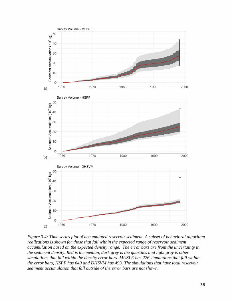
analyze the algorithms predicted reservoir sediment accumulation and sensitivity patterns. Figure
3.4 shows the behavioral subsets for each algorithm in the sediment ensemble. All three
algorithms are driven partially by precipitation; the models differ in how they consider baseflow
and runoff in the sedimentation equations.
The results for MUSLE are seen in figure 3.4a. MUSLE is an empirical algorithm that
uses catchment characteristics and peak streamflow to determine sedimentation. Unlike the other
algorithms that rely exclusively on surface runoff, MUSLE is driven by total streamflow
(baseflow and runoff). The reservoir sediment accumulation pattern is driven by seasonal
oscillations in baseflow because the watershed is baseflow dominant. The yearly jumps signal
the algorithm’s ability to capture the seasonal oscillation in reservoir sediment accumulation.
Baseflow accumulation is depicted in figure 3.2. In addition, there are changes in yearly
reservoir sediment accumulations signified by the changes in slope between 1978 and 1985.
36
a)
b)
c)
Figure 3.4: Time series plot of accumulated reservoir sediment. A subset of behavioral algorithm
realizations is shown for those that fall within the expected range of reservoir sediment
accumulation based on the expected density range. The error bars are from the uncertainty in
the sediment density. Red is the median, dark grey is the quartiles and light grey is other
simulations that fall within the density error bars. MUSLE has 226 simulations that fall within
the error bars, HSPF has 640 and DHSVM has 493. The simulations that have total reservoir
sediment accumulation that fall outside of the error bars are not shown.

37
The results for HSPF are seen in figure 3.4b. HSPF is a runoff driven algorithm that
solves the energy and water balance equation to calculate sedimentation. The similarities
between HSPF and runoff can be seen in comparison to figure 3.4b and 3.2
The results for DHSVM are in figure 3.4c. There is some seasonal variation, but less
than in MUSLE. The DHSVM realizations from Sobol, under estimate the reservoir sediment
accumulation by a minimum of 30%. This poor performance is potentially because DHSVM was
originally developed for hydrologic modeling in forested mountain regions, and the Crooked
river basin is mostly flat grasslands. Furthermore, the DHSVM sediment physics are typically
coupled with dynamic routing, which was not included here. A more holistic analysis into model
physics would be required to address this issue in greater detail.
3.4 Sediment Sensitivity Analysis
To learn more about the processes behind the sediment development in each algorithm,
we turn to a Sobol sensitivity analysis. Each algorithm relies on different parameters, so each
algorithm has a different number of commonly calibrated parameters. Parameters chosen for the
sensitivity analysis were selected from Stewart et al., (2017) resulting in nine parameters for
HSPF, four for DHSVM and four for MUSLE1. The sensitivity analyses are presented in bar
graphs in figure 3.5. In addition to the sensitivity analysis results, dotty plots and parameter
distribution histograms are presented. The dotty plots show the relationship between the
objective function (percent bias) used for algorithm evaluation and parameter changes.
1 The results for MUSLE are not included because there were numerical errors in some model realizations, so the sensitivity analysis was not completed.

38
HSPF is more sensitive to parameter interactions than individual parameter changes. JG
has the most first order sensitivity, but it is still less than its interaction sensitivity. JG and critical
area have a high interaction index as well as JG and KG.
Figure 3.5: Bar graphs of Sobol sensitivity index values for DHSVM and HSPF. A value of one
signals most sensitive, and zero signals no sensitivity.
DHSVM has high first order sensitivity of D50 and critical area. In addition, both
parameters have a small amount of interaction sensitivity. Critical area is the percent of the area
that contributes sediment to the outflow. The fraction ranges from 0% to 100%, with typical
values falling between 30% and 100%. It is applied as a multiplier of the final sediment amount,
so the results from the algorithm rely heavily on critical area.
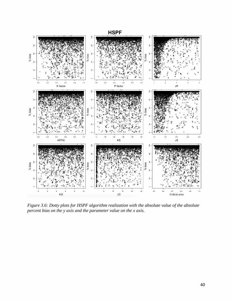
3.5 Dotty Plots
Dotty plots are useful to see patterns in parameter sensitivities when comparing objective
function for a range of parameter values (Wagener and Kollat, 2007). For example, they can be

39
used to diagnose the behavioral ranges of a parameter, relative to a given objective function. In
figure 3.6 and 3.7 the objective functions are on the vertical axis and the parameters are on the
horizontal axis. When a dotty plot shows a relatively uniform distribution of points with respect
to the vertical axis, this can be interpreted as little-to-no model sensitivity of the objective
function to the given parameter. When a pattern emerges, the objective function is sensitive to
changes in the parameter.
The dotty plots for HSPF are shown in figure 3.6. There is a similar exponential pattern
for JS and JR parameters suggesting high algorithm sensitivity. JS and JR are scour and
detachment exponents respectively. It is their application as an exponent that is seen in the dotty
plot. There is also a slight exponential pattern in JG. The patterns exhibited on the dotty plots for
the other parameters suggests a low amount of sensitivity. This agrees with the Sobol Sensitivity
analysis.
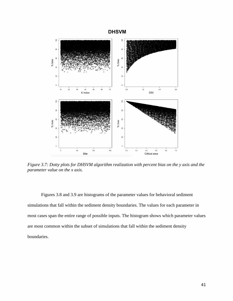
The dotty plots for DHSVM are seen in figure 3.7. None of the simulations had percent
bias below 30%. Critical area shows a distinct cutoff of objective function performance
compared to the value of critical area. This is an expected pattern because the critical area is the
percent of the catchment that is considered to contribute to sedimentation. As the critical area
decreases the minimum percent bias will move farther from zero. The sensitivity would not be as
strong if DHSVM generally underestimates sedimentation. The dotty plot for D50 (median
grainsizes) shows the sensitivity in the form of algorithm performance cutoff as well. The cutoff
here manifests from the grainsize because the grainsize influences the overland flow transport
capacity.
40
Figure 3.6: Dotty plots for HSPF algorithm realization with the absolute value of the absolute
percent bias on the y axis and the parameter value on the x axis.
41
Figure 3.7: Dotty plots for DHSVM algorithm realization with percent bias on the y axis and the
parameter value on the x axis.
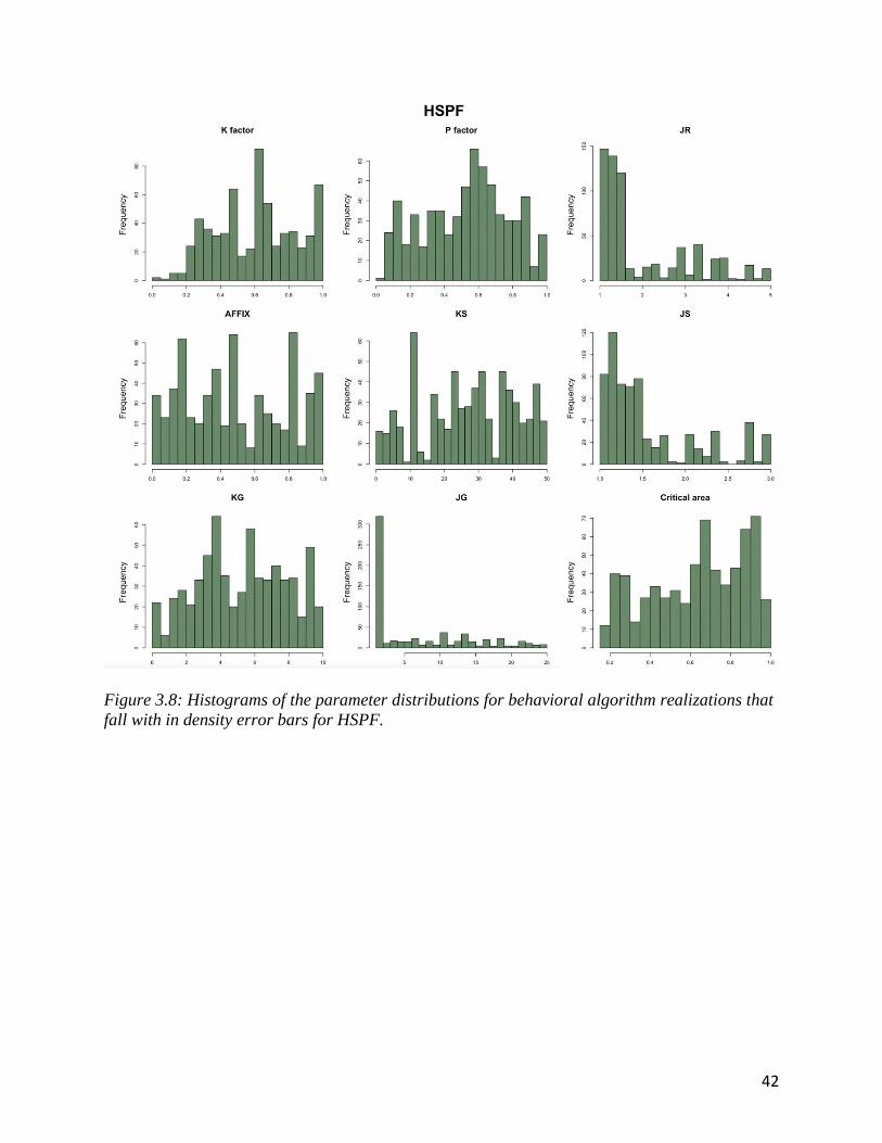
Figures 3.8 and 3.9 are histograms of the parameter values for behavioral sediment
simulations that fall within the sediment density boundaries. The values for each parameter in
most cases span the entire range of possible inputs. The histogram shows which parameter values
are most common within the subset of simulations that fall within the sediment density
boundaries.
42
Figure 3.8: Histograms of the parameter distributions for behavioral algorithm realizations that
fall with in density error bars for HSPF.
43
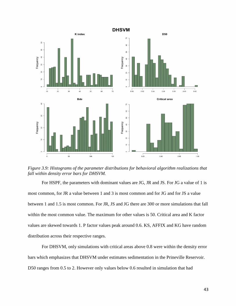
Figure 3.9: Histograms of the parameter distributions for behavioral algorithm realizations that
fall within density error bars for DHSVM.
For HSPF, the parameters with dominant values are JG, JR and JS. For JG a value of 1 is
most common, for JR a value between 1 and 3 is most common and for JG and for JS a value
between 1 and 1.5 is most common. For JR, JS and JG there are 300 or more simulations that fall
within the most common value. The maximum for other values is 50. Critical area and K factor
values are skewed towards 1. P factor values peak around 0.6. KS, AFFIX and KG have random
distribution across their respective ranges.
For DHSVM, only simulations with critical areas above 0.8 were within the density error
bars which emphasizes that DHSVM under estimates sedimentation in the Prineville Reservoir.
D50 ranges from 0.5 to 2. However only values below 0.6 resulted in simulation that had

44
accumulated sediment with in the density error bars. Only D50 below 0.6 performed within
reasonable bounds, this makes sense that it is the lower side because smaller grainsizes are able
to be transported more easily.
3.6 Linear Reservoir Sediment Accumulation Analysis
3.6.1 Root Mean Squared Difference
The assumption that sediment accumulates linearly through time in reservoirs has been
made in multiple past studies (Graf et al., 2010). To evaluate this assumption for the Prineville
Reservoir, RMSE was calculated for yearly reservoir sediment accumulation between each
algorithm realization and a comparable linear assumption with identical initial and final
accumulated sediment values. (See section 2.6 for clarification.) While the term RMSE is used,
we are effectively concerned in the Root Mean Squared Difference to characterize the deviation
between each algorithm and a linear assumption of reservoir sediment accumulation, rather than
to discuss error. Figure 3.10. shows histograms for each algorithm of yearly RMSE and table 3.1
conveys the deviation between the linear estimate and simulation as a percent of the linear
estimate. Only behavioral simulations are included in this analysis.
Table 3. 2: Percent yearly deviation from a linear assumption of reservoir sediment
accumulation for each of the three sediment algorithms.
Algorithm % yearly deviation
MUSLE 89.41 %
HSPF 24.32 - 41.52 %
DHSVM 45.07 %

45
Figure 3.10: Histograms of the yearly average RMSE for comparison to a linear assumption of
reservoir sediment accumulation. Smaller values indicate the simulation more similar to a linear
assumption. The values represent the average sedimentation error over the period from 1960 to
1998. MUSLE has 226 data points, HSPF has 640 and DHSVM has 493.

46
MUSLE has the largest yearly deviation from the linear assumption at 89.41% which is
followed by a 45.07% deviation for DHSVM. MUSLE and DHSVM have a small range of
RMSE for their respective algorithm simulation; the values are equivalent with each other to 5
decimal places and will hereafter be referred to as the same value. The values are the same across
the simulation for two reasons. First, the yield linearity analysis presented here assumes that each
respective simulation results in the correct amount of reservoir sediment accumulation by the end
of the run, meaning that each model simulation has a different linear function, specific that that
simulations initial and final value. Secondly, the parameters varied for the Sobol analysis in
MUSLE and DHSVM are linearly related to the resulting reservoir sediment accumulation.
Importantly, HSPF exhibited the most complex parameter interactions among the three
algorithms (Figure 3.5). The two most sensitive parameters were the scour and detachment
coefficients. These coefficients are applied as exponents, so are not linearly related to the
resulting reservoir sediment accumulation. Therefore, the HSPF simulations exhibit varying
degrees of deviation from the linear assumption of reservoir sediment accumulation, resulting in
a range in the percent difference. The relative RMSE for HSPF, 24.32 - 41.52 %, is the lowest of
the three algorithms.
When compared to the timeseries plots in 3.4, the difference from the linear estimate
agrees with the results. MUSLE, which is driven by both baseflow and runoff, shows the least
yield linearity because of the seasonal variation in streamflow. DHSVM and HSPF however are
driven by runoff which is limited in the Crooked River basin. They both produce sediment that
accumulates at a more constant rate than MUSLE.
In conclusion, these results demonstrate that the yield linearity of sediment is reliant on
the streamflow regime. When modeling these processes, it is important to note how each process
47
is incorporated into the sediment algorithms. For example, MUSLE accounts for total
streamflow, so the both baseflow and runoff influence its sediment yield, whereas HSPF and
DHSVM are exclusively driven by runoff. The simulated runoff in the Crooked River has a
relatively steady rate, such that DHSVM and HSPF appear to have a more linear sediment yield
than MUSLE.
3.6.2 Error Extrapolating Linear Projections
This section provides a comparison of sediment yield between the first 19 years and the
second 19 years of the time period between the reservoir surveys in 1960 and 1998. We attempt
to replicate linear yield estimates by treating the accumulated sediment yield value in 1979 as a
reservoir survey. The linear slope from the first period 1960-1979 is extended to the second
period 1979 to 1998 and an error between this extrapolation and the simulated value is calculated
as a percent difference. The percent difference for each model is seen in table 3.3. Figure 3.11
shows histograms of the total sediment yield for each simulation in the respective time periods,
1960 to 1979 on the left in yellow and 1979 to 1998 on the right in green.
The results are similar to the results from the root mean squared error yield linearity
assessment in section 3.6. It shows that the MUSLE simulations have the same percent
difference, likely due to the linear relationship between the varied parameters and the sediment
output. The DHSVM simulation also has the same percent difference because the parameters that
are changed for the sensitivity analysis linearly influenced the sediment output. The simulations
from HSPF, however, have a range of percent differences which show parameters in HSPF
influence the magnitude of sediment yield rate.

48
Figure 3.11: Total sediment yield for 1960 to 1979 (yellow) and 1979 to 1998 (green). Only
behavioral simulations with a final total sediment yield that fell within the sediment density error
bars as seen in figure 3.4 were analyzed.
Table 3.3: Percent difference between the total sediment yield from 1960 to 1979 and 1979 to
1998.
Algorithm Difference
MUSLE 164.17%
HSPF 11.9% to 34.00%
DHSVM 11.84%

49
Chapter 4 Discussion & Conclusion
Overview
As reservoir infrastructure in the United States continues to age, fill with sediment and be
stressed by climate change, it is increasingly important to understand the processes behind
sedimentation. The available reservoir volume surveys are too infrequent for understanding
climate-driven changes in sedimentation rates. Hydrologically forced algorithms offer a way to
inform process-level understanding of sedimentation drivers. Yet, few sediment algorithms have
been applied to the problem of reservoir sedimentation and an ensemble of algorithms have
hitherto not been brought to bear on this problem. We applied the hydrologically forced sediment
algorithm ensemble developed by Stewart et al., (2017) that includes physically-based,
conceptual, and empirical algorithms, to the Crooked River watershed which feeds Prineville
Reservoir near Bend, OR. Through a Sobol sensitivity analysis we aimed to address the
following questions:1) Can hydrologically-forced sediment algorithms help us advance reservoir
sedimentation estimates to improve future planning?2) To which processes and inputs are
reservoir sedimentation estimates most sensitive?
3) What can we learn from hydrologically driven algorithms that the linear sediment yield
assumption fails to assess?
4.1 Streamflow Sensitivity
Parameter sensitivity for streamflow within the VIC model was evaluated with a Sobol
sensitivity analysis. We found the layer 2 depth parameter was much more sensitive than other
parameters which was consistent with findings of Demaria et al., (2007). The basin’s gradual

50
snowmelt produces consistent low flows, therefore the limiting factor of infiltration is the
quantity of water, not the infiltration capacity (binf). For future modeling of arid, snowmelt
dominated basins the most important parameters are baseflow related. In the case of VIC, the
layer 2 depths need to be carefully calibrated.
4.2 Streamflow Selection
Streamflow parameters to drive sedimentation were chosen based on objective function
performance of the Sobol simulations. Initial results had poor peak flow performance for both
magnitude and timing. To improve this, snow albedo parameters were adjusted. The selected
parameters produced streamflow with NSE of 0.28 and a percent bias of 6.8%. Typically, for
streamflow, an NSE greater than 0.5 is desired. However, the Crooked River is known to be
challenging to model and our results are comparable to past studies (Mendoza et al., 2017;
Turner, 2011). Most importantly, the need to change snow parameters corroborates with Houle et
al., (2017) and Mendoza et al., (2015) who put forward that snow parameters are often fixed
which limits model performance. They suggested that hydrologic models should have snow
parameters that are easily adjusted to improve model performance.
4.3 The Linear Sediment Yield Assumption
The analysis of the difference between a linear yield assumption and the algorithms
indicated that errors associated with the yield linearity assumption can range from ±25- 90%
annually, depending on the chosen algorithm. MUSLE and DHSVM had differences from the
linear assumption of 89.4% and 45.1%, respectively. The parameters changed in the sensitivity
analysis for DHSVM and MUSLE have a linear relationship to the sediment output which results
in a commensurate difference for all simulations for the respective algorithms. However, HSPF
exhibited more complex parameter interactions and the most sensitive parameters (the scour

51
coefficient and detachment coefficient) are applied as exponents. The result is that the rate of
sediment yield is extremely sensitive to the value of the scour coefficient and detachment
coefficient parameters. This indicates that great care must be taken in identifying their values for
any applications of the sediment algorithms.
4.4 Future Work
This study investigated the physical drivers and model sensitivities for sediment
algorithms MUSLE, HSPF and DHSVM. It was performed through a case study of a single
reservoir, Prineville Reservoir near Bend, OR. To further evaluate sediment drivers and uses for
estimating reservoir sedimentation, the analysis should be expanded to additional reservoirs
across the West. In addition, future work should evaluate changing climate forcings on sediment
yield.
4.5 Conclusion
We performed a case study on the Prineville reservoir that aimed to provide insight into
the driving forces of sedimentation. We implemented a Sobol sensitivity analysis for both
streamflow and sediment on a hydrologically forced sediment model ensemble developed by
Stewart et al. (2017). The simulations from the sensitivity analysis were analyzed further to
evaluate model performance.
It was found that the sediment regime relies heavily on different aspects of the
streamflow regime. Models use the streamflow regime differently to force sedimentation, so
model selection for sedimentation should consider the dominant processes in streamflow (i.e.
runoff and/or baseflow). The commonly used linear assumption can be helpful, however it fails
to assess seasonal and decadal changes in sediment yield that can cause long term errors when
estimating sediment yield.

52
Works Cited
Alizadeh, M.J., Jafari Nodoushan, E., Kalarestaghi, N., Chau, K.W., 2017. Toward multi-day-
ahead forecasting of suspended sediment concentration using ensemble models. Environ.
Sci. Pollut. Res. 24, 28017–28025. https://doi.org/10.1007/s11356-017-0405-4
Annandale, G.W., Morris, G.L., Karki, P., 2016. Extending the Life of Reservoirs. World Bank,
Washington, DC.
Arnold, J.G., Srinivasan, R., Muttiah, R.S., Williams, J.R., 1998. Large Area Hydrologic
Modeling and Assessment Part I: Model Development1. JAWRA J. Am. Water Resour.
Assoc. 34, 73–89. https://doi.org/10.1111/j.1752-1688.1998.tb05961.x
Arnold, J.G., Williams, J.R., Maidment, D.R., 1995. Continuous-Time Water and Sediment-
Routing Model for Large Basins. J. Hydraul. Eng. 121, 171–183.
https://doi.org/10.1061/(ASCE)0733-9429(1995)121:2(171)
Bicknell, B.R., Imhoff, J.C., Kittle, J.L., Donigian, A.S., 1996. HYDROLOGICAL
SIMULATION PROGRAM - FORTRAN USER’S MANUAL FOR RELEASE 1 880.
Boyle, D.P., Gupta, H.V., Sorooshian, S., 2000. Toward improved calibration of hydrologic
models: Combining the strengths of manual and automatic methods. Water Resour. Res.
36, 3663–3674. https://doi.org/10.1029/2000WR900207
Brown, C.., 1949. Sediment Transportation, in: Engineered Hyarulics. John Wiley and Sons,
Inc., Hoboken, NJ.
Brune, G.M., 1953. Trap efficiency of reservoirs. Eos Trans. Am. Geophys. Union 34, 407–418.
https://doi.org/10.1029/TR034i003p00407
Churchill, M.A., 1947. Discussion of “Analyses and use of Reservoir Sedimentation Data by
L.C. Gottschalk.” Presented at the Federal Interagency Sedimentation Conference, U.S
Geological Survey, Denver, CO.
Demaria, E.M., Nijssen, B., Wagener, T., 2007. Monte Carlo sensitivity analysis of land surface
parameters using the Variable Infiltration Capacity model. J. Geophys. Res. Atmospheres
112. https://doi.org/10.1029/2006JD007534
Dendy, F.E., Cooper, C.M., 1984. Sediment trap efficiency of a small reservoir. J. Soil Water
Conserv. 39, 278–280.
Easterling, D.R., Evans, J.L., Groisman, P.Y., Karl, T.R., Kunkel, K.E., Ambenje, P., 2000.
Observed Variability and Trends in Extreme Climate Events: A Brief Review. Bull. Am.
Meteorol. Soc. 81, 417–426. https://doi.org/10.1175/1520-
0477(2000)081<0417:OVATIE>2.3.CO;2
Eggers, R.J., 2003. Prineville Reservoir, Resource Management Plan 185.
Ferrari, R., L., 1999. Prineville Reservoir 1998 Sedimentation Survey. US Departmet Inter.
Gesch, D., Oimoen, M., Greenlee, S., Nelson, C., Steuck, M., Tyler, D., 2002. The National
Elevation Dataset. Am. Soc. Photogramm. Remote Sens. 68, 9.
Graf, W.L., Wohl, E., Sinha, T., Sabo, J.L., 2010. Sedimentation and sustainability of western
American reservoirs. Water Resour. Res. 46. https://doi.org/10.1029/2009WR008836
Gupta, H.V., Kling, H., 2011. On typical range, sensitivity, and normalization of Mean Squared
Error and Nash-Sutcliffe Efficiency type metrics. Water Resour. Res. 47.
https://doi.org/10.1029/2011WR010962
Gupta, H.V., Kling, H., Yilmaz, K.K., Martinez, G.F., 2009. Decomposition of the mean squared
error and NSE performance criteria: Implications for improving hydrological modelling.
J. Hydrol. 377, 80–91. https://doi.org/10.1016/j.jhydrol.2009.08.003
53
Hamlet, A.F., Lettenmaier, D.P., 2007. Effects of 20th century warming and climate variability
on flood risk in the western U.S. Water Resour. Res. 43.
https://doi.org/10.1029/2006WR005099
Hansen, M.C., Defries, R.S., Townshend, J.R.G., Sohlberg, R., 2000. Global land cover
classification at 1 km spatial resolution using a classification tree approach. Int. J.
Remote Sens. 21, 1331–1364. https://doi.org/10.1080/014311600210209
Heinemarm, H.G., 1981. A New Sediment Trap Efficiency Curve for Small Reservoirs1.
JAWRA J. Am. Water Resour. Assoc. 17, 825–830. https://doi.org/10.1111/j.1752-
1688.1981.tb01304.x
Himanshu, S.K., Pandey, A., Basant, Y., 2017. Ensemble Wavelet-Support Vector Machine
Approach for Prediction of Suspended Sediment Load Using Hydrometeorological Data.
J. Hydrol. Eng. 22, 05017006. https://doi.org/10.1061/(ASCE)HE.1943-5584.0001516
Houle, E.S., Livneh, B., Kasprzyk, J.R., 2017. Exploring snow model parameter sensitivity using
Sobol’ variance decomposition. Environ. Model. Softw. 89, 144–158.
https://doi.org/10.1016/j.envsoft.2016.11.024
Inman, D.L., Jenkins, S.A., 1999. Climate Change and the Episodicity of Sediment Flux of Small
California Rivers. J. Geol. 107, 251–270. https://doi.org/10.1086/314346
Johanson, R.C., Davis, H.H., Incorporated, H., Branch, U.S.R.L. (Athens, Ga ).Technology
Development and Applications, Ga.), E.R.L. (Athens, 1980. Users Manual for
Hydrological Simulation Program - FORTRAN (HSPF). Environmental Research
Laboratory, Office of Research and Development, U.S. Environmental Protection
Agency.
Jothiprakash, V., Garg, V., 2009. Reservoir Sedimentation Estimation Using Artificial Neural
Network. J. Hydrol. Eng. 14, 1035–1040. https://doi.org/10.1061/(ASCE)HE.1943-
5584.0000075
Julien, P.Y., 2010. Erosion and Sedimentation (2nd Edition). Cambridge University Press.
Knighton, D., 2014. Fluvial Forms and Processes : A New Perspective. Routledge.
https://doi.org/10.4324/9780203784662
Kondolf, G.M., Gao, Y., Annandale, G.W., Morris, G.L., Jiang, E., Zhang, J., Cao, Y., Carling,
P., Fu, K., Guo, Q., Hotchkiss, R., Peteuil, C., Sumi, T., Wang, H.-W., Wang, Z., Wei,
Z., Wu, B., Wu, C., Yang, C.T., 2014. Sustainable sediment management in reservoirs
and regulated rivers: Experiences from five continents. Earths Future 2, 256–280.
https://doi.org/10.1002/2013EF000184
Liang, X., Lettenmaier, D.P., Wood, E.R., Burges, S.J., 1994. A simple hydrologically based
model of land surface water and energy fluxes for general circulation models. J. Geophys.
Res. Atmospheres 99, 14415–14428. https://doi.org/10.1029/94JD00483
Livneh, B., Bohn, T.J., Pierce, D.W., Munoz-Arriola, F., Nijssen, B., Vose, R., Cayan, D.R.,
Brekke, L., 2015. A spatially comprehensive, hydrometeorological data set for Mexico,
the U.S., and Southern Canada 1950–2013. Sci. Data 2, 150042.
https://doi.org/10.1038/sdata.2015.42
Livneh, B., Rosenberg, E.A., Lin, C., Nijssen, B., Mishra, V., Andreadis, K.M., Maurer, E.P.,
Lettenmaier, D.P., 2013. A Long-Term Hydrologically Based Dataset of Land Surface
Fluxes and States for the Conterminous United States: Update and Extensions. J. Clim.
26, 9384–9392. https://doi.org/10.1175/JCLI-D-12-00508.1
Maidment, D.R., 1993. HANDBOOK OF HYDROLOGY. McGraw-Hill, New York.

54
Maurer, E.P., Wood, A.W., Adam, J.C., Lettenmaier, D.P., Nijssen, B., 2002. A Long-Term
Hydrologically Based Dataset of Land Surface Fluxes and States for the Conterminous
United States. J. Clim. 15, 3237–3251. https://doi.org/10.1175/1520-
0442(2002)015<3237:ALTHBD>2.0.CO;2
McCuen, R.H., Knight Zachary, Cutter A. Gillian, 2006. Evaluation of the Nash–Sutcliffe
Efficiency Index. J. Hydrol. Eng. 11, 597–602. https://doi.org/10.1061/(ASCE)1084-
0699(2006)11:6(597)
Mendoza, P.A., Clark, M.P., Barlage, M., Rajagopalan, B., Samaniego, L., Abramowitz, G.,
Gupta, H., 2015. Are we unnecessarily constraining the agility of complex process-based
models? Water Resour. Res. 51, 716–728. https://doi.org/10.1002/2014WR015820
Mendoza, P.A., Wood, A.W., Clark, E., Rothwell, E., Clark, M.P., Nijssen, B., Brekke, L.D.,
Arnold, J.R., 2017. An intercomparison of approaches for improving operational seasonal
streamflow forecasts. Hydrol. Earth Syst. Sci. 21, 3915–3935.
https://doi.org/10.5194/hess-21-3915-2017
Miller, D.A., White, R.A., 1998. A Conterminous United States Multilayer Soil Characteristics
Dataset for Regional Climate and Hydrology Modeling. Earth Interact. 2, 1–26.
https://doi.org/10.1175/1087-3562(1998)002<0001:ACUSMS>2.3.CO;2
Minear, J.T., Kondolf, G.M., 2009. Estimating reservoir sedimentation rates at large spatial and
temporal scales: A case study of California. Water Resour. Res. 45.
https://doi.org/10.1029/2007WR006703
Morris, G.L., Fan, J., 1998. Reservoir Sedimentation Handbook: design and managment of dams,
reervoirs and watersheds for sustainable use. McGraw Hill Professional.
Nash, J.E., Sutcliffe, J.V., 1970. River flow forecasting through conceptual models part I — A
discussion of principles. J. Hydrol. 10, 282–290. https://doi.org/10.1016/0022-
1694(70)90255-6
Nossent, J., Bauwens, W., 2012. Optimising the convergence of a Sobol’ sensitivity analysis for
an environmental model: application of an appropriate estimate for the square of the
expectation value and the total variance. Sensit. Anal. 9.
Nossent, J., Elsen, P., Bauwens, W., 2011. Sobol’ sensitivity analysis of a complex
environmental model. Environ. Model. Softw. 26, 1515–1525.
https://doi.org/10.1016/j.envsoft.2011.08.010
Odhiambo, B.K., Boss, S.K., 2004. Integrated Echo Sounder, Gps, and Gis for Reservoir
Sedimentation Studies: Examples from Two Arkansas Lakes1. JAWRA J. Am. Water
Resour. Assoc. 40, 981–997. https://doi.org/10.1111/j.1752-1688.2004.tb01061.x
Pagano, T., Garen, D., Sorooshian, S., 2004. Evaluation of Official Western U.S. Seasonal Water
Supply Outlooks, 1922–2002. J. Hydrometeorol. 5, 896–909.
https://doi.org/10.1175/1525-7541(2004)005<0896:EOOWUS>2.0.CO;2
Palmieri, A., Shah, F., Dinar, A., 2001. Economics of reservoir sedimentation and sustainable
management of dams. J. Environ. Manage. 61, 149–163.
https://doi.org/10.1006/jema.2000.0392
Pierce, D.W., Barnett, T.P., Hidalgo, H.G., Das, T., Bonfils, C., Santer, B.D., Bala, G., Dettinger,
M.D., Cayan, D.R., Mirin, A., Wood, A.W., Nozawa, T., 2008. Attribution of Declining
Western U.S. Snowpack to Human Effects. J. Clim. 21, 6425–6444.
https://doi.org/10.1175/2008JCLI2405.1

55
Podolak, C.J.P., Doyle, M.W., 2015. Reservoir Sedimentation and Storage Capacity in the
United States: Management Needs for the 21st Century. J. Hydraul. Eng. 141, 02515001.
https://doi.org/10.1061/(ASCE)HY.1943-7900.0000999
Randle, T.J., Bountry, J., 2016. Dam Removal Analysis Gruidlines For Sediment. Bur. Reclam.
Saltelli, A., 2002. Making best use of model evaluations to compute sensitivity indices. Comput.
Phys. Commun. 145, 280–297. https://doi.org/10.1016/S0010-4655(02)00280-1
Sankey, J.B., Kreitler, J., Hawbaker, T.J., McVay, J.L., Miller, M.E., Mueller, E.R., Vaillant,
N.M., Lowe, S.E., Sankey, T.T., 2017. Climate, wildfire, and erosion ensemble foretells
more sediment in western USA watersheds. Geophys. Res. Lett. 44, 8884–8892.
https://doi.org/10.1002/2017GL073979
Sobol, I.., 2001. Global sensitivity indices for nonlinear mathematical models and their Monte
Carlo estimates. Math. Comput. Simul. 55, 271–280. https://doi.org/10.1016/S0378-
4754(00)00270-6
Sobol, I.M., 1976. Uniformly distributed sequences with an additional uniform property. USSR
Comput. Math. Math. Phys. 16, 236–242. https://doi.org/10.1016/0041-5553(76)90154-3
Sohoulande Djebou, D.C., 2018. Assessment of sediment inflow to a reservoir using the SWAT
model under undammed conditions: A case study for the Somerville reservoir, Texas,
USA. Int. Soil Water Conserv. Res. 6, 222–229.
https://doi.org/10.1016/j.iswcr.2018.03.003
Stewart, J., 2017. A Multi-Algorithm Approach to Suspended Sediment Modeling in the
Colorado Front Range. Civ. Eng. Grad. Theses Diss.
Stewart, J., Rajagopalan, B., Kasprzyk, J., Raseman, W., Livneh, B., 2017. The Use of Ensemble
Modeling of Suspended Sediment to Characterize Uncertainty. American Society of Civil
Engineers, pp. 207–218. https://doi.org/10.1061/9780784480625.019
Stewart, J.R., Livneh, B., Kasprzyk, J.R., Rajagopalan, B., Minear, J.T., Raseman, W.J., 2017. A
Multialgorithm Approach to Land Surface Modeling of Suspended Sediment in the
Colorado Front Range. J. Adv. Model. Earth Syst. 9, 2526–2544.
https://doi.org/10.1002/2017MS001120
Tang, Y., Reed, P., van Werkhoven, K., Wagener, T., 2007. Advancing the identification and
evaluation of distributed rainfall-runoff models using global sensitivity analysis:
DISTRIBUTED MODEL SENSITIVITY ANALYSIS. Water Resour. Res. 43.
https://doi.org/10.1029/2006WR005813
Turner, T., 2011. Climate and Hydrology Datasets for Use in the MRJOC Agencies’ Longer-
Term Planning Studies Part II. US Bur. Reclam.
U.S. Bureau of Reclamation, 2016. Hydromet Pacific Northwest Region [WWW Document].
URL https://www.usbr.gov/pn/hydromet/arcread.html (accessed 8.30.18).
U.S. Geological Survey, 2016. National Water Information Systems data availible on the World
Wide Web (USGS Water Data for the Nation) [WWW Document]. URL
https://waterdata.usgs.gov/nwis/inventory/?site_no=14080500 (accessed 8.30.18).
U.S. Geological Survey Water Information Coordination Program, 2014. The Reservoir
Sedimentation Database (RESSED) [WWW Document]. URL
https://water.usgs.gov/osw/ressed/index.html (accessed 8.30.18).
van Werkhoven, K., Wagener, T., Reed, P., Tang, Y., 2008. Characterization of watershed model
behavior across a hydroclimatic gradient: WATERSHED MODEL BEHAVIOR. Water
Resour. Res. 44. https://doi.org/10.1029/2007WR006271

56
Wagener, T., Kollat, J., 2007. Numerical and visual evaluation of hydrological and
environmental models using the Monte Carlo analysis toolbox. Environ. Model. Softw.
22, 1021–1033. https://doi.org/10.1016/j.envsoft.2006.06.017
Wicks, J.M., 1988. Physically-based mathematical modelling of catchment sediment yield.
Newcastle University.
Wicks, J.M., Bathurst, J.C., 1996. SHESED: a physically based, distributed erosion and sediment
yield component for the SHE hydrological modelling system. J. Hydrol. 175, 213–238.
https://doi.org/10.1016/S0022-1694(96)80012-6
Wigmosta, M.S., Vail, L.W., Lettenmaier, D.P., 1994. A distributed hydrology-vegetation model
for complex terrain. Water Resour. Res. 30, 1665–1679.
https://doi.org/10.1029/94WR00436
Williams, J.., Berndt, H.D., 1977. Sediment yield prediction based on watershed hydrology.
Trans. ASAE Am. Soc. Agric. Eng.
Wolman, M.G., 1967. A Cycle of Sedimentation and Erosion in Urban River Channels. Geogr.
Ann. Ser. Phys. Geogr. 49, 385–395. https://doi.org/10.1080/04353676.1967.11879766
Yan, B., Fang, N.F., Zhang, P.C., Shi, Z.H., 2013. Impacts of land use change on watershed
streamflow and sediment yield: An assessment using hydrologic modelling and partial
least squares regression. J. Hydrol. 484, 26–37.
https://doi.org/10.1016/j.jhydrol.2013.01.008
Zadeh, F.K., 2015. FARKHONDEH KHORASHADI ZADEH (1), FANNY SARRAZIN (2),
JIRI NOSSENT (1,3), FRANCESCA PIANOSI (2), ANN VAN GRIENSVEN (1,4),
THORSTEN WAGENER (2,5) & WILLY BAUWENS (1) 5.