Development of a GALILEO Signal Simulator

Juan José Borràs Aguilar

January 2003

Table of Contents

CHAPTER 1 ...........................................................................................................................................5

BACKGROUND AND SCOPE OF WORK ........................................................................................5

1.1 BACKGROUND ................................................................................................................................5 1.2 OBJECTIVES OF THE ACTIVITY ........................................................................................................5 1.3 ORGANIZATION OF THE TEXT ........................................................................................................5

CHAPTER 2 ...........................................................................................................................................6

MATLAB SIGNAL GENERATOR......................................................................................................6

2.1 SYSTEM ARCHITECTURE.................................................................................................................6 2.2 MATLAB FILES ...............................................................................................................................8 2.2.1 MAIN - MAIN.M...........................................................................................................................8 2.2.2 PARAMETERS - PARAMETERS.M...................................................................................................8 2.2.3 GENERATOR - GENERATION.M.................................................................................................9 2.2.4 CHANNEL - CHANNEL.M.........................................................................................................10 2.2.5 PRN CODE GENERATION - PRNGENERATION.M.................................................................11 2.2.6 QPSK MODULATION - QPSK.M...........................................................................................12 2.2.7 BOC MODULATION - BOC.M...............................................................................................12 2.2.8 GENERATION OF L1-GALILEO - GENERATEL1.M..............................................................13 2.2.9 TRICODE HEXAPHASE MULTIPLEXING - THM.M..........................................................13 2.2.10 MULTIPHASE INTERPLEXING - MULTIPHASEINTERPLEXING.M ......................................13 2.2.11 ALTERNATIVE BOC - ALTERNATIVEBOC.M......................................................................14 2.2.12 DATA GENERATION - GENDATA.M ...................................................................................14 2.2.13 DOPPLER COMPUTATION - COMPUTEDOPPLER.M ...........................................................14 2.2.14 PLOTS - PLOTRESULT.M ........................................................................................................15

CHAPTER 3 .........................................................................................................................................27

VHDL HARDWARE SIGNAL GENERATOR.................................................................................27

3.1 SYSTEM ARCHITECTURE...............................................................................................................27 3.2 BUILDING BLOCKS .......................................................................................................................28

3.2.1 alternativeboc.vhd ......................................................................................................28 3.2.2 boc.vhd and boc_l.vhd................................................................................................28 3.2.3 cea_boc.vhd................................................................................................................29 3.2.4 clock.vhd ....................................................................................................................29 3.2.5 compute_mi.vhd .........................................................................................................30 3.2.6 computesubsignals.vhd...............................................................................................30 3.2.7 datagenerator2.vhd .....................................................................................................30 3.2.8 datamain.vhd ..............................................................................................................31 3.2.9 E5a.vhd.......................................................................................................................31 3.2.10 E5a_I.vhd .................................................................................................................32 3.2.11 E5a_I_PRNmain.vhd................................................................................................32 3.2.12 E5a_I_TieredCode.vhd.............................................................................................32 3.2.13 E5a_Q.vhd................................................................................................................33 3.2.14 E5a_Q_PRNmain.vhd ..............................................................................................33 3.2.15 E5a_Q_TieredCode.vhd ...........................................................................................33 3.2.16 E5b.vhd.....................................................................................................................33 3.2.17 E5b_I.vhd .................................................................................................................33 3.2.18 E5b_I_PRNmain.vhd................................................................................................33 3.2.19 E5b_I_TieredCode.vhd ............................................................................................34 3.2.20 E5b_Q.vhd................................................................................................................34 3.2.21 E5b_Q_PRNmain.vhd ..............................................................................................34 3.2.22 E5b_Q_TieredCode.vhd...........................................................................................34 3.2.23 L1_A.vhd..................................................................................................................34 3.2.24 L1_A_TieredCode.vhd.............................................................................................35 3.2.25 L1_B.vhd..................................................................................................................35

3.2.26 L1_C.vhd..................................................................................................................35 3.2.27 L1_C_TieredCode.vhd .............................................................................................35 3.2.28 MI.vhd ......................................................................................................................36 3.2.29 PRNgenerator13.vhd ................................................................................................36 3.2.30 PRNgenerator14.vhd ................................................................................................36 3.2.31 PRNmain13.vhd .......................................................................................................37 3.2.32 PRNmain14.vhd .......................................................................................................37 3.2.33 SignalGenerator.vhd.................................................................................................37 3.2.34 Std_to_12bit.vhd ......................................................................................................38 3.2.35 THM.vhd ..................................................................................................................38

3.3 DOING SIMULATIONS....................................................................................................................38

CHAPTER 4 .........................................................................................................................................41

RECOMMENDATIONS AND FUTURE WORK..........................................................................................41 4.1 MATLAB MODEL ..........................................................................................................................41 4.2 VHDL MODEL .............................................................................................................................42

ANNEX A..............................................................................................................................................43

COMPUTATION OF CASM...................................................................................................................43

List of Acronyms CRC Cyclical Redundancy Check BOC Binary Offset Carrier BW Bandwidth CASM Coherent Adaptative Subcarrier Modulation DAC Digital to Analog Converter FPGA Full Programmable Gate Array GPS Global Positioning System GUI Graphical User Interface LOS Line of Sight MI Multiphase Interplexing ML Maximum Length MP Multipath QPSK Quadrature-Phase Shift Keying PRN Pseudo Random Noise SNR Signal to Noise Ratio SMR Signal to Multipath Ratio THM Tricode Hexaphase Modulation VHDL Very High level Description Language

Chapter 1

BACKGROUND AND SCOPE OF WORK 1.1 Background The development of GALILEO receivers has to go in parallel with the development of the GALILEO system itself, because only with appropriate receivers it will be possible to fully exploit the new characteristics of the GALILEO signals. The GALILEO system will improve the performance of satellite-based navigation, and hence introduce its use in new applications and extend it in existing ones. However, receivers capable of taking full advantage of the new signals and processing them together with the existing signals in an efficient way will have to be developed in the near future. Industry is still reluctant to start hardware developments of GALILEO receivers because of the large resources needed to do so when the GALILEO definition is not frozen yet. But it is time to start software developments that, with more flexibility and smaller costs, will help in providing an understanding of the new signals, proving new / optimised reception concepts, paving the way to the fabrication of future hardware receivers, and assessing what GALILEO can provide in order to satisfy in a more optimal way the needs of different users and their demanded applications. However, since there are still no signals available in the sky, in order to test the new algorithms implemented in those receivers, a ground-based transmitter (name it signal generator) must be developed. 1.2 Objectives of the activity The objective of the activity is to develop a signal generator for GALILEO and GPS signals, which serves as a starting point for the final implementation on hardware, typically an FPGA. Firstly a software signal generator, using a high level programming language shall be implemented. The software signal generator has to serve to rapidly prototype different transmitter configurations, algorithms and techniques, assess the performance of GALILEO signals, and create initial designs for further hardware implementations. The hardware signal generator will introduce a more efficiency due to its higher processing speed, thus allowing real-time generation of the signal. 1.3 Organization Of The Text The second chapter explains the architecture of the signal generator implemented in Matlab. It goes one by one through its constituent blocks (files) and explain how these are interconnected. Finally it shows some simulation results for all possible generated signals, illustrating the effects of filtering, addition of white noise and multipath. The third chapter is dedicated to the explanation of the hardware model, created using ModelSim v5.6 SE. At the end, there is the explanation on how to make simulations and the interpretation of the obtained results. The fourth and last chapter gives some recommendations and sets the guidelines for some future developments using the present models as a starting point.

Chapter 2

MATLAB SIGNAL GENERATOR

2.1 System Architecture The system architecture coded in Matlab corresponds in a very close way to the one presented in Figure 2.1. It uses 14 different blocks in order to generate L1-GPS (C/A plus P(Y)-code), L1-GALILEO (also called E1, generating the three individual components or the three sub-signals multiplexed using the Tricode Hexaphase Modulation or the Multiphase Interplexing), E5a, E5b and, E5a plus E5b, modulated using the Alternative BOC modulation scheme. In this project the generation of E6 has been not considered since this signal is going to be encrypted and its nature is very close to that of E1, thus the results obtained for the latter may be extrapolated for E6. For more information about the GALILEO multiplexing and modulation techniques, see [5] and [6]. At the highest level, and from the functionality point of view, it can be divided in three main blocks named: Generation, Channel and PlotResults. On top of this, there is the Parameters sub-block, which contains all parameters and variables which are necessary to generate all the signal scenarios. From the user’s point of view, this is the block that acts as the interface with the simulator. When one wants to run a simulation, one simply has to follow the following steps:

- First, the parameters file has to be modified in the appropriate way so that the desired signal is generated. This implies defining the simulation time, the type of signal, front-end filter (of the satellite) and the channel characteristics, among others.

- Next, one simply has to return to the Matlab command line and type “main”. This will start the signal simulator. While the simulation is running, the users can follow its status by checking the messages that appear in the command window. Once the simulation is finished, the selected results are plotted.

Figure 2.1.- Matlab model architecture.

PRN Generator

Data Generator

QPSK

I

Q

PRN Generator

PRN Generator

Data Generator

QPSK

I

Q

PRN Generator

BOC(M,N) Π/4 Π/4 Π/4

Com

pute

Su

b-si

gnal

s

CA

SM

Mod

ulat

ion

BOC(M,N)

PRN Generator

Data Generator

BOC(2,2)

PRN Generator

Data Generator

Sele

ct m

ultip

lexi

ng

TH

M /

MI

A

B

BOC(2,2)

PRN Generator C

P(Y)-code

C/A-code PRN

Generator

Data Generator

QPSK

Data(*) Generator

Sele

ct S

igna

l to

Gen

erat

e Filter

Channel MP + Noise

Parameters

Plots Time, Spectrum,

Signal Constellation

Generation

2.2 Matlab Files 2.2.1 Main - main.m This is the “executable” file that will make the signal generator run. Basically what it does is to load all the parameters into the main 3 blocks and links them with each other in a sequential way (i.e. first load the parameters, then execute the generation of the signal, afterwards feed it to the channel and finally use the PlotResults block as a sink for the results). It also outputs the simulation time taken to generate the signal plus output the results.

Figure 2.2.- General scheme of Signal Generator

It has no inputs and no outputs since all the simulation takes place 2.2.2 Parameters - parameters.m This function declares all the variables and parameters that allowparameters have been divided in 5 groups: signal, filter, channel, p Signal parameters The signal parameters define all the signal variables such as the cabandwidth. After defining these set of parameters, the ideal signalwill be completely defined. CodeLength: length of the PRN code in chips. CodeRate: rate at which the PRN code is transmitted, in chips/secDataRate: rate at which data is modulated, in bits/second. SubCarrierFreq: frequency of the BOC signal, in Hz. RFCarrier: carrier frequency of the generated signal, in Hz. SignalBW: bandwidth at which the signal will be filtered (SSB), iSamplingFreqDef: it is the predefined (default) sampling frequelowest multiple of the basis 1.023 MHz frequency that accomplishReceivedPower: is the nominal received power at the receiver’s anPowerRatio: is the ratio the power is split between the different same carrier. CodeNumber: is the number of the PRN code, within its family of For the E1 signal the sub-signal parameters are specified individu Filter parameters This set defines whether the transmitted signal will be filtered or nwill look like. FilterSignal: specifies if the generated signal is filtered (1) or not TypeFilter: selects the type of filter among a FIR, Butterworth or FilterOrder: selects the filter order. FilterRipple: sets the ripple in the pass-band of the filter [dB].

Parameters

Generation Channel PlotRe

MAIN

model’s main blocks.

within.

to set up the signal generator. These lots and other.

rrier frequency, code rate and signal (as transmitted from the satellite)

ond.

n Hz. ncy for the simulation, which is the es Nyquist. tenna [dBW].

channels of signals modulated on the

codes, that will be generated.

ally.

ot, and how the filter of the signal

(2). Chebyschev.

sults Simulation Results

Channel parameters These parameters will allow the user to configure the channel where the signal will pass through in its way to the receiver’s front-end. It offers the possibility of adding gaussian white noise and a reflected signal (multipath). Both noise and multipath are fully configurable. AddNoise: activates the addition of white noise. SNRdB: sets the SNR [dB] SNRcheck: when this option is selected, the simulation computes the effective SNR and compares it to the specified value. AddMP: activates the addition of one reflected signal. SMRdB: sets the SMR [dB] DelayMP: sets the delay of the reflected signal with respect to the LOS-signal [s]. PhaseMP: sets the phase of the reflected signal with respect to the LOS-signal [deg]. Plots parameters PlotSpectrum: plots the spectrum of the ideal generated signal, and compares it to the filtered version (if the filter is activated). PlotTime: plots the ideal plus the signal affected by the channel (noise and/or multipath) – in case any of these parameters are selected (It shows the in-phase and quadrature values of the signal). PlotSignalConstellation: plots the signal constellation. PlotDoppler: in case Doppler is added to the signal, it plots the Doppler profile for the simulation time. In case E1 with no multiplexing is selected, it will present the results for each of the sub-signals separated. Other parameters SimTime: sets up the length (in time) of the generated signal1. AddPcode: in case the selected signal is L1-GPS, it allows to add the P(Y)-code to the C/A-code on the same carrier. If another signal is selected, the value of AddPcode is irrelevant. MultiplexSqueme: this parameter is defined in the L1-GALILEO signal. Thus if that signal is selected, it will be overwritten afterwards. The purpose of replicating it out of this signal, is to avoid errors when any of the other signals is selected (since MultiplexSqueme is a common input of the generation function). Satellite: it selects the satellite under study. The value of this parameter is used to load the Doppler pattern of one of the satellites. AddDoppler: if set to “1”, it adds Doppler on the generated signal. SamplingFreqUser: is the custom sampling frequency, selectable by the user. If it happens to be a frequency that does not accomplish Nyquist or it is not a multiple of the basic frequency (1.023 MHz), the generator will inform about that, and automatically select the default frequency (SamplingFreqDef) defined inside the signal parameters. SamplesChip: is the number of samples per chip code. NumSamplesCode: is the total number of samples in period of the generated PRN code/s for the selected signal. SimSamples: is the total amount of samples in the simulation. This parameter is directly proportional to the total simulation time (SimTime) and the sampling frequency. 2.2.3 GENERATOR - generation.m This is the core main block that performs the generation of the desired signal.

1 If a too large value is selected, Matlab can run out of memory and overflow.

Inputs SimTime, DataRate, SubCarrierFreq, Friaries, latitude, longitude, height, Tini_Kepler, CodeRate, SamplingFreq, NumSamplesCode, SimSamples, satellite, CodeLength, SignalType, ReceivedPower, PowerRatio, MultiplexSqueme, SignalBW, FilterSignal, TypeFilter, FilterOrder, FilterRipple, PlotTime, PlotSpectrum, PlotSignalConstellation, AddPcode Outputs y_dop: it is the generated ideal signal with added doppler (in case this option was selected). yfilter: it is the filtered signal. In case no filtered is selected, it will match y_dop. SimSamples: the total amount of samples generated. Functionality The function starts computing the Doppler to be added during the simulation time. This task is done by the sub-function called ComputeDoppler (see chapter 2.2.13). After that it computes the selected signal, and Doppler is added. Once the signal is generated, it is filtered (if this option has been selected) using the selected filter defined in Parameters. In the filtering process of the signal, the filtered signal is advanced filter_delay samples in order to compensate for the delay introduced by the filter. In case of a FIR filter, it is well known that the delay introduced equals:

FilterOrder/2 if FilterOrder is even (FilterOrder-1)/2 if FilterOrder is odd

For the other types of filter, the dThe output of this block are theyfilter is the filtered signal andsimulation. If the signal is not fi 2.2.4 CHANNEL - chan The input of the block is the siwhite noise and a reflected signa Inputs GenSignal, AddNoise, SNRdB,SimTime, PlotSignalConstellatSignalType, SignalBW, SNRchec Outputs ychannel: the signal with multip Functionality First, the multipath signal is crein Equation 1. The SMR, whicconverted from seconds to sampsignal called ychannel is formephase.

where A is a value in the interrespect to the LOS, δMP and φMrespectively.

2It could be larger than the unit if the LOpower. To simulate that, the user must in

filter_delay

{ elay was computed by the performance of several experiments.

y_dop, yfilter and SimSamples; y_dop is the ideal signal plus doppler, SimSamples is the number of samples that will be generated in the ltered, y_dop and yfilter will be the same.

nel.m

gnal transmitted by the satellite at the antenna. At this point gaussian l (multipath) is added to the LOS ideal signal.

AddMP, SMRdB, DelayMP, PhaseMP, SamplingFreq, LOSPower, ion, CodeRate, SubCarrierFreq, NumSamplesCode, CodeLength, k, AddPcode, MultiplexSqueme

ath and noise (in case these options were selected).

ated as a vector of same length as the received signal, just as indicated h is in dB, is turned into its linear value, and the multipath delay is les. The multipath phase is also converted from degrees to radians. A

d then by the LOS plus a replica with different amplitude, delay and

( ) )( MPMPRMP tSAtS φδ −−⋅= (1)

val ]0,1]2 and represents the attenuation of the multipath signal with P are the relative phase and the relative delay of the multipath signal,

S was shadowed thus allowing the reflected signal to reach the antenna with higher troduce a negative value of the SMR

If AddNoise equals 1, noise is added to the signal. Noise is created as a random vector of numbers with variance equal to 1. The vector has two rows, one for the in-phase component and another one for the quadrature. Since the two components are generated separated, we are guaranteeing that both I and Q channels will be statistically independent. Noise is thus added separately for the in-phase and quadrature channels of the received signal3. In the end, if the user selected the option of checking the SNR, a computation of the effective SNR achieved in the current simulation will be computed and displayed. This computation is done by taking a piece of the generated signal (we arbitrary chose 100000 samples as a good compromise between computational load and accuracy of the result) and calculate its autocorrelation function. Once we have that, it is known from [1] that:

( ) dffSRtP xxx )()0( ∫+∞

∞−== (2)

Thus, since the autocorrelation function is even and of length equal to twice the length of the original signal minus one, the value of the obtained vector at length(vector)/2 will give us the power. The same principle is used to compute the noise power. From that point, the effective SNR is computed. Finally, the signal at the end of our generator chain will be the one represented in Equation 3:

( ) ( ) NoisettSAtstS MPMPRch +−−⋅+= )( φ (3) 2.2.5 PRN CODE GENERATION - PRNgeneration.m This functions generates a Pseudo-Random Noise (PRN) sequence of bits. Inputs CodeNumber, CodeRate, SamplingFreq, NumSamplesCode, CodeLength, Shift, SimTime, CodeType Outputs CA: PRN sequence Functionality The generation of the codes can be done in two different ways:

- adding 2 ML (Maximum Length) sequences (in the case of a Gold code) or adding a Gold Code with a Lidner code (in the case of a Tiered Code). For more information about the GALILEO spreading code design see [2]. In this option, the shift between the two ML sequences which form the final code is:

- 1 - StatedShif-2 shift N=

where N is the length of the LFSR, and StatedShift is the shift stated in [2].

Figure 2.3.- Generation of a Maximum Length Sequence.

3 If the signal is real, only the first column is used.

Select Taps

MLLoad register initial state

Sequence s h i f t tr e e rig s

- Reading the codes from a file (preferred). By default, the second option is selected, since the computational load, and hence the simulation time will be much less. By these means, all the generated codes (except the non-periodic on L1-A) are read from a file *.mat which contains the bipolar version (+/-1’s) of each code (-1 for the logic level “1” and +1 for the logic level “0”). For the L1 signal option, if the simulation time is less than 100 ms. (length of a Gold Code using a 14-taps shift register) it is advisable to read one of the codes of L1-C to act as a non-periodic code on L1-A, since the length of the resultant code at 2.046 Mchip/s will be equal or less than the simulation time, thus it will appear as non-periodic for all purposes. The Gold codes were generated adding two ML sequences with the appropriate initial state and tap selection (for the feedback). The input value CodeType decides the type of code to generate; that is, a Truncated Gold code (L1-B), a Tiered code (L1-C), a non-periodic code (L1-A) or the codes on E5a (in-phase and quadrature) and E5b (in-phase and quadrature). If the shift input is different from zero, it will generate the PRN code with shift chips of delay (useful for being able to re-use the function in a the correlators block of a future receiver or two add a custom initial chip of the code, for example to account for the fact that the receiver will have to be able to decode any PRN with any initial phase). 2.2.6 QPSK MODULATION - QPSK.m It generates a QPSK signal from two different input signals. Inputs PowerRatio, InPhaseCode, QuadratureCode, DataRate, SimSamples, SimTime Outputs out: vector containing the complex signal. Functionality The in-phase and quadrature channels, will be constructed by the InPhaseCode and QuadratureCode input signals. If DataRate is a vector (that is if its length is more than 1) then a data signal will be modulated in the two channels, else, only the in-phase channel will carry data bits. 2.2.7 BOC MODULATION - BOC.m Generates a BOC (Binary Offset Carrier) signal, see [4] and [7], modulated by a PRN code and data bits sequence (if the signal carries data; L1-C does not, for instance). Inputs SubCarrierFreq, CodeRate, DataRate, PRN, SamplingFreq, NumSamplesCode, CodeLength, SimTime, SimSamples, CodeType Outputs out: is the code modulated by the BOC signal and which the generated data bits (in case it includes data modulation). Functionality Here the key parameters are the SubCarrierFreq (M), which indicates the BOC sequence frequency and CodeRate, which is the rate (N) of the PRN code modulated on the BOC (PRN input here – it matches the CodeNumber variable, see the Parameters section). These two parameters will form the desired BOC(M,N)4. The BOC modulation is showed in Figure 2.4. The resulting vector is truncated to always verify that its length equals SimSamples. 4 M and N are the integers resulting from dividing the code rate and sub-carrier frequency by the basic frequency of 1.023 MHz.

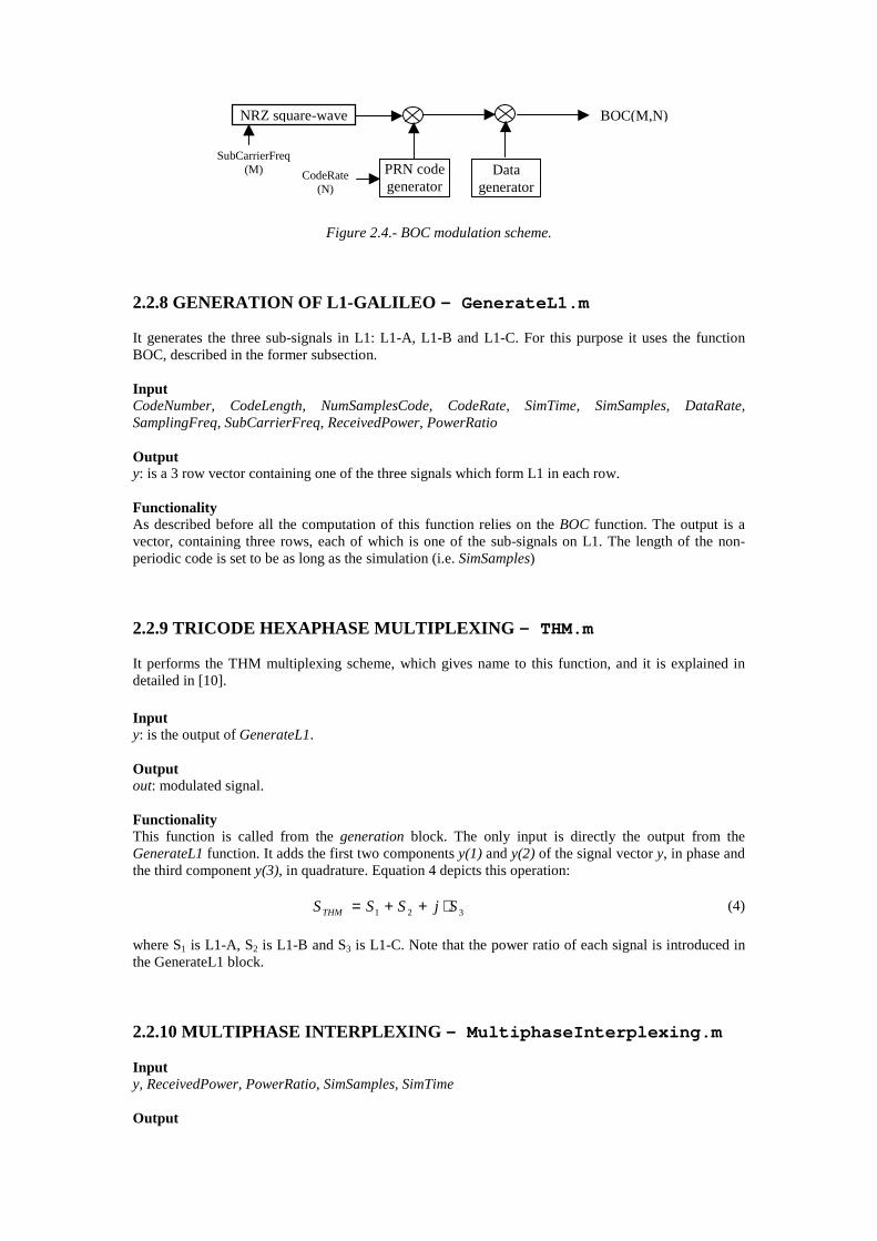
Figure 2.4.- BOC modulation scheme. 2.2.8 GENERATION OF L1-GALILEO - GenerateL1.m It generates the three sub-signals in L1: L1-A, L1-B and L1-C. For this purpose it uses the function BOC, described in the former subsection. Input CodeNumber, CodeLength, NumSamplesCode, CodeRate, SimTime, SimSamples, DataRate, SamplingFreq, SubCarrierFreq, ReceivedPower, PowerRatio Output y: is a 3 row vector containing one of the three signals which form L1 in each row. Functionality As described before all the computation of this function relies on the BOC function. The output is a vector, containing three rows, each of which is one of the sub-signals on L1. The length of the non-periodic code is set to be as long as the simulation (i.e. SimSamples) 2.2.9 TRICODE HEXAPHASE MULTIPLEXING - THM.m It performs the THM multiplexing scheme, which gives name to this function, and it is explained in detailed in [10]. Input y: is the output of GenerateL1. Output out: modulated signal. Functionality This function is called from the generation block. The only input is directly the output from the GenerateL1 function. It adds the first two components y(1) and y(2) of the signal vector y, in phase and the third component y(3), in quadrature. Equation 4 depicts this operation:

321 SjSSSTHM ⋅++= (4) where S1 is L1-A, S2 is L1-B and S3 is L1-C. Note that the power ratio of each signal is introduced in the GenerateL1 block. 2.2.10 MULTIPHASE INTERPLEXING - MultiphaseInterplexing.m Input y, ReceivedPower, PowerRatio, SimSamples, SimTime Output

NRZ square-wave

PRN code generator

Data generator

BOC(M,N)

SubCarrierFreq (M) CodeRate

(N)

out: L1 modulated signal. Functionality It carries out the implementation of the Coherent Adaptative Subcarrier Modulation (CASM) technique, studied in [3] and [11] which aims to get a constant envelope, and which herein is used as a multiplexing rather than a modulating scheme. From the three different options given in [5], option 2 was chosen5. This leads us to the following equation:

( ) ( )[ ])()()()(2)(2)(233

2)( tetetetejtetePtS CBAACB +⋅−−= (4)

where eA, eB and eC account for L1-A, L1-B and L1-C respectively. Notice that in the function the values of y are divided by the PowerRatio since the CASM already takes this into account, thus forcing us to work with the “power unbalanced” sub-signals. 2.2.11 ALTERNATIVE BOC - AlternativeBOC.m Input CodeLength, CodeRate, DataRate, SubCarrierFreq, SamplingFreq, NumSamplesCode, SimTime, ReceivePower, SimSamples, CodeNumber Output Out: vector containing the modulated signal. Functionality The alternative BOC modulation, modulates the four signal contained in E5a and E5b into a single carrier. Thus the first thing this functions does, is to generate the 4 independent PRN codes corresponding to E5a-I, E5a-Q, E5b-I and E5b-Q; and the data bits modulated in the in-phase channels (data1 and data3). This way, the ei(t) ∈i {1,..,4} signals are created, where the codes are e1=E5b-I, e2=E5a-I, e3=E5b-Q and e4=E5a-Q. Finally it computes the sub-signals used to perform the modulation, and the output signal, which is a composition of the former sub-signals, as specified in [5]. 2.2.12 DATA GENERATION - GenData.m Input SimTime, DataRate, SimSamples Output data Functionality It generates a random data signal at DataRate bits/second. However, if DataRate equals 10.23·106, it generates a PRN sequence corresponding to the P(Y)-code. It was decided to generate the P(Y)-code like that in order to save computational load. The function generates always at least the samples corresponding to 1 bit, even if the simulation lasts less. In that case, the signal vector will be truncated to match SimSamples. 2.2.13 DOPPLER COMPUTATION - ComputeDoppler.m Input

5 The base-band equation given by [5] is somewhat erroneous since some constants are missing. See Annex A

satellite, SignalType, SamplingFreq, SimTime, data_output, PlotDoppler Output InterpDoppler: this is the interpolated doppler with an interpolation each 0.1 ms (default). Doppler_out: is the re-sampled version (to 1/SamplingFreq) of the InterpDoppler. Functionality Reads from the file data_output.txt the doppler values for the chosen satellite. These values are given each 60 seconds, thus if we want to know the doppler we have to add to each sample, an interpolation has to be carried out. The data structure of the file data_output.txt is given in Table 2.1.

Column Data 1 Time (seconds) 2 Type of satellite 3 Satellite number 4 Pseudorange (m) 5 Received Power (dBm) 6 Doppler (Hz) 7 Satellite elevation (rad)

Table 2.1.- Data format of file data_output.txt

The function searches for the given satellite number within the file and stores the doppler values in the variable doppler. The vector InterpDoppler contains the interpolated version of the values given in doppler, using the time vector timeInterp (this gives an interpolation of 1 doppler sample each 0.1 ms.- of course this value was chosen in an arbitrary way, and can be altered if necessary). Thus, the vector Doppler_out is a re-sampled version (at a rate of 1/SamplingFreq) of InterpDoppler. To do so, all the samples of Doppler_out in the interval [10-4(step-1), 10-4step[ where step ∈ N contain the same doppler value. Finally it plots the doppler profile of the selected satellite for SimTime seconds (if this was selected in parameters.m). To learn more about the interp1 function type «help interp1» in MATLAB or read the annex at the end of ComputeDoppler.m. 2.2.14 PLOTS - PlotResult.m Input y, yfilter, ychannel, PlotSpectrum, PlotTime, PlotSignalConstellation, SamplingFreq, SimSamples, ReceivedPower, PowerRatio, FilterSignal, SubCarrierFreq, CodeLength, CodeRate, NumSamplesCode, AddMP, AddNoise, SignalType, MultiplexSqueme Output There are no output variables. The output are the desired plots. Functionality Depending on the set up of the parameters function, it can plot the Spectrum, Time and Signal Constellation of the generated signal. If L1-C with no multiplexing is selected, it will present the results individually for each sub-signal. Note: the doppler profile is not plotted through this function but directly in ComputeDoppler.

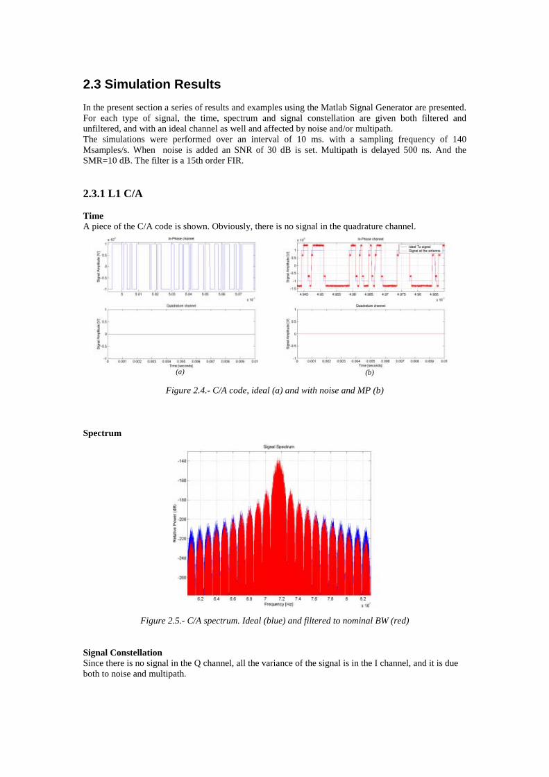
2.3 Simulation Results In the present section a series of results and examples using the Matlab Signal Generator are presented. For each type of signal, the time, spectrum and signal constellation are given both filtered and unfiltered, and with an ideal channel as well and affected by noise and/or multipath. The simulations were performed over an interval of 10 ms. with a sampling frequency of 140 Msamples/s. When noise is added an SNR of 30 dB is set. Multipath is delayed 500 ns. And the SMR=10 dB. The filter is a 15th order FIR. 2.3.1 L1 C/A Time A piece of the C/A code is shown. Obviously, there is no signal in the quadrature channel.

Figure 2.4.- C/A code, ideal (a) and with noise and MP (b) Spectrum

Figure 2.5.- C/A spectrum. Ideal (blue) and filtered to nominal BW (red)

Signal Constellation Since there is no signal in the Q channel, all the variance of the signal is in the I channel, and it is due both to noise and multipath.

(b)(a)

Figure 2.6.- C/A signal constellation, ideal (a) and with noise and MP (b) 2.3.2 L1 C/A + P(Y) Time The higher chipping rate of the P(Y)-code can be observed now on the quadrature channel.

Figure 2.7.- C/A plus P(Y) codes, ideal (a) and with noise and MP (b). Spectrum Now the first lobe of the P(Y)-code shows up, on top of which the C/A code appears.

Figure 2.8.- C/A plus P(Y) spectrum. Ideal (blue) and filtered to nominal BW (red)

(a) (b)

(a) (b)

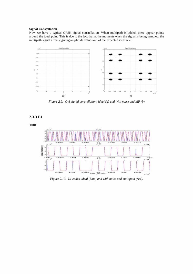
Signal Constellation Now we have a typical QPSK signal constellation. When multipath is added, there appear points around the ideal point. This is due to the fact that at the moments when the signal is being sampled, the multipath signal affects, giving amplitude values out of the expected ideal one.

Figure 2.9.- C/A signal constellation, ideal (a) and with noise and MP (b) 2.3.3 E1 Time

Figure 2.10.- L1 codes, ideal (blue) and with noise and multipath (red).

(a) (b)

Spectrum

Figure 2.11.- L1 components spectrum, ideal (blue) and filtered (red).

2.3.4 Tricode Hexaphase Modulation Time

Figure 2.12.- THM composed signal, ideal (a) and with noise and multipath (b).

(a) (b)

Spectrum

Figure 2.13.- THM spectrum, ideal (blue) and filtered (red).

Signal Constellation

Figure 2.14.- THM signal constellation, ideal (a) and with noise and multipath (b). 2.3.5 Multiphase Interplexing Time

Figure 2.15.- MI signal, ideal (a) and with noise and multipath (b).

(a) (b)

(a) (b)

Spectrum

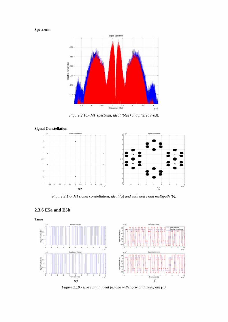
Figure 2.16.- MI spectrum, ideal (blue) and filtered (red).

Signal Constellation

Figure 2.17.- MI signal constellation, ideal (a) and with noise and multipath (b). 2.3.6 E5a and E5b Time

Figure 2.18.- E5a signal, ideal (a) and with noise and multipath (b).

(a) (b)

(a) (b)

Spectrum

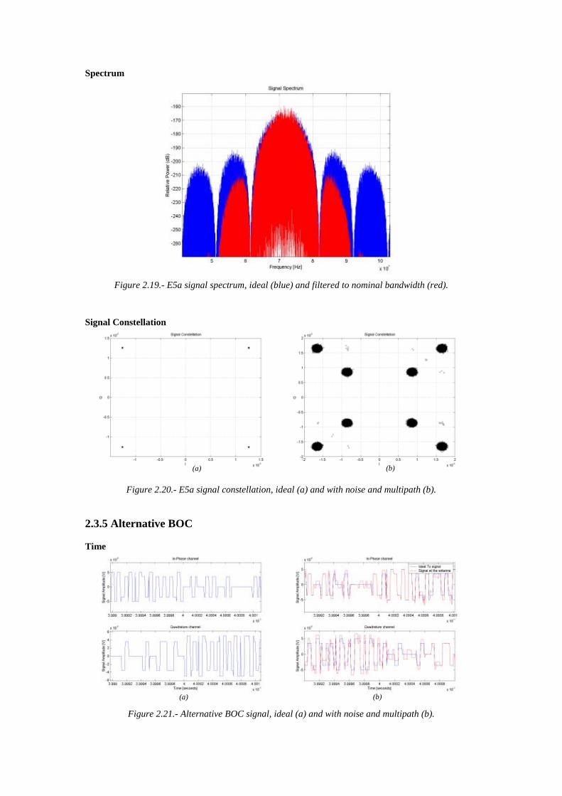
Figure 2.19.- E5a signal spectrum, ideal (blue) and filtered to nominal bandwidth (red).

Signal Constellation

Figure 2.20.- E5a signal constellation, ideal (a) and with noise and multipath (b). 2.3.5 Alternative BOC Time

Figure 2.21.- Alternative BOC signal, ideal (a) and with noise and multipath (b).

(a) (b)

(a) (b)

Spectrum

Figure 2.22.- Alternative BOC spectrum, ideal (blue) and filtered to nominal BW (red).

Signal Constellation

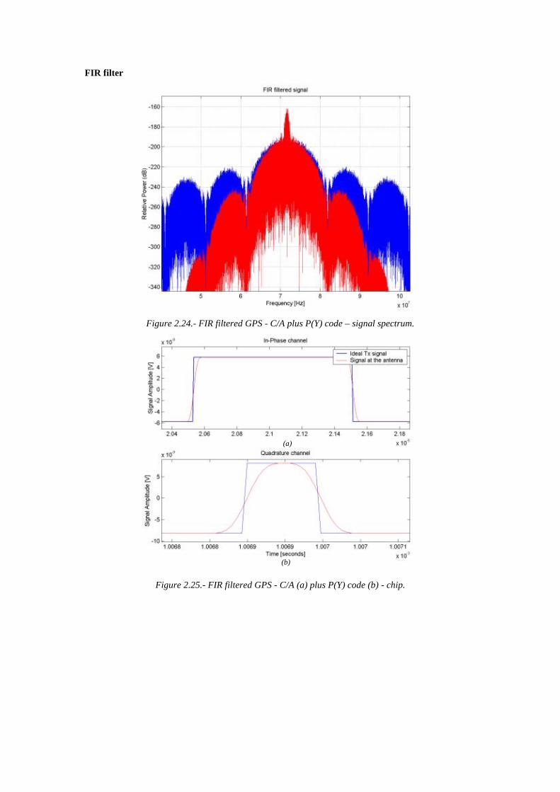
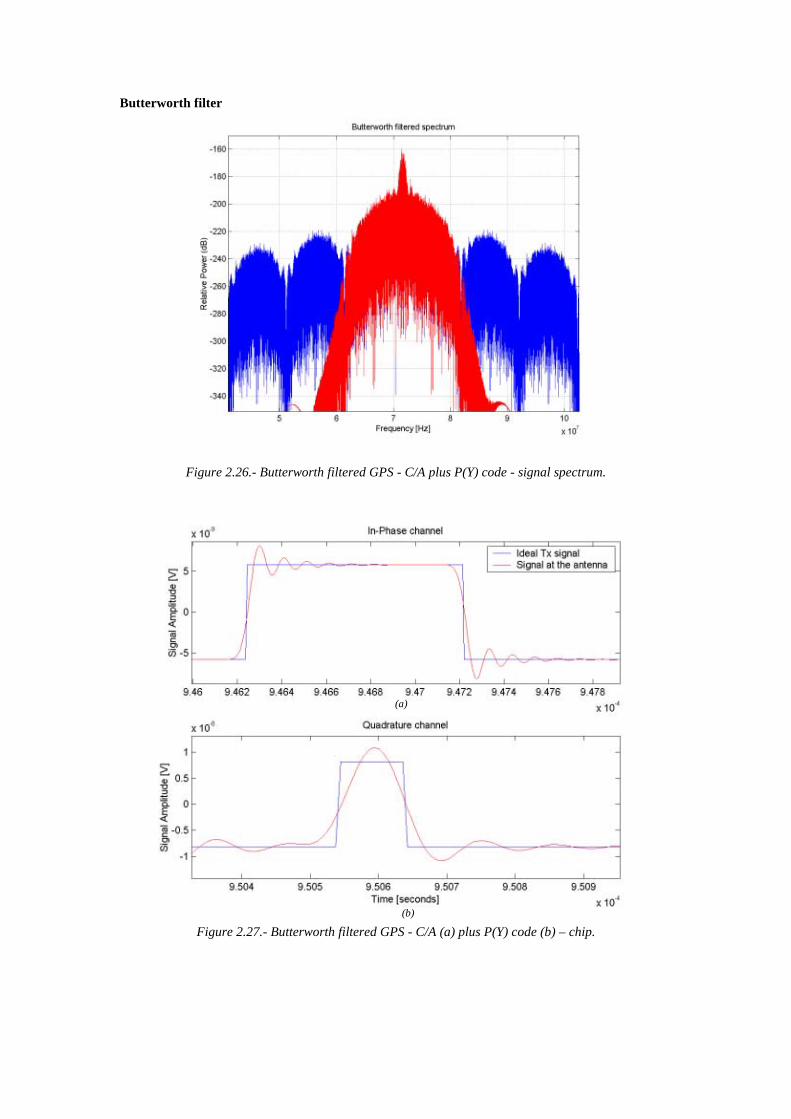
Figure 2.23.- Alternative BOC signal constellation, ideal (a) and with noise and multipath (b). 2.3.5 Filtering effect The following figures show the filtering effect due to the use of the three different filters available (FIR, Butterworth and Chebyschev). For each filter, the power spectral density and the effect of filtering one chip is shown. For all figures a GPS with C/A and P(Y) codes was generated. The user can carry out the same kind of simulations for the other more complex types of signals by means of changing the type of generated signal. Since the sampling frequency was 140x1.023 MHz, the spectrum appears centred at 70x1.023 MHz. Also note that for the same filter order, the Chebyschev filter achieve a faster falling to the stop band, accomplishing a larger stop band attenuation. As a drawback, the chips of the transmitted code (the time-domain signal) are filtered its high component frequencies, thus resulting more distorted.

(a) (b)

FIR filter

Figure 2.24.- FIR filtered GPS - C/A plus P(Y) code – signal spectrum.

Figure 2.25.- FIR filtered GPS - C/A (a) plus P(Y) code (b) - chip.

(a)

(b)

Butterworth filter

Figure 2.26.- Butterworth filtered GPS - C/A plus P(Y) code - signal spectrum.

Figure 2.27.- Butterworth filtered GPS - C/A (a) plus P(Y) code (b) – chip.

(a)

(b)

Chebyschev filter

Figure 2.28.- Chebyschev filtered GPS - C/A plus P(Y) code - signal spectrum.

Figure 2.29.- FIR filtered GPS - C/A (a) plus P(Y) code (b) - chip.

(a)

(b)

Chapter 3

VHDL HARDWARE SIGNAL GENERATOR 3.1 System Architecture The criteria to create the VHDL Signal Generator was to start with the basic blocks (which does not mean more simple). These were mainly the clock.vhd (which helped to have a clocking signal during the design) and the blocks which generate the basic ML sequences (PRNgenerator13.vhd and PRNgenerator14.vhd). The complex blocks are built using 2 or more basic or other non-basic blocks. The main file in our model is the SignalGenerator.vhd.

Besides, since thcoming out of theDAC has a 12 birepresent the dynresolution of the x9 bits. This leaves

This way, our DA

SignalGenerator

b L1-A B L1-C THM MI

CLK Enable

E5

E5a

e goal was t FPGA, a c

ts resolutionamic range , we need to 1 bit for the

C will be abl

AlternativeBOC

Figure 3.1.- High level VHDL

o program an FPGA and be abodification scheme had to be im, and on the other hand we veriof our signals (this gives a dyn set the number of bits assign to t sign. Figure 3.2 shows the latter

Figure 3.2.- 12 bit codin

e to represent values ranging fro

1 01 1001101signn

integer decimal

L1-

model.

le to see the GALILEO analog signal plemented. On one hand, the available fy that with 2 bits, we have enough to amic range of [0, 2.x]). To know the

he decimal part, which was chosen to be .

g.

m -2.998 to 2.998.

01

3.2 Building Blocks 3.2.1 alternativeboc.vhd Functionality This block groups all the blocks used to compute the Alternative BOC modulation. It uses the E5a_I, E5a_Q, E5b_I and E5b_Q, plus two DataMain blocks (which generate the data modulated on the in-phase channels). Besides it includes 4 BOC sub-blocks which generate the four BOC signals (same frequency, but with different phase, ∆Φ=π/4). The ComputeSubSignals block generates the sub-signals. Finally all the signals generated by the former blocks are converted to the 12 bits format, and then grouped in the CEA_BOC. This blocks computes the Alternative BOC modulation from the signals provided by the former blocks. Ports IN: clk: external clock signal. G_enable: general enable. OUT: E5_InPhase: the in-phase part of the Alternative BOC modulation. E5_Quadrature: the quadrature part of the Alternative BOC modulation. 3.2.2 boc.vhd and boc_l.vhd Functionality These two block generate a BOC signal but with a slight different. Since the BOC.vhd is used to generate an Alternative BOC signal, four of these blocks will be connected in cascade, in way that the first block activates the second after T/8, the second the third after the same time, and so on, until the fourth is active. Like this, four BOC signals are generated with an offset of T/8 between two consecutive blocks. The signal control is used to generate the T/8 shift. Once the shift is generated, control will be ‘0’, and the permanent regime where the BOC signal is generated will be set.

Figure 3.3.- Interconnection of four BOC.vhd. On the other hand, BOC_L.vhd is used to generate a normal BOC signal for the L1 signal. Note that half clock periods are used for the counter on BOC.vhd, while full clock periods are used in the BOC_L.vhd. This is due to the fact that more precision is needed in BOC.vhd, since one has to be able to count the exact number of clock cycles to generate precisely a shift of T/8. It was founded that by counting half cycles, the former shift was achieved (while by choosing full cycles, the obtained shift was not exactly T/8). Further investigation is encouraged in this issue to find out other possible ways to do that. Ports

enable_in BOC

wait T/8 enable_out

enable_in BOC

wait T/8 enable_out

enable_inBOC

wait T/8 enable_out

enable_in BOC

wait T/8 enable_out

‘1’

dumb

BOC (t) BOC (t-T/8) BOC (t-T/4) BOC (t-3T/8)

IN: BOC_freq: it is the frequency of the BOC signal. clk: external clock signal. G_enable: general enable. enable_in: enable block. OUT: enable_out: this signal is used to enable the following BOC block. BOC_period: it marks the boundaries of a BOC pulse. Used for synchronization purposes. BOC_out: is the generated BOC signal. 3.2.3 cea_boc.vhd Functionality It generates de Alternative BOC modulation from the sub-signals given by the ComputeSubSignals block, the PRN codes and the data signals. To compute the additions and subtractions, first we find out which will be the resulting sign of the XOR operation. If it is positive, we add that result to the accumulated value, if negative, we subtract it. Let us see an example: AlternativeBOC_Id<=(AlternativeBOC_Ic + Sc134_I) when (E5b_I_12b(11) xor data1_12b(11)

xor E5b_Q_12b(11) xor E5a_Q_12b(11)) = '0' else

(AlternativeBOC_Ic - Sc134_I); In the former piece of code, the sign of the different components of the product is checked. This is done by looking in the MSB (11th) of the 12 bit word containing the coded value of the represented signal. When the overall product is positive (the MSB bit will be zero) then the sub-signal Sc134_I is added, else, it is subtracted. Ports IN: E5a_I_12b, E5a_Q_12b, E5b_I_12b, E5b_Q_12b: 12 bit coded PRN codes. data1_12b, data2_12b: data signal. Sc1_I, Sc2_I, Sc3_I, Sc4_I, Sc123_I, Sc124_I, Sc134_I, Sc234_I, Sc1_Q, Sc2_Q, Sc3_Q, Sc123_Q, Sc124_Q, Sc134_Q, Sc234_Q: clk: external clock signal. OUT: AlternativeBOC_out_I: 12 bit coded in-phase component of the generated Alternative BOC. AlternativeBOC_out_Q: 12 bit coded quadrature component of the generated Alternative BOC. 3.2.4 clock.vhd Functionality It generates a clock signal. Since it is an external signal, its period will be also defined from the outside. However in this model, like stated before, an external frequency of 160x1.023 MHz is assumed in order to set the internal counters. This block is only designed for serving as a test bench input. In the final model the clock will be an external signal coming in the FPGA. Ports OUT: clk: clocking square signal. In the final model, it is an external signal fed to the FPGA.

3.2.5 compute_mi.vhd Functionality Computes the Multiphase Interplexing scheme used to multiplex the three signal components (A,B and C) of L1. The technique used to implement this multiplexing scheme was to compute off-line all the possible results depending on the values of the incoming signals L1-A, L1-B and L1-C. Since we have a little number of different signals (only three) this is faceable. Doing so, 8 different constants are obtained. Then a kind of true table is build up, where a result is assigned for each combination of the signals. InPhase <= c00304 when L1_A_12b=m_one and L1_B_12b=m_one and L1_C_12b=m_one else cm0303 when L1_A_12b=m_one and L1_B_12b=m_one and L1_C_12b=one else

···

···

c00304, cm0303, m_one and one are pre-calculated constants (stored as a 12 bit standard logic vector). Ports IN: L1_A_12b: 12 bit coded L1-A signal. L1_B_12b: 12 bit coded L1-B signal. L1_C_12b: 12 bit coded L1-C signal. OUT: InPhase: in-phase component of the generated multiplexed signal. Quadrat: quadrature component of the generated multiplexed signal. 3.2.6 computesubsignals.vhd Functionality Computes the sub-signals necessary to create the Alternative BOC modulation. Note that this block does not have a general enable signal since it is a combinational one. This means that the value of its output ports only will change when any of the input signal changes. Since some of the input signals come from sequential blocks (the BOC signals), if that block is not enable neither will be this, and all signals will remain with their initial value. Like in the former block all the possible values for the generated sub-signals are computed a priori and stored. Then the same sort of combinational true table is build up for each sub-signal. Ports IN: BOC_sinmPi4, BOC_sin, BOC_sinPi4, BOC_cos: BOC signals shifted Π/4 between each consecutive signal clk: external clock signal. OUT: Sc1_I, Sc2_I, Sc3_I, Sc4_I, Sc123_I, Sc124_I, Sc134_I, Sc234_I, Sc1_Q, Sc2_Q, Sc3_Q, Sc4_Q, Sc123_Q, Sc124_Q, Sc134_Q, Sc234_Q: set of generated sub-signals. 3.2.7 datagenerator2.vhd Functionality It is a simplified version of the block PRNgenerator13.vhd. Since the generated data bits are not an important issue in our model, the bits are generated as a PRN sequence. However, to avoid to start

generating bits before they can be modulated on the correspondent PRN code, the block does not start until enable=’1’. This enable will be linked to a marker signal output by a PRNmain block (making sure that the first bit will start when the first chip of the PRN code is available). Ports IN: DataRate: rate at which the data is generated. clk: clock signal connexions: like in PRNgenerator13.vhd, to set which cells feed back the LFSR (see 3.2.13) enable: if ‘1’, the block is activated. G_enable: general enable. OUT: bit_out: as it changes from 0 to 1 and vice versa, it signals when a bit transition occurs. Data: generated data bits. 3.2.8 datamain.vhd Functionality It is the data generator block. For debugging purposes, it incorporates a clock component (commented on the general simulation mode). Thus, it includes one datagenerator2 block, having the same input and output ports. The sequence vector is defined on the upper level architecture (i.e. on the immediate upper block that includes datamain as a sub-block). Ports IN: DataRate: same as on datagenerator2.vhd. clk: same as on datagenerator2.vhd. sequence: same as connexions on datagenerator2.vhd. enable: same as on datagenerator2.vhd G_enable: same as on datagenerator2.vhd OUT: bit_out: same as on datagenerator2.vhd Data: same as on datagenerator2.vhd 3.2.9 E5a.vhd Functionality It is formed by three main blocks: an E5a_I for the in-phase component, a E5a_Q for the quadrature component and a DataMain for the data modulated on the in-phase channel (the block also carries out this modulation “E5a_I_Out XOR Data”). On addition to this, there are two more blocks (corresponding to the same Std_to_12bit component, see 3.2.34) with the aim of converting to 12 bits the output values of the in-phase and quadrature channels. Ports IN: clk: external clock signal. G_enable: general enable. OUT: E5a_InPhase_12b: 12 bit coded in-phase channel. E5a_Quadrature_12b: 12 bit coded quadrature channel.

3.2.10 E5a_I.vhd Functionality It is formed by two different blocks: a E5a_I_PRNmain which provides the Gold code, and a E5a_I_TieredCode which modulates that Gold code with a Lidner code.

Figure 3.4.- High level scheme of Ea5_I.vhd

Ports IN: offsetI: is the offset to be applied on one of the two ML sequences in E5a_I_PRNmain in order to generate the desired Gold code. clk: external clock signal. G_enable: general enable. OUT: E5a_I_Out: main output of the block. It is directly the output of the E5a_I_TierdCode block. marker_aux: it signals when the Gold code starts to be generated (it will also match the time instant when the Tiered code begins). ChipOut: signals a chip transition of the generated PRN code. 3.2.11 E5a_I_PRNmain.vhd Functionality The same way as the basic block PRNmain14 (see 3.2.32), it has the function of generating a Gold code. However, unlike that former block, it includes one more input (offsetI, whose value is now set by upper level blocks) and output (ChipOut, which marks the chip boundaries). Ports IN: offsetI: is the offset to be applied on one of the two ML sequences in E5a_I_PRNmain in order to generate the desired Gold code. clk: external clock signal. G_enable: general enable. OUT: ChipOut: signals a chip transition of the generated PRN code. marker: it signals when the Gold code starts to be generated. GoldCode: generated Gold code. 3.2.12 E5a_I_TieredCode.vhd Functionality It performs the XOR of a stored Lidner code of length 20, with a Gold code. The block will start functioning when marker is set to ‘1’ (that is, when the first chip of the Gold code is available). When the last bit of the Lidner code is used, it will start again from the first bit (LidnerCode20(0)).

E5a_I_PRNmain E5a_I_TieredCodeclk

offsetI E5a_I_out Gold Code

E5a_I

The variables q_var and p_var are created as auxiliary forms of q and p. The constant limit of 10230 (for p_var) is the length of the Gold code (it should not change, since it was set this way for E5a). For q_var it is obviously 20 since it is the length of the Lidner code. Ports IN: GoldCode: Gold code. LidnerCode20: is the Lidner code of length 20. ChipOut: it signals when a new chip from the Gold code is generated marker: it signals when the Gold code starts to be generated. G_enable: general enable OUT: E5a_I_Out: the XOR of the incoming Gold code with the pre-stored Lidner code. 3.2.13 E5a_Q.vhd It is equivalent to the block E5b_I.vhd, and it can be explained the same why just changing a by b in any variable. However it lacks a marker output. This marker has the purpose of synchronizing the modulation of the data bits on the PRN code. Since no data is on the Q channel, this output is not needed here 3.2.14 E5a_Q_PRNmain.vhd It is equivalent to the block E5a.vhd, and it can be explained the same why just changing a by b and I by Q in any variable. 3.2.15 E5a_Q_TieredCode.vhd This block generates a Tired code from the combination of a Lidner code (length 100 chips) and a truncated Gold code. It is equivalent to the block E5a_I_TieredCode.vhd, and it can be explained the same why just changing a by b in any variable. 3.2.16 E5b.vhd It is equivalent to the block E5a.vhd, and it can be explained the same why just changing a by b in any variable. 3.2.17 E5b_I.vhd It is equivalent to the block E5a_I.vhd, and it can be explained the same why just changing a by b in any variable. 3.2.18 E5b_I_PRNmain.vhd It is equivalent to the block E5a_I_PRNmain.vhd, and it can be explained the same why just changing a by b in any variable.

3.2.19 E5b_I_TieredCode.vhd This block generates a Tired code from the combination of a Lidner code (length 4 chips) and a truncated Gold code. It is equivalent to the block E5a_I_TieredCode.vhd, and it can be explained the same why just changing a by b in any variable. 3.2.20 E5b_Q.vhd It is equivalent to the block E5b_I.vhd, and it can be explained the same why just changing a by b in any variable. However it lacks a marker output. This marker has the purpose of synchronizing the modulation of the data bits on the PRN code. Since no data is on the Q channel, this output is not needed here. 3.2.21 E5b_Q_PRNmain.vhd It is equivalent to the block E5a_I_PRNmain.vhd, and it can be explained the same why just changing a by b in any variable. 3.2.22 E5b_Q_TieredCode.vhd This block generates a Tired code from the combination of a Lidner code (length 100 chips) and a truncated Gold code. It is equivalent to the block E5a_I_TieredCode.vhd, and it can be explained the same why just changing a by b in any variable. 3.2.23 L1_A.vhd Functionality This block groups all necessary sub-blocks in order to generate the L1-A signal (PRNgeneratorA, DataMain and BOC_L), in the following way: L1_A_Out <= (output0 xor output1) xor BOC_out xor Data ; output0 and output1 are the ML sequences used to build up the Gold Code. In the real signal the code on L1-A is created as the concatenation of a series of Gold Codes. In our model, the same PRN code is being generated all the time. A 13 register LFSR was chosen (thus, it is generated in a very similar way as PRNgenerator13, but without having to take into account the offset between the two sequences, thus it is a simplified version of PRNgenerator13). Another possibility was to generate a Gold code of 8190 chips, store it in a std_logic_vector, and then do the XOR with an “on-the-fly” generated Gold code. This other possibility would make use of the file L1_A_TieredCode.vhd, a file almost identical to the L1_C_TieredCode.vhd. Ports IN: clk: external clock signal. G_enable: general enable. OUT: L1_A_12b: 12 bit coded L1-A signal.

3.2.24 L1_A_TieredCode.vhd Not used in the final model. 3.2.25 L1_B.vhd Functionality This block groups all necessary sub-blocks in order to generate the L1-B signal (PRNmain13, DataMain, BOC_L and std_to_12bit). The code rate, type of generated code (via the offset), and BOC frequency are defined here. Ports IN: clk: external clock signal. G_enable: general enable. OUT: L1_B_12b: 12 bit coded L1-A signal. 3.2.26 L1_C.vhd Functionality This block groups all necessary sub-blocks in order to generate the L1-C signal (L1_C_PRNmain, L1_C_TieredCode, BOC_L and std_to_12bit). The BOC frequency is defined here. The parameters concerning the Gold code are set in the L1_C_PRNmain block. Ports IN: clk: external clock signal. G_enable: general enable. OUT: L1_B_12b: 12 bit coded L1-A signal. 3.2.27 L1_C_TieredCode.vhd Functionality It generates a Tiered code from a predefined Lidner code (length 25) and a truncated Gold code. The functionality is identical to that of other TiredCode.vhd type files used in the model. Ports IN: GoldCode: 8184 chip long Gold code. LidnerCode25: Lidner code. ChipOut: not used in the final version. Marker: it marks when the Gold code is available. G_enable: general enable. Clk: external clock signal. OUT: L1_C_Out: generated Tiered code.

3.2.28 MI.vhd Functionality It generates a Multiphase Interplexed signal used to multiplex the three signals on L1 (A,B and C) onto a single carrier. The result are two 12 bit vectors containing the coded version of the complex base-band signal. It groups all the necessary blocks to do so (L1_A, L1_B, L1_C and Compute_MI). Ports IN: clk: external clock signal. G_enable: general enable. OUT: MI_InPhase: in-phase component of the generated signal. MI_Quadrat: quadrature component of the generated signal. 3.2.29 PRNgenerator13.vhd Functionality It generates a ML sequence of length CodeLength, at a CodeRate chips/s and using a 13 cell LFSR. To generate a Gold code, two PRNgenerator13 blocks are needed. They are interconnected so that one starts generating the ML sequence starting with LFSR1 initialised to {1111111111111}. The other block is not activated until Offset chips are counted by the first block. At this precise time, the second block starts to generate the ML sequence (since chipEnable >= Offset will be ‘1’), and the two sequences start to be added, chip by chip to form the Gold Code. Like this, the two blocks generate the same sequence but with Offset chips of difference. Ports IN: connexions: vector containing the cells of the LFSR which contribute to the feedback. Changing this vector will change the generated sequence. CodeRate: rate of the code to generate Offset: of one of the ML sequences with respect to the other. Changing this will generate different PRN codes. Note that the offset used follows the following rule: offset = 214-StatedOffset - 1,

1 - etStatedOffs-2 offset N=

where StatedOffset is the offset declared on [Astrium], and N is the length of the register (in this case 13). CodeLength: length of the final Gold code. clk: clock signal. type_block: indicates if the block is type=’1’ (starts generating sequence from the beginning) or type=’0’ (starts generating sequence when chip reaches Offset) G_enable: general enable. OUT: marker: output: is the generated ML sequence (is directly the output of the LFSR). 3.2.30 PRNgenerator14.vhd It generates a ML sequence using a 14 register LFSR. It is similar to PRNgenerator13, with the difference of having one more output, ChipOut. This signal marks the chip boundary, and in the

beginning it was used to synchronize the XOR addition of the Gold code with the Lidner code to form a Tiered code. 3.2.31 PRNmain13.vhd Functionality It is the block that generates a Gold code from two ML sequences offset by offset chips. The sequences will be different and depend upon the value of the connexions vector (connexion1 and connexion2). It is hence formed by two PRNgenerator13 blocks. The block simply adds (XOR) the outputs of the two blocks to produce the Gold code. It is here were one can change the values of the CodeRate, Offset (see [Astrium]), CodeLength and the feedback connexion vectors in order to generate different types of Gold Code using 13-cells long LFSR. Ports IN: clk: clock signal. G_enable: general enable. OUT: marker: it points out when the Gold code starts to be generated GoldCode: generated Gold code. 3.2.32 PRNmain14.vhd Functionality Basically it does the same as the former PRNmain13, but using two PRNgenerator14 blocks. 3.2.33 SignalGenerator.vhd Functionality This is the main file of the VHDL model. It contains the main sub-blocks that allow generating all the signals. A given signal will be generated if there is a ‘1’ in the position assign to that signal according to Table 3.1.

Signal «enable» vector E5a “00000001” E5b “00000010” Alternative BOC “00000100” L1-A “00001000” L1-B “00010000” L1-C “00100000” L1 (MI) “01000000” L1 (THM) “10000000”

Table 3.1.- Value of enable to generate each GALILEO signal.

Ports IN: enable: this 8 position vector indicates which is the signal that is going to be generated. OUT: InPhase_out: in-phase component of the generated signal.

Quadrat_out: quadrature component of the generated signal. 3.2.34 Std_to_12bit.vhd Functionality It converts a std_logic type to a 12 bit coded version. The criteria was to assign –1 to the logic level “1” and +1 to the logic level “0”. Ports IN: input: standar_logic bit. OUT: output: 12 bit coded version of the input. 3.2.35 THM.vhd Functionality The same way as the MI.vhd, it generates a signal which is the multiplex of the three signals on L1 (A,B and C). The present block, however, it performs the Tricode Hexaphase Modulation. The result are two 12 bit vectors containing the coded version of the complex base-band signal. It groups all the necessary blocks to do so (L1_A, L1_B and L1_C) The process Compute_THM, executes the operations to modulate the signals (in this case, very simple as it can be easily depicted). Ports IN: clk: external clock signal. G_enable: general enable. OUT: THM_InPhase: in-phase component of the generated signal. THM_Quadrat: quadrature component of the generated signal. 3.3 Doing Simulations Standard simulation If the purpose is to simulate one of the GALILEO signals, as a whole, that should be done from the SignalGenerator.vhd file. As shown on Table 3.1, by setting to “1” the appropriate bit of the port enable, one can generate the desired GALILEO signal. In order to see the generated signal, the wave window should be open before the simulation is started and load the appropriate signal environment. To do that, go to File Load Format, and then choose the file *.do corresponding to the selected signal. For example, if we want to simulate the E5a signal, first we will set enable to “0000001 and then load in the wave window the output signals and variables corresponding to E5a. Loading the file SG.do allows to see any possible generated signal. This is a common file for all signals when the standard type of simulation is wanted. At this point we only need to select the simulation time (something between 1 and 100 ms. would appropriated in order to see more than one code period and some data bit transitions). Then, we click on the Run button.

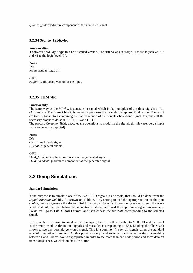
Once the simulation is completed, the in-phase and quadrature value corresponding to L1-C will be available on the wave window, highlighted in cyan. One can see that we have all GALILEO signals on the wave window. However only E5a has been generated. The other remain zero, constant or undefined for the whole simulation time. An example of such a simulation is shown in Figure 3.5. The output signals for E5a are inphase_out1 and quadrat_out1, which of course match inphase_out and quadrat_out respectively since it is being the signal generated.

Figure 3.5.- Simulation of E5a from SignalGenerator.vhd.

Block simulation Apart from the standard simulation, one may want to see what is going on inside the building blocks that form the pieces of the larger upper level block for a given signal. It is also possible to do that. However some minor manual changes have to be done and some considerations have to be taken into account. The first thing to do is to load the block of interested. Let us explain this with an example. Hence let us load the block E5a.vhd. That will allow us to check what is happening inside that block in a more accurate way. Then like in a standard simulation we open a wave window and load the file containing the signals and variables for that block. That is the E5a.do. Now let’s edit a bit the E5a.vhd file. Two things must be done: 1) Remove the clock input (clk) port from the entity. For that, simply comment the consequent line in the entity:

-- clk : in std_logic; 2) Create a clock component in the architecture. For that, simply uncomment the component declaration from the architecture,

component CLOCK port ( clk : out std_logic); end component;

uncomment also the instantiation of that component after the begin,

B0 : CLOCK

port map (clk => clk);

and create a signal, to be able to feed that clock signal to the underlying blocks; that is, uncomment also the corresponding line in the signal declaration at the architecture,

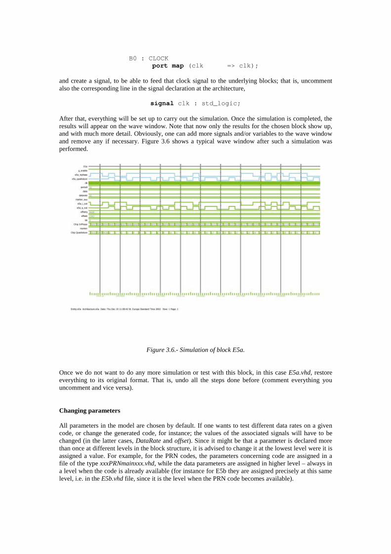
signal clk : std_logic; After that, everything will be set up to carry out the simulation. Once the simulation is completed, the results will appear on the wave window. Note that now only the results for the chosen block show up, and with much more detail. Obviously, one can add more signals and/or variables to the wave window and remove any if necessary. Figure 3.6 shows a typical wave window after such a simulation was performed.

Figure 3.6.- Simulation of block E5a.

Once we do not want to do any more simulation or test with this block, in this case E5a.vhd, restore everything to its original format. That is, undo all the steps done before (comment everything you uncomment and vice versa). Changing parameters All parameters in the model are chosen by default. If one wants to test different data rates on a given code, or change the generated code, for instance; the values of the associated signals will have to be changed (in the latter cases, DataRate and offset). Since it might be that a parameter is declared more than once at different levels in the block structure, it is advised to change it at the lowest level were it is assigned a value. For example, for the PRN codes, the parameters concerning code are assigned in a file of the type xxxPRNmainxxx.vhd, while the data parameters are assigned in higher level – always in a level when the code is already available (for instance for E5b they are assigned precisely at this same level, i.e. in the E5b.vhd file, since it is the level when the PRN code becomes available).

Chapter 4

Recommendations and Future Work In this last chapter some recommendations and some guidelines about things which need to be improved and/or introduced as new elements in the model will be given. 4.1 Matlab Model The Matlab model is completely functional, but it could be improved if one followed the next recommendations:

- Verify the (negative) delay introduced in the filtered signal in order to make it match the ideal one (for graphical representation purposes). Apart from the FIR filter, the other delays have been deducted from experience rather than from theory. This is important in order to obtain a valid signal constellation plots (and also in synchronization issues in a future Matlab Galileo Receiver).

- Even if the data modulated on the different signals is not of importance, it will be if we want to feed the signal to a receiver (since it will check the frames, sub-frames, etc in order to synchronize to the system). Thus the addition of these issues, plus a CRC (to check bit errors) becomes important only in a later stage.

- Also because of synchronization issues (but now in a physical chip level), introduce a random delay in the generated PRN code, since the code will not generally reach the receiver starting with chip #1.

- Use more complex channel models. This implies the coding of new multipath models not only consisting on a reflected ray (use the multipath models proposed by the University of Vigo).

- Introduce interference (Wide Band and Narrow Band). - In the present model, the file data_ouput.txt is only used to extract the doppler information

associated with the selected satellite. However, as seen in Section 2.13, the file contains some more useful data. For instance, the pseudorange could be used to adjust the received power depending on the satellite’s distance to the receiver; the elevation could be use in conjunction with the multipath model so that more multipath would be added for low elevation satellites.

- Introduce pulse compression/expansion due to doppler. Indeed, since the dynamics of the pair satellite-user introduce doppler, this means the carrier frequency will be increased or reduced around the nominal value as seen in Figure 4.1.

- Add the possibility of generating more than one type of signal (channel) at a time. Also the possibility of generating mixed GALILEO-GPS scenarios. This could be done “on-the-fly”, meaning that the different signals would be generated in parallel, or off-line, that is, the signals would be generated sequentially, saved in a file or matlab variable, and added a posteriori.

- Finally create a GUI to ease the interaction of the user with the model.

Figure 4.1.- Pulse compression due to different carrier frequency because of Doppler effect.

4.2 VHDL Model The VHDL model was completed almost in its totality. The debugging of the code was started using Synplify Pro 7.1 and although all errors were corrected, there still remained several warnings. Most of these warnings are due an inferred latch due to a missing signal assignment and/or to the lack of signal in the sensitivity list of some functions. Hence the first thing one should try to achieve is to get rid of these warnings.

- Once the code is completely synthesizeable (there are no warnings left), the last step will be left, which consists on programming an FPGA mounted on an evaluation board.

- After that the output signals should be verified in the lab and check that the output match the expected type of signal. For that the use of a digital oscilloscope and a spectrum analyser might be needed.

- After solving all possible problems, the model can be enhanced adding a series of new elements in order to obtain a more complete and realistic signal.

- This elements should include a noise and a multipath generator. For the former, a PRN generator set to generate a code with a rate higher than that of the signal (for instance 10 times higher) could be used. See Figure 4.2. The addition of multipath is less tricky since it only implies to duplicate the generated signal, scale it and delay it. The addition of noise and/or a multipath signal implies that the 12 bit coding might have to be revised since the dynamic range will be now somewhat higher.

Figure 4.2.- Addition of digital white noise.

- Addition of several signals at the same time. This, as in the case of adding multipath implies a

redefinition of the distribution of the 12 bits used to convert the signal from digital to analog (there will be needed at least 1 bit more to represent the integer part of the number).

ANNEX A

Computation of CASM Let us have three signals which, according to notation used in [5] are modulated in a single carrier as specified in Equation A.1:

)mtsin()t(eP2)mtcos()t(eP2)t(s so22so11 ΦωΦω +⋅−+⋅= (A.1) where Φs(t) is a function of e1, e2 and e3. Also, since Φs belongs to {-1,+1}, then,

)msin(s)smsin(

)mcos()smcos(

ΦΦ

Φ

=

=

thus, we can rewrite A.1 like:

[ ][ ] )tosin()msin()t(s)t(1e2P2)mcos()t(2e2P2

)tocos()msin()t(s)t(2e2P2)mcos()t(1e1P2

)tosin(Qs)tocos()t(Is)t(s

ωΦ

ωΦ

ωω

⋅+⋅

−⋅−⋅

=−=

(A.2)

This can be seen as the combination of 4 signals:

[ ] [ ] )tosin()t(4u)t(3u)tocos()t(2u)t(1u)t(s ωω +−−= (A.3) Φs(t) is taken to be,

)t(e)t(e)t( 32s ⋅=Φ Then making the following assignments e1 = SB (L1-B), e2 = SA (L1-A) and e3 = SC (L1-C), which corresponds to option 2 (see Table 2.6 in [5]) and taking into account the power distribution of the L1 signals, it turns that PA=P/2, PB=PC=PA/2. Then separating the in-phase and quadrature components and substituting, we obtain:

[ ])t(e)t(e33P22

31)t(e2

32)t(e2P2

31

31)t(e)t(e)t(eP

942

32)t(eP

922)t(s

CBCB

CAABI

−=

⋅−

=⋅−⋅= (A.4a)

[ ])t(e)t(e)t(e)t(e233P2

32)t(e)t(e)t(e)t(e

322

3P2

31)t(e)t(e)t(eP

922

32)t(eP

942)t(s

CBAACBAA

CABAQ

−⋅=

−

=⋅−⋅= (A.4b)

So, grouping the two components we obtain the final transmitted signal:

( ) ( )[ ])t(e)t(e)t(e)t(e2j)t(e)t(e33P22)t(s CBAACB −⋅−−= (A.5)

References [1] Proakis, Communication Systems Engineering, Ed. Prentice Hall. [2] Astrium, “Spreading Code Design”, Doc.No. GAL2-ASMD-TN-42154-003, 27 May 2002. [3] P.A. Dafesh, T.M. Nguyen, S. Lazar, “Coherent Adaptative Subcarrier Modulation (CASM) For GPS Modernization”, ION GPS 99. [4] John W. Betz, “The Offset Carrier Modulation For GPS Modernization”, ION GPS 99. [5] Astrium, “Navigation Signal-in-Space Definition: End-to-End Performance Test Plan”, Issue 1, Rev.1, Doc.No. GAL2-ASMD-RP-42156-003, 28 May 2002. [6] European Commission Signal Task Force, “Technical Annex to GALILEO SRD Signal Plans”, Issue 1, Ref-STF-annexSRD-2001/003, 18 Jul 2001. [7] “Changelog on ESA-APPNS-REQ-000111”, Issue 4, ESA-APPNG-ICD-00103-SED, 16 Jan 2002. [8] “Satellite Signal in Space Interface Requirements”, Issue 2, Rev. 1, Ref. ESA-APPNS-REQ-000111, pages 137-159, 1 Aug 2002. [9] “System Requirements Document”, Issue 1, Rev. 1, Corr. 1, Ref. ESA-APPNS-REQ-000111, 24 Jul 2001. [10] S.H. Raghavan, J.K. Holmes, S. Lazar, M. Bottjer, “Tricode Hexaphase Modulation for GPS”, The Aerospace Corporation (white paper). [11] P.A. Dafesh, L.Cooper, M. Partridge, “Compatibility of the Interplex Modulation Method with C/A and P(Y) code Signals”, ION GPS 2000.