Harvard Institute forInternational Development

HARVARD UNIVERSITY

Development Discussion Papers

Empirical Investigation of One OPEC Country’sSuccessful Non-Oil Export Performance

Yana van der Meulen Rogers

Development Discussion Paper No. 474November 1993

© Copyright 1993 Yana van der Meulen Rogersand President and Fellows of Harvard College

HIID Development Discussion Paper no. 474

Empirical Investigation of One OPEC Country's Successful Non-Oil Export Performance

Yana van der Meulen Rodgers*

Abstract

This study evaluates the contribution of exchange rate devaluation and economicreform to Indonesia's rapid non-oil export growth from 1975 to 1990. The studyestimates structural supply and reduced form equations for Indonesia's six largest non-oil exports. I show the importance of disaggregating the data, having a more flexiblefunctional form, and separating policy variables to obtain a richer description ofexchange rate and other policy effects on trade than previous studies. Results indicatethat although agricultural exports experience bad luck from foreign shocks, policyinduced price signals and improved investment incentives work successfully to diversifyand promote Indonesia's trade. F14 Country and Industry Studies of Trade; O19International Linkages to Development.

Yana van der Meulen Rodgers is Assistant Professor at the College of William andMary. She worked as a Project Assistant for HIID in Jakarta from 1989 to 1990.

*I am indebted to Susan Collins, Jeffrey Lewis, Henry Rosovsky, Michael Roemer, and Bill Rodgers fortheir useful suggestions and their support. I also thank Richard Cooper, John Leahy, Michael McCarthy,Jonathan Morduch, Peter Timmer, Tom Tomich, and members of the Harvard University EconomicDevelopment and International Economics Seminars. Correspondence to: Yana van der Meulen Rodgers,Department of Economics, The College of William and Mary, Williamsburg, VA 23187, USA. Tel 804-221-2376; Fax 804-221-2390; EMail YVRODG@MAIL.WM.EDU.

The World Bank (1992, pp. 220-221).1

1

HIID Development Discussion Paper no. 474

Empirical Investigation of One OPEC Country's Successful Non-Oil Export Performance

Yana van der Meulen Rodgers

1. Introduction

Unlike other OPEC members and large debtor nations, Indonesia successfully

prevented stagnation in the agricultural and manufacturing sectors during and after the

1970s oil boom, and it maintained punctual repayments of large foreign debt obligations

in the 1980s when oil earnings collapsed. Rapid expansion of Indonesia's non-oil

exports contributed to an average real GDP growth rate of 5.5 percent annually during

the 1980s, compared to 0.5 percent for the Middle East and North African countries and

1.7 percent for severely indebted countries.

Non-oil export growth constitutes the highlight of Indonesia's recent trade experience;1

real average manufactured export growth of at least 28 percent annually during the

1980s rivalled Indonesia's regional neighbors.

Indonesia's non-oil export growth has helped the country to lessen its

dependence on a non-renewable natural resource as the main source of foreign

exchange. The country ranks among the world's highest debtors and requires stable

foreign exchange inflows from non-oil exports to maintain its perfect debt repayment

record. Non-oil export earnings also allow Indonesia to import more capital goods for

investment, intermediate inputs for manufacturing and agriculture, and a greater variety

of consumer goods. With the world's fourth largest population and almost 60 percent of

Pitt (1981, p. 182).2

2

the population under the age of 25, a prospering labor-intensive manufacturing sector

offers new employment opportunities. More generally, Indonesia's experience provides

major policy lessons for the numerous developing countries that still depend heavily on

a few natural resource exports.

Indonesia's trade experience raises a number of interesting questions. What

caused the rapid growth of non-oil exports in the 1980s, and in particular, what role did

government policy play? Did Indonesia survive the oil shocks and higher debt service

costs due to good planning or good luck? In 1978, Indonesia's government began to

use active exchange rate management to improve the competitiveness of non-oil

exports. Starting in 1983 the government overhauled its trade, industrial, and financial

sector policies to provide incentives for non-oil exporters and to raise domestic savings.

However, the government has also tightened restrictions in several export sectors. For

example, beginning in 1980 it progressively banned log exports to promote domestic

value added in downstream industries. Policy reform contributed to Indonesia's

transformation from a primary commodity exporter with an inward-oriented industrial

policy to a potential Asian NIC. Pitt (1981) wrote on Indonesia: "Hopes of increased

exports of manufactures, however, have not materialized. ... Thus the seeds for a more

inward-oriented manufacturing development strategy exist." Indonesia's policy reform2

helped prevent those seeds from developing.

The study estimates structural supply and reduced form equations to determine

the extent to which prices, income, and sector-specific variables can explain the

performance of Indonesia's six largest non-oil export sectors, as measured by export

Developing country sectoral export studies include Lucas (1988), Marquez and3

McNeilly (1988), Riedel (1988), and Kellman and Chow (1989).

3

shares: textiles, garments, plywood, sawnwood, coffee, and rubber. Policy changes

and world shocks affected Indonesian trade largely through prices and income. The

study focuses on the effectiveness of exchange rate devaluation, which increases the

export price in rupiah terms relative to domestic prices, in raising each sector's exports.

Imperfect substitutes, trade policy distortions, and the inclusion of nontradeables in the

domestic price series help explain why the law of one price does not hold for any

sectors over extended periods.

Empirical work for the 1975 to 1990 period provides three lessons. First,

improved price incentives, through exchange rate devaluation and inflation controls,

promote exports in sectors where Indonesia competes on the world market. Textiles,

among the fastest growing non-oil export sectors, respond more than proportionately to

the relative export price; garment, sawnwood, and coffee exports respond positively but

less than proportionately to price incentives. Second, increased domestic and

multinational investment following improvements in the investment climate makes a

significant contribution to Indonesia's manufactured export growth. Finally, while

agricultural exports experience more bad luck from foreign shocks, manufactured

exports prosper in response to the government's trade policy changes. Extensive

policy reform after 1983 has a dramatic impact on garment exports, and the log export

ban explains Indonesia's tremendous growth in plywood exports.

This study constitutes one of few empirical studies on developing country exports

at the sectoral level, and the first to estimate sectoral trade elasticities for Indonesia. 3

4

Moran (1988) estimates manufactured export elasticities for a pooled developing

country sample which includes Indonesia, and Arize (1990) estimates Indonesia's

aggregate trade elasticities. Neither the pooled nor aggregate results provide

knowledge of policy outcomes across Indonesia's major trade sectors. I also compare

the restrictive partial adjustment model used in Moran and Arize with the more flexible

Almon lag model commonly found in developed country applications, and I find a gain

in precision with the more flexible model. Finally, this study separates devaluation's

effect on relative price incentives from sector-specific policies and world shocks. This

study's methods provide a richer and more precise description of exchange rate and

other policy effects on trade.

The paper has the following organization. The next section provides an overview

of Indonesia's policy changes from 1970 to 1990. Section 3 describes the data and

trends for the six largest non-oil export sectors. Section 4 reviews the empirical

literature on developing country exports and presents the model. Section 5 reports

estimation results, and the final section summarizes.

2. Policy Reforms

Indonesian economic performance indicators in Table 1 point to strong overall

performance in the 1970s, a marked economic decline in the early 1980s, and recovery

after 1986. Fluctuations in Indonesia's economy followed oil market shocks, and the

country's real GDP growth in the early to mid-1980s dropped considerably behind other

Asian countries. Table 2 groups Indonesian policy changes from January 1970 to

December 1990, a period of gradual policy reform following a forced stabilization

program under the IMF in the late 1960s, into three corresponding sub-periods. In the

Non-oil exporters, however, had to pay a 10 percent exchange tax on the sale of4

foreign exchange earnings. In 1974 the Central Bank replaced the exchange tax with anexport tax which stayed in place until 1979. Non-oil exporters also had to sell their foreignexchange earnings to the Central Bank until 1982.

5

Micro Restriction phase from 1970 to 1981, the government increased import as well

as investment restrictions and only took limited steps to promote non-oil exports.

During the Mixed Signal period from 1982 to 1985, the government took some initial

steps to reform taxes, deregulate the financial sector, and promote non-oil exports, but

it continued to tighten import and investment restrictions. In the Steady Reform phase

from 1986 to 1990, the government passed a series of policy reforms to deregulate the

trade, investment, and financial sectors.

Continuity of sound macroeconomic policies but increasing reliance on oil

revenues and restrictive policies to promote industrialization characterized the Micro

Restriction period. Compared to most other developing countries at the time, the

Indonesian government took a bold step early in 1971 by permitting free capital

convertibility. The government made all capital transactions, including profit and

dividend remittances, freely convertible. Along with instituting free convertibility, the4

government unified, devalued, and fixed the exchange rate. The open capital system

and fixed exchange rate encouraged firms and banks to make transactions abroad,

which limited the potency of monetary policy instruments. In addition, dollar oil earnings

boomed following the 1973 oil price hike; converted into rupiah at the fixed exchange

rate and controlled by ineffective monetary policy, the oil boom led to an average

annual inflation rate of 22 percent between 1973 and 1978. In 1978, to reverse the

harmful effects of real exchange rate appreciation on non-oil exports, the government in

For studies on Dutch disease and Indonesia's policy response, see Roemer (1985),5

Glassburner (1988), and Woo and Nasution (1989).

6

a largely unexpected move devalued the rupiah by almost 50 percent. It changed the5

exchange rate regime to a managed float with infrequent large devaluations and

pegged the rupiah to a basket of trade partner currencies.

The government also offered subsidized interest rates and tax rebates to non-oil

exporters, especially in textiles and garments, and it invested heavily in agriculture.

However, the long run effects of these promotional schemes remained quite limited as

increased trade and industrial policy regulation caused large price distortions. Nor did

the government support the nominal devaluation with monetary policy; increased

inflation following the second oil boom in 1979 caused the real value of the exchange

rate to appreciate again.

During the Mixed Signal period in an effort to counteract declining oil revenues,

the Indonesian government took some initial steps to reform taxes, deregulate the

financial sector, and promote non-oil exports, but it increased the number of non-tariff

barriers and placed further restrictions on investment. Also, the government phased

out tropical log exports to encourage domestic value added in plywood and furniture. It

structured the ban by progressively raising export taxes on logs and allocating export

quotas only to those logging concessions which also had wood processing

infrastructure; after 1985 the government completely banned Indonesia's log exports.

In 1983, the government announced a second major devaluation of 39 percent to

help make Indonesian exports more competitive on the world market and encourage

domestic production of tradeable goods. In response to lower fiscal revenues from oil,

Thorbecke (1991, p.21).6

For further discussion see GATT (1991) and Barichello and Flatters (1991).7

7

the government cut expenditures on large capital intensive projects, so that between

1982 and 1986 the ratio of actual to planned capital expenditures fell from 1.54 to 0.65. 6

It also simplified the income tax code with base rates of 15, 25, and 35 percent,

improved tax collection methods, and introduced a 10 percent value added tax. To gain

more control over the money supply, the government introduced financial instruments

by which it could add and withdraw reserves to and from the system. To promote trade

the government reformed the tariff code and replaced the corrupt and inefficient

customs department with a private foreign firm.

Indonesia's institutional framework helps explain why the government sent mixed

signals in setting trade and industrial policies. A number of government bodies

formulated and implemented Indonesian trade and industrial policies through a variety

of legal instruments. A group of economists concentrated in the Finance Ministry and

the National Planning Body (BAPPENAS) favored a more open trade regime; they

advocated exchange rate policy to help promote non-oil exports, especially in

agriculture and labor-intensive manufactures. Other government officials centered in

the Trade and Industry Ministries (many with engineering backgrounds) favored a more

inward-looking approach. These officials often promoted import and foreign investment

restrictions. Informal interactions between the government and private sector

contributed to this distribution of power across ministries in leading to reform mixed with

regulation.7

Most of the data processing and aggregation took place at the Harvard Institute for8

International Development project on Customs and Economic Management in Jakarta,Indonesia. I worked under the supervision of Jeffrey Lewis and Michael Roemer. Dr. Lewisprovided the Indonesian wholesale price data.

8

The 1986 plunge in oil export revenues marks the beginning of the Steady

Reform phase, in which the government accelerated its efforts to open the economy. It

devalued the rupiah again by one third and set up a new "duty drawback" system to

provide producers with access to imported inputs at world prices. In the next few years

the government changed the direction of its import substitution policies by cutting in half

the number of non-tariff barriers and continuing tariff reform. However, several pockets

of heavy regulation remained, especially in raw material sectors. To attract more

domestic and foreign investors, especially in manufacturing, it opened sectors to

investment, relaxed local ownership requirements, and developed new industrial

estates and infrastructure. Finally, extensive financial sector reforms improved access

to credit and encouraged new channels for financial intermediation. In sum, after 1986

the government promoted a structural overhaul of its trade, industrial, and financial

sector policies while it continued sensible macroeconomic policies to improve the trade

and investment environment.

3. Data Description and Trade Patterns

a. The Data

This study uses an extensive data set of Indonesia's non-oil exports, by sector

and quarter from 1975 to 1990, which I constructed from data provided by the

Indonesian Bureau of Statistics (BPS). The original data (coded from Indonesian8

customs forms) cover individual export and import transactions from 1975 to 1990. The

See the International Monetary Fund, International Financial Statistics, and the9

United Nations, International Trade Statistics Yearbook. The IMF publishes onlyaggregate, oil, and rubber trade figures. The UN publishes annual aggregate values,sectoral values, and some sectoral weights.

Average shares of non-oil exports from 1975 to 1990 follow: textiles 2.8, garments10

4.0, plywood 10.0, sawnwood 3.7, coffee 8.9, and rubber 15.0 percent.

9

aggregation and classification process resulted in quarterly and annual data on exports

and imports, sectoral and aggregate, by value and quantity. This unique data set has

several advantages over major sources published by the International Monetary Fund

(IMF) and the United Nations (UN). The data provide information on manufactured9

exports for detailed trade estimation work, which the IMF does not publish for

Indonesia. The low frequency of UN data provides small samples which lead to

imprecise estimates, and their incomplete quantity figures prevent aggregation from

highly disaggregated categories.

The empirical work focuses on Indonesia's six largest non-oil export sectors, as

measured by average export shares from 1975 to 1990: textiles, garments, plywood,

sawnwood, coffee, and rubber. I constructed Indonesia's export prices as unit value10

indices at the two or three digit Standard International Trade Classification (SITC) level,

using BPS data on dollar values and metric tons. The exclusion of actual price data,

particularly for manufactured goods, constitutes the main drawback to the BPS data.

The study also uses extensive wholesale price data to measure each sector's domestic

prices. I aggregated the original data, which cover 165 sectors, with end-period trade

weights to match the six sectors' SITC classifications. Appendix A summarizes the

The construction of quarterly trade weighted world income follows Goldstein and11

Khan (1976, 1978). The choice of domestic and foreign price deflators follows suggestionsin Devarajan, Lewis, and Robinson (1991). Further information on data construction isavailable upon request.

10

methods and data sources used to construct the Indonesian and world income and

price variables.11

b. Trade Patterns

Table 3 demonstrates that during the 1970s Indonesia lagged behind its regional

neighbors in the transition from primary commodity exporter to manufactured goods

exporter; until 1979 Indonesia's manufactured exports constituted less than 2 percent of

total exports, well below figures for other ASEAN4 countries and Korea. Oil and gas

revenues constituted the largest share of total export earnings; however, the sharp oil

price decline between 1982 and 1986, from approximately 35 to 12 dollars per barrel,

led the oil and gas export share to fall almost 30 percentage points from a peak 82

percent. Figure 1 illustrates that non-oil exports fueled the export recovery after 1986.

Real average non-oil export growth of 17 percent per year and real average

manufactured export growth of 31 percent per year between 1986 and 1990

outperformed most regional neighbors. By 1990 Indonesian manufactured exports'

share of total export revenues had risen to 36 percent, and non-oil exports had

surpassed oil exports as the main contributor to export earnings.

Figure 2 shows that the manufactured export sector experienced a considerable

degree of structural change. In 1975, several machinery, equipment, and chemical

industries dominated the relatively small manufactured export sector. The 1978

devaluation, the log export ban, and the government's non-oil export incentives all

11

contributed to the emergence of plywood, textiles, and garments as the leading

manufactured exports. Table 4 indicates that real textile and garment earnings grew by

43 percent per year between 1982 and 1985, from a sizable base of 166 million current

1985 dollars, and by 35 percent per year after 1986. Real plywood earnings rose at

least 23 percent per year during the 1980s, leading Indonesia to rank as the world's

largest plywood exporter by value. However, while plywood's share of total export

earnings rose steadily in the beginning of the 1980s, the share stabilized as textiles and

garments grew more rapidly.

Figure 3 illustrates that Indonesia's mining and wood export composition

changed remarkably from 1975 to 1990. While log exports constituted almost two thirds

of mining and wood export earnings in 1975, their share dropped to zero by 1985

following the progressive log export ban. Real sawnwood export earnings rose after

1984 as producers developed the necessary infrastructure to process the wood.

However, sawnwood revenues fell sharply following a prohibitive export tax which the

government enacted late in 1989 to promote industries further downstream.

Figure 4 shows that rubber and coffee earned the highest agricultural export

revenues from 1975 to 1990; Indonesia ranked as the world's second largest rubber

exporter and the third largest coffee exporter by value. Rubber exports contributed

almost 40 percent of agricultural export revenues in the mid-1970s, but by 1990, the

share had fallen by almost one half. Synthetic rubber prices dropped after 1982 as the

world price of the main input (petroleum) fell, encouraging world producers to substitute

synthetics for natural rubber. Foreign shocks strongly influenced coffee exports as well.

To lessen wide coffee price fluctuations, such as the world price surge in 1977 following

See Akiyama and Verangis (1990) on the International Coffee Agreement.12

See Khan (1974), Bond (1985), Sundararajan (1986), Tegene (1989), and O'Neill13

and Ross (1991).

Thursby and Thursby (1984) compare alternative lag structures using developed14

country data.

12

Brazil's frost-induced supply reduction, most coffee exporting and importing countries

signed the International Coffee Agreement (ICA) in 1980. The agreement stabilized the

world price until it collapsed in 1989, creating a glut in the world coffee supply and a

sharp price fall. 12

4. Methodology

a. Literature Review

The empirical literature on the determinants of developing country trade has

excellent coverage across regions; however, most studies use aggregate trade or

pooled country data. Sectoral elasticities provide crucial knowledge to better13

understand the outcomes of devaluation, trade policies, and investment incentives

across sectors. Difficulty in constructing supply and demand price measures at the

sectoral level may explain the small number of disaggregated trade studies. Second,

the literature remains limited to restrictive lag specifications that often yield imprecise

long run estimates. O'Neill and Ross (1991) constitutes one of the few developing

country studies that compares the restrictive partial adjustment model with the more

flexible Almon lag model commonly found in applications to developed country trade. 14

However, the study only compares reduced form results, leaving examination of lagged

structural equation estimates for future research. Finally, the developing country

studies yield limited policy lessons because the models often do not separate

Moran estimates an export supply elasticity of 2.55 (4.9) for prices and 1.49 (0.9)15

for income, and an export demand elasticity of -1.36 (0.5) for prices and 1.80 (0.2) forincome. The parentheses contain standard errors.

Arize estimates an export supply elasticity of 0.57 (0.31) for prices and 1.06 (0.27)16

for income, and an export demand elasticity of -0.09 (0.04) for prices and -0.09 (0.18) forincome. The parentheses contain standard errors.

13

devaluation from other policies and world shocks. The present study addresses each

of the drawbacks.

To date, two empirical studies estimate Indonesia's trade determinants, and the

above criticisms apply to both. First, Moran (1988) estimates structural supply and

demand equations for manufactured exports, from 1965 to 1983, of a pooled

developing country sample that includes Indonesia. The long run supply curve has

imprecisely estimated coefficients; the long run demand price elasticity does not

significantly differ from one in absolute value, but demand's income elasticity does

exceed one. Second, Arize (1990) estimates aggregate export supply and demand15

curves for seven Asian developing countries, including Indonesia, from 1973 to 1985.

Unpooled country regressions for Indonesia yield price inelastic export supply and

demand curves; supply's income elasticity does not significantly differ from one; and

demand has a negative and imprecisely estimated income elasticity. The studies16

provide discouraging evidence for any plans to increase non-oil export growth through

improved price and investment incentives. The present study explores whether

disaggregated measures, sector-specific policy variables, and a more flexible lag

structure will improve the literature's export elasticity estimates for Indonesia.

Xsi t'"0i%"1i

P Xi t(E RtP Di t

%"2iF Xt%"3iY Tt%,i t .

See Goldstein and Khan (1985) for a comprehensive review of supply and demand17

specifications and estimation issues.

14

(1)

b. The Export Supply and Demand Model

Export supply and demand depend on relative prices and income, a standard

model found in the literature. The empirical estimation adds sector-specific policies17

and world shocks. This section presents the structural and reduced form equations,

describes the Almon lag and partial adjustment models, and discusses price

endogeneity for each sector.

The model assumes Indonesian exporters in each sector produce for the world

and domestic markets, and they maximize profits; their supply to the world market

responds to the rupiah price of exports relative to domestic prices, cyclical economic

activity, and trend income growth. Each sector's rupiah export price does not equal the

domestic price for any extended period. Imperfect substitutes, trade policy distortions,

the presence of nontradeables in the domestic price series, different sources for price

data, and aggregation biases explain why the law of one price does not hold for any

sectors. Sector i's desired export supply follows:

All terms are in logs. The notation X denotes quantity supply of Indonesian sector i'ssi t

exports in period t, PX denotes Indonesia's dollar price of sector i's exports, ERit t

denotes the nominal exchange rate (rupiah/US$), and PD measures sector i'sit

domestic prices in rupiah. The relative supply price measures each sector's profitability

15

of producing for the world market. With a rupiah devaluation, other prices held

constant, rupiah proceeds of exports increase relative to domestic sales. Policies to

limit domestic inflation also improve relative price incentives and encourage exports.

Export supply should have a positive price elasticity, " ; exports increase when relative1i

price incentives improve.

The variable FX , constructed as the deviation from trend dollar export earnings,t

proxies for quarterly cyclical economic activity. The coefficient " should have a2i

positive sign; greater foreign exchange earnings, especially from oil exports, allow the

government to build more infrastructure and producers to import more capital, both of

which could increase the volume of exports across sectors. Lower total export earnings

indicate recession and slower export growth across sectors. Empirical work adds the

real interest rate as an alternative measure of cyclical activity. The variable YT , realt

trend domestic income in agriculture or manufacturing, proxies for sector specific

investment. Its coefficient, " , should have a positive sign; a large share of the3i

investment growth associated with Indonesia's rising income has occurred in

manufacturing and agricultural export sectors. The disturbance term's distribution has

the usual i.i.d. assumptions. I expect that price and income coefficient estimates will

exceed one for manufactured exports and fall below one for primary commodities.

On the demand side, world producers import Indonesia's products as inputs into

their production. The model considers international retailers who purchase Indonesia's

finished manufactured exports as producers who add value through their marketing

services to the final product. World producers maximize profits; their demand for

Xdi t'$0i%$1i

P Xi tP Wi t

%$2iY Wt%<i t .

Xi t'c0i%c1iE Rt%c2iP Di t%c3iF Xt%c4iY Tt%c5iP Wi t%c6iY Wt%.i t ,

Corbo and McNelis (1989) and Athukorala (1991) examine developing country18

exchange rate passthrough to the world export price.

16

(2)

(3)

Indonesia's exports responds to the dollar price of Indonesian goods relative to

competitor countries, and to income. Sector i's desired export demand follows:

All terms are in logs. The notation X denotes quantity demand for Indonesian sector idi t

exports in period t, PX denotes Indonesia's dollar price of sector i's exports, and PWit it

denotes sector i's world dollar price. The relative demand price measures each sector's

competitiveness on the world market, and a rupiah devaluation provides Indonesian

exporters the opportunity to cut their dollar prices abroad. Demand should have a18

negative relative price coefficient, $ , since export demand declines when Indonesia's1i

dollar price increases relative to competitor countries. The model assumes that world

buyers respond similarly to Indonesian export price cuts as to competitor price

increases. The variable YW , a trade weighted index of real GDP in destinationt

countries, should have a positive coefficient, $ . A rise in the level of world real income2i

results in greater demand for Indonesia's exports.

In equilibrium export supply equals demand. Solving for PX in Equation (1) andit

substituting in Equation (2) yields sector i's reduced form export quantity:

where c =($ " -$ " )/A><0, c =-$ " /A$0, c =$ " /A#0, c =-$ " /A$0, c =-0i 0i 1i 1i 0i 1i 1i 1i 2i 1i 1i 3i 1i 2i 4i

$ " /A$0, c =-$ " /A$0, c =$ " /A$0, . =(" < -$ , )/A, and A=(" -$ )$0.1i 3i 5i 1i 1i 6i 2i 1i it 1i it 1i it 1i 1i

See Wilson and Takacs (1979), Bahmani-Oskooee (1986), and Kellman and Chow19

(1989). A lag between the purchase of imported capital and inputs, and the export offinished products, justifies the polynomial distributed lag on FX .t

17

The actual level of exports may respond with a lag to desired levels of supply

and demand due to contracts and decision time. Also, use of quarterly data to test the

model makes it more likely that adjustment within the period will not hold. Finally,

different sectors have different adjustment times depending on the harvest length or

time required to obtain new equipment. One possible long run approach adds an

Almon lag structure to the relative price and foreign exchange variables in Equation (1),

and only to the relative price variable in Equation (2). Findings in the literature of

shorter adjustment times to income, and tests in this study's empirical section, both

support the exclusion of lags on the income variables. Sector i's structural export19

supply and demand equations follow:

Xsi t'"0i%j4

m'0["1i m(

P Xi(E R

P Di)t&m]%j

4

n'0["2inF Xt&n]%"3iY Tt%,i t ,

Xdi t'$0i%j4

q'0[$1i q(

P XiP Wi

)t&q]%$2iY Wt%<i t .

18

(4)

(5)

I constrain the maximum polynomial distributed lag number to four quarters each on the

relative price and foreign exchange variables, and calculate the long run coefficients by

summing the current and lagged coefficients on each variable. Then, I choose the

optimal lag length for each variable by minimizing Akaike's final prediction error criterion

for individual regressions with each variable, using zero to four lags. Next, I combine

variables with their optimal lags in one equation; again minimize Akaike's final

prediction error by adjusting lags on the variable which had a higher standard error in

the individual regressions; choose polynomial degrees following Johnston (1984, p.354-

5) with no endpoint constraints; and finally over and underfit the specification and use

likelihood ratio tests for optimality. Appendix B provides the associated reduced form

equation.

Appendix B describes a second long run approach that adds a partial adjustment

specification to Equations (1) and (2). Unlike the Almon lag, the partial adjustment

model multiplies each short run coefficient by the same adjustment factor. Also, the

partial adjustment model imposes a distributed lag structure with geometrically declining

weights, while the Almon lag has fewer restrictions on the lag's shape.

Structural demand and supply equations in the case of an endogenous export price20

are difficult to identify because the available instruments have similar movements.

19

The supply and demand equations estimated for Indonesia include such sector-

specific dummy variables as the deregulation policy packages, Indonesia's log export

ban, the prohibitive sawnwood export tax, coffee's 1977 world price surge, the

International Coffee Agreement, and world substitution toward synthetic rubber. The

empirical estimation interacts price and income variables with policy dummies to test for

structural change in the elasticities.

I estimate each sector's structural supply equation and perform Hausman tests

for endogeneity of the export price. In textiles, garments, and sawnwood, Indonesia's

small country status on the world market means it should face an exogenous export

price, and I only estimate the structural supply curve. In plywood and rubber, Indonesia

has world market power and should face an endogenous export price, so I estimate the

reduced form equation to find the exogenous variables' total effect on export quantity. 20

The coffee sector constitutes a borderline case. I also perform Hausman tests for

endogeneity of domestic prices, and assume the same exogenous nominal exchange

rate across sectors.

The empirical work estimates all equations with constrained and unconstrained

relative price terms and tests whether the separated price and exchange rate

coefficients significantly differ from each other. While constraining the nominal

exchange rate and prices to have the same coefficient may improve efficiency,

unconstrained results will indicate whether exports respond similarly to movements in

the nominal exchange rate and other price movements.

Likelihood ratio test results for lag optimality are available upon request. The study21

re-estimates equations with the Cochrane-Orcutt iterative technique if the Durbin Watsonstatistic falls below the critical upper value; the tables report estimates for theautocorrelation coefficient D. The OLS regressions use a heteroskedasticity consistentcovariance matrix.

Tests following the procedure in Marquez and McNeilly (1988) indicate that the data22

do not support a pure partial adjustment model.

The study estimates none of the supply equations with lags on trend income23

because trend income has perfect correlation with its lag. In reduced form regressions forplywood and rubber, likelihood ratio tests and Akaike's final prediction error criterion do notsupport adding lags on world income.

20

5. Results

Tables 5-7 summarize structural supply and reduced form estimation results, and

Appendix C presents each sector's results individually. Hausman test statistics21

support the assumption that Indonesia has market power in the plywood and rubber

sectors, and the tables report the reduced form quantity results. In the textile, garment,

sawnwood, and coffee sectors Indonesia takes the world price as given, and the tables

report the structural supply results. Multicollinearity problems require the exclusion of

one income term in the reduced form equations, and the inclusion of PD and PX as ait it

ratio in all structural supply equations. Table 5 demonstrates that the partial adjustment

model yields non-robust results. The Almon lag model estimates the long run price22

and income coefficients more precisely, which calls into question results based on the

restrictive functional form in Moran (1988) and Arize (1990).

Table 5's Almon lag coefficient estimates for trend and world income, both

proxies for increased investment by domestic and multinational firms, are significantly

greater than one across manufactured export sectors. One should interpret the23

coefficients as elasticities. For example, Table 5's Almon lag trend income coefficient

21

for garments indicates that on average the quantity of garment exports rises 1.69

percent with a 1.00 percent increase in income. The income results for textiles,

garments, and plywood indicate that the government's investment incentives, which

encouraged international firm relocations to Indonesia, help explain manufactured

export growth. Thorbecke (1991) argues that foreign investors move to politically stable

countries with low wage labor, such as Indonesia, in response to increasing

protectionism and rising wage bills in developed country markets. In addition, Table 5's

high foreign exchange elasticity estimates for textiles and sawnwood, relative to

agricultural exports, comply with observations of Indonesia's increasing expenditures on

industry-specific machinery imports. However, increased capital imports may constitute

a costly drawback of Indonesia's manufactured export growth.

Table 6 indicates that textiles, among the fastest growing non-oil export sectors,

respond more than proportionately to the relative export price; garment, sawnwood, and

coffee exports respond positively but less than proportionately to price incentives. The

long run price coefficient of 2.14 (0.55) for textiles indicates that a higher rupiah export

price, relative to the textile sector's domestic wholesale price, has a strong impact on

the level of textile exports. While Panel B shows that textile exports respond more

strongly to the nominal exchange rate than other price movements, the coefficients do

not significantly differ from one another.

Garment, sawnwood, and coffee exports also have positive responses to relative

price incentives in Table 6, but additional tests indicate that the garments' coefficient

does not significantly differ from one and the sawnwood and coffee coefficients fall

significantly below one. The results for garments and textiles probably differ because

Since 1978 the MFA has imposed quotas on Indonesia's clothing and textile exports24

to the United States, the European Community, Canada, Norway, and Sweden. Indonesiasold approximately 90 and 80 percent of its garment and textile exports in MFA markets,respectively. Indonesia's MFA quotas in garments became binding in the late 1980s,especially in trade with the United States. See Hill (1991).

I thank Tom Tomich for comments on the rubber sector.25

22

the Multifiber Arrangement (MFA) constrained the supply response of garments more

than textiles to any improvements in relative profitability. Finally, test results yield no24

conclusive evidence for any sector that the coefficient on the nominal exchange rate

significantly differs from other prices.

Table 6's imprecisely estimated coefficients on the exchange rate and domestic

prices for plywood are not robust to an alternative measure of cyclical activity. If

Indonesia's real interest rate replaces the foreign exchange variable FX , then thet

constrained exchange rate has a long run coefficient of 0.78 (0.28). In the

unconstrained case, the nominal exchange rate has a long run coefficient of 0.80 (0.42)

and the domestic price has a long run coefficient of -1.10 (0.54). Replacing FX with thet

real interest rate for the other sectors yields no precisely estimated coefficients on this

variable, and the tables do not report these results. Finally, Table 6's nominal

exchange rate coefficient of 0.19 (0.10) for rubber falls slightly below other estimates

between 0.2 and 0.3 in the literature for Indonesia's rubber supply responsiveness to

prices. One can conclude from Table 6 that in sectors where Indonesia competes on25

the world market, improved price incentives through devaluation and inflation controls

effectively encourage domestic producers to supply more exports. Responses to the

The study tests all equations with the addition of an expected exchange rate change26

variable, as constructed in Warner and Kreinin (1983). The variable has impreciselyestimated coefficients across sectors, with the exception of plywood, in which the fit doesnot improve and the variable has an unexpected positive sign.

Tests for structural change in individual sectors and in pooled samples (textiles with27

garments, and plywood with sawnwood), are available upon request.

23

nominal exchange rate across sectors do not significantly differ from other price

movements. 26

Table 7 indicates that sector-specific policies achieve the government's goals.

For garments, a dummy for policy reform from 1983 to 1990 interacts with the oil price

to proxy for resource shifts away from the oil sector. The 1983-90 dummy and

interaction term coefficients of 3.83 (1.78) and -0.82 (0.36) indicate that the

government's policy reforms had a major impact on garment export supply, and as the

world oil price declined, garment exports rose. These terms do not yield precisely

estimated coefficients for textiles and the final regressions exclude them. To model

more explicitly the government's promotional policies, I included the number of firms

that used the duty drawback facilities, the value of imported inputs which had their

duties exempted, and the value of taxes exempted or redeemed. However, none of

these measures yield precisely estimated coefficients, possibly because textile and

garment exports experienced high growth already several years before the introduction

of the duty drawback facilities. Finally, tests for structural change do not yield

conclusive evidence that the reform policies significantly alter the price and income

responsiveness of textile and garment exports. 27

The 1980-85 log export ban dummy's coefficient of 7.55 (2.78) for plywood, and

the domestic log price interaction term's coefficient of -1.38 (0.59), indicate that the

Lindsay (1989) estimates that foregone foreign exchange earnings up to 1987 range28

from 2 to 3 billion dollars. GATT (1991) estimates that through the mid-1980s Indonesialost 4 dollars in foregone log export earnings for every dollar earned from plywood exports.

The interaction of the 1980-85 dummy with the price of logs yields an imprecisely29

estimated coefficient; the final sawnwood regressions exclude this term.

24

government's log export ban, which increased the domestic log supply and depressed

the log price, had a dramatic impact on plywood exports. However, the log export ban

caused considerable foreign exchange losses. Real export earnings from logs,

sawnwood, and plywood together grew at an average annual rate of 20 percent from

1975 to 1980 but only 3 percent per year from 1980 to 1990, and earnings did not catch

up to their peak 1979 levels until 1988. Sawnwood exports have an unexpected28

negative response to the log ban; a sizable drop in sawnwood export quantity in 1982-

83 drives the result. Sawnwood exports do have a high negative response to the29

1990 prohibitive export tax.

Table 7 also indicates that coffee and rubber exports experience more bad luck

from foreign shocks. The estimates reflect short to medium run decisions to sell on the

world market rather than long run decisions to plant. The ICA dummy's negative

coefficient supports the assertion that Indonesian farmers held back coffee to comply

with ICA limits. Strong Indonesian (and Malaysian) discontent with the ICA hastened

the agreement's collapse in 1989. Finally, the rubber equation's positive coefficient on

the world oil price from 1983 to 1990 supports the argument that as the petroleum price

fell, the price of synthetic rubber substitutes also fell, world demand shifted toward

synthetic substitutes, and Indonesia's natural rubber exports declined. After 1986 as

synthetic substitute prices rose again, natural rubber exports increased, possibly in

25

response to greater world demand for natural latex to make rubber products for the

control of AIDS.

6. Summary

This study shows that improved price incentives, through exchange rate

devaluation and inflation controls, promote exports in the textile, garment, sawnwood,

and coffee sectors, where Indonesia competes on the world market. In the plywood

and rubber sectors, where Indonesia has market power, exports respond less to price

incentives. Responses to the nominal exchange rate across sectors do not significantly

differ from other price movements, supporting arguments to combine nominal

devaluations with policies to limit inflation and the "high cost" economy effects of trade

distortions. Second, increased investment by domestic and multinational firms plays a

significant role in Indonesia's tremendous manufactured export growth. While

manufactured exports prosper in response to good planning by the government,

agricultural exports experience more bad luck from foreign trade controls and

competition from synthetic substitutes.

Finally, Indonesia's tropical log export ban explains Indonesia's current status as

the world's largest plywood exporter. However, long run success of Indonesia's natural

resource processing industries such as plywood will depend on their ability to develop

into competitive industries through sensible macroeconomic policies, rather than remain

dependent on microeconomic trade policies which artificially depress the natural

resource input prices. An interesting question arises directly from this work. Do the

longer-term benefits of Indonesia's log export ban compensate for the sizable costs?

26

Previous estimates of foregone forestry export earnings require an update, and they

provide little information on the ban's contribution to manufacturing value added.

More generally, Indonesia's experience provides major policy lessons for the

numerous developing countries, such as Venezuela, Nigeria, and Zaire, that still

depend heavily on a few natural resource exports. In particular, policy induced price

signals and improved investment incentives work successfully to diversify and promote

trade. Compared to Moran (1988) and Arize (1990)'s discouraging export results for

Indonesia, my results offer greater support for the effectiveness of Indonesia's policy

reforms in encouraging non-oil export growth. I show the importance of disaggregating

the data, having a more flexible functional form, and separating policy variables in order

to obtain a richer and more precise description of exchange rate and other policy

effects on trade. A second question arises from this work: why did Indonesia

experience lower inflation after 1986 while the government allowed the rupiah to

depreciate more rapidly and money supply growth to increase? A more precise

analysis of the links between Indonesian exchange rate management, monetary policy,

and macroeconomic performance would equip policy makers with valuable evidence on

the outcomes of alternative exchange rate regimes.

27

Appendix A: Data Sources and Variable Construction

Code Variable Data Type or Construction Source-----------------------------------------------------------------------------------------------

X Export Quantity Weight by sector BPS i

PX Export Price Unit value by sector BPS i

ER Exchange Rate Nominal exchange rate (rp/$), period average IMF

PD Domestic Price Indonesian wholesale price indices, aggregated from i

165 sectors to 16 sectors using 1988 trade weights HIID

PW World Price Dollar commodity and manufactured goods prices IMF, HKi

PC Competitor Countries Trade weighted producer price indices, converted UN, IMF, WBi

Dollar Costs into dollars with average period exchange rates, for each sector's top 3 LDC competitors

YT Trend Domestic Income Trend Indonesian real GDP at factor cost in WBmanufacturing or agriculture

FX Foreign Exchange Quarterly total export revenue deviations from BPSAvailability trend export revenue

YW World Income Trade weighted real GDP of destination countries IMF,OECD,WB,UN

POIL Oil Price Unit Value of Indonesian oil exports BPS

Sources: BPS = Indonesian Bureau of Statistics, trade data tapes; HIID = Harvard Institute for InternationalDevelopment, domestic price data diskettes; HK = Hong Kong Census and Statistics Department, Hong Kong MonthlyDigest of Statistics; IMF = International Monetary Fund, International Financial Statistics; OECD = Organizationfor Economic Cooperation and Development, Quarterly National Accounts; UN = United Nations, International TradeStatistics Yearbook; WB = World Bank, World Tables.

(The study uses quarterly data and converts all data into indices with base year=1985)

Xi t'd0i%j4

w'0[ d1i wE Rt&w]%j

4

x'0[ d2ixP Di t&x]%j

4

y'0[ d3i yF Xt&y]

%d4iY Tt%j4

z'0[ d5i zP Wi t&z]%d6iY Wt%µi t ,

)Xi t'8i(Xsi t&Xi t&1) ; 0#8i#1,

)Xi t'(i(Xdi t&Xi t&1) ; 0#(i#1 .

Xi t'8i"0i%8i"1iP Xi t(E Rt

P Di t%8i"2iF Xt%8i"3iY Tt%(1&8i)Xi t&1%8i,i t.

28

(6)

(7)

(8)

(9)

Appendix B: Reduced Forms and Partial Adjustment

The reduced form export quantity, Equation (3) in the text, incorporates the Almon lag

specification as follows:

where the lag search follows the procedure described in the text.

The partial adjustment model specifies that export quantity adjusts to excess supply

and demand as follows:

All terms are in logs, and 8 and ( represent sector i's supply and demand adjustmenti i

coefficients.

Substituting Equation (1) from the text into Equation (7) and solving for X gives sectorit

i's export supply function:

The coefficients denote sector i's short run price and income elasticities of export

supply. To construct the structural supply coefficients " , " , and " and their1i 2i 3i

standard errors, I divide the estimated coefficients by 8 , calculated from the coefficienti

Xi t'(i$0i%(i$1iP Xi tP Wi t

%(i$2iY Wt%(1&(i)Xi t&1%(i<i t .

Xi t'e0i%e1iE Rt%e2iP Di t%e3iF Xt%e4iY Tt%e5iP Wi t%e6iY Wt%e7iXt&1%ji t

29

(10)

(6)

on lagged exports. I calculate standard errors following the method in Kendall and

Stuart (1977). The term 1/8 represents sector i's mean time lag of adjustment.i

Substituting Equation (2) from the text into Equation (8) and solving for X givesit

sector i's export demand function:

The coefficients denote sector i's short run price and income elasticities of export

demand. I construct the structural demand coefficients $ and $ and their standard1i 2i

errors in the same manner as the supply equation.

Finally, adding the partial adjustment specification to the reduced form quantity,

Equation (3) in the text, yields:

where I construct the long run coefficients and standard errors as above.

30

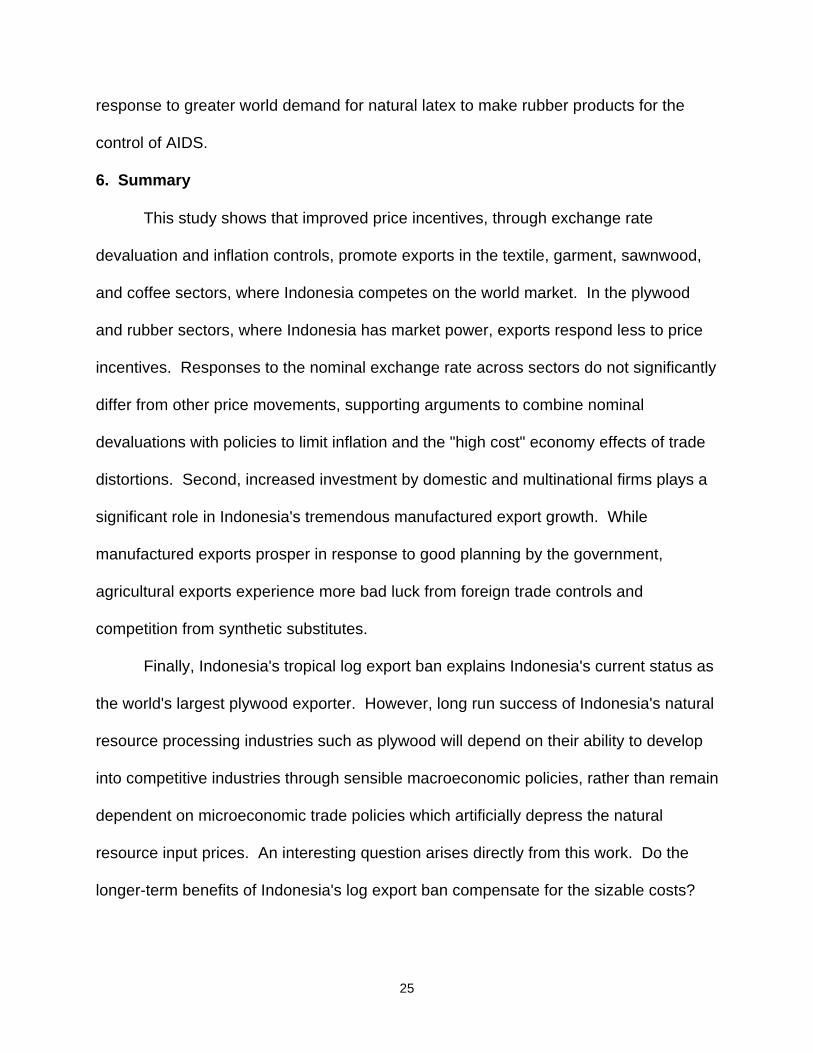
Appendix C1: Sectoral Elasticity Estimates, 1975-1990

Panel A: Textiles Structural Supply Panel B: Garments Structural Supply Panel C: Test Statistics Constrained Unconstrained Constrained Unconstrained Textiles Constrained Unconstrained

PX*ER/PDt 2.139 *** ERt 2.413 *** PX*ER/PDt 0.724 * ERt 0.336 Sample size 64 64 (0.548) (0.666) (0.413) (0.525) SE 0.359 0.360FXt 0.863 *** PX/PDt 1.452 FXt 0.010 PX/PDt 1.446 * Adj. R2 0.881 0.875 (0.292) (1.007) (0.321) (0.731) F 78.606 64.094YTt 1.957 *** FXt 0.873 *** FXt-1 0.214 FXt 0.156 DW 1.783 1.796 (0.368) (0.297) (0.210) (0.343)Constant -18.507 *** YTt 1.495 ** FXt-2 0.274 FXt-1 0.148 Garments Constrained Unconstrained (1.943) (0.702) (0.211) (0.215)p 0.494 *** Constant -24.422 *** FXt-3 0.189 FXt-2 0.131 Sample size 61 61 (0.114) (6.324) (0.288) (0.242) SE 0.230 0.229 p 0.506 *** EFXt-i 0.686 FXt-3 0.105 Adj. R2 0.957 0.959 (0.114) (0.418) (0.295) F 123.823 117.020 YTt 1.686 *** EFXt-i 0.540 DW 1.978 1.993 (0.322) (0.432) Degree PDL 2 2 POILt 0.685 * YTt 2.030 *** (0.376) (0.431) D83-90 3.830 ** POILt 0.762 ** (1.775) (0.377) D*POILt -0.823 ** D83-90 4.151 ** (0.363) (1.777) Constant -12.939 *** D*POILt -0.908 ** (1.271) (0.366) p 0.297 ** Constant -18.904 *** (0.135) (3.535) p 0.289 ** (0.138)

Notes: Significance levels: *** = 1%, ** = 5%, * = 10% (two tail tests). The parentheses contain standard errors. The dependent variable (X )it

equals sector i's export quantity in period t. The variable PX denotes sector i's dollar export price, ER denotes the nominal exchange ratet t

(rupiah/US$), PD denotes sector i's domestic price level, FX denotes foreign exchange availability, YT denotes trend domestic income, POILt t t t

denotes the world oil price, and D83-90 denotes a dummy for the 1983-90 policy reforms.

Test Results: In Panel A, the P Hausman test statistic for the endogeneity of PX equals 3.243, and for PD equals 2.629. Neither are2t t

significant at the 10% level or better. Coefficients on PX and PD do not significantly differ from each other (t=0.930). Coefficients ont t

PX/PD and ER do not significantly differ from each other (t=0.790). The variable PD has high correlation with PX (0.972) and with YTt t t t t

(0.986). In Panel B, the P Hausman test statistic for the endogeneity of PX equals 1.249, and for PD equals 5.702. Neither are significant at2t t

the 10% level or better. Coefficients on PX and PD do not significantly differ from each other (t=1.107). Coefficients on PX/PD and ER dot t t t

not significantly differ from each other (t=1.194). The variable PD has high correlation with PX (0.976) and with YT (0.984). See Appendix C3t t t

for estimation procedure.

31

Appendix C2: Sectoral Elasticity Estimates, 1975-1990

Panel A: Plywood Reduced Form Panel B: Sawnwood Structural Supply Panel C: Test Statistics Constrained Unconstrained Constrained Unconstrained Plywood Constrained Unconstrained

ER/PDt 2.120 *** ERt 2.116 *** PX*ER/PDt 0.364 *** ERt -0.543 Sample size 60 60 (0.488) (0.429) (0.106) (0.499) SE 0.313 0.342ER/PDt-1 -0.367 ERt-1 -0.766 PX*ER/PDt-1 0.365 *** ERt-1 0.333 Adj. R2 0.971 0.966 (0.481) (0.504) (0.104) (0.532) F 154.704 119.596ER/PDt-2 0.182 ERt-2 0.110 EPX*ER/PDt-i 0.729 *** EERt-i -0.210 DW 1.685 1.704 (0.321) (0.277) (0.127) (0.587) Degree PDL 3 3ER/PDt-3 0.559 ERt-3 0.828 ** FXt -0.214 PX/PDt 0.356 *** (0.501) (0.407) (0.241) (0.105) Sawnwood Constrained UnconstrainedER/PDt-4 -2.446 *** ERt-4 -2.530 *** FXt-1 0.348 ** PX/PDt-1 0.385 *** (0.503) (0.475) (0.157) (0.103) Sample size 61 61EER/PDt-i 0.047 EERt-i -0.242 FXt-2 0.506 *** EPX/PDt-i 0.741 *** SE 0.193 0.190 (0.314) (0.585) (0.166) (0.121) Adj. R2 0.624 0.648FXt -0.745 ** PDt -0.793 FXt-3 0.259 FXt -0.120 F 8.795 8.308 (0.321) (0.552) (0.267) (0.256) DW 1.777 1.740YWt 2.793 *** FXt -0.860 ** EFXt-i 0.900 *** FXt-1 0.220 Degree PDL 2 2 (0.652) (0.398) (0.329) (0.168) on FXPCOMPt 5.275 *** YWt 6.026 *** YTt 0.837 FXt-2 0.330 * (0.644) (1.531) (0.517) (0.196)PLOGt -0.120 PCOMPt 4.598 *** D80-85 -0.285 * FXt-3 0.207 (0.465) (0.767) (0.154) (0.317)D80-85 7.554 *** PLOGt -0.113 D90 -1.088 *** EFXt-i 0.636 * (2.780) (0.579) (0.190) (0.361)D*PLOGt -1.378 ** D80-85 7.981 ** Constant -6.688 *** YTt 3.722 ** (0.594) (3.308) (2.434) (1.850)Constant -30.208 *** D*PLOGt -1.417 ** p 0.644 *** D80-85 -0.245 (2.474) (0.698) (0.121) (0.159) Constant -36.661 *** D90 -1.164 *** (3.992) (0.187) Constant -17.831 *** (5.183) p 0.598 *** (0.132)

Notes: Significance levels: *** = 1%, ** = 5%, * = 10% (two tail tests). The parentheses contain standard errors. The dependent variable (X )it

equals sector i's export quantity in period t. The variable PX denotes sector i's dollar export price, ER denotes the nominal exchange ratet t

(rupiah/US$), PD denotes sector i's domestic price level, FX denotes foreign exchange availability, YW denotes world income, YT denotest t t t

trend domestic income, PCOMP denotes competitor country costs, PLOG denotes Indonesia's log price, D80-85 denotes a dummy for the 1980-85t t

progressive log export ban, and D90 denotes a dummy for the 1990 sawnwood export tax.

Test Results: In Panel A, the P Hausman test statistic for the endogeneity of PX in the structural supply equation equals 27.850, significant2t

at the 1% level. Lags on PD are insignificant; to limit the number of regressors I do not add them to the final equation. The variables YTt t

and YW have high correlation (0.997), so I only add YW . In Panel B, the P Hausman test statistic for endogeneity of PX equals 5.791, and fort t t2

PD equals 2.789. Neither are significant at the 10% level or better. Coefficients on PX/PD and ER do significantly differ from each othert t t

(t=1.865), but coefficients on PX/PD and ER do not (t=0.100). The variable PD has high correlation with YT (0.958). See Appendix C3 fort-1 t-1 t t

estimation procedure.

32

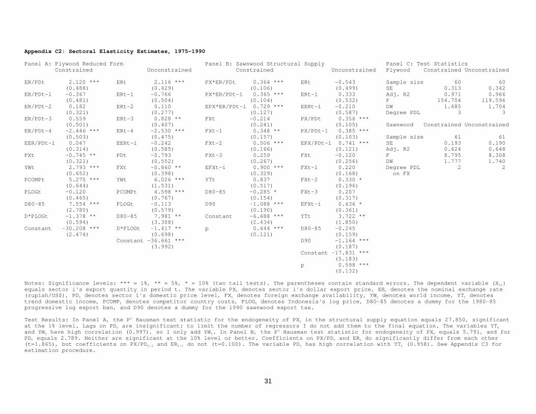
Appendix C3: Sectoral Elasticity Estimates, 1975-1990

Panel A: Coffee Structural Supply Panel B: Rubber Reduced Form Panel C: Test Statistics Constrained Unconstrained Constrained Unconstrained Coffee Constrained Unconstrained

PX*ER/PDt -0.149 ERt 0.123 ER/PDt -0.131 * ERt 0.191 ** Sample size 62 62 (0.125) (0.195) (0.072) (0.095) SE 0.179 0.175PX*ER/PDt-1 0.098 *** ERt-1 0.004 FXt 0.089 PDt 0.126 ** Adj. R2 0.803 0.812 (0.027) (0.063) (0.125) (0.057) F 28.650 24.891PX*ER/PDt-2 0.345 *** ERt-2 -0.116 YWt 0.585 *** FXt 0.175 DW 2.059 2.238 (0.114) (0.209) (0.156) (0.122) Degree PDL 1 1EPX*ER/PDt-i 0.294 *** EERt-i 0.012 PCOMPt 0.026 YWt 0.023 (0.082) (0.191) (0.283) (0.237) Rubber Constrained UnconstrainedFXt 0.219 *** PX/PDt -0.188 POILt -0.189 *** PCOMPt -0.085 (0.071) (0.125) (0.065) (0.279) Sample size 64 64YTt 2.151 *** PX/PDt-1 0.093 *** D83-90 -0.803 ** POILt -0.216 *** SE 0.084 0.079 (0.163) (0.029) (0.330) (0.071) Adj. R2 0.705 0.737D77 -0.182 * PX/PDt-2 0.373 *** D*POIL 0.202 *** D83-90 -1.116 *** F 16.060 17.026 (0.103) (0.111) (0.073) (0.322) DW 1.720 1.880D80-89 -0.206 *** EPX/PDt-i 0.278 *** Constant 2.660 *** D*POIL 0.256 *** (0.045) (0.086) (0.675) (0.068) Constant -7.748 *** FXt 0.202 *** Constant 3.481 *** (1.091) (0.076) (0.538) YTt 2.932 *** (0.625) D77 -0.172 * (0.103) D80-89 -0.211 *** (0.041) Constant -11.278 *** (2.401)

Notes: Significance levels: *** = 1%, ** = 5%, * = 10% (two tail tests). The parentheses contain standard errors. The dependent variable (X )it

equals sector i's export quantity in period t. The variable PX denotes sector i's dollar export price, ER denotes the nominal exchange ratet t

(rupiah/US$), PD denotes sector i's domestic price level, FX denotes foreign exchange availability, YT denotes trend domestic income, YWt t t t

denotes world income, D77 denotes a dummy for the 1977 world coffee price surge, D80-89 denotes a dummy for the International CoffeeAgreement, PCOMP denotes competitor country costs, POIL denotes the world oil price (proxy for the synthetic rubber price), and D83-90t t

denotes a dummy for the 1983-90 period.

Test Results: In Panel A the P Hausman test statistic for the endogeneity of PX equals 11.679, and for PD equals 4.824. Neither are2t t

significant at the 10% level or better. Coefficients on PX/PD and ER and on PX/PD and ER do not significantly differ from each othert t t-1 t-1

(t=1.350,0.832), but coefficients on PX/PD and ER do (t=2.090). The variable PD has high correlation with YT (0.926). In Panel B the Pt-2 t-2 t t2

Hausman test statistic for the endogeneity of PX in the structural supply equation equals 26.422, significant at the 1% level. The variablest

YT and YW have high correlation (0.997), so I only add YW . Coefficients on ER and PD do not significantly differ from each other (t=0.510).t t t t t

Estimation: I make corrections for seasonality with quarterly dummies but do not report them. I estimate regressions with an Almon lag onprices and foreign exchange; choose lag lengths by minimizing Akaike's final prediction error criterion with the constraint of 4 quartersmaximum lag; choose the polynomial degrees following Johnston (1984,p.354-5); and test the coefficients for optimality with likelihood ratiotests. I re-estimate equations with the Cochrane-Orcutt (CO) iterative technique if the Durbin Watson statistic falls below the critical uppervalue; Appendix C reports estimates for the autocorrelation coefficient D. The OLS regressions use a heteroskedasticity consistent covariancematrix.

33

References

Akiyama, T. and P. Verangis, 1990, The impact of the international coffee agreementon producing countries, The World Bank Economic Review 4(2), 157-173.

Arize, A., 1990, An econometric investigation of export behavior in seven Asiandeveloping countries, Applied Economics 22(7), 891-904.

Athukorala, P., 1991, Exchange rate pass-through: The case of Korean exports of manufactures, Economics Letters 35(1), 79-84.

Bahmani-Oskooee, M., 1986, Determinants of international trade flows, Journal ofDevelopment Economics 20(1), 107-123.

Barichello, R. and F. Flatters, 1991, Trade policy reform in Indonesia, in: D. Perkins andM. Roemer, eds., Reforming economic systems in developing countries (HarvardUniversity Press, Cambridge, MA) 271-291.

Bond, M., 1985, Export demand and supply for groups of non-oil developing countries,International Monetary Fund Staff Papers 32(1), 56-77.

Corbo, V. and P. McNelis, 1989, The pricing of manufactured goods during tradeliberalization: Evidence from Chile, Israel, and Korea, The Review of Economicsand Statistics 71(3), 491-499.

Devarajan, S., J. Lewis, and S. Robinson, 1991, External shocks, purchasing powerparity, and the equilibrium real exchange rate, Harvard Institute for InternationalDevelopment, Development Discussion Paper No. 385.

General Agreement on Tariffs and Trade, 1991, Trade policy review: Indonesia (GATT, Geneva).

Glassburner, B., 1988, Indonesia: Windfalls in a poor rural economy, in: A. Gelb, et.al.,Oil windfalls: Blessings or curse? (Oxford University Press for the World Bank,London) 197-226.

Goldstein, M. and M. Khan, 1976, Large versus small price changes and the demandfor imports, International Monetary Fund Staff Papers 23(1), 200-225.

Goldstein, M. and M. Khan, 1978, The supply and demand for exports: A simultaneousapproach, The Review of Economics and Statistics 60(2), 275-286.

Goldstein, M. and M. Khan, 1985, Income and price effects in foreign trade, in: R.Jones and P. Kenen, eds., Handbook of international economics, Vol.2 (North-Holland, Amsterdam) 1041-1105.

Hill, H., 1991, The emperor's clothes can now be made in Indonesia, Bulletin ofIndonesian Economic Studies 27(3), 89-127.

Hong Kong Census and Statistics Department, various issues, Hong Kong monthlydigest of statistics.

International Monetary Fund, various issues, International financial statistics, (IMF,Washington, DC).

Johnston, J., 1984, Econometric methods, Third edition (McGraw-Hill Book Company, New York).

Kellman, M. and P. Chow, 1989, The comparative homogeneity of the East Asian NIC exports of similar manufactures, World Development 17(2), 267-273.

Kendall, M. and A. Stuart, 1977, The advanced theory of statistics, (MacMillanPublishing Co, Inc, New York).

34

Khan, M., 1974, Import and export demand in developing countries, InternationalMonetary Fund Staff Papers 21(3), 678-693.

Lazard Freres et Cie, Lehman Brothers, and S.G. Warburg & Co. Ltd., 1990, Therepublic of Indonesia (Mimeo).

Lindsay, H., 1989, The Indonesian log export ban: An estimation of foregone exportearnings, Bulletin of Indonesian Economic Studies 25(2), 111-123.

Lucas, R., 1988, Demand for India's manufactured exports, Journal of DevelopmentEconomics 29, 63-75.

Marquez, J. and C. McNeilly, 1988, Income and price elasticities for exports ofdeveloping countries, The Review of Economics and Statistics 70(2), 306-314.

Moran, C., 1988, A structural model for developing countries' manufactured exports,The World Bank Economic Review 2(3), 321-340.

Office of the United States Trade Representative, various issues, Foreign trade barriers(Department of Commerce, Washington, D.C.).

O'Neill, H. and W. Ross, 1991, Exchange rates and South Korean exports to OECDcountries, Applied Economics 23(7), 1227-1236.

Organization for Economic Cooperation and Development, various issues, Quarterlynational accounts (OECD, Paris).

Pitt, M., 1981, Alternative trade strategies and employment in Indonesia, in: A. Krueger,et.al., eds., Trade and employment in developing countries, Vol.1 (The Universityof Chicago Press, Chicago) 181-237.

Riedel, J., 1988, The demand for LDC exports of manufactures: Estimates from HongKong, The Economic Journal 98, 138-148.

Roemer, M., 1985, Dutch disease in developing countries: Swallowing bitter medicine,"in: M. Lundhal, ed., The primary sector in economic development (Croom Helms,London) 234-252.

Sundararajan, V., 1986, Exchange rate versus credit policy: Analysis with a monetarymodel of trade and inflation in India, Journal of Development Economics 20(1),75-105.

Tegene, A., 1989, On the effects of relative prices and effective exchange rates ontrade flows of LDC's, Applied Economics 21(11), 1447-1463.

Thorbecke, E., 1991, The Indonesian adjustment experience in an internationalperspective, Institute for Policy Reform Working Paper Series.

Thursby, J. and M. Thursby, 1984, How reliable are simple, single equationspecifications of import demand? The Review of Economics and Statistics 66(1),120-128.

United Nations, various issues, International trade statistics yearbook (UN, New York).Warner, D. and M. Kreinin, 1983, Determinants of international trade flows, The

Review of Economics and Statistics 65(1), 96-104.Wilson, J. and W. Takacs, 1979, Differential responses to price and exchange rate

influences in the foreign trade of selected industrial countries, The Review ofEconomics and Statistics 61(2), 267-279.

Woo, W. and A. Nasution, 1989, Indonesian economic policies and their relation toexternal debt management, in: J. Sachs and S. Collins, eds., Developing countrydebt and economic performance, Vol.3 (The University of Chicago Press,Chicago) 17-149.

35

World Bank, various issues, World debt tables (The World Bank, Washington, D.C.).World Bank, 1992, World development report 1992 (Oxford University Press, New

York).World Bank, various issues, World tables (The Johns Hopkins University Press,

Baltimore, MD).

36

Table 1: Indonesian Macroeconomic Indicators, 1970-1990

Panel A: Average Levels in Sub-Periods 1970-72 1973-78 1979-81 1982-85 1986-90

Population 122.5 134.4 147.3 159.8 174.9 (millions)GDP/Capita 80.4 254.8 486.3 555.8 504.1 (US$)Exchange Rate 389.9 419.5 627.3 926.8 1645.0 (rp/$)Real Exchange 85.4 67.2 82.4 88.8 178.3 Rate IndexMoney Market na 10.7 14.1 14.8 13.9 Interest Rate

Panel B: Average Annual Rates of Change in Sub-Periods 1970-72 1973-78 1979-81 1982-85 1986-90

Indonesian 8.0% 7.9% 8.0% 4.0% 6.3% Real GDPAsian 6.9% 6.1% 5.2% 6.9% 7.1% Real GDP Consumer Price 7.8% 21.7% 15.5% 9.1% 7.4% IndexMoney + Quasi 44.1% 33.2% 36.8% 24.5% 29.9% MoneyOil Price 22.2% 43.2% 39.2% -5.6% -2.4%

Panel C: Average Annual Ratios in Sub-Periods 1970-72 1973-78 1979-81 1982-85 1986-90

Debt Service 17.4% 16.6% 15.9% 22.5% 40.7% /ExportsTotal Debt 306.2% 152.6% 101.9% 145.7% 266.8% /ExportsDebt Service 2.4% 3.8% 4.7% 5.3% 9.1% /GDPTotal Debt 42.2% 35.2% 30.0% 34.2% 59.3% /GDPTotal Exports 13.8% 23.5% 29.3% 23.7% 22.3% /GDPNonoil Exports 7.8% 7.5% 8.0% 5.9% 12.2% /GDPTotal Imports 12.3% 14.9% 14.5% 16.1% 16.6% /GDPCurrent Account -3.5% -1.6% 1.8% -4.3% -2.7% /GDPGov Expenditures 15.1% 21.2% 25.0% 22.9% 22.1% /GDPGov Revenues 11.8% 17.4% 21.5% 19.0% 16.4% /GDP

Notes: Real Asian GDP equals an average for 19 Asian LDCs; money market ratefor 1970-74 not available; real exchange rate base year 1985; imports andexports constitute merchandise trade only. Government budget figures coverfiscal years.

Sources: Indonesian Bureau of Statistics; The World Bank, World Debt Tablesand World Tables; International Monetary Fund, International FinancialStatistics; Woo and Nasution (1989); Lazard Freres et Cie (1990).

37

Table 2: Overview of Policy Changes, 1970-1990

Micro Restriction: 1970-81 Mixed Signal: 1982-85 Steady Reform: 1986-90

Exchange * Unify, devalue, and fix * Devalue 39% in March 1983 * Devalue 33% in Sept. 1986Rate exchange rate, 415 Rp/$, 1971 from 698 Rp/$ to 970 Rp/$ ++ from 1232 Rp/$ to 1644 Rp/$ ++ * Devalue 48% in Nov. 1978 * Lift requirement for exporters * Improve Central Bank's foreign from 415 Rp/$ to 614 Rp/$ ++ to sell all foreign exchange exchange swap mechanism * Change from fixed rate earnings to Central Bank * Allow free capital movements regime to managed float with * Allow free capital movements periodic devaluations * Allow free capital movements

Trade * Increase tariff and * Increase non-tariff * Compensate some producers and Restric- non-tariff barriers barriers to cover 1500 items importers with tariff protectiontions in Approved Importers Scheme

Sectoral * Begin to phase out * Ban all log exports * Tax sawnwood exports Restric- log exports * Restrict batik, some steel, * Ban rattan and some sawnwood, rubbertions coal, and some food imports and leather export categories * Impose "temporary" import surcharges on some textiles, synthetic fibers, chemicals, iron & steel, and some foods

Trade * Introduce export subsidy * Start Counterpurchase Agreements * Remove half of non-tariff barriersPromotion program with foreign contractors * Further lower average tariff rates * Reduce interest rates * Lower average tariff rates and simplify tariff code on export credits * Simplify tariff code * Improve export subsidy program with * Remove some export taxes * Replace Indonesian Customs duty drawback system. Grants exporters with private foreign company rebates on import duties; exporters * Sign GATT Code on Subsidies may purchase imported inputs directly and Countervailing Duties, 1985 * Deregulate inter island shipping * Further lower interest rates on export credits * Improve port operations

Sectoral * Improve textile and garment quota Promotion allocation system * Simplify import procedures and remove non-tariff barriers for textiles, cotton, machinery & equipment, electrical products, and some steel products * Lift restrictions on coffee exporters to join marketing groups++ Based on average quarterly exchange rates * Lift export restrictions on some (Table 2 continues on next page) agriculture products

38

Table 2: Overview of Policy Changes, 1970-1990

Micro Restriction: 1970-81 Mixed Signal: 1982-85 Steady Reform: 1986-90

Fiscal * Follow balanced budget * Cut expenditures on almost 50 * Add broad-based land & property tax policy; deficit covered by capital intensive projects * Continue balanced budgets foreign borrowing * Revise income tax code * Maintain punctual foreign * Maintain punctual foreign * Introduce 10% value added tax debt repayments debt repayments and sales tax on luxury goods * Invest heavily in agricul- * Continue balanced budgets tural infrastructure and * Maintain punctual foreign subsidies debt repayments

Industrial * Require all foreign * Increase local content rules * Relax local ownership requirements, investment in joint ventures especially capital intensive projects * Close sectors to investment * Open sectors to investment and * Impose local content laws introduce simplified "Negative List" of closed sectors * Simplify licensing procedures * Develop new industrial estates and bonded trade zones * Improve infrastructure * Ease foreign employment restrictions

Financial * Abolish all credit ceilings * Introduce auction and secondary * Permit state banks to set market for Central Bank instruments interest rates * Phase out liquidity credit scheme * Reduce subsidized credit * Reduce foreign bank restrictions from Central Bank * Simplify bank branch establishment * Introduce Central Bank and * Lessen bank restrictions to money market instruments deal in foreign exchange * Cut special privileges of state owned financial institutions * Lower the reserve requirement * Allow parallel securities market * Enlarge scope of rural banks * Clarify capital market regulations * Abolish securities price controls * Establish procedures for new stock issues and licensing of brokers * Permit foreign investors to buy up to 49% of listed issues Sources: General Agreement on Tariffs and Trade (1991); Lazard Freres et.al. (1990); Office of the United States TradeRepresentative (various issues); Woo and Nasution (1989).

39

Table 3: Regional Comparison of Export Compositions and Growth, 1970-1990

Panel A: Average Annual Manufactured Export Shares in Total Exports 1970-72 1973-78 1979-81 1982-85 1986-90

Indonesia 1.7% 1.6% 2.8% 8.0% 28.1%Korea 80.6% 85.3% 89.8% 91.3% 92.7%Malaysia 9.1% 15.6% 19.0% 25.5% 41.7%Philippines 8.0% 21.6% 38.8% 53.0% 60.8%Thailand 11.6% 19.0% 26.9% 33.1% 54.1%

Panel B: Average Annual Oil Export Shares in Total Exports 1970-72 1973-78 1979-81 1982-85 1986-90

Indonesia 43.0% 67.0% 73.0% 75.1% 45.6%Korea 1.1% 1.5% 0.4% 2.3% 1.4%Malaysia 8.2% 11.3% 23.2% 29.7% 18.0%Philippines 1.6% 0.9% 0.5% 1.2% 1.9%Thailand 0.8% 0.5% 0.0% 0.4% 0.8%

Panel C: Average Annual Real Non-Oil Export Growth 1970-72 1973-78 1979-81 1982-85 1986-90

Indonesia 6.2% 15.8% -4.2% 5.5% 17.2%Korea 34.1% 28.5% 6.0% 7.3% 14.2%Malaysia -2.6% 14.5% -1.1% 4.2% 15.5%Philippines -4.9% 10.8% 6.8% -6.5% 10.6%Thailand 17.9% 14.2% 6.9% -0.8% 23.8%

Panel D: Average Annual Real Manufactured Export Growth 1970-72 1973-78 1979-81 1982-85 1986-90

Indonesia 51.0% 23.0% 32.3% 28.1% 31.4%Korea 40.3% 29.5% 7.0% 8.2% 14.2%Malaysia 18.9% 27.0% 6.1% 14.5% 21.8%Philippines 4.5% 37.2% 17.8% -0.8% 12.8%Thailand 65.6% 22.2% 11.8% 8.7% 36.7%

Notes: The table calculates average annual growth rates from real exportrevenues in 1985 U.S. dollars. The annual U.S. producer price index equalsthe non-oil export earnings deflator.

Sources: Indonesian Bureau of Statistics; The World Bank, World Tables,International Monetary Fund, International Financial Statistics.

40

Table 4: Average Annual Real Export Revenue Growth, 1975-1990

1975-78 1979-81 1982-85 1986-90 ------------------------------------------------Oil and Gas 11.9% 0.1% -6.9% 2.3% Oil 9.3% -1.8% -11.6% 0.9% Gas -- 21.0% 15.5% 5.3%

Non-Oil Exports 19.4% -4.2% 5.5% 17.2%

Agriculture 21.3% -10.0% 5.6% 4.8% Rubber 18.4% -6.0% -4.9% 1.1% Fish & Shrimp 21.8% -7.0% 2.2% 29.9% Coffee 60.2% -20.4% 11.3% -9.8% Veg. Oils 3.8% -24.5% 32.1% -2.1% Tea,Spices,Cocoa 24.2% -8.4% 10.9% 3.5% Other Ag 6.5% 2.2% 5.5% 9.3%

Mining & Wood 15.7% -4.8% -11.9% 5.3% Sand,Clay,Coal -5.7% 52.4% 38.0% 26.8% Tin 47.5% 3.9% -15.2% -8.6% Aluminum 4.3% 36.5% 350.7% -5.3% Metal Ores -17.4% 28.7% -7.5% 17.3% Logs 17.3% -19.7% -68.5% -100.0% Sawnwood 31.1% 21.5% -0.1% 0.9%

Manufactures 28.9% 32.4% 28.1% 31.4% Plywood 165.0% 81.0% 45.7% 23.3% Textiles&Garments 58.5% 64.8% 43.0% 34.7% Footwear 60.8% 25.3% 25.8% 129.7% Chemicals 23.8% -6.1% 32.8% 21.3% Machinery&Equip. 22.5% 15.8% -11.8% 27.1% Other 19.9% 33.8% 4.8% 45.2%======================================================================Total Exports 13.6% -0.9% -3.7% 7.9%

Notes: The table calculates average annual growth rates from real exportrevenues in 1985 U.S. dollars. The annual U.S. producer price index equalsthe non-oil export earnings deflator, and the official Indonesian oil priceequals the oil export earnings deflator. Metal ores include other metals.

Source: Trade data from Indonesian Bureau of Statistics; price deflators fromInternational Monetary Fund, International Financial Statistics.

41

Table 5: Comparison of Almon Lag and Partial Adjustment Long Run Estimates

Structural Supply |Reduced Form Textiles Garments Sawnwood Coffee |Plywood Rubber |PX*ER/PD |ER/PDAlmon 2.139 *** 0.724 * 0.729 *** 0.294 ***| 0.047 -0.131 * (0.548) (0.413) (0.127) (0.082) | (0.314) (0.072)Part Adj 2.662 * 0.530 0.775 *** 0.139 | 0.873 -0.169 * (1.586) (0.677) (0.265) (0.120) | (2.266) (0.093) |FX |FXAlmon 0.863 *** 0.686 0.900 *** 0.219 ***| -0.745 ** 0.089 (0.292) (0.418) (0.329) (0.071) | (0.321) (0.125)Part Adj 0.968 0.409 0.505 0.230 ***| 0.678 0.118 (0.662) (0.543) (0.399) (0.080) | (1.391) (0.157) |YT |YWAlmon 1.957 *** 1.686 *** 0.837 2.151 ***| 2.793 *** 0.585 *** (0.368) (0.322) (0.517) (0.163) | (0.652) (0.156)Part Adj 1.610 1.715 0.670 2.062 ***| 1.634 0.615 ** (1.442) (1.619) (0.722) (0.627) | (3.730) (0.266) | n Almon 64 61 61 62 | 60 64 n Part Adj 63 63 63 63 | 63 63dof Almon 60 51 51 54 | 48 56dof Part Adj 58 55 56 56 | 54 54

Significance levels: *** = 1%, ** = 5%, * = 10% (two tail tests). See AppendixC for Almon lag results and Appendix B for explanation of partial adjustmentapproach. The letter n denotes sample size and dof denotes degrees of freedom.

Table 6: Summary of Price and Exchange Rate Estimates (Almon Lag) Structural Supply |Reduced Form Textiles Garments Sawnwood Coffee |Plywood Rubber |Panel A: Constrained Price |PX*ER/PD |ER/PD 2.139 *** 0.724 * 0.729 *** 0.294 ***| 0.047 -0.131 * (0.548) (0.413) (0.127) (0.082) | (0.314) (0.072) |Panel B: Unconstrained Price |ER |ER 2.413 *** 0.336 -0.210 0.012 | -0.242 0.191 ** (0.666) (0.525) (0.587) (0.191) | (0.585) (0.095) |PX/PD |PD 1.452 1.446 * 0.741 *** 0.278 ***| -0.793 0.126 ** (1.007) (0.731) (0.121) (0.086) | (0.552) (0.057) |n 64 61 61 62 | 60 64dof A 60 51 51 54 | 48 56dof B 59 50 49 51 | 47 55

Significance levels: *** = 1%, ** = 5%, * = 10% (two tail tests). See AppendixC. The letter n denotes sample size and dof denotes degrees of freedom.

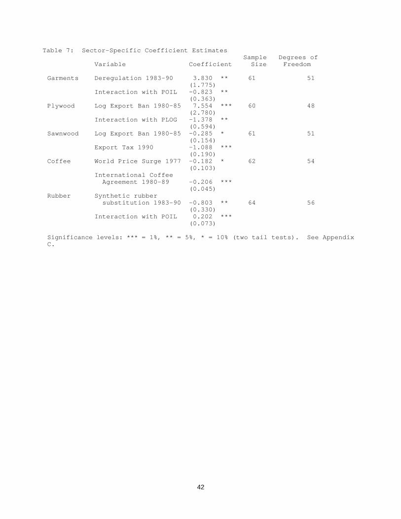
42

Table 7: Sector-Specific Coefficient Estimates Sample Degrees of

Variable Coefficient Size Freedom

Garments Deregulation 1983-90 3.830 ** 61 51(1.775)

Interaction with POIL -0.823 **(0.363)

Plywood Log Export Ban 1980-85 7.554 *** 60 48(2.780)

Interaction with PLOG -1.378 **(0.594)

Sawnwood Log Export Ban 1980-85 -0.285 * 61 51(0.154)

Export Tax 1990 -1.088 ***(0.190)

Coffee World Price Surge 1977 -0.182 * 62 54(0.103)

International Coffee Agreement 1980-89 -0.206 ***

(0.045)Rubber Synthetic rubber

substitution 1983-90 -0.803 ** 64 56(0.330)

Interaction with POIL 0.202 ***(0.073)

Significance levels: *** = 1%, ** = 5%, * = 10% (two tail tests). See AppendixC.

0

1

2

3

4

5

6

7

8

9

Plywood Textiles & Garments Footwear

Chemicals Machinery & Equipment Other Manufactures

1975 1976 1977 1978 1979 1980 1981 1982 1983 1984 1985 1986 1987 1988 1989 1990

Figure 2: Composistion of Manufactured Export Earnings (in constant 1985 US$)

0

5

10

15

20

25

30

Agriculture Mining & WoodManufactures Oil & Gas

1975 1976 1977 1978 1979 1980 1981 1982 1983 1984 1985 1986 1987 1988 1989 1990

Figure 1: Composition of Total Export Earnings (in constant 1985 US$)

0

1

2

3

4

5

Rubber Fish & Shrimp Coffee

Vegetable Oils Tea,Spices,Cocoa Other Agriculture

1975 1976 1977 1978 1979 1980 1981 1982 1983 1984 1985 1986 1987 1988 1989 1990

0

500

1000

1500

2000

2500

3000

3500

Sand,Clay,Coal Tin AluminumMetal Ores Logs Sawnwood

1975 1976 1977 1978 1979 1980 1981 1982 1983 1984 1985 1986 1987 1988 1989 1990

Figure 3: Composition of Mining & Wood Export Earnings (in constant 1985 US$)

Figure 4: Composistion of Agricultural Export Earnings (in constant 1985 US$)