Development and application of otolith- based methods to...
230
Development and application of otolith- based methods to infer demographic connections in a marine metapopulation by Philipp Neubauer A thesis submitted to Victoria University of Wellington in fulfilment of the requirements for the degree of Doctor of Philosophy in Marine Biology Victoria University of Wellington 2012
Transcript of Development and application of otolith- based methods to...
Development and application of otolith-
based methods to infer demographic
connections in a marine
metapopulation
by
Philipp Neubauer
A thesis submitted to
Victoria University of Wellington
in fulfilment of the requirements for the degree of
Doctor of Philosophy in Marine Biology
Victoria University of Wellington
2012

This thesis has been conducted under the supervision of:
Dr. Jeffrey S. Shima (Primary Supervisor)
Victoria University of Wellington
Wellington, New Zealand
and
Dr. Steven E. Swearer (Secondary Supervisor)
University of Melbourne
Melbourne, Australia


v
To my family,
for past, present
and future.

ii
iii
Abstract
Connectivity between local populations is critical if these are to
function as a metapopulation and sustain locally open sink populations.
Assessing whether such connections between local populations exist is
thus an important step towards understanding coastal metapopulation
dynamics as well as assessing the efficacy of spatial management tools
such as marine reserve networks. For this thesis, I investigate population
connectivity of the common triplefin (Forsterygion lapillum) in Cook Strait,
New Zealand, using chemical signatures contained within fish otoliths (ear
stones). I concentrate on likely connections between three local marine
reserves: Kapiti Island (Kapiti coast), Long Island (Marlborough Sounds) and
Taputeranga Marine Reserve (Wellington south coast). To this end I
develop and implement new statistical methods to enable stronger
inferences from otolith chemistry based approaches.
In chapter 2, I evaluate otolith core chemistry as a potential tool (i.e.
an environmental fingerprint) for identification of natal source populations
of the common triplefin. I sampled otolith chemistry from hatchling fish
across a range of hierarchical scales: obtained from individual egg masses
within a site; sites within different regions; and regions distributed on the
two main islands of New Zealand (North and South Island). This sampling
enabled me to construct an “atlas” (or baseline) of otolith core chemistry. I
developed and applied a set of novel statistical approaches to examine the
characteristics of this natal atlas and optimize its spatial resolution. These
analyses allowed me to assess the utility of otolith chemistry as a potential
tool to infer patterns of population connectivity in the vicinity of Cook
Strait.
Chapter 3 develops a new Bayesian approach to facilitate improved
clustering and classification of dispersing fish to putative natal populations
based on their otolith chemistry. Otolith-based approaches used to infer
iv
natal origins of fishes routinely suffer from the (unrealized) requirement to
sample all potential natal source populations. An incomplete baseline atlas
has greatly limited the application of otolith chemistry as a tool for
assessments of connectivity in the marine environment. In this chapter, I
develop, evaluate, and implement statistical solutions to this problem.
Specifically, I present a clustering model, based on infinite mixtures, which
does not require the specification of a potential number of sources. In a
second step, I embed this clustering model in a large-scale classification
model that allows for classification on scales encompassing a number of
potential sources, where recruits are clustered with observations from the
baseline or a separate cluster within these regions. This opens the
potential for fish that came from an identifiable source other than those
sampled to not be assigned to a sampled source. I evaluate the strength of
this approach using the well-known weakfish (Cynoscion regalis) dataset.
In chapter 4, I apply the statistical methods developed in chapter 3 to
the common triplefin. I sampled recent recruits of the common triplefin
within each of three marine reserves (Kapiti, Long Island, and Taputeranga)
and used otolith chemistry to infer probable natal origins. I then compare
these inferred patterns of connectivity with those predicted by a set of
hydrodynamic simulations. This comparison enabled me to (qualitatively)
assess the likelihood of connectivity (as predicted by otolith chemistry)
given local hydrodynamic conditions.
For chapter 5, I extend the Bayesian modelling approaches developed
in previous chapters to incorporate otolith chemistry data sampled from
throughout the life-history of dispersers. As in chapter 3, I develop and
evaluate the utility of this approach using a previously published data set
(Chinook salmon), and I apply the approach to the common triplefin in a
subsequent chapter. Specifically, I propose flexible formulations based on
latent state models, and compare these in a series of illustrative
simulations and an application to Chinook salmon contingent analysis.

v
In chapter 6, I apply the Bayesian framework (developed in chapter 5)
to the common triplefin data set. Specifically, I formulate a model based on
putative chemical distinctions between inshore and offshore water-
masses. This model allows me to compare dispersal histories among
recruits to a set of reserves (evaluated initially in chapter 4), and the
approach reveals patterns that appear to be common to all successful
recruits. I examine these findings in the light of results obtained in chapter
4 as well as local hydrodynamic conditions.
Finally, I conclude my thesis in chapter 7 by discussing the relevance
of my findings for the functioning of networks of sub-populations, both in a
metapopulation and a reserve network context.

vi

vii
Acknowledgements
I thank my supervisors, Jeff Shima and Steve Swearer for giving me the
opportunity to pursue my PhD, and for providing valuable and critical
assessment of my work, which helped me to develop my thinking and
writing in important ways.
This work wouldn’t have been possible without the continuous and
input and help from my dear friends and colleagues at the Victoria
University Coastal Ecology Laboratory, and I wish to especially thank
Alejandro Perez-Matus for providing initial support when I first started out
and for sharing his knowledge of the system and of fish biology in general.
The statistical developments in this thesis were influenced and
supported by a number of friends and colleagues. I especially thank Sergio
Hernandez for introducing me to mixture models and for discussing geeky
concepts such as fuzzy clustering and Dirichlet processes with me. My visit
with Babak Shababah helped me further develop these ideas, and I thank
him for his hospitality. Discussions with Michele Masuda, Russel Millar, as
well as with Jessica Miller and her lab-group at Oregon State University
proved useful in advancing the work presented in this thesis. I also thank
Jessica Miller and Simon Thorrold for sharing their data with me.
I am grateful to Shirley Pledger, Richard Arnold and Marcus Frean for
letting me sit in with their respective statistics and machine learning
classes, which helped me to make connections that I would not have made
otherwise. I also thank Marti Krcoçek and Mark Lewis for accepting me on
their ecological modelling course at Bamfield – the discussions with this
smart and fun group were invaluable. I am indebted to Bruce Menge and
the Pisco team at OSU for hosting me for extended periods and providing
me with a welcoming and enriching environment to work on this thesis.

viii
I am incredibly thankful to my amazing wife and love of my life, Emilie
Fleur, for making this the most eventful and unforgettable time of my life.
Her support and criticism are my drive to become a better scientist and a
wiser person. This thesis would not have been possible without her loving
encouragements.
9
Contents
Abstract .................................................................................. iii
Acknowledgements ............................................................... vii
List of Figures ........................................................................ xv
List of Tables ......................................................................... xix
1. General Introduction ......................................................... 1
1.1 Marine populations, their spatial scale and structure ......................... 1
1.1.1 Connectivity of marine populations and the open-closed
debate .................................................................................................. 2
1.1.2 Connectivity and management of marine resources ............... 4
1.2 Studying larval dispersal in the marine environment .......................... 6
1.2.1 Simulating demographic connectivity ...................................... 6
1.2.2 Empirical measures of demographic connectivity: from
evolutionary to ecological timescales .................................................... 8
1.2.3 Otolith Chemistry as a marker of natal origins ...................... 10
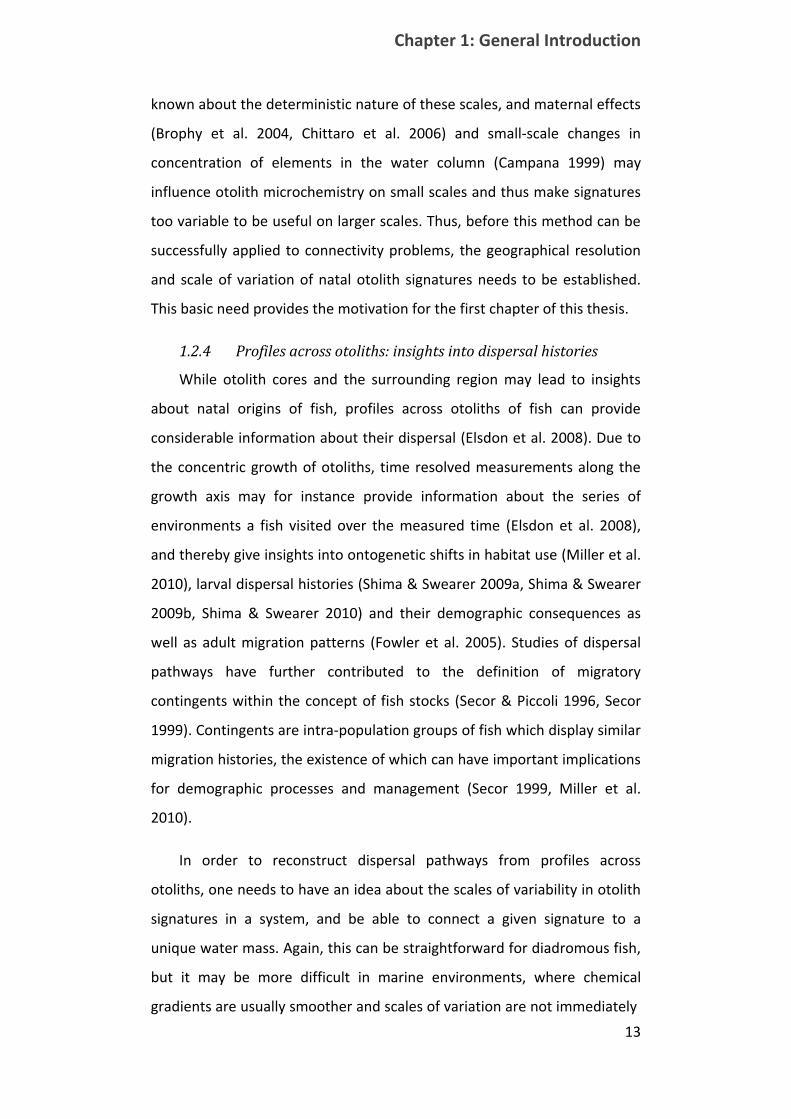
1.2.4 Profiles across otoliths: insights into dispersal histories ....... 13
1.3 Statistical methods for the analysis of otolith chemistry .................. 14
1.3.1 Bayesian methods for otolith chemistry ................................ 17
1.4 Contributions of this thesis ................................................................ 22
2. Scale-dependent variability in hatchling otolith chemistry: implications for studies of population * ................................. 27
2.1 Introduction ....................................................................................... 27
2.2 Methods ............................................................................................. 30
2.2.1 Study Species & Sampling ...................................................... 30
2.2.2 Otolith extraction, preparation and analysis ......................... 32
2.2.3 Statistical analysis .................................................................. 33
x
2.3 Results ................................................................................................ 38
2.3.1 Descriptive statistics, significance testing and discrimination...
................................................................................................ 38
2.3.2 Optimal grouping of sites by simulated annealing ................ 44
2.3.3 Exclusion test for groups of sites ........................................... 45
2.4 Discussion ........................................................................................... 47
2.4.1 Scaling of variability in hatchling otolith signatures .............. 47
2.4.2 Optimal regional groupings by SA .......................................... 49
2.4.3 Exclusion test ......................................................................... 50
2.4.4 Conclusion .............................................................................. 52
3. Characterizing natal sources of fish using flexible Bayesian mixture models for otolith geochemistry ............................... 53
3.1 Introduction ....................................................................................... 53
3.2 Statistical models ............................................................................... 58
3.2.1 A Dirichlet process mixture (DPM) model for clustering ....... 58
3.2.2 Using the DPM with a baseline .............................................. 62
3.2.3 Extension to hierarchical classification with an incomplete
atlas ................................................................................................ 64
3.2.4 Marginal descriptions of source assignments........................ 70
3.3 Application ......................................................................................... 71
3.3.1 DPM clustering models .......................................................... 71
3.3.2 Clustering fish without a baseline .......................................... 72
3.3.3 Clustering fish with a baseline ............................................... 75
3.3.4 Classification with a (potentially) incomplete baseline ......... 80
3.4 Discussion ........................................................................................... 85
4. Larval dispersal pathways in a reef fish metapopulation: Contrasting empirical and simulation measures..................... 89
xi
4.1 Introduction ....................................................................................... 89
4.2 Methods ............................................................................................. 92
4.2.1 Study system and otolith core chemistry atlas ...................... 92
4.2.2 Recruit otolith preparation and pre‐processing ................... 92
4.2.3 Selecting elements for analysis of otolith cores .................... 95
4.2.4 Statistical analysis of otolith chemistry.................................. 96
4.2.5 Simulation models of dispersal .............................................. 97
4.3 Results ................................................................................................ 99
4.3.1 Results from otolith microchemistry ..................................... 99
4.3.2 Results from hydrodynamic simulation experiments .......... 104
4.3.3 Comparing otolith and simulation results ................................ 111
4.4 Discussion ......................................................................................... 111
5. Plasticity and similarity in dispersal histories: a Bayesian framework for characterizing fish dispersal from otolith chemistry profiles ................................................................ 119
5.1 Introduction ..................................................................................... 119
5.2 Methods ........................................................................................... 123
5.2.1 Generative models for chemical transects .......................... 123
5.2.2 The Bayesian approach: Prior knowledge and the lack thereof
.............................................................................................. 128
5.2.3 Encoding alternate hypotheses ........................................... 129
5.2.4 Estimating the number of (distinguishable) environments
along a transect .................................................................................. 130
5.2.5 Temporal dynamics ............................................................. 132
5.2.6 Estimating unknowns: MCMC and WinBUGS ...................... 135
5.2.7 Characterizing contingents: a marginal visualization approach
.............................................................................................. 136
xii
5.3 Illustration and validation ................................................................ 137
5.3.1 Simulation Experiment I: Increasingly complex simulation
scenarios ............................................................................................ 138
5.3.2 Simulation Experiment II: Contingents from multivariate data .
.............................................................................................. 140
5.3.3 Assessing models: posterior predictive checks and model
selection ............................................................................................. 141
5.3.4 Application to Chinook salmon ............................................ 143
5.4 Results .............................................................................................. 145
5.4.1 Simulation experiment I ....................................................... 145
5.4.2 Simulation experiment II ...................................................... 148
5.4.3 Application to Chinook salmon ............................................ 150
5.5 Discussion ......................................................................................... 154
6. Inshore residency of fish larvae may maintain connections in a reef fish metapopulation .................................................. 161
6.1 Introduction ..................................................................................... 161
6.2 Methods ........................................................................................... 164
6.2.1 Recruit otolith preparation and pre‐processing ............... 164
6.2.2 Statistical model ................................................................... 164
6.2.3 Hydrodynamic model investigation ..................................... 168
6.3 Results .............................................................................................. 170
6.3.1 Results from models of dispersal histories ......................... 170
6.3.2 Hydrodynamic modelling results ......................................... 173
6.4 Discussion ......................................................................................... 176
6.4.1 Mixture model results for dispersal histories ...................... 176
6.4.2 Interpreting dispersal patterns ............................................ 179
6.4.3 Conclusions .......................................................................... 181

xiii
7. Discussion and perspectives .......................................... 183
Bibliography ........................................................................ 188
APPENDIX ............................................................................ 202
A.1 Weakfish exact linkage tree from the DPM clustering model ......... 202
A.2 Gibbs sampling in the mixture models ............................................ 203
A.3 Drawing a state sequence from the HMM – the recursive method 204
A.4 Winbugs code .................................................................................. 205

xiv

xv
List of Figures *
Figure 1.1: Left to right, picture of the head of a larval common triplefin
(Forsterygion lapillum) ................................................................................. 12
Figure 1.2: Picture of an adult common triplefin (Forsterygion lapillum) ... 23
Figure 1.3: A Coastal boundary layer in Cook Strait .................................... 25
Figure 2.1: Map of New Zealand and the sampling domain ....................... 31
Figure 2.2: Kernel smoothed histograms of trace element signatures from
the two main Islands along the linear discriminant function and regional
differences along the first two linear discriminant axes.............................. 41
Figure 2.3: Perspective plot showing predicted probability (p) of correct
assignment in a linear discriminant analysis in relation to number of groups
and inter-group Mahalanobis distance ........................................................ 43
Figure 2.4: Non-metric multi-dimensional scaling of sites within the total
sampling domain .......................................................................................... 44
Figure 2.5: Kernel-smoothed histograms (black) of Mahalanobis distances
to the centroid of the focal site ................................................................... 46
Figure 3.1: Illustration of the DPMc classification procedure (with a non-
fixed baseline for the DPM) ......................................................................... 67
Figure 3.2: Histogram of the marginal posterior distribution over the
number of sources in the weakfish baseline dataset. ................................. 74
Figure 3.3: Exact linkage tree from a self-assignment DPM analysis with
fixed baseline of weakfish juveniles. ............................................................ 76
Figure 3.4: Weakfish exact linkage tree from the DPM clustering model
with fixed baseline. ...................................................................................... 79
xvi
Figure 3.5: Exact linkage trees from the DPMc classification procedure .... 84
Figure 4.1 : Map of Cook Strait, New Zealand and the sampling domain ... 93
Figure 4.2: Hatchling atlas element distributions using a Bayesian approach
(Boxplot) ..................................................................................................... 102
Figure 4.3: Assignment summaries for fish collected at the three reserve
sites in Kapiti, Wellington and Long Island ................................................ 103
Figure 4.4: Comparison of log transformed signatures from samples in the
isolated cluster of Wellington sourced recruits vs. all other recruits
assigned to Wellington ............................................................................... 104
Figure 4.5: Tracers concentration 12h, 48h, 7 days and 14 days after being
released at sites around Kapiti Island ........................................................ 106
Figure 4.6: Tracers concentration 12h, 48h, 7 days and 14 days after being
released at sites on Wellington’s south coast. .......................................... 107
Figure 4.7: Tracers concentration 12h, 48h, 7 days and 14 days after being
released at sites in Wellington’s harbour. ................................................. 108
Figure 4.8: Tracers concentration 12h, 48h, 7 days and 14 days after being
released at sites in the Marlborough Sounds. ........................................... 109
Figure 4.9: Mean current velocities in Cook Strait predicted by the Gerris
flow solver ocean model ............................................................................ 110
Figure 4.10: Dispersal pathways inferred by otolith chemistry (arrows) .. 112
Figure 5.1: Example profiles for Strontium and Barium across Chinook
salmon otoliths ........................................................................................... 124
Figure 5.2: Directed acyclic graphs of the simple mixture model for
chemical transects across otoliths and the random effects mixture model
.................................................................................................................... 127

xvii
Figure 5.3: A hidden Markov model with individual transition matrices π for
each fish i ................................................................................................... 134
Figure 5.4: The 3x3 grid of (hypothetical and arbitrary) near-shore to
offshore variations in elemental concentration ........................................ 139
Figure 5.5: True and estimated partitions for a random effects mixture
model, a hidden Markov model (HMM) with a common transition matrix
and a HMM with individual matrices for each individual fish ................... 148
Figure 5.6: True and estimated partitions for a Dirichlet process random
effects mixture model, a mixture model with a single mixture proportion
over all fish and a hidden Markov model with a single transition matrix . 149
Figure 5.7: Marginal posterior distribution over the number of contributing
near-shore sources in simulation experiment II. ....................................... 149
Figure 5.8: Visualization of marginal similarity of transects from simulation
experiment II .............................................................................................. 151
Figure 5.9: Prior (dotted) versus posterior (line) distributions of water-mass
means of Strontium (Sr) and Barium for the three component model for
Chinook salmon .......................................................................................... 152
Figure 5.10: Histograms of the marginal posterior distribution over per cent
emigrating size classes and posterior distribution of size of Central
California Valley Chinook salmon at freshwater emigration. .................... 154
Figure 6.1: Example of three 138Ba:Ca traces and resulting density estimates
.................................................................................................................... 166
Figure 6.2: 6 hourly average wind direction and wind speed (in knots (kn))
at Wellington airport .................................................................................. 170
Figure 6.3: Modal estimated dispersal patterns of all fish at each site,
sorted by number of frames with inshore signatures ............................... 174

xviii
Figure 6.4: Visualization of Gerris simulation results of flow velocity ....... 175
Note that figure captions are abbreviated and/or slightly modified from
those in the text

xix
List of Tables *
Table 2.1: Distribution of trace element concentrations relative to
detection limits ............................................................................................ 40
Table 2.2: Variance explained and P values from nested permutational
MANOVA ...................................................................................................... 42
Table 2.3: Exclusion test results in per cent of hatchlings correctly excluded
from the focal location using full and truncated datasets ........................... 45
Table 3.1: Posterior expectation and mode for the number of sources in
each of four simulation experiment. ........................................................... 73
Table 3.2: Results from the assignment test ............................................... 78
Table 3.3: Comparison of the proportion Pc of correctly assigned individuals
in a self-assignment test for the weakfish and triplefin datasets ................ 82
Table 4.1: Distribution of trace element concentrations relative to
detection limits .......................................................................................... 101
Table 5.1: Simulation parameters for experiments I and II ....................... 140
Table 5.2: Prior parameters used for the Chinook salmon dataset ........... 145
Table 5.3: Simulation results for each simulated scenario ........................ 147
Table 6.1: Expectation and 95 per cent credible interval of the posterior
distribution of some parameters in the dispersal model .......................... 171
Table 6.2: Pairwise p‐values from randomization tests ............................. 173
* Note that table captions are abbreviated and/or slightly modified from
those in the text

xx
1
Chapter 1:
1. General Introduction
1.1 Marine populations, their spatial scale and structure
The concept of a “population” is essential to the discipline of ecology,
yet its precise definition has been much debated (Wells & Richmond 1995,
Berryman 2002, Camus & Lima 2002, Schaefer 2006). Despite the
disagreement on the exact definition of the population, most authors
agree that the utility of the population concept, as linked to the ability to
study dynamics of units of a species with high predictive power, is highest
at a scale where these dynamics are dominated by birth and death
processes (Camus & Lima 2002, Schaefer 2006).
Levins (1969) introduced the metapopulation model to study the effect
of fragmentation and dispersal on the persistence of the “metapopulation”
as defined by connected local populations or patches. The metapopulation
is defined as the scale at which it is (at least on ecological timescales)
isolated through dispersal boundaries from other metapopulations, and its
dynamics are globally dominated by birth and death processes. The
metapopulation in this sense is equivalent to the population concept
(sensu Camus and Lima (2002)), and differs only in that it explicitly
considers fragmentation and connectivity within the population. Local
population or patch dynamics within the metapopulation are influenced by
dispersal, often in the form of dispersal of propagules (i.e. larvae or seeds)
1.1 Marine populations, their spatial scale and structure
2
or adult movement (Armsworth 2002, Smedbol & Wroblewski 2002, Kritzer
& Sale 2004).
The metapopulation concept has been widely applied in terrestrial
ecology to address a number of questions related to the influence of
spatial structure of populations on overall metapopulation persistence and
dynamics. Indeed, Levins’ (1969) original paper was concerned with
population persistence on evolutionary timescales, which can be shown to
be dependent on the ratio of extinction- versus re-colonisation rates of
patches. Hence, the degree of connectivity between patches plays a key
role for metapopulation dynamics. The concept has since evolved to
include dynamics other than persistence (see Hanski 1999 for a review), yet
its utility for the study of marine populations has been debated (Smedbol &
Wroblewski 2002, Kritzer & Sale 2004). The prevalence of spatially
structured populations that are potentially connected by dispersal of adults
or larvae make this framework a natural model for population dynamics in
the ocean and especially for inshore (i.e. estuarine) and reef associated
species (Sale 1998, Thorrold et al. 2001, Armsworth 2002, Hastings &
Botsford 2006, White et al. 2010).
1.1.1 Connectivity of marine populations
The spatial arrangement and resulting connectivity of local populations
of a species play a central role in ecological and evolutionary processes
(Levins 1969, Jax et al. 1998, Armsworth 2002, Hastings & Botsford 2006),
with consequences for conservation planning and resource management
(Roberts 1998, Botsford et al. 2001, Lockwood & Hastings 2002).
Connectivity amongst patches and populations has been notoriously
difficult to assess in the marine environment (Sale et al. 2005, Halpern et
al. 2006). Most marine fishes and invertebrates possess a pelagic larval
phase, which potentially allows for long distance dispersal via ocean
currents and large scale mixing of genetic material (Palumbi 2003). The
concealed nature of the marine environment, its multi-scale environmental
Chapter 1: General Introduction
3
stochasticity and high larval mortality rates make the tracing of larval
dispersal a considerable challenge.
Consequently, ecologists in the second half of the 20th century studied
dynamics of marine species from the perspective of “open populations”, in
what is often referred to as the “supply side” ecology paradigm (Levin
2006). Indeed, early studies linking population dynamics to larval supply
found that species with protracted larval stages exhibited larger
fluctuations than those without. This phenomenon was formulated in the
recruitment limitation hypothesis, which states that marine population
dynamics are largely determined by fluctuations in larval supply (Doherty
1981, Caley et al. 1996), and that subsequent (density dependent)
processes during settlement are of limited relative importance.
Furthermore, an “open” population would rely on externally supplied
larvae for recruits, whereas a “closed” population could sustain itself
through retention and self-recruitment. Marine populations were generally
seen as being open on scales relevant to studies (and thus recruitment
limited to some extent), making them fundamentally different from stocks
in fisheries science or metapopulations in terrestrial systems, which are
closed populations by definition (Caley et al. 1996).
This distinction is, however, a matter of scale (Caley et al. 1996,
Armsworth 2002, Camus & Lima 2002, Kinlan et al. 2005), and this scale is
likely to be species specific (Kinlan et al. 2005). The paradigm of open
populations in the marine environment as well as the supply side focus can
thus be seen as a consequence of limited knowledge of larval dispersal
coupled to an operational definition of the population concept itself: with
limited to no knowledge of dispersal patterns between local marine
populations, one cannot delimit a (meta-)population. In recent years
however, numerous studies have questioned the validity of the concept of
open populations for marine organisms (Jones et al. 1999, Swearer et al.
1999, Cowen et al. 2000, Thorrold et al. 2001, Swearer et al. 2002, Eckert
2003). Further insight into mechanisms of larval dispersal (Leis & Stobutzki
1.1 Marine populations, their spatial scale and structure
4
1999, Paris & Cowen 2004, Lecchini et al. 2005, Siegel et al. 2008) shifted
focus from the paradigm of open populations to the actual scales of
connectivity and population processes in marine populations (Cowen et al.
2000, Cowen et al. 2006, Treml et al. 2008). Nevertheless, demographic
connectivity in marine metapopulations has remained enigmatic; especially
the empirical tracking of dispersing larvae remains a daunting task for
marine scientists.
1.1.2 Connectivity and management of marine resources
The sustainability of marine resources is a major concern as large parts
of the world’s population are dependent on marine resources (Botsford et
al. 1997, Pauly et al. 2002). In fact, resource management and conservation
issues are nowadays linked for the majority of marine systems around the
world, as historical (over)fishing and resource exploitation have affected
most ecosystems (Jackson et al. 2001, Pauly et al. 2005, Halpern et al.
2008). Consequently, classical conservation tools such as reserves have
been invoked as possible tools for resource management (Roberts et al.
2001, Avasthi 2005, White & Kendall 2007). Such management and
protection measures have traditionally been performed at the scale of
single species stocks and populations (Pauly et al. 2002), although
ecosystem based management is often seen as a more viable alternative to
single species management (Pikitch et al. 2004, Arkema et al. 2006).
Management of populations for sustainable exploitation or
conservation relies on conceptual and/or mathematical models of
population dynamics, which in turn rely implicitly or explicitly on
assumptions of patch connectivity within a species range and our ability to
delimit populations within a species’ range. Fisheries, for example, are
often subdivided into stocks (or fishing zones) with attached quotas and
management plans, implicitly assuming independence of stocks (within
species between zones and between species in a single zone) (i.e. The New
Zealand Quota Management System which encompasses a number of
Fisheries Management Areas; (Kelly & Stefan 2007)). Similarly, catch
Chapter 1: General Introduction
5
statistics are usually compiled for each “fishery” and used as model input.
Such models include necessary parameters or assumptions of population
(or stock) structure and the degree of dependence of subpopulations
(Schnute & Richards 2001). Due to the often hidden nature of population
processes in the sea, few of these parameters are readily measured. They
usually contain considerable uncertainty, and can cause considerable
differences in outcome of model scenarios (Clark 1996, Schnute & Richards
2001, Halpern et al. 2006).
The uncertainty involved in traditional fisheries management and stock
modelling has prompted numerous fisheries scientists to suggest marine
reserves as ecosystem based management tools (Clark 1996, Bohnsack
1998, Roberts et al. 2001, Pauly et al. 2002). This idea goes back to
Beverton & Holt (1957), but was then thought to be suboptimal when
compared to other management alternatives (Guenette et al. 1998). The
collapse of numerous fish stocks worldwide initiated a renewed interest in
this idea, and initial concerns about potential decrease in yield for this
management strategy (Hastings & Botsford 1999) have since been
contradicted (Botsford 2005, White & Kendall 2007).
The efficacy of marine reserves again hinges on the concept of
connectivity between reserves as well as reserves and fished areas
(Crowder et al. 2000, Shanks et al. 2003, Halpern et al. 2006). For a (sub-)
population inside a reserve or reserve network to be viable, it needs to be
either self-sustaining (closed) or receiving propagules from upstream
patches. As such, the persistence of a species within a reserve (network)
largely depends on connectivity patterns among patches (Botsford et al.
2001, Lockwood & Hastings 2002, Shanks et al. 2003, Halpern et al. 2006,
Hastings & Botsford 2006).
Two potentially beneficial effects of marine reserves to adjacent
fisheries are spillover of adults as they emigrate from the reserve and
recruitment subsidies as larvae from protected spawning stocks are
1.2 Studying larval dispersal in the marine environment
6
exported across reserve boundaries. For the latter process to be an
effective enhancement of fished populations, the connectivity between
protected and fished stocks needs to be known before reliable estimates of
benefits beyond protection can be made (Stobutzki 2001). Few reliable
estimates of connectivity amongst reserves or recruitment subsidies to
fished areas are available today (but see Almany et al. 2007, Cudney-Bueno
et al. 2009, Planes et al. 2009) and finding appropriate ways to assess such
connectivity remains a challenge to the effective use of reserves as
management tools (Sale et al. 2005).
1.2 Studying larval dispersal in the marine environment
1.2.1 Simulating demographic connectivity
The importance of dispersal in determining dynamics of spatially
structured populations has led to a surge of simulation modelling efforts in
this domain. Oceanographic models of ocean currents, often coupled with
larval behaviour and ecology, have allowed important insights into
dispersal scenarios under various conditions (Gilg & Hilbish 2003, Paris &
Cowen 2004, Cowen et al. 2006, Siegel et al. 2008).
Individual-based modelling of early life histories of exploited marine
populations emerged in the 1980s and has developed quickly to become a
widely used tool in fisheries science (Miller 2007b). Fluctuations of year
classes of fished stocks remain the biggest problem to fisheries
management (Hutchings 2000), and modelling efforts to link year class
variability to early life history biology have led to ever more complex bio-
physical models of larval dispersal for fish stocks (reviewed in Marine
Ecology Progress Series 2007:347 Theme section- Advances in modelling
physical-biological interactions in fish early life history). Recent
developments in this field stress the importance of behaviour and trophic
interactions on various scales for the outcome of the dispersal process
(Fiksen et al. 2007, Leis 2007). Larvae are known to position themselves
Chapter 1: General Introduction
7
vertically with respect to flow fields and horizontally with respect to
settlement cues (Leis & Stobutzki 1999, Leis & Carson-Ewart 2003, Lecchini
et al. 2005). This behaviour may greatly influence dispersal distance,
trajectories and retention rates of larvae near spawning sites (Paris &
Cowen 2004, Fisher 2005). Furthermore, the food availability for dispersing
larvae may significantly alter growth and mortality of larvae and thus
determine dispersal outcomes (the “match-mismatch hypothesis” (Cushing
1990)), requiring inclusion of lower trophic levels (Peck & Daewel 2007).
The complexity of the dispersal process becomes ever more apparent in
the light of these modelling studies (see also Siegel et al. 2008).
Most models in more theoretically oriented studies use advection-
diffusion equations and Lagrangian particle descriptions as virtual larvae in
order to develop connectivity matrices as dispersal probabilities between
any two sites (Largier 2003, Siegel et al. 2003). Recent results indicate that
connectivity measures on short timescales bear considerable stochasticity
(Mitarai et al. 2008, Siegel et al. 2008), resulting from the chaotic nature of
ocean currents under variable forcing. Thus, larval dispersal routes may be
inherently unpredictable on small spatial- and short timescales, with
largely heterogeneous settlement depending on a number of parameters
such as number of released larvae, their biological parameters, as well as
physical parameters of the ocean. The interplay of these parameters,
producing a highly stochastic outcome, highlights the difficulty in predicting
larval dispersal from such models for ecologically relevant timescales.
Early modelling efforts use larvae as passive particles in a flow field
(Roberts 1997), describing potential larval routes under different pelagic
larval durations, supporting the paradigm of high connectivity in marine
populations. Incorporation of biological parameters such as mortality and
swimming behaviour may lead to drastically different scenarios of
connectivity in the same region (Cowen et al. 2000, Paris & Cowen 2004,
Cowen et al. 2006), further underlining the dependence of model
outcomes on biological input parameters. These results indicate that,
1.2 Studying larval dispersal in the marine environment
8
despite long larval durations, long distance dispersal may be rare rather
than being the norm. Mortality may act to reduce inter-(major) island
dispersal probabilities in the Caribbean to being close to zero (Cowen et al.
2000), while swimming behaviour may act as an active mechanism by
which larvae can maintain themselves in favourable flows for remaining
near shore in a vertically stratified current field (Paris & Cowen 2004, Fisher
2005, Leis 2007), thus limiting advection into the open ocean. Similar
modelling of connectivity on the Great Barrier Reef, including constant
larval mortality, highlights the importance of self-sustaining patches in the
metapopulation (James et al. 2002). Nevertheless, these simulations also
indicate that considerable larval exchange between patches is possible
under the model, possibly due to the less isolated nature of the Great
Barrier Reef as opposed to the Caribbean modelled by Cowen and
collaborators (2000).
Taken together, these works show that deterministic modelling of
larval pathways may lead to heterogeneous dispersal kernels, which
change and become increasingly stochastic with increasing model input
(see also White et al. 2010). Thus, these dispersal estimates may be most
useful as hypothesis-generating tools as well as for understanding dispersal
as long-term averages of these stochastic connectivity matrices (Siegel et
al. 2008). Such hypotheses can then guide empirical studies into realized
dispersal patterns and mechanisms (Gilg & Hilbish 2003), and this approach
is used for two of the chapters in this thesis (see chapters 4 & 6).
1.2.2 Empirical measures of demographic connectivity: from
evolutionary to ecological timescales
Instead of asking the question of where larvae go, as is mostly done in
simulation models of dispersal, the question of where settlers and recruits
came from may be more readily answered and may thus give important
clues about different parameters involved in the dispersal process (Levin
2006).
Chapter 1: General Introduction
9
Population genetics have a long history of assessing relatedness of
populations of species in the form of gene flow between populations. Gene
flow, together with selection, mutation and drift, is one of the four driving
forces in evolution, and thus the rate of gene flow between populations
may determine the rate of differentiation of populations and ultimately
speciation. It can be shown that even a low number of migrants (relative to
mutation, selection and drift) between populations can maintain
homogenous allele frequencies between populations (panmixia), whereas
the absence of dispersers will lead to diverging allele frequencies (Palumbi
1994).
These considerations have made population genetics a natural choice
for investigation of demographic connectivity in the marine environment
(reviewed in (Hellberg et al. 2002, Palumbi 2003, Hellberg 2007). The
timescales over which connectivity can be resolved depend on the
variability of the marker used. Conserved markers, such as allozymes and
mtDNA, are useful on vast geographic and temporal scales, for example to
infer evolutionary events related to a species distribution
(phylogeography). These markers integrate dispersal over many (100s-
1000s) generations and are thus rarely suited to infer dispersal on
ecologically relevant timescales (but see Taylor & Hellberg 2003). More
variable markers such as microsatellites and AFLP fingerprinting have the
power to detect differentiation over ecologically relevant timescales, to as
low as 20 generations (Hellberg 2007). Paired with multi-locus assignment
techniques these markers can be used to infer dispersal events and
contemporary migration (e.g. Baums et al. 2006, Shank & Halanych 2007,
Bradbury et al. 2008), yet the limitations of these techniques are not yet
known in the marine environment as applications are scarce thus far
(Hauser et al. 2006, Waples & Gaggiotti 2006, but see Ruzzante et al. 2006,
Planes et al. 2009).
Environmental markers have recently emerged as a promising tool for
assessing connectivity in single generations by assigning recruits to source

1.2 Studying larval dispersal in the marine environment
10
populations based on their natal “fingerprint” (Campana & Thorrold 2001,
Thorrold et al. 2002). Such markers may be natural or artificial, yet artificial
markers are often seen as being of limited use due to extremely high
mortality rates for dispersing larvae, making recapture of marked larvae
unlikely. Some successful applications of artificial marking exist (Jones et al.
1999, Almany et al. 2007), revealing patterns of retention and self-
recruitment in island populations. Trans-generational marking of larvae by
injection of markers into spawning females is a promising new tool
allowing for marking of several thousand eggs (Thorrold et al. 2006), yet
the logistic problem of having to examine extremely high numbers of
recruits for recapture probably remains.
Natural fingerprints are markers which record the environmental
conditions of the organism, and are as such present in every individual of
the species. Natural tags can be found in the trace element and isotopic
composition of otoliths (fish), prodissoconch (bivalves) or statoliths
(molluscs) (Levin 2006). Such natural markers have been employed in a
variety of settings to date, from reconstruction of migratory pathways
(Elsdon & Gillanders 2003, Campana et al. 2007) to identification of natal
(Thorrold et al. 2001, Becker et al. 2007) and nursery habitats (Gillanders &
Kingsford 2000, Forrester & Swearer 2002) as well as dispersal histories
(Swearer et al. 1999, Hamilton et al. 2008, Shima & Swearer 2009a, 2010).
Recent work combining contemporary genetic dispersal estimates with
otolith microchemistry illustrates how these two techniques can give
complimentary and mechanistic information on dispersal and population
structure (Feyrer et al. 2007, Bradbury et al. 2008).
1.2.3 Otolith Chemistry as a marker of natal origins
In teleost fishes, otoliths are known to act as environmental recorders
during the fish’s life, with aragonite type calcium carbonate depositions
forming daily growth rings (Campana & Thorrold 2001, Campana 2005).
Divalent ions, such as Sr, Mg, Ba and Mn ions, may substitute for Ca ions
during deposition (Campana 1999, Brophy et al. 2004) (but their affinity for
Chapter 1: General Introduction
11
aragonite may vary; their inclusion rates are not correlated; (Campana
1999)). Although the physiological barriers to inclusion of such elements
may be variable from one element to the other, trace elements, which are
not usually osmoregulated, may be included into the otolith at rates
reflecting environmental conditions. Once deposited, these records are
permanent, owing to the fact that otoliths are metabolically inert.
Concentrations of ions such as Sr and Ba are known to be affected by
temperature, salinity and environmental concentrations in adult otoliths
(Campana 1999, Elsdon & Gillanders 2004, Elsdon & Gillanders 2005).
Other elements are thought to be associated with anthropogenic activity:
Pb and Br for example are usually enriched in coastal waters. Taken
together, these elemental fingerprints may give information about
environmental conditions experienced by a fish and may thus allow
reconstruction of dispersal histories back to the source population
(Ruttenberg et al. 2005).
For this approach to be useful, a number of conditions should be met:
i) otolith chemistry should be sufficiently variable over the spatial extent of
possible dispersal pathways in the species of interest. Ideally, this
variability would reflect signatures of individual sub-populations in the
metapopulation, allowing for estimation of connectivity between any two
sub-populations. ii) To avoid having to sample from matching cohorts,
signatures should be temporally stable or directly correlated to
environmental conditions, which could consequently serve as proxies for
otolith chemistry. iii) Possible source populations should be known and
sampled extensively.
1.2 Studying larval dispersal in the marine environment
12
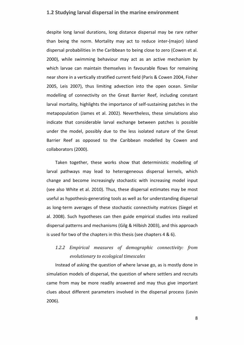
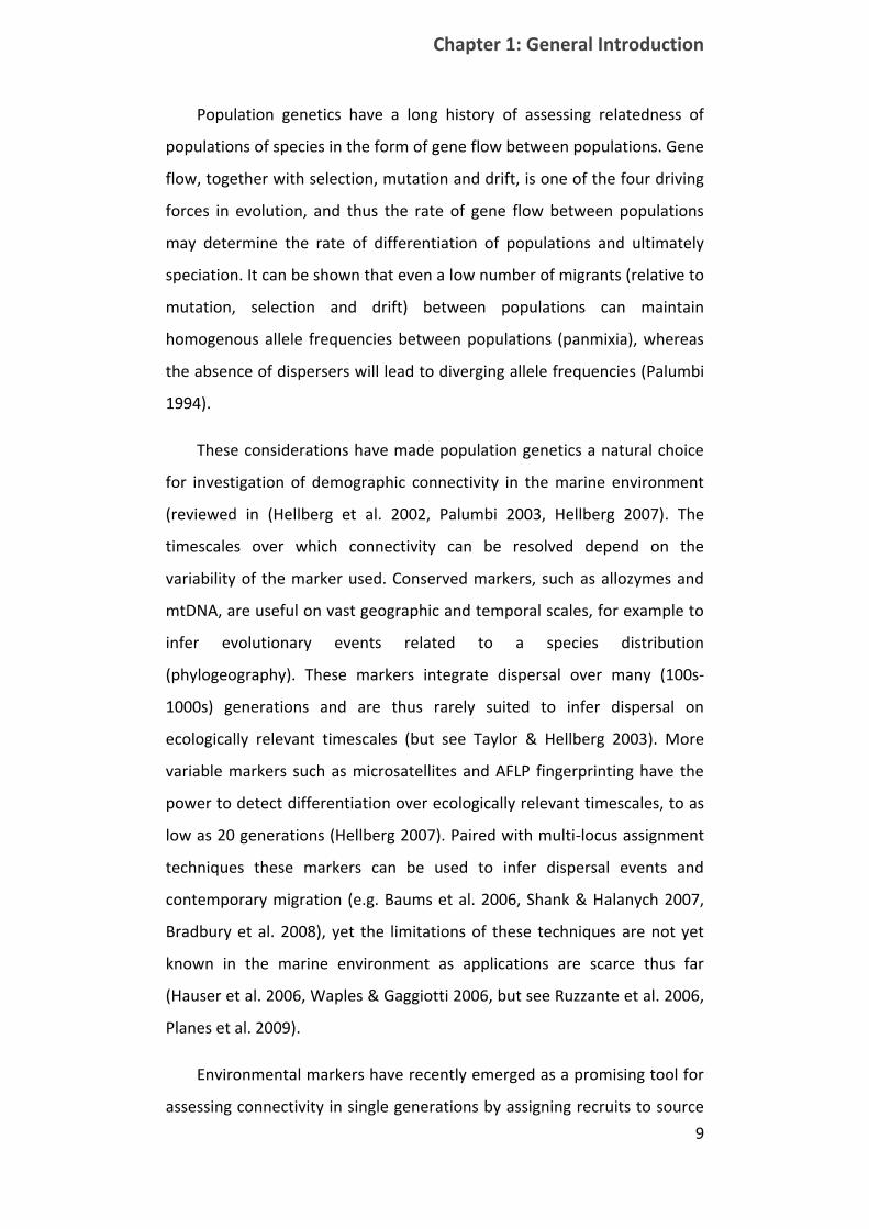
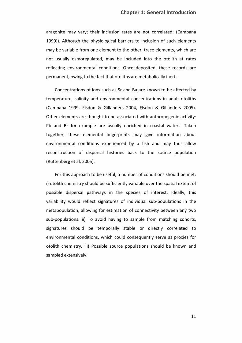
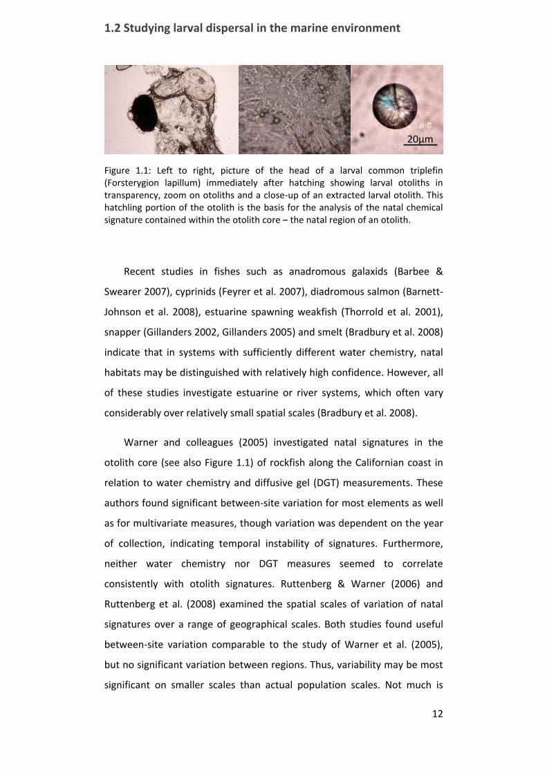
Figure 1.1: Left to right, picture of the head of a larval common triplefin (Forsterygion lapillum) immediately after hatching showing larval otoliths in transparency, zoom on otoliths and a close-up of an extracted larval otolith. This hatchling portion of the otolith is the basis for the analysis of the natal chemical signature contained within the otolith core – the natal region of an otolith.
Recent studies in fishes such as anadromous galaxids (Barbee &
Swearer 2007), cyprinids (Feyrer et al. 2007), diadromous salmon (Barnett-
Johnson et al. 2008), estuarine spawning weakfish (Thorrold et al. 2001),
snapper (Gillanders 2002, Gillanders 2005) and smelt (Bradbury et al. 2008)
indicate that in systems with sufficiently different water chemistry, natal
habitats may be distinguished with relatively high confidence. However, all
of these studies investigate estuarine or river systems, which often vary
considerably over relatively small spatial scales (Bradbury et al. 2008).
Warner and colleagues (2005) investigated natal signatures in the
otolith core (see also Figure 1.1) of rockfish along the Californian coast in
relation to water chemistry and diffusive gel (DGT) measurements. These
authors found significant between-site variation for most elements as well
as for multivariate measures, though variation was dependent on the year
of collection, indicating temporal instability of signatures. Furthermore,
neither water chemistry nor DGT measures seemed to correlate
consistently with otolith signatures. Ruttenberg & Warner (2006) and
Ruttenberg et al. (2008) examined the spatial scales of variation of natal
signatures over a range of geographical scales. Both studies found useful
between-site variation comparable to the study of Warner et al. (2005),
but no significant variation between regions. Thus, variability may be most
significant on smaller scales than actual population scales. Not much is
20μm
Chapter 1: General Introduction
13
known about the deterministic nature of these scales, and maternal effects
(Brophy et al. 2004, Chittaro et al. 2006) and small-scale changes in
concentration of elements in the water column (Campana 1999) may
influence otolith microchemistry on small scales and thus make signatures
too variable to be useful on larger scales. Thus, before this method can be
successfully applied to connectivity problems, the geographical resolution
and scale of variation of natal otolith signatures needs to be established.
This basic need provides the motivation for the first chapter of this thesis.
1.2.4 Profiles across otoliths: insights into dispersal histories
While otolith cores and the surrounding region may lead to insights
about natal origins of fish, profiles across otoliths of fish can provide
considerable information about their dispersal (Elsdon et al. 2008). Due to
the concentric growth of otoliths, time resolved measurements along the
growth axis may for instance provide information about the series of
environments a fish visited over the measured time (Elsdon et al. 2008),
and thereby give insights into ontogenetic shifts in habitat use (Miller et al.
2010), larval dispersal histories (Shima & Swearer 2009a, Shima & Swearer
2009b, Shima & Swearer 2010) and their demographic consequences as
well as adult migration patterns (Fowler et al. 2005). Studies of dispersal
pathways have further contributed to the definition of migratory
contingents within the concept of fish stocks (Secor & Piccoli 1996, Secor
1999). Contingents are intra-population groups of fish which display similar
migration histories, the existence of which can have important implications
for demographic processes and management (Secor 1999, Miller et al.
2010).
In order to reconstruct dispersal pathways from profiles across
otoliths, one needs to have an idea about the scales of variability in otolith
signatures in a system, and be able to connect a given signature to a
unique water mass. Again, this can be straightforward for diadromous fish,
but it may be more difficult in marine environments, where chemical
gradients are usually smoother and scales of variation are not immediately
1.3 Statistical methods for the analysis of otolith chemistry
14
obvious. The analysis of otolith profiles is ideally paired with studies of
variability within water masses (Elsdon et al. 2008). Often however,
hypotheses can be generated about the effects of different water masses
on otolith chemistry due to known relationships. In these situations, the
otolith profiles may be analysed in the light of such assumptions (Hamilton
et al. 2008, Shima & Swearer 2009a).
1.3 Statistical methods for the analysis of otolith chemistry
Whether it is isolated regions of the otolith or time resolved profiles,
the statistical analysis of otoliths is an important step in drawing robust
conclusions from this type of data. Data obtained from chemical analyses
of otoliths (usually using Laser ablation inductively coupled plasma mass
spectrometry) is noisy for a number of reasons, including environmental
variability (auto-correlated noise), measurement noise due to
contaminations (auto-correlated noise if contaminations are strong
enough) and measurement noise due to the method itself (white or
Gaussian noise). While the latter type of noise is usually not much of a
problem, the former two forms of noise can significantly alter the
inferences we make from otolith chemical measurements. Robust
processing and statistical analysis of such data is thus of foremost
importance.
Most recent analyses of otolith chemistry rely on either mixture
models or linear discriminant analysis for the characterization and
discrimination of water-masses from isolated scans of otolith chemistry
(White & Ruttenberg 2006). These models are intimately related, in that
the discriminant function analysis is a sub-class of a mixture model where a
single parameter is fixed. The joint probability density for a mixture model
can be written as:

Chapter 1: General Introduction
15
f(yj¼; µ) =
NY
i=1
KX
k=1
¼kf(yijµk)f(yj¼; µ) =
NY
i=1
KX
k=1
¼kf(yijµk)
(1.1)
The formalism in equation (1.1) states that the data y = (y1:::yi:::yN )y = (y1:::yi:::yN )
are distributed as a mixture density, with proportions ¼ = (¼1:::¼k:::¼K)¼ = (¼1:::¼k:::¼K)
originating from one of KK water-masses. f(yijµk)f(yijµk) is the conditional
density of water mass kk , parameterized by µkµk (with µ = (µ1:::µk:::µK)µ = (µ1:::µk:::µK))
evaluated at yiyi (the likelihood). One usually chooses a normal (or Gaussian)
density forff , although other distributions could be used. The proportions
of fish from water-mass or source kk is then ¼k = p(»i = k)¼k = p(»i = k), where »i»i assigns
individual ii to source kk. From this formulation it is possible to obtain the
posterior distribution of a fish belonging to one of KK water masses via
Bayes theorem:
p(»i = kjµ;y) =¼kf(yijµk)
PK
k0=1 ¼k0f(yijµk0)p(»i = kjµ;y) =
¼kf(yijµk)PK
k0=1 ¼k0f(yijµk0) (1.2)
The only difference between a mixture model and a discriminant
analysis is that for the latter the ¼k¼k are assumed to be known. Often,
homogeneity of variances is assumed as well (in linear discriminant analysis
for instance). If f (yjµ)f (yjµ) is known, say from a baseline sample, then assigning
fish to a water-mass or source can be directly done using equation (1.2) by
assigning to the source with the highest associated posterior probability. If
one treats the mixing proportions ¼k¼k as unknown, these need to be
estimated via maximum likelihood or Bayesian methods. With Bayesian
methods, ff may be treated as unknown as well and estimated from the
baseline sample at the same time (Munch & Clarke 2008, White et al.
2008).
Other methods can be used to assign fish to natal sources or different
water-masses. Thorrold et al. (1998) for instance used artificial neural
networks for classification of individual fish. While they found this
technique relatively successful, neural networks are prone to over-fitting
and this study remains the only study to have used this formalism in an
1.3 Statistical methods for the analysis of otolith chemistry
16
empirical context. Mercier et al. (in press) evaluated the performance of
linear discriminant analysis against machine learning techniques including
random forests and artificial neural networks. These authors found that
machine learning methods were more robust when the assumptions of
discriminant analysis were not met. A possible drawback of these methods
however is that they rely on a single baseline sample, and that baseline
characteristics are thus assumed to be known. A common limitation to all
of the above models is that the potential sources are assumed to be
known. This can be especially problematic in the marine environment
where it may not be possible to characterise all possible natal regions. This
limitation will be discussed in the following section.
The array of techniques used for the statistical analysis of otolith
profiles is larger still, reflecting the diversity of questions that can be
addressed with this type of data. The time-resolved nature of the data
necessitates special attention since measurements along the otolith profile
are usually not independent (Elsdon et al. 2008). Methods such as repeated
measures ANOVA, its mixed model analogue, and Multivariate ANOVA
(MANOVA) have been proposed to assess statistical significant differences
between sets of fish and their individual time-resolved signatures (Secor &
Piccoli 1996, Elsdon et al. 2008).
To answer more intricate questions, Shima and Swearer (2009a)
proposed a clustering framework based on time-series descriptors to
discover similarities in dispersal histories. Sandin et al. (2005) proposed a
likelihood framework to classify fish to ad hoc migratory classes based on
otolith profiles, and Hamilton et al. (2008) used an extension of this
framework to assign fish to retained or dispersed phenotypes. Finally,
Fablet et al. (2007) used a latent state modelling approach, comparing
mixture models with a hidden Markov model, to study habitat transitions
of European eels. This approach can be seen as a time-dependent
extension of the above mentioned mixture model (c.f. Chapter 4).
Chapter 1: General Introduction
17
1.3.1 Bayesian methods for otolith chemistry
Bayesian methods have dominated recent publications on mixture
modelling from both geochemical and genetic markers (Pella & Masuda
2001, Manel et al. 2005, Pella & Masuda 2006, Bolker et al. 2007, Munch &
Clarke 2008, White et al. 2008, Smith & Campana 2010). Of these, three
methods were specifically concerned with a Bayesian analysis of otolith
chemical signatures (Munch & Clarke 2008, White et al. 2008, Smith &
Campana 2010). While Smith & Campana’s model is designed to
accommodate genetic data also, the distinction between the type of data is
actually of little relevance to the model itself – the underlying sampling
distribution simply changes from a normal distribution for otolith data to a
multinomial one for genetic data and their likelihoods are multiplied for
each fish. The basic model setup is the same as in Bolker et al. (2007) for
genetic data, which in turn is adapted from Pella & Masuda (2001). Thus,
the distinction of methods for otoliths versus genetic data relies simply on
the sampling distribution used; the underlying models however are
equivalent.
Within these models (and other models discussed above) we may
distinguish conditional and unconditional models. Conditional models
receive their name because estimates of quantities of interest, such as
assignment probabilities and mixing proportions, are conditional on a
baseline sample and it’s estimated parameters. Thus, once these
characteristics are determined, they are considered to be fixed. This is the
setting of classical classification methods under which earlier mixture
models (Millar 1987) discriminant anlysis, neural networks, so-called
random forrests and related methods employed for classification based on
otolith chemistry can be grouped. Unconditional models on the other
hand will update the baseline in the light of the mixed sample at hand: the
parameters µµ are shared between the mixed sample and the baseline.
Koljonen et al. (2005) found that these methods can perform significantly
better than conditional methods, especially if baseline sizes are small
1.3 Statistical methods for the analysis of otolith chemistry
18
compared to the mixed stock. This is often the case in fisheries, rarely
however in ecological studies.
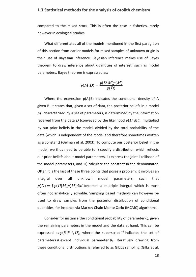
What differentiates all of the models mentioned in the first paragraph
of this section from earlier models for mixed samples of unknown origin is
their use of Bayesian inference. Bayesian inference makes use of Bayes
theorem to draw inference about quantities of interest, such as model
parameters. Bayes theorem is expressed as:
p(MjD) =p(DjM)p(M)
p(D)p(MjD) =
p(DjM)p(M)
p(D)
Where the expression p(A|B) indicates the conditional density of A
given B. It states that, given a set of data, the posterior beliefs in a model
MM , characterized by a set of parameters, is determined by the information
received from the data DD (conveyed by the likelihood p(DjM)p(DjM)), multiplied
by our prior beliefs in the model, divided by the total probability of the
data (which is independent of the model and therefore sometimes written
as a constant) (Gelman et al. 2003). To compute our posterior belief in the
model, we thus need to be able to i) specify a distribution which reflects
our prior beliefs about model parameters, ii) express the joint likelihood of
the model parameters, and iii) calculate the constant in the denominator.
Often it is the last of these three points that poses a problem: it involves an
integral over all unknown model parameters, such that
p(D) =Rp(DjM)p(M)dMp(D) =
Rp(DjM)p(M)dM becomes a multiple integral which is most
often not analytically solvable. Sampling based methods can however be
used to draw samples from the posterior distribution of conditional
quantities, for instance via Markov Chain Monte Carlo (MCMC) algorithms.
Consider for instance the conditional probability of parameter µiµi, given
the remaining parameters in the model and the data at hand. This can be
expressed as p(µijµ¡i;D)p(µijµ¡i;D), where the superscript ¡i¡i indicates the set of
parameters µµ except individual parameter µiµi . Iteratively drawing from
these conditional distributions is referred to as Gibbs sampling (Gilks et al.
Chapter 1: General Introduction
19
1996), a method which will asymptotically recovery the conditional
posterior distribution for each parameter. A multitude of other variants of
MCMC exist for situations in which we cannot explicitly write such
conditional distributions. Though different in terms of their efficiency, all of
these methods guarantee that samples will eventually be from the actual
posterior distribution. It is however not guaranteed that this happens in
any given amount of draws from the sampling scheme. It is therefore
important to either devise efficient algorithms which quickly converge to
the correct distribution, or run the sampler for a great number of iterations
(no method can however guarantee that this distribution has actually been
reached or fully explored by the resulting draws – which is usually not
much of a problem in practice when efficient schemes are used).
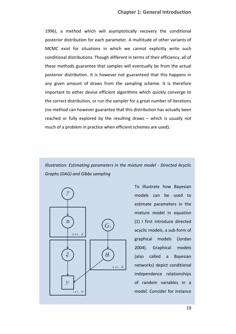
Illustration: Estimating parameters in the mixture model - Directed Acyclic
Graphs (DAG) and Gibbs sampling
To illustrate how Bayesian
models can be used to
estimate parameters in the
mixture model in equation
(1) I first introduce directed
acyclic models, a sub-form of
graphical models (Jordan
2004). Graphical models
(also called a Bayesian
networks) depict conditional
independence relationships
of random variables in a
model. Consider for instance

1.3 Statistical methods for the analysis of otolith chemistry
20
the mixture model considered in equation (1). The pictured DAG describes
the independence relationships within the model: A node is a random or
fixed variable in the graph, a descendent node is defined as the node to
which arrows point at any level in the in the graph, its parent nodes are
those from which arrows point to the descendent node. Most nodes will
thus be parents at one level and descendants of another level. In a DAG,
each descendent node is thus conditionally independent of nodes
preceding its parent node. Furthermore, plates (enclosing boxes in the
graph) show recurring structures, such as parameters being defined for
each individual ii or sourcekk.
Starting from the top of the graph, °° and G0G0 are the priors for the
mixing proportions ¼¼ and source specific parameters µ = (µ1:::µk:::µK)µ = (µ1:::µk:::µK)
respectively. ¼k¼k itself determines the probability p(»i = k)p(»i = k). However, given
the assignment »i = k»i = k and the source specific parameter vector µµ the
density for any yy does not depend on ¼¼. Similarly, given ¼¼ , » = (»1:::»:::»N)» = (»1:::»:::»N)
is independent of the prior °°.
This can be used when estimating parameters in the model: only the
direct parents and descendants of any node will carry direct information
regarding that node. One only needs to find conditional probabilities of
each parameter given directly related nodes instead of specifying the full
joint distribution over all parameters. Thus for the mixture model, we can
simply sample repeatedly (and in any order) from p(¼kj°; »)p(¼kj°; »), p(»ijyi;¼i)p(»ijyi;¼i),
p(»ijyi;¼)p(»ijyi;¼) and p(µkjy; G0)p(µkjy; G0). Often, some parameters can be integrated out
of the model (i.e. the posterior distribution for all sources can be obtained
analytically by integrating over µµ, which means that the Gibbs sampler only
involves two sampling steps, those for ¼¼ and »» (Casella & Robert 1996).
Chapter 1: General Introduction
21
Bayesian methods have a distinct advantage in that the breaking up of
the joint probability of a model into conditional relationships and the
sampling from resulting densities permits models of great complexity and
flexibility – although the need for complexity needs to be carefully
assessed for each model. Pella & Masuda (2001) provided the first tailored
Bayesian approach to mixture models for fisheries applications, which
explicitly uses the prior density to select for informative alleles within a set
of alleles. These authors also introduced the idea of directly modelling the
baseline data as a sample from an unknown distribution rather than a
collection of well-defined potential sources. Correctly estimating the effect
of this uncertainty about the baseline sample in the resulting posterior
distributions is a great advantage of the Bayesian method, and Koljonen et
al. (2005) found that these methods usually outperform non-Bayesian
methods. This is largely due to the unconditional (not to be confounded
with the conditional distributions from the Gibbs sampler) nature of the
model in which information is shared between the mixture and its baseline.
White et al. (2008) and Munch & Clarke (2008) proposed methods
tailored for otolith chemical data, but their analysis is rather different from
that of Pella & Masuda (2001). Munch & Clarke (2008) propose a
conditional model, in which fish are classified according to the posterior
predictive probability of each fish in the mixture given the baseline. The
posterior predictive distribution in Bayesian statistics is a distribution which
integrates over the posterior distribution of unknown parameters (given
the data) to predict the density of a new observation. This density can be
written as p(yijsi = k;x) =Rp(yijsi = k;µ)p(µjx)dµp(yijsi = k;x) =
Rp(yijsi = k;µ)p(µjx)dµ, where µµ are the
baseline parameters estimated from the baseline xx. Evaluating this integral
numerically leads to a so-called collapsed Gibbs sampler (a method that
also called Rao-Blackwellisation (Casella & Robert 1996)), which enhances
efficiency of the sampling procedure. Munch & Clarke’s method thus
incorporates uncertainty from finite baseline samples, but still has the
drawbacks of a necessarily known and fully sampled baseline.
1.4 Contributions of this thesis
22
White et al. (2008) propose a method which does not really fit one of
the above categories, it is more precisely a sub-form of both since it does
not explicitly model the baseline as an entity different to the mixed sample.
It is thus rather a clustering method which groups both the baseline and
the mixed sample into homogenous groups. These authors also propose
model selection to find the most likely number of sources in the mixture.
While this approach provides a promising way towards finding the number
of likely sources in a dataset, the underlying clustering model is limited in
that it does not use the baseline directly to classify fish of unknown origin,
but rather compares clusters obtained from the baseline and the mixed
sample.
For genetic mixtures, Pella & Masuda (2006) provide a way to directly
infer un-sampled baseline contributions. This method is based on a
Bayesian non-parametric prior formulation, using the Dirichlet Process
model. This model produces a marginal posterior distribution over the
number of sources in the baseline while assigning individuals to a set of
unknown underlying distributions. It thus has all the advantages of their
original model (Pella & Masuda 2001), without the constraint to have
sampled all contributing sources in the baseline. No comparable models
currently exist for geochemical data and chapter 3 of my thesis aims at
developing analogous methods which can be used with otolith chemistry.
Finally, no attempts have been made at a fully Bayesian analysis of the
time resolved signatures obtained from otolith profiles. The lack of such
methods for otolith data constitutes the motivation for chapter 5 of my
thesis.
1.4 Contributions of this thesis
My thesis develops a combination of empirical, statistical and
simulation approaches to analyse connectivity of marine fish
metapopulations. Novel statistical methods for otolith chemical data

Chapter 1: General Introduction
23
obtained from fish otoliths (Figure 1.1) allow me to infer connectivity
between local populations of common triplefin (Forsterygion lapillum,
Figure 1.2) in three marine reserves in Cook Strait. Comparing these
outcomes to newly developed simulation models of ocean currents
provides insights into the mechanisms of dispersal in this system.
Figure 1.2: Picture of an adult common triplefin (Forsterygion lapillum). © P.Neubauer
In chapter two I start by examining otolith signatures of F. lapillum
hatchlings from around Cook Strait, building an atlas (a baseline) of
variability in otolith signatures. I develop statistical methods which
examine the properties of this atlas and I discuss its value for connectivity
studies. Examining variability over a range of scales and environments
provides a complete picture of variability in otolith chemistry across a
variety of conditions and thereby contributes to our understanding about
the variability of these scales in marine environments. Additionally, this
chapter forms the basis for the remaining empirical work in this thesis.
My third chapter tackles the important question of finding natal origins
of fish when the geochemical atlas of potential natal sources is likely to be
incomplete. Dirichlet process mixture models provide the basis for a
solution to this limitation for geochemical studies: Fish recruits of unknown
origin are no longer just assigned to a natal source in a fixed atlas or

1.4 Contributions of this thesis
24
baseline, but are attributed to new sources if they are sufficiently different
from the existing baseline. I develop this approach for clustering and
classification with geochemical signatures and show its potential on the
weakfish dataset of Thorrold et al. (2001). These statistical advances open
new doors for the use of geochemical signatures in marine environments,
where a complete characterization of natal sources is often impossible.
For Chapter 4 I collected F. lapillum recruits from three marine
reserves in Cook Strait in order to explore whether connections between
different regions and their reserves are evident. I employ the statistical
methods developed in chapter 3 to find possible natal sources of these
settlers and develop a simulation model which provides a potential
mechanistic understanding of the dispersal patterns evidenced by otolith
chemistry. To simulate dispersal, I outline a new refining grid model of
hydrodynamics in Cook Strait, which provides a state-of-the-art tool to look
at potential dispersal pathways in Cook Strait. A qualitative comparison of
dispersal of passive particles in the model and empirical findings offers
important scrutiny and validation of empirical results.
The fifth chapter builds on existing models to provide a general and
flexible approach to modelling fish dispersal pathways from time series of
otolith chemistry obtained by sampling the otolith chemistry longitudinally
(along the growth axis). I illustrate how this general method can be applied
in a variety of situations pertaining to a number of ecological questions
often studied with this type of data. Additionally, I demonstrate how this
approach provides a basis for model selection which can aid in deciding
between competing hypotheses and to find appropriate models for a given
dataset. The strengths and limitations of models based on this underlying
framework are then illustrated with a set of simulation studies and a
dataset of Chinook salmon (Miller et al. 2010), for which I investigate the
size distribution at freshwater emigration based on otolith chemistry.

Chapter 1: General Introduction
25
Figure 1.3: A Coastal boundary layer often forms from terrestrial runoff, visible in this NASA satellite image, motivating the model formulation in chapter 4.
The sixth and final data chapter applies the modelling approach
developed in chapter five to chemical profiles across otoliths of the recruits
collected for chapter 4 in order to get a better understanding of the
mechanisms which underlie dispersal of F. lapillum in Cook Strait. To this
end I develop a model which distinguishes between inshore and offshore
water masses (Figure 1.3) in Cook Strait which provides insights into the
dispersal traits of successful settlers in these populations. Idealized
simulations with the adaptive grid ocean model developed in chapter 4
illustrate the benefits of these traits for maintaining metapopulation
connectivity in the highly advective waters of Cook Strait.
I conclude my thesis by discussing the implications of my
methodological and empirical findings in the context of marine
metapopulations and the study of their connectivity and spatial structure.

26

* A version of this chapter has been published in Marine Ecology Progress
Series Vol. 415: 263-274, 2010 27
Chapter 2:
2. Scale-dependent variability in hatchling otolith
chemistry: implications for studies of
population *
2.1 Introduction
Patterns of connectivity among spatially discrete local populations
have important consequences for the dynamics and behaviour of local
populations and the larger metapopulation (Caley et al. 1996, Cowen et al.
2000). Nonetheless, our understanding of patterns of connectivity in
coastal marine systems remains limited. Connectivity in many marine
metapopulations is generally facilitated by dispersal of larvae. While larval
durations can last weeks to months for some species, recent evidence
suggests that long distance dispersal may be a relatively rare occurrence
(Cowen et al. 2006), and self-recruitment could be important in some
populations (see Swearer et al. 2002 for a review). Obtaining more
complete knowledge of dispersal patterns in marine metapopulations is of
critical importance if we hope to understand some of the key drivers of
marine population dynamics.
In teleost fishes, otoliths (fish ‘ear stones’) are increasingly used to
address dispersal questions (e.g. Campana & Thorrold 2001, Thorrold et al.
2002, Elsdon & Gillanders 2003, Shima & Swearer 2009a). Otoliths are
2.1 Introduction
28
known to act as environmental recorders during a fish’s life (Campana &
Thorrold 2001): trace elements in the developmental environment are
incorporated into growing otoliths and may reflect local environmental
conditions (Campana 1999). Otoliths are metabolically inert, such that once
deposited, trace element signatures form a permanent record. Trace
element signatures can facilitate reconstruction of dispersal histories (e.g.
Elsdon & Gillanders 2003, Hamilton et al. 2008, Shima & Swearer 2009a)
and classification of individuals to putative natal source populations (e.g.
Thorrold et al. 2002, Gillanders 2005, Ruttenberg et al. 2005).
Brophy et al. (2004) documented evidence for a peak of Mn in cores
(the natal region) of otoliths in two species of fish, and Ruttenberg et al.
(2005) extended these findings to six other species. The distinct manganese
peak may thus serve as a marker of the core in otoliths sampled from older
individuals, which may in turn act as a marker of natal conditions
(Ruttenberg et al. 2005, Barbee & Swearer 2007, Ruttenberg et al. 2008).
Comparing trace element signatures from the otolith cores of settlers
and/or recruits to an ‘atlas’ of trace element signatures (e.g., constructed
from the otoliths of hatchlings, collected from known locations) could
facilitate the assignment of settlers and/or recruits to natal populations of
origin. The utility of this approach relies upon sufficient spatial variation in
natal (core) otolith chemistry over the scale of this ‘atlas’ to enable settlers
of unknown origin to be assigned to putative natal source populations with
a high level of confidence.
Little is known about scales of variability of hatchling otolith trace
element signatures in coastal environments. To date, most studies that
have employed this approach in marine environments have focused on
island chains (Warner et al. 2005, Ruttenberg & Warner 2006, Ruttenberg
et al. 2008) evidencing significant between-site variation within islands for
trace element signatures. At larger spatial scales, among-site differences in
signatures may overlap with those of other regions, and the discrimination
of sites on these scales may prove problematic (Ruttenberg & Warner
Chapter 2. Scale-dependent variability in hatchling otolith chemistry
29
2006, Ruttenberg et al. 2008). In addition, natal signatures may be
influenced by maternal or physiological effects (Campana 1999, Thorrold et
al. 2006, S. Swearer unpublished data), such that clutches from different
mothers within sites may differ markedly in signatures, and this source of
variation could mask contributions from environmental signals to limit
inferences relating to natal origins. Thus, before this overall approach can
be successfully applied to address many questions of population
connectivity, the geographical resolution and population specificity of
hatchling otolith signatures needs to be established (Ruttenberg et al.
2008).
Additionally, statistical approaches to explore and utilize patterns in
hatchling otoliths have been largely limited to statistical testing and linear
discriminant analysis (LDA). Though LDA is generally practical for the
assignment of recruits to possible sources (White & Ruttenberg 2006), it
may be limiting when the atlas is incomplete (Munch & Clarke 2008, White
et al. 2008). Alternatives have been suggested (Munch & Clarke 2008) but
their utility has not been empirically evaluated (but see White et al. 2008
for a related treatment of this problem). Furthermore, the proportion of
correctly assigned individuals in a discrimination problem will diminish with
an increasing number of classes (Smouse et al. 1982, Gillanders 2005,
Barbee & Swearer 2007). This has prompted some authors to consider
spatially aggregating sites to counteract this effect (e.g. Gillanders 2002).
While spatial aggregation of sites can be straightforward in simple
geographical contexts (e.g., linear coastlines), the same is not necessarily
true for more complex coastal geometries. In such contexts, no methods
currently exist to find optimal groupings and therefore optimize the
usefulness of hatchling otoliths as proxies for natal origins of fish.
The purpose of this chapter is twofold: (1) I explore patterns of
variation in hatchling otolith signatures using a hierarchical (i.e., spatially
nested) sampling design around Cook Strait, New Zealand, spanning a wide
range of environmental conditions in the region. This approach enables me
2.2 Methods
30
to evaluate sources of variation and infer plausible spatial scales of
resolution that may be achievable using hatchling otolith microchemistry
for my study system and species. (2) I describe and evaluate two
approaches that may be used to improve the resolution and strength of
inferences derived from trace element signatures. First, I employ a
simulated annealing algorithm (e.g. Dupanloup et al. 2002) which
statistically optimizes the spatial groupings of sites in order to increase the
probability of correctly assigning individuals of unknown origin to their
natal location. Second, I trial an ‘exclusion test’ approach (Cornuet et al.
1999, Munch & Clarke 2008, Standish et al. 2008), which has been
suggested for situations where not all possible source locations can be
referenced within the natal atlas. I test the utility of this approach for my
data by performing exclusion tests on otolith signatures of known origin to
identify the spatial scales at which this approach can provide the most
robust assignment of larval origins.
2.2 Methods
2.2.1 Study Species & Sampling
My focal species for this study is the common triplefin Forsterygion
lapillum, a small reef fish that is ubiquitous on relatively sheltered rocky
reefs and tide pools around New Zealand, to a depth of ~10m (Clements
2003). Adults are strongly site attached, with a home range limited to a few
square meters (Clements 2003, Wellenreuther et al. 2007). Females lay
benthic eggs almost year-round within the study area (Wellenreuther &
Clements 2007, P. Neubauer, pers. obs.), typically on the underside of
smooth cobbles, and nests are guarded by territorial males until hatching.
Larvae hatch after ~10 days (P. Neubauer, unpublished data) and settle
back to subtidal reefs in the region after a ~52 day pelagic larval duration
(PLD) (Shima and Swearer 2009). I employed a hierarchical sampling design
that included locations on both sides of the Cook Strait (the divide between
the North and South Islands of New Zealand, Figure 2.1). The spatial extent
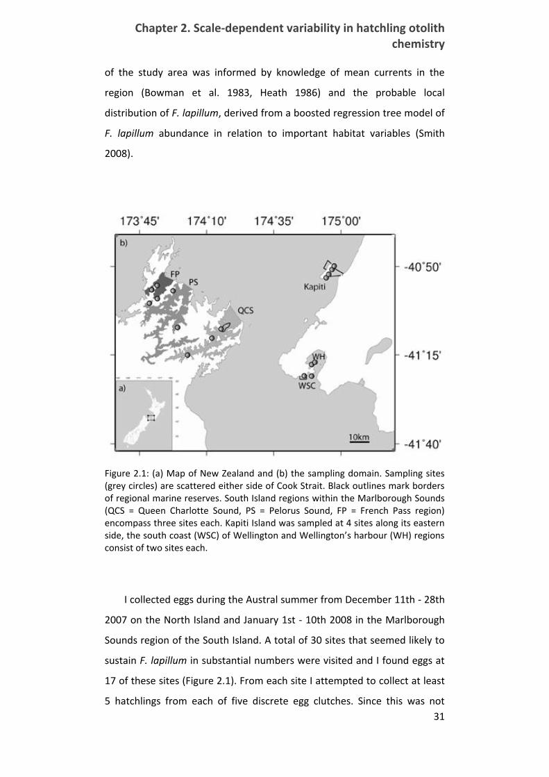
Chapter 2. Scale-dependent variability in hatchling otolith chemistry
31
of the study area was informed by knowledge of mean currents in the
region (Bowman et al. 1983, Heath 1986) and the probable local
distribution of F. lapillum, derived from a boosted regression tree model of
F. lapillum abundance in relation to important habitat variables (Smith
2008).
Figure 2.1: (a) Map of New Zealand and (b) the sampling domain. Sampling sites (grey circles) are scattered either side of Cook Strait. Black outlines mark borders of regional marine reserves. South Island regions within the Marlborough Sounds (QCS = Queen Charlotte Sound, PS = Pelorus Sound, FP = French Pass region) encompass three sites each. Kapiti Island was sampled at 4 sites along its eastern side, the south coast (WSC) of Wellington and Wellington’s harbour (WH) regions consist of two sites each.
I collected eggs during the Austral summer from December 11th - 28th
2007 on the North Island and January 1st - 10th 2008 in the Marlborough
Sounds region of the South Island. A total of 30 sites that seemed likely to
sustain F. lapillum in substantial numbers were visited and I found eggs at
17 of these sites (Figure 2.1). From each site I attempted to collect at least
5 hatchlings from each of five discrete egg clutches. Since this was not
2.2 Methods
32
always possible (due to the scarcity of clutches or the failure of some
clutches to hatch), some of the sites in this study are represented by 3-4
clutches but 6-8 hatchlings per clutch to have comparable number of
hatchlings from each site.
Clutches were collected using SCUBA or snorkelling in <3m depth.
Cobbles or rocks containing late-stage eggs (indicated by embryos with
visible eye spots) were collected by hand and placed in a sterile plastic bag
along with ~ 2L of water from the location of collection. On shore, the
contents of bags were emptied into clean PVC buckets with lids, such that
individual clutches were submerged and maintained in ambient water from
the natal site of collection. All but two clutches (both from one site at
Kapiti Island) hatched within 30min after collection. The remaining two
clutches were kept in the lab (in sea water from the site of collection,
supplemented with bubbled air) for 36 and 48h, respectively. These
clutches were excluded from later statistical analysis because signatures
were substantially different from clutches that hatched immediately at this
site, indicating possible handling effects. After hatching, all larvae were
transferred into 0.2ml Eppendorf tubes containing 95% analytical grade
ethanol, and transported to the lab for otolith extraction and analysis.
2.2.2 Otolith extraction, preparation and analysis
Hatchling otoliths were extracted individually from fish, in a
randomized order, under a laminar flow fume hood. To further minimise
the risk of contamination (which could confound trace element signatures
measured within otoliths), all material used during extraction and
preparation of the otoliths was acid rinsed for 24h in 6N HCL, then rinsed
three times in Millipore 18.2 MΩ water prior to use. Individual hatchlings
(i.e., larvae) were placed in a droplet of Millipore water on a clean slide and
a sagittal otolith was extracted from each larva. Otoliths were subjected to
cleaning and rinsing baths as in Barbee & Swearer (2007) before being
embedded in resin on a gridded slide. A Varian Laser Ablation Inductively
Coupled Plasma Mass Spectrometer (LA-ICPMS) at the University of
Chapter 2. Scale-dependent variability in hatchling otolith chemistry
33
Melbourne was used to analyse eleven trace elements contained within
the hatchling otoliths (7Li, 11B, 24Mg, 31P, 34S, 55Mn, 63Cu, 66Zn, 88Sr, 138Ba,
208Pb). Otoliths were ablated vertically in a deepening pit resulting in a
series of readings from the surface of the otolith through the core. For
further details of the extraction-, preparation- and analytical methods, see
Barbee & Swearer (2007).
All data were post-processed with calculations being identical to those
used in Barbee & Swearer (2007). Time series resulting from this processing
were inspected visually to check for signs of surface contamination.
Specifically, I inspected the first and last readings corresponding to the
otolith surface, looking for elevated peaks in elements such as Zn and Pb,
which are prone to contamination. 10 scans to either side of the
manganese peak (interpreted as the otolith primordium) were averaged to
obtain the natal trace element signatures for subsequent statistical
analyses.
2.2.3 Statistical analysis
2.2.3.1 Descriptive statistics, significance testing and discrimination
I employed a nested model to explore patterns and sources of
variation in trace element signatures across all levels of the hierarchical
sampling design. ‘Clutches’ (Level 1 – random effect) were nested within
‘sites’ (Level 2 – random effect), which were in turn nested within the
different (a priori defined) ‘regions’ (Level 3 – fixed effect) distributed
across both main ‘islands’ (Level 4 – fixed effect) of New Zealand,
separated by the Cook Strait. Note that by making such arbitrary groupings,
I make implicit assumptions about processes that govern geographical
patterns in otolith chemistry - i.e. I assume that all sites within a region are
influenced by a region specific generative process. I further assume that
the regions represented here cover all possible spawning locations
(motivating the fixed effect for this level). I address this issue in more detail
below. I performed non-metric multidimensional scaling (MDS) to visually

2.2 Methods
34
inspect similarities at different levels of the hierarchy (e.g. sites in the
sampling domain, and clutches that hatched at different times - see
previous section ‘Study Species & Sampling’).
To test significance at different levels of the sampling design I opted for
permutation based multivariate analysis of variance (Anderson 2001). All
data were standardized to unit variance. Standardized data were permuted
within levels of the nested hierarchy so as to keep the higher level fixed
while permuting the next lower level to avoid testing against variability at
other levels (Anderson 2001). All levels were tested with 9999
permutations. Significance testing was conducted using PRIMER software
with PERMANOVA add-on (Anderson 2001, Anderson et al. 2008). As this
was a mixed model, components of variation were calculated as sums-of-
squares divided by degrees of freedom for fixed effects and as variance
components derived from expected mean squares for random effects
(Anderson et al. 2008).
To facilitate comparisons with earlier studies, I used linear discriminant
analysis (LDA) of log-transformed data to discriminate amongst classes in
levels of the sampling hierarchy. Linear discriminant analysis (LDA) has
been widely used to classify and assign hatchling otoliths to potential
source populations, though other classifiers are preferred in certain
situations (Mercier et al. in press). The usefulness of the hatchling otolith
'atlas' is ultimately measured by its ability to successfully discriminate
amongst putative source populations. I chose to evaluate the performance
of this method based on the overall classification success of hatchling
otoliths (with known geographic origins), using “leave-one-out” cross
validation as an indicator of performance of the technique at different
levels of the sampling hierarchy. Since this measure represents an estimate
from the sample at hand, I used 1000 parametric bootstrap samples
(drawing from a multivariate normal distribution with mean and covariance
matrix of log-transformed data) for each source to calculate confidence
limits of cross validation results as 2.5% and 97.5% quantiles of the
Chapter 2. Scale-dependent variability in hatchling otolith chemistry
35
bootstrap distribution. I also calculated the relative contribution of each
element to class separation by calculating their contribution to the F ratio
(the ratio of between class variability to within class variability).
To visually illustrate the signal to noise ratio of levels of the hierarchy, I
plotted the mean Mahalanobis distance at each level, which is the
Euclidian distance between group means (the 'signal') weighted by intra-
group variance (the 'noise'), against number of groups and expected
assignment success (Smouse et al. 1982, White & Ruttenberg 2006). All
analyses in this and the following sections were conducted using the
statistical computing language R (R Development Core Team 2007).
2.2.3.2 Optimal grouping of sites by simulated annealing
I initially imposed a hierarchical spatial structure on the sampling
programme (e.g., defining discrete regions within islands, etc.), but this
structure might not represent natural underlying scales of variability in
trace element signatures. To identify optimal, non-a priori groupings of
sites that might improve the allocation success of unknown signatures (and
thus, improve the power of the approach), I used a simulated annealing
(SA) algorithm. SA is a general optimization heuristic that can locate global
optima in combinatorial problems. The procedure used here essentially
follows a simple SA algorithm (e.g. Burkard & Rendl 1984). At each iteration
of the algorithm, a spatial configuration, which conforms to constraints in a
contiguity matrix, is proposed (only adjacent sites can be grouped).
Problem related constraints were added where needed (see also
Dupanloup et al. 2002 for a related simulated annealing algorithm in
genetics).
2.2 Methods
36
The procedure can be summarized as follows:
1. Propose any starting configuration, such as the a priori groupings
2. Randomly choose to either merge two adjacent sites/clusters of
sites or to remove a site from a cluster. This involves a Bernoulli
trial (merge/split) with probability 0.5 followed by two multinomial
trials T = fi; jgT = fi; jg with probability 1NT
1NT
(sites or clusters II and JJ to
merge or site JJ to remove from cluster II , where II , JJ are the
outcomes of trials ii and jj respectively), where NTNT is the number of
possible choices in each trial. Note that NTNT for trial JJ is dependent
on the outcome of trial II.
3. Calculate the value of the cost function EE. In this case this is the
expected assignment accuracy for the new configuration (Smouse
et al. 1982). Accept the new grouping if Es2S > max(E1:s¡1)Es2S > max(E1:s¡1), else
accept with probability proportional to the difference of
Es ¡Es¡1 = ¢EEs ¡Es¡1 = ¢E , namely exp(¢E¿)exp(¢E
¿) .
4. Return to step 2 for SS iterations
The variable ¿¿ is called the temperature with analogy to related
physical problems. It is decreased (logarithmically in this case) with the
number of iterations, such that, at the initiation of the procedure,
suboptimal configurations are accepted with high probability. In later
iterations, suboptimal configurations become increasingly unlikely. This
progressive decrease in the acceptance of suboptimal configurations
enables the algorithm to overcome local optima and identify a global
optimum. A more conventional clustering approach would yield a single
(but potentially sub-optimal) cluster configuration; the SA approach
facilitates a more thorough exploration of all possible configurations to
increase the likelihood of arriving at a globally optimal solution.
I ran the algorithm with three different additional constraints: (1) any
spatial configuration of sites was allowed except re-grouping across islands
Chapter 2. Scale-dependent variability in hatchling otolith chemistry
37
– this restriction was always applied since I felt that the reasonable
discriminatory power at this scale (see results) made regroupings across
islands unnecessary and counter-productive - (2) the optimal solution must
differentiate at least four groups (SA4) and (3) the optimal solution was
biased in favour of many small groupings (SA MS). For this last constraint
the cost function was modified by multiplying the expected classification
success by the number of groupings (favours many groups) and then
dividing by the size of groups (favours small groups). Note that by
introducing a constant in this fraction, the cost function can be arbitrarily
modified to give selection criteria that favour resolution or overall
classification success. Post-hoc permutational multivariate analysis of
variance was performed on groupings obtained from the different
constraint scenarios.
2.2.3.3 Exclusion test
For some applications and research questions, it may not be possible or
necessary to construct a definitive atlas of natal signatures (e.g. Elsdon et
al. 2008). In such instances, it may still be useful to differentiate between
individuals that likely originated from a particular location (e.g., a natal
source population within a marine reserve) versus all other locations. To
test whether such questions can be addressed with hatchling otoliths, I
applied an ‘exclusion test’ framework to a subset of the data. Here, the
focus is on sub-groups within the sampling area, and I applied a statistical
approach to evaluate the probability that individuals of unknown origin do
not belong to a grouping of interest (Cornuet et al. 1999, Barbee & Swearer
2007, Munch & Clarke 2008, Standish et al. 2008). Using log-transformed
trace element signatures from hatchling otoliths, I calculated Mahalanobis
distances from the centroid of the focal group to samples known to
originate from all other sites (i.e., individuals with natal origins other than
the focal population). The distribution of squared Mahalanobis distances
from a multivariate normal distribution follows a χ² distribution with p
degrees of freedom, where p is the dimension of the data. This
2.3 Results
38
distribution can thus be used as the null distribution and one can look up
the critical value (α=0.05 for instance) for belonging to a focal group/site
(represented by this distribution) in a standard χ² table. Samples whose
squared Mahalanobis distance to the centroid of the focal group/site is
above this critical value can then be considered to have originated from a
source outside the focal population (Munch & Clarke 2008).
To illustrate the potential utility of this approach, I applied this
exclusion test to a subset of my data that included individual sites and
groups of sites within Pelorus Sound and Kapiti Island (two regions of high
and low separation, respectively). Additionally, I investigated exclusion
potential from two marine reserves in my dataset: Long Island Marine
Reserve in the Marlborough Sounds and Island Bay (Taputearanga Marine
Reserve) on the Wellington south coast. Since these results may be an
artefact of sampling (i.e., unsampled sites may have similar signatures to
sampled ones), I repeated these tests for one case (Pelorus Sound), each
time dropping 2, 5 or 10 randomly selected sites from the test. This
approach enabled me to evaluate the power of the exclusion potential for
this site or subset of sites for a given sampling effort.
2.3 Results
2.3.1 Descriptive statistics, significance testing and discrimination
Table 2.1 gives statistics relevant to chemical analyses, detection limits,
as well as precision estimates. Only Li and Pb were routinely below
detection limit, and neither element contributed to differences between
sites (Table 2.2). I identified significant variation among clutches within
sites (P = 0.0001), among sites within a priori defined regions (P<0.0001)
and between islands (P=0.0002) (Table 2.2a). The a priori regions within
islands were not significantly different (P=0.43), and their difference
explained 0.2% of the overall variance in the dataset. Small-scale
differences in trace element signatures explained the largest portion of the
Chapter 2. Scale-dependent variability in hatchling otolith chemistry
39
variance, with sites accounting for 7.9%, whereas clutch differences within
these locations explained 11.8%. A total of 72.8 % of the total variance in
the between signatures remained unexplained by the terms in the model
(i.e., variation among eggs within clutches).
Jackknife cross validation on LDA with equal prior probabilities for all
classes indicated that 76.2% (CI 74.4%-78.9%) of hatchlings could be
correctly assigned to their natal island despite overlap of distributions
(Table 2.2a, Figure 2.2a). A total of 34.9% (CI 33.4%-43.8%) of hatchlings
were correctly assigned to the pre-defined regions (Table 2.2a), and the
separation between these regional groupings was relatively poor (Figure
2.2b, c). Sites of natal origin were correctly assigned for only 32.5% (CI
29.7%-33.2%) of hatchlings (Table 2.2a) in the total dataset, but showed
the highest signal to noise ratio (Figure 2.3) of all levels in the hierarchy.
Additionally, sites from different regions were often more similar than sites
within regions (Figure 2.4); i.e., sites often overlapped in their distributions.
When restricting the domain to just a single region, I could correctly assign
79.8% (CI 73.1%-86.0%) of hatchlings to their natal site of origin within
Pelorus Sound (Table 2.2b, Figure 2.2d), and 56.4% (CI 50.1%-63.5%) within
Kapiti (Table 2.2b), even though trace element signatures for the sites
within Kapiti were not significantly different.
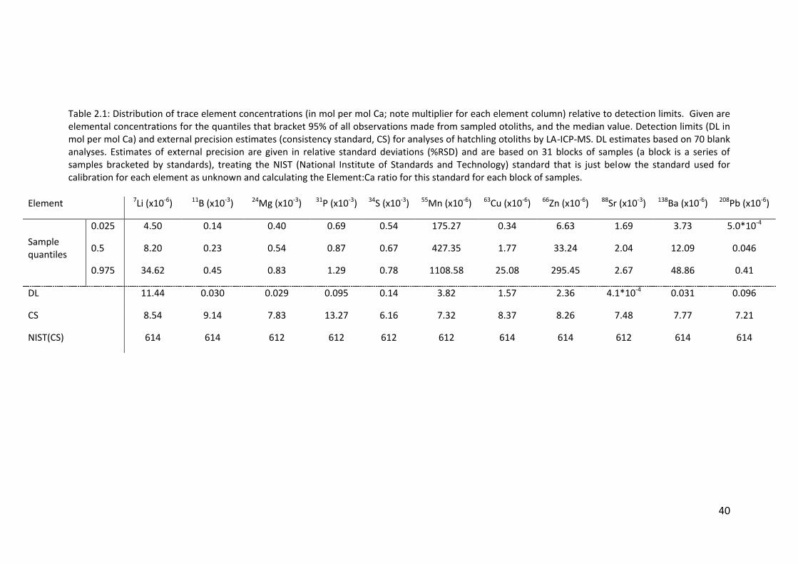
40
Table 2.1: Distribution of trace element concentrations (in mol per mol Ca; note multiplier for each element column) relative to detection limits. Given are elemental concentrations for the quantiles that bracket 95% of all observations made from sampled otoliths, and the median value. Detection limits (DL in mol per mol Ca) and external precision estimates (consistency standard, CS) for analyses of hatchling otoliths by LA-ICP-MS. DL estimates based on 70 blank analyses. Estimates of external precision are given in relative standard deviations (%RSD) and are based on 31 blocks of samples (a block is a series of samples bracketed by standards), treating the NIST (National Institute of Standards and Technology) standard that is just below the standard used for calibration for each element as unknown and calculating the Element:Ca ratio for this standard for each block of samples.
Element 7Li (x10-6) 11B (x10-3) 24Mg (x10-3) 31P (x10-3) 34S (x10-3) 55Mn (x10-6) 63Cu (x10-6) 66Zn (x10-6) 88Sr (x10-3) 138Ba (x10-6) 208Pb (x10-6)
Sample quantiles
0.025
0.5
0.975
4.50
8.20
34.62
0.14
0.23
0.45
0.40
0.54
0.83
0.69
0.87
1.29
0.54
0.67
0.78
175.27
427.35
1108.58
0.34
1.77
25.08
6.63
33.24
295.45
1.69
2.04
2.67
3.73
12.09
48.86
5.0*10-4
0.046
0.41
DL 11.44 0.030 0.029 0.095 0.14 3.82 1.57 2.36 4.1*10-4 0.031 0.096
CS 8.54 9.14 7.83 13.27 6.16 7.32 8.37 8.26 7.48 7.77 7.21
NIST(CS) 614 614 612 612 612 612 614 614 612 614 614
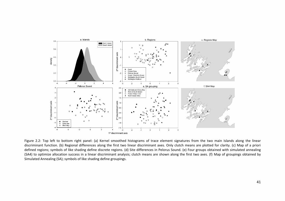
41
Figure 2.2: Top left to bottom right panel: (a) Kernel smoothed histograms of trace element signatures from the two main Islands along the linear discriminant function. (b) Regional differences along the first two linear discriminant axes. Only clutch means are plotted for clarity. (c) Map of a priori defined regions; symbols of like shading define discrete regions. (d) Site differences in Pelorus Sound. (e) Four groups obtained with simulated annealing (SA4) to optimize allocation success in a linear discriminant analysis; clutch means are shown along the first two axes. (f) Map of groupings obtained by Simulated Annealing (SA); symbols of like shading define groupings.
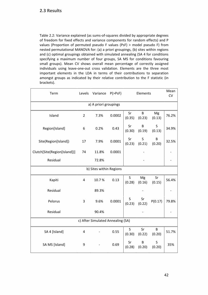
2.3 Results
42
Table 2.2: Variance explained (as sums-of-squares divided by appropriate degrees of freedom for fixed effects and variance components for random effects) and P values (Proportion of permuted pseudo F values (PsF) > model pseudo F) from nested permutational MANOVA for: (a) a priori groupings, (b) sites within regions and (c) optimal groupings obtained with simulated annealing (SA 4 for conditions specifying a maximum number of four groups, SA MS for conditions favouring small groups). Mean CV shows overall mean percentage of correctly assigned individuals using leave-one-out cross validation. Elements are the three most important elements in the LDA in terms of their contributions to separation amongst groups as indicated by their relative contribution to the F statistic (in brackets).
Term Levels Variance P(>PsF) Elements Mean
CV
a) A priori groupings
Island 2 7.3% 0.0002 Sr
(0.35) B
(0.23) Mg
(0.13) 76.2%
Region[Island] 6 0.2% 0.43 Sr
(0.30) B
(0.19) S
(0.13) 34.9%
Site(Region[Island]) 17 7.9% 0.0001 Sr
(0.23) S
(0.21) B
(0.20) 32.5%
Clutch[Site(Region[Island])] 74 11.8% 0.0001 - -
Residual 72.8% - -
b) Sites within Regions
Kapiti 4 10.7 % 0.13 S
(0.28) Mg
(0.16) Sr
(0.15) 56.4%
Residual 89.3% - -
Pelorus 3 9.6% 0.0001 S
(0.23) Sr
(0.22) P(0.17) 79.8%
Residual 90.4% - -
c) After Simulated Annealing (SA)
SA 4 [Island] 4 - 0.55 S
(0.30) Sr
(0.22) B
(0.20) 51.7%
SA MS [Island] 9 - 0.69 Sr
(0.28) B
(0.20) S
(0.20) 35%
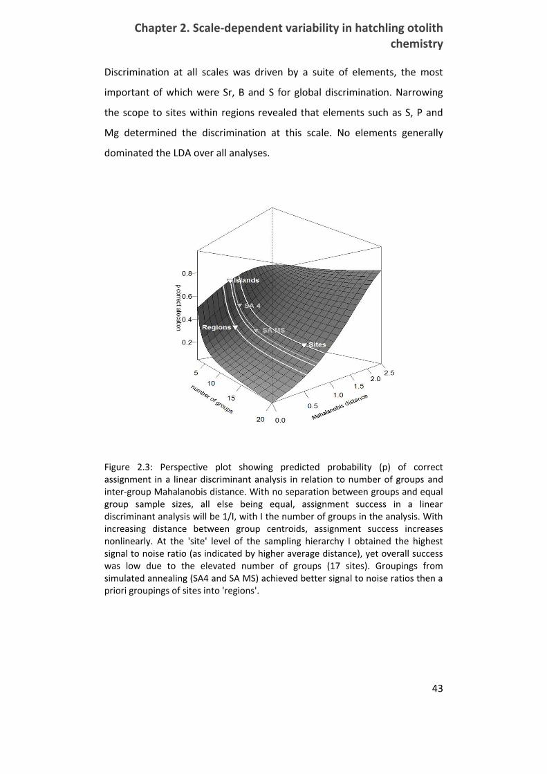
Chapter 2. Scale-dependent variability in hatchling otolith chemistry
43
Discrimination at all scales was driven by a suite of elements, the most
important of which were Sr, B and S for global discrimination. Narrowing
the scope to sites within regions revealed that elements such as S, P and
Mg determined the discrimination at this scale. No elements generally
dominated the LDA over all analyses.
Figure 2.3: Perspective plot showing predicted probability (p) of correct assignment in a linear discriminant analysis in relation to number of groups and inter-group Mahalanobis distance. With no separation between groups and equal group sample sizes, all else being equal, assignment success in a linear discriminant analysis will be 1/I, with I the number of groups in the analysis. With increasing distance between group centroids, assignment success increases nonlinearly. At the 'site' level of the sampling hierarchy I obtained the highest signal to noise ratio (as indicated by higher average distance), yet overall success was low due to the elevated number of groups (17 sites). Groupings from simulated annealing (SA4 and SA MS) achieved better signal to noise ratios then a priori groupings of sites into 'regions'.
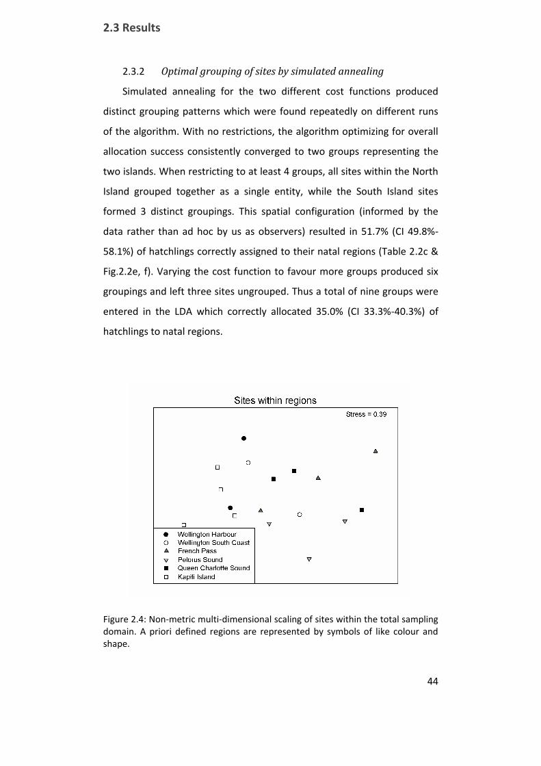
2.3 Results
44
2.3.2 Optimal grouping of sites by simulated annealing
Simulated annealing for the two different cost functions produced
distinct grouping patterns which were found repeatedly on different runs
of the algorithm. With no restrictions, the algorithm optimizing for overall
allocation success consistently converged to two groups representing the
two islands. When restricting to at least 4 groups, all sites within the North
Island grouped together as a single entity, while the South Island sites
formed 3 distinct groupings. This spatial configuration (informed by the
data rather than ad hoc by us as observers) resulted in 51.7% (CI 49.8%-
58.1%) of hatchlings correctly assigned to their natal regions (Table 2.2c &
Fig.2.2e, f). Varying the cost function to favour more groups produced six
groupings and left three sites ungrouped. Thus a total of nine groups were
entered in the LDA which correctly allocated 35.0% (CI 33.3%-40.3%) of
hatchlings to natal regions.
Figure 2.4: Non-metric multi-dimensional scaling of sites within the total sampling domain. A priori defined regions are represented by symbols of like colour and shape.
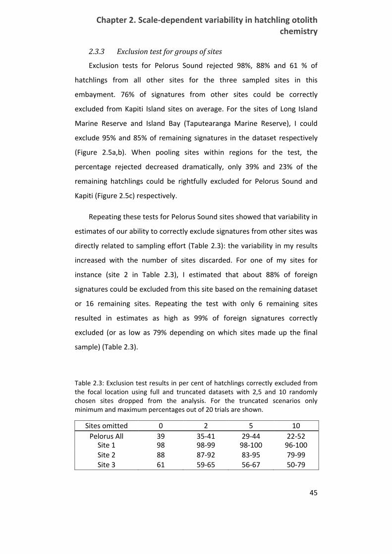
Chapter 2. Scale-dependent variability in hatchling otolith chemistry
45
2.3.3 Exclusion test for groups of sites
Exclusion tests for Pelorus Sound rejected 98%, 88% and 61 % of
hatchlings from all other sites for the three sampled sites in this
embayment. 76% of signatures from other sites could be correctly
excluded from Kapiti Island sites on average. For the sites of Long Island
Marine Reserve and Island Bay (Taputearanga Marine Reserve), I could
exclude 95% and 85% of remaining signatures in the dataset respectively
(Figure 2.5a,b). When pooling sites within regions for the test, the
percentage rejected decreased dramatically, only 39% and 23% of the
remaining hatchlings could be rightfully excluded for Pelorus Sound and
Kapiti (Figure 2.5c) respectively.
Repeating these tests for Pelorus Sound sites showed that variability in
estimates of our ability to correctly exclude signatures from other sites was
directly related to sampling effort (Table 2.3): the variability in my results
increased with the number of sites discarded. For one of my sites for
instance (site 2 in Table 2.3), I estimated that about 88% of foreign
signatures could be excluded from this site based on the remaining dataset
or 16 remaining sites. Repeating the test with only 6 remaining sites
resulted in estimates as high as 99% of foreign signatures correctly
excluded (or as low as 79% depending on which sites made up the final
sample) (Table 2.3).
Table 2.3: Exclusion test results in per cent of hatchlings correctly excluded from the focal location using full and truncated datasets with 2,5 and 10 randomly chosen sites dropped from the analysis. For the truncated scenarios only minimum and maximum percentages out of 20 trials are shown.
Sites omitted 0 2 5 10
Pelorus All 39 35-41 29-44 22-52 Site 1 98 98-99 98-100 96-100 Site 2 88 87-92 83-95 79-99 Site 3 61 59-65 56-67 50-79
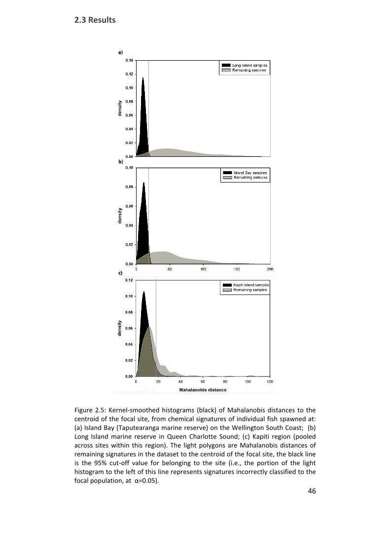
2.3 Results
46
Figure 2.5: Kernel-smoothed histograms (black) of Mahalanobis distances to the centroid of the focal site, from chemical signatures of individual fish spawned at: (a) Island Bay (Taputearanga marine reserve) on the Wellington South Coast; (b) Long Island marine reserve in Queen Charlotte Sound; (c) Kapiti region (pooled across sites within this region). The light polygons are Mahalanobis distances of remaining signatures in the dataset to the centroid of the focal site, the black line is the 95% cut-off value for belonging to the site (i.e., the portion of the light histogram to the left of this line represents signatures incorrectly classified to the focal population, at α=0.05).

Chapter 2. Scale-dependent variability in hatchling otolith chemistry
47
2.4 Discussion
2.4.1 Scaling of variability in hatchling otolith signatures
A complete description of connectivity in marine metapopulations
requires an understanding of all pair-wise larval exchanges between local
populations. Inferring such patterns from hatchling otolith microchemistry
depends upon unique trace element signatures across all sites within a
domain of interest (and across all sites in a natal atlas when recruits of
unknown origin are to be assigned to putative natal populations).
Despite the dissimilarity in geography, I observed scales of variability in
hatchling otolith signatures comparable to those found for the Galapagos
Islands and Hawaiian Islands (Ruttenberg & Warner 2006, Ruttenberg et al.
2008) as well as those found along the Oregon coast (Miller 2007a).
Though there were clear differences in trace element signatures of
hatchlings across small scales (e.g., between clutches within sites, and
between sites within regions) and large scales (e.g. between islands), I
failed to observe significant variability in signatures among regions within
islands. I used simulated annealing to redefine regions post hoc, and while
this improved the overall power of this approach (i.e., capturing additional
variability at regional scales), differences among regions within islands
were still not particularly strong. This suggests that, for this system, much
of the variability in trace element signatures recorded within the otoliths of
hatchlings is explained by processes occurring at large spatial scales (e.g.,
temperature/salinity gradients between north and south islands) and at
smaller spatial scales (e.g., variation in trace elements among sites and/or
females). When I restrict the focus to individual regions for instance, sites
are relatively distinct: within the Pelorus Sound embayment and for the
offshore island of Kapiti, sites can be discriminated amongst with some
confidence, despite some sites (e.g., Kapiti) being relatively close
geographically and not significantly different from each other.
2.4 Discussion
48
The a priori regional groupings reflected prior beliefs about processes
that may contribute to spatial variation in trace element signatures, such as
'polluted' and 'pristine' river inputs for Wellington Harbour and Pelorus
Sound respectively. However, my results suggest that this variation (and
presumably also the processes that shape this variation) act on scales that
differ from the a priori defined regions. The fact that the data do not allow
for accurate estimation of natal origins at the regional level of the natal
reference atlas may seem an important limitation of the hatchling otolith
approach for this system. I suggest that this limitation could be addressed
by adopting a Bayesian approach (Munch & Clarke 2008) that incorporates
prior knowledge of, e.g., local hydrodynamics, genetic information and
distributional maps of species. Explicitly and probabilistically integrating
such supplementary information could reduce uncertainty around natal
sources by adding confidence in assignments.
My analyses suggest that clutches collected from a common site vary
substantially in trace element signatures, and this is consistent with reports
from other systems (Warner et al. 2005, Ruttenberg & Warner 2006,
Ruttenberg et al. 2008). These differences possibly represent differential
maternal provisioning, and/or they may reflect fine scale variability in the
environment (Ruttenberg et al. 2005, Chittaro et al. 2006). Some trace
metals (e.g., Zn and Mn) act as cofactors in enzymatic reactions of
phytoplankton and may thus exhibit small scale variability with respect to
depth or sources of input and associated planktonic communities (Morel &
Price 2003).
A suite of elements was useful to discrimination at all scales. Since no
one element dominated the F statistics at any scale, or even over multiple
scales, my data suggest that multi-elemental signatures may enhance
discrimination. Variation in many of these elements may reflect differences
in water chemistry (e.g. Sr, Ba; (Elsdon & Gillanders 2005, Walther &

Chapter 2. Scale-dependent variability in hatchling otolith chemistry
49
Thorrold 2006) whereas variation in other elements may indicate
differences in physiology (perhaps mediated by spatial variation in water
temperature, genetic variation), or differential maternal investment; (e.g.
Chittaro et al. 2006, Thorrold et al. 2006). I note that a large part of the
variance in the dataset remains unexplained by the model. This may be due
to an inadequate model (e.g. the model structure does not reflect the
structure in the data), measurement noise, non-obvious contamination
and/or residual variation between hatchlings from a common clutch.
Additional research is needed to determine the underlying sources of
observed variability in trace element signatures across different spatial
scales (see also Elsdon et al. 2008).
Furthermore, my data do not allow me to examine temporal stability
in these signatures. Seasonal changes in environmental variables such as
temperature and freshwater runoff may alter site-specific patterns through
time, by influencing fish physiology (e.g. higher metabolic rates at higher
temperatures) and bioavailability of some elements (e.g. Elsdon &
Gillanders 2006). Although not a strict limitation to the use of core
signatures as markers of natal origin, temporal stability of some useful
elements would greatly facilitate the practical application of this approach.
Otherwise, atlases of natal signatures will have to be regenerated for each
subsequent recruitment event.
2.4.2 Optimal regional groupings by SA
Nearby sites in the atlas have considerably different signatures (as
evidenced from Fig. 4), and pooling these sites (without attention to this
underlying heterogeneity) would result in a group with large variance and
hence low overall classification success. In this case, the best groupings are
not obvious from a MDS plot of site centroids (Figure 2.4). I thus aimed to
optimize such clusters with respect to specific criteria, which can be
modified to suit a given ecological question at hand: one could, for

2.4 Discussion
50
example, leave out a location of interest, say a reserve or site of impact,
and then optimally group remaining sites to optimize resolution with
respect to desired predictive success.
While SA groupings did provide improvement for regional scale
allocation success and optimized signal to noise ratio (Figure 2.3), even
these optimal groupings did not achieve satisfactory allocation success at
this scale. Nevertheless, this approach allows exploring the limits of
resolution at a given scale and within a given dataset or for a given
ecological question. For the modified cost function, for instance, the
algorithm favoured small groups and thus a high resolution, which is
generally synonymous with a loss in predictive power in the LDA. Yet the
overall predictive success for the nine selected groupings was similar to
that of the six a priori defined regions. The groupings thus seem to be more
homogenous: no predictive power is lost by increasing the resolution with
respect to a priori defined regions.
2.4.3 Exclusion test
For some applications, such as dispersal from and/or to protected
populations whose viability might depend on external larval supply
(Stobutzki 2001, Halpern et al. 2006), it may be of interest to estimate
levels of self-recruitment versus external larval supply instead of explicitly
identifying precise source locations. This may be achieved by using an
exclusion test such as the one employed here. When considering a subset
of locations from the total dataset, exclusion of non-local signatures is
possible in certain settings where locations are sufficiently unique in their
signatures. For Long Island, Island Bay and Kapiti sites, three marine
reserves within the sampling domain, 95%, 85% and 76% of remaining
signatures can be excluded respectively, thus providing a way to estimate
larval supply to these marine reserves. If all other possible natal sites are
sampled within the range of dispersal of the species, one may by

Chapter 2. Scale-dependent variability in hatchling otolith chemistry
51
reciprocity also estimate larval supply from a marine reserve to
surrounding localities by applying this test.
In this case, when I employed such a test on a large scale, I quickly
became confronted with the problem of overlapping site distributions
between regions: the proportion of individuals correctly rejected becomes
very small as soon as I enlarge the focal area (location) to more than one
site (e.g. multiple sites within a region). In such circumstances the
application of an exclusion test would be misleading: failure to exclude a
large proportion of 'foreign' fish from a larger subset of focal sites would
result in an overestimate of self-recruitment. Standish et al. (2008) used a
similar approach to ours for excluding recruits from a set of three potential
source locations. However, no experimental tests were conducted on their
dataset and it is difficult to know how well their exclusion test performed.
The repeated tests with truncated datasets further revealed how
sampling effort is directly related to our ability to estimate the exclusion
potential of the test. In my case, I can drop two sites from my dataset
without dramatic changes in the percentage of correctly excluded
individuals. If I drop ten sites, however, these estimates diverge by as much
as 30%, depending on which sites remained in the sample. For cases in
which many sites with similar trace element signatures remained in the
sample, estimates of correctly excluded individuals were poor relative to
cases which included more heterogeneous sites. The likelihood of such
extreme samples therefore depends on the number of sites sampled, and
the extent of spatial covariance relative to the spacing of the sampled sites.
To make any claims about the ability of an exclusion procedure to correctly
exclude foreign signatures, the sample thus needs to encompass as much
of the variability in signatures found across the dispersal range of the focal
species as possible. Carefully considered sampling designs, e.g., informed
by preliminary pilot studies, can be extremely useful in this respect, and
2.4 Discussion
52
may lend increased confidence in the inferences derived from studies using
otolith chemistry.
2.4.4 Conclusion
The aim with this chapter was to investigate spatial scales of variability
in hatchling otolith signatures for this system, in the light of ecological
questions involving larval dispersal. I demonstrated that site differences in
an atlas of hatchling otolith signatures are exploitable at certain scales, the
usefulness of which depends on the ecological question at hand. On some
scales (regional scales in my system) supplementary information may help
to improve the strength of inferences of dispersal pathways. The exclusion
test provides a useful tool to assess larval subsidies from specific locations
(e.g., marine reserves) on small scales. On a large scale, hatchling otolith
microchemistry may yield insights into the question of present day
dispersal between the main islands of New Zealand. In the light of such
potential applications, further research into determinants of variability in
hatchling otolith chemical signatures seems warranted, and could
ultimately facilitate valuable insights into dispersal patterns in reef fish
metapopulations.

53
Chapter 3:
3. Characterizing natal sources of fish using
flexible Bayesian mixture models for otolith
geochemistry
3.1 Introduction
Geochemical tracers are increasingly used to reconstruct migrations
and estimate demographic connectivity in both terrestrial and marine
systems (Hobson 1999, Thorrold et al. 2002, Rubenstein & Hobson 2004,
Elsdon et al. 2008). Trace element tags contained within inert structures,
such as fish otoliths, mollusc statoliths or bird feathers, have been used to
quantify connectivity on ecological timescales (Swearer et al. 1999, Szép et
al. 2003, Zacherl 2005), and stable isotopes have been employed to study
migratory pathways of fish (Thorrold et al. 2001, Barnett-Johnson et al.
2008), birds (Rubenstein et al. 2002) and mammals (Burton & Koch 1999).
Inferences from such geochemical tags generally involve initial
sampling of individuals from populations of interest to establish a
geographical baseline, or reference “atlas”. Individuals of unknown origin
are then assigned to one of the populations in this reference atlas based on
their geochemical signature. This approach can illuminate dispersal
patterns and the underlying mechanisms that govern dispersal for a species
of interest by relating connectivity to environmental features (Schick et al.
3.1 Introduction
54
2008, Shima & Swearer 2009a, Swearer & Shima 2010). Insight gained
using geochemical tracers can thereby provide valuable insight about the
interaction between dispersal and population level outcomes (Hamilton et
al. 2008, Shima & Swearer 2009a, 2010).
The identifiability of potential source sites or source populations is a
major determinant of the success of such studies (Rubenstein & Hobson
2004, Elsdon et al. 2008). In some coastal marine environments, the
underlying environmental gradients can be gradual and/or populations
may be poorly resolved by geochemical tags (Elsdon et al. 2008,
Ruttenberg et al. 2008). Furthermore, such approaches generally require-
or at least (implicitly) assume that all potential sources have been sampled
in order to determine natal origins of recruits. Because comprehensive
sampling is often not feasible, the utility of this approach may be limited in
many marine environments (Campana et al. 2000, Munch & Clarke 2008,
White et al. 2008). Omission of potential source sites can limit the
inferences one can make regarding dispersal in a given system. In
particular, assignment of recruits to particular source sites may be
erroneous if one does not have a complete atlas. This may be of lesser
concern if there is spatial co-variation in signatures such that
misassignments are made to spatially neighbouring sources (Pella &
Masuda 2006).
A solution to this problem has been proposed in genetics (Cornuet et
al. 1999) and has recently been applied to otolith studies (Standish et al.
2008, Neubauer et al. 2010). The idea is to specify a criterion and to
calculate the distribution (by simulation or analytically) of this criterion for
the reference population. Based on this distribution, a threshold for
belonging to this population can be established. If any fish of unknown
origin falls outside of the, say, 95% confidence region of this distribution,
the individual remains unassigned. One could thus potentially exclude
Chapter 3. Bayesian mixture models for otolith geochemistry
55
individuals from populations that are not contained within the reference
atlas. An empirical evaluation of this approach however showed that this
method is only applicable on small scales in systems with a poorly resolved
reference atlas and may be of limited use for large scale connectivity
studies (Neubauer et al. 2010).
A different approach uses clustering methods to identify potential
groups within a sample of recruits, which in turn may be related to likely
geographical origins (White et al. 2008, Fontes et al. 2009, Shima &
Swearer 2009a). This alternative approach uses clustering of signatures
followed by a form of model selection to estimate the most likely number
of sources. If possible, the estimated clusters are then assigned to a given
source or a collection of sources. However, such post‐hoc interpretation of
clustering patterns can be difficult, especially for clustering approaches
which are not based on specific underlying models: it may not be clear
what the observed clusters represent, i.e. to what spatial scale the cluster
differences should be attributed, or whether clusters contain information
other than spatial patterns (i.e. physiological/maternal effects on otolith
chemistry). Most importantly, however, clustering methods do not use a
baseline to separate groups, but rather just find the most homogenous
groups within the individuals unknown origin. They are thus best suited for
problems in which a baseline is completely absent. This is showcased by
the classification results of the Bayesian clustering method presented in
White et al. (2008): the clustering method with post-hoc assignment to
sources often performs worse than linear discriminant analysis for
simulated datasets.
Bayesian tools have gained considerable ground in the analysis of
samples of mixed origin (i.e. stock mixtures in fisheries or recruits of
unknown origin in connectivity studies), mostly due to the possibility to
define realistic and probabilistically sound models which can incorporate
3.1 Introduction
56
uncertainty at various levels of an analysis (Pella & Masuda 2001, Manel et
al. 2005, Pella & Masuda 2006, Bolker et al. 2007, Munch & Clarke 2008,
White et al. 2008, Smith & Campana 2010). As others have pointed out (i.e.
Koljonen et al. 2005), most of these (as well as non-Bayesian methods) can
be classified as either conditional or unconditional models. In conditional
models, the baseline distributions (usually their mean and variance in
geochemical studies), once estimated, are considered fixed and estimation
of classification probabilities and mixing proportions are conditional on this
estimate. In unconditional models, the baseline and mixture parameters
are shared between the baseline and the mixed sample and are jointly
estimated from both datasets. Koljonen et al. (2005) found that such
methods usually perform better at mixed stock estimation tasks, due to the
fact that the information about the baseline inherent in the mixed sample
is used to better define their distributions. The models in this category can
be further divided into many-to-one and many-to-many analyses (Bolker et
al. 2007), depending on whether different mixed samples are considered
independently or jointly across different locations of collection,
respectively. This separation is meaningless in conditional models since the
mixed stocks do not influence the source distributions.
Bayesian methods have been proposed to provide an answer to the
problem of an unknown number of sources in a mixture. Pella & Masuda
(2001) proposed posterior predictive checks for an unconditional Bayesian
mixture model from genetic characteristics to identify potential
mismatches between the baseline and the mixed source sample. Smith &
Campana (2010) used these same checks for a joint model of otolith and
genetic data. Such a mismatch could indicate the presence of un-sampled
sources in the mixed sample. It does not, however, provide a way to
estimate the nature and number of such extra-baseline populations.
Chapter 3. Bayesian mixture models for otolith geochemistry
57
A Bayesian method to directly identify the contribution of extra-
baseline sources to a mixture is provided by Pella & Masuda (2006). Their
use of a prior which has support over a theoretically infinite number of
possible sources elegantly sidesteps the problem of model selection and
provides a marginal distribution over the number of sources in the mixed
sample. My focus in this chapter is to develop analogous models for
geochemical data that follow the distribution assumptions commonly
employed for this kind of data. I start by outlining Bayesian methods that
extend parametric cluster analysis (White et al. 2008) by employing non‐
parametric Bayesian priors, and specifically Dirichlet Process priors (DP)
(Escobar & West 1995). Loosely speaking, non‐parametric Bayes provides a
flexible framework by formulating priors over model space, such as over
models with different numbers of source populations. In this context, the
DP model can be used to directly infer the number of possible natal
sources in a mixture model if no baseline is available. I obtain marginal
posterior distributions of the number of sources and marginal
representations of relatedness of individuals in terms of their geochemical
signatures. This framework is then extended to include baseline samples in
an unconditional analysis which classifies fish with either the baseline
samples or out-of-sample classes. In an extension of the method proposed
by Pella & Masuda (2006), I describe different ways in which a mixed
sample can be clustered with such a baseline. Lastly, I propose a new
method for hierarchical unconditional classification, which can be used
with an incomplete reference atlas. This model employs a classification
procedure at large scales and an embedded non‐parametric clustering at
smaller scales. These models are tested on the well-known weakfish data
set (Thorrold et al. 2001), which has been previously evaluated by other
authors to illustrate Bayesian methods for otolith data (Munch & Clarke
2008, White et al. 2008).
3.2 Statistical models
58
3.2 Statistical models
3.2.1 A Dirichlet process mixture (DPM) model for clustering
In this section I introduce the DPM, an extension of the finite mixture
model commonly employed in mixed sample analyses. The goal of this
model is similar to that of White et al. (2008) and the model has many of
the same limitations, but an analytical integration step makes it possible to
circumvent the problem of model selection in mixture models and to infer
the number of potential sources directly.
I assume that the p-dimensional vector of geochemistry data for
individuals i = (1:::N )i = (1:::N ) , denoted yi = (yi;1; : : : ; yi;p)yi = (yi;1; : : : ; yi;p) , comes from an
unknown underlying multivariate normal distribution N (µi)N (µi), where the set
µi = f¹i;§2igµi = f¹i;§2ig includes the mean vector and covariance matrix for the
distribution of yiyi. Furthermore, the µiµi are drawn from a mixing distribution
GG, itself drawn from a Dirichlet Process, a distribution over individual
source distributions in the mixed sample. The hierarchical version of this
model can be written as (Neal 2000):
yijµi » N(µi)
µijG » G
G » DP (°; G0)
yijµi » N(µi)
µijG » G
G » DP (°; G0) (3.1)
The Dirichlet Process is parameterized by G0G0 and °°. G0G0 is called the
base measure for the source specific multivariate normal distributions: it is
the prior expectation of GG such that E[G(µ)] = G0(µ)E[G(µ)] = G0(µ). The °° parameter
measures how centred source distribution parameters are around the base
distribution G0G0, as demonstrated below, and determines the number of
sources in the model. A small °° is synonymous with few sources and vice‐
versa. The DPM can be derived in a number of ways, leading to equivalent
distributions over partitions of the data. The most appropriate in the
context of the mixed sample problem in fisheries and ecology is a

Chapter 3. Bayesian mixture models for otolith geochemistry
59
derivation of the DPM as the infinite limit of the finite mixture model (Neal
1992, Neal 2000). In this view we have a theoretically infinite number of
sources that could contribute to a sample. In practice only a limited
number of sources will contribute to the mixed sample, as detailed below.
The most important feature of this model is the discreteness of the
draws from a DPDP : values drawn from the DPDP will have positive probability
to coincide. In other words, some individuals will share a common
parameter vector µµ, indicating that they originate from the same source.
This is the basis for clustering in the model. To see this, consider the prior
for µµ that arises if GG is integrated out of the model. This can be shown to
be a series of draws from the conditional distribution of µiµi given all other
µ¡iµ¡i (Ferguson 1973):
µijµ¡i; ° »
1
N ¡ 1 + °
NX
j 6=i
±(µj) +°
N ¡ 1 + °G0µijµ
¡i; ° »1
N ¡ 1 + °
NX
j 6=i
±(µj) +°
N ¡ 1 + °G0 (3.2)
where ±(µj)±(µj) is a point mass at µjµj. This is a mixture formulation: with
probability proportional to °° a new instance of µµ will be drawn from G0G0,
else µiµi will coincide with one of the jj previous instances of µµ. From this
formulation it is clear that the number of sources drawn in this model will
be finite in practice.
This conditional formulation of the DPDP prior is very useful in
another way: it makes drawing samples form the posterior distribution of
the DPM model given the data YY rather straightforward. Note that (3.2) is
only the conditional prior distribution of µiµi and that Bayes theorem will
combine it with the likelihood P (yijµi)P (yijµi) to give the posterior distribution of
the source parameters µiµi. The source parameters µiµi do not need to be
sampled explicitly; it is often easier to obtain samples from source
assignments cici to source kk (though they are readily obtainable from the
conjugate construction employed below if needed). This is so because the

3.2 Statistical models
60
µiµi which coincide define a source membership, and the actual source
parameters can be integrated out of the model, as in Munch & Clark
(2008). This integration makes Gibbs sampling more effective as it limits
the number of states of the sampler. The conditional prior given above can
then be written in terms of individual source assignments:
p(ci = kjc¡i; °) =
(n¡i
k
n¡1+°; k · K+
°
n¡1+°; k > K+
p(ci = kjc¡i; °) =
(n¡i
k
n¡1+°; k · K+
°
n¡1+°; k > K+
where K+K+ is the number of sources currently associated with an
observation and n¡ikn¡ik is the number of individuals associated with source kk
except individual ii. The prior is similar in interpretation to the classical
mixture proportion in finite mixture models: the larger the proportion n=Nn=N
of individuals assigned to a given source, the larger the prior probability
that the next individual considered will come from this source as well. To
sample from the full posterior distribution one can alternate Gibbs
sampling of source assignments and sampling of °° , which is directly
analogous to sampling in finite mixtures (see for instance the Gibbs
sampler in Munch & Clarke 2008). To sample source identities, the prior for
the i‐th observation is combined with its likelihood and the following
probabilities can be used to draw samples of assignments c= c1:::ci:::cnc= c1:::ci:::cn,
(Neal 2000):
p(ci = kjc¡i; °; Y ) = ®
(n¡i
k
n¡1+°
RN(yijµk)dH¡i(µk); k · K+
°
n¡1+°
RN(yijµk)dG0(µk); k > K+
p(ci = kjc¡i; °; Y ) = ®
(n¡i
k
n¡1+°
RN(yijµk)dH¡i(µk); k · K+
°
n¡1+°
RN(yijµk)dG0(µk); k > K+
(3.3)
where H¡i(µk)H¡i(µk) is the posterior distribution of µkµk given data yc¡ik
yc¡ik
, is the data
of all fish associated with source kk except the data of fish ii. ®® is a constant
assuring that this probability integrates to 1. I use a vague multivariate-
Normal-inverse-Wishart conjugate prior for G0G0, which makes it possible to
solve the integration over µµ analytically. This prior has four parameters, the
prior mean ¹0¹0 and scale matrix ¢0¢0 as well as the prior degrees of freedom
Chapter 3. Bayesian mixture models for otolith geochemistry
61
for the scale matrix (º0º0) and a prior parameter ·0·0 which relates the variance
of ¹k¹k to §k§k . RF(yijµk)dH¡i(µk)
RF(yijµk)dH¡i(µk) is then a multivariate student‐t density for
source assignments with parameters updated according to the observed
data (Gelman et al. 2003):
yijyc¡ik; G0 » tºn¡D+1(¹n;¢n(·n + 1)=·n(ºn +D + 1))
¹n =k0
k0 +N¹0 +
n¡ickk0 + n¡ick
yc¡ik
·n = ·0 + n¡ick
ºn = º0 + n¡ick
¢n = ¢0 + SSc¡ik
+·0n
¡ick
·0 + n¡ick(yc¡i
k¡ ¹0)(yc¡i
k¡ ¹0)
T
yijyc¡ik; G0 » tºn¡D+1(¹n;¢n(·n + 1)=·n(ºn +D + 1))
¹n =k0
k0 +N¹0 +
n¡ickk0 + n¡ick
yc¡ik
·n = ·0 + n¡ick
ºn = º0 + n¡ick
¢n = ¢0 + SSc¡ik
+·0n
¡ick
·0 + n¡ick(yc¡i
k¡ ¹0)(yc¡i
k¡ ¹0)
T (3.4)
The subscript 00 denotes the prior value for the parameter, and SS is
the sum of squares within the considered source. The second case in
(3.3) defines a new source, the µkµk is therefore defined by the observation
yiyi alone, and K+K+ is augmented by 1 if this case is drawn. Integrating with
respect to the prior G0G0 gives the same predictive likelihood as before with
yiyi as the sole observation of the new class, and the prior parameters
determine the predictive likelihood in (3.4). Finally, °° is estimated from
data using Gibbs sampling procedures described in Escobar & West (1995),
using a vague Gamma(1,1) distribution as prior. The conditional posterior is
then a mixture of Gamma distributions:
°j»; k » ¼»G(1 + k; 1¡ log(»)) + (1¡ ¼»)G(1 + k ¡ 1; 1¡ log(»))°j»; k » ¼»G(1 + k; 1¡ log(»)) + (1¡ ¼»)G(1 + k ¡ 1; 1¡ log(»))
where »» follows a beta distribution such that »j°; k » B(° + 1; N)»j°; k » B(° + 1; N) and
¼» =(K+¡K+log(»))=(K+¡K+log(»)+N)¼» =(K+¡K+log(»))=(K+¡K+log(»)+N)
Posterior estimation can be difficult in the DPM when the posterior
is multimodal, which is the case with any mixture model estimated with
latent (unknown) classes. Since the labels of assignments cc are irrelevant
to the actual estimation, the model is said to be invariant with respect to

3.2 Statistical models
62
the class labels. One would thus obtain the same partition into clusters
with every combination of class labels, such that for KK sources there
would be K!K! different posterior modes. The Gibbs sampler has a tendency
to remain in one of these modes and often does not explore the posterior
distribution properly. This occurs because the steps necessary to switch
between class labels have very low probability of occurring. Only using the
Gibbs sampling described above may therefore not guarantee adequate
sampling from that the posterior distribution (Jain & Neal 2004). To ensure
adequate mixing of the sampler I coupled the Gibbs sampler over only C
and °° with a split‐merge sampling step (Jain & Neal 2004). A split merge
step helps the sampler pass regions of low posterior probability in
parameter space, thereby improving sampling from the full posterior. This
is achieved by splitting or merging clusters formed by Gibbs sampling,
where splits or merges are accepted with a Metropolis‐Hastings
acceptance probability to ensure convergence to the stationary
distribution (Jain & Neal 2004). Specifically, I used the improved split‐
merge procedure with sequential allocation (Dahl 2003) to achieve optimal
performance of the sampling scheme. For a detailed discussion of this
sampler in the context of mixed stocks from a genetic perspective, see
Pella & Masuda (2006). Changing the likelihood to that corresponding to
(4) gives a direct correspondence of their sampling scheme with the one
used for this study. All inferences presented in this paper are based on
10000 samples from the posterior distribution of the model after a burn-in
of 1000 samples was discarded. Convergence of the Markov chains was
checked visually and confirmed from multiple starts with random initial
conditions.
3.2.2 Using the DPM with a baseline
The above stated DPM model can be applied as such, without a
baseline. It is however straightforward to appreciate why this is difficult
and of limited use with otolith chemistry: the number of sources selected
Chapter 3. Bayesian mixture models for otolith geochemistry
63
by the model will depend on the prior for the covariance matrix. If the prior
is vague, the covariance matrix needs to be estimated from data, which
may be difficult when the data are not clearly separated. As a result it will
be difficult to know to which spatial scale the estimated number of sources
pertains. To extend the use of the DPM, I propose two separate ways to
use this model with a baseline: 1) in a clustering and 2) in a classification
(or discrimination) context. The latter has been discussed by Pella and
Masuda (2006) with genetic data. It consists of applying the DPM to the
mixed sample with a certain number of fixed populations. Sampled
individuals are assigned to either an existing source or an extra-baseline
source in the Gibbs sampler. The probability that this individual comes
from one of the proposed sources or from an un-sampled baseline source
can then be estimated. Incorporation of the baseline into the sampling
scheme described above is straightforward and the necessary additions are
detailed by Pella and Masuda (2006).
In some applications however, we may know (e.g. from cross-
validation studies) that assignment success to one of the baseline
populations will be rather low. This is often due to limited resolution in the
dataset, but as illustrated elsewhere (Smouse et al. 1982, Neubauer et al.
2010), a large number of baseline sources can make assignment difficult
even with good local resolution – all else being equal, assignment success
will generally decrease with an increasing number of sources considered.
Furthermore, using otolith chemistry to define a source population may
lead to multimodal distributions if variation occurs on scales smaller than
the one on which a source is defined (see discussion). In some instances we
may thus have little confidence in the actual assignments to the baseline
sources if these are highly resolved (i.e. individual embayments or islands)
(Warner et al. 2005, Ruttenberg & Warner 2006, Ruttenberg et al. 2008,
Neubauer et al. 2010). I propose that in such instances a DPM clustering of
the mixed sample (or recruits) of unknown origin with the baseline as a
3.2 Statistical models
64
joint dataset may provide more insight. For some regions in parameter
space some individual sources may be rather well defined and some
clusters will therefore consist of individuals from a single source, adjacent
sources, or perhaps a regional source pool (see, for instance, White et al.
2008). Mixed samples which are clustered within such pure clusters can
therefore be regarded as more certain classifications, samples within mixed
clusters will represent uncertain classifications. This feature is illustrated
below on the weakfish dataset.
3.2.3 Extension to hierarchical classification with an incomplete
atlas
The DPM essentially performs a model-based clustering where the
number of clusters is a marginal quantity of the posterior distribution of
the model. Basing the clustering on such a model can provide distinct
advantages, the most relevant of which is that the number of sources does
not need to be specified, nor do we need to define a criterion to find the
most likely number of such sources. Here, I take this approach a step
further and embed the DPM clustering model detailed above in a
classification model. I propose to perform classification on a continuous
map, for instance at the scale of regions within the total sampled area,
where each region is modelled by a Dirichlet Process mixture of its
individually sampled sources (Figure 3.1a). In other words, I replace the
commonly used normal density in a (Bayesian) mixture or discriminant
analysis for otolith chemistry (or other continuous data) by a mixture
density.
Formally, classification within a discriminant analysis or mixture model
involves the use of Bayes theorem to calculate posterior assignment
probabilities
p(³i = qjyi) =f(yijµq)¼q
PQ
q0=1 f(yijµq0)¼q0p(³i = qjyi) =
f(yijµq)¼qPQ
q0=1 f(yijµq0)¼q0

Chapter 3. Bayesian mixture models for otolith geochemistry
65
where ³i³i assigns a source qq to fish ii, based on the likelihood f (yijµq)f (yijµq) of fish
ii given the source specific parameters µqµq and a specified prior ¼q¼q
(amounting to a discriminant analysis) or estimated mixture proportion ¼q¼q
(the mixture model setup) for sources in the baseline. The normal density
is often used to define the likelihood for such a classification with
continuous data, with µqµq estimated from baseline data (Munch & Clarke
2008, White et al. 2008). The central limit theorem assures that the sum of
independently drawn random variables is normal and thus even if
differences exist on scales smaller than the one on which we define a
source, the data will be asymptotically normal if a large number of fish
from each source are sampled. Since this result holds only asymptotically
however, we may in practice see multimodal distributions at the randomly
defined scales at which regions or sources are delimited. For instance, a
source may be defined over a stretch of coast or a spawning site which
receives local freshwater input or experiences a localized upwelling. One
may then expect some elements (i.e. Barium) to be significantly different
between individuals that experienced such an anomaly within the source,
and the distribution would be bi-modal at the scale of the source. The
normal distribution may in that case be a poor approximation of the true
density of each source.
The main idea behind the classification model proposed here is to
subdivide the entire region of study (the region that may contribute to
local recruit pools) into contiguous but adjacent regions (see Figure 3.1 for
an illustration of this method), each of which is modelled by a DPM. This
could be especially useful for hierarchically structured datasets (i.e.
Ruttenberg & Warner 2006, Miller 2007b, Ruttenberg et al. 2008,
Neubauer et al. 2010). If each region has been sampled representatively, it
may then be possible to estimate contributions from these QQ regions to a
recruit pool. This reasoning applies to any classification procedure. Indeed,
even a single sampling site is an arbitrarily scaled region, and problems
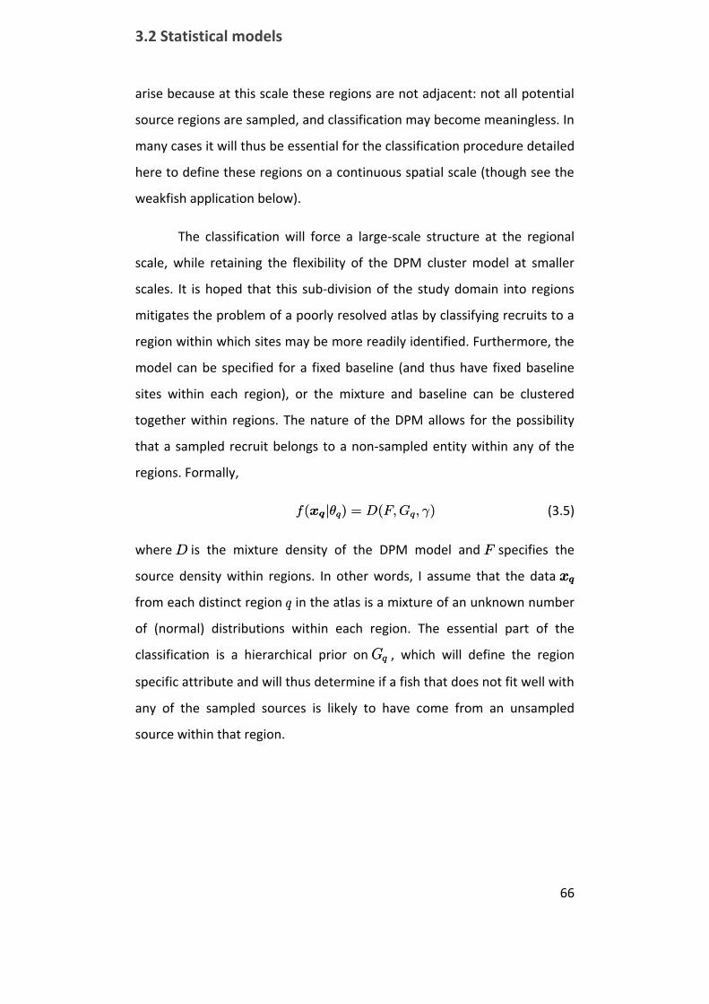
3.2 Statistical models
66
arise because at this scale these regions are not adjacent: not all potential
source regions are sampled, and classification may become meaningless. In
many cases it will thus be essential for the classification procedure detailed
here to define these regions on a continuous spatial scale (though see the
weakfish application below).
The classification will force a large-scale structure at the regional
scale, while retaining the flexibility of the DPM cluster model at smaller
scales. It is hoped that this sub‐division of the study domain into regions
mitigates the problem of a poorly resolved atlas by classifying recruits to a
region within which sites may be more readily identified. Furthermore, the
model can be specified for a fixed baseline (and thus have fixed baseline
sites within each region), or the mixture and baseline can be clustered
together within regions. The nature of the DPM allows for the possibility
that a sampled recruit belongs to a non-sampled entity within any of the
regions. Formally,
f(x jµq) = D(F;Gq; °)f(x jµq) = D(F;Gq; °) (3.5)
where DD is the mixture density of the DPM model and FF specifies the
source density within regions. In other words, I assume that the data xx
from each distinct region qq in the atlas is a mixture of an unknown number
of (normal) distributions within each region. The essential part of the
classification is a hierarchical prior on GqGq , which will define the region
specific attribute and will thus determine if a fish that does not fit well with
any of the sampled sources is likely to have come from an unsampled
source within that region.
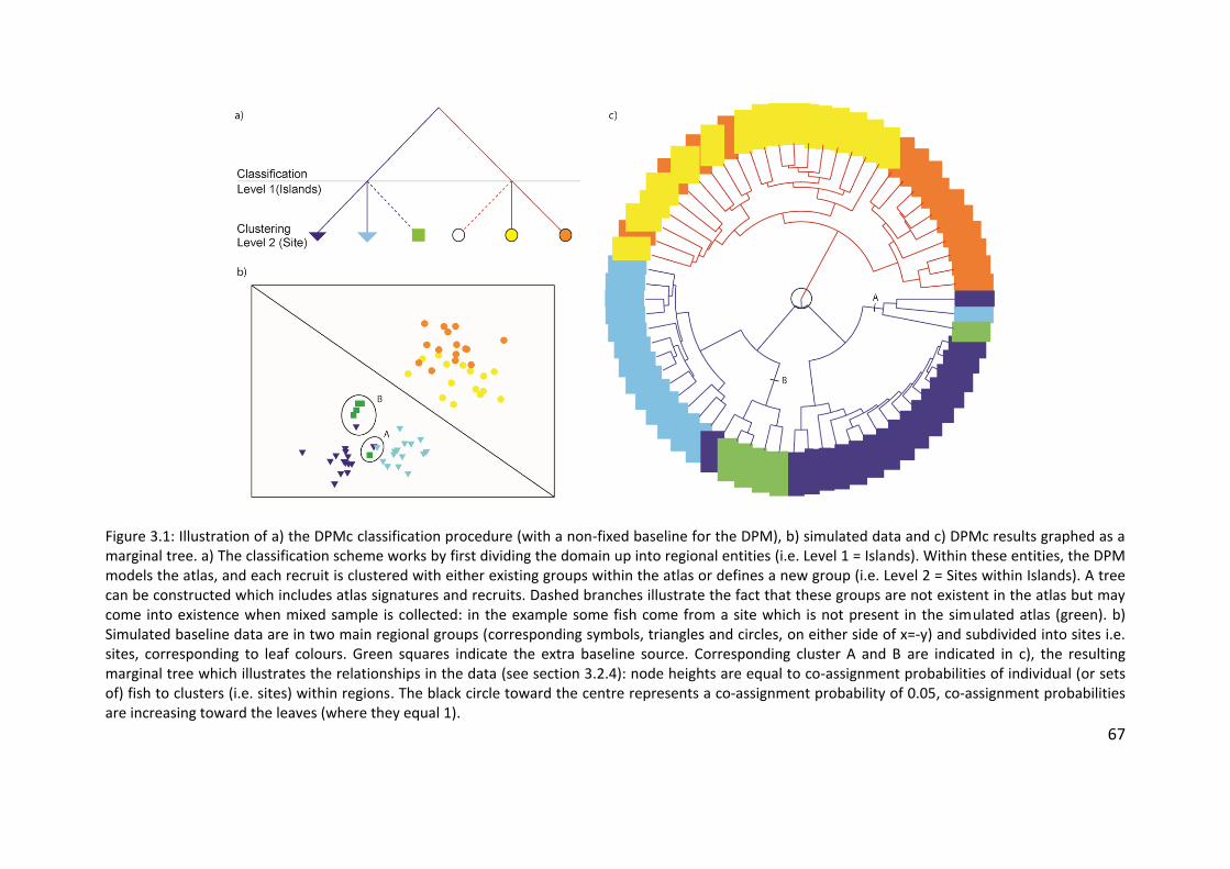
67
Figure 3.1: Illustration of a) the DPMc classification procedure (with a non-fixed baseline for the DPM), b) simulated data and c) DPMc results graphed as a marginal tree. a) The classification scheme works by first dividing the domain up into regional entities (i.e. Level 1 = Islands). Within these entities, the DPM models the atlas, and each recruit is clustered with either existing groups within the atlas or defines a new group (i.e. Level 2 = Sites within Islands). A tree can be constructed which includes atlas signatures and recruits. Dashed branches illustrate the fact that these groups are not existent in the atlas but may come into existence when mixed sample is collected: in the example some fish come from a site which is not present in the simulated atlas (green). b) Simulated baseline data are in two main regional groups (corresponding symbols, triangles and circles, on either side of x=‐y) and subdivided into sites i.e. sites, corresponding to leaf colours. Green squares indicate the extra baseline source. Corresponding cluster A and B are indicated in c), the resulting marginal tree which illustrates the relationships in the data (see section 3.2.4): node heights are equal to co-assignment probabilities of individual (or sets of) fish to clusters (i.e. sites) within regions. The black circle toward the centre represents a co‐assignment probability of 0.05, co-assignment probabilities are increasing toward the leaves (where they equal 1).
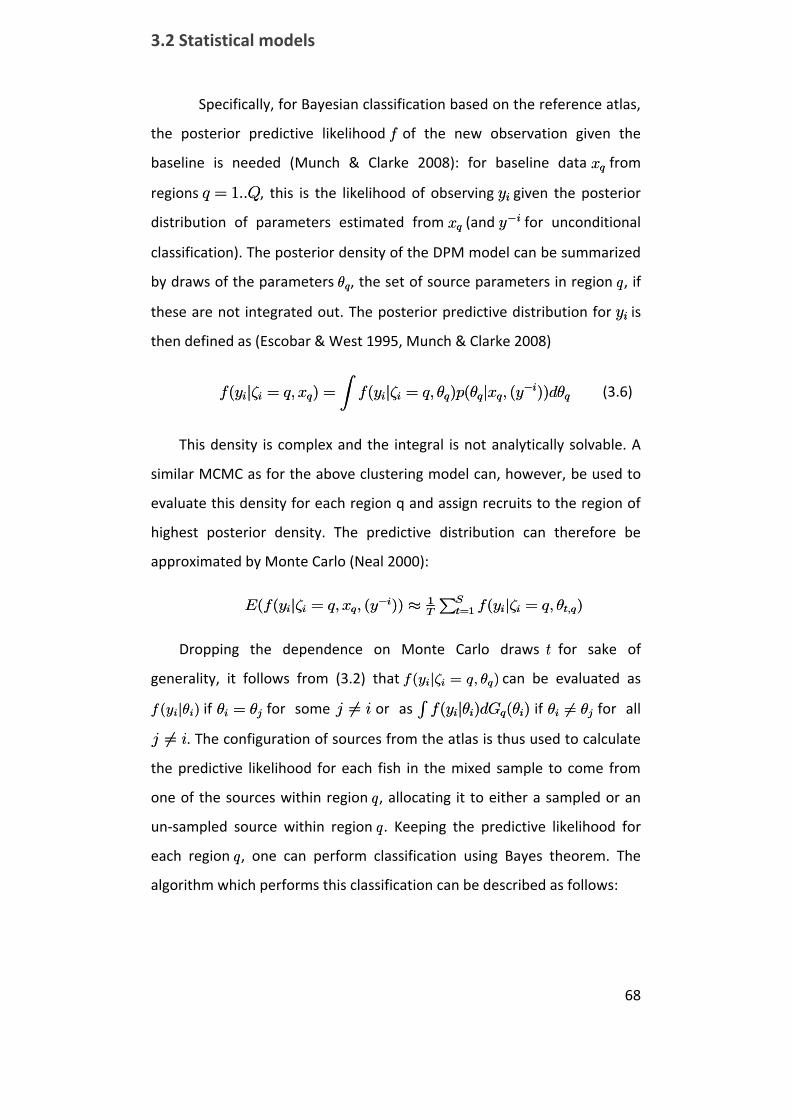
3.2 Statistical models
68
Specifically, for Bayesian classification based on the reference atlas,
the posterior predictive likelihood ff of the new observation given the
baseline is needed (Munch & Clarke 2008): for baseline data xqxq from
regions q = 1::Qq = 1::Q, this is the likelihood of observing yiyi given the posterior
distribution of parameters estimated from xqxq (and y¡iy¡i for unconditional
classification). The posterior density of the DPM model can be summarized
by draws of the parameters µqµq, the set of source parameters in region qq, if
these are not integrated out. The posterior predictive distribution for yiyi is
then defined as (Escobar & West 1995, Munch & Clarke 2008)
f(yij³i = q; xq) =
Z
f(yij³i = q; µq)p(µqjxq; (y¡i))dµqf(yij³i = q; xq) =
Z
f(yij³i = q; µq)p(µqjxq; (y¡i))dµq (3.6)
This density is complex and the integral is not analytically solvable. A
similar MCMC as for the above clustering model can, however, be used to
evaluate this density for each region q and assign recruits to the region of
highest posterior density. The predictive distribution can therefore be
approximated by Monte Carlo (Neal 2000):
E(f(yij³i = q; xq; (y¡i)) ¼ 1
T
PS
t=1 f(yij³i = q; µt;q)E(f(yij³i = q; xq; (y¡i)) ¼ 1
T
PS
t=1 f(yij³i = q; µt;q)
Dropping the dependence on Monte Carlo draws tt for sake of
generality, it follows from (3.2) that f(yij³i = q; µq)f(yij³i = q; µq) can be evaluated as
f (yijµi)f (yijµi) if µi = µjµi = µj for some j 6= ij 6= i or as Rf(yijµi)dGq(µi)
Rf(yijµi)dGq(µi) if µi 6= µjµi 6= µj for all
j 6= ij 6= i. The configuration of sources from the atlas is thus used to calculate
the predictive likelihood for each fish in the mixed sample to come from
one of the sources within region qq, allocating it to either a sampled or an
un-sampled source within region qq. Keeping the predictive likelihood for
each region qq, one can perform classification using Bayes theorem. The
algorithm which performs this classification can be described as follows:
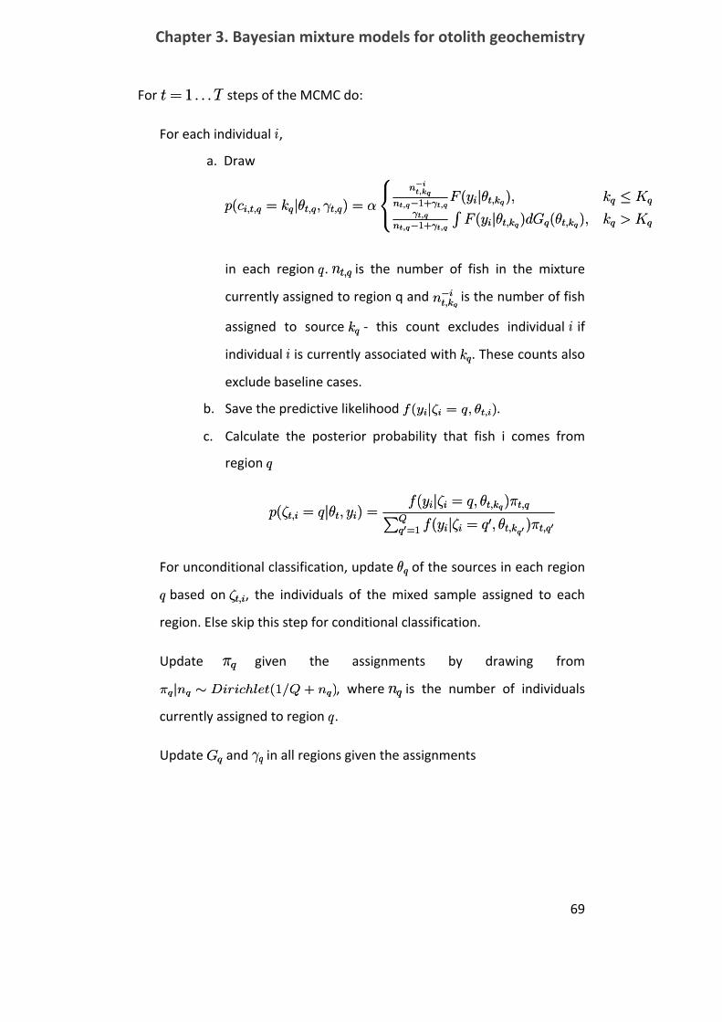
Chapter 3. Bayesian mixture models for otolith geochemistry
69
For t=1 : : :Tt=1 : : :T steps of the MCMC do:
1. For each individual ii,
a. Draw
p(ci;t;q = kqjµt;q; °t;q) = ®
8<
:
n¡it;kq
nt;q¡1+°t;qF (yijµt;kq
); kq · Kq
°t;q
nt;q¡1+°t;q
RF (yijµt;kq
)dGq(µt;kq); kq > Kq
p(ci;t;q = kqjµt;q; °t;q) = ®
8<
:
n¡it;kq
nt;q¡1+°t;qF (yijµt;kq
); kq · Kq
°t;q
nt;q¡1+°t;q
RF (yijµt;kq
)dGq(µt;kq); kq > Kq
in each region qq. nt;qnt;q is the number of fish in the mixture
currently assigned to region q and n¡it;kqn¡it;kq
is the number of fish
assigned to source kqkq - this count excludes individual ii if
individual ii is currently associated with kqkq. These counts also
exclude baseline cases.
b. Save the predictive likelihood f(yij³i = q; µt;i)f(yij³i = q; µt;i).
c. Calculate the posterior probability that fish i comes from
region qq
p(³t;i = qjµt; yi) =f(yij³i = q; µt;kq
)¼t;qPQ
q0=1 f(yij³i = q0; µt;kq0 )¼t;q0
p(³t;i = qjµt; yi) =f(yij³i = q; µt;kq
)¼t;qPQ
q0=1 f(yij³i = q0; µt;kq0 )¼t;q0
2. For unconditional classification, update µqµq of the sources in each region
qq based on ³t;i³t;i, the individuals of the mixed sample assigned to each
region. Else skip this step for conditional classification.
3. Update ¼q¼q given the assignments by drawing from
¼qjnq » Dirichlet(1=Q + nq)¼qjnq » Dirichlet(1=Q + nq), where nqnq is the number of individuals
currently assigned to region qq.
4. Update GqGq and °q°q in all regions given the assignments
3.2 Statistical models
70
3.2.4 Marginal descriptions of source assignments
Mixture models are prone to label switching, a phenomenon which
occurs during iterative estimation routines of latent (unobserved) class
models. The actual labels of these classes are arbitrary and switch
throughout the estimation routine. Unless one adopts a restrictive
formulation, DPMs also exhibit this property. To deal with this problem, a
re‐labelling algorithm to recover the most probable labels can be used (e.g.
White et al. 2008). Such procedures are not without pitfalls (see for
instance Dawson & Belkhir 2009 for available approaches for dealing with
the label switching issue and a discussion of these).
I follow Dawson & Belkhir (2009) and circumvent this problem by
noting that the sources are only defined by the observations (or
specifically, individual fish) that constitute them. Marginal posterior co‐
assignment probabilities of individuals that are invariant to label switching
can be obtained to express the degree of their similarity (Huelsenbeck &
Andolfatto 2007, Dawson & Belkhir 2009). This quantity expresses the
probability that two individuals (or a set thereof) are assigned to the same
cluster (or source in this case), given the uncertainty about the number and
nature of these clusters. It is therefore a marginal probability: it integrates
over the posterior distribution of model parameters, and thereby takes
into account the uncertainty inherent in this distribution.
To visualize patterns in the collected recruits from each site, I applied
the exact linkage algorithm of Dawson & Belkir (2009), which constructs a
tree (akin to a hierarchical clustering tree) based on estimates of marginal
co‐assignment probabilities. These probabilities are the probability that
two fish or sets of fish come from the same source given all uncertainty
inherent in model parameters. The node height of any node in the
constructed tree is the estimated posterior co‐assignment probability of
the sets which are merged by that node. One can then look for marginally
Chapter 3. Bayesian mixture models for otolith geochemistry
71
significant groups: these are clusters in the tree which are co‐assigned with
probabilities smaller than some threshold, say pc = 0:05pc = 0:05 . Since co‐
assignment probabilities integrate over uncertainty in the model
parameters and number of sources, these marginal co-assignment
probabilities can be regarded as minimal co-assignment probabilities. We
can therefore expect only well resolved sources to be significantly different
at this level.
I use a similar logic in dealing with output from the classification
procedure. Here, I aim to construct a tree that gives co‐assignment
probabilities given not only the uncertainty about sources within each
region, but which further marginalizes over classification probabilities to
these regions. For this, I cluster the mixed sample with atlas signatures of
the region which recruits were assigned to at each iteration of the MCMC
algorithm. This procedure marginalizes over classification assignment
probabilities and the exact linkage algorithm can be applied to construct a
tree. This can provide substantial information in the case of an incomplete
atlas. An illustration of this is given in the simulated classification example
(Figure 3.1c). Tree plotting and annotation was performed using TreeDyn
(Chevenet et al. 2006).
3.3 Application
3.3.1 DPM clustering models
To illustrate the DPM clustering method, I tested models with and
without baseline on the weakfish dataset of Thorrold et al. (2001). The
premise of the original study was to investigate philopatry in weakfish
using otolith core signatures of adult weakfish which were compared to a
baseline of otolith chemistries collected from juvenile weakfish two years
earlier. The authors use a discriminant analysis to assign adults to natal
estuaries, thus assuming that i) adult fish were spawned in one of five

3.3 Application
72
baseline estuaries and ii) that these estuaries were sufficiently
characterized by the data collected from juvenile fish to allow for such a
classification.
There are a number of motivations for using DPM models for a re-
analysis of this dataset. i) Recent models developed for assigning natal
origins (or estimating source proportions) based on otolith chemistry, have
used this dataset for illustrative purposes (Munch & Clarke 2008, White et
al. 2008). ii) While the original study notes that the five estuaries under
investigation account for 90% of commercial weakfish catch, other
estuaries along the east coast could have potentially accounted for some of
the adult fish in this study. iii) Some of these estuaries are relatively large
(i.e. Chesapeake Bay is the largest estuary in the USA), and large variation
in otolith chemistry can often be found even on small scales within
estuaries (Miller 2007a). This could lead to multi-modal distributions within
estuaries and the normal distributions used in previously applied models
may be a poor fit.
Thorrold et al. (2001) use chemistry measured from whole otoliths for
the juvenile baseline, whereas chemical measures on adult fish otoliths
were from the core only. I found that values for Magnesium were higher
within cores of adult otoliths than in whole juvenile otoliths. Recent studies
suggest that many elements are elevated in the otolith core of many
species (i.e. Mg, Mn, Ba (Brophy et al. 2004, Ruttenberg et al. 2005)). An
ontogenetic signal and/or a difference in sampling methods for juvenile
fish may therefore have led to lower Mg values in the reference atlas. Mg
was hence excluded from the analysis (to little overall effect).
3.3.2 Clustering fish without a baseline
I started by investigating whether the DPM model without a baseline
would successfully separate the baseline (juvenile fish from known
locations) into the five estuaries that were sampled. For this I used a vague
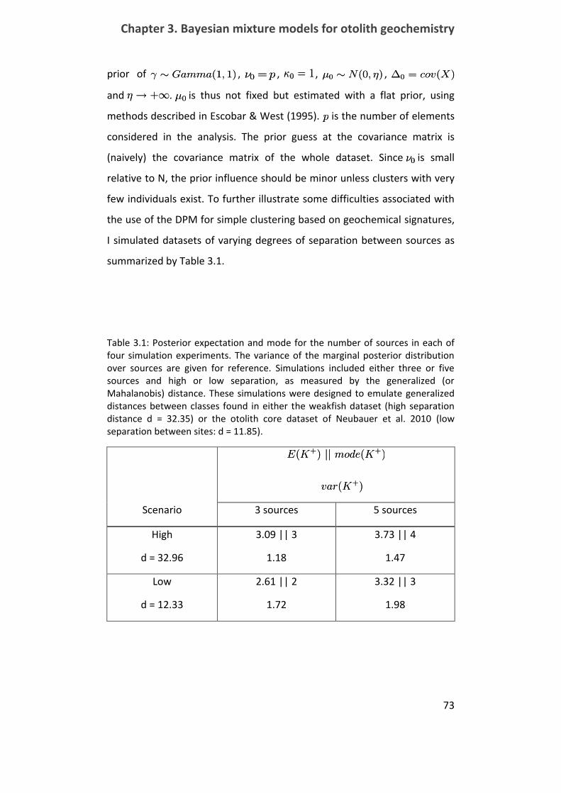
Chapter 3. Bayesian mixture models for otolith geochemistry
73
prior of ° » Gamma(1; 1)° » Gamma(1; 1) , º0 = pº0 = p , ·0 = 1·0 = 1 , ¹0 » N(0; ´)¹0 » N(0; ´) , ¢0 = cov(X)¢0 = cov(X)
and ´ ! +1´ ! +1. ¹0¹0 is thus not fixed but estimated with a flat prior, using
methods described in Escobar & West (1995). pp is the number of elements
considered in the analysis. The prior guess at the covariance matrix is
(naively) the covariance matrix of the whole dataset. Since º0º0 is small
relative to N, the prior influence should be minor unless clusters with very
few individuals exist. To further illustrate some difficulties associated with
the use of the DPM for simple clustering based on geochemical signatures,
I simulated datasets of varying degrees of separation between sources as
summarized by Table 3.1.
Table 3.1: Posterior expectation and mode for the number of sources in each of four simulation experiments. The variance of the marginal posterior distribution over sources are given for reference. Simulations included either three or five sources and high or low separation, as measured by the generalized (or Mahalanobis) distance. These simulations were designed to emulate generalized distances between classes found in either the weakfish dataset (high separation distance d = 32.35) or the otolith core dataset of Neubauer et al. 2010 (low separation between sites: d = 11.85).
E(K+) jj mode(K+)
var(K+)
E(K+) jj mode(K+)
var(K+)
Scenario 3 sources 5 sources
High
d = 32.96
3.09 || 3
1.18
3.73 || 4
1.47
Low
d = 12.33
2.61 || 2
1.72
3.32 || 3
1.98

3.3 Application
74
Analysis of simulated data showed that even with high overall separation in
the dataset the model does not necessarily recover the correct number of
sources (as indicated by the posterior mode) (Table 3.1), though the
correct number is generally within the 95% credible interval. The
performance naturally deteriorates when separation between sources is
lower. In fact, the distribution over sources depends solely on the
configuration of sources in multivariate space. If only two sources are very
similar, the correct number of sources will likely not be recovered.
Individual pairwise generalized distances in the simulation with high
separation ranged from 10.12 – 81.48, as compared to 6.06 – 83.21 in the
original weakfish dataset. Surprisingly, when applying the DPM to the
weakfish baseline, I find that the number of sources estimated from the
model are too high rather than too low (E(K+) = 7:63E(K+) = 7:63, Figure 3.2). Some
multi-modality is thus evident at the baseline level.
Figure 3.2: Histogram of the marginal posterior distribution over the number of sources in the weakfish baseline dataset.
Chapter 3. Bayesian mixture models for otolith geochemistry
75
3.3.3 Clustering fish with a baseline
To test how the DPM models perform with inclusion of a baseline I
conducted a series of test scenarios. First, I used a self-assignment test,
assigning juveniles of known locations to a baseline (or extra baseline
sources) estimated from these same individuals. Such a self-assignment
test is obviously biased towards inflating correct assignments, and will
serve here solely to validate the method. If the model performs well,
individual juveniles should i) not be attributed to extra-baseline sources
where there shouldn’t be any (since all sources in the self-assignment tests
are known), and ii) be assigned to the correct source.
The self-assignment test provided interesting insight into the structure
of the dataset, the workings of the DPM method, as well as some
explanations for previous results with this same dataset. In particular, the
posterior mode of the number of sources in the dataset is at six sources,
however the tree produced by the exact linkage algorithm clearly shows
that the sixth source consists of only four individuals (Figure 3.3), three of
which are from the closest tree – that of samples including the Delaware
(DE) baseline. It is thus likely just an artefact of the dataset and specifically
of the multimodality in the DE baseline. Indeed DE samples also often
cluster with those from New York, highlighting the multi-modality for this
source. Furthermore, misclassification was most often to geographically
neighbouring estuaries for all sources. Munch and Clark (2008), noting
straying of adult fish to neighbouring estuaries (as originally found by
Thorrold et al. 2001), indicated that geographical straying patterns are not
discernible from misclassification. The self-assignment test however
indicates that such evidence of straying may indeed be due to
misclassification to neighbouring estuaries, and that natal homing may be
higher than estimates would indicate. Overall classification success (86.5%)
was in line with that reported from LDA (>85% correctly assigned).
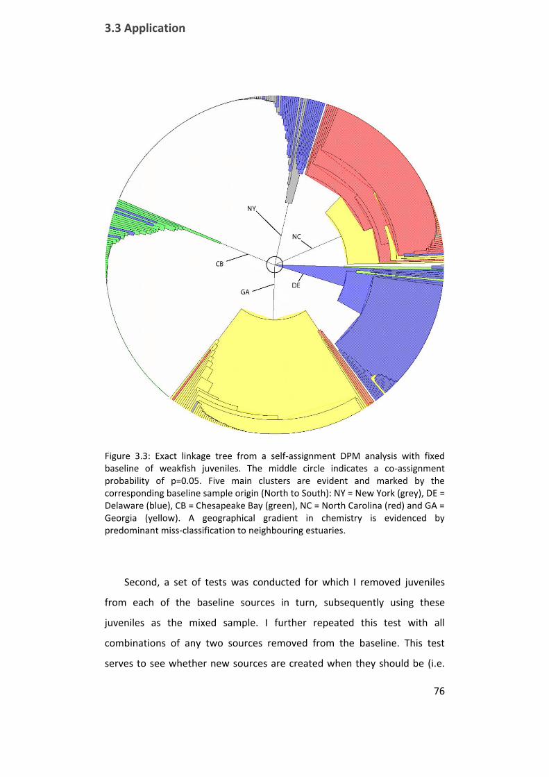
3.3 Application
76
Figure 3.3: Exact linkage tree from a self-assignment DPM analysis with fixed baseline of weakfish juveniles. The middle circle indicates a co-assignment probability of p=0.05. Five main clusters are evident and marked by the corresponding baseline sample origin (North to South): NY = New York (grey), DE = Delaware (blue), CB = Chesapeake Bay (green), NC = North Carolina (red) and GA = Georgia (yellow). A geographical gradient in chemistry is evidenced by predominant miss-classification to neighbouring estuaries.
Second, a set of tests was conducted for which I removed juveniles
from each of the baseline sources in turn, subsequently using these
juveniles as the mixed sample. I further repeated this test with all
combinations of any two sources removed from the baseline. This test
serves to see whether new sources are created when they should be (i.e.

Chapter 3. Bayesian mixture models for otolith geochemistry
77
when extra baseline sources are present in the dataset) and if the
corresponding individuals will associate with this extra-baseline source.
Lastly, I used this model to assign adult weakfish to natal sources, leaving
the possibility for extra-baseline sources. For these scenarios I used the
same prior as before, this time however I placed a Gamma(1,1) prior on k0k0.
Escobar & West (1995) noted that most often there will not be enough
information in the data to estimate this parameter – the inclusion of a
baseline however should provide some information about the scale of the
variance around the individual source means. Since information from the
baseline is now available, the baseline prior for the co-variance matrix was
now the mean within source covariance matrix.
The ‘cross-validation’ assignments of fish from a single source, with
that source omitted from the baseline, shows that the method works very
well for most sources (Table 3.2): the vast majority of fish are assigned to a
single extra-baseline source. DE is (not surprisingly) again the exception
with multiple predicted extra-baseline sources, two of which account for
most of the individuals due to the above mentioned multi-modality of that
source. The number of predicted sources is often slightly above the actual
number, highlighting the need to actually look at the number of fish within
each source to make statements about the number of contributing sources
(see also White et al. 2008). Results with combinations of two sources
omitted from the baseline show very similar patterns: most individuals are
assigned to mostly two distinct extra-baseline clusters (average proportion
p = 0:96p = 0:96, average modal number of predicted sources mode(K+) = 6:69mode(K+) = 6:69).
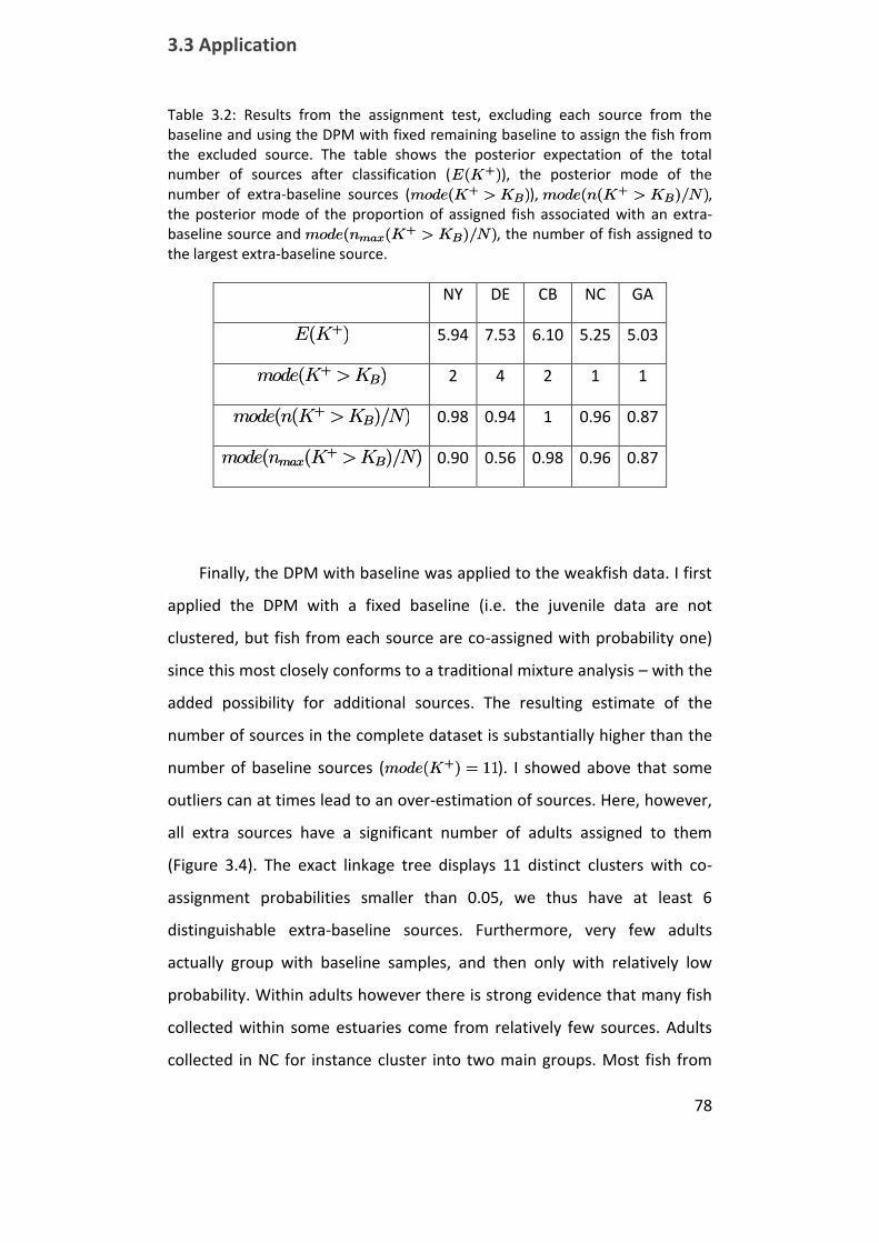
3.3 Application
78
Table 3.2: Results from the assignment test, excluding each source from the baseline and using the DPM with fixed remaining baseline to assign the fish from the excluded source. The table shows the posterior expectation of the total number of sources after classification (E(K+)E(K+)), the posterior mode of the number of extra-baseline sources (mode(K+ > KB)mode(K+ > KB)), mode(n(K+ > KB)=N)mode(n(K+ > KB)=N), the posterior mode of the proportion of assigned fish associated with an extra-baseline source and mode(nmax(K
+ > KB)=N)mode(nmax(K+ > KB)=N), the number of fish assigned to
the largest extra-baseline source.
Finally, the DPM with baseline was applied to the weakfish data. I first
applied the DPM with a fixed baseline (i.e. the juvenile data are not
clustered, but fish from each source are co-assigned with probability one)
since this most closely conforms to a traditional mixture analysis – with the
added possibility for additional sources. The resulting estimate of the
number of sources in the complete dataset is substantially higher than the
number of baseline sources (mode(K+) = 11mode(K+) = 11). I showed above that some
outliers can at times lead to an over-estimation of sources. Here, however,
all extra sources have a significant number of adults assigned to them
(Figure 3.4). The exact linkage tree displays 11 distinct clusters with co-
assignment probabilities smaller than 0.05, we thus have at least 6
distinguishable extra-baseline sources. Furthermore, very few adults
actually group with baseline samples, and then only with relatively low
probability. Within adults however there is strong evidence that many fish
collected within some estuaries come from relatively few sources. Adults
collected in NC for instance cluster into two main groups. Most fish from
NY DE CB NC GA
E(K+)E(K+) 5.94 7.53 6.10 5.25 5.03
mode(K+ >KB)mode(K+ >KB) 2 4 2 1 1
mode(n(K+ >KB)=N)mode(n(K+ >KB)=N) 0.98 0.94 1 0.96 0.87
mode(nmax(K+ >KB)=N)mode(nmax(K+ >KB)=N) 0.90 0.56 0.98 0.96 0.87

Chapter 3. Bayesian mixture models for otolith geochemistry
79
GA group as one large cluster, indicating that most adults found in this
estuary originate from a single source. The same holds for NY adults. CB
and DE adults however display only a slight amount of clustering and are
found in most extra-baseline source clusters, though the co-assignment
with fish in these clusters is usually low for fish from these estuaries.
Figure 3.4: Weakfish exact linkage tree from the DPM clustering model with fixed baseline. Sub-trees including adult weakfish are highlighted in light blue. Leaf colours indicate collection location (North to South): New York (grey), Delaware (blue), Chesapeake Bay (green), North Carolina (red) and Georgia (yellow).

3.3 Application
80
In the light of these results, I re-analysed the data, using the DPM for
clustering juvenile baseline samples together with adult samples (i.e. the
juvenile data is now not necessarily as separate source clusters). The
picture is decidedly less separated (Appendix A1): while there are still a
number of extra-baseline sources (mode(K+) = 10mode(K+) = 10), many fish also cluster
more closely with baseline samples from their estuary of collection,
supporting the homing hypothesis. This is particularly evident for NC fish,
although a large proportion of NC adults cluster on their own. Although not
particularly evident from the tree (due to overlap of labels to keep the tree
at a manageable size), some Chesapeake Bay samples also cluster within
baseline cluster predominated by NC juvenile signatures. Others from this
estuary cluster on their own with baseline fish from the same collection
location. Some Georgia adults are found with the corresponding baseline
signatures, while others cluster on their own. Fish also cluster with fish
from neighbouring estuaries on many occasions, but as shown above, this
may as well be due to miss-classification. Most strikingly, fish from DE and
NY often group together, both for adults and juveniles, but form separate
clusters for these age classes.
3.3.4 Classification with a (potentially) incomplete baseline
The DPM clustering results for the weakfish data (section 3.3.3)
demonstrate that there are likely extra-baseline sources present in the
adult dataset, which are distinct from those sampled for the baseline.
Thorrold et al. (1998) report that even within estuaries there are sufficient
differences in otolith signatures. Given that only a maximum of three
locations were sampled within each estuary, and given the catch statistics
for weakfish, one could assume that these extra-baseline sources are most
probably from other sites within any one or some of these estuaries. I
therefore applied the classification method for incomplete baselines to this
dataset, classifying adult fish to the, potentially incomplete, juvenile
baseline. Rather than keeping the baseline fixed, I clustered the baseline
Chapter 3. Bayesian mixture models for otolith geochemistry
81
with adult samples within each estuary since i) the pooled baseline within
each estuary seems to poorly represent the sampled locations (c.f. results
from the DPM with fixed baseline, section 3.3.3) and ii) this seems to reveal
more fine scale patterns.
First however, I validated the classification method with a set of tests.
To this end I added my own dataset (Neubauer et al. 2010) as a more
difficult and spatially hierarchical test set. In this dataset, I found
geographical variation of chemical signatures from hatchlings of common
triplefin (Forsterygion lapillum, Tripterygiidae) mainly between two main
islands and sites spread across these islands. A detailed study using this
classification method to assess connectivity between triplefin sub-
populations will be presented in Chapter 4, and I limit myself here to the
validation and illustration of the method’s features.
To assess whether the model performed its classification task in an
ideal situation in which the baseline is completely characterized, I
performed classification using self-assignment. Classification performance
was compared against the commonly used linear discriminant function
classification. To make sure that results were not dataset dependent, I
performed the same test on the weakfish baseline. I used fixed baselines
for the triplefin dataset because it allowed me to compare classification
success at the site specific scale against my earlier results. For the weakfish
data I clustered the baseline with the mixed sample within each region
because this seems to give more sensible results in the clustering
application and helps to demonstrate that the method works both ways.
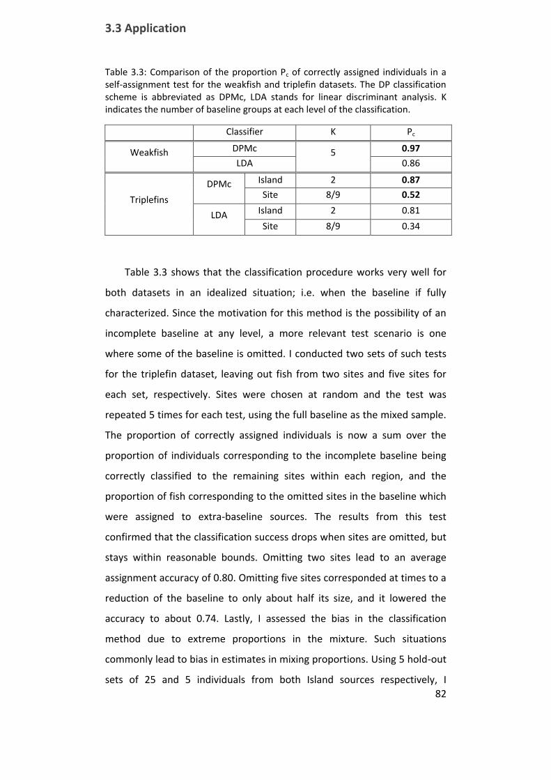
3.3 Application
82
Table 3.3: Comparison of the proportion Pc of correctly assigned individuals in a self-assignment test for the weakfish and triplefin datasets. The DP classification scheme is abbreviated as DPMc, LDA stands for linear discriminant analysis. K indicates the number of baseline groups at each level of the classification.
Classifier K Pc
Weakfish DPMc 5 0.97
LDA 0.86
Triplefins
DPMc Island 2 0.87
Site 8/9 0.52
LDA Island 2 0.81
Site 8/9 0.34
Table 3.3 shows that the classification procedure works very well for
both datasets in an idealized situation; i.e. when the baseline if fully
characterized. Since the motivation for this method is the possibility of an
incomplete baseline at any level, a more relevant test scenario is one
where some of the baseline is omitted. I conducted two sets of such tests
for the triplefin dataset, leaving out fish from two sites and five sites for
each set, respectively. Sites were chosen at random and the test was
repeated 5 times for each test, using the full baseline as the mixed sample.
The proportion of correctly assigned individuals is now a sum over the
proportion of individuals corresponding to the incomplete baseline being
correctly classified to the remaining sites within each region, and the
proportion of fish corresponding to the omitted sites in the baseline which
were assigned to extra-baseline sources. The results from this test
confirmed that the classification success drops when sites are omitted, but
stays within reasonable bounds. Omitting two sites lead to an average
assignment accuracy of 0.80. Omitting five sites corresponded at times to a
reduction of the baseline to only about half its size, and it lowered the
accuracy to about 0.74. Lastly, I assessed the bias in the classification
method due to extreme proportions in the mixture. Such situations
commonly lead to bias in estimates in mixing proportions. Using 5 hold-out
sets of 25 and 5 individuals from both Island sources respectively, I
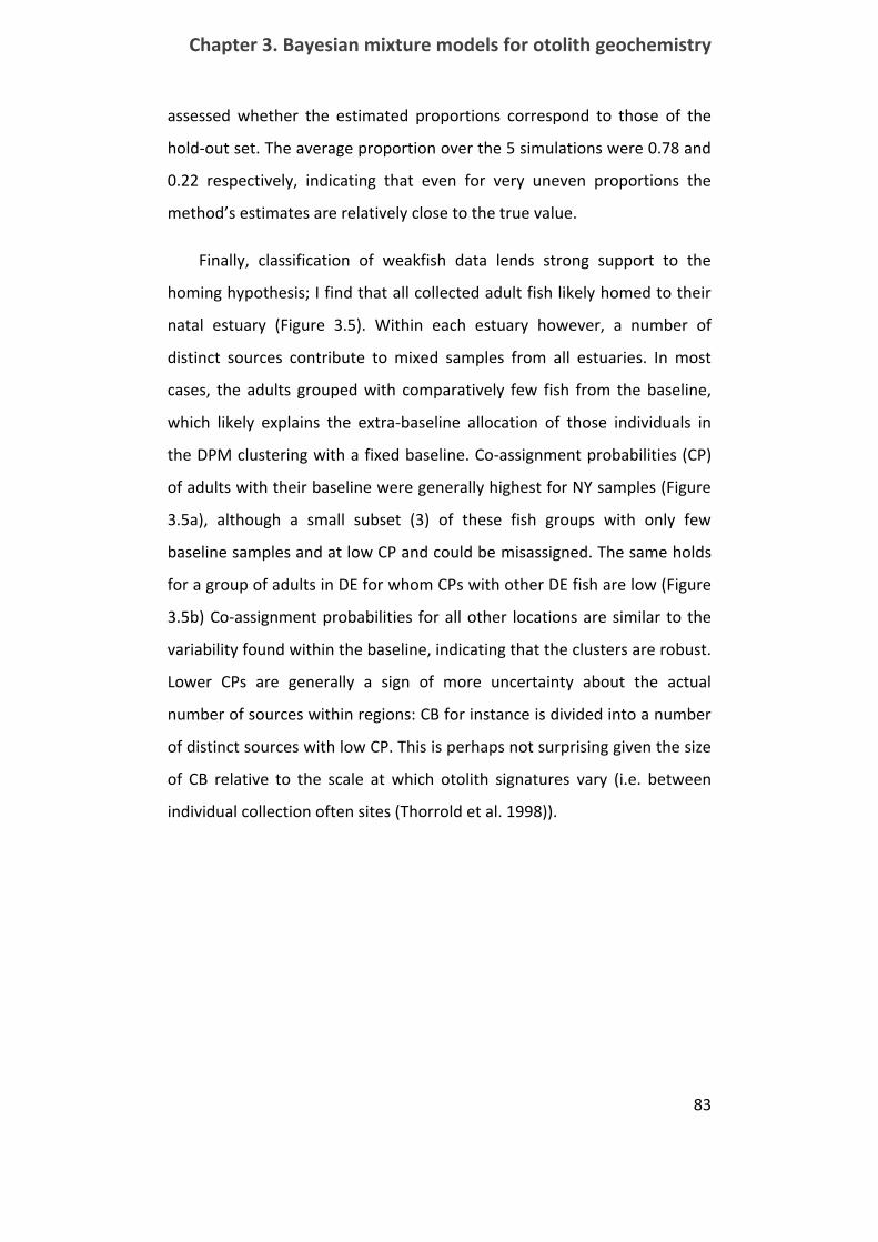
Chapter 3. Bayesian mixture models for otolith geochemistry
83
assessed whether the estimated proportions correspond to those of the
hold-out set. The average proportion over the 5 simulations were 0.78 and
0.22 respectively, indicating that even for very uneven proportions the
method’s estimates are relatively close to the true value.
Finally, classification of weakfish data lends strong support to the
homing hypothesis; I find that all collected adult fish likely homed to their
natal estuary (Figure 3.5). Within each estuary however, a number of
distinct sources contribute to mixed samples from all estuaries. In most
cases, the adults grouped with comparatively few fish from the baseline,
which likely explains the extra-baseline allocation of those individuals in
the DPM clustering with a fixed baseline. Co-assignment probabilities (CP)
of adults with their baseline were generally highest for NY samples (Figure
3.5a), although a small subset (3) of these fish groups with only few
baseline samples and at low CP and could be misassigned. The same holds
for a group of adults in DE for whom CPs with other DE fish are low (Figure
3.5b) Co-assignment probabilities for all other locations are similar to the
variability found within the baseline, indicating that the clusters are robust.
Lower CPs are generally a sign of more uncertainty about the actual
number of sources within regions: CB for instance is divided into a number
of distinct sources with low CP. This is perhaps not surprising given the size
of CB relative to the scale at which otolith signatures vary (i.e. between
individual collection often sites (Thorrold et al. 1998)).
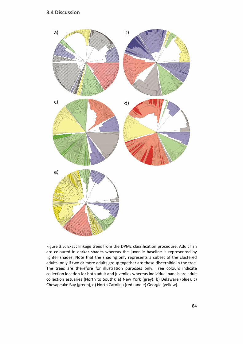
3.4 Discussion
84
Figure 3.5: Exact linkage trees from the DPMc classification procedure. Adult fish are coloured in darker shades whereas the juvenile baseline is represented by lighter shades. Note that the shading only represents a subset of the clustered adults: only if two or more adults group together are these discernible in the tree. The trees are therefore for illustration purposes only. Tree colours indicate collection location for both adult and juveniles whereas individual panels are adult collection estuaries (North to South): a) New York (grey), b) Delaware (blue), c) Chesapeake Bay (green), d) North Carolina (red) and e) Georgia (yellow).
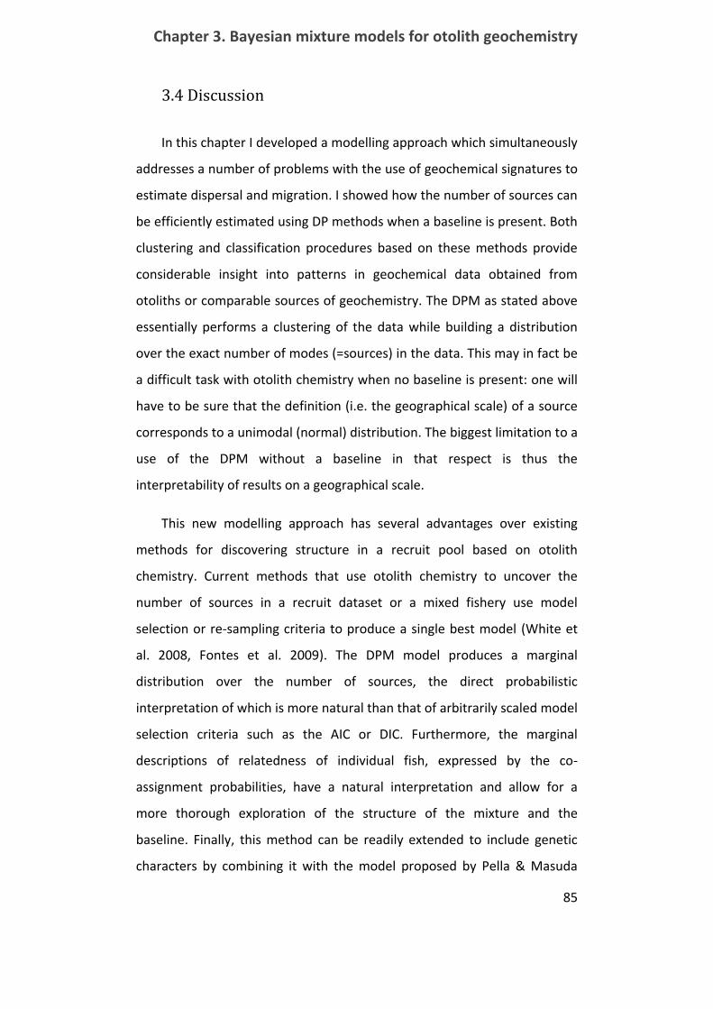
Chapter 3. Bayesian mixture models for otolith geochemistry
85
3.4 Discussion
In this chapter I developed a modelling approach which simultaneously
addresses a number of problems with the use of geochemical signatures to
estimate dispersal and migration. I showed how the number of sources can
be efficiently estimated using DP methods when a baseline is present. Both
clustering and classification procedures based on these methods provide
considerable insight into patterns in geochemical data obtained from
otoliths or comparable sources of geochemistry. The DPM as stated above
essentially performs a clustering of the data while building a distribution
over the exact number of modes (=sources) in the data. This may in fact be
a difficult task with otolith chemistry when no baseline is present: one will
have to be sure that the definition (i.e. the geographical scale) of a source
corresponds to a unimodal (normal) distribution. The biggest limitation to a
use of the DPM without a baseline in that respect is thus the
interpretability of results on a geographical scale.
This new modelling approach has several advantages over existing
methods for discovering structure in a recruit pool based on otolith
chemistry. Current methods that use otolith chemistry to uncover the
number of sources in a recruit dataset or a mixed fishery use model
selection or re‐sampling criteria to produce a single best model (White et
al. 2008, Fontes et al. 2009). The DPM model produces a marginal
distribution over the number of sources, the direct probabilistic
interpretation of which is more natural than that of arbitrarily scaled model
selection criteria such as the AIC or DIC. Furthermore, the marginal
descriptions of relatedness of individual fish, expressed by the co-
assignment probabilities, have a natural interpretation and allow for a
more thorough exploration of the structure of the mixture and the
baseline. Finally, this method can be readily extended to include genetic
characters by combining it with the model proposed by Pella & Masuda
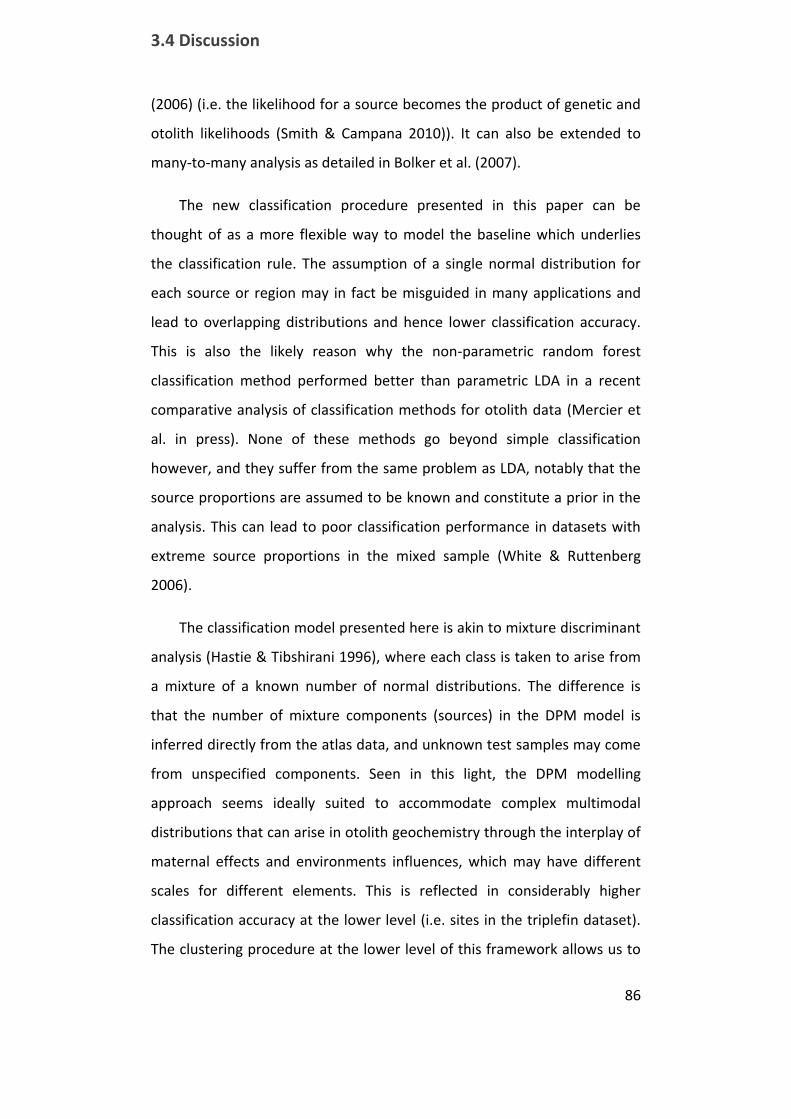
3.4 Discussion
86
(2006) (i.e. the likelihood for a source becomes the product of genetic and
otolith likelihoods (Smith & Campana 2010)). It can also be extended to
many-to-many analysis as detailed in Bolker et al. (2007).
The new classification procedure presented in this paper can be
thought of as a more flexible way to model the baseline which underlies
the classification rule. The assumption of a single normal distribution for
each source or region may in fact be misguided in many applications and
lead to overlapping distributions and hence lower classification accuracy.
This is also the likely reason why the non-parametric random forest
classification method performed better than parametric LDA in a recent
comparative analysis of classification methods for otolith data (Mercier et
al. in press). None of these methods go beyond simple classification
however, and they suffer from the same problem as LDA, notably that the
source proportions are assumed to be known and constitute a prior in the
analysis. This can lead to poor classification performance in datasets with
extreme source proportions in the mixed sample (White & Ruttenberg
2006).
The classification model presented here is akin to mixture discriminant
analysis (Hastie & Tibshirani 1996), where each class is taken to arise from
a mixture of a known number of normal distributions. The difference is
that the number of mixture components (sources) in the DPM model is
inferred directly from the atlas data, and unknown test samples may come
from unspecified components. Seen in this light, the DPM modelling
approach seems ideally suited to accommodate complex multimodal
distributions that can arise in otolith geochemistry through the interplay of
maternal effects and environments influences, which may have different
scales for different elements. This is reflected in considerably higher
classification accuracy at the lower level (i.e. sites in the triplefin dataset).
The clustering procedure at the lower level of this framework allows us to
Chapter 3. Bayesian mixture models for otolith geochemistry
87
cluster without a priori division into sites, which provides a method to
assess whether the clustering is clear cut or poorly resolved at smaller
spatial scales. The possibility for recruits to come from un‐sampled sites
make the DPM and DPMc approach an excellent tool for exploring
connectivity based on geochemical tracers in geographically and chemically
complex landscapes. It is thus a more realistic procedure in most otolith
applications in the marine environment where the assumption of a
complete baseline can rarely be justified.
Classification of the weakfish data confirmed the suspicion from the
self-assignment test with the DPM cluster model: I found that classification
to neighbouring estuaries reported in earlier studies was likely due to
misclassification and that natal homing is likely near perfect. The genetic
homogeneity of the stock indicates that some dispersal between estuaries
must happen, but since very few migrants per generation are enough to
maintain a genetically homogenous population, this number could be next
to undetectable with manageable sample sizes for otolith geochemistry.
One alternative explanation for the perfect homing pattern observed
here is that many adult weakfish signatures are sufficiently different from
the bulk of the baseline signatures. Given that allocation to any of the
baseline estuaries would then be equally unlikely, the classification would
be driven by the allocation of a few individuals to a baseline sample, which
would influence the estimates of mixing proportions which in turn
dominate the likelihood for any estuary. In simpler terms: if the model is
very uncertain about where some adults may have come from, then these
fish are more likely to be assigned to the region to which most other fish
have already been assigned. This would seem like a likely explanation in
the light of results from the DPM clustering model with fixed baseline:
most adults cluster together and apart from the baseline. Allowing the
baseline to be clustered with adults however shows that this may be an
3.4 Discussion
88
artefact of pooling sites within estuaries, and that many adults cluster as
closely with the baseline as they do amongst themselves. For DE and NY
many adults cluster together and apart from juveniles, but this is not a
generality. The classification trees confirm this: adults usually cluster with
the baseline in a number of distinct clusters and with comparable CP to
those seen between baseline samples. The exception may be a relatively
large group of adults in DE and a small group from NY for which CP with
their baseline were relatively low.
All models developed in this chapter could be applied to other types of
geochemical tracers, such as stable isotopes, as well as related techniques
using other calcified structures or even soft tissue trace elements. The
approach presented here is a general Bayesian (fuzzy) clustering and
classification framework which may even be applied to unrelated problems
for which clustering based on probabilistic assumptions seems
advantageous. In this respect the model and hierarchical tree building
method employed here is related to Bayesian hierarchical clustering (Heller
& Ghahramani 2005), which aims to directly construct a hierarchical
clustering tree from data based on the same probabilistic assumptions. The
node height in Bayesian hierarchical clustering is however not directly
interpretable in probabilistic terms ‐ a feature which seems a clear
advantage of the present framework. In conclusion, this chapter develops
flexible and useful methods to be used with otolith chemical signatures. It
is shown to perform well – especially with regard to estimating missing
sources in the baseline dataset, which up until now had been a significant
limit for the use of otolith geochemistry in complex environments. The
DPM methods therefore provide a considerable step towards a more
general applicability of geochemistry for questions of dispersal and
migration.
89
CHAPTER 4
4. Larval dispersal pathways in a reef fish
metapopulation: Contrasting empirical and
simulation measures
4.1 Introduction
Dispersal of propagules and adults in fragmented animal populations
(metapopulations) is a major determinant of population dynamics (Hanski
1999, Kendall et al. 2000, Gaines et al. 2007, Gouhier et al. 2010). The
spatial configuration of populations and their ensuing connectivity will
further determine the persistence of local populations and the viability of
the metapopulation network as a whole (Hastings & Botsford 2006, Artzy-
Randrup & Stone 2010). Connectivity measures are therefore vital for
resource management (Fogarty & Botsford 2007) as well as conservation
planning (Crooks & Sanjayan 2006).
In the marine environment, dispersal of larvae between local
populations can link dynamics of marine populations and communities
over large geographical scales (Gaines et al. 2007, Gouhier et al. 2010).
While the importance of connections has been much discussed in theory
(Armsworth 2002, Hastings & Botsford 2006, Gouhier et al. 2010) and in
the light of conservation questions (Botsford et al. 2001, Guichard et al.
2004, Baskett et al. 2007), empirical estimates of connectivity in marine
4.1 Introduction
90
metapopulations have been difficult to obtain (Cowen et al. 2007). As a
result, limited information about dispersal patterns has contributed to
uncertainties in spatial management of marine resources and the optimal
implementation of marine reserves and reserve networks (Sale et al. 2005,
Halpern et al. 2006). Unless we obtain reliable estimates of demographic
connectivity in marine communities, we cannot predict whether reserves
or spatial management actions will serve their desired purpose (Stobutzki
2001).
Many studies emphasize the importance of local hydrodynamics in
deciding dispersal outcomes and their demographic consequences (Black &
Moran 1991, Guichard et al. 2001, Gilg & Hilbish 2003, Byers & Pringle
2006, Swearer & Shima 2010, White et al. 2010). In particular, variability
and heterogeneity in flow fields are not only responsible for spatially
heterogeneous connectivity (Mace & Morgan 2006, Mitarai et al. 2008,
Siegel et al. 2008, White et al. 2010), they also provide a means for
population maintenance in directional (advective) flows (Largier 2003,
Byers & Pringle 2006). Given these results, variability in flow may actually
be as important a determinant of population structure and connectivity as
mean flow patterns.
Specifically, marine organisms are predicted to adapt to exploit such
heterogeneities (Byers & Pringle 2006) and many larvae indeed show
species-specific patterns of utilizing spatially heterogeneous flow
(Breitburg et al. 1995, Paris & Cowen 2004, Morgan & Fisher 2010). In the
face of such potential adaptations, it will be difficult to make specific
predictions about dispersal patterns from hydrodynamic models alone.
Such models are important for developing hypotheses about potential
dispersal pathways, especially when paired with species-specific
behavioural information (Paris & Cowen 2004, Koehl et al. 2007, Leis 2007).
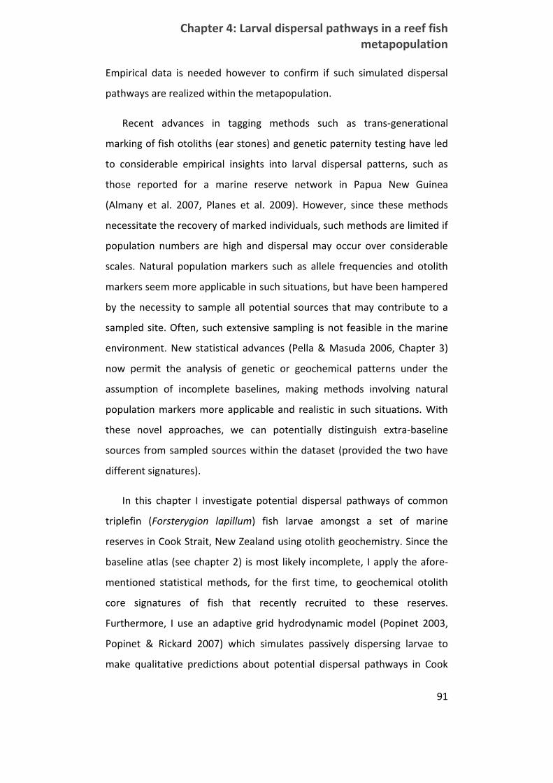
Chapter 4: Larval dispersal pathways in a reef fish metapopulation
91
Empirical data is needed however to confirm if such simulated dispersal
pathways are realized within the metapopulation.
Recent advances in tagging methods such as trans-generational
marking of fish otoliths (ear stones) and genetic paternity testing have led
to considerable empirical insights into larval dispersal patterns, such as
those reported for a marine reserve network in Papua New Guinea
(Almany et al. 2007, Planes et al. 2009). However, since these methods
necessitate the recovery of marked individuals, such methods are limited if
population numbers are high and dispersal may occur over considerable
scales. Natural population markers such as allele frequencies and otolith
markers seem more applicable in such situations, but have been hampered
by the necessity to sample all potential sources that may contribute to a
sampled site. Often, such extensive sampling is not feasible in the marine
environment. New statistical advances (Pella & Masuda 2006, Chapter 3)
now permit the analysis of genetic or geochemical patterns under the
assumption of incomplete baselines, making methods involving natural
population markers more applicable and realistic in such situations. With
these novel approaches, we can potentially distinguish extra-baseline
sources from sampled sources within the dataset (provided the two have
different signatures).
In this chapter I investigate potential dispersal pathways of common
triplefin (Forsterygion lapillum) fish larvae amongst a set of marine
reserves in Cook Strait, New Zealand using otolith geochemistry. Since the
baseline atlas (see chapter 2) is most likely incomplete, I apply the afore-
mentioned statistical methods, for the first time, to geochemical otolith
core signatures of fish that recently recruited to these reserves.
Furthermore, I use an adaptive grid hydrodynamic model (Popinet 2003,
Popinet & Rickard 2007) which simulates passively dispersing larvae to
make qualitative predictions about potential dispersal pathways in Cook

4.2 Methods
92
Strait, New Zealand. The grid refinement of the model is adaptive and
dynamic, which makes it particularly suitable for modelling in areas of
complex flow where fixed grid approximations may be impractical due to
implement due to very high computational requirements at a reasonable
resolution. To gain insight into realized dispersal pathways and potential
mechanisms of connectivity in this system, predictions from the simulation
model are then compared with empirically inferred dispersal events.
4.2 Methods
4.2.1 Study system and otolith core chemistry atlas
I established a reference atlas of hatchling (core) otolith signatures
from 17 sites around Cook Strait, New Zealand (Figure 4.1) by sampling
otoliths of newly hatched larvae of the common triplefin (Forsterygion
lapillum), a reef fish that is commonly found in sheltered shallow reefs
around New Zealand (Clements 2003, Feary & Clements 2006). Its relatively
long larval duration of ~52 days (Shima & Swearer 2009a) makes it a good
candidate to study dispersal in marine metapopulations. Our collection
sites for the reference atlas are distributed hierarchically across multiple
regions on either side of Cook Strait, which separates the two main Islands
of New Zealand (Figure 4.1). Further details about analytical methods, the
atlas and the study species can be found in Chapter 2.
4.2.2 Recruit otolith preparation and pre‐processing
Between 50 and 62 days after collecting hatchlings from the
aforementioned sites, I collected a total of 169 recruits of F. lapillum in
three marine reserves around Cook Strait, New Zealand (Figure 4.1),
namely at Taputearanga Marine Reserve in Wellington (60 recruits), Long
Island Marine Reserve, Queen Charlotte Sound (59 recruits) and Kapiti
Island, upstream of Cook Strait (40 recruits).
Chapter 4: Larval dispersal pathways in a reef fish metapopulation
93
Figure 4.1 : a) Map of Cook Strait, New Zealand and b) the sampling domain. Our 17 baseline sampling sites (grey circles) are scattered either side of Cook Strait. Black outlines mark borders of regional marine reserves where recruits were collected (arrows on blow-up aerial photographs).
Taputearanga marine reserve in Wellington is located on the southern
coast of the city of Wellington, at proximity to the opening of Wellington
Harbour (Figure 4.1). Wellington’s south coast is characterized by its
exposure to southerly swells which batter the coast throughout the year.
Local populations of breeding F. lapillum are found in this reserve only in a
few sites which are sheltered from swell by Taputeranga Island, a small
island about 50m offshore in Island Bay, Wellington.
Kapiti Island and its associated marine reserve are located ~50km north
of Wellington and approximately 5.6km offshore (Figure 4.1). Bathed in
waters of the D’Urville current which pushes water south‐eastward
through Cook Strait (Heath 1986, Chiswell & Stevens). F. lapillum breeds in

4.2 Methods
94
the relatively sheltered eastern waters of the Island, at isolated sites that
are free from otherwise ubiquitous brown algae.
Long Island reserve is located in the opening of Queen Charlotte Sound
in the Marlborough Sounds on the upper South Island of New Zealand
(Figure 4.1). Little swell reaches this island, however, strong tidal currents
and strong northerly wind‐chop restrict breeding sites for my study species
to very few small patches close to the shores of the island.
Immediately after collection these recruits were placed in vials
containing 95%95% analytical grade ethanol. All otolith handling material was
rinsed in weak acid for 24h before being used in the otolith preparation
procedure. Saggital otoliths were extracted using plastic tweezers and
were subsequently placed into well plates for handling. Extractions and
handling took place in an ultra-clean positive pressure laboratory and
under a class 100 laminar flow hood. After extraction, the otoliths were
subjected to two consecutive rinsing baths in 15%15% NaOH buffered hydrogen
peroxide solution for 24h each. Between and after each cleaning bath the
otoliths were cleaned three times with pure (18.2 MÐÐ) water. Air‐dried
otoliths were then mounted onto circular slides using chemically inert
epoxy resin (Buehler Epothin; Buehler, Lake Bluff, Illinois, USA). Each
otolith was polished to the core using 9¹¹m diamond lapping film (3M)
mounted on an 8 inch (20 cm) lapping wheel (Model 920; South Bay
Technologies, San Clemente, California, USA) and again cleaned as
described above following the polishing.
Chemical analysis of recruit otoliths followed methods described in
(Shima & Swearer 2009a). Briefly, I used Laser Ablation Inductively Coupled
Mass Spectrometry (LA‐ICPMS) to sample material corresponding to the
core of recruits by ablating in a deepening pit using a 25¹¹m laser spot. A
spike in 5555Mn served as an indicator of core material (Brophy et al. 2004,
Ruttenberg et al. 2005). A significant number of otoliths had to be
Chapter 4: Larval dispersal pathways in a reef fish metapopulation
95
discarded as these were either damaged, ground too far down below the
core, or we failed to locate the otolith core in the recruit. A total of 69
samples remained for final analysis ‐ 29 from Wellington’s Marine reserve,
20 from Long Island Marine Reserve and 20 from Kapiti. Following the
protocol for the hatchling atlas (see chapter 2), I averaged ten scans across
this peak to obtain the natal signature.
4.2.3 Selecting elements for analysis of otolith cores
In order to ensure that the data I collected from the recruits is
comparable to signatures from the reference atlas, I treated the mean and
variance of log-transformed elemental distributions in the atlas samples as
coming from a normal distribution of unknown characteristics. I then
estimated these characteristics (mean and variance) using Bayesian
inference. For background on Bayesian statistics and reasoning the reader
is referred to Gelman (2003). Briefly, Bayesian statistics employ Bayes
theorem for statistical inference. In particular, the Bayesian approach
defines that the posterior distribution of unknown parameters given the
data is proportional to the likelihood of the data times the prior
distribution for the parameters (see also Chapter 1). The prior specifies a
distribution which reflects our prior knowledge about model parameters. It
can be shown that the posterior distribution is a weighted average of the
information in the data at hand and the prior knowledge, where the weight
of each is determined by their relative precision. Vague (or diffuse) priors
(with large variance and hence very little weight) can be used when we
have little or no information about the range of parameters to be
estimated.
To encode the absence of prior knowledge about the distribution of
signatures from the reference atlas, I placed a vague Gamma(10¡610¡6,10¡610¡6)
prior on the precision and a vague normal prior N(0,1000) on the mean of
the elemental distribution of all measured elements. I retained elements

4.2 Methods
96
for which > 95%> 95% of recruit observations fell within the 95% credible
interval of the estimated posterior distribution for each element. This
analysis was performed using the WinBUGS (Lunn et al. 2000) software for
Bayesian computation.
4.2.4 Statistical analysis of otolith chemistry
While my baseline sampling of potential natal sources covers most
areas with significant local triplefin populations in Cook Strait (Smith 2008),
it almost certainly does not cover all spawning sites. I therefore use the
Dirichlet mixture classification model (DPMc, developed in chapter 3,
section 3.2.3) to assign fish to natal origins. Using cross-validation on the
baseline samples, I reported reasonable assignment success when
classifying individuals to one of the two major New Zealand islands in Cook
Strait (North vs. South island) (see chapter 2). For the purpose of this
chapter I was interested in a more resolved picture. Therefore, I repeated
the cross-validation tests (described in chapter 3) at the scale of regions
within Cook Strait, as defined in chapter 2. In that chapter I found that
regions were not significantly different, however the weak separation may
have been due to grouping sites of very different characteristics into
arbitrary regions.
Given that regions can be reasonably discerned with the DPMc (see
Results), I classified fish to regions within Cook Strait, keeping the baseline
sites as fixed entities (i.e. they are clustered with co-assignment probability
p = 1p = 1) as for the test examples in chapter 3. In fact, I found in preliminary
studies that clustering the baseline at the site level for this dataset often
produced a great number of clusters, probably due to the strong clutch
effect which outweighs any geographical pattern. Furthermore, this large
number of clusters leads to extremely slow convergence of the Gibbs
sampler. Thus, keeping the sites as fixed entities ensures that results
remain interpretable at this level.
Chapter 4: Larval dispersal pathways in a reef fish metapopulation
97
To characterize classification probabilities, I used both posterior
probabilities for regions, as well as posterior entropy, measured as the
information entropy of the expectations of posterior assignment
probabilities ÁÁ over all KK possible regions. The entropy is defined as
H[Ái] =¡PK
k=1Ái;k logÁi;kH[Ái] =¡PK
k=1Ái;k logÁi;k
where Ái =PS
s=1 p(³i;s = kjµ)Ái =PS
s=1 p(³i;s = kjµ) , the approximated expected value of
p(³i = kjµ)p(³i = kjµ) from S draws by Markov Chain Monte Carlo from this
distribution. The information entropy measures the uniformity of a
distribution: if the predictive distribution predicts every source k with the
same probability, this entropy is maximized with value Hmax = logKHmax = logK. Vice
versa, if the prediction is without uncertainty, the entropy will be zero.
Dividing by HmaxHmax produces a measure of evenness E = H=HmaxE = H=Hmax between
zero and one. The posterior entropy thus provides a single measure to
quantify the uncertainty in the classifications produced by DPMc. Lastly,
clustering within each site is visualized using trees generated from marginal
co-assignment probabilities to source clusters (see chapter 3, section
3.2.4), where the branch length of the trees is a direct measure of the
probability that two fish originate from the same water-mass.
4.2.5 Simulation models of dispersal
I conducted two distinct simulation experiments using the Gerris flow
solver, an adaptive mesh simulation model that solves the Boussinesq
incompressible hydrostatic equations of ocean dynamics by making a
‘shallow water’ approximation which neglects the vertical coupling terms
(Popinet 2003, Popinet & Rickard 2007). This depth integrated model
allows features of interest, such as eddies developing along the complex
coastline of Cook Strait, to be adaptively resolved to a user specified
resolution. Since the refinement is adaptive with respect to such specified
features only, this resolution can be set to high values without the
exponential increase in computational requirements usually found in fixed
4.2 Methods
98
grid models. Mesh refinement was chosen to refine to a maximum
resolution of 117.19m. The coastline was modelled with the same
resolution, which was kept fixed for the topography.
A version of the Gerris ocean model has recently been applied to
oceanographic modelling of tidal cycles in Cook Strait (Msadek 2005) and
the present simulations are extensions of this work. The model domain
includes Cook Strait as well as the Taranaki Bight and Tasman Bay to the
west and Palliser Bay to the east. Msadek’s (2005) work only included tidal
forcing and neglected barotropic flow or any forcing due to wind. The
present simulation contains forcing by wind fields, corresponding to the
time of our empirical investigations. These were obtained from the NZLAM
model (National Institute of Water and Atmospheric Research, New
Zealand) at a resolution of 15km. A hyperbolic-tangent shaped gradient in
sea surface height (SSH) was imposed to approximate observed differences
between the Tasman Sea and the Pacific Ocean. The boundaries of the
model domain were forced by SSH and current velocity values
corresponding to the larval period of collected recruits, obtained from a
wind driven NZ wide Regional Ocean Model (ROMS). The model was
initiated on Jan 1st 2008 and ran for 52days. A separate manuscript
describing model validation against drifters and acoustic Doppler current
profiler data as well as a comparison to outputs from a ROMS model of the
same region is in preparation and will be presented elsewhere (Neubauer
et al. in prep).
I released passive tracers at locations and in densities which
approximate those predicted by a model-generated distribution map of F.
lapillum (Smith 2008). Release locations are between 3-10m in depth and
confined to predefined squares within each region of interest (i.e. locations
with significant abundance of F. lapillum within Wellington, Marlborough
Sounds and Kapiti regions). Although F. lapillum can be found throughout
Chapter 4: Larval dispersal pathways in a reef fish metapopulation
99
NZ, it appears to be most abundant in sheltered regions of the Cook Strait,
especially around Wellington and within the Marlborough Sounds. The
model predicts little to no significant abundance of F. lapillum upstream of
Cook Strait (i.e. north of Kapiti and west of the Marlborough Sounds as well
as on the exposed eastern and western side of the northern South Island).
This information was consistent with my own personal observations of
common triplefin distribution in the Cook Strait region. I therefore assume
that little, if any, dispersal into Cook Strait happens on an ecologically
relevant timescale. Virtual larvae were released over a two week window
starting on day 3 of the simulation. The simulation model outputs are
employed to describe the movements of tracers in a qualitative way, in
order to make hypotheses about potential dispersal pathways and
mechanisms. These are then compared to dispersal routes predicted by
otolith chemistry. A more detailed description of the Gerris ocean model
including a detailed application of this model to simulations of larval
dispersal will be given elsewhere.
4.3 Results
4.3.1 Results from otolith microchemistry
Detection limits and consistency standards for all measured elements
are given in table 1. Most elements were above the detection limit for the
majority of samples, however, S, Mn, Cu, Zn and Pb were below detection
limits for some fish. Comparison between the predictive distribution of
baseline samples and sampled recruit cores revealed that Mg and Mn were
significantly higher in hatchling cores than in recruit cores (Figure 4.2).
These two elements were thus omitted from subsequent analyses (see the
‘Discussion’ section on maternal effects).
The hierarchical organization in the DPMc classification model
developed in Chapter 3 improves classification success on the regional
4.3 Results
100
scale to almost twice that of the linear discriminant analysis (LDA) used in
chapter 2. Five cross-validation studies with 40 fish found an average
accuracy of 67.6% from this method as compared to 34.9% mean accuracy
with LDA.
I found distinct dispersal signatures in both the North and South Island
recruits. Overall, associations at the site level as revealed by the exact
linkage algorithm were rather low in terms of co-assignment probabilities
with existing sites, indicating that either assignment to these sites is
relatively uncertain and/or extra-baseline sites may often be present.
Assignments at the regional level had mostly high posterior probabilities,
although some ambiguous cases can also be found (Figure 4.3).
North Island recruits probably originated at both Wellington and Kapiti
Island for both of these sites, indicating that connections exist in both
directions (Figure 4.3a-d). Expectations of posterior assignment
probabilities were usually lower for Kapiti Island than those for Wellington,
indicating that there is some degree of overlap with other regions. Slightly
more recruits to Kapiti Island marine reserve seemed to have come from
Wellington and visa-versa, indicating that dispersal on that scale is rather
common.
Recruits collected from Kapiti are grouped into two distinct clusters for
each source region at the site level, indicating that multiple sites contribute
to the recruit pool in the Kapiti marine reserve (Figure 4.3a-b). All clusters
are associated with a baseline site: the larger cluster from Wellington is
most closely associated with Wellington Harbour baseline signatures, while
the smaller cluster is closest in similarity to Wellington coastal signatures.
Most Kapiti sourced recruits associate with Northern Kapiti sites, from both
within and outside the Kapiti marine reserve.

Chapter 4: Larval dispersal pathways in a reef fish metapopulation
101
Table 4.1: Distribution of trace element concentrations (in mol per mol Ca; note multiplier for each element column) relative to detection limits. Given are elemental concentrations for the quantiles that bracket 95% of all observations made from sampled otoliths, and the median value. Detection limits (DL in mol per mol Ca) and external precision estimates (consistency standard, CS) for analyses of hatchling otoliths by LA-ICP-MS. DL estimates based on 20 blank analyses. Estimates of external precision are given in relative standard deviations (%RSD) and are based on 11 blocks of samples (a block is a series of samples bracketed by standards), treating the NIST (National Institute of Standards and Technology) standard that is just below the standard used for calibration for each element as unknown and calculating the Element:Ca ratio for this standard for each block of samples.
Element Sample quantiles DL CS NIST(CS)
0.025 0.5 0.975
7Li7Li (¤10¡6)(¤10¡6) 5.56 11.01 23.48 21.68 8.54 614
11B11B (¤10¡3)(¤10¡3) 0.092 0.16 0.20 0.062 9.14 614
24Mg24Mg (¤10¡3)(¤10¡3) 0.11 0.25 0.53 0.021 7.83 612
31P31P (¤10¡3)(¤10¡3) 0.60 1.17 4.01 0.14 13.27 612
34S34S (¤10¡3)(¤10¡3) 0.28 0.60 1.21 0.43 6.16 612
55Mn55Mn (¤10¡6)(¤10¡6) 2.66 23.25 266.69 6.59 7.32 612
63Cu63Cu (¤10¡6)(¤10¡6) 0 0.50 1.36 3.57 8.37 614
66Zn66Zn (¤10¡6)(¤10¡6) 0 5.70 58.66 6.76 8.26 614
88Sr88Sr (¤10¡3)(¤10¡3) 1.87 2.50 3.77 0.00093 7.48 612
138Ba138Ba (¤10¡6)(¤10¡6) 1.92 13.15 56.08 0.088 7.77 614
208Pb208Pb (¤10¡6)(¤10¡6) 0 0.048 1.97 0.16 7.21 614
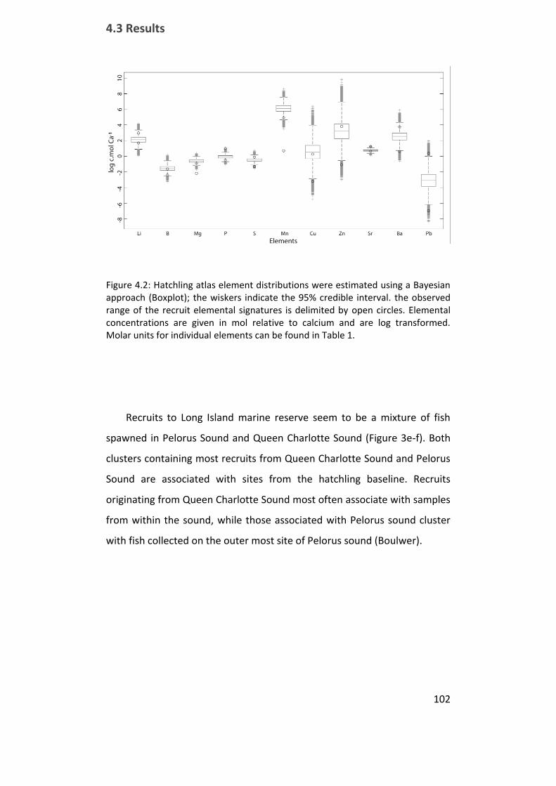
4.3 Results
102
Figure 4.2: Hatchling atlas element distributions were estimated using a Bayesian approach (Boxplot); the wiskers indicate the 95% credible interval. the observed range of the recruit elemental signatures is delimited by open circles. Elemental concentrations are given in mol relative to calcium and are log transformed. Molar units for individual elements can be found in Table 1.
Recruits to Long Island marine reserve seem to be a mixture of fish
spawned in Pelorus Sound and Queen Charlotte Sound (Figure 3e-f). Both
clusters containing most recruits from Queen Charlotte Sound and Pelorus
Sound are associated with sites from the hatchling baseline. Recruits
originating from Queen Charlotte Sound most often associate with samples
from within the sound, while those associated with Pelorus sound cluster
with fish collected on the outer most site of Pelorus sound (Boulwer).
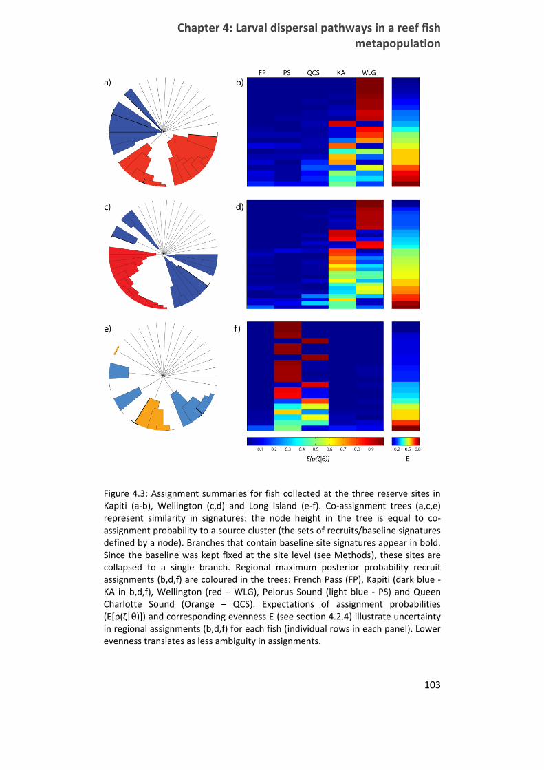
Chapter 4: Larval dispersal pathways in a reef fish metapopulation
103
Figure 4.3: Assignment summaries for fish collected at the three reserve sites in Kapiti (a-b), Wellington (c,d) and Long Island (e-f). Co-assignment trees (a,c,e) represent similarity in signatures: the node height in the tree is equal to co-assignment probability to a source cluster (the sets of recruits/baseline signatures defined by a node). Branches that contain baseline site signatures appear in bold. Since the baseline was kept fixed at the site level (see Methods), these sites are collapsed to a single branch. Regional maximum posterior probability recruit assignments (b,d,f) are coloured in the trees: French Pass (FP), Kapiti (dark blue - KA in b,d,f), Wellington (red – WLG), Pelorus Sound (light blue - PS) and Queen Charlotte Sound (Orange – QCS). Expectations of assignment probabilities (E[p(ζ|θ)]) and corresponding evenness E (see section 4.2.4) illustrate uncertainty in regional assignments (b,d,f) for each fish (individual rows in each panel). Lower evenness translates as less ambiguity in assignments.

4.3 Results
104
Figure 4.4: Comparison of log transformed signatures from samples in the isolated cluster of Wellington sourced recruits vs. all other recruits assigned to Wellington (in c.mol per mol of calcium, for multipliers see table 1). Remaining samples are represented by minimum and maximum values (open circles), samples from the cluster in question are represented by the box plot.
4.3.2 Results from hydrodynamic simulation experiments
The hydrodynamic model for Cook Strait predicts significant
downstream dispersal as well as some nearshore upstream dispersal in
Cook Strait (Figures 4.5-4.8). The dispersal pathways obtained from these
simulations were similar across cohorts released over a two week window
owing to strong mean currents and a long larval duration, and Figure 4.5-
4.8 show results from a representative cohort. Tracers released in Kapiti
move quickly downstream, though some seem to be naturally retained
inshore (Figure 4.5). Tracers initially move towards the Kapiti coast (Figure
4.5b), where a number of these tracers get retained near the coast for the
extent of the simulations. Others move southwards (Figure 4.5c), along the
north-eastern tip of the Marlborough Sounds and through Cook Strait
towards Wellington and further south-eastwards. A substantial proportion
of these tracers remain close to the entrance of Wellington Harbour for

Chapter 4: Larval dispersal pathways in a reef fish metapopulation
105
approximately one week, after which their proportion diminishes
considerably.
Tracers released on the Wellington South coast are rapidly entrained in
the strong tidal currents and eddies that form around the many headlands
in this area (Figures 4.6, 4.9). This leads a proportion of these tracers to be
advected against the prevailing current in the strait, though once out of the
strong tidal currents around Wellingtons south coast, these tracers are
subject to the mean currents (Figure 4.9) and do not disperse further north
in significant numbers. The largest contingent of tracers is advected
eastward along the entrance of Wellington Harbour and towards the next
large bay, Palliser Bay, where a number of them are retained. A portion of
Wellington south coast tracers are also entrained into Wellington harbour
by tidal currents and remain in the harbour for extended periods of time.
Wellington Harbour-sourced tracers follow similar dispersal routes to
those released on Wellington’s south coast. They either remain in the
harbour or disperse out of the harbour (Figure 4.7), usually becoming
entrained in eastward currents that carry them to Palliser Bay. From there
a number of tracers disperse around Cape Palliser in the east and into the
Pacific Ocean, while others are retained in Palliser Bay.
A proportion of tracers, released in and around the Marlborough
Sounds, exit the sounds and find themselves subjected to the mean
current, which pushes them southwards through the Cook Strait (Figure
4.8). A northward flowing mean current coming up the eastern side of New
Zealand’s South Island (a branch of the Southland current), leads to a
change in direction of the particle mass, which flows eastward upon exiting
Cook Strait. The tracers reach coastal waters of the North Island just
eastwards of Wellington. A large number of passive tracers released in the
sounds are also retained within sheltered embayments within the sounds.

106
Figure 4.5: Tracer concentration of a single cohort released on Jan 2nd 2008 (red - T>0.001) a) 12h, b) 48h, c) 7 days and d) 14 days after being released at sites around Kapiti Island. Release concentration was T=1 in each square that corresponded to a depth between 3-5 metres. The black mesh indicates the level of refinement of the model.
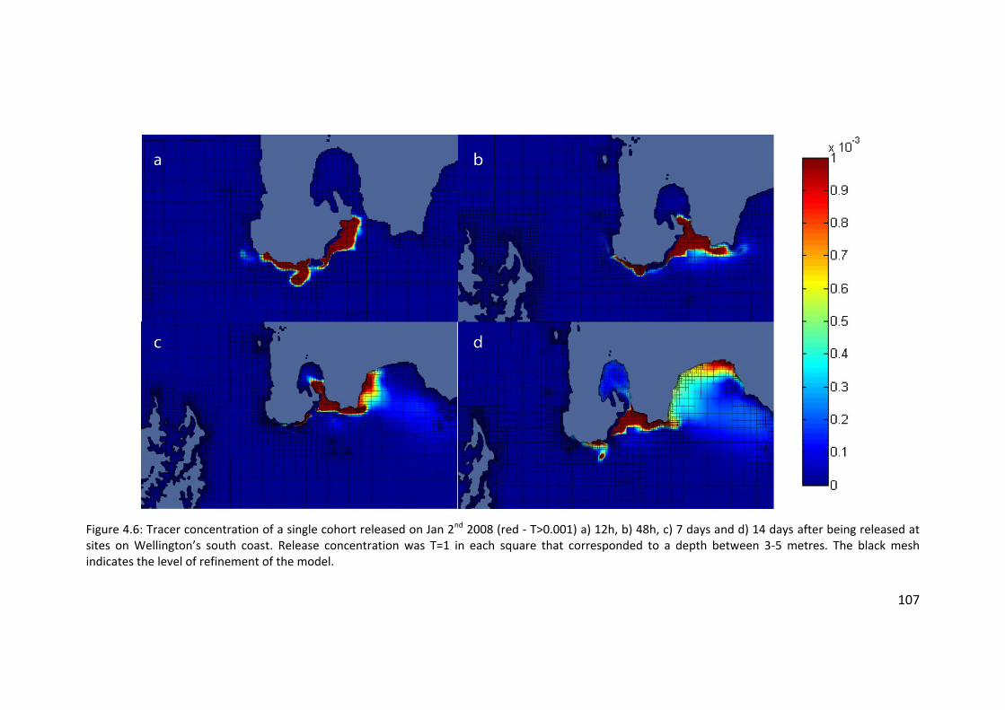
107
Figure 4.6: Tracer concentration of a single cohort released on Jan 2nd 2008 (red - T>0.001) a) 12h, b) 48h, c) 7 days and d) 14 days after being released at sites on Wellington’s south coast. Release concentration was T=1 in each square that corresponded to a depth between 3-5 metres. The black mesh indicates the level of refinement of the model.
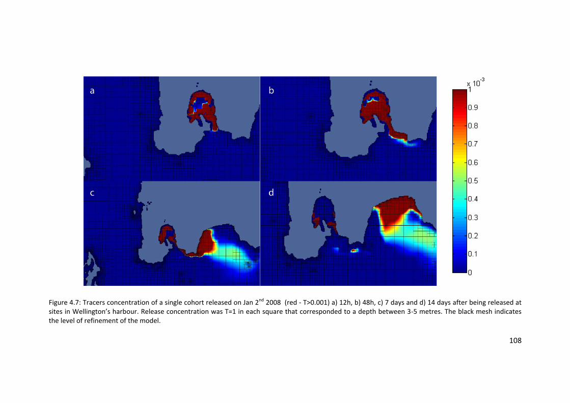
108
Figure 4.7: Tracers concentration of a single cohort released on Jan 2nd 2008 (red - T>0.001) a) 12h, b) 48h, c) 7 days and d) 14 days after being released at sites in Wellington’s harbour. Release concentration was T=1 in each square that corresponded to a depth between 3-5 metres. The black mesh indicates the level of refinement of the model.
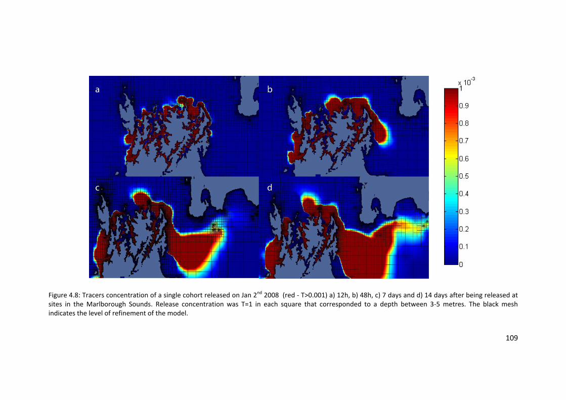
109
Figure 4.8: Tracers concentration of a single cohort released on Jan 2nd 2008 (red - T>0.001) a) 12h, b) 48h, c) 7 days and d) 14 days after being released at sites in the Marlborough Sounds. Release concentration was T=1 in each square that corresponded to a depth between 3-5 metres. The black mesh indicates the level of refinement of the model.

110
Figure 4.9: Mean ccurrent velocities and directions in Cook Strait as predicted by the Gerris flow solver ocean model for the period of the study. Colours and vectors are scaled to a maximum velocity of 1m/s (red) and displayed at a maximum of 8 refinement steps for visualization purposes.
Chapter 4. Larval dispersal pathways in a reef fish metapopulation
111
The patterns described above were sustained over extended periods of
time (and well beyond the week displayed in the figures), however at ever
diminishing proportions due to a single release of tracers. Even after three
weeks a small portion of tracers still leave the Marlborough sounds to
travel towards Wellington. The same holds for Kapiti and Wellington.
Similarly, a proportion of larvae remain retained at all sites for extended
periods of time.
4.3.3 Comparing otolith and simulation results
Many of the connections found by otolith chemistry are supported by
the tracer movements in the hydrodynamic model (Figure 4.10). Both, self-
recruitment and south-eastward dispersal of F. lapillum larvae are found
empirically (Figure 4.3 & 4.10) and are evident from passive tracers (Figure
4.5-4.8). However, dispersal from Wellington to Kapiti Island is inferred by
otolith chemistry but is not predicted by the passive dispersal model
(Figure 4.10). While none of the dispersers at Long Island are assigned to
Kapiti Island by the classification model, there is some, if little, probability
mass associated with this dispersal pathway, which is supported by
hydrodynamic simulations.
4.4 Discussion
Larval dispersal in the ocean is a notoriously complex phenomenon to
describe both empirically and by simulation (Levin 2006, Cowen et al. 2007,
Zimmer et al. 2009). Complex larval behaviours, potentially arising as
evolutionary adaptations to local flow regimes or patchy habitat (Byers &
Pringle 2006, Baskett et al. 2007), make it difficult to appreciate the worth
of simulation studies without any empirical verification. Similarly, results of
dispersal obtained on ecological timescales are generally snapshots of
connectivity in a system, and assuming generality of such snap-shots may
lead to misconceptions about dispersal patterns in a system. The premise

4.4 Discussion
112
Figure 4.10: Dispersal pathways inferred by otolith chemistry (arrows). Blue arrows indicate support from the hydrodynamic simulations for these pathways; the red arrow depicts a pathway for which there is no evidence from the passive dispersal model. Arrow widths are proportional to the mean of the posterior distribution of inferred proportions of larvae dispersed along each pathway. Only connections with a posterior mean of >0.05 are displayed.
of this study was to compare a snap-shot of empirically observed
connectivity with predictions about the dispersal of passive simulated
larvae obtained from a fine scale hydrodynamic model in order to infer the
existence of predicted pathways on an ecological time-scale and to gain
mechanistic insight into the drivers of observed dispersal patterns in the
system.
Empirical results suggest that regions are supplied by a mix of locally
spawned larvae and larvae originating from distant sites. This is consistent
with an emerging view that most local marine populations are sustained by
a mixture of locally produced and distance-sourced recruits, albeit
differences between species in larval durations and behaviours (e.g.
Almany et al. 2007). The degree to which sites are supplied by self-
recruited or dispersed recruits is likely due to local physical conditions
Chapter 4. Larval dispersal pathways in a reef fish metapopulation
113
interacting with larval behaviours. Shanks et al. (2003) suggest that there
are essentially two modes of dispersal: larvae either disperse far and or
hardly disperse at all, attributing the latter to behavioural adaptations (see
also Shanks 2009). The hydrodynamic model provides a null hypothesis of
passive dispersal (Shanks 2009) and results suggest that some of the
patterns observed here may be due to passive mechanisms alone: Larvae
are retained in all regions for extended periods of time throughout the
simulation. This may be somewhat surprising in Kapiti, where strong
alongshore currents develop (Chiswell & Stevens 2010). Since F. lapillum
deposit their eggs in very shallow water however, a loss of current speed
close to shore may help larvae to be retained near spawning sites (Shanks
& Kipp Shearman 2009). The refined grid along the coast in the model
employed here may be particularly useful in capturing this phenomenon,
which may be difficult to reproduce with a fixed grid model.
It may be easier to appreciate that enclosed locations, such as
Wellington Harbour, may passively retain larvae in enclosed bays away
from the harbour mouth and strong tidal currents. Otolith chemistry
provides some support of retention in enclosed bays: In the Marlborough
Sounds recruit otolith chemistry suggests that regional self-recruitment is
due to larvae spawned within the inner Queen Charlotte Sound while
dispersed larvae seem to have come from sites towards the opening of
upstream Pelorus sound. Self-recruitment may therefore be a rather
prevalent mode of replenishment for many of the local populations in the
strait. This is supported by recent research in the Wellington region using
the same study species (Shima & Swearer 2009b, Swearer & Shima 2010)
as well as by a recent genetic study which found significant differentiation
between some populations in a prevalent intertidal snail in and around
Cook Strait (Salinas de Leon et al. – in review). Such self-recruitment in the
sites covered by this study is not necessarily associated with larval homing
behaviour – it may be explained by passive mechanisms in enclosed and
4.4 Discussion
114
shallow bays as well as in retentive eddies forming on complex coastlines
(Mace & Morgan 2006).
While self-seeding is evident for F. lapillum from both the
hydrodynamic model and otolith chemistry, so is dispersal between regions
and their marine reserves. Most connections inferred by otolith chemistry
are readily explained by the prevailing current through Cook Strait: the
D’Urville current flows through the Strait, moving water-masses in a south-
easterly direction before encountering and mixing with the Southland
current (Heath 1985). This is reflected in dispersal of tracers from Kapiti
and the Marlborough Sounds in the hydrodynamic model which predicts
both of these connections. Dispersal from the upper-Marlborough Sounds
(i.e. Pelorus Sound) to Long Island and dispersal from Kapiti Island to
Wellington can be attributed to dispersal of larvae within this mean current
(Figure 4.10). Downstream connections thus seem to be prevalent and
contribute recruits to populations in both Islands.
Dispersal evidenced empirically is restricted to within-Island exchange
of larvae. The hydrodynamic model predicts that passive propagules from
the Marlborough sounds should move towards the lower part of the North
Island, but the sample size in this study may not be large enough to detect
this connection if only a few larvae make or survive such a journey. Shima
& Swearer (2009a, 2010) found that dispersal out of inshore waters (i.e.
Wellington Harbour) may lower a disperser’s fitness and subsequent
survival for F. lapillum. Fish may therefore be adapted to avoid such long
distance dispersal by aiming to stay near high resource waters.
Alternatively, few larvae may actually survive long periods in food depleted
waters and or may have low fitness at arrival and thus do not survive for
long post-settlement.
More intriguingly however, otolith chemistry indicates that dispersal
may also happen against the prevailing current in this system (Figure 4.10).
Chapter 4. Larval dispersal pathways in a reef fish metapopulation
115
While the hydrodynamic model shows that a proportion of tracers released
in Wellington get swept upstream by tidal motion, there is no support from
the model for these empirical results. However, Heath (1986) found a
north-westward mean flow north-west of Wellington. I find that a fraction
of passive tracers disperse in this direction before being captured and
driven south-eastward by the mean flow in Cook Strait. Nevertheless, such
conditions may be accentuated by strong southerly winds (Chiswell &
Stevens 2010) and could be responsible for transport of larvae against the
overall mean current through the Strait. Theory predicts that selective
pressure in advective environments will lead to adaptations to counter
advection and loss of propagules (Byers & Pringle 2006). The use of current
variability has been predicted (Shanks & Eckert 2005) and empirically
shown to help near-shore species avoid advection in mean currents
(Breitburg et al. 1995, Paris & Cowen 2004, Morgan & Fisher 2010) and
may allow populations to be maintained at the upstream edge of species
distributions (Byers & Pringle 2006). Such variability, coupled with larval
behaviour, could thus permit larvae to disperse against overall mean
currents, and may have led to the patterns evidenced by otolith chemistry.
As Kapiti and Wellington have overlapping distributions of geochemical
signatures (Figure 2.3, Chapter 2), an alternative explanation for larvae
dispersing from Wellington to Kapiti could be that these larvae are simply
being miss-assigned to Wellington. This seems unlikely however since it is
the assignments to Kapiti that are predominantly associated with low
classification probabilities. Most fish attributed to Wellington displayed
high classification probabilities. Alternatively, some sources further
upstream with a signature similar to that of Wellington Harbour may have
contributed to recruits at Kapiti. This seems unlikely since model generated
predictions and personal observations do not suggest that other local
populations of substantial abundance and thus potential sources exist
along this coastline.
4.4 Discussion
116
A number of fish were attributed to sites other than the sampled ones
within each region. In Wellington, for instance, fish that seemed to be self-
recruited did not associate with baseline samples. Post-hoc examination of
this cluster revealed higher P and S concentrations. These fish may have
been spawned near the river mouth of Hutt River, which enters Wellington
Harbour. These sites were not sampled for eggs to construct the baseline
due to high turbidity, but Hutt river discharge may explain these values.
This is supported by comparatively high Ba values in the core which may be
produced by a freshwater source (Hamilton & Warner 2009).
This study demonstrates how empirical and simulation results can give
complementary results which provide insight into dispersal mechanisms at
play in a given system (see also Gilg & Hilbish 2003, Nahas et al. 2003,
Ashford et al. 2010): Hydrodynamic model predictions can provide a
physical explanation of dispersal patterns found empirically in the system.
Since retention and passive dispersal with prevailing currents seem to
occur throughout the system, these may be prevalent dispersal modes. The
hydrodynamic model also provides scrutiny for empirical results. I could
not find evidence for dispersal between the two main Islands of New
Zealand, though the model provides some evidence for such a connection:
a more concentrated effort with higher sample sizes could help answer the
question of whether this connection is ecologically relevant. The apparent
upstream connection challenges the assumption of passive dispersal in the
model and indicates that other factors may be at play: I may have missed
an important contributing source for Kapiti Island, or some important
component of dispersal, such as larval behaviour, is not represented by the
model. I investigate these patterns further in chapter 6.
Hydrodynamics can be a strong constraining force, dictating species
distributions (Gaylord & Gaines 2000) and dispersal patterns (Black &
Moran 1991, Gilg & Hilbish 2003, Nahas et al. 2003), but they are rarely

Chapter 4. Larval dispersal pathways in a reef fish metapopulation
117
sufficient to account for measured dispersal patterns (Shanks 2009).
Dispersal of larvae involves a large number of factors, and the complexity
of this phenomenon is unlikely to be described by a single factor and can
thus not be addressed adequately by any single approach. Combining
approaches that bridge time-scales and complement inadequacies
inherent in any single approach is essential to describe connectivity in a
system (Bradbury et al. 2008).

4.4 Discussion
118
119
Chapter 5
5. Plasticity and similarity in dispersal histories: a
Bayesian framework for characterizing fish
dispersal from otolith chemistry profiles
5.1 Introduction
Studying dispersal and migration of larvae and adult animals in the
ocean is essential to understanding population dynamics (Armsworth 2002,
Gaines et al. 2007) and managing exploited and endangered species
(Fogarty & Botsford 2007). Tracking migrations of marine animals is
difficult, especially in species that potentially disperse great distances
and/or remain hidden from direct observation. In fishes, analyses of trace
elements within otoliths (ear-stones) have helped expose life history
characteristics long hidden from direct observation (Campana & Thorrold
2001, Elsdon et al. 2008). Otoliths have, for instance, been used to infer
self-recruitment in reef fish (Swearer et al. 1999), natal homing of
spawning adults to distinct spawning grounds (Thorrold et al. 2001) and
identities of migratory contingents (Secor & Piccoli 1996, Miller et al.
2010). In larval fish, such analyses suggest that different dispersal patterns
may affect larval condition and subsequent juvenile survival (Shima &
Swearer 2009a, 2010).
5.1 Introduction
120
Inferences about fish dispersal made from analyses of otolith chemical
analyses are based on the incorporation of chemical trace elements into
the otolith calcium carbonate matrix: the otolith grows concentrically and
continuously incorporates trace elements from the surrounding
environment. Although not always experimentally verified, elemental
concentrations within the otolith are often assumed to reflect the
surrounding environment (Elsdon et al. 2008). The concentric growth
pattern of otoliths, in conjunction with high resolution sampling techniques
(i.e. Laser Ablation Inductively-Coupled Plasma Mass Spectroscopy (LA-
ICPMS)) makes it possible to study migratory patterns in fish by taking
multiple measurements of elements of interest along the growth axis of an
otolith – this is usually referred to as a transect or profile of otolith
chemistry, which is made up of individual chemical measurements or
‘scans’ (i.e. individual laser ablation pits). Many recent studies use such
profiles along the major otolith growth axis to identify fish movements
amongst chemically distinct water-masses or to differentiate between
groups of fish with similar migratory or dispersal histories (often called
migratory ‘contingents’ (Secor 1999)) (e.g. Secor & Piccoli 1996, Elsdon &
Gillanders 2003, Fablet et al. 2007, Elsdon et al. 2008). Some studies are
based on information about water chemistry and its influence on otolith
chemical composition for a particular species (e.g. Elsdon & Gillanders
2003, Miller et al. 2010). Other studies are based on a set of underlying
hypotheses about environmental influences on otolith chemistry, usually
drawing on a body of literature about such effects (Hamilton et al. 2008,
Shima & Swearer 2009a, Berumen et al. 2010).
A number of different chemical elements and statistical approaches
have been used to infer dispersal histories and associated processes. Fablet
et al. (2007) reviewed a number of studies based on profiles of Sr:Ca as
indicators of freshwater residence. They found that many such studies did
not adequately address the statistical issues inherent in chemical profile

Chapter 5. A Bayesian framework for characterizing fish dispersal
121
data. Many studies rely on visual or ad-hoc characterization of these time
series. Furthermore, measurements (i.e. individual scans or binned means)
along a chemical profile cannot be thought of as independent for a single
fish, and ignoring such non-independence can be problematic.
Elsdon et al (2008) proposed to use repeated measures ANOVA (RM-
ANOVA) or its mixed model extension as a framework to test for
differences in groups of fish over time, and this has by far been the most
prevalent method of analysis for this type of data. While RM-ANOVA
provides some desirable features - one may for instance test the influence
of water chemistry or age on observed differences - it also has substantial
drawbacks. For instance, the ecological meaning of a significant difference
between chemical profiles is not intuitively clear: a result of statistically
significant differences in profiles tells little about the nature of these
differences. Pairwise differences between scans in the profile can be used
(Berumen et al. 2010), but this becomes cumbersome with high resolution
transects and a decent number of samples. Furthermore, one may wish to
analyse time series of variable length to account for age differences in fish.
This makes the application and interpretation of (mixed model) repeated
measures ANOVA difficult. Other approaches have been proposed (Sandin
et al. 2005, Hedger et al. 2008, Shima & Swearer 2009a), but of these
methods only the approach of Hedger et al. provides time-resolved
information about dispersal patterns. Other methods find ways to
characterize contingents but do not provide other relevant descriptions of
dispersal or migration history.
Fablet et al. (2007) realized the need for a statistical framework which
effectively addresses the shortcomings in previous analyses and proposed
a sequential analysis of otolith chemical profiles based on latent state
models. These ‘latent states’ are in fact the hidden environments or water-
masses through which fish disperse. Their study is the first to construct

5.2 Methods
122
generative probabilistic models from hypotheses or knowledge of
processes that lead to measured profiles. For instance, if fish are thought
to move from estuarine to marine environments at different ages or with
different probabilities one may construct a model which reflects the
differences in otolith chemistry that are produced by each environment
and which explicitly models parameters of interest, such as residence times
in each environment or probabilities of movement between environments.
While their paper is an important step towards a statistically rigorous
treatment of such chemical profiles and associated ecological parameters
of interest, Fablet et al. (2007) stop short of a general framework.
Furthermore, although stated as a Bayesian analysis, their sequential
analysis does not 'propagate' uncertainty, and their results are (maximum
likelihood) point estimates rather than Bayesian posterior distributions
(their paper is Bayesian from the use of Bayes theorem to compute the
most likely sequence of states for each fish. The inference presented is,
however, not Bayesian). In this paper I build on the general idea of a
probabilistic framework for modelling otolith profiles. I propose a general,
fully Bayesian approach using latent state models, which I suggest as a
flexible and powerful framework for analysing fish dispersal. To show how
this framework can be used to accommodate and test a number of
relevant ecological hypotheses, I first use a simple mixture model from
which it is possible to infer residence and transition between
environments, as well as test the influence of external parameters (i.e. age)
on inferred dispersal histories. I then propose two measures of similarity of
dispersal histories which provide a new method to characterize migratory
contingents. An accompanying visualization approach allows one to gain
further insight into the nature of dispersal histories of inferred contingents.
I lastly discuss how different approaches to model selection can help find
appropriate models for a given dataset.
Chapter 5. A Bayesian framework for characterizing fish dispersal
123
5.2 Methods
5.2.1 Generative models for chemical transects
It is often possible to make predictions about the influence of certain
water-masses on otolith chemistry, regardless of whether prior knowledge
or hypotheses constructed from known patterns are used. To formally
construct such a generative model for time series of chemical measures
across otoliths, the generative hypothesis needs to be expressed in
probabilistic terms. Coding as y = yi;1; : : : ; yi;t; : : : ; yi;Ty = yi;1; : : : ; yi;t; : : : ; yi;T the TT
measurements made across the otolith of fish ii (other parameters are
indexed accordingly), the time series can be written as a mixture of KK
different environmental (or water-mass) signatures which fish ii
(i = 1; : : : ; N)(i = 1; : : : ; N) experienced. The joint density of y = (y1:::y :::y )y = (y1:::y :::y ) can
then be written as:
f(yj¼; µ) =
NY
i=1
TY
t=1
KX
k=1
¼i;kf(yi;tjµk)f(yj¼; µ) =
NY
i=1
TY
t=1
KX
k=1
¼i;kf(yi;tjµk) (5.1)
where f (yi;tjµk)f (yi;tjµk) is the probability density of the distribution (parameterized
by µkµk) associated with environment kk evaluated at yi;tyi;t. A proportion of
the signatures along the profile of individual ii are generated by
environment kk, reflecting residency in this environment for this proportion
of time. ¼ = (¼i; 1:::¼i; k:::¼i; K)¼ = (¼i; 1:::¼i; k:::¼i; K) and ¼ = (¼1:::¼i:::¼N )¼ = (¼1:::¼i:::¼N ) then denote the
vector over all source proportions for individual ii, and the set of vectors of
source proportions for all individuals, respectively. It is commonly assumed
that different chemical measures pertaining to a given environment
experienced by a fish follow a (multivariate) normal distribution, such that
µk = f¹k;§kgµk = f¹k;§kg, with µ = (µ1:::µk:::µK)µ = (µ1:::µk:::µK) for the KK sources, although other
continuous distributions may be used. This model assumes independence
in measurements along the otolith profile, a property which I discuss
further on.

124
Figure 5.1: Upper panels: Example profiles for Strontium and Barium across Chinook salmon otoliths. Lower panels: Histograms of count frequency for Strontium and Barium measures for all N Chinook salmon from Miller et al (2010).
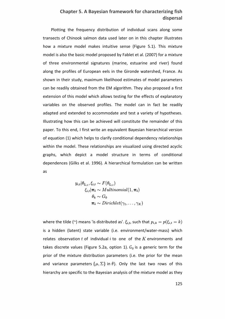
Chapter 5. A Bayesian framework for characterizing fish dispersal
125
Plotting the frequency distribution of individual scans along some
transects of Chinook salmon data used later on in this chapter illustrates
how a mixture model makes intuitive sense (Figure 5.1). This mixture
model is also the basic model proposed by Fablet et al. (2007) for a mixture
of three environmental signatures (marine, estuarine and river) found
along the profiles of European eels in the Gironde watershed, France. As
shown in their study, maximum likelihood estimates of model parameters
can be readily obtained from the EM algorithm. They also proposed a first
extension of this model which allows testing for the effects of explanatory
variables on the observed profiles. The model can in fact be readily
adapted and extended to accommodate and test a variety of hypotheses.
Illustrating how this can be achieved will constitute the remainder of this
paper. To this end, I first write an equivalent Bayesian hierarchical version
of equation (1) which helps to clarify conditional dependency relationships
within the model. These relationships are visualized using directed acyclic
graphs, which depict a model structure in terms of conditional
dependences (Gilks et al. 1996). A hierarchical formulation can be written
as
yi;tjµ»i;t; »i;t » F (µ»i;t
)
»i;tj¼ »Multinomial(1;¼ )
µk » G0
¼ » Dirichlet(°1; : : : ; °K)
yi;tjµ»i;t; »i;t » F (µ»i;t
)
»i;tj¼ »Multinomial(1;¼ )
µk » G0
¼ » Dirichlet(°1; : : : ; °K)
where the tilde (~) means 'is distributed as'. »i;t»i;t, such that pi;k = p(»i;t = k)pi;k = p(»i;t = k)
is a hidden (latent) state variable (i.e. environment/water-mass) which
relates observation tt of individual ii to one of the KK environments and
takes discrete values (Figure 5.2a, option 1). is a generic term for the
prior of the mixture distribution parameters (i.e. the prior for the mean
and variance parameters f¹;§gf¹;§g in µµ ). Only the last two rows of this
hierarchy are specific to the Bayesian analysis of the mixture model as they

5.2 Methods
126
specify prior distributions on hyper-parameters. Note also that the
multinomial distribution collapses to a binomial one if only two
environments are of interest. The generative model can be expressed as
follows: Fish ii experiences one of KK water-masses at time tt. This water-
mass is drawn from a distribution of possible environments with
probability ¼i;k¼i;k . The observed signature is then generated from the
distribution (i.e. N (µk)N (µk)) associated with this environment.
This model can be readily extended to test for the effects of covariates
xx (i.e. age, temperature) on observed transects by adding a line to the
hierarchical formulation, such that
¹jx; a; b;§ » N(a+ bx;§¹)¹jx; a; b;§ » N(a+ bx;§¹).
This setup specifies a simple regression relationship (Figure 5.2a,
option 2) for the parameter ¹¹. Often it is the sequence of environments
visited or the use of environments that is of primary interest (Fablet et al.
2007, Shima & Swearer 2009a, 2010). These parameters are estimated as
»» and ¼¼ of the model. Covariates can be included in a similar way to model
some effect on the parameter ¼¼. An older fish, for instance, may be more
likely to have visited a spawning ground than a juvenile. One could thus
relate ¼¼ to the age of the fish by using a prior for individual °°, the prior
‘counts’ for ¼¼ .
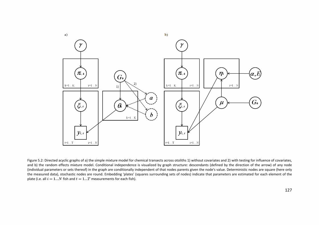
127
Figure 5.2: Directed acyclic graphs of a) the simple mixture model for chemical transects across otoliths 1) without covariates and 2) with testing for influence of covariates, and b) the random effects mixture model. Conditional independence is visualized by graph structure: descendants (defined by the direction of the arrow) of any node (individual parameters or sets thereof) in the graph are conditionally independent of that nodes parents given the node's value. Deterministic nodes are square (here only the measured data), stochastic nodes are round. Embedding ‘plates’ (squares surrounding sets of nodes) indicate that parameters are estimated for each element of the plate (i.e. all i = 1:::Ni = 1:::N fish and t = 1:::Tt = 1:::T measurements for each fish).
128
5.2.2 The Bayesian approach: Prior knowledge and the lack thereof
The remainder of this chapter is based on the Bayesian treatment of the
general model outlined in equation (5.1). There are multiple reasons for this. I
already mentioned that the Bayesian approach can accurately reflect uncertainty
about all parameters in the model. Another advantage is that the quantities I will
use below to define similarity of profiles are readily available from a Bayesian
treatment of the model.
Encoding prior information can be helpful in analysing chemical profiles, and
this information is a fundamental quantity in Bayesian analysis. Studies which
experimentally relate environmental factors to otolith chemistry can for instance
be used to construct prior distributions for environments, which in turn can
facilitate estimation of dispersal histories and other parameters. I illustrate this
with the Chinook salmon example later on. Similarly, information about the effects
of age or growth on the incorporation of chemicals into the otolith may be
available. This information could be encoded as priors on the above regression
formula.
Bayesian approaches are sometimes criticized for the fact that the prior
probability is part of the analysis, even when no substantial information exists.
Often, it is possible to find formulations for prior distributions which convey
minimal information (so-called vague priors). Such vaguely informative priors
however can lead to problems with estimation of latent state models: the labels
that are given to the environments become meaningless in the model and »» will
change 'identity' throughout the estimation of this model - the so-called 'label
switching' problem. A simple but effective way to re-parameterize the model is by
expressing the means of different environments in an additive fashion, such that
¹2 = ¹1 + ¿¹2 = ¹1 + ¿ and restricting tau to be positive. Such problems can also be dealt with
by using informative priors for the parameters of different mixture components
(i.e. one might suspect that values of some chemicals are higher in rivers than the
Chapter 5. A Bayesian framework for characterizing fish dispersal
129
ocean or vice versa), which therefore make the model formulation and estimation
somewhat easier.
5.2.3 Encoding alternate hypotheses
Testing for covariate effects is but one application of the above model. I now
illustrate how this model can be used to encode alternate hypotheses - or the lack
of strong hypotheses. For example, there may be considerable variability in the
signatures of an environment, for estuarine species for instance, substantial
variation in salinity within an estuary may lead to variability in Sr signatures
depending on which part of the estuary a fish resided in. Assuming that the
environmental signatures are normally distributed, a natural extension is then a
hierarchical model for individual environmental means (a random effects model).
In the next chapter I use this model for reef fish recruits to estimate nearshore
residency of these fish during their larval period. In that case there are thought to
be multiple larval origins along a coast that exhibit variability in the distribution of
signatures among nearshore spawning habitats. Thus, one may not have just one
distribution for larvae spawned and residing nearshore, but rather a number of
them which are linked via common prior. This model can be encoded by modifying
the first line of the above model to read
yi;tjµ»i;t; »i;t » N(¹+ »i;t´i;§»i;t)
´ij®; & » N(®; &)
yi;tjµ»i;t; »i;t » N(¹+ »i;t´i;§»i;t)
´ij®; & » N(®; &)
µµ now includes only the mean and variance of the water-mass(es) without a
random effect. All other lines are identical to the original model (Figure 2b). Note
that the means have an additive parameterization. ´i´i can now be restricted to be
positive (or give an informative prior) to ensure identifiability of the mixture. »i;t»i;t is
1 if a nearshore environment is drawn and zero otherwise, and the random effect is
thus only used for nearshore means ´i´i. The nearshore characteristic (or random
effects) distribution, from which individual nearshore means are drawn, is thus
found at a lower level of the hierarchy. The above formulation suggests that
variances of water-masses may be different, but one may choose to model
5.2 Methods
130
variances of different water-masses as constant (this raises the question of how
one actually defines a water-mass or environment, which I will discuss below).
This model may also be useful if fish migrate from the ocean to different
tributaries in an estuary or a river system or vice versa. Variations on this setup
would include random effects on means of each environment: fish may move from
different rivers to different estuaries and end up in a mixed stock in the ocean.
Flexibility can be added for both environments, provided that it is possible to
distinguish between rivers and estuaries globally. The ease with which such
hierarchical models can be implemented in a Bayesian setting is an additional
argument in favour for adopting a Bayesian approach (Clark 2003).
A further hypothesis would be that most fish display variations of the same
migratory behaviour, and are thus expected to spend related amounts of time in a
given environment. Two options come to mind: one may use a common mixture
distribution ¼¼ for all transects, or alternatively place a hierarchical prior on ¼¼. The
former assumes that all fish share the same behaviour parameterized by ¼¼, while
the latter assumes that each fish performs a variation of an inert behaviour. Both
may be valid assumptions, and both allow information about behaviours to be
shared between individual time-series. However, the hierarchical option is
considerably more flexible. Rather than specifying the prior °1; : : : ;°K°1; : : : ;°K for ¼i;K¼i;K
independently for each fish (°1; : : : ; °K = 1°1; : : : ; °K = 1 is, for instance, often used as a ‘vague’
prior, see below), one may specify a common prior for the mixing proportions, i.e.
°k » Gamma(u; v)°k » Gamma(u; v).
5.2.4 Estimating the number of (distinguishable) environments along a
transect
A further motivation for a Bayesian analysis of dispersal comes from the
possibility to actually estimate the number of distinct environments a fish may
have experienced (see also chapter 3). In a dispersal study it may be of interest to
know how many distinct (or distinguishable) water masses are reflected on the
profiles of the sampled fish. The Bayesian approach allows us to place a prior on
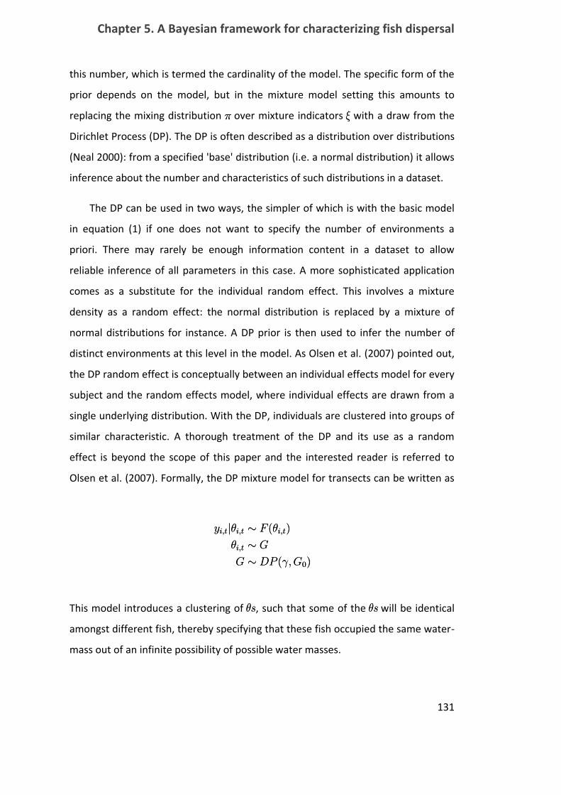
Chapter 5. A Bayesian framework for characterizing fish dispersal
131
this number, which is termed the cardinality of the model. The specific form of the
prior depends on the model, but in the mixture model setting this amounts to
replacing the mixing distribution ¼¼ over mixture indicators »» with a draw from the
Dirichlet Process (DP). The DP is often described as a distribution over distributions
(Neal 2000): from a specified 'base' distribution (i.e. a normal distribution) it allows
inference about the number and characteristics of such distributions in a dataset.
The DP can be used in two ways, the simpler of which is with the basic model
in equation (1) if one does not want to specify the number of environments a
priori. There may rarely be enough information content in a dataset to allow
reliable inference of all parameters in this case. A more sophisticated application
comes as a substitute for the individual random effect. This involves a mixture
density as a random effect: the normal distribution is replaced by a mixture of
normal distributions for instance. A DP prior is then used to infer the number of
distinct environments at this level in the model. As Olsen et al. (2007) pointed out,
the DP random effect is conceptually between an individual effects model for every
subject and the random effects model, where individual effects are drawn from a
single underlying distribution. With the DP, individuals are clustered into groups of
similar characteristic. A thorough treatment of the DP and its use as a random
effect is beyond the scope of this paper and the interested reader is referred to
Olsen et al. (2007). Formally, the DP mixture model for transects can be written as
Formally the DP mixture model for transects can be written as
yi;tjµi;t » F (µi;t)
µi;t » G
G » DP (°; G0)
yi;tjµi;t » F (µi;t)
µi;t » G
G » DP (°; G0)
This model introduces a clustering of µsµs, such that some of the µsµs will be identical
amongst different fish, thereby specifying that these fish occupied the same water-
mass out of an infinite possibility of possible water masses.
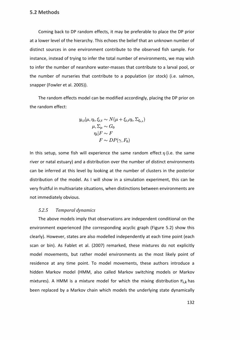
5.2 Methods
132
Coming back to DP random effects, it may be preferable to place the DP prior
at a lower level of the hierarchy. This echoes the belief that an unknown number of
distinct sources in one environment contribute to the observed fish sample. For
instance, instead of trying to infer the total number of environments, we may wish
to infer the number of nearshore water-masses that contribute to a larval pool, or
the number of nurseries that contribute to a population (or stock) (i.e. salmon,
snapper (Fowler et al. 2005)).
The random effects model can be modified accordingly, placing the DP prior on
the random effect:
yi;tj¹; ´i; »i;t » N(¹+ »i;t´i;§»i;t)
¹;§¹ » G0
´ijF » F
F » DP (°; F0)
yi;tj¹; ´i; »i;t » N(¹+ »i;t´i;§»i;t)
¹;§¹ » G0
´ijF » F
F » DP (°; F0)
In this setup, some fish will experience the same random effect ´́ (i.e. the same
river or natal estuary) and a distribution over the number of distinct environments
can be inferred at this level by looking at the number of clusters in the posterior
distribution of the model. As I will show in a simulation experiment, this can be
very fruitful in multivariate situations, when distinctions between environments are
not immediately obvious.
5.2.5 Temporal dynamics
The above models imply that observations are independent conditional on the
environment experienced (the corresponding acyclic graph (Figure 5.2) show this
clearly). However, states are also modelled independently at each time point (each
scan or bin). As Fablet et al. (2007) remarked, these mixtures do not explicitly
model movements, but rather model environments as the most likely point of
residence at any time point. To model movements, these authors introduce a
hidden Markov model (HMM, also called Markov switching models or Markov
mixtures). A HMM is a mixture model for which the mixing distribution ¼i;k¼i;k has
been replaced by a Markov chain which models the underlying state dynamically
Chapter 5. A Bayesian framework for characterizing fish dispersal
133
(Scott 2002). In a Markov chain the probability of being in state »» at time tt depends
on the state at time t ¡ 1t ¡ 1, and transition between states is governed by a transition
matrix (Figure 5.3). This can be written as written as p(»i;t = kj»i;t¡1 = j) = ¼ikjjp(»i;t = kj»i;t¡1 = j) = ¼ikjj,
where is now a matrix of one-step transition probabilities.
Modelling the state dynamics explicitly can have an important consequence, in
that isolated spikes in readings along a profile are not necessarily attributed to
movements between environments (Fablet et al. 2007). This phenomenon is
usually termed 'filtering' in statistical and engineering jargon. To illustrate the
difference between the mixture model and the HMM, consider a simple example of
a group of fish, each moving once between two chemically distinct environments.
The parameter ¼¼ in the simple mixture model has a natural interpretation of
proportion of time spent in each environment. Assume each fish spends equal
proportions of time in each environment. A point estimate (i.e. the mean of the
posterior distribution) of ¼¼ in the mixture model would then (hopefully) be
around 0.5. Assuming that otolith growth rate is constant or that it is possible to
obtain growth patterns from otolith structural analyses, the proportion ¼¼ is easily
transformed to a measure of how much time fish spend in a particular environment
by multiplying ¼¼ times the total time covered by the profile (i.e. the PLD or age of
the fish).
The transition matrix, however, encodes the probability of movement between
environments, and the above interpretations cannot be readily recovered from the
transition matrix itself. An estimate of a transition matrix in the above example
above would give a low probability to transitions since only one transition occurs
for each fish. For 51 scans of otolith chemistry along a profile for a single fish the
estimated value would thus be around 0.02 for a transition versus 0.98 for resident
behaviour (since there are 50 possible transitions for 51 scans). An estimate of
transition probabilities for only eleven scans would be around 0.1 for a transition
and 0.9 for resident behaviour. The estimates of the transition matrix are thus not
invariant to the sampling frequency and the number of scans.
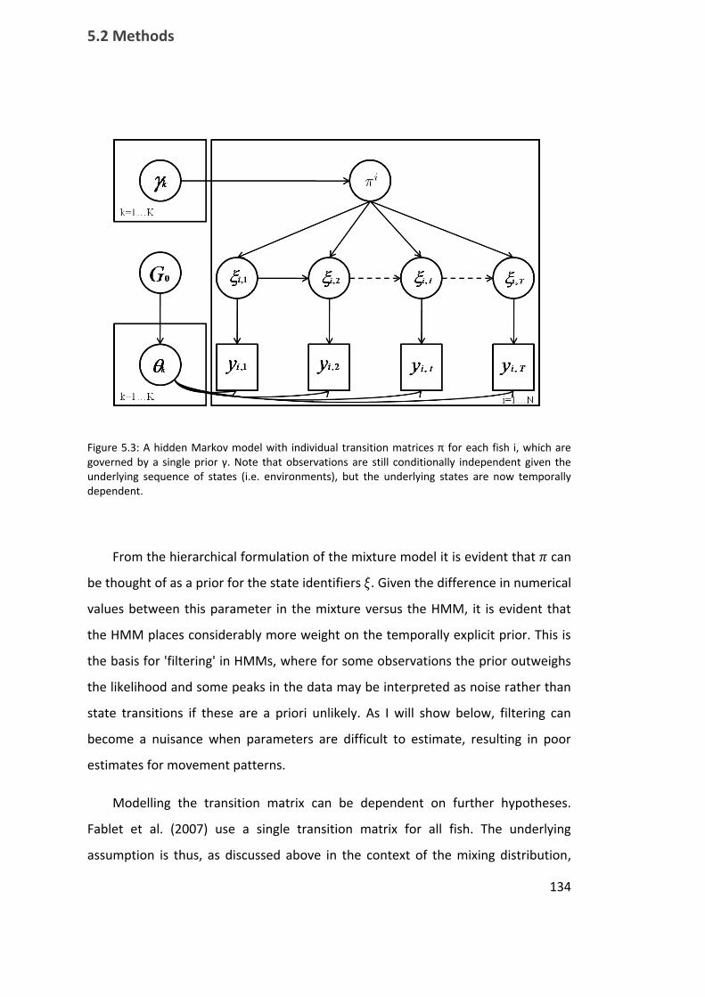
5.2 Methods
134
Figure 5.3: A hidden Markov model with individual transition matrices π for each fish i, which are governed by a single prior γ. Note that observations are still conditionally independent given the underlying sequence of states (i.e. environments), but the underlying states are now temporally dependent.
From the hierarchical formulation of the mixture model it is evident that can
be thought of as a prior for the state identifiers »». Given the difference in numerical
values between this parameter in the mixture versus the HMM, it is evident that
the HMM places considerably more weight on the temporally explicit prior. This is
the basis for 'filtering' in HMMs, where for some observations the prior outweighs
the likelihood and some peaks in the data may be interpreted as noise rather than
state transitions if these are a priori unlikely. As I will show below, filtering can
become a nuisance when parameters are difficult to estimate, resulting in poor
estimates for movement patterns.
Modelling the transition matrix can be dependent on further hypotheses.
Fablet et al. (2007) use a single transition matrix for all fish. The underlying
assumption is thus, as discussed above in the context of the mixing distribution,

Chapter 5. A Bayesian framework for characterizing fish dispersal
135
that all fish have the same a priori propensity to move between a set of
environments. One may instead wish to estimate transitions independently for
each fish, or to give the prior for the transition matrix a hierarchical structure. The
former may be difficult if there are few observations of transitions in each time-
series, whereas the hierarchical approach allows for information about transitions
to be shared across profiles: a common ‘inert’ behaviour is thus assumed. Since the
Dirichlet distribution is commonly used as a prior for each line of the transition
matrix (Cappé et al. 2005), the same prior as for the hierarchical formulation of
mixing distributions may be used. Another alternative is to model a single (common
for all fish), time dependent transition matrix which captures changing propensities
of the sampled fish to move between environments. The Markov Chain is then said
to be non-homogenous. Care must be taken in this case that all fish are aligned
such that individual scans correspond to the same age.
Apart from the Dirichlet process mixture, all of the mixture models developed
in previous sections can be readily transformed into an HMM (though the Dirichlet
random effects models can be used with an HMM). HMMs are, however,
somewhat harder to sample from: the time dependence in the state sequence
renders standard methods of sampling often ineffective. This is discussed in more
detail along with Markov Chain Monte Carlo methods in Appendix 3.
5.2.6 Estimating unknowns: MCMC and WinBUGS
Bayesian approaches can have a drawback in that estimation of unknowns in
the model is difficult and necessitates approximate inference algorithms such as
Markov Chain Monte Carlo and related techniques. I present Gibbs sampling
algorithms for the models I use in the next section in Appendices A2 & A3, where I
also discuss some issues encountered specifically with time explicit models
discussed below. Note that for some of the simple models discussed here,
inference can be straightforward with the freely available Bayesian model building
software WinBUGS (Lunn et al. 2000). I provide some sample code for Winbugs
implementation for simple mixture models in the appendix A4. Dirichlet Processes
5.2 Methods
136
models (see below) can only be approximated by this software and the interested
reader is referred to Ohlsen et al. (2007) for details and sample code. Time
dependencies in Hidden Markov models can make the generic methods in
WinBUGS very ineffective for estimating model parameters, and I therefore only
give efficient Gibbs sampling algorithms in appendix A3. All of the models discussed
in this chapter can be used in a multivariate setting, typically by simply replacing
the distributions for environments and their priors by their multivariate
counterpart.
5.2.7 Characterizing contingents: a marginal visualization approach
A contingent in the context of dispersal refers to groups of fish with distinct
dispersal histories (Secor 1999). A contingent is thus made up of fish with similar
dispersal (migration) history or similar habitat use. This leaves the question of how
one defines this similarity within these groups. An intuitive way to do this is to
define similarity in terms of time that fish spent together (at the same time) in the
same environment. Speaking in terms of the Bayesian models discussed here, this
quantity can be expressed as the marginal posterior probability that a set S of
individuals are found in the same environment at a uniformly chosen time ¿¿ , or
p(»S0;¿ = »S;¿ jy) =Rp(»S0;¿ = »S;¿ jµ)p(µjy)dµp(»S0;¿ = »S;¿ jy) =
Rp(»S0;¿ = »S;¿ jµ)p(µjy)dµ
where S and S' are disjoint sets of fish. This can be estimated from q = (1:::Q)q = (1:::Q)
MCMC samples of the posterior distribution for model parameters µµ as
p(»S0;t = »S;tjy) =1
QT
QX
q=1
TX
t=1
p(»S0;t = »S;tjy; µq)p(»S0;t = »S;tjy) =1
QT
QX
q=1
TX
t=1
p(»S0;t = »S;tjy; µq)
and may be seen as a time averaged form of a co-assignment probability (see
Dawson & Belkhir 2001 for a derivation of this probability). It further marginalizes
over (integrates out) unknowns in the model and thus reflects uncertainty in
parameter estimates.
This definition of (probabilistic) similarity of the time series has a number of
advantages. In fact, this quantity is readily obtained from any MCMC
Chapter 5. A Bayesian framework for characterizing fish dispersal
137
implementation of the above described models: one must simply keep track of the
assignment vector »» at each iteration of the sampler. Furthermore, this definition
of similarity does not involve the actual labels of environments (or states) and is
therefore invariant to label switching. This is a desirable property since it assures
that even without restrictive priors on environment signatures one can still define
similarity. Lastly, this probability can be used in an agglomerative algorithm such as
the exact linkage algorithm (Dawson & Belkhir 2009). This algorithm produces a
tree based on co-assignment probabilities such as defined above, where the node
height is equal to the posterior co-assignment probabilities of the merged sets.
Contingents can be readily inferred on such a tree by assign them a marginal
probability of belonging to the same group.
I introduce a second marginal posterior distribution over the number of
individuals ni;tni;t which at time tt are associated with the same environment as fish ii.
Again, this quantity is easily computed from the MCMC sequence used to estimate
the model and it too is invariant to label switching. Given that this probability is
time indexed, it provides information about temporal structure of the data.
Intuitively, this number will coincide for fish that are associated with the same
environment at time t, and if there is synchronous movement then these numbers
will be constant for the members of a contingent. If trajectories diverge, it can be
easily seen where contingents split or merged on their dispersal pathways. The two
marginal distributions are visualized in a joint plot which associates the tree of co-
assignment probabilities with a matrix image of the ni;Tni;T matrix. Such a
representation is particularly useful for multivariate applications in which visual
differentiation of groups is not straightforward.
5.3 Illustration and validation
I illustrate the merit of the above mentioned models with a series of simulation
experiments. The first experiment includes four distinct scenarios of increasing
complexity to test the performance of different mixture model setups as well as a
5.3 Illustration and validation
138
flexible HMM setup for comparison. A second simulation experiment illustrates
how this method can be used to visualize migratory contingents from multivariate
data, even without specific knowledge of the number of distinct environments
which fish may have resided in. I lastly demonstrate how this modelling framework
can be used on real data to identify plasticity of age at freshwater emigration of
Chinook salmon.
5.3.1 Simulation Experiment I: Increasingly complex simulation scenarios
The first scenario simulated a case of two environments or water-masses, with
each environment characterized by a single normal distribution. Each of 100
simulated fish, for which I simulated transects of 50 individual scans, spent variable
amounts of time in each water-mass. Such a scenario could reflect diadromous fish
which spend variable amounts of time in chemically well characterized habitats (i.e.
Miller et al. 2010). The second scenario was designed as a more complex dispersal
scenario in which fish again spend variable amounts of time in one of two
environments, however one environment is characterized by a number (K=3) of
distinct chemical patterns in collected recruits (i.e. different tributaries or spawning
locations). For the simulation there are three distributions of elevated chemistry
and a single environment with lower chemistry (Table 5.1).
The third scenario is similar to the second in that every simulated fish originates
in one of k=3 locations of elevated chemical concentration, however I introduce an
autocorrelation coefficient of 0.5 to simulate the fact that changes in otolith
chemistry may not be instantaneous.
The last scenario is a relatively complex extension of the second in that each
fish may visit any water-mass on a 3x3 grid (Figure 5.4) with a probability
determined by a transition matrix. Residence in a water-mass is chosen with ’base’
probability pk;k =mpk;k =m. The probability of moving to an adjacent water-mass j on the
grid is pk;j = (1¡ pk;k)=cpk;j = (1¡ pk;k)=c , where cc is the number of adjacent cells. To simulate
aggregative behaviour these probabilities are then transformed to take into
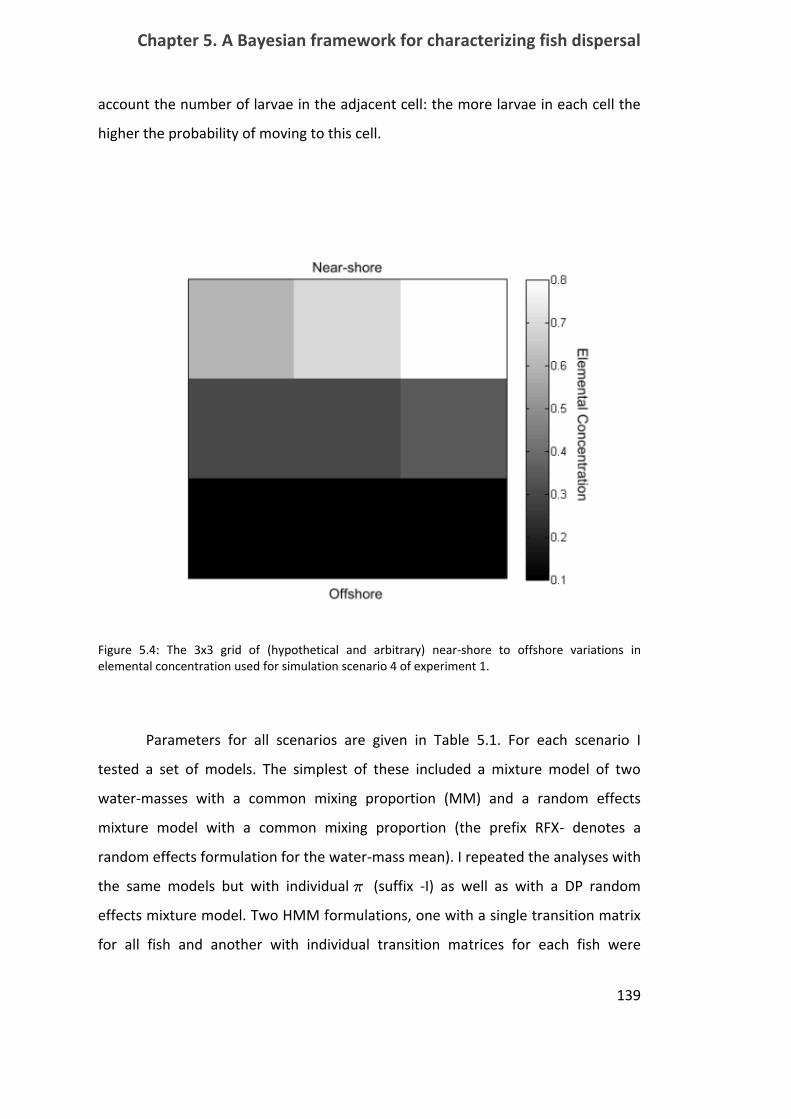
Chapter 5. A Bayesian framework for characterizing fish dispersal
139
account the number of larvae in the adjacent cell: the more larvae in each cell the
higher the probability of moving to this cell.
Figure 5.4: The 3x3 grid of (hypothetical and arbitrary) near-shore to offshore variations in elemental concentration used for simulation scenario 4 of experiment 1.
Parameters for all scenarios are given in Table 5.1. For each scenario I
tested a set of models. The simplest of these included a mixture model of two
water-masses with a common mixing proportion (MM) and a random effects
mixture model with a common mixing proportion (the prefix RFX- denotes a
random effects formulation for the water-mass mean). I repeated the analyses with
the same models but with individual ¼¼ (suffix -I) as well as with a DP random
effects mixture model. Two HMM formulations, one with a single transition matrix
for all fish and another with individual transition matrices for each fish were
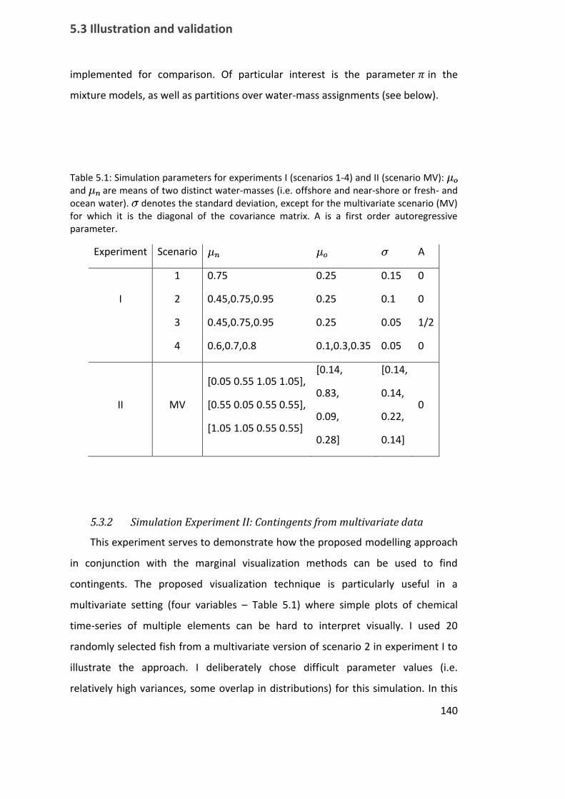
5.3 Illustration and validation
140
implemented for comparison. Of particular interest is the parameter in the
mixture models, as well as partitions over water-mass assignments (see below).
Table 5.1: Simulation parameters for experiments I (scenarios 1-4) and II (scenario MV): ¹o¹o and ¹n¹n are means of two distinct water-masses (i.e. offshore and near‐shore or fresh- and ocean water). ¾¾ denotes the standard deviation, except for the multivariate scenario (MV) for which it is the diagonal of the covariance matrix. A is a first order autoregressive parameter.
Experiment Scenario ¹n¹n ¹o¹o ¾¾ A
1 0.75 0.25 0.15 0
I 2 0.45,0.75,0.95 0.25 0.1 0
3 0.45,0.75,0.95 0.25 0.05 1/2
4 0.6,0.7,0.8 0.1,0.3,0.35 0.05 0
II MV
[0.05 0.55 1.05 1.05],
[0.55 0.05 0.55 0.55],
[1.05 1.05 0.55 0.55]
[0.14,
0.83,
0.09,
0.28]
[0.14,
0.14,
0.22,
0.14]
0
5.3.2 Simulation Experiment II: Contingents from multivariate data
This experiment serves to demonstrate how the proposed modelling approach
in conjunction with the marginal visualization methods can be used to find
contingents. The proposed visualization technique is particularly useful in a
multivariate setting (four variables – Table 5.1) where simple plots of chemical
time-series of multiple elements can be hard to interpret visually. I used 20
randomly selected fish from a multivariate version of scenario 2 in experiment I to
illustrate the approach. I deliberately chose difficult parameter values (i.e.
relatively high variances, some overlap in distributions) for this simulation. In this

Chapter 5. A Bayesian framework for characterizing fish dispersal
141
setup it would be difficult to estimate the true movement patterns from one
element alone. I used the non‐parametric DP-RFX-MM model to resolve similarities
in dispersal histories and examine how well the non‐parametric method performs
at estimating common dispersal patterns and the number of water-masses present
in the profiles. Both may not be immediately obvious from multivariate time series.
5.3.3 Assessing models: posterior predictive checks and model selection
I applied the above mentioned models to the simulation scenarios to find the
limits and strengths of the respective models. To compare models in terms of their
adequacy for the data at hand I employed a number of model selection tools.
The natural approach for this in a Bayesian analysis is the Bayes factor, which is
the ratio of integrated (also called marginal) likelihoods, in other words the ratio of
model likelihoods integrated over unknown parameters (Kass & Raftery 1995). The
Bayes factor can be thought of as a Bayesian analogue of the likelihood ratio test,
where rather than maximizing the likelihood with respect to unknown parameters,
these are integrated over in the posterior distribution. The advantage of the Bayes
factor is that it automatically penalizes complex models if these are not justified. A
ratio of 10:1 is generally seen as strong evidence in favour of the better model, a
ratio of >100:1 shows decisive evidence in favour for the winning hypothesis (Kass
& Raftery 1995). The Bayes factor is somewhat difficult to compute, especially in
more complex models such as DP models, and I reserved this for models of real
data. Specifically, I used the method of Chib (1995) to estimate the marginal
likelihood in the next section (5.3.4). The use of informative priors in that section
assures that sensitivities of Bayes factors to non-informative priors are of minor
concern in this case.
For the simulation studies, I examined estimated quantities and looked at data
generated from the posterior predictive distribution to check for consistency of
these mixture models with the real data ‐ if simulated data from this distribution is
far from the real data in terms of predefined characteristics (i.e. the spread in the
data), the model is deemed inadequate (Gelman et al. 2003). While this does not

5.3 Illustration and validation
142
give a measurable quantity for model comparison in a Bayesian sense, it will
indicate model adequacy and can thereby serve to point out (in-) appropriate
models.
To evaluate model fit I checked whether the proposed models were able to
reflect the spread in the data by calculating the posterior predictive test quantity
E(¢Y ) = 1Q
PQ
q=1(max(y )¡min(y ))¡ (max(y )¡min(y ))E(¢Y ) = 1Q
PQ
q=1(max(y )¡min(y ))¡ (max(y )¡min(y )),
where yy is data simulated from the posterior predictive distribution
p(y jy) =Rp(y jµ)p(µjy)dµp(y jy) =
Rp(y jµ)p(µjy)dµ for concentrations yy and the expectation EE is
calculated over QQ MCMC samples from the posterior distribution. For mixture
models I also calculated E(¢¼) = 1NQ
PQ
q=1
PN
i=1(¼i;q ¡ ¼Mi;q)E(¢¼) = 1NQ
PQ
q=1
PN
i=1(¼i;q ¡ ¼Mi;q) for all simulations,
where ¼M¼M is the estimated posterior distribution of the paramter ¼¼ in the model.
The latter quantity simply verifies whether the model accurately estimates the true
mixing proportions.
To illustrate the advantages and drawbacks of these models, I compared the
modal partitions of each model to the original partition (i.e. the mode of the
posterior distribution of »»). A partition is simply the set of assignments of scans to
water-masses (the »s»s in the model). In the case of two water-masses, this would be
a set of 0s and 1s for each fish. With DP random effects models, one could also
choose to use the partition that includes assignment to a given random effects
water-mass. One would then use a set of arbitrary numbers for each water-mass.
The same applies to setups with more than two water-masses. The mean partition
is then simply the partition that minimizes the sum of squared distances from the
partitions observed during the MCMC. These partitions however are not invariant
to label switching and I use them for illustrative purposes only – all models used for
simulations use identifiability constraints on the means of water-masses.

Chapter 5. A Bayesian framework for characterizing fish dispersal
143
5.3.4 Application to Chinook salmon
To test the performance of these models in the real world, I applied a hidden
Markov model to a set of Barium (Ba) and Strontium (Sr) profiles across otoliths of
adult Chinook salmon. These data have previously been analysed by Miller et al.
(2010) to estimate fork length at freshwater emigration (FL) of fish originating in
the Central California Valley. Their study found that fish emigrate at a variety of FLs,
and that medium sized individuals (‘parr’) represent the majority of emigrating
juveniles.
FL at emigration was calculated from otolith width (OW) at emigration, with
OW itself taken at a threshold point where substantial changes in otolith chemistry
occur. Specifically, at freshwater emigration, Sr tends to increase, reflecting higher
availability with increasing salinities. Similarly, Barium tends to decrease
substantially as salinity increases. A series of experiments and empirical
observations lead to predictions about otolith chemistry in the different
environments of interest. These predictions in turn allowed the authors to define a
threshold for ocean and freshwater signatures. A third category, brackish water,
seemed to be present in the measured chemistry, with higher Barium than ocean
waters and Strontium values approaching those of ocean water.
The proposed thresholds depended on a number of models and observations
relating otolith chemistry to water chemistry. As noted by Miller et al. (2010), the
observed chemistry of some of the adult fish collected falls outside of the predicted
confidence intervals. For ocean residence for instance, only 44 % of fish fell within
the predicted Sr range, while only 12% fell within the predicted Ba range. There is
thus clearly a limit to the underlying models and hence the proposed thresholds. I
show how HMMs can be used to estimate habitat transitions from both the
previous predictions and the current data at hand. I show how the methods
presented in this chapter can be used to obtain (marginal) posterior over
parameters of interest in the original study, as well as additional quantities
estimated from the models.
5.3 Illustration and validation
144
I used a hidden Markov model to reconstruct movements since these tend to
filter more noise and will allow for a more accurate estimation of the OW at
emigration. Random effects were used for the freshwater signatures, reflecting the
contribution of different tributaries and/or varying strength in
maternal/physiological effects on observed freshwater signatures. I added a third
category of brackish water and tested this model against a model with only two
water-masses using the Bayes factor. I could have fixed the HMM transition matrix
since we know that across the profile, which spans the entire otolith, one transition
from ocean- to freshwater and one transition from fresh- to ocean water will be
observed. Given the relatively clear pattern however, results are virtually identical
and I report results with estimated transition matrices.
While it is possible to include the regression models that lead to predictions
about otolith chemistry explicitly in the Bayesian framework – the prior itself could
issue from an underlying regression relationship including previous data - I restrict
the analysis here to the core part of the proposed models. I therefore use the
predictions as they appear in the original paper and use them to define priors over
water-mass parameters. Similarly, I adopt regression coefficients and prediction
errors from the original study and use Monte Carlo integration to find the marginal
(pseudo) posterior distribution of FL. Note however that the possibility of
integrating multiple data types for a combined model in this fashion is another
powerful argument for a Bayesian analysis. As priors for water masses I used a
conjugate Normal-Inverse-Χ2 distribution:
¹ » N(¹0;¾0
·0
)
¾2 » InvÂ2(º0;¾0)
¹ » N(¹0;¾0
·0
)
¾2 » InvÂ2(º0;¾0)
This distribution has four parameters: the prior mean (¹0¹0) and variance (¾0¾0), as
well as two parameters that encode uncertainty about the prior: The prior º0º0
corresponds to the number of prior accounts of the variance (i.e. how often has
this variance been observed in previous studies) while ·0·0 indicates how sure we are
of the prior mean. Furthermore, the prior of the mean depends marginally on that
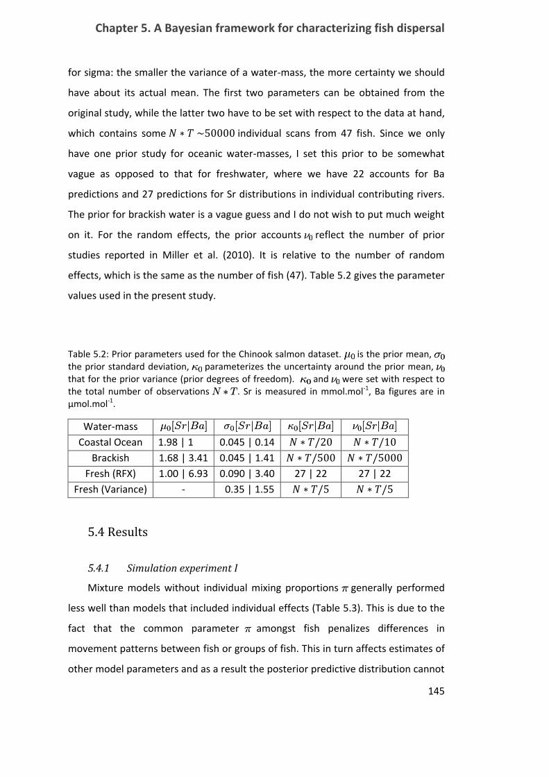
Chapter 5. A Bayesian framework for characterizing fish dispersal
145
for sigma: the smaller the variance of a water-mass, the more certainty we should
have about its actual mean. The first two parameters can be obtained from the
original study, while the latter two have to be set with respect to the data at hand,
which contains some individual scans from 47 fish. Since we only
have one prior study for oceanic water-masses, I set this prior to be somewhat
vague as opposed to that for freshwater, where we have 22 accounts for Ba
predictions and 27 predictions for Sr distributions in individual contributing rivers.
The prior for brackish water is a vague guess and I do not wish to put much weight
on it. For the random effects, the prior accounts º0º0 reflect the number of prior
studies reported in Miller et al. (2010). It is relative to the number of random
effects, which is the same as the number of fish (47). Table 5.2 gives the parameter
values used in the present study.
Table 5.2: Prior parameters used for the Chinook salmon dataset. ¹0¹0 is the prior mean, ¾0¾0 the prior standard deviation, ·0·0 parameterizes the uncertainty around the prior mean, º0º0 that for the prior variance (prior degrees of freedom). ·0·0 and º0º0 were set with respect to the total number of observations N ¤ TN ¤ T . Sr is measured in mmol.mol-1, Ba figures are in μmol.mol-1.
Water-mass ¹0[SrjBa]¹0[SrjBa] ¾0[SrjBa]¾0[SrjBa] ·0[SrjBa]·0[SrjBa] º0[SrjBa]º0[SrjBa]
Coastal Ocean 1.98 | 1 0.045 | 0.14
Brackish 1.68 | 3.41 0.045 | 1.41
Fresh (RFX) 1.00 | 6.93 0.090 | 3.40 27 | 22 27 | 22
Fresh (Variance) - 0.35 | 1.55
5.4 Results
5.4.1 Simulation experiment I
Mixture models without individual mixing proportions ¼¼ generally performed
less well than models that included individual effects (Table 5.3). This is due to the
fact that the common parameter ¼¼ amongst fish penalizes differences in
movement patterns between fish or groups of fish. This in turn affects estimates of
other model parameters and as a result the posterior predictive distribution cannot
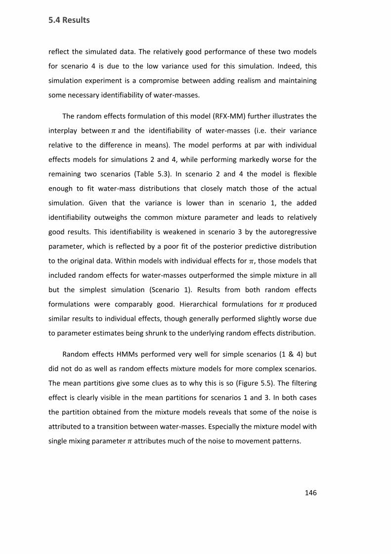
5.4 Results
146
reflect the simulated data. The relatively good performance of these two models
for scenario 4 is due to the low variance used for this simulation. Indeed, this
simulation experiment is a compromise between adding realism and maintaining
some necessary identifiability of water-masses.
The random effects formulation of this model (RFX-MM) further illustrates the
interplay between and the identifiability of water-masses (i.e. their variance
relative to the difference in means). The model performs at par with individual
effects models for simulations 2 and 4, while performing markedly worse for the
remaining two scenarios (Table 5.3). In scenario 2 and 4 the model is flexible
enough to fit water-mass distributions that closely match those of the actual
simulation. Given that the variance is lower than in scenario 1, the added
identifiability outweighs the common mixture parameter and leads to relatively
good results. This identifiability is weakened in scenario 3 by the autoregressive
parameter, which is reflected by a poor fit of the posterior predictive distribution
to the original data. Within models with individual effects for ¼¼, those models that
included random effects for water-masses outperformed the simple mixture in all
but the simplest simulation (Scenario 1). Results from both random effects
formulations were comparably good. Hierarchical formulations for produced
similar results to individual effects, though generally performed slightly worse due
to parameter estimates being shrunk to the underlying random effects distribution.
Random effects HMMs performed very well for simple scenarios (1 & 4) but
did not do as well as random effects mixture models for more complex scenarios.
The mean partitions give some clues as to why this is so (Figure 5.5). The filtering
effect is clearly visible in the mean partitions for scenarios 1 and 3. In both cases
the partition obtained from the mixture models reveals that some of the noise is
attributed to a transition between water-masses. Especially the mixture model with
single mixing parameter attributes much of the noise to movement patterns.

Chapter 5. A Bayesian framework for characterizing fish dispersal
147
Table 5.3: Simulation results for each scenario summarized the posterior predictive test
quantity E(¢Y )E(¢Y ) as well as by E(¢¼)E(¢¼) and the corresponding standard deviation sd(¢¼)sd(¢¼). E denotes the expectation in both cases. For both test quantities, lower absolute values for discrepancies between model posterior distributions and simulated data indicate better model fit. Model abbreviations are MM = mixture model, HMM = hidden Markov model, prefix RFX = random effects for water-masses, prefix DP = Dirichlet Process, suffix –I = individual ¼¼.
MM RFX-MM
MM-I RFX-
MM-I
DP-RFX-
MM-I
RFX-HMM
RFX-
HMM-I
Scenario E(¢Y )E(¢Y )
1 0.32 -0.21 0.027 ‐0.038 0.022 0.022 0.020
2 -0.17 -0.030 ‐0.14 ‐0.029 -0.030 -0.10 -0.067
3 -0.28 -0.42 ‐0.22 ‐0.065 0.027 -0.19 -0.14
4 -0.090 -0.047 ‐0.13 ‐0.020 -0.041 -0.035 -0.024
E(¢¼)[sd(¢¼)]E(¢¼)[sd(¢¼)]
1 - - ‐0.0018
[0.068]
‐0.0025
[0.068]
-0.0019
[0.068] - -
2 - - ‐0.17
[0.28]
‐0.0049
[0.086]
0.00042
[0.076] - -
3 - - ‐0.060
[0.47]
‐0.040
[0.084]
-0.0033
[0.088] - -
4 - - -0.24
[0.21]
-0.034
[0.086]
-0.0026
[0.068] - -
The HMMs clearly give a better approximation of the true partition for
scenario 1: The noisy observations rarely contribute to changes in the (filtered)
sequence of environments (Figure 5.5). Scenario 3 however demonstrates a
drawback of this filtering in difficult situations. When the true parameters are hard
to estimate, the estimated partition may be substantially different form the true
partition. Strong constraints on the transition probabilities (see considerations
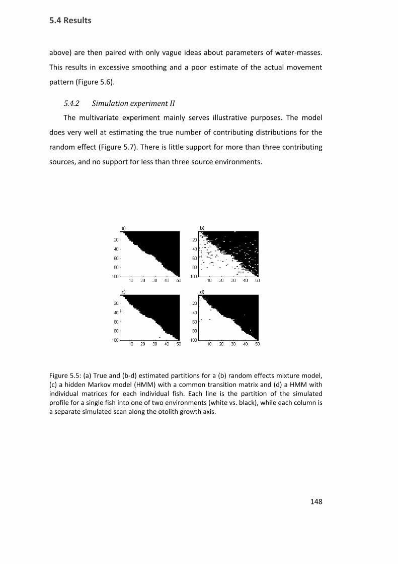
5.4 Results
148
above) are then paired with only vague ideas about parameters of water-masses.
This results in excessive smoothing and a poor estimate of the actual movement
pattern (Figure 5.6).
5.4.2 Simulation experiment II
The multivariate experiment mainly serves illustrative purposes. The model
does very well at estimating the true number of contributing distributions for the
random effect (Figure 5.7). There is little support for more than three contributing
sources, and no support for less than three source environments.
Figure 5.5: (a) True and (b-d) estimated partitions for a (b) random effects mixture model, (c) a hidden Markov model (HMM) with a common transition matrix and (d) a HMM with individual matrices for each individual fish. Each line is the partition of the simulated profile for a single fish into one of two environments (white vs. black), while each column is a separate simulated scan along the otolith growth axis.
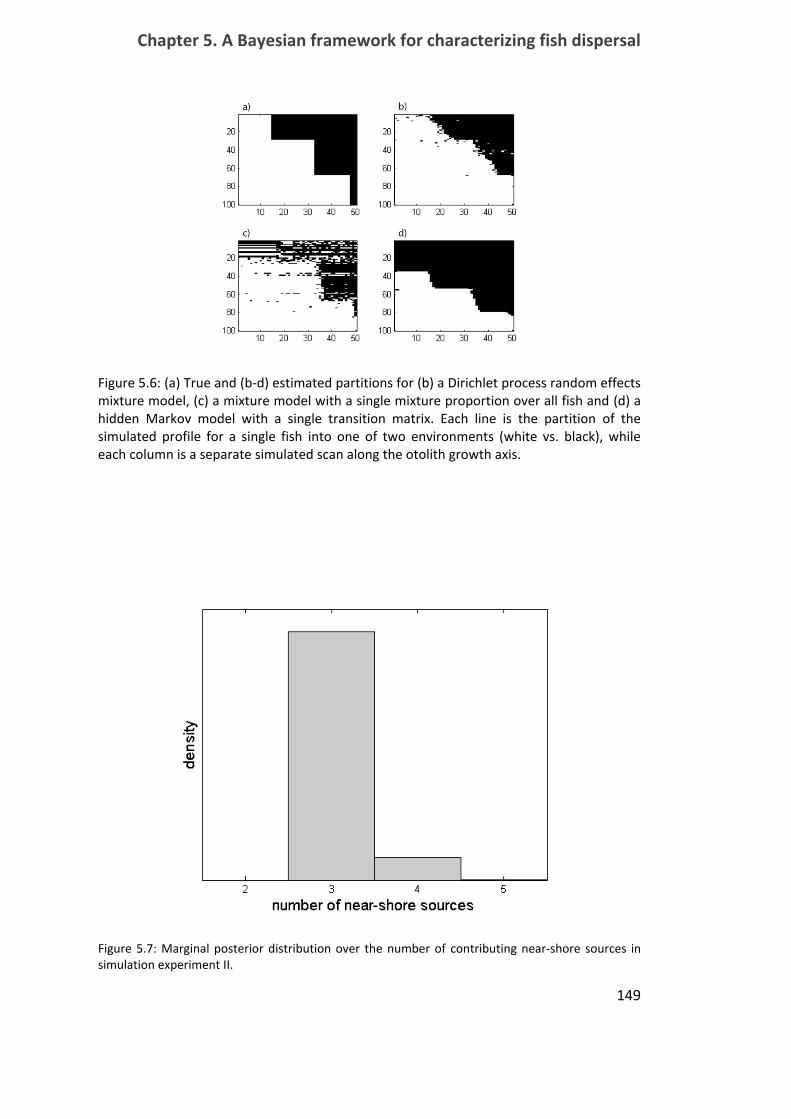
Chapter 5. A Bayesian framework for characterizing fish dispersal
149
Figure 5.6: (a) True and (b-d) estimated partitions for (b) a Dirichlet process random effects mixture model, (c) a mixture model with a single mixture proportion over all fish and (d) a hidden Markov model with a single transition matrix. Each line is the partition of the simulated profile for a single fish into one of two environments (white vs. black), while each column is a separate simulated scan along the otolith growth axis.
Figure 5.7: Marginal posterior distribution over the number of contributing near-shore sources in simulation experiment II.
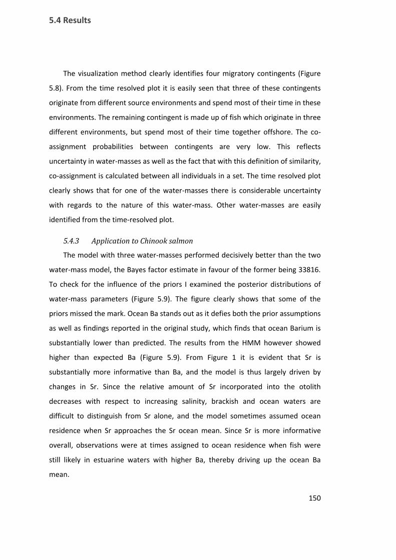
5.4 Results
150
The visualization method clearly identifies four migratory contingents (Figure
5.8). From the time resolved plot it is easily seen that three of these contingents
originate from different source environments and spend most of their time in these
environments. The remaining contingent is made up of fish which originate in three
different environments, but spend most of their time together offshore. The co-
assignment probabilities between contingents are very low. This reflects
uncertainty in water-masses as well as the fact that with this definition of similarity,
co-assignment is calculated between all individuals in a set. The time resolved plot
clearly shows that for one of the water-masses there is considerable uncertainty
with regards to the nature of this water-mass. Other water-masses are easily
identified from the time-resolved plot.
5.4.3 Application to Chinook salmon
The model with three water-masses performed decisively better than the two
water-mass model, the Bayes factor estimate in favour of the former being 33816.
To check for the influence of the priors I examined the posterior distributions of
water-mass parameters (Figure 5.9). The figure clearly shows that some of the
priors missed the mark. Ocean Ba stands out as it defies both the prior assumptions
as well as findings reported in the original study, which finds that ocean Barium is
substantially lower than predicted. The results from the HMM however showed
higher than expected Ba (Figure 5.9). From Figure 1 it is evident that Sr is
substantially more informative than Ba, and the model is thus largely driven by
changes in Sr. Since the relative amount of Sr incorporated into the otolith
decreases with respect to increasing salinity, brackish and ocean waters are
difficult to distinguish from Sr alone, and the model sometimes assumed ocean
residence when Sr approaches the Sr ocean mean. Since Sr is more informative
overall, observations were at times assigned to ocean residence when fish were
still likely in estuarine waters with higher Ba, thereby driving up the ocean Ba
mean.

151
Figure 5.8: Visualization of marginal similarity of transects from simulation experiment II. a) The tree displays average marginal similarity: Co-assignment probabilities (node heights in the tree) are marginal over the i) estimated number of water-masses and ii) parameter uncertainty. b) The time resolved plot shows the marginal number of fish in the same water mass as fish i at time t, identical shades of grey thus indicate common dispersal paths for a given group identified from the tree. c) The true partition including the three different contributing random effects sources, visible as like shades of grey.
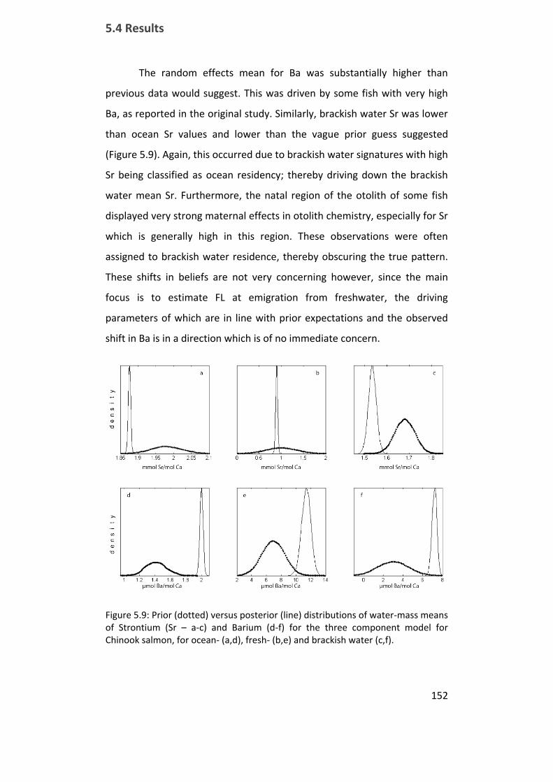
5.4 Results
152
The random effects mean for Ba was substantially higher than
previous data would suggest. This was driven by some fish with very high
Ba, as reported in the original study. Similarly, brackish water Sr was lower
than ocean Sr values and lower than the vague prior guess suggested
(Figure 5.9). Again, this occurred due to brackish water signatures with high
Sr being classified as ocean residency; thereby driving down the brackish
water mean Sr. Furthermore, the natal region of the otolith of some fish
displayed very strong maternal effects in otolith chemistry, especially for Sr
which is generally high in this region. These observations were often
assigned to brackish water residence, thereby obscuring the true pattern.
These shifts in beliefs are not very concerning however, since the main
focus is to estimate FL at emigration from freshwater, the driving
parameters of which are in line with prior expectations and the observed
shift in Ba is in a direction which is of no immediate concern.
Figure 5.9: Prior (dotted) versus posterior (line) distributions of water-mass means of Strontium (Sr – a-c) and Barium (d-f) for the three component model for Chinook salmon, for ocean- (a,d), fresh- (b,e) and brackish water (c,f).
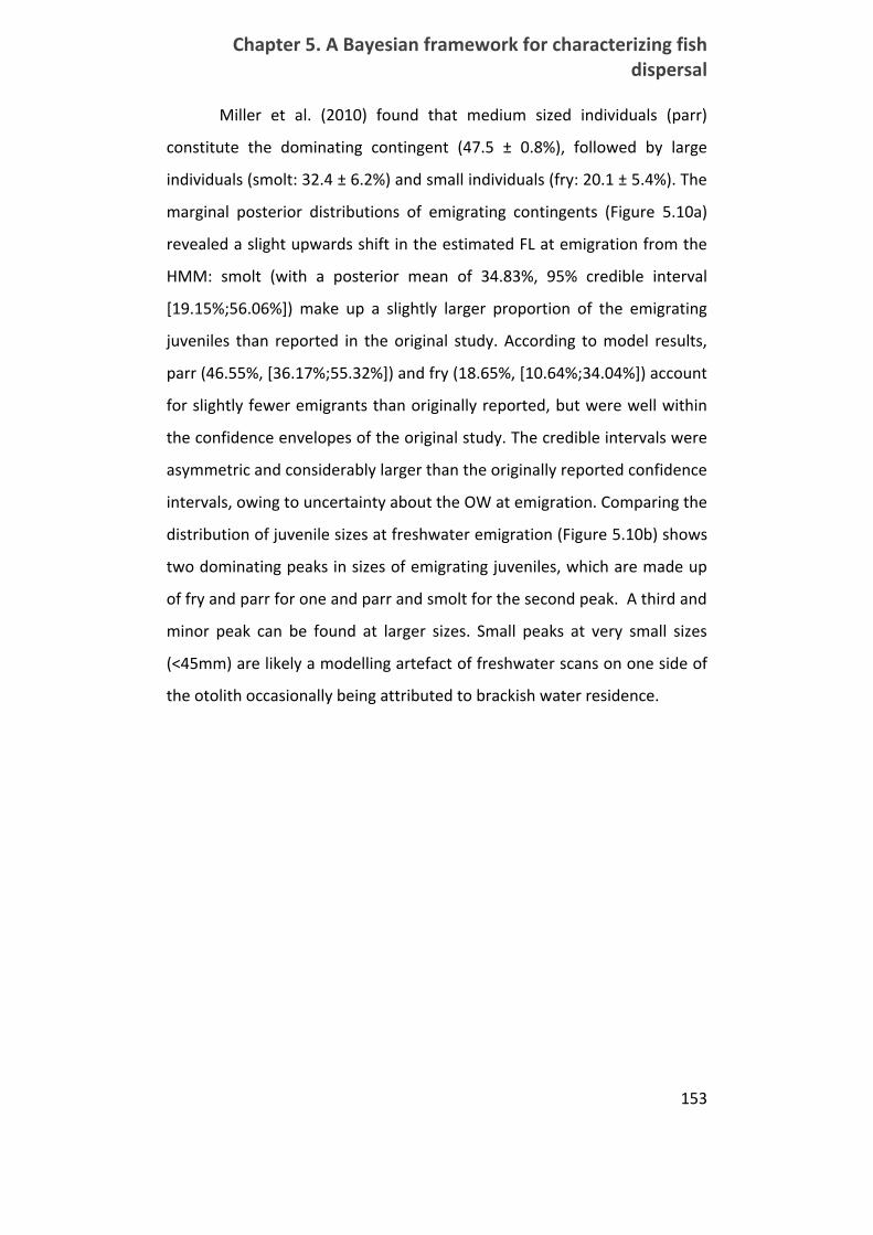
Chapter 5. A Bayesian framework for characterizing fish dispersal
153
Miller et al. (2010) found that medium sized individuals (parr)
constitute the dominating contingent (47.5 ± 0.8%), followed by large
individuals (smolt: 32.4 ± 6.2%) and small individuals (fry: 20.1 ± 5.4%). The
marginal posterior distributions of emigrating contingents (Figure 5.10a)
revealed a slight upwards shift in the estimated FL at emigration from the
HMM: smolt (with a posterior mean of 34.83%, 95% credible interval
[19.15%;56.06%]) make up a slightly larger proportion of the emigrating
juveniles than reported in the original study. According to model results,
parr (46.55%, [36.17%;55.32%]) and fry (18.65%, [10.64%;34.04%]) account
for slightly fewer emigrants than originally reported, but were well within
the confidence envelopes of the original study. The credible intervals were
asymmetric and considerably larger than the originally reported confidence
intervals, owing to uncertainty about the OW at emigration. Comparing the
distribution of juvenile sizes at freshwater emigration (Figure 5.10b) shows
two dominating peaks in sizes of emigrating juveniles, which are made up
of fry and parr for one and parr and smolt for the second peak. A third and
minor peak can be found at larger sizes. Small peaks at very small sizes
(<45mm) are likely a modelling artefact of freshwater scans on one side of
the otolith occasionally being attributed to brackish water residence.
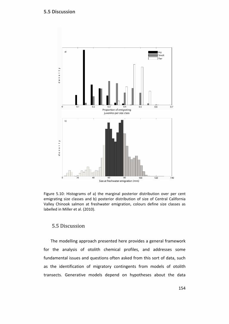
5.5 Discussion
154
Figure 5.10: Histograms of a) the marginal posterior distribution over per cent emigrating size classes and b) posterior distribution of size of Central California Valley Chinook salmon at freshwater emigration, colours define size classes as labelled in Miller et al. (2010).
5.5 Discussion
The modelling approach presented here provides a general framework
for the analysis of otolith chemical profiles, and addresses some
fundamental issues and questions often asked from this sort of data, such
as the identification of migratory contingents from models of otolith
transects. Generative models depend on hypotheses about the data

Chapter 5. A Bayesian framework for characterizing fish dispersal
155
generating mechanism. In the case of chemical transects across otoliths,
one needs to specify hypotheses about water-masses that could be
reflected within these transects. Often, strong prior information is available
about patterns (such as for Ba and Sr) which we can exploit (i.e. Elsdon &
Gillanders 2003, Fablet et al. 2007). In other cases however, the observed
patterns cannot be a priori tied to a known number of environments (i.e.
Shima & Swearer 2009a). In this case the present framework can be used
to compare competing models about different potential hypotheses about
dispersal or infer the number of distinct water masses directly using the DP
extension. Thus, while specifying a specific generative mechanism may be
difficult at times, these models can still provide insight about a likely
generating mechanism. I also found that it helps to plot the global
frequency distribution of the data along with the actual transects when
thinking about such hypotheses (i.e. Figure 5.1). The underlying hypotheses
of these models are verifiable, and beliefs about models and their
parameters can be updated in the light of further studies which test
underling hypotheses. Furthermore, credible intervals for each model
parameter provide us with an idea of how much the inferences from each
model are worth. For models that produced poor results in the simulations,
I could generally observe that some parameters, such as random effects for
instance, had absurdly large credible intervals.
In order to construct generative models and specify their distributions
over water-masses, the meaning of water-masses or environments needs
to be clearly defined. Most importantly, these need to be identifiable from
the data. Having an idea of the scales over which (otolith-, and ideally
water-) chemistries change is thus indispensible (Elsdon et al. 2008). Prior
assumptions about such scales through prior distributions on water-mass
variances can be a way to explicitly define the scale on which to consider a
water-mass. In the Chinook example I place an informative prior on the
variance of the water-masses, which are thereby defined to be ‘within
5.5 Discussion
156
river’ for freshwater signatures for example. While the Dirichlet Process
models aim to estimate the number of water-masses in a given dataset,
the same consideration applies: we can only identify the number of distinct
environments in the model if these are identifiable in the first place, or if
we know the scale of variation of individual water-mass signatures.
The application to Chinook salmon illustrates the merit and validity of
the Bayesian approach, but also some possible pitfalls. The posterior
distributions for emigration percentages for the three size classes provide a
way to assess uncertainty in estimates of freshwater residence:
distributions over the percentage of emigrating fry and parr for instance
are highly skewed and the posterior mode may provide a better estimate
of the true percentage per size class than does the mean. Miller et al.
(2010) used thresholds to visually define the transition between habitats.
While transitions are relatively clear for most fish, they are rather smooth
for some. The definition of this threshold thus clearly presents a degree of
subjectivity, which introduces uncertainty in the actual otolith width at
emigration. The Bayesian model integrates over this uncertainty, which is
evident in considerably larger credible intervals.
One needs to be cautious however in directly interpreting water-mass
distributions: the analysis shows that transitional periods and maternal
effects can influence these estimates. It is thus likely that any smooth
transitions in salinity for instance will somewhat effect other parameters of
interest. This may be in part the reason why I observe a slight shift in FL at
emigration, and hence in relative percentages of emigrating juveniles for
the tree size classes. My estimates are very close to the original estimates
however and represent a shift of only one individual per category.
Furthermore, simulation scenario 4 indicates that most realistic models
perform well even in the presence of transitional zones.

Chapter 5. A Bayesian framework for characterizing fish dispersal
157
One of the most important applications of the methods presented here
is the identification of migratory contingents. The definition of a contingent
is dependent on the number of environments considered as well as the
parameters of interest in a particular study. Secor (1999) for instance
defines a contingent as “ …a level of fish aggregation based upon divergent
migratory behaviours or habitat use within a population,…”. In the Chinook
salmon example these contingents would be fish that spend comparable
time in their natal freshwater habitat, but alternative contingents could be
fish that spend comparable time in fresh- and brackish water. Using this
objective method produces two dominant peaks in the distribution over
size at emigration, which may be two main emigrating contingents, each
containing individuals from two of the pre-defined size classes (fry & parr
or parr & smolt respectively). The histogram in (Figure 6a) in Miller et al.
(2010) shows a shape which resembles a normal distribution, but this
difference may be due to the larger bin size for the histogram in the
original study.
The marginal descriptions of the model outputs illustrate the advantage
of a fully Bayesian approach: it opens the possibility to define contingents
and similarity of dispersal syndromes which integrate over unknown
parameters and thereby provide robust descriptions of fish migrations. This
approach assumes that the belief that two fish shared a similar dispersal
history is lower the more uncertain we are about the number and nature of
different water-masses, and hence about a fishes migration history.
Uncertainty about water-masses is only present in DP-random effects
models, but effects our beliefs in co-assignment probabilities significantly.
This definition of similarity makes intuitive sense: the more certain we are
about the data generating mechanism and the underlying parameters, the
more sure we can be about a fish’s dispersal history. Note that this
approach is rather different from what researchers often use for this sort
of data: A repeated measure ANOVA, for instance, will test for difference

5.5 Discussion
158
between transects, and migration histories are regarded as not-separable
when no significant difference is found. The approach presented here aims
to infer similarity: dissimilarity is thus the ‘default’ and is higher the more
uncertainty is represented in the posterior distribution.
One drawback of this marginal method for finding contingents is that it
relies on fish profiles being aligned i.e. scans should correspond to the
same age or be aligned to correspond. This is the case when profiles run
from the otolith core, often identifiable by a distinct peak in Manganese
and other elements (Brophy et al. 2004, Ruttenberg et al. 2005), to the
edge. For profiles of different lengths, the marginal (the number of fish
in the same environment as fish i at time t) can be adjusted to account for
the number of fish still aligned at time t. For profiles spanning the entire
otoliths such as in the salmon example, an alignment based on a peak in
Mn for instance can still be made if the location of that peak has been
identified. Alignment is difficult otherwise, and one has to resort to
multiple alignment algorithms.
The Bayesian approach proposed in this study opens the door to more
complex analyses. It allows not only for added flexibility, but also for
simultaneous estimation of all relevant parameters, which ensures that
uncertainty in parameters is handled appropriately. For example, I already
mentioned above that it would be possible to integrate other data sources
which may specify relationships between water chemistry and otolith
chemistry, and allow for the reconstruction of specific dispersal pathways
(Royer et al. 2005). The inclusion of prior beliefs about water-mass
characteristics provides a way to incorporate knowledge of patterns in
otolith chemistry. The model for the Chinook data demonstrates how shifts
in belief about such parameters can happen even when drawing on a body
of prior studies to define prior distributions.
Chapter 5. A Bayesian framework for characterizing fish dispersal
159
An automated approach can provide advantages such as
standardization amongst different studies and the elimination of subjective
thresholds and decisions (Fablet et al. 2007, Hedger et al. 2008). The
framework proposed here however goes beyond a simple analysis of
habitat sequences. The extensions I propose are but some simple additions
to these models. Recent advances in movement ecology highlight the
potential of latent state models (Patterson et al. 2008, Schick et al. 2008,
Patterson et al. 2009). In particular, generative hierarchical models can
contribute significantly to mechanistic understandings of animal movement
(Schick et al. 2008).
Larval dispersal in the marine environment can, for instance, be
influenced by strong selective forces, which are thought to increase under
fishing and habitat fragmentation (Baskett et al. 2007). The models
presented here could be used to study inert versus environmentally driven
movements. The relative contribution of these two components of
dispersal can have important consequences for metapopulation dynamics
(Secor 1999, Clobert et al. 2009, Hawkes 2009), especially if heritable
components of movements vary on short time-scales (Hawkes 2009). The
transition matrix in an HMM can be interpreted as a habitat preference
model for adult fish which actively choose habitats, or as a model for
favourable conditions (whether actively chosen or not) for larval fish.
Hierarchical and regression formulations within a hierarchical framework
for underlying parameters could then help identify individual variation as
opposed to inert behaviour and further relate these to individual condition
or fitness. Otolith chemistry, in conjunction with other data, such as that
issued from otolith structural analysis, can provide significant insights into
the ecology of fish (Campana & Thorrold 2001). I provide a structural
framework that gives a probabilistic basis to analyse such complex data
coherently.

5.5 Discussion
160
161
Chapter 6
6. Inshore residency of fish larvae may maintain
connections in a reef fish metapopulation
6.1 Introduction
The lifecycle of most marine organisms displays a dispersive and
elusive larval stage, which makes direct observation of dispersal between
populations difficult and hinders efforts to predict dynamics of spatially
structured populations. Despite an increasing number of studies, our
knowledge of the relative importance of processes that govern larval
dispersal remains limited. It is evident that larvae can, at least locally,
determine the outcome of the dispersal process through behaviour and
plasticity in their development (Bradbury et al. 2003, Lecchini 2005, Fiksen
et al. 2007, Leis 2007, Morgan & Anastasia 2008, Morgan & Fisher 2010).
The dynamic ocean environment through which larvae disperse may also
play a predominant role by not only determining dispersal outcomes, but
also adaptations of dispersing larvae to this environment (Armsworth et al.
2001, Strathmann et al. 2002, Largier 2003, Siegel et al. 2003, Shanks &
Eckert 2005, Byers & Pringle 2006).
Many marine organisms must persist in advective environments,
where the mean flow is unidirectional (Shanks & Eckert 2005). In such
environments, local hydrodynamic conditions are pivotal for the
maintenance of populations at the upstream limit of the species: without
6.1 Introduction
162
such mechanisms, populations would drift downstream and eventually go
extinct (Swearer et al. 2002, Largier 2003, Byers & Pringle 2006).
Hydrodynamic conditions may therefore act as an important evolutionary
driver of strategies to avoid advection and the associated uncertainty of
returning to favourable settlement habitat (Strathmann et al. 2002, Shanks
& Eckert 2005). The successful self‐recruitment of larvae to (or upstream
of) their natal habitat depends on the relative strength of mean advective
currents and the larval strategies to counter such advective forces
(Armsworth 2001, Armsworth et al. 2001, Fisher 2005, Byers & Pringle
2006). Larval behaviour may be particularly effective in that respect by
allowing larvae to exploit retention features (Breitburg et al. 1995, Morgan
& Fisher 2010) or locally developing counter-currents (Paris & Cowen
2004).
While the potential importance of such strategies for the maintenance
of metapopulations and reserve networks is evident from theoretical
models (White et al. 2010), the degree to which these strategies prevail on
the scale of a metapopulation network is unknown. If adaptations to avoid
advective forces dominate the dispersal process, we should find species-
specific patterns of dispersal across the system, which could be reflected in
common dispersal histories (i.e. adaptations for dispersal which cause the
majority of larvae to migrate offshore (Morgan & Anastasia 2008)). If, on
the other hand, local hydrodynamic conditions determine dispersal
histories, we would expect the dispersal histories of fish settling to differ
according to site-specific conditions. By examining dispersal histories of
settling fish in a number of local populations we may gain insight about the
relative importance of drivers of dispersal patterns within a system.
Fish otoliths (ear‐bones) have become an essential tool for fish
biologists, allowing insights into dispersal histories in a variety of situations
(Thorrold et al. 2002, Elsdon et al. 2008). In particular, the concentric
Chapter 6. Inshore residency of fish larvae may maintain connections in a reef fish metapopulation
163
growth and continued deposition of minerals during a fish’s life make the
otolith an ideal tool to study dispersal and migration: it acts as a ‘flight
recorder’, continuously including trace elements that reflect environmental
conditions (Campana 1999, Elsdon et al. 2008). Distinct chemical and visual
marks in the otolith microstructure are furthermore associated with
settlement and metamorphosis in some fish, facilitating identification of
pelagic larval duration (PLD), settlement events and related metrics (Hale &
Swearer 2008, Hamilton & Warner 2009).
Motivated by the seemingly contradictory result of upstream dispersal
found in chapter 4, this chapter investigates dispersal histories of these
Forsterygion lapillum recruits as evidenced by otolith chemistry. Describing
dispersal histories from a series of chemical measurements is an active
area of research and a number of statistical methods have recently been
proposed to infer offshore transport (Sandin et al. 2005, Hamilton et al.
2008), describe habitat shifts (Fablet et al. 2007) or uncover patters from
time‐series of chemical measurements (or profiles / transects) across
otoliths (Shima & Swearer 2009a). In this chapter I build on the methods
developed in chapter 5 to develop a flexible Bayesian model of larval
dispersal in Cook Strait. I use a Bayesian mixture model that infers inshore
residency from transects of chemical measurements across the recruit
otoliths. Different wind-generated flow regimes simulated within the
hydrodynamic model developed in chapter 4 provide insight into the
potential benefit of inferred dispersal histories. I specifically aim to answer
the following questions: i) given the hypothesis of two distinct water
masses (’inshore and ’offshore’), do common triplefin larvae in Cook Strait
disperse in offshore or nearshore waters? ii) Are these dispersal history
patterns common to fish sampled throughout the system and iii) could
these patterns be related to local hydrodynamics?

6.2 Methods
164
6.2 Methods
6.2.1 Recruit otolith preparation and pre‐processing
I investigated the dispersal history of F. lapillum recruits in three
marine reserve sites (collected for chapter 4) using chemical profiles (time
series of individual chemical scans) across otoliths. Chemical analysis of
recruit otoliths followed methods described in Shima & Swearer (2009a).
Briefly, I used Laser Ablation Inductively Coupled Mass Spectrometry (LA‐
ICPMS) to sample material corresponding to the dispersive larval phase of
recruits. Transects were ablated using a 80x5μm rectangular spot which
was moved across the post‐rostral axis of the otolith at constant speed
(3μm/s). This produced a time series of elements across the otolith from
just outside the natal (core) region to the most recently deposited material
(i.e. the settlement mark). I determined the length of the transects visually
by stopping transects at the settlement mark, which is visible in this species
(Kohn 2007, Shima & Swearer 2009a). I further used Barium as a chemical
indicator of the settlement mark to guide this process (Hale & Swearer
2008, Hamilton & Warner 2009).
6.2.2 Statistical model
To characterize dispersal histories of recruits, I formulate a model that
distinguishes inshore residence and offshore dispersal of larvae. The
central assumption underlying this model and its interpretation is that
some recruits will experience chemically distinguishable inshore and
offshore waters. Inshore waters for instance may be water masses near a
recruit’s spawning location: F. lapillum spawns in sheltered locations close
to shore, providing an empirical motivation for this assumption. I further
assume that ontogenetic effects and differences in growth rate will have a
negligible effect on overall patterns inferred by these models.
I start with the assumption that offshore water masses are usually
depleted in some trace elements relative to inshore or estuarine waters.
Chapter 6. Inshore residency of fish larvae may maintain connections in a reef fish metapopulation
165
These waters may thus produce distinct chemical signatures in the otolith
(this may not be the case for all elements or in regions of strong upwelling
(Elsdon et al. 2008)). I restrict the elemental analysis to Barium, though
other elements could be used and a multivariate extension of the method
is straightforward. Barium to Calcium ratios in otoliths have been shown to
be influenced by environmental concentrations (Walther & Thorrold 2006),
and are usually lower in oceanic waters relative to inshore waters (Elsdon
& Gillanders 2005, Elsdon et al. 2008, Hamilton et al. 2008). An example of
Barium traces across F. lapillum recruit otoliths is shown in Figure 6.1.
At the most basic level, I model the Barium time series
y = yi;1; : : : ; yi;t; : : : ; yi;Ty = yi;1; : : : ; yi;t; : : : ; yi;T of TT scans along the otolith of recruit ii as a
mixture (a weighted sum) of KK normal distributions pertaining to the same
number of potential source environments (Figure 6.1), each with different
means ¹=¹1:::¹k:::¹K¹=¹1:::¹k:::¹K and potentially unique standard deviations
¾=¾1:::¾k:::¾K¾=¾1:::¾k:::¾K. For i=1:::Ni=1:::N fish the joint density is thus:
f(yj¼;¹;¾2) =
NY
i=1
TY
t=1
KX
k=1
¼i;kf(yi;tj¹k;¾2k)f(yj¼;¹;¾2) =
NY
i=1
TY
t=1
KX
k=1
¼i;kf(yi;tj¹k;¾2k)
with ff denoting the normal density. ¼ = (¼i; 1:::¼i; k:::¼i; K)¼ = (¼i; 1:::¼i; k:::¼i; K) and
¼ = (¼1:::¼i:::¼N )¼ = (¼1:::¼i:::¼N ) then denote the vector over all source proportions for
individual ii, and the set of vectors of source proportions for all individuals,
respectively. It is convenient to think of the ¼i;k¼i;k as mixture proportions for
the mixture components - 2 in this case, representing near‐shore and
offshore water masses.
For treatment in a Bayesian hierarchical sense, I re‐write the model in
terms of (latent) class indicator variables »i;t»i;t that assign the tt ‐th
observation of the ii‐th recruit to the kk‐th water mass:

6.2 Methods
166
yi;tj¹;¾2; »i;t » N(¹1 + »i;t¹2;¾
2(1+»i;t)
)
»i;tj¼i » Bernoulli(¼i)
¼i;k » Beta(1=K)
yi;tj¹;¾2; »i;t » N(¹1 + »i;t¹2;¾
2(1+»i;t)
)
»i;tj¼i » Bernoulli(¼i)
¼i;k » Beta(1=K)
In its simplest form, this model will assign observations to one of two
distributions, where ¹1¹1 is the mean of the offshore Barium signatures and
¹1 + ¹2¹1 + ¹2 is the mean of near‐shore water masses (the additive formulation
together with a restriction for ¹2¹2 to be positive is used for identifiability of
the mixture indicators »», as their labels would otherwise lose their meaning
during estimation). »i;t»i;t is thus either 0 for offshore or 1 for nearshore water
masses and fish spend a proportion ¼k¼k of their larval duration in
environment kk. This initial setup is similar to previous studies in terms of
assumptions (Sandin et al. 2005, Hamilton et al. 2008) and model
formulation (Fablet et al. 2007).
Figure 6.1: a) Example of three 138Ba:Ca traces in mol.(mol Ca)-1 x10⁻⁶ and b) resulting density estimates. Density outlines correspond to line types of the Ba traces; colours were added for ease of visualization of the densities. These densities are the basis of the mixture model which treats each transect as a mixture of two normal densities, one modelling near‐shore water masses and the other modelling offshore water masses.
Many studies have used otolith chemistry for near‐shore‐ and/or
estuarine fish to distinguish natal regions (Warner et al. 2005, Barbee &
Swearer 2007, Ruttenberg et al. 2008, Standish et al. 2008, Fontes et al.
Chapter 6. Inshore residency of fish larvae may maintain connections in a reef fish metapopulation
167
2009, Neubauer et al. 2010). Estuaries may, for instance, have significantly
higher Barium loads than coastal waters (Elsdon & Gillanders 2005, Miller
et al. 2010), which will in turn result in substantially higher Barium
concentration for estuarine spawned individuals during their early life
history. In terms of the above model, retention for some coastally spawned
fish could then be under-estimated by falsely designating coastal inshore
signatures as reflections of offshore water masses (see for instance the
simulations in chapter 5). To incorporate the fact that different natal
regions will produce different near‐shore signatures, I extended this initial
model to include individual random effects at this level:
yi;tj¹;¾2; »i;t » N(¹1 + »i;t¹i;2;¾
2(1+»i;t)
)
log(¹i;2) » N(º; ¿ 2)
»i;tj¼i » Bernoulli(¼i)
¼i;k » Beta(1=K)
yi;tj¹;¾2; »i;t » N(¹1 + »i;t¹i;2;¾
2(1+»i;t)
)
log(¹i;2) » N(º; ¿ 2)
»i;tj¼i » Bernoulli(¼i)
¼i;k » Beta(1=K)
The logarithm in this formulation of the random effect assures that near‐
shore water masses produce higher Ba signatures and makes the mixture
identifiable. Priors for all quantities are vague.
Comparison of estimated values between sites may shed light on
factors that govern dispersal in this system. For each site I calculated the
posterior distribution of ¼i2¼i2 , the proportion of time spent inshore by recruit
ii. For models applied independently to the three reserves, I also calculated
the modal dispersal histories from the posterior distribution of »» .
Randomization tests were used to compare the pelagic larval duration
(PLD) of recruits, expectations of retention proportions (the expected value
of ¼2¼2) as well as total time dispersed ¿ =¼1 ¤PLD¿ =¼1 ¤PLD amongst locations. I
further investigated whether time spent offshore predicts the PLD. I again
used randomization to assess significance of the regression coefficients
that relate these two metrics. To verify that initial Ba did not account for
the observed patterns in inshore vs. offshore residence (i.e. a strong
6.2 Methods
168
ontogenetic signal) I used regression of maximum Ba concentrations for
fish against ¼2¼2.
All results are based on 10000 samples from the posterior distribution
after discarding the initial 1000 iterations for every Markov Chain (the
burn-in). The resulting sequences of draws were inspected for
autocorrelation and convergence. I tested whether the chains were
sensitive to initial conditions by running the MCMC repeatedly for
randomly generated initial values for parameters.
6.2.3 Hydrodynamic model investigation
In this chapter I again used an implementation of the Gerris flow-
solver ocean model (outlined in Chapter 4) to investigate different flow
patterns that may have developed during the period of investigation,
namely from mid-December to early March 2008. I specifically studied
differences in flow regimes induced by wind regimes, which are likely the
driving force for local variation about the mean current (Heath 1986,
Chiswell & Stevens 2010). Such variation could be exploited by larvae of
nearshore species to avoid advection in mean currents in order to stay near
favourable habitats [Morgan, 2010 #3562]. Two wind directions, northerly
and southerly winds, make up the majority of observed winds in in Cook
Strait (Figure 6.2). Recent empirical observations indicate that these winds
can have a strong effect on dispersal of passive drifters in the vicinity of
Kapiti Island (Chiswell & Stevens 2010). Strong southerly winds can, for
instance, drive drifter retention in Kapiti Island and may be enough to
counter the mean flow induced by the d’Urville current.
I used information from regional wind records (obtained from the New
Zealand National Climate Database at http://cliflo.niwa.co.nz/) to
investigate wind regimes and corresponding flow patterns in the Strait.
Winds were predominantly from the north (Figure 6.2a), but some
prolonged southerly events also happened during the period 2 month

Chapter 6. Inshore residency of fish larvae may maintain connections in a reef fish metapopulation
169
period of this study (Figure 6.2b). I modelled distinct wind events
comparable to those found during the time of our study as time averaged
northerlies and southerlies which were compared against each other.
Simulations were conducted over 2 and 5 day intervals, which is close to
the mode and maximum of southerly wind event durations. I compared
residual flow (by subtracting the tidal component of the flow from
simulations) in the region between northerly and southerly regimes. Since
empirical results where most intriguing for North Island populations, and
because the effects of wind driven transport is easier to appreciate and
visualize on a simple coastline, I concentrated this investigation on the
stretch of coastline between Kapiti Island and Wellington. Gerris was
allowed to refine the coastal topography and to adapt to flow patterns up
to a maximum resolution of 117.19m in this region, while keeping the
resolution in the rest of Cook Strait at 3.5km.
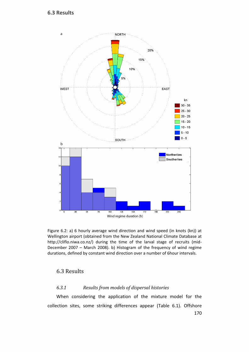
6.3 Results
170
Figure 6.2: a) 6 hourly average wind direction and wind speed (in knots (kn)) at Wellington airport (obtained from the New Zealand National Climate Database at http://cliflo.niwa.co.nz/) during the time of the larval stage of recruits (mid-December 2007 – March 2008). b) Histogram of the frequency of wind regime durations, defined by constant wind direction over a number of 6hour intervals.
6.3 Results
6.3.1 Results from models of dispersal histories
When considering the application of the mixture model for the
collection sites, some striking differences appear (Table 6.1). Offshore

Chapter 6. Inshore residency of fish larvae may maintain connections in a reef fish metapopulation
171
means (¹1¹1) are considerably higher in Long Island relative to Wellington
and Kapiti offshore signatures. Differences between mean inshore (log(º)log(º))
and offshore signatures are also greatest at Long Island, whereas recruits
at Kapiti show the most subtle changes in Ba. Signatures are also the least
variable in Kapiti, whereas both inshore means and their variance are
substantially higher in Long Island, and to a lesser degree in Wellington.
Offshore means are rather similar between Kapiti and Wellington recruits;
however the variance about this mean is considerably higher in Wellington.
The variance around individual inshore means is indistinguishable between
the two sites but the variance about the random effects mean is
considerably higher in Wellington, owing to the large spread in inshore
signatures between self-recruited individuals, presumably from Wellington
harbour (c.f. chapter 4), and dispersed individuals from Kapiti (see results
below).
Table 6.1: Expected values and 95 per cent credible interval (in square brackets) of the posterior distribution of some parameters in the dispersal model. Values are in mol Ba. mol Ca-1 (x10-6). ¹1¹1 designates the offshore water-mass mean, ¾2
1¾21 its
variance. The variance in of individual water masses is given by ¾22¾22. The mean of
the random effect for near-shore water-masses is given by ¹1 + log(º)¹1 + log(º) with
associated variance & 2& 2 for the random effect.
Site ¹1¹1 log(º)log(º) ¾21¾21 ¾2
2¾22 & 2& 2
Kapiti 1.18
[1.16;1.20]
2.03
[1.73;2.34]
0.52
[0.50;0.54]
0.16
[0.14;0.17]
0.47
[0.24;0.91]
Island
Bay
1.07
[1.06;1.09]
3.29
[2.38;4.19]
2.07
[2.00;2.14]
0.16
[0.15;0.17]
4.85
[2.56;9.20]
Long
Island
5.62
[5.48;5.75]
6.56
[3.87;9.23]
4.60
[4.37;4.83]
9.76
[8.93;10.57]
40.69
[20.33;80.25]
Dispersal patterns are similar at all sites, showing substantial
propositions of retention signatures for earlier parts of the PLD of most
larvae (Figure 6.3). The posterior expectation for the retention proportion

6.3 Results
172
¼2¼2 ranged from 0.41 to 0.98 in Kapiti (Figure 6.3a), from 0.02 to 0.98 in
Island Bay (Figure 6.3b) and from 0.26 to 0.99 in Long Island (Figure 6.3c).
Only in Island Bay do I find four larvae whose dispersal history indicates
that they likely spent all of their larval life in waters masses characterized
as offshore. This seems to be the case for only one recruit in Long Island
and none in Kapiti Island.
When comparing dispersal histories to predicted self-recruitment
patterns (see chapter 4), results suggest that most self-recruited fish were
retained inshore for the majority or all of their PLD. These results are
further consistent with the hypothesis that retained individuals in Long
Island were retained within the Sound for their entire PLD (Figure 6.3c). A
similar pattern is evidenced for fish that were regionally self-recruited in
Island Bay: I hypothesized that most of these fish likely came from within
the harbour in Wellington (c.f. chapter 4), and dispersal histories are
consistent with this hypothesis. Model results suggest that many of them
appear to have spent the majority of their PLD within Wellington Harbour,
or surrounding bays, before recruiting to the nearby open coast (Figure
6.3b). Some, however, appear to have been flushed out of the harbour
earlier, yet they still recruited close to their natal region. The dispersal
model also predicts that recruits at Kapiti likely spent most of their PLD
inshore, though one individual appears to have left inshore waters for
offshore waters before recruiting back to the natal region (Figure 6.3a).
The Pelagic larval duration is not significantly different amongst any of
the locations (Table 6.2). Time and proportion of PLD spent nearshore is
higher at Kapiti than at either of the other locations, though these patterns
are only marginally significant. Furthermore, this pattern is driven by the
few offshore dispersers at Long Island and Wellington: leaving out
dispersers in these tests leaves the pairwise tests non‐significant (Table
6.2). Regressions of PLD versus ¸̧ and ¿¿ did not show significant
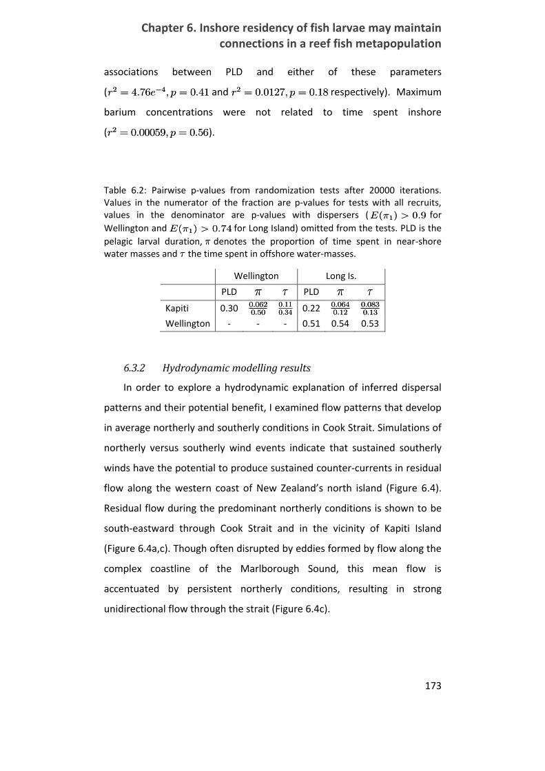
Chapter 6. Inshore residency of fish larvae may maintain connections in a reef fish metapopulation
173
associations between PLD and either of these parameters
(r2 = 4:76e¡4; p = 0:41r2 = 4:76e¡4; p = 0:41 and r2 = 0:0127; p = 0:18r2 = 0:0127; p = 0:18 respectively). Maximum
barium concentrations were not related to time spent inshore
(r2 = 0:00059; p = 0:56r2 = 0:00059; p = 0:56).
Table 6.2: Pairwise p‐values from randomization tests after 20000 iterations. Values in the numerator of the fraction are p‐values for tests with all recruits, values in the denominator are p‐values with dispersers (E(¼1) > 0:9E(¼1) > 0:9 for
Wellington and E(¼1) > 0:74E(¼1) > 0:74 for Long Island) omitted from the tests. PLD is the
pelagic larval duration, ¼¼ denotes the proportion of time spent in near-shore water masses and ¿¿ the time spent in offshore water-masses.
Wellington Long Is.
PLD ¼¼ ¿¿ PLD ¼¼ ¿¿
Kapiti 0.30 0:0620:500:0620:50
0:110:340:110:34
0.22 0:0640:120:0640:12
0:0830:130:0830:13
Wellington ‐ ‐ ‐ 0.51 0.54 0.53
6.3.2 Hydrodynamic modelling results
In order to explore a hydrodynamic explanation of inferred dispersal
patterns and their potential benefit, I examined flow patterns that develop
in average northerly and southerly conditions in Cook Strait. Simulations of
northerly versus southerly wind events indicate that sustained southerly
winds have the potential to produce sustained counter-currents in residual
flow along the western coast of New Zealand’s north island (Figure 6.4).
Residual flow during the predominant northerly conditions is shown to be
south-eastward through Cook Strait and in the vicinity of Kapiti Island
(Figure 6.4a,c). Though often disrupted by eddies formed by flow along the
complex coastline of the Marlborough Sound, this mean flow is
accentuated by persistent northerly conditions, resulting in strong
unidirectional flow through the strait (Figure 6.4c).
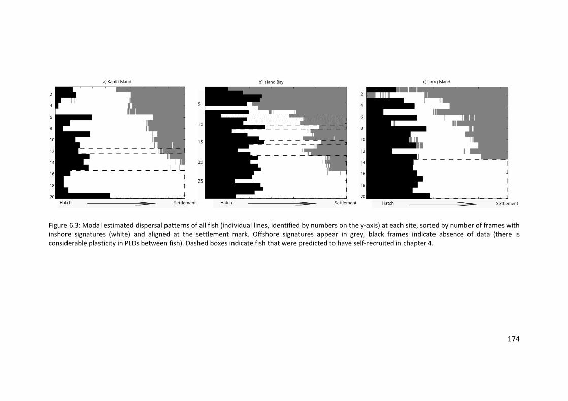
174
Figure 6.3: Modal estimated dispersal patterns of all fish (individual lines, identified by numbers on the y-axis) at each site, sorted by number of frames with inshore signatures (white) and aligned at the settlement mark. Offshore signatures appear in grey, black frames indicate absence of data (there is considerable plasticity in PLDs between fish). Dashed boxes indicate fish that were predicted to have self-recruited in chapter 4.
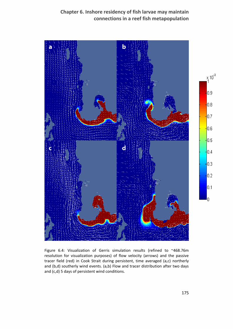
Chapter 6. Inshore residency of fish larvae may maintain connections in a reef fish metapopulation
175
Figure 6.4: Visualization of Gerris simulation results (refined to ~468.76m resolution for visualization purposes) of flow velocity (arrows) and the passive tracer field (red) in Cook Strait during persistent, time averaged (a,c) northerly and (b,d) southerly wind events. (a,b) Flow and tracer distribution after two days and (c,d) 5 days of persistent wind conditions.
6.4 Discussion
176
Persistent southerly conditions have the potential to reverse the
residual flow on the eastern border of the strait, a flow regime which gains
in breadth and velocity with on-going southerlies (Figure 6.4b,d). This flow
feature persists up the western coast of the North Island, past Kapiti Island.
Passive tracers are entrained in this residual flow along the coastline. Some
however get dispersed into the south-easterly mean flow in the strait,
often by eddies which form off the many headlands on the South eastern
border of the strait (Figure 6.4b,d).
6.4 Discussion
The stability and dynamics of marine metapopulations depend critically
on dispersal patterns within the network of local populations (Armsworth
2002, Hastings & Botsford 2006, Rozenfeld et al. 2008). These connections
may be influenced by regional hydrodynamic features (James et al. 2002,
White et al. 2010) as well as biological features of the dispersing organism
and post‐settlement processes. A number of such biological features may
influence dispersal and post settlement processes, such as larval swimming
and sensory abilities (Kingsford et al. 2002, Fisher 2005, Lecchini et al.
2005, Gerlach et al. 2007, Leis 2007), larval behaviour (Bradbury et al.
2003, Fiksen et al. 2007, Morgan & Anastasia 2008, Morgan & Fisher 2010)
as well as differential fitness induced by maternal effects and the
dispersive environment (Marshall et al. 2008, Shima & Swearer 2009a,
Marshall et al. 2010).
These, often species specific features, are the result of selective
processes which act to maintain local populations. Factors such as
fragmentation of populations may cause adaptations and selection of
dispersal strategies depending on the configuration of populations and
habitat within the dispersive ocean matrix (e.g. Baskett et al. 2007). The
interplay of local environmental conditions and their evolutionary and
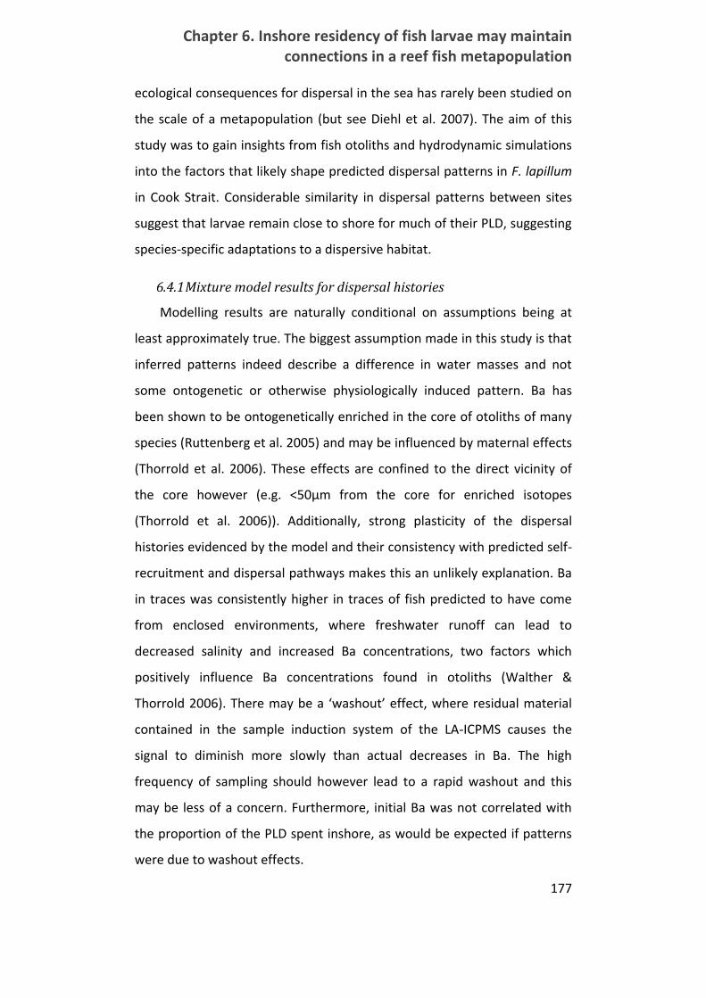
Chapter 6. Inshore residency of fish larvae may maintain connections in a reef fish metapopulation
177
ecological consequences for dispersal in the sea has rarely been studied on
the scale of a metapopulation (but see Diehl et al. 2007). The aim of this
study was to gain insights from fish otoliths and hydrodynamic simulations
into the factors that likely shape predicted dispersal patterns in F. lapillum
in Cook Strait. Considerable similarity in dispersal patterns between sites
suggest that larvae remain close to shore for much of their PLD, suggesting
species-specific adaptations to a dispersive habitat.
6.4.1 Mixture model results for dispersal histories
Modelling results are naturally conditional on assumptions being at
least approximately true. The biggest assumption made in this study is that
inferred patterns indeed describe a difference in water masses and not
some ontogenetic or otherwise physiologically induced pattern. Ba has
been shown to be ontogenetically enriched in the core of otoliths of many
species (Ruttenberg et al. 2005) and may be influenced by maternal effects
(Thorrold et al. 2006). These effects are confined to the direct vicinity of
the core however (e.g. <50μm from the core for enriched isotopes
(Thorrold et al. 2006)). Additionally, strong plasticity of the dispersal
histories evidenced by the model and their consistency with predicted self-
recruitment and dispersal pathways makes this an unlikely explanation. Ba
in traces was consistently higher in traces of fish predicted to have come
from enclosed environments, where freshwater runoff can lead to
decreased salinity and increased Ba concentrations, two factors which
positively influence Ba concentrations found in otoliths (Walther &
Thorrold 2006). There may be a ‘washout’ effect, where residual material
contained in the sample induction system of the LA-ICPMS causes the
signal to diminish more slowly than actual decreases in Ba. The high
frequency of sampling should however lead to a rapid washout and this
may be less of a concern. Furthermore, initial Ba was not correlated with
the proportion of the PLD spent inshore, as would be expected if patterns
were due to washout effects.
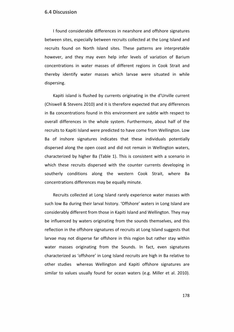
6.4 Discussion
178
I found considerable differences in nearshore and offshore signatures
between sites, especially between recruits collected at the Long Island and
recruits found on North Island sites. These patterns are interpretable
however, and they may even help infer levels of variation of Barium
concentrations in water masses of different regions in Cook Strait and
thereby identify water masses which larvae were situated in while
dispersing.
Kapiti island is flushed by currents originating in the d’Urville current
(Chiswell & Stevens 2010) and it is therefore expected that any differences
in Ba concentrations found in this environment are subtle with respect to
overall differences in the whole system. Furthermore, about half of the
recruits to Kapiti Island were predicted to have come from Wellington. Low
Ba of inshore signatures indicates that these individuals potentially
dispersed along the open coast and did not remain in Wellington waters,
characterized by higher Ba (Table 1). This is consistent with a scenario in
which these recruits dispersed with the counter currents developing in
southerly conditions along the western Cook Strait, where Ba
concentrations differences may be equally minute.
Recruits collected at Long Island rarely experience water masses with
such low Ba during their larval history. ‘Offshore’ waters in Long Island are
considerably different from those in Kapiti Island and Wellington. They may
be influenced by waters originating from the sounds themselves, and this
reflection in the offshore signatures of recruits at Long Island suggests that
larvae may not disperse far offshore in this region but rather stay within
water masses originating from the Sounds. In fact, even signatures
characterized as ‘offshore’ in Long Island recruits are high in Ba relative to
other studies whereas Wellington and Kapiti offshore signatures are
similar to values usually found for ocean waters (e.g. Miller et al. 2010).
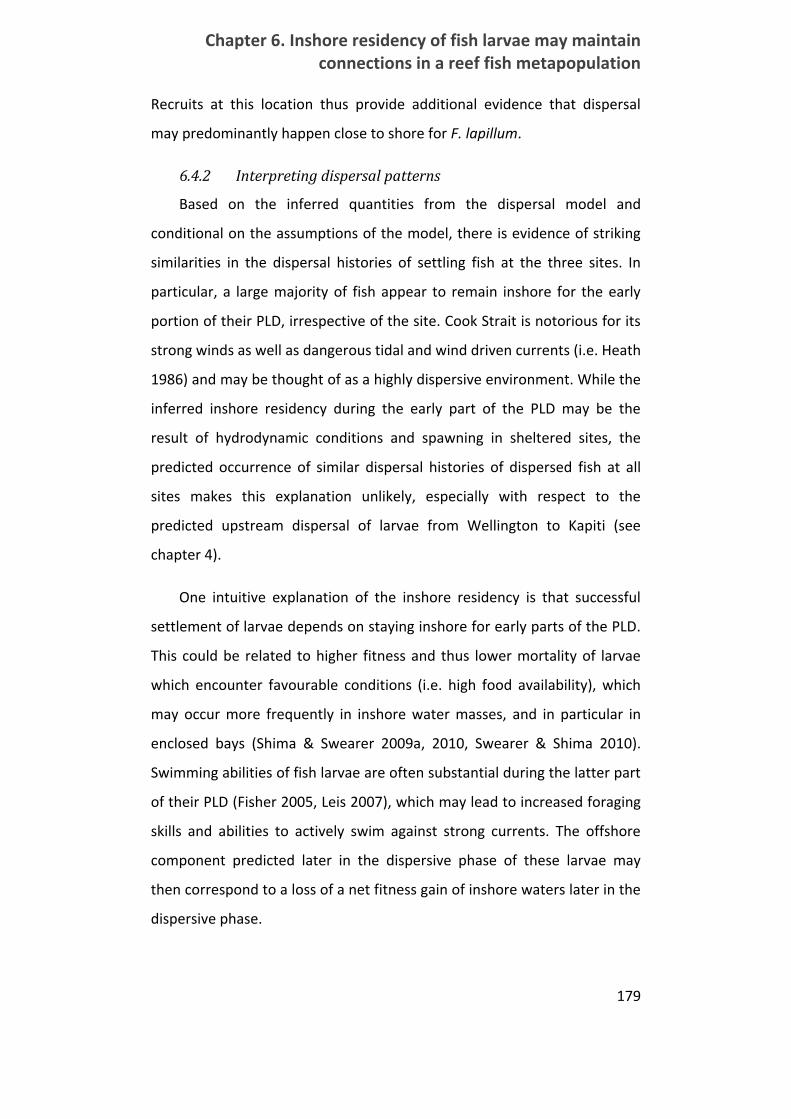
Chapter 6. Inshore residency of fish larvae may maintain connections in a reef fish metapopulation
179
Recruits at this location thus provide additional evidence that dispersal
may predominantly happen close to shore for F. lapillum.
6.4.2 Interpreting dispersal patterns
Based on the inferred quantities from the dispersal model and
conditional on the assumptions of the model, there is evidence of striking
similarities in the dispersal histories of settling fish at the three sites. In
particular, a large majority of fish appear to remain inshore for the early
portion of their PLD, irrespective of the site. Cook Strait is notorious for its
strong winds as well as dangerous tidal and wind driven currents (i.e. Heath
1986) and may be thought of as a highly dispersive environment. While the
inferred inshore residency during the early part of the PLD may be the
result of hydrodynamic conditions and spawning in sheltered sites, the
predicted occurrence of similar dispersal histories of dispersed fish at all
sites makes this explanation unlikely, especially with respect to the
predicted upstream dispersal of larvae from Wellington to Kapiti (see
chapter 4).
One intuitive explanation of the inshore residency is that successful
settlement of larvae depends on staying inshore for early parts of the PLD.
This could be related to higher fitness and thus lower mortality of larvae
which encounter favourable conditions (i.e. high food availability), which
may occur more frequently in inshore water masses, and in particular in
enclosed bays (Shima & Swearer 2009a, 2010, Swearer & Shima 2010).
Swimming abilities of fish larvae are often substantial during the latter part
of their PLD (Fisher 2005, Leis 2007), which may lead to increased foraging
skills and abilities to actively swim against strong currents. The offshore
component predicted later in the dispersive phase of these larvae may
then correspond to a loss of a net fitness gain of inshore waters later in the
dispersive phase.
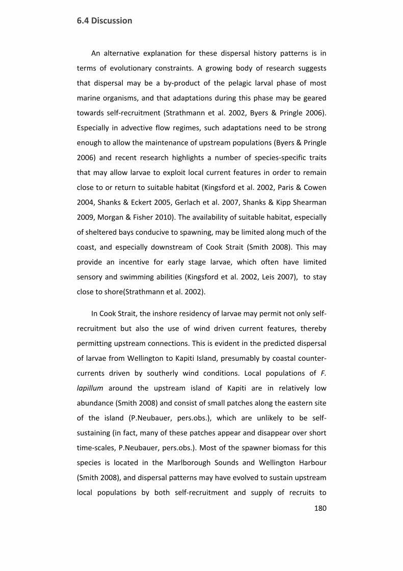
6.4 Discussion
180
An alternative explanation for these dispersal history patterns is in
terms of evolutionary constraints. A growing body of research suggests
that dispersal may be a by-product of the pelagic larval phase of most
marine organisms, and that adaptations during this phase may be geared
towards self-recruitment (Strathmann et al. 2002, Byers & Pringle 2006).
Especially in advective flow regimes, such adaptations need to be strong
enough to allow the maintenance of upstream populations (Byers & Pringle
2006) and recent research highlights a number of species-specific traits
that may allow larvae to exploit local current features in order to remain
close to or return to suitable habitat (Kingsford et al. 2002, Paris & Cowen
2004, Shanks & Eckert 2005, Gerlach et al. 2007, Shanks & Kipp Shearman
2009, Morgan & Fisher 2010). The availability of suitable habitat, especially
of sheltered bays conducive to spawning, may be limited along much of the
coast, and especially downstream of Cook Strait (Smith 2008). This may
provide an incentive for early stage larvae, which often have limited
sensory and swimming abilities (Kingsford et al. 2002, Leis 2007), to stay
close to shore(Strathmann et al. 2002).
In Cook Strait, the inshore residency of larvae may permit not only self-
recruitment but also the use of wind driven current features, thereby
permitting upstream connections. This is evident in the predicted dispersal
of larvae from Wellington to Kapiti Island, presumably by coastal counter-
currents driven by southerly wind conditions. Local populations of F.
lapillum around the upstream island of Kapiti are in relatively low
abundance (Smith 2008) and consist of small patches along the eastern site
of the island (P.Neubauer, pers.obs.), which are unlikely to be self-
sustaining (in fact, many of these patches appear and disappear over short
time-scales, P.Neubauer, pers.obs.). Most of the spawner biomass for this
species is located in the Marlborough Sounds and Wellington Harbour
(Smith 2008), and dispersal patterns may have evolved to sustain upstream
local populations by both self-recruitment and supply of recruits to
Chapter 6. Inshore residency of fish larvae may maintain connections in a reef fish metapopulation
181
upstream sinks. If the latter is a simple coincidental consequence of an
adaptation to self-recruitment, then F. lapillum populations at Kapiti may
be an ‘accidental sink’ produced by the specific current reversals in the
western Cook Strait.
6.4.3 Conclusions
Uncovering the mechanisms that underlie the structure of populations
is of importance for spatial management of marine resources and their
conservation. Larval dispersal between marine reserves and from reserves
to fished areas are two appealing features of marine reserve networks in
the context of conservation and fisheries management (Botsford et al.
2001, Roberts et al. 2001). Dispersal in such systems is likely to depend on
a range of biological, physical and evolutionary factors, and estimates of
connectivity are typically associated with large uncertainty (Halpern et al.
2006). Demonstrating which factors govern connections and self‐
recruitment patterns in a network is therefore pivotal in the development
of accurate dispersal estimates.
This study sheds some light on the potential mechanisms which allow
dispersal and maintenance of local F. lapillum populations in Cook Strait.
While the simulations employed in this chapter are abstract illustrations of
current variability under different wind regimes, empirical results and
simulation outcomes combined provide strong evidence that dispersal of
F.lapillum in Cook Strait may largely happen away from the relatively
invariable geostrophic mean currents in Cook Strait. This in turn suggests
that occasional nearshore current reversals may have a disproportionate
effect on dispersal outcomes, and could lead to upstream connectivity on
ecological timescales. While the factors affecting dispersal patterns and the
evolution of dispersal strategies are likely species specific, species with
similar life histories may be affected by similar environmental and selective
forces and may thus respond in similar ways (i.e. Shanks & Eckert 2005)

6.4 Discussion
182
and insights about representative species may help explain observations or
predict dispersal of species with similar life histories.

183
Chapter 7
7. Discussion and perspectives
The aim of this thesis was to investigate the use of new statistical and
hydrodynamic simulation methods for inference of population connectivity
of F. lapillum from otolith chemical signatures. In developing these
methods, I sought to address and improve upon a number of shortcomings
inherent in both otolith chemical approaches and the statistical methods
commonly used to analyse this geochemical data. The solutions proposed
in this thesis may be particularly useful for marine applications, where the
use of such methods often poses logistical and inferential problems.
Gaining a reliable snapshot, let alone a long term picture of inter-patch
connectivity, has been a major challenge in marine metapopulations. Even
with sophisticated tracking methods such as geochemical fingerprints or
paternity testing, one would have to track propagules from all patches to
their destination in order to gain a complete understanding of connections
in a metapopulation. Unless a species spawns and settles in very distinct
areas, this will often not be realistically possible or logistically feasible.
Tracking approaches can, however, shed light on realized connections and
the mechanism behind such connectivity (Thorrold et al. 2001, Thorrold et
al. 2002, Almany et al. 2007, Planes et al. 2009). The mere existence of
such connections, beyond their potential ecological importance, has
evolutionary implications as a genetically homogenizing force and potential
source of recruits for extinct patches. Such connections may therefore not
only drive metapopulation dynamics but also guarantee the persistence of
Discussion and perspectives
184
a metapopulation as a whole (Botsford et al. 2001, Armsworth 2002, Hill et
al. 2002, Hastings & Botsford 2006, Campbell Grant et al. 2010).
Developing new Bayesian approaches for tracking of fish larvae in the
marine environment was an essential part of my thesis, which allowed me
to make inferences about realized connections amongst local F. lapillum
populations and potential mechanisms of evidenced connectivity in Cook
Strait. Coupling tracking methods to hydrodynamic simulations lent
credibility to connections predicted from otolith chemistry, and, vise-versa,
finding such connections indicated that mean field hydrodynamics are a
valuable predictor of some connections. The simulation carried out for
chapter 4 also revealed discrepancies between predicted connectivity and
mean flows in Cook Strait, and motivated a more refined set of simulations
and a closer look at dispersal histories of F. lapillum recruits. This study, in
turn, evidenced patterns in dispersal histories across all sites that
potentially represent species-specific adaptations to the highly dispersive
ocean matrix in and around Cook Strait. Combining and contrasting
simulation and empirical estimates of connectivity can thus provide
considerable insight into patterns that drive connectivity in a
metapopulation. Building such mechanistic understanding of dispersal may
ultimately lead to a better understanding of marine metapopulation
dynamics and could thus help to better design spatial management and
conservation approaches.
The statistical methods presented in this thesis are a step towards
greater applicability of otolith chemical approaches in oceanic
environments. Specifically, the potential presence of extra baseline sources
in the sample of recruits or a mixed fisheries sample has thus far posed
problems when applying otolith chemistry in marine settings. In this
respect, the exclusion method presented in chapter 1 is likely of greater
value for exploratory purposes or for specific ecological scenarios than for
185
overall connectivity studies. The exclusion test provides an easy yet
powerful method for simple questions such as import or export of larvae
from a marine reserve. However, this test is shown to perform poorly on
larger scales, and estimates of its exclusion potential are strongly
dependent on the sampled proportion of the overall variability of chemical
signatures in a system.
Dirichlet process mixtures (DPM) are shown to perform well in
simulations and can detect extra baseline samples if these are sufficiently
different from the sampled geochemical atlas. On the opposite end of the
spectrum, the application to weakfish in chapter 3 showed that if most fish
likely came from extra baseline sources (or if sampling methods differ
between mixture and baseline, and the data is slightly ‘off’), there may be
little information about dispersal to be gained from an application of the
DPM model alone. If appropriate, the DPM classification procedure can be
considerably more informative in such situations. However, this classifier
may not always be appropriate. For species with a widespread distribution
and potential long distance dispersal, only a range-wide sampling scheme
would allow for such classification to be performed in a meaningful way.
But in such scenarios it may well be that otolith geochemistry reaches the
limits of its resolving power on scales far smaller than the distributional
range of the species. DPM based methods can thus provide a valuable tool
in many situations in which it is difficult or impossible to construct a
complete atlas. They do not, however, present a quick fix method which
does away with fundamental problems that are inherent in otolith
chemical approaches, such as low resolution or low coverage of the
chemical variability found in the dispersal range of a species by a
(relatively) small baseline sample.
Dispersal histories may be more telling about mechanisms that
underlie predicted dispersal patterns, and chapter 5 outlines a range of
Discussion and perspectives
186
possibilities to model dispersal patterns and to choose appropriate models.
While chapter six provides an arguably simplistic application of this
modelling framework, the ability to detect common dispersal patterns (or
contingents) and to quantify their similarity is a powerful tool for dispersal
studies. Shanks & Eckert (2005), for instance, hypothesized that fish with
different habitat preferences with respect to distance from shore may have
evolved to similarly exploit current variability and up/downwelling regimes
along the Californian coast. Provided these water masses are chemically
distinguishable (i.e. high Barium in upwelled waters), one could test such a
hypothesis with a representative multi-species dataset and assess whether
similarities in dispersal histories exist for species with similar niches.
A valuable extension of the present work would be to investigate the
importance of the connectivity patterns for population dynamics of F.
lapillum. Recent work by Shima & Swearer, for instance, indicates that
fitness and thus the successful recruitment of F. lapillum depends strongly
on their dispersal histories (Shima & Swearer 2009a, Shima & Swearer
2009b, Shima & Swearer 2010, Swearer & Shima 2010). Dispersers may
thus be selected against, thereby dampening the importance of dispersal
for population maintenance. Similarly, phenotype-environment
mismatches for larvae which dispersed but are not adapted to the new
environment may markedly lower the importance of such connections for
local populations (Marshall et al. 2010). Assessing the importance of
individual dispersal pathways to overall population connectivity is a
daunting task since it involves not only finding these pathways but also
following dispersed cohorts throughout their life and assessing their
reproductive output. Nevertheless such studies are possible in manageable
systems and may be increasingly manageable in other systems for which
dispersal pathways have been identified (i.e. Almany et al. 2007, Planes et
al. 2009).

187
Even if the relative importance of dispersers for population dynamics
may be relatively low, the rescue potential of these connections, however,
can be of vital importance on evolutionary time-scales (Hill et al. 2002,
Campbell Grant et al. 2010). Although dispersed recruits may be of lower
fitness and have higher mortality or lower reproductive output,
environmental changes or catastrophic events can reverse the odds over
long time scales, and these connections would then help maintain
populations. This is of considerable importance for conservation and
management of marine resources, where the desired outcome is often the
long term viability of a resource or a depleted population (Botsford et al.
2001, Fogarty & Botsford 2007).
188
Bibliography
Almany GR, Berumen ML, Thorrold SR, Planes S, Jones GP (2007) Local
replenishment of coral reef fish populations in a marine reserve.
Science 316:742-744
Anderson MJ (2001) A new method for non-parametric multivariate
analysis of variance. Austral Ecol 26:32-46
Anderson MJ, Gorley RN, Clarke KR (2008) PERMANOVA+ for
PRIMER: Guide to Software and Statistical Methods. PRIMER-E,
Plymouth, UK
Arkema KK, Abramson SC, Dewsbury BM (2006) Marine ecosystem-based
management: from characterization to implementation. Front Ecol
Environ 4:525-532
Armsworth PR (2001) Directed motion in the sea: efficient swimming by
reef fish larvae. J Theor Biol 210:81-91
Armsworth PR (2002) Recruitment limitation, population regulation, and
larval connectivity in reef fish metapopulations. Ecology 83:1092-
1104
Armsworth PR, James MK, Bode L (2001) When to press on or turn back:
dispersal strategies for reef fish larvae. Am Nat 157:434-450
Artzy-Randrup Y, Stone L (2010) Connectivity, Cycles, and Persistence
Thresholds in Metapopulation Networks. PLoS Comput Biol
6:e1000876
Ashford J, La Mesa M, Fach BA, Jones C, Everson I (2010) Testing early
life connectivity using otolith chemistry and particle-tracking
simulations. Can J Fish Aquat Sci 67:1303-1315
Avasthi A (2005) Ecosystem management - California tries to connect its
scattered marine reserves. Science 308:487-488
Barbee NC, Swearer SE (2007) Characterizing natal source population
signatures in the diadromous fish Galaxias maculatus, using
embryonic otolith chemistry. Mar Ecol Prog Ser 343:273-282
Barnett-Johnson R, Pearson TE, Ramos FC, Grimes CB, MacFarlane RB
(2008) Tracking natal origins of salmon using isotopes, otoliths, and
landscape geology. Limnol Oceanogr 53:1633-1642
Baskett ML, Weitz JS, Levin SA (2007) The evolution of dispersal in
reserve networks. Am Nat 170:59-78
Becker BJ, Levin LA, Fodrie FJ, McMillan PA (2007) Complex larval
connectivity patterns among marine invertebrate populations. Proc
Natl Acad Sci U S A 104:3267-3272
Berumen ML, Walsh HJ, Raventos N, Planes S, Jones GP, Starczak V,
Thorrold SR (2010) Otolith geochemistry does not reflect dispersal
history of clownfish larvae. Coral Reefs 29:883-891
Black KP, Moran PJ (1991) Influence of hydrodynamics on the passive
dispersal and initial recruitment of larvae of Acanthaster planci

189
(Echinodermata: Asteroidea) on the Great Barrier Reef. Mar Ecol
Prog Ser 69:55-65
Bohnsack JA (1998) Application of marine reserves to reef fisheries
management. Aust J Ecol 23:298-304
Bolker BM, Okuyama T, Bjorndal KA, Bolten AB (2007) Incorporating
multiple mixed stocks in mixed stock analysis: 'many-to-many'
analyses. Mol Ecol 16:685-695
Botsford LW (2005) Potential contributions of marine reserves to
sustainable fisheries: Recent modeling results. Bull Mar Sci 76:245-
259
Botsford LW, Castilla JC, Peterson CH (1997) The management of fisheries
and marine ecosystems. Science 277:509-515
Botsford LW, Hastings A, Gaines SD (2001) Dependence of sustainability
on the configuration of marine reserves and larval dispersal. Ecol
Lett 4:144-150
Bowman MJ, Kibblewhite AC, Murtagh RA, Chiswell SM, Sanderson BG
(1983) Circulation and mixing in greater Cook Strait, New Zealand.
Oceanol Acta 6:383-391
Bradbury IR, Campana SE, Bentzen P (2008) Estimating contemporary
early life-history dispersal in an estuarine fish: integrating molecular
and otolith elemental approaches. Mol Ecol 17:1438-1450
Bradbury IR, Snelgrove PVR, Pepin P (2003) Passive and active
behavioural contributions to the patchiness and spatial pattern during
the early life history of marine fishes. Mar Ecol Prog Ser 257:233-
245
Breitburg DL, Palmer MA, Loher T (1995) Larval distributions and the
spatial patterns of settlement of an oyster reef fish: responses to flow
and structure. Mar Ecol Prog Ser 125:45-60
Brophy D, Jeffries TE, Danilowicz BS (2004) Elevated manganese
concentrations at the cores of clupeid otoliths: possible
environmental, physiological, or structural origins. Mar Biol
144:779-786
Burkard RE, Rendl F (1984) A thermodynamically motivated simulation
procedure for combinatorial optimization problems. European
Journal of Operational Research 17:169-174
Burton RK, Koch PL (1999) Isotopic tracking of foraging and long-distance
migration in northeastern Pacific pinnipeds. Oecologia 119:578-585
Byers J, E., Pringle JM (2006) Going against the flow: retention, range
limits and invasions in advective environments. Mar Ecol Prog Ser
313:27-41
Caley MJ, Carr MH, Hixon MA, Hughes TP, Jones GP, Menge BA (1996)
Recruitment and the local dynamics of open marine populations.
Annu Rev Ecol Syst 27:477-500
Campana SE (1999) Chemistry and composition of fish otoliths: pathways,
mechanisms and applications. Mar Ecol Prog Ser 188:263-297
Campana SE (2005) Otolith science entering the 21st century. Mar Freshw
Res 56:485-495
190
Campana SE, Chouinard GA, Hanson JM, Frechet A, Brattey J (2000)
Otolith elemental fingerprints as biological tracers of fish stocks.
Fisheries Research 46:343-357
Campana SE, Thorrold SR (2001) Otoliths, increments and elements: keys
to a comprehensive understanding of fish populations? Can J Fish
Aquat Sci 58:30-38
Campana SE, Valentin A, Sevigny DM, Power D (2007) Tracking seasonal
migrations of redfish (Sebastes spp.) in and around the Gulf of St.
Lawrence using otolith elemental fingerprints. Can J Fish Aquat Sci
64:6-18
Campbell Grant EH, Nichols JD, Lowe WH, Fagan WF (2010) Use of
multiple dispersal pathways facilitates amphibian persistence in
stream networks. Proceedings of the National Academy of Sciences
107:6936-6940
Camus PA, Lima M (2002) Populations, metapopulations, and the open-
closed dilemma: the conflict between operational and natural
population concepts. Oikos 97:433-438
Cappé O, Moulines E, Rydén T (2005) Inference in hidden Markov models,
Vol. Springer, New York ; London
Casella G, Robert CP (1996) Rao-Blackwellisation of sampling schemes.
Biometrika 83:81-94
Chevenet F, Brun C, Banuls A-L, Jacq B, Christen R (2006) TreeDyn:
towards dynamic graphics and annotations for analyses of trees.
BMC Bioinformatics 7:439
Chib S (1995) Marginal Likelihood from the Gibbs Output. J Amer
Statistical Assoc 90:1313-1321
Chiswell SM, Stevens CL (2010) Lagrangian and Eulerian estimates of
circulation in the lee of Kapiti Island, New Zealand. Cont Shelf Res
30:515-532
Chittaro PM, Hogan JD, Gagnon J, Fryer BJ, Sale PF (2006) In situ
experiment of ontogenetic variability in the otolith chemistry of
Stegastes partitus. Mar Biol 149:1227-1235
Clark CW (1996) Marine reserves and the precautionary management of
fisheries. Ecol Appl 6:369-370
Clark JS (2003) Uncertainty and variability in demography and population
growth: a hierarchical approach. Ecology 84:1370-1381
Clements KD (2003) Triplefins. In: Andrew N, Francis M (eds) The Living
Reef: The Ecology of New Zealand's Rocky Reefs. Craig Potton
Publishing, Nelson, p 160-167
Clobert J, Le Galliard J-F, Cote J, Meylan S, Massot M (2009) Informed
dispersal, heterogeneity in animal dispersal syndromes and the
dynamics of spatially structured populations. Ecol Lett 12:197-209
Cornuet JM, Piry S, Luikart G, Estoup A, Solignac M (1999) New methods
employing multilocus genotypes to select or exclude populations as
origins of individuals. Genetics 153:1989-2000
Cowen R, Lwiza KMM, Sponaugle S, Paris CB, Olson DB (2000)
Connectivity of marine populations: open or closed? Science
287:857-859

191
Cowen RK, Gawarkiewic G, Pineda J, Thorrold SR, Werner FE (2007)
Population Connectivity in Marine Systems An Overview.
Oceanography 20:14-21
Cowen RK, Paris CB, Srinivasan A (2006) Scaling of connectivity in
marine populations. Science 311:522-527
Crooks KR, Sanjayan MA (2006) Connectivity conservation, Vol.
Cambridge University Press, Cambridge :
Cudney-Bueno R, Lavin MF, Marinone SG, Raimondi PT, Shaw WW
(2009) Rapid Effects of Marine Reserves via Larval Dispersal. PLoS
ONE 4
Cushing DH (1990) Plankton production and year-class strenght in fish
populations - an update of the match mismatch hypothesis. Adv Mar
Biol 26:249-293
Dahl DB (2003) An improved merge-split sampler for conjugate Dirichlet
process mixture models. Report No. #1086, University of
Wisconsin-Madison . Madison, Wisc
Dahlgren CP, Eggleston DB (2000) Ecological processes underlying
ontogenetic habitat shifts in a coral reef fish. Ecology 81:2227-2240
Dawson KJ, Belkhir K (2001) A Bayesian approach to the identification of
panmictic populations and the assignment of individuals. Genetics
Research 78:59-77
Dawson KJ, Belkhir K (2009) An agglomerative hierarchical approach to
visualization in Bayesian clustering problems. Heredity 103:32-45
Diehl JM, Toonen RJ, Botsford LW (2007) Spatial variability of recruitment
in the sand crab Emerita analoga throughout California in relation to
wind-driven currents. Marine Ecology-Progress Series 350:1-17
Doherty PJ (1981) Coral Reef Fishes: Recruitment-Limited Assemblages?
Proceedings of the Fourth International Coral Reef Symposium,
Manila 2:465-670
Dupanloup I, Schneider S, Excoffier L (2002) A simulated annealing
approach to define the genetic structure of populations. Mol Ecol
11:2571-2581
Elsdon T, Wells B, Campana S, Gillanders B, Jones C, Limburg K, Secor D,
Thorrold S, Walther B (2008) Otolith Chemistry To Describe
Movements And Life-History Parameters Of Fishes. In:
Oceanography and Marine Biology, Vol null. CRC Press, p 297-330
Elsdon TS, Gillanders BM (2003) Reconstructing migratory patterns of fish
based on environmental influences on otolith chemistry. Rev Fish
Biol Fish 13:219-235
Elsdon TS, Gillanders BM (2004) Fish otolith chemistry influenced by
exposure to multiple environmental variables. J Exp Mar Biol Ecol
313:269-284
Elsdon TS, Gillanders BM (2005) Consistency of patterns between
laboratory experiments and field collected fish in otolith chemistry:
an example and applications for salinity reconstructions. Mar Freshw
Res 56:609-617
Elsdon TS, Gillanders BM (2006) Temporal variability in strontium,
calcium, barium, and manganese in estuaries: Implications for
192
reconstructing environmental histories of fish from chemicals in
calcified structures. Estuarine Coastal Shelf Sci 66:147-156
Escobar MD, West M (1995) Bayesian Density Estimation and Inference
Using Mixtures. J Amer Statistical Assoc 90:577-588
Fablet R, Daverat F, De Pontual H (2007) Unsupervised Bayesian
reconstruction of individual life histories from otolith signatures:
case study of Sr : Ca transects of European eel (Anguilla anguilla)
otoliths. Can J Fish Aquat Sci 64:152-165
Feary DA, Clements KD (2006) Habitat use by triplefin species
(Tripterygiidae) on rocky reefs in New Zealand. J Fish Biol 69:1031-
1046
Ferguson T (1973) A Bayesian Analysis of Some Nonparametric Problems.
The Annals of Statistics 1:209-230
Feyrer F, Hobbs J, Baerwald M, Sommer T, Yin QZ, Clark K, May B,
Bennett W (2007) Otolith microchemistry provides information
complementary to microsatellite DNA for a migratory fish. Trans
Am Fish Soc 136:469-476
Fiksen O, Jorgensen C, Kristiansen T, Vikebo F, Huse G (2007) Linking
behavioural ecology and oceanography: larval behaviour determines
growth, mortality and dispersal. Marine Ecology-Progress Series
347:195-205
Fisher R (2005) Swimming speeds of larval coral reef fishes: impacts on
self-recruitment and dispersal. Marine Ecology-Progress Series
285:223-232
Fogarty MJ, Botsford LW (2007) Population Connectivity and Spatial
Management of Marine Fisheries. Oceanography 20:112-123
Fontes J, Caselle JE, Sheehy MS, Santos RS, Warner RR (2009) Natal
signatures of juvenile Coris julis in the Azores: investigating
connectivity scenarios in an oceanic archipelago. Mar Ecol Prog Ser
387:51-59
Forrester GE, Swearer SE (2002) Trace elements in otoliths indicate the use
of open-coast versus bay nursery habitats by juvenile California
halibut. Mar Ecol Prog Ser 241:201-213
Fowler AJ, Gillanders BM, Hall KC (2005) Relationship between elemental
concentration and age from otoliths of adult snapper (Pagrus auratus,
Sparidae): implications for movement and stock structure. Mar
Freshw Res 56:661-676
Gaines SD, Gaylord B, Gerber LR, Hastings A, Kinlan BP (2007)
Connecting Places The Ecological Consequences of Dispersal in the
Sea. Oceanography 20:90-99
Gaylord B, Gaines SD (2000) Temperature or transport? Range limits in
marine species mediated solely by flow. Am Nat 155:769-789
Gelman A, Carlin J, Stern H, Rubin D (2003) Bayesian Data Analysis,
Second Edition (Chapman & Hall/CRC Texts in Statistical Science),
Vol. Chapman & Hall
Gerlach G, Atema J, Kingsford MJ, Black KP, Miller-Sims V (2007)
Smelling home can prevent dispersal of reef fish larvae. Proceedings
of the National Academy of Sciences 104:858-863

193
Gilg MR, Hilbish TJ (2003) The geography of marine larval dispersal:
coupling genetics with fine-scale physical oceanography. Ecology
84:2989-2998
Gilks WR, Richardson S, Spiegelhalter DJ (1996) Markov chain Monte
Carlo in practice, Vol. Chapman & Hall, London ; New York
Gillanders BM (2002) Connectivity between juvenile and adult fish
populations: do adults remain near their recruitment estuaries? Mar
Ecol Prog Ser 240:215-223
Gillanders BM (2005) Using elemental chemistry of fish otoliths to
determine connectivity between estuarine and coastal habitats.
Estuarine Coastal Shelf Sci 64:47-57
Gillanders BM, Kingsford MJ (2000) Elemental fingerprints of otoliths of
fish may distinguish estuarine 'nursery' habitats. Mar Ecol Prog Ser
201:273-286
Gouhier TC, Guichard F, Menge BA (2010) Ecological processes can
synchronize marine population dynamics over continental scales.
Proceedings of the National Academy of Sciences 107:8281-8286
Guenette S, Lauck T, Clark C (1998) Marine reserves: from Beverton and
Holt to the present. Rev Fish Biol Fish 8:251-272
Guichard F, Bourget E, Robert J-L (2001) Scaling the influence of
topographic heterogeniety on intertidal benthic communities:
alternate trajectories mediated by hydrodynamics and shading. Mar
Ecol Prog Ser 217:27-41
Guichard F, Levin SA, Hastings A, Siegel D (2004) Toward a dynamic
metacommunity approach to marine reserve theory. Bioscience
54:1003-1011
Hale R, Swearer SE (2008) Otolith microstructural and microchemical
changes associated with settlement in the diadromous fish Galaxias
maculatus. Marine Ecology-Progress Series 354:229-234
Halpern BS, Regan HM, Possingham HP, McCarthy MA (2006)
Accounting for uncertainty in marine reserve design. Ecol Lett 9:2-
11
Hamilton SL, Regetz J, Warner RR (2008) Postsettlement survival linked to
larval life in a marine fish. Proc Natl Acad Sci U S A 105:1561-1566
Hamilton SL, Warner RR (2009) Otolith barium profiles verify the timing
of settlement in a coral reef fish. Marine Ecology-Progress Series
385:237-244
Hanski I (1999) Metapopulation Ecology, Vol. Oxford University Press
Hastie T, Tibshirani R (1996) Discriminant Analysis by Gaussian Mixtures.
Journal of the Royal Statistical Society Series B (Methodological)
58:155-176
Hastings A, Botsford LW (1999) Equivalence in yield from marine reserves
and traditional fisheries management. Science 284:1537-1538
Hastings A, Botsford LW (2006) Persistence of spatial populations depends
on returning home. Proc Natl Acad Sci U S A 103:6067-6072
Hauser L, Seamons TR, Dauer M, Naish KA, Quinn TP (2006) An
empirical verification of population assignment methods by marking
194
and parentage data: hatchery and wild steelhead (Oncorhynchus
mykiss) in Forks Creek, Washington, USA. Mol Ecol 15:3157-3173
Hawkes C (2009) Linking movement behaviour, dispersal and population
processes: is individual variation a key? J Anim Ecol 78:894-906
Heath RA (1985) A review of the physical oceanography of the seas around
New Zealand — 1982. N Z J Mar Freshwater Res 19:79-124
Heath RA (1986) In which direction is the mean flow through Cook Strait,
New Zealand - evidence of 1 to 4 week variability. N Z J Mar
Freshwater Res 20:119-137
Hedger RD, Atkinson PM, Thibault I, Dodson JJ (2008) A quantitative
approach for classifying fish otolith strontium: Calcium sequences
into environmental histories. Ecol Inform 3:207-217
Heller KA, Ghahramani Z (2005) Bayesian hierarchical clustering
Proceedings of the 22nd international conference on Machine
learning. ACM, Bonn, Germany, p 297-304
Hill MF, Hastings A, Botsford LW (2002) The effects of small dispersal
rates on extinction times in structured metapopulation models. Am
Nat 160:389-402
Hobson KA (1999) Tracing origins and migration of wildlife using stable
isotopes: a review. Oecologia 120:314-326
Huelsenbeck JP, Andolfatto P (2007) Inference of population structure
under a Dirichlet process model. Genetics 175:1787-1802
Hutchings JA (2000) Collapse and recovery of marine fishes. Nature
406:882-885
Jain S, Neal RM (2004) A split-merge Markov chain Monte Carlo
procedure for the dirichlet process mixture model. Journal of
Computational and Graphical Statistics 13:158-182
James MK, Armsworth PR, Mason LB, Bode L (2002) The structure of reef
fish metapopulations: modelling larval dispersal and retention
patterns. Proceedings of the Royal Society of London Series B-
Biological Sciences 269:2079-2086
Jax K, Jones CG, Pickett STA (1998) The self-identity of ecological units.
Oikos 82:253-264
Jones GP, Milicich MJ, Emslie MJ, Lunow C (1999) Self-recruitment in a
coral reef fish population. Nature 402:802-804
Jordan MI (2004) Graphical models. Statistical Science 19:140-155
Kass RE, Raftery AE (1995) Bayes Factors. J Amer Statistical Assoc
90:773-795
Kelly L, Stefan L (2007) New Zealand's Quota Management System: A
History of the First 20 Years, Motu Economic and Public Policy
Research
Kendall BE, Bjoernstad ON, Bascompte J, Keitt TH, Fagan WF (2000)
Dispersal, Environmental Correlation, and Spatial Synchrony in
Population Dynamics. The American Naturalist 155:628-636
Kingsford MJ, Leis JM, Shanks A, Lindeman KC, Morgan SG, Pineda J
(2002) Sensory environments, larval abilities, and local self-
recruitment. Bull Mar Sci 70:309-340
195
Koehl MAR, Strother JA, Reidenbach MA, Koseff JR, Hadfield MG (2007)
Individual-based model of larval transport to coral reefs in turbulent,
wave-driven flow: behavioral responses to dissolved settlement
inducer. Mar Ecol Prog Ser 335:1-18
Kohn Y (2007) Pelagic larval duration in New Zealand triplefin fishes.
University of Auckland
Koljonen ML, Pella JJ, Masuda M (2005) Classical individual assignments
versus mixture modeling to estimate stock proportions in Atlantic
salmon (Salmo salar) catches from DNA microsatellite data. Can J
Fish Aquat Sci 62:2143-2158
Kritzer JP, Sale PF (2004) Metapopulation ecology in the sea: from Levins'
model to marine ecology and fisheries science. Fish Fish 5:131-140
Largier JL (2003) Considerations in estimating larval dispersal distances
from oceanographic data. Ecol Appl 13:S71-S89
Lecchini D (2005) Spatial and behavioural patterns of reef habitat
settlement by fish larvae. Marine Ecology-Progress Series 301:247-
252
Lecchini D, Shima J, Banaigs B, Galzin R (2005) Larval sensory abilities
and mechanisms of habitat selection of a coral reef fish during
settlement. Oecologia 143:326-334
Leis J, Stobutzki I (1999) Swimming performance of late pelagic larvae of
coral-reef fishes: in situ and laboratory-based measurments.
Proceedings from the 5th Indo-Pacific Fish Conference, Noumea
1999:1-9
Leis JM (2007) Behaviour as input for modelling dispersal of fish larvae:
behaviour, biogeography, hydrodynamics, ontogeny, physiology,
and phylogeny meet hydrography. Mar Ecol Prog Ser 347:185-193
Leis JM, Carson-Ewart BM (2003) Orientation of pelagic larvae of coral-
reef fishes in the ocean. Mar Ecol Prog Ser 252:239-253
Levin LA (2006) Recent progress in understanding larval dispersal: new
directions and digressions. Integr Comp Biol 46:282-297
Levins R (1969) Some demographic and genetic consequences of
environmental heterogeniety for biological control. Bull Entomol
Soc Am 15:237-240
Lockwood DR, Hastings A (2002) The effects of dispersal patterns on
marine reserves: does the tail wag the dog? Theor Popul Biol
61:297-309
Lunn DJ, Thomas A, Best N, Spiegelhalter D (2000) WinBUGS - A
Bayesian modelling framework: Concepts, structure, and
extensibility. Statistics and Computing 10:325-337
Mace AJ, Morgan SG (2006) Larval accumulation in the lee of a small
headland: implications for the design of marine reserves. Marine
Ecology-Progress Series 318:19-29
Manel S, Gaggiotti OE, Waples RS (2005) Assignment methods: matching
biological questions techniques with appropriate. Trends Ecol Evol
20:136-142
Marine_Zooplankton_Colloquium_2 (2001) Future marine zooplankton
research--a perspective. Mar Ecol Prog Ser 222:297-308

196
Marshall DJ, Allen RM, Crean AJ (2008) The ecological and evolutionary
importance of maternal effects in the sea. In: Oceanography and
Marine Biology: an Annual Review, Vol 46, Vol 46. Crc Press-
Taylor & Francis Group, Boca Raton, p 203-250
Marshall DJ, Monro K, Bode M, Keough MJ, Swearer S (2010) Phenotype-
environment mismatches reduce connectivity in the sea. Ecol Lett
13:128-140
Mercier L, Darnaude A, Bruguier O, Vasconcelos R, Costa M, Cabral H,
Lara M, Jones D, Mouillot D (in press) Selecting statistical models
and variable combinations for optimal classification using otolith
microchemistry. Ecol Appl
Millar RB (1987) Maximum likelihood estiamtion of mixed stock fishery
composition. Can J Fish Aquat Sci 44:583-590
Miller JA (2007a) Scales of variation in otolith elemental chemistry of
juvenile staghorn sculpin (Leptocottus armatus) in three Pacific
Northwest estuaries. Mar Biol 151:483-494
Miller JA, Gray A, Merz J (2010) Quantifying the contribution of juvenile
migratory phenotypes in a population of Chinook salmon
Oncorhynchus tshawytscha. Mar Ecol Prog Ser 408:227-240
Miller TJ (2007b) Contribution of individual-based coupled physical-
biological models to understanding recruitment in marine fish
populations. Mar Ecol Prog Ser 347:127-138
Mitarai S, Siegel DA, Winters KB (2008) A numerical study of stochastic
larval settlement in the California Current system. J Mar Syst
69:295-309
Morel FMM, Price NM (2003) The biogeochemical cycles of trace metals in
the oceans. Science 300:944-947
Morgan SG, Anastasia JR (2008) Behavioral tradeoff in estuarine larvae
favors seaward migration over minimizing visibility to predators.
Proceedings of the National Academy of Sciences 105:222-227
Morgan SG, Fisher JL (2010) Larval behavior regulates nearshore retention
and offshore migration in an upwelling shadow and along the open
coast. Mar Ecol Prog Ser 404:109-126
Msadek R (2005) Hydrodynamic tidal model of Cook Strait, National
Institute of Water and Atmospheric Research, Wellington, NZ
Munch SB, Clarke LM (2008) A Bayesian approach to identifying mixtures
from otolith chemistry data. Can J Fish Aquat Sci 65:2742-2751
Nahas EL, Jackson G, Pattiaratchi CB, Ivey GN (2003) Hydrodynamic
modelling of snapper Pagrus auratus egg and larval dispersal in
Shark Bay, Western Australia: reproductive isolation at a fine spatial
scale. Marine Ecology-Progress Series 265:213-226
Neal R (1992) Bayesian Mixture Modeling. In: Smith CR, Erickson GJ,
Neudorfer PO (eds) Maximum Entropy and Bayesian Methods:
Proceedings of the 11th International Workshop on Maximum
Entropy and Bayesian Methods of Statistical Analysis, Seattle, 1991.
Kluwer Academic Publishers, Dordrecht, p 197-211
197
Neal R (2000) Markov Chain Sampling Methods for Dirichlet Process
Mixture Models. Journal of Computational and Graphical Statistics
9:249-265
Neubauer P, Hadfield M, Delaux S, Popinet S, Shima JS (in prep)
Validation of an adaptive grid ocean model for simulation of larval
dispersal in Cook Strait, New Zealand.
Neubauer P, Shima JS, Swearer SE (2010) Scale-dependent variability in
natal otolith chemistry: implications and solutions for studies of
population connectivity. Mar Ecol Prog Ser 415:263-274
Ohlssen DI, Sharples LD, Spiegelhalter DJ (2007) Flexible random-effects
models using Bayesian semi-parametric models: applications to
institutional comparisons. Stat Med 26:2088-2112
Palumbi SR (1994) Genetic divergence, reproductive isolation, and marine
speciation. Annu Rev Ecol Syst 25:547-572
Palumbi SR (2003) Population genetics, demographic connectivity, and the
design of marine reserves. Ecol Appl 13:S146-S158
Paris CB, Cowen RK (2004) Direct evidence of a biophysical retention
mechanism for coral reef fish larvae. Limnol Oceanogr 49:1964-
1979
Patterson TA, Basson M, Bravington MV, Gunn JS (2009) Classifying
movement behaviour in relation to environmental conditions using
hidden Markov models. J Anim Ecol 78:1113-1123
Patterson TA, Thomas L, Wilcox C, Ovaskainen O, Matthiopoulos J (2008)
State-space models of individual animal movement. Trends Ecol
Evol 23:87-94
Pauly D, Christensen V, Guenette S, Pitcher TJ, Sumaila UR, Walters CJ,
Watson R, Zeller D (2002) Towards sustainability in world fisheries.
Nature 418:689-695
Peck MA, Daewel U (2007) Physiologically based limits to food
consumption, and individual-based modeling of foraging and growth
of larval fishes. Mar Ecol Prog Ser 347:171-183
Pella J, Masuda M (2001) Bayesian methods for analysis of stock mixtures
from genetic characters. Fish Bull 99:151-167
Pella J, Masuda M (2006) The Gibbs and split-merge sampler for population
mixture analysis from genetic data with incomplete baselines. Can J
Fish Aquat Sci 63:576-596
Pikitch EK, Santora C, Babcock EA, Bakun A, Bonfil R, Conover DO,
Dayton P, Doukakis P, Fluharty D, Heneman B, Houde ED, Link J,
Livingston PA, Mangel M, McAllister MK, Pope J, Sainsbury KJ
(2004) ECOLOGY: Ecosystem-Based Fishery Management. Science
305:346-347
Planes S, Jones GP, Thorrold SR (2009) Larval dispersal connects fish
populations in a network of marine protected areas. Proc Natl Acad
Sci U S A 106:5693-5697
Popinet S (2003) Gerris: a tree-based adaptive solver for the incompressible
Euler equations in complex geometries. Journal of Computational
Physics 190:572-600

198
Popinet S, Rickard G (2007) A tree-based solver for adaptive ocean
modelling. Ocean Model Online 16:224-249
Roberts CM (1997) Connectivity and management of Caribbean coral reefs.
Science 278:1454-1457
Roberts CM, Bohnsack JA, Gell F, Hawkins JP, Goodridge R (2001) Effects
of marine reserves on adjacent fisheries. Science 294:1920-1923
Royer T, Fromentin J-M, Gaspar P (2005) A state-space model to derive
bluefin tuna movement and habitat from archival tags. Oikos
109:473-484
Rozenfeld AF, Arnaud-Haond S, Hernández-GarcÃa E, EguÃluz VcM,
Serrão EA, Duarte CM (2008) Network analysis identifies weak
and strong links in a metapopulation system. Proceedings of the
National Academy of Sciences 105:18824-18829
Rubenstein DR, Chamberlain CP, Holmes RT, Ayres MP, Waldbauer JR,
Graves GR, Tuross NC (2002) Linking Breeding and Wintering
Ranges of a Migratory Songbird Using Stable Isotopes. Science
295:1062-1065
Rubenstein DR, Hobson KA (2004) From birds to butterflies: animal
movement patterns and stable isotopes. Trends Ecol Evol 19:256-
263
Ruttenberg BI, Hamilton SL, Hickford MJH, Paradis GL, Sheehy MS,
Standish JD, Ben-Tzvi O, Warner RR (2005) Elevated levels of trace
elements in cores of otoliths and their potential for use as natural
tags. Mar Ecol Prog Ser 297:273-281
Ruttenberg BI, Hamilton SL, Warner RR (2008) Spatial and temporal
variation in the natal otolith chemistry of a Hawaiian reef fish:
prospects for measuring population connectivity. Can J Fish Aquat
Sci 65:1181-1192
Ruttenberg BI, Warner RR (2006) Spatial variation in the chemical
composition of natal otoliths from a reef fish in the Galapagos
Islands. Mar Ecol Prog Ser 328:225-236
Ruzzante DE, Mariani S, Bekkevold D, Andre C, Mosegaard H, Clausen
LAW, Dahlgren TG, Hutchinson WF, Hatfield EMC, Torstensen E,
Brigham J, Simmonds EJ, Laikre L, Larsson LC, Stet RJM, Ryman
N, Carvalho GR (2006) Biocomplexity in a highly migratory pelagic
marine fish, Atlantic herring. Proceedings of the Royal Society B-
Biological Sciences 273:1459-1464
Sale P (1998) Appropriate spatial scales for studies of reef-fish ecology.
Aust J Ecol 23:202-208
Sale PF, Cowen RK, Danilowicz BS, Jones GP, Kritzer JP, Lindeman KC,
Planes S, Polunin NVC, Russ GR, Sadovy YJ, Steneck RS (2005)
Critical science gaps impede use of no-take fishery reserves. Trends
Ecol Evol 20:74-80
Sandin SA, Regetz J, Hamilton SL (2005) Testing larval fish dispersal
hypotheses using maximum likelihood analysis of otolith chemistry
data. Mar Freshw Res 56:725-734
Schaefer JA (2006) Towards maturation of the population concept. Oikos
112:236-240

199
Schick RS, Loarie SR, Colchero F, Best BD, Boustany A, Conde DA,
Halpin PN, Joppa LN, McClellan CM, Clark JS (2008)
Understanding movement data and movement processes: current and
emerging directions. Ecol Lett 11:1338-1350
Schnute JT, Richards LJ (2001) Use and abuse of fishery models. Can J Fish
Aquat Sci 58:10-17
Scott SL (2002) Bayesian methods for hidden Markov models: Recursive
computing in the 21st century. J Amer Statistical Assoc 97
Secor D, Piccoli P (1996) Age- and sex-dependent migrations of striped
bass in the Hudson River as determined by chemical microanalysis
of otoliths. Estuar Coasts 19:778-793
Secor DH (1999) Specifying divergent migrations in the concept of stock:
the contingent hypothesis. Fisheries Research 43:13-34
Shanks AL (2009) Pelagic Larval Duration and Dispersal Distance
Revisited. Biol Bull 216:373-385
Shanks AL, Eckert GL (2005) Population persistence of California Current
fishes and benthic crustaceans: A marine drift paradox. Ecol Monogr
75:505-524
Shanks AL, Grantham BA, Carr MH (2003) Propagule dispersal distance
and the size and spacing of marine reserves. Ecol Appl 13:S159-
S169
Shanks AL, Kipp Shearman R (2009) Paradigm lost? Cross-shelf
distributions of intertidal invertebrate larvae are unaffected by
upwelling or downwelling. Mar Ecol Prog Ser 385:189-204
Shima JS, Swearer SE (2009a) Larval quality is shaped by matrix effects:
implications for connectivity in a marine metapopulation. Ecology
90:1255-1267
Shima JS, Swearer SE (2009b) Spatially variable larval histories may shape
recruitment rates of a temperate reef fish. Marine Ecology-Progress
Series 394:223-229
Shima JS, Swearer SE (2010) The legacy of dispersal: larval experience
shapes persistence later in the life of a reef fish. J Anim Ecol
79:1308-1314
Siegel DA, Kinlan BP, Gaylord B, Gaines SD (2003) Lagrangian
descriptions of marine larval dispersion. Mar Ecol Prog Ser 260:83-
96
Siegel DA, Mitarai S, Costello CJ, Gaines SD, Kendall BE, Warner RR,
Winters KB (2008) The stochastic nature of larval connectivity
among nearshore marine populations. Proc Natl Acad Sci U S A
105:8974-8979
Smedbol RK, Wroblewski JS (2002) Metapopulation theory and northern
cod population structure: interdependency of subpopulations in
recovery of a groundfish population. Fisheries Research 55:161-174
Smith ANH (2008) Predicting the distribution and relative abundance of
fishes on shallow subtidal reefs around New Zealand, NIWA,
Wellington
200
Smith SJ, Campana SE (2010) Integrated stock mixture analysis for
continous and categorical data, with application to genetic-otolith
combinations. Can J Fish Aquat Sci 67:1533-1548
Smouse PE, Spielman RS, Park MH (1982) Multiple-locus allocation of
individuals to groups as a function of the genetic variation within
and differences among human populations. Am Nat 119:445-463
Standish JD, Sheehy M, Warner RR (2008) Use of otolith natal elemental
signatures as natural tags to evaluate connectivity among open-coast
fish populations. Mar Ecol Prog Ser 356:259-268
Stobutzki IC (2001) Marine reserves and the complexity of larval dispersal.
Rev Fish Biol Fish 10:515-518
Strathmann RR, Hughes TP, Kuris AM, Lindeman KC, Morgan SG,
Pandolfi JM, Warner RR (2002) Evolution of local recruitment and
its consequences for marine populations. Bull Mar Sci 70:377-396
Swearer S, Caselle J, Lea D, Warner R (1999) Larval retention and
recruitment in an island population of a coral reef fish. Nature
402:799-802
Swearer SE, Shima JS (2010) Regional variation in larval retention and
dispersal drives recruitment patterns in a temperate reef fish. Mar
Ecol Prog Ser 417:229-236
Swearer SE, Shima JS, Helberg ME, Thorrold SR, Jones GP, Robertson DR,
Morgan SG, Selkoe KA, Ruiz GM, Warner RR (2002) Evidence of
self-recruitment in demersal marine populations. Bull Mar Sci
70:251-271
Szép T, Møller AP, Vallner J, Kovács B, Norman D (2003) Use of trace
elements in feathers of sand martin Riparia riparia for identifying
moulting areas. J Avian Biol 34:307-320
Taylor MS, Hellberg ME (2003) Genetic evidence for local retention of
pelagic larvae in a Caribbean reef fish. Science 299:107-109
Team RDC (2007) R: A language and environment for statistical
computing. R Foundation for Statistical Computing. R Foundation
for Statistical Computing, Vienna, Austria
Thorrold S, Jones C, Swart P, Targett T (1998) Acurate classification of
juvenile weakfish Cynoscion regalis to estuarine nursery areas based
on chemical signatures in otoliths. Mar Ecol Prog Ser 173:253-265
Thorrold SR, Jones GP, Helberg ME, Burton RS, Swearer SE, Neigel JE,
Morgan SG, Warner RR (2002) Quantifying larval retention and
connectivity in marine populations with artificial and natural
markers. Bull Mar Sci 70:291-308
Thorrold SR, Jones GP, Planes S, Hare JA, Dt (2006) Transgenerational
marking of embryonic otoliths in marine fishes using barium stable
isotopes. Can J Fish Aquat Sci 63:1193-1197
Thorrold SR, Latkoczy C, Swart PK, Jones CM (2001) Natal homing in a
marine fish metapopulation. Science 291:297-299
Treml EA, Halpin PN, Urban DL, Pratson LF (2008) Modeling population
connectivity by ocean currents, a graph-theoretic approach for
marine conservation. Landsc Ecol 23:19-36
201
Walther BD, Thorrold SR (2006) Water, not food, contributes the majority
of strontium and barium deposited in the otoliths of a marine fish.
Mar Ecol Prog Ser 311:125-130
Waples RS, Gaggiotti O (2006) What is a population? An empirical
evaluation of some genetic methods for identifying the number of
gene pools and their degree of connectivity. Mol Ecol 15:1419-1439
Warner RR, Swearer SE, Caselle JE, Sheehy M, Paradis G (2005) Natal
trace-elemental signatures in the otoliths of an open-coast fish.
Limnol Oceanogr 50:1529-1542
Wellenreuther M, Barrett PT, Clements KD (2007) Ecological
diversification in habitat use by subtidal triplefin fishes
(Tripterygiidae). Mar Ecol Prog Ser 330:235-246
Wellenreuther M, Clements KD (2007) Reproductive isolation in temperate
reef fishes. Mar Biol
White C, Kendall BE (2007) A reassessment of equivalence in yield from
marine reserves and traditional fisheries managament. Oikos
116:2039-2043
White JW, Botsford LW, Hastings A, Largier JL (2010) Population
persistence in marine reserve networks: incorporating spatial
heterogeneities in larval dispersal. Mar Ecol Prog Ser 398:49-67
White JW, Ruttenberg BI (2006) Discriminant function analysis in marine
ecology: some oversights and their solutions. Mar Ecol Prog Ser
329:301-305
White JW, Standish JD, Thorrold SR, Warner RR (2008) Makov Chain
Monte Carlo Methods for assigning larvae to natal sites using natural
geochemical tags. Ecol Appl 18:1901-1913
Zacherl DC (2005) Spatial and temporal variation in statolith and
protoconch trace elements as natural tags to track larval dispersal.
Marine Ecology-Progress Series 290:145-163
Zimmer RK, Fingerut JT, Zimmer CA (2009) Dispersal pathways, seed
rains, and the dynamics of larval behavior. Ecology 90:1933-1947
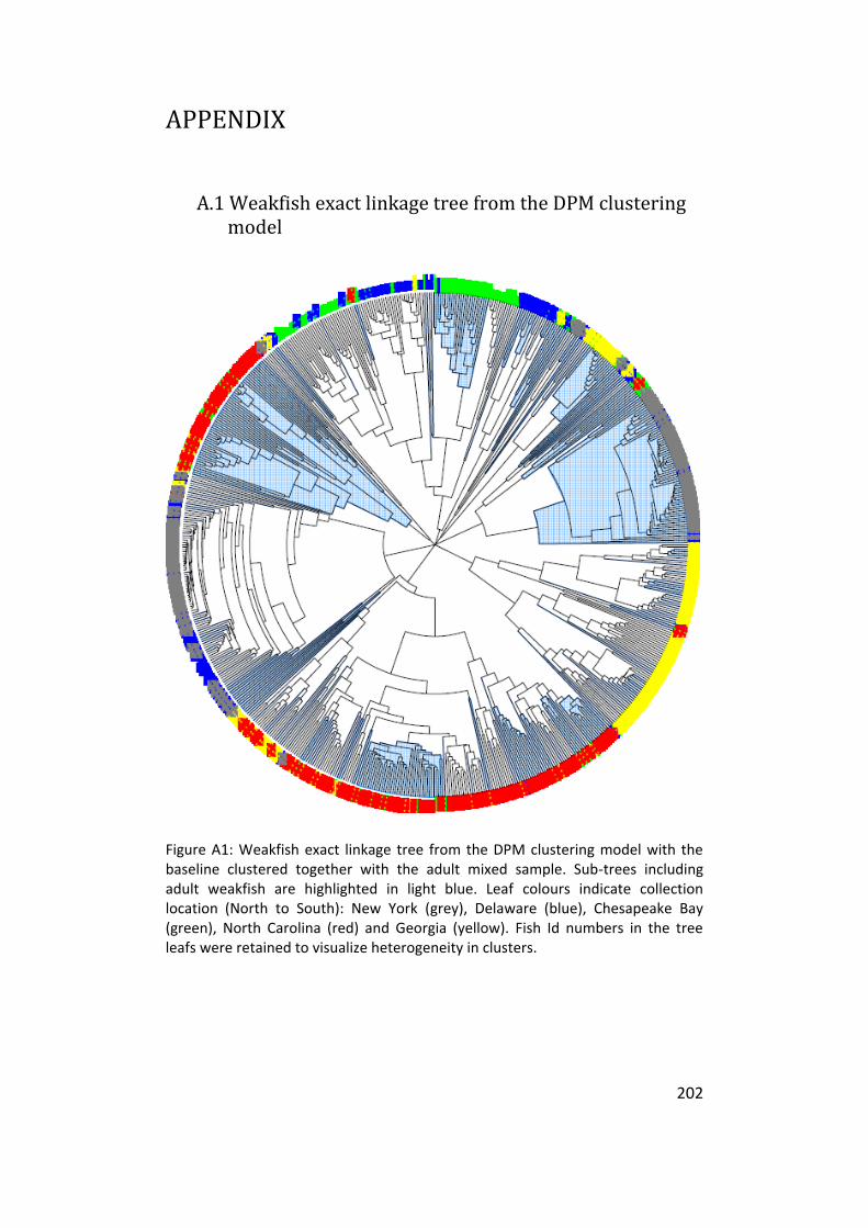
202
APPENDIX
A.1 Weakfish exact linkage tree from the DPM clustering model
Figure A1: Weakfish exact linkage tree from the DPM clustering model with the baseline clustered together with the adult mixed sample. Sub-trees including adult weakfish are highlighted in light blue. Leaf colours indicate collection location (North to South): New York (grey), Delaware (blue), Chesapeake Bay (green), North Carolina (red) and Georgia (yellow). Fish Id numbers in the tree leafs were retained to visualize heterogeneity in clusters.

203
A.2 Gibbs sampling in the mixture models
The relevant conditional posteriors are given here for a two component
random effects mixture model discussed in chapter 5, from which those of
easier models can be readily obtained by omitting the random effects. I
then give the procedure to sample the state sequence from the HMM in
appendix A.3. Some posteriors (those involving T) require slight
modification if transects have an unequal number of observations.
1. Start by drawing »i;t»i;t at iteration s=1 of the Gibbs sampler,
conditional on all other parameters as
»i;tj¼i; µ » Bernoulli(zi;t)
zi;ts =¼iN(yi;tj¹+ ºi;¾
2º)
¼iN(yi;tj¹+ ºi;¾2º) + (1¡ ¼i)N(yi;tj¹;¾2
¹)
»i;tj¼i; µ » Bernoulli(zi;t)
zi;ts =¼iN(yi;tj¹+ ºi;¾
2º)
¼iN(yi;tj¹+ ºi;¾2º) + (1¡ ¼i)N(yi;tj¹;¾2
¹)
2. I then update the mixture proportions (for more than one class this
becomes a Dirichlet distribution.
¼ij³ » Beta
Ã
1 +
TX
t=1
»i;t; 1 + (T ¡
TX
t=1
»i;t)
!
¼ij³ » Beta
Ã
1 +
TX
t=1
»i;t; 1 + (T ¡
TX
t=1
»i;t)
!
3. Draw ¹¹ as
¹jµ; ³ » N
ÃPN
i=1
PT
t=1 yi;t ¡ »i;t´i
NT;¾2¹
NT
!
¹jµ; ³ » N
ÃPN
i=1
PT
t=1 yi;t ¡ »i;t´i
NT;¾2¹
NT
!
4. The random effects ´́ are updated as
´ijµ; »i » N
Ã1&2®+
PT
t=1
»i;t
¾2º(yi;t ¡ ¹)
1&2+
PT
t=11¾2º
;1
1&2+
PT
t=11¾2º
!
´ijµ; »i » N
Ã1&2®+
PT
t=1
»i;t
¾2º(yi;t ¡ ¹)
1&2+
PT
t=11¾2º
;1
1&2+
PT
t=11¾2º
!
5. Next I update the mean of the random effects
®jµ » N
ÃPN
i=1 ´i
N;&2
N
!
®jµ » N
ÃPN
i=1 ´i
N;&2
N
!
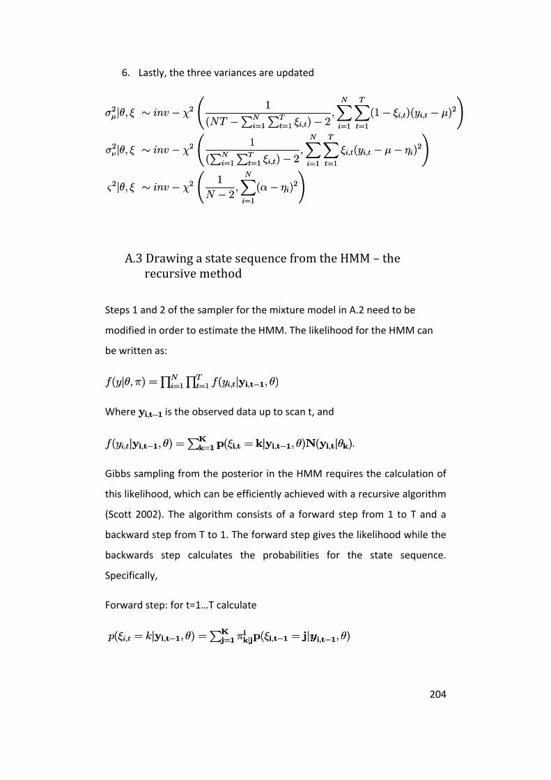
204
6. Lastly, the three variances are updated
¾2¹jµ; » » inv ¡ Â2
Ã1
(NT ¡PN
i=1
PT
t=1 »i;t)¡ 2;
NX
i=1
TX
t=1
(1¡ »i;t)(yi;t ¡ ¹)2
!
¾2ºjµ; » » inv ¡ Â2
Ã1
(PN
i=1
PT
t=1 »i;t)¡ 2;
NX
i=1
TX
t=1
»i;t(yi;t ¡ ¹¡ ´i)2
!
&2jµ; » » inv ¡ Â2
Ã1
N ¡ 2;
NX
i=1
(®¡ ´i)2
!
¾2¹jµ; » » inv ¡ Â2
Ã1
(NT ¡PN
i=1
PT
t=1 »i;t)¡ 2;
NX
i=1
TX
t=1
(1¡ »i;t)(yi;t ¡ ¹)2
!
¾2ºjµ; » » inv ¡ Â2
Ã1
(PN
i=1
PT
t=1 »i;t)¡ 2;
NX
i=1
TX
t=1
»i;t(yi;t ¡ ¹¡ ´i)2
!
&2jµ; » » inv ¡ Â2
Ã1
N ¡ 2;
NX
i=1
(®¡ ´i)2
!
A.3 Drawing a state sequence from the HMM – the recursive method
Steps 1 and 2 of the sampler for the mixture model in A.2 need to be
modified in order to estimate the HMM. The likelihood for the HMM can
be written as:
f(yjµ;¼) =QN
i=1
QT
t=1 f(yi;tjyi;t¡1;µ)f(yjµ;¼) =QN
i=1
QT
t=1 f(yi;tjyi;t¡1;µ)
Where yi;t¡1yi;t¡1 is the observed data up to scan t, and
f(yi;tjyi;t¡1;µ) =PK
k=1p(»i;t = kjyi;t¡1;µ)N(yi;tjµk)f(yi;tjyi;t¡1;µ) =PK
k=1p(»i;t = kjyi;t¡1;µ)N(yi;tjµk).
Gibbs sampling from the posterior in the HMM requires the calculation of
this likelihood, which can be efficiently achieved with a recursive algorithm
(Scott 2002). The algorithm consists of a forward step from 1 to T and a
backward step from T to 1. The forward step gives the likelihood while the
backwards step calculates the probabilities for the state sequence.
Specifically,
Forward step: for t=1…T calculate
p(»i;t = kjyi;t¡1;µ) =PK
j=1¼ikjjp(»i;t¡1 = jjyi;t¡1; µ)p(»i;t = kjyi;t¡1;µ) =
PK
j=1¼ikjjp(»i;t¡1 = jjyi;t¡1; µ)
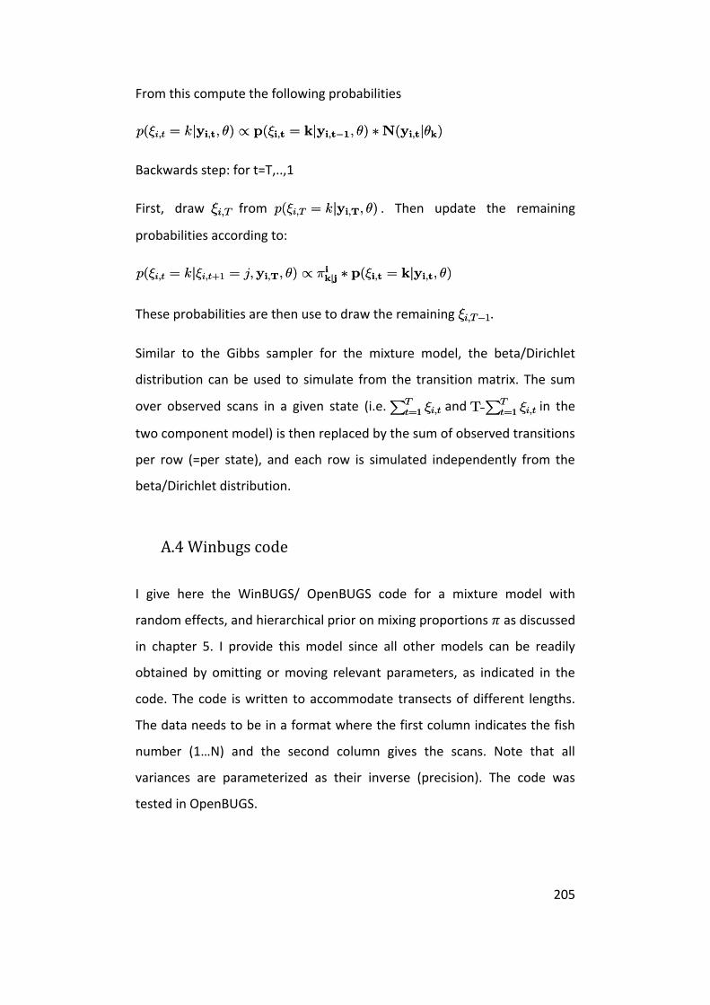
205
From this compute the following probabilities
p(»i;t = kjyi;t; µ) / p(»i;t = kjyi;t¡1; µ) ¤N(yi;tjµk)p(»i;t = kjyi;t; µ) / p(»i;t = kjyi;t¡1; µ) ¤N(yi;tjµk)
Backwards step: for t=T,..,1
First, draw »i;T»i;T from p(»i;T = kjyi;T; µ)p(»i;T = kjyi;T; µ) . Then update the remaining
probabilities according to:
p(»i;t = kj»i;t+1 = j;yi;T; µ) / ¼ikjj ¤ p(»i;t = kjyi;t; µ)p(»i;t = kj»i;t+1 = j;yi;T; µ) / ¼ikjj ¤ p(»i;t = kjyi;t; µ)
These probabilities are then use to draw the remaining »i;T¡1»i;T¡1.
Similar to the Gibbs sampler for the mixture model, the beta/Dirichlet
distribution can be used to simulate from the transition matrix. The sum
over observed scans in a given state (i.e. PT
t=1 »i;tPT
t=1 »i;t and T-PT
t=1 »i;tT-PT
t=1 »i;t in the
two component model) is then replaced by the sum of observed transitions
per row (=per state), and each row is simulated independently from the
beta/Dirichlet distribution.
A.4 Winbugs code
I give here the WinBUGS/ OpenBUGS code for a mixture model with
random effects, and hierarchical prior on mixing proportions as discussed
in chapter 5. I provide this model since all other models can be readily
obtained by omitting or moving relevant parameters, as indicated in the
code. The code is written to accommodate transects of different lengths.
The data needs to be in a format where the first column indicates the fish
number (1…N) and the second column gives the scans. Note that all
variances are parameterized as their inverse (precision). The code was
tested in OpenBUGS.

206
model{ for( j in 1 : N ) {
# mixing proportions are drawn from a Dirichlet with common prior gamma, omitting gamma leads to a non-hierarchical model. Moving props outside the for-loop gives a model with a single mixing proportion for all individuals. props[j ,1:2 ] ~ ddirich(gamma[]) # mixing proportions # random effects for mean 2, moving this outside of the for loop gives a model with two normal components
mu2[j] ~ dnorm(nu, tau) #random effects }
# TOT is N*T, or the total number of scans if these are different between individuals
for( i in 1 : TOT ) {
# Z assigns fish i to water-mass k=1,2, y[i,1] gives the fish id of scan i
Z[i] ~ dcat(props[y[i,1], ])
mu[i] <- mu1 + (2-Z[ i]) * mu2[y[i,1]] sigs[i] <- sig[Z[ i]] y[i , 2] ~ dnorm(mu[i], sigs[ i])
# The following line is used for posterior predictive checks in OpenBUGS only – leave commented out for WinBUGS
# postmu[ i] <-replicate.post(y[i , 2] ) } # common prior for mixing proportions, omit for non-hierarchical model in pi gamma[1] ~ dgamma(0.001, 0.001) gamma[2] ~ dgamma(0.001, 0.001)
# vague priors for the mean for water-mass 1 mu1 ~ dnorm(0.001, 0.0001)
#priors for individual water-mass variances sig[1] ~ dgamma(0.001, 0.001) sig[2] ~ dgamma(0.001, 0.001) # vague priors for the random effect mean for water-mass 2 nu ~ dnorm(0.001,0.001)
# random effects variance tau ~ dgamma(0.001,0.001)