Development and Application of Agglomerated

Multigrid Methods for Complex Geometries

Hiroaki Nishikawa∗, Boris Diskin†

National Institute of Aerospace, Hampton, VA 23666

and

James L. Thomas‡

NASA Langley Research Center, Hampton VA 23681

We report progress in the development of agglomerated multigrid techniques for fully un-structured grids in three dimensions, building upon two previous studies focused on efficientlysolving a model diffusion equation. We demonstrate a robust fully-coarsened agglomeratedmultigrid technique for 3D complex geometries, incorporating the following key developments:consistent and stable coarse-grid discretizations, a hierarchical agglomeration scheme, andline-agglomeration/relaxation using prismatic-cell discretizations in the highly-stretched gridregions. A significant speed-up in computer time is demonstrated for a model diffusion prob-lem, the Euler equations, and the Reynolds-averaged Navier-Stokes equations for 3D realisticcomplex geometries.

I. Introduction

Multigrid techniques [1] are used to accelerate convergence of current Reynolds-Averaged Navier-Stokes(RANS) solvers for both steady and unsteady flow solutions, particularly for structured-grid applications.Mavriplis et al. [2, 3, 4, 5] pioneered agglomerated multigrid methods for large-scale unstructured-grid applica-tions. During the present development, a serious convergence degradation in some of the state-of-the-art multi-grid algorithms was observed on highly-refined grids. To investigate and overcome the difficulty, we criticallystudied agglomerated multigrid techniques [6, 7] for two- and three-dimensional isotropic and highly-stretchedgrids and developed techniques to achieve grid-independent convergence for a model equation representing lam-inar diffusion in the incompressible limit. It was found in Ref. [6] that it is essential for grid-independentconvergence to use consistent coarse-grid discretizations. In the later Ref. [7], it was found that the use of pris-matic cells and line-agglomeration/relaxation is essential for grid-independent convergence on fully-coarsenedhighly-stretched grids. In this paper, we extend and demonstrate these techniques for practical problems:inviscid and viscous flows over complex geometries.

The paper is organized as follows. Finite-volume discretizations employed for target grids are described.Details of the hierarchical agglomeration scheme are described. Elements of the multigrid algorithm are thendescribed, including discretizations on coarse grids. Multigrid results for complex geometries are shown for amodel diffusion equation, the Euler equations, and the RANS equations. The final section contains conclusionsand recommendations for future work.

∗Senior Research Scientist (hiro@nianet.org), National Institute of Aerospace, 100 Exploration Way, Hampton, VA 23666 USA.†Associate Fellow (bdiskin@nianet.org), National Institute of Aerospace, 100 Exploration Way, Hampton, VA 23666 USA.;

Visiting Associate Professor, Mechanical and Aerospace Engineering Department, University of Virginia, Charlottesville, SeniorMember AIAA

‡Senior Research Scientist (James.L.Thomas@nasa.gov), Computational AeroSciences Branch, Mail Stop 128, Fellow AIAA.

1 of 15

American Institute of Aeronautics and Astronautics

https://ntrs.nasa.gov/search.jsp?R=20100025598 2018-07-30T12:21:59+00:00Z

4

2

1

3

0

Figure 1. Illustration of a node-centered median-dual control volume(shaded). Dual faces connect edge midpoints with primal cell centroids.Numbers 0-4 denote grid nodes.

II. Discretization

The discretization method is a finite-volume discretization (FVD) centered at nodes. It is based on theintegral form of governing equations of interest:∮

Γ

(F · n) dΓ =

∫∫Ω

s dΩ, (1)

where F is a flux tensor, s is a source term, Ω is a control volume with boundary Γ, and n is the outwardunit normal vector. For the model diffusion (Laplace) equation, the boundary conditions are taken as Dirich-let, i.e., specified from a known exact solution over the computational boundary. Tests are performed for aconstant manufactured solution, U(x, y, z) = 10.0, with a randomly perturbed initial solution. For inviscidflow problems, the governing equations are the Euler equations. Boundary conditions are a slip-wall conditionand inflow/outflow conditions on open boundaries. For viscous flow problems, the governing equations are theRANS equations with the Spalart-Allmaras one-equation model [8]. Boundary conditions are non-slip condi-tion on walls and inflow/outflow conditions on open boundaries. The source term, s, is zero except for theturbulence-model equation (see Ref. [8]).

The general FVD approach requires partitioning the domain into a set of non-overlapping control volumesand numerically implementing Equation (1) over each control volume. Node-centered schemes define solutionvalues at the mesh nodes. In 3D, the primal cells are tetrahedra, prisms, hexahedra, or pyramids. The median-dual partition [9, 10] used to generate control volumes is illustrated in Figure 1 for 2D. These non-overlappingcontrol volumes cover the entire computational domain and compose a mesh that is dual to the primal mesh.

The main target discretization of interest for the model diffusion equation and the viscous terms of the RANSequations is obtained by the Green-Gauss scheme [11, 12], which is the most widely-used viscous discretizationfor node-centered schemes and is equivalent to a Galerkin finite-element discretization for pure tetrahedral grids.For mixed-element cells, edge-based contributions are used to increase the h-ellipticity of the operator [11, 12].The inviscid terms are discretized by a standard edge-based method with unweighted least-squares gradientreconstruction and Roe’s approximate Riemann solver [13]. Limiters are not used for the problems consideredin this paper. The convection terms of the turbulence equation are discretized with first-order accuracy.

III. Agglomeration Scheme

As described in the previous papers [6,7], the grids are agglomerated within a topology-preserving framework,in which hierarchies are assigned based on connections to the computational boundaries. Corners are identifiedas grid points with three or more boundary-condition-type closures (or three or more boundary slope disconti-nuities). Ridges are identified as grid points with two boundary-condition-type closures (or two boundary slopediscontinuities). Valleys are identified as grid points with a single boundary-condition-type closure. Interiorsare identified as grid points without any boundary condition. The agglomerations proceed hierarchically fromseeds within the topologies — first corners, then ridges, then valleys, and finally interiors. Rules are enforced

2 of 15

American Institute of Aeronautics and Astronautics

Hierarchy of Agglomeration Hierarchy of Added Volume Agglomeration Admissibility

corner any disallowed

ridge interior disallowed

ridge valley disallowed

ridge ridge conditional

valley interior disallowed

valley valley conditional

interior interior allowed

Table 1. Admissible agglomerations.

Figure 2. Trailing-edge area of a 3D wing agglomeratedby the hierarchical scheme. Primal grid is shown by thinlines; agglomerated grid is shown by thick lines.

Figure 3. Typical implicit line-agglomeration showinga curved solid body surface on the left and a symme-try plane on the right. The projection of the line-agglomerations can be seen on the symmetry plane.

to maintain the boundary condition types of the finer grid within the agglomerated grid. Candidate volumesto be agglomerated are vetted against the hierarchy of the currently agglomerated volumes. In this work, weuse the rules summarized in Table 1. In order to enable a valid non-degenerate stencil for linear prolongationand least-squares gradients near boundaries [7], the rules reflect less agglomerations near boundaries than inthe interior. Corners are never agglomerated, ridges are agglomerated only with ridges, and valleys are agglom-erated only with valleys. A typical boundary agglomeration generated by the above rules is shown in Figure 2.The conditional entries denote that further inspection of the connectivity of the topology must be consideredbefore agglomeration is allowed. For example, a ridge can be agglomerated into an existing ridge agglomerationif the two boundary conditions associated with each ridge are the same. For valleys or interiors, all availableneighbors are collected and then agglomerated one by one in the order of larger number of edge-connections toa current agglomeration until the maximum threshold of agglomerated nodes (4 for valleys; 8 for interiors) isreached. The prolongation operator P1 is modified to prolong only from hierarchies equal or above the hierarchyof the prolonged point. Hierarchies on each agglomerated grid are inherited from the finer grid.

For the results reported in this paper, we employ agglomeration scheme II described in previous papers [6,7].It has been modified to deal with viscous meshes using implicit-line agglomeration. It performs the agglomerationin the following sequence:

1. Agglomerate viscous boundaries (bottom of implicit lines).

2. Agglomerate prismatic layers through the implicit lines (implicit-line agglomeration).

3. Agglomerate the rest of the boundaries.

3 of 15

American Institute of Aeronautics and Astronautics

4. Agglomerate the interior.

The second step is a line-agglomeration step where volumes are agglomerated along implicit lines starting fromthe volume directly above the boundary volume. Specifically, we first agglomerate volumes corresponding tothe second and third entries in the implicit-line lists associated with each of the fine-grid volumes contained ina boundary agglomerate. The line agglomeration continues to the end of the shortest line among the lines asso-ciated with the boundary agglomerate. This line-agglomeration process preserves the boundary agglomerates.Figure 3 illustrates typical implicit line-agglomerattion near a curved solid body. The implicit line-agglomerationpreserves the line structure of the fine grid on coarse grids, so that line-relaxations can be performed on all gridsto address the grid anisotropy. If no implicit lines are defined, typical for inviscid grids, the first two steps areskipped.

In each boundary agglomeration (steps 1 and 3), agglomeration begins with corners, creates a front listdefined by collecting volumes adjacent to the agglomerated corners, and proceeds to agglomerate volumes in thelist (while updating the list as agglomeration proceeds) in the order of ridges and valleys. During the process,a volume is selected from among those in the same hierarchy that has the least number of non-agglomeratedneighbors, thereby reducing the occurrences of agglomerations with small numbers of volumes. A heap data-structure is utilized to efficiently select such a volume. The agglomeration continues until the front list becomesempty. Finally, for both valleys and interiors, agglomerations containing only a few volumes (typically one) arecombined with other agglomerations.

Figures 4 and 5 show primal grids and agglomerations for the F6 wing-body combination and the DPW-W2[14] grids. These grids are viscous grids; the primal grid has prismatic viscous layers around the body and thewing. Coarsening ratios are indicated by rk (k = 1, 2, 3, 4) in the parenthesis. Line agglomeration was appliedin these regions. Figures 6, 7, and 8 show primal grids and agglomerations for a wing-body combination, awing-flap combination, and a 3D wing with a blunt trailing edge — all are pure-tetrahedral inviscid grids.

IV. Multigrid

Elements of the multigrid algorithm are presented in this section. In this study, we do not explore variousalgorithmic options, relying on the methods that proved effective from the previous studies.

IV.A. Multigrid V-Cycle

The multigrid method is based on the full-approximation scheme (FAS) [1, 15] where a coarse-grid problem issolved/relaxed for the solution approximation. A correction, computed as the difference between the restrictedfine-grid solution and the coarse-grid solution, is prolonged to the finer grid to update the fine-grid solution.The two-grid FAS is applied recursively through multiple coarse grids to define a V-cycle. A V-cycle, denotedas V (ν1, ν2), uses ν1 relaxations performed at each grid before proceeding to the coarser grid and ν2 relaxationsafter coarse-grid correction. On the coarsest grid, relaxations are performed to bring two orders of magnituderesidual reduction or until the maximum number of relaxations, 10, is reached.

IV.B. Inter-Grid Operators

The control volumes of each agglomerated grid are found by summing control volumes of a finer grid. Anoperator that performs the summation is given by a conservative agglomeration operator, R0, which acts onfine-grid control volumes and maps them onto the corresponding coarse-grid control-volumes. Any agglomeratedgrid can be defined, therefore, in terms of R0 as

Ωc = R0Ωf , (2)

where superscripts c and f denote entities on coarser and finer grids, respectively. On the agglomerated grids,the control volumes become geometrically more complex than their primal counterparts and the details of thecontrol-volume boundaries are not retained. The directed area of a coarse-grid face separating two agglomeratedcontrol volumes, if required, is found by lumping the directed areas of the corresponding finer-grid faces and isassigned to the virtual edge connecting the centers of the agglomerated control volumes.

Residuals on the fine grid, Rf , corresponding to the integral equation (1) are restricted to the coarse gridby the conservative agglomeration operator, R0, as

Rc = R0Rf , (3)

4 of 15

American Institute of Aeronautics and Astronautics

Inviscid Viscous

Primal grid Second-order edge-based reconstruction Green-Gauss

Coarse grids First-order edge-based reconstruction Face-Tangent Avg-LSQ

Table 2. Summary of discretizations.

where Rc denotes the fine-grid residual restricted to the coarse grid.The fine-grid solution approximation, Uf , is restricted as

U c0 =

R0(UfΩf )

Ωc, (4)

where U c0 denotes the fine-grid solution approximation restricted to the coarse grid. The restricted approximation

is then used to define the forcing term to the coarse-grid problem as well as to compute the correction, (δU)c:

(δU)c = U c − U c0 , (5)

where U c is the coarse-grid solution approximation obtained directly from the coarse-grid problem.The correction to the finer grid is prolonged typically through the prolongation operator, P1, that is exact

for linear functions, as(δU)f = P1(δU)c. (6)

The operator P1 is constructed locally using linear interpolation from a tetrahedra defined on the coarse grid.The geometrical shape is anchored at the coarser-grid location of the agglomerate that contains the given finercontrol volume. Other nearby points are found by the adjacency graph. An enclosing simplex is sought thatavoids prolongation with non-convex weights and, in situations where multiple geometrical shapes are found,the first one encountered is used. Where no enclosing simplex is found, the simplex with minimal non-convexweights is used.

IV.C. Coarse-Grid Discretizations

For the model equation and the viscous term in the RANS equations, two classes of coarse-grid discretizationswere previously studied [6, 7]: the Average-Least-Squares (Avg-LSQ) and the edge-terms-only (ETO) schemes.The Avg-LSQ scheme is a consistent discretization that uses the average of the dual-volume LSQ gradients todetermine a gradient at the face, which is augmented with the edge-based directional contribution to determinethe gradient used in the flux. There are two variants of the Avg-LSQ scheme. One uses the average-least-squares gradients in the direction normal to the edge (edge-normal gradient construction). The other uses theaverage-least-squares gradients along the face (face-tangent gradient construction).

The ETO discretizations are obtained from the Avg-LSQ schemes by taking the limit of zero Avg-LSQgradients. The ETO schemes are often cited as a thin-layer discretization in the literature [2, 3, 4]; they arepositive schemes but are not consistent (i.e., the discrete solutions do not converge to the exact continuoussolution with consistent grid refinement) unless the grid is orthogonal [13, 16]. As shown in the previouspapers [6, 7], ETO schemes lead to deterioration of the multigrid convergence for refined grids, and thereforeare not considered in this paper. For practical applications, the face-tangent Avg-LSQ scheme was found to bemore robust than the edge-normal Avg-LSQ scheme. It provides superior diagonal dominance in the resultingdiscretization [6, 7]. In this study, therefore, we employ the face-tangent Avg-LSQ scheme as a coarse-griddiscretization for the model equation and the viscous term. For excessively-skewed grids (over 90), whichcan arise on agglomerated grids, the scheme exhibits unstable behavior. For such cases, we simply ignorecontributions associated with edges with an excessive skewness angle. The Galerkin coarse-grid operator [1],which was considered in a previous study, is not considered here since the method was found to be grid-dependentand slowed down the multigrid convergence for refined grids [6]. For inviscid discretization, we employ a first-order edge-based discretization on coarse grids. Table 2 shows a summary of discretizations used.

5 of 15

American Institute of Aeronautics and Astronautics

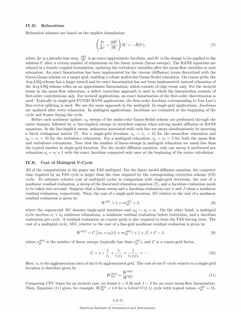
IV.D. Relaxations

Relaxation schemes are based on the implicit formulation:(Ω

∆τ+

∂R∗

∂U

)δU = −R(U), (7)

where ∆τ is a pseudo-time step, ∂R∗

∂U is an exact/approximate Jacobian, and δU is the change to be applied to thesolution U after a certain number of relaxations on the linear system (linear-sweeps). The RANS equations arerelaxed in a loosely-coupled formulation, updating the turbulence variables after the mean-flow variables at eachrelaxation. An exact linearization has been implemented for the viscous (diffusion) terms discretized with theGreen-Gauss scheme on a target grid, enabling a robust multicolor Gauss-Seidel relaxation. On coarse grids, theAvg-LSQ scheme has a larger stencil and its exact linearization has not been implemented; instead relaxation ofthe Avg-LSQ scheme relies on an approximate linearization, which consists of edge terms only. For the inviscidterms in the mean-flow relaxation, a defect correction approach is used in which the linearization consists offirst-order contributions only. For inviscid applications, an exact linearization of the first-order discretization isused. Typically in single-grid FUN3D RANS applications, the first-order Jacobian corresponding to Van Leer’sflux-vector splitting is used. We use the same approach in the multigrid. In single-grid applications, Jacobiansare updated after every relaxation. In multigrid applications, Jacobians are evaluated at the beginning of thecycle and frozen during the cycle.

Before each nonlinear update, νp sweeps of the multi-color Gauss-Seidel scheme are performed through theentire domain, followed by νl line-implicit sweeps in stretched regions when solving model diffusion or RANSequations. In the line-implicit sweep, unknowns associated with each line are swept simultaneously by invertinga block tridiagonal matrix [7]. For a single-grid iteration, νp = νl = 15 for the mean-flow relaxation andνp = νl = 10 for the turbulence relaxation. For a multigrid relaxation, νp = νl = 5 for both the mean flowand turbulence relaxations. Note that the number of linear-sweeps in multigrid relaxation are much less thanthe typical number in single-grid iteration. For the model diffusion equation, only one sweep is performed perrelaxation νp = νl = 1 with the exact Jacobian computed only once at the beginning of the entire calculation.

IV.E. Cost of Multigrid V-Cycle

All of the computations in the paper use FAS multigrid. For the linear model diffusion equation, the computertime required by an FAS cycle is larger than the time required by the corresponding correction scheme (CS)cycle. To estimate relative cost of multigrid cycles in comparison with single-grid iterations, the cost of anonlinear residual evaluation, a sweep of the linearized relaxation equation (7), and a Jacobian evaluation needsto be taken into account. Suppose that a linear sweep and a Jacobian evaluation cost σ and J times a nonlinearresidual evaluation, respectively. Then, the cost of a single-grid iteration, SG relative to the cost of a nonlinearresidual evaluation is given by

WSG = 1 + σνSGpl + J, (8)

where the superscript SG denotes single-grid iterations and νpl = νp + νl. On the other hand, a multigridcycle involves ν1 + ν2 nonlinear relaxations, a nonlinear residual evaluation before restriction, and a Jacobianevaluation per cycle. A residual evaluation on coarser grids is also required to form the FAS forcing term. Thecost of a multigrid cycle, MG, relative to the cost of a fine-grid nonlinear residual evaluation is given by

WMG = C[(ν1 + ν2)(1 + σνMG

pl ) + 1 + J]+ C − 1, (9)

where νMGpl is the number of linear sweeps (typically less than νSG

pl ), and C is a coarse-grid factor,

C = 1 +1

r1+

1

r1r2+

1

r1r2r3+ · · · . (10)

Here, rk is the agglomeration ratio of the k-th agglomerated grid. The cost of one V -cycle relative to a single-griditeration is therefore given by

WMGSG =

WMG

WSG. (11)

Comparing CPU times for an inviscid case, we found σ = 0.16 and J = 2 for an exact mean-flow linearization.Then, Equation (11) gives, for example, WMG

SG = 1.8 for a 5-level V (2, 1) cycle with typical values, νSGpl = 15,

6 of 15

American Institute of Aeronautics and Astronautics

νMGpl = 5 and the coarsening ratio of 8. Hence, a typical multigrid V (2, 1) cycle costs 1.8 single-grid iterations.As will be shown later, the above estimate is also accurate for RANS calculations.

For the model diffusion equation, the same formula applies as it is implemented in the same FAS framework.A major difference, however, lies in the Jacobian evaluation. The Jacobian is constant for the linear problem;thus it is computed only once and never updated. Therefore, the cost of the Jacobian evaluation can be ignored.For example, assuming typical values, νSG

pl = 1, νMGpl = 1 and the coarsening ratio of 8, we obtain WMG

SG = 8.0from Equation (11) for a 5-level V (3, 3) cycle.

V. Results for Complex Geometries

All calculations presented in this paper were performed with a single processor. Parallelization of themultigrid algorithm is currently underway.

V.A. Model Diffusion Equation

The multigrid method was applied on grids generated for two practical geometries: the F6 wing-body and theDPW-W2 wing-alone cases [14]. Both grids are tetrahedral, but prisms are used in a highly-stretched viscouslayer near the solid boundary. Pyramidal cells are also present around the transitional region. For these cases,a 5-level V (3, 3) multigrid cycle is applied and compared with single-grid iterations. The CFL number is set toinfinity. For the F6 wing-body grid (1,121,301 nodes), the grids and convergence results are shown in Figure 4.The speed-up factor is nearly 44 in CPU time. A similar result was obtained for the DPW-W2 grid ( 1,893,661nodes) as shown in Figure 5. The speed-up factor is nearly 24 in this case. The cost of one V -cycle computedaccording to Equation (11) with actual coarsening ratios is shown for each case in the first column of Table 4.It shows that one V-cycle costs nearly 8 single-grid relaxations. The second column is an expected speed-upfactor based on the number of single-grid iterations (NSG), the number of multigrid cycles (NMG), and thefactor WMG

SG :

NSG

NMGWMGSG

. (12)

The third column is the actual speed-up factor computed as a ratio of the total single-grid CPU time to thetotal multigrid CPU time. The table shows that the expected speed-up is 50 percent larger than the actualspeed-up so some refinement of the relative work breakdown is needed.

V.B. Inviscid Flows

The multigrid method was applied to three inviscid cases: low-speed subsonic flows over a wing-body configu-ration, a wing-flap configuration, and a NACA15 wing with a blunt trailing edge. Table 3 shows a summaryof grid sizes and parameters. Nramp denotes the number of first iterations/cycles over which the CFL numberis ramped from 10 to 200 for single-grid/multigrid calculations. The multigrid V (2, 1) cycle was employed forthese cases.

Grid Size (nodes) Inflow Mach number Angle of Attack Nramp

Wing-Body 1,012,189 0.3 0 10

Wing-Flap 1,184,650 0.3 2 10

NACA15 Wing 2,039,914 0.3 2 100

Table 3. Summary of grid sizes and parameters for the inviscid cases.

Figure 6 shows the grids and convergence results for the wing-body configuration case. As Figure 6(f)shows, the multigrid converges (to machine zero) 5 times faster in CPU time than the single-grid iterations.The convergence results for the wing-flap configuration is given in Figure 7(f). It shows that the multigridconverges (to machine zero) nearly 2 times faster in CPU time than the single-grid iterations. For the NACA15wing case, the solution does not fully converge in either single-grid or multigrid computations apparently dueto an unsteady behavior near the blunt trailing edge. However, as shown in Figure 7(f), the multigrid drivesthe residual more rapidly down to the level of 10−9 than the single-grid iteration.

7 of 15

American Institute of Aeronautics and Astronautics

Grid Flow Model V-cycleCost of V-cycle Expected Speed-up Actual Speed-up

(WMGSG ) (Equation (12)) (Using actual CPU time)

F6WB Diffusion V (3, 3) 8.3 62.7 43.5

DPW-W2 Diffusion V (3, 3) 8.3 35.1 23.8

Wing-Body Inviscid V (2, 1) 1.8 5.2 5.2

Wing-Flap Inviscid V (2, 1) 1.8 2.0 1.9

NACA15 Wing Inviscid V (2, 1) 1.8 2.9 2.8

F6WB RANS V (2, 1) 1.8 4.8 5.0

Table 4. Cost of V-cycle relative to a single-grid iteration and speed-up factor.

In all three cases, the ratio of the number of multigrid cycles to the number of single-grid iterations is abouttwice the speed-up factor in terms of the CPU time. It implies that the cost of one multigrid V (2, 1) cycleis almost equivalent to the cost of two single-grid iterations. These results are in good agreement with theestimates in Section IV.E. The cost of one V-cycle computed according to Equation (11) is shown for each casein the first column of Table 4. The cost of one V -cycle is 1.8 of the single-grid iteration cost for all cases. Theentries in the second and third columns agree well with each other.

V.C. Turbulent Flows (RANS)

We applied the multigrid algorithm to a RANS simulation on the F6 wing-body grid shown in Figure 4. Theinflow Mach number is 0.3, the angle of attack is 1 degree, and the Reynolds number is 2.5 million. For this case,a prolongation operator that is exact for a constant function is used. The P1 prolongation operator encountereda difficulty on a boundary for this particular configuration, and it is currently under investigation. The CFLnumber is not ramped in this case, but set to 200 for the mean-flow equations and 30 for the turbulence equation.

Convergence results are shown in Figure 9. As can be seen, the multigrid achieved four orders of reductionin the residual 5 times faster in CPU time than the single-grid iteration. For this case, neither the multigrid norsingle-grid method fully converges seemingly due to a separation near the wing-body junction. Four orders ofmagnitude reduction is just about how far a single-grid is run in practice for this particular configuration. Thecomparison of the number of cycles with the number of single-grid relaxations in the figure imply, again, thatthe CPU time for one multigrid V (2, 1) cycle is approximately equivalent to the CPU time for two single-griditerations. As shown in Table 4, one multigrid V-cycle actually costs 1.8 single-grid iterations.

VI. Concluding Remarks

An agglomerated multigrid algorithm has been applied to inviscid and viscous flows over complex geometries.A robust fully-coarsened hierarchical agglomeration scheme was described for highly-stretched viscous grids,incorporating consistent viscous discretization on coarse grids. Results for practical simulations show thatimpressive speed-ups are achieved for realistic flows over complex geometries.

Parallelization of the developed multigrid algorithm is currently underway to expand the applicability ofthe developed technique to larger-scale computations and to demonstrate grid-independent convergence of thedeveloped multigrid algorithm.

Acknowledgments

All results presented were computed within the FUN3D suite of codes at NASA Langley Research Center(http://fun3d.larc.nasa.gov/). This work was supported by the NASA Fundamental Aeronautics Programthrough NASA Research Announcement Contract NNL07AA23C.

References

1Trottenberg, U., Oosterlee, C. W., and Schuller, A., Multigrid , Academic Press, 2001.2Mavriplis, D. J., “Multigrid Techniques for Unstructured Meshes,” VKI Lecture Series VKI-LS 1995-02, Von Karman

Institute for Fluid Dynamics, Rhode-Saint-Genese, Belgium, 1995.

8 of 15

American Institute of Aeronautics and Astronautics

3Mavriplis, D. J., “Unstructured Grid Techniques,” Annual Review of Fluid Mechanics, Vol. 29, 1997, pp. 473–514.4Mavriplis, D. J. and Pirzadeh, S., “Large-Scale Parallel Unstructured Mesh Computations for 3D High-Lift Analysis,” Journal

of Aircraft , Vol. 36, No. 6, 1999, pp. 987–998.5Mavriplis, D. J., “An Assessment of Linear versus Non-Linear Multigrid Methods for Unstructured Mesh Solvers,” Journal

of Computational Physics, Vol. 275, 2002, pp. 302–325.6Nishikawa, H., Diskin, B., and Thomas, J. L., “Critical Study of Agglomerated Multigrid Methods for Diffusion,” AIAA

Journal , Vol. 48, No. 4, 2010, pp. 839–847.7Thomas, J. L., Diskin, B., and Nishikawa, H., “A Critical Study of Agglomerated Multigrid Methods for Diffusion on

Highly-Stretched Grids,” Computers and Fluids, 2010, to appear.8Spalart, P. R. and Allmaras, S. R., “A One-Equation Turbulence Model for Aerodynamic Flows,” AIAA paper 92-0439, 1992.9Barth, T. J., “Numerical Aspects of Computing Viscous High Reynolds Number Flows on Unstructured Meshes,” AIAA

Paper 91-0721, 1991.10Haselbacher, A. C., A Grid-Transparent Numerical Method for Compressible Viscous Flow on Mixed Unstructured Meshes,

Ph.D. thesis, Loughborough Universit, 1999.11Anderson, W. K. and Bonhaus, D. L., “An implicit upwind algorithm for computing turbulent flows on unstructured grids,”

Computers and Fluids, Vol. 23, 1994, pp. 1–21.12Diskin, B., Thomas, J. L., Nielsen, E. J., Nishikawa, H., and White, J. A., “Comparison of Node-Centered and Cell-Centered

Unstructured Finite-Volume Discretizations. Part I: Viscous Fluxes,” 47th AIAA Aerospace Sciences Meeting, AIAA Paper 2009-597, January 2009 (AIAA Journal, in press).

13Diskin, B. and Thomas, J. L., “Accuracy Analysis for Mixed-Element Finite-Volume Discretization Schemes,” NIA ReportNo. 2007-08 , 2007.

14“The DPW-II Workshop for the geometry,” http://aaac.larc.nasa.gov/tsab/cfdlarc/aiaa-dpw/Workshop2/workshop2.

html.15Briggs, W. L., Henson, V. E., and McCormick, S. F., A Multigrid Tutorial , SIAM, 2nd ed., 2000.16Thomas, J. L., Diskin, B., and Rumsey, C. L., “Towards Verification of Unstructured Grid Methods,” AIAA Journal , Vol. 46,

No. 12, December 2008, pp. 3070–3079.

9 of 15

American Institute of Aeronautics and Astronautics

(a) Level 1: primal grid. (b) Level 2: coarse grid (r1 = 6.5).

(c) Level 3: coarse grid (r2 = 6.2). (d) Level 4: coarse grid (r3 = 5.5).

(e) Level 5: coarse grid (r4 = 4.6).

0 5 10 15 20 25 30−14

−12

−10

−8

−6

−4

−2

0

2

4

CPU Time (hour)

Log

10 (

Res

idua

l )

Multigrid V(3,3): 36 cycles, 0.7 hoursSingle Grid: 18707 relaxations, 29.7 hours

(f) Convergence history: residual versus CPU time.

Figure 4. Grids and convergence of the model diffusion equation for the F6 wing-body combination.

10 of 15

American Institute of Aeronautics and Astronautics

(a) Level 1: primal grid. (b) Level 2: coarse grid (r1 = 6.3).

(c) Level 3: coarse grid (r2 = 5.8). (d) Level 4: coarse grid (r3 = 5.3).

(e) Level 5: coarse grid (r4 = 4.7).

0 5 10 15 20 25−14

−12

−10

−8

−6

−4

−2

0

2

4

CPU Time (hour)

Log

10 (

Res

idua

l )

Multigrid V(3,3): 26 cycles, 0.9 hoursSingle Grid: 7578 relaxations, 21.8 hours

(f) Convergence history: residual versus CPU time.

Figure 5. Grids and convergence of the model diffusion equation for the DPW-W2 case

11 of 15

American Institute of Aeronautics and Astronautics

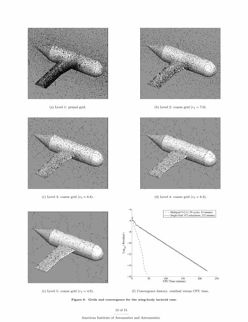
(a) Level 1: primal grid. (b) Level 2: coarse grid (r1 = 7.0).

(c) Level 3: coarse grid (r2 = 6.8). (d) Level 4: coarse grid (r3 = 6.2).

(e) Level 5: coarse grid (r4 = 4.9).

0 50 100 150 200 250−16

−14

−12

−10

−8

−6

−4

CPU Time (minute)

Log

10 (

Res

idua

l )

Multigrid V(2,1): 50 cycles, 43 minutesSingle Grid: 472 relaxations, 222 minutes

(f) Convergence history: residual versus CPU time.

Figure 6. Grids and convergence for the wing-body inviscid case.

12 of 15

American Institute of Aeronautics and Astronautics

(a) Level 1: primal grid. (b) Level 2: coarse grid (r1 = 5.9).

(c) Level 3: coarse grid (r2 = 5.1). (d) Level 4: coarse grid (r3 = 4.4).

(e) Level 5: coarse grid (r4 = 3.8).

0 20 40 60 80 100 120 140−16

−15

−14

−13

−12

−11

−10

−9

−8

−7

−6

CPU Time (minute)

Log

10 (

Res

idua

l )

Multigrid V(2,1): 66 cycles, 67 minutesSingle Grid: 236 relaxations, 127 minutes

(f) Convergence history: residual versus CPU time.

Figure 7. Grids and convergence for the wing-flap inviscid case.

13 of 15

American Institute of Aeronautics and Astronautics

(a) Level 1: primal grid. (b) Level 2: coarse grid (r1 = 6.3).

(c) Level 3: coarse grid (r2 = 5.6). (d) Level 4: coarse grid (r3 = 4.3).

(e) Level 5: coarse grid (r4 = 3.3).

0 20 40 60 80 100 120−9.5

−9

−8.5

−8

−7.5

−7

−6.5

−6

−5.5

CPU Time (minute)

Log

10 (

Res

idua

l )

Multigrid V(2,1): 23 cycles, 42 minutesSingle Grid: 122 relaxations, 116 minutes

(f) Convergence history: residual versus CPU time.

Figure 8. Grids and convergence for the NACA15-wing inviscid case.

14 of 15

American Institute of Aeronautics and Astronautics

0 5 10 15−5.5

−5

−4.5

−4

−3.5

−3

−2.5

−2

−1.5

−1

CPU Time (hour)

Log

10 (

Res

idua

l )

Multigrid V(2,1): 67 cycles, 3.0 hoursSingle−Grid: 590 relaxations, 14.9 hours

Figure 9. Residual versus CPU time for the F6 wing-body case (RANS).

15 of 15

American Institute of Aeronautics and Astronautics