Developable Surface Fitting to Point Clouds

Martin Peternell Computer Aided Geometric

Design 21(2004) 785-803

Reporter: Xingwang ZhangJune 19, 2005

About Martin Peternell

Affiliation Institute of Discrete Mathematics and Geometry Vienna University of Technology

Web http://www.geometrie.tuwien.ac.at/peternell

People Helmut Pottmann Johannes Wallner etc.

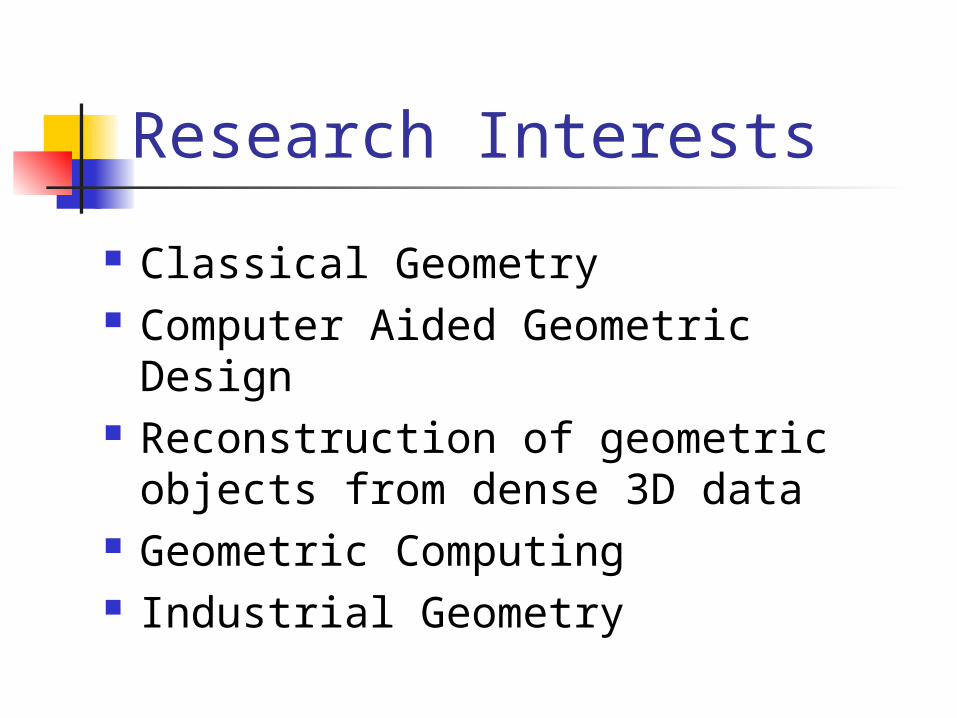
Research Interests

Classical Geometry Computer Aided Geometric

Design Reconstruction of geometric

objects from dense 3D data Geometric Computing Industrial Geometry

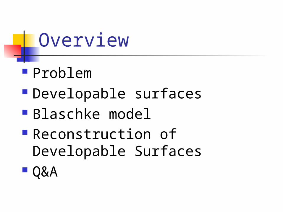
Overview

Problem Developable surfaces Blaschke model Reconstruction of Developable

Surfaces Q&A

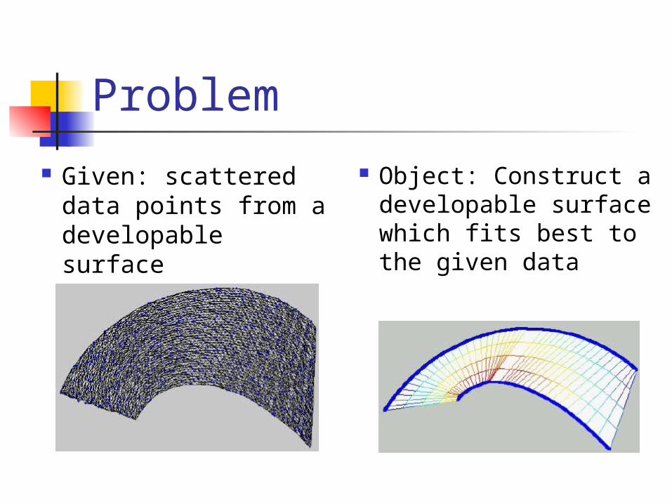
Problem

Given: scattered data points from a developable surface

Object: Construct a developable surface which fits best to the given data

Ruled Surface( , ) ( ) ( )u v u v u x c e

directrix curve ( ) :ue

( ) :uc

a

generator

A ruled surface

Normal vector

( , ) ( ) ( ) ( ) ( )u v u u v u u n c e e e

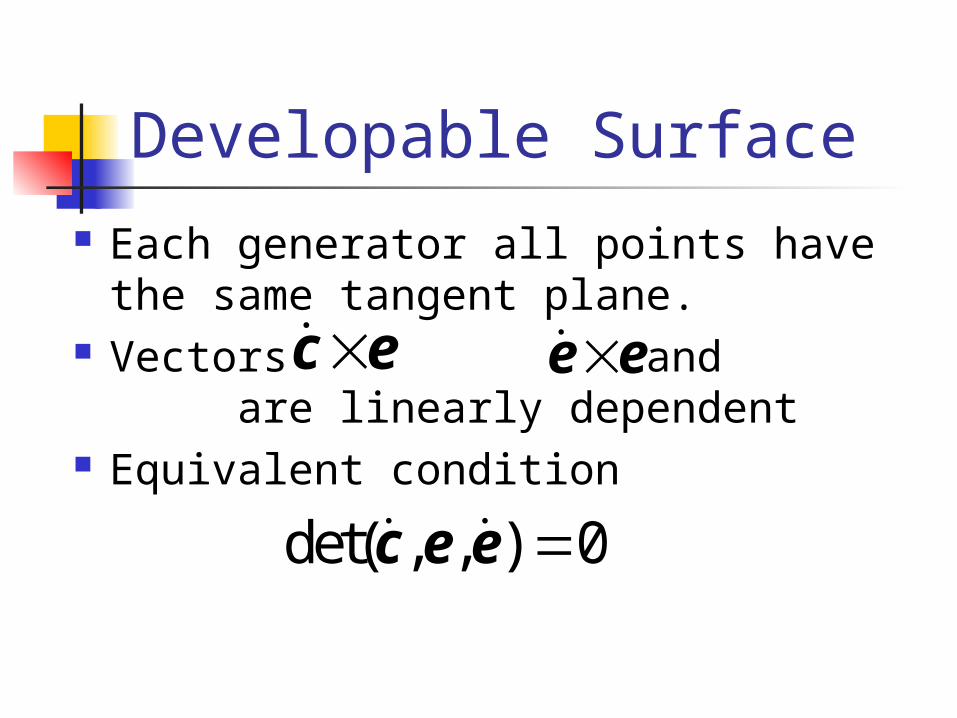
Developable Surface Each generator all points have the

same tangent plane. Vectors and are

linearly dependent Equivalent condition

c e e e

det( , , ) 0c e e

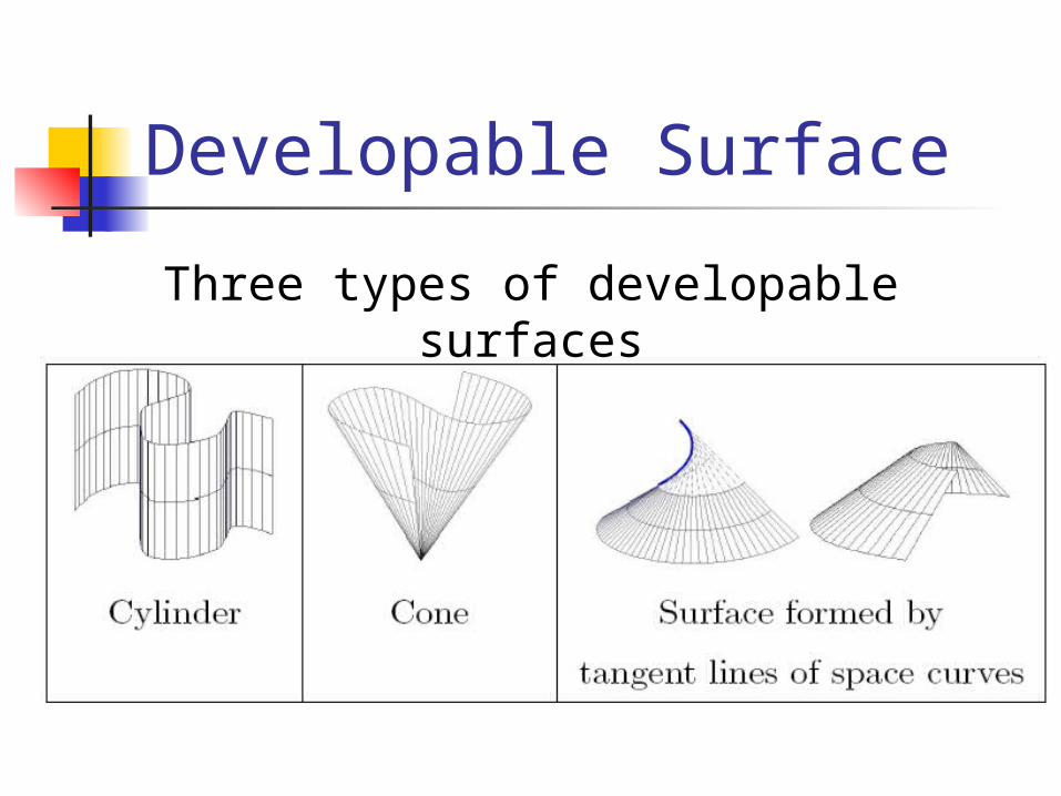
Developable Surface

Three types of developable surfaces

Geometric Properties of Developable Surface

Gaussian curvature is zero Envelope of a one-parameter

family of planes

Dual approach: is a curve in dual projective 3-space.

4 1 2 3( ) : ( ) ( ) ( ) ( ) 0u n u n u x n u y n u z T

( )uT

Singular Point A singular point doesn’t possess a

tangent plane. Singular curve is

determined by the parameter( ) ( , )su u vs x

2

( ) ( ).

( )sv

c e e e

e e

Three Different Classes

Cylinder: singular curve degenerates to a single point at infinity

Cone: singular curve degenerates to a single proper point, called vertex

Tangent surface: tangent lines of a regular space curve, called singular curve

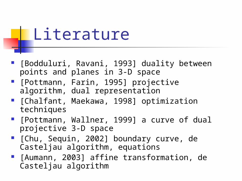
Literature

[Bodduluri, Ravani, 1993] duality between points and planes in 3-D space

[Pottmann, Farin, 1995] projective algorithm, dual representation

[Chalfant, Maekawa, 1998] optimization techniques [Pottmann, Wallner, 1999] a curve of dual

projective 3-D space [Chu, Sequin, 2002] boundary curve, de Casteljau

algorithm, equations [Aumann, 2003] affine transformation, de Casteljau

algorithm

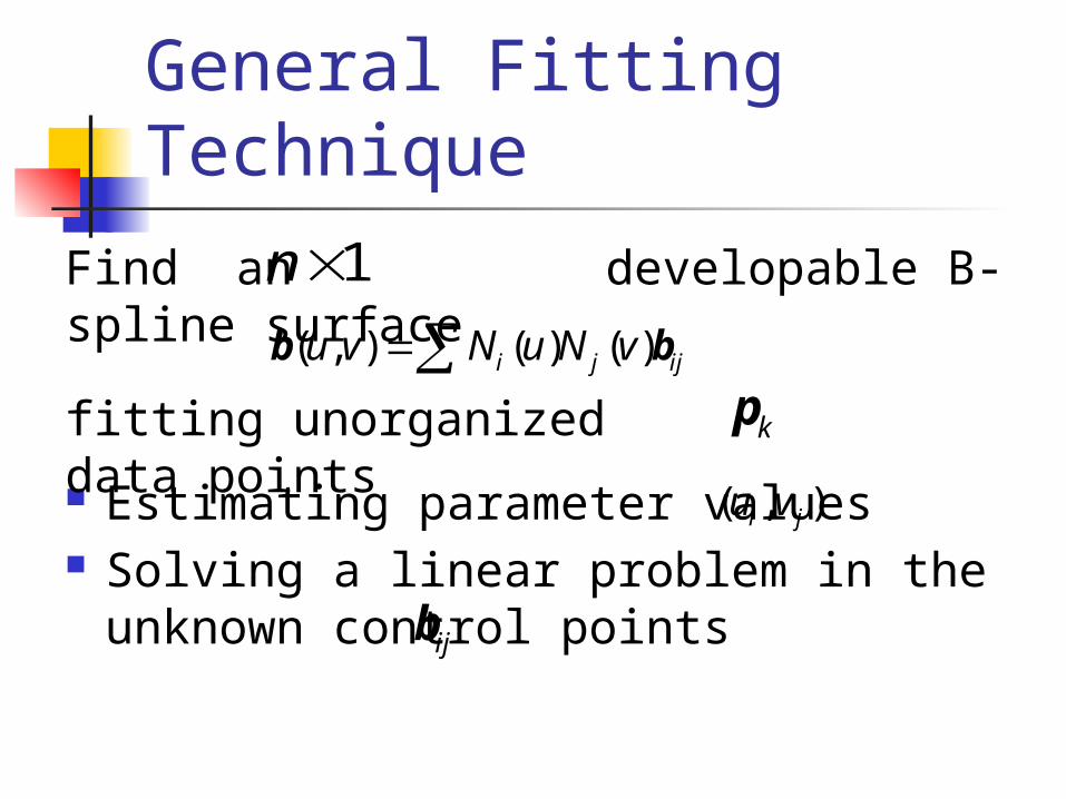
General Fitting Technique

Estimating parameter values Solving a linear problem in the

unknown control points

fitting unorganized data points

Find an developable B-spline surface

1n( , ) ( ) ( )i j iju v N u N vb b

kp

( , )i ju v

ijb

Two Difficult Problems Sorting scattered data

Estimation of data parameters Estimation of approximated direction

of the generating lines Guaranteeing resulting fitted

surface is developable Leading a highly non-linear side

condition in the control points

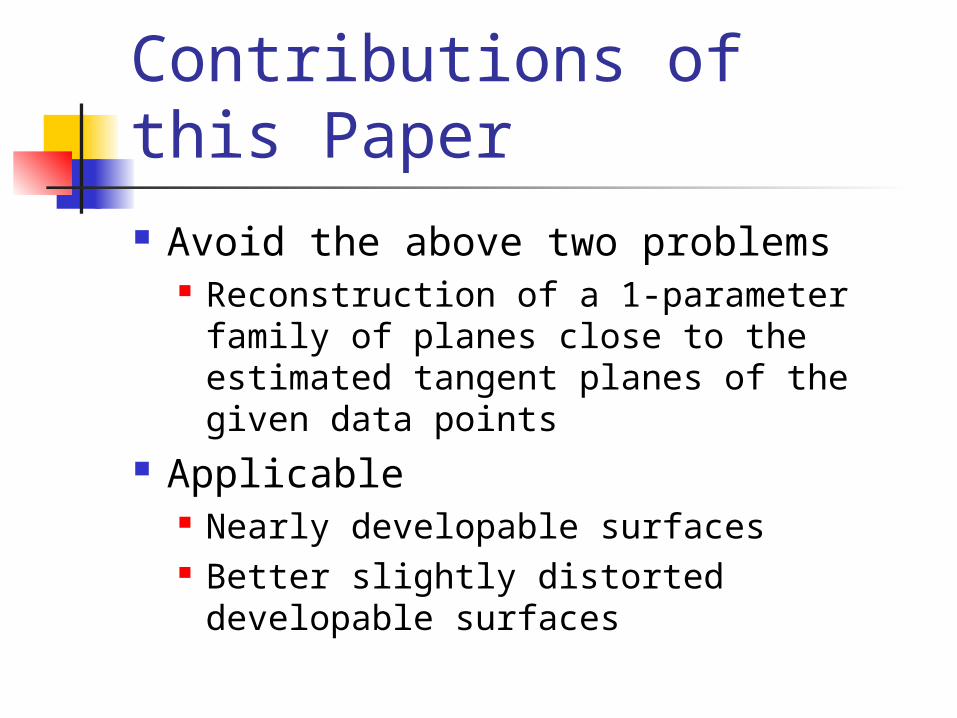
Contributions of this Paper Avoid the above two problems

Reconstruction of a 1-parameter family of planes close to the estimated tangent planes of the given data points

Applicable Nearly developable surfaces Better slightly distorted developable

surfaces

Blaschke Model

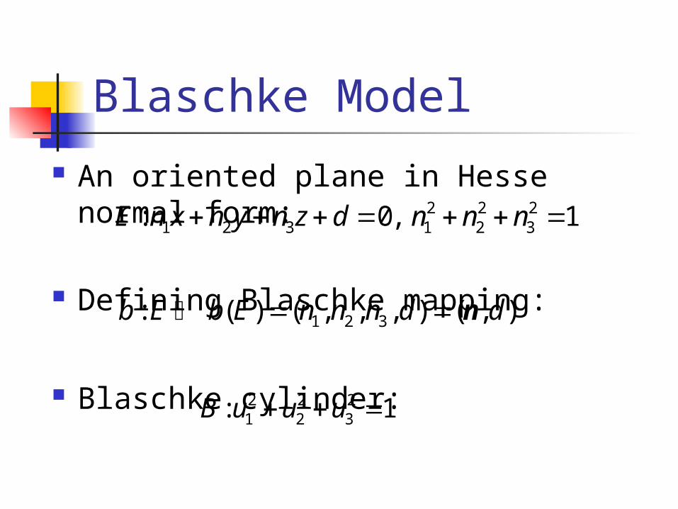
Blaschke Model

An oriented plane in Hesse normal form:

Defining Blaschke mapping:

Blaschke cylinder:

2 2 21 2 3 1 2 3: 0, 1E n x n y n z d n n n

1 2 3: ( ) ( , , , ) ( , )b E b E n n n d d n

2 2 21 2 3: 1B u u u

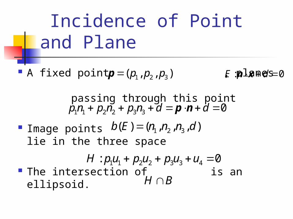
Incidence of Point and Plane

A fixed point , planes passing through this point

Image points lie in the three space

The intersection of is an ellipsoid.

1 2 3( , , )p p pp : 0E d n x

1 1 2 2 3 3 0p n p n p n d d p n

1 2 3( ) ( , , , )b E n n n d

1 1 2 2 3 3 4: 0H p u p u p u u

H B

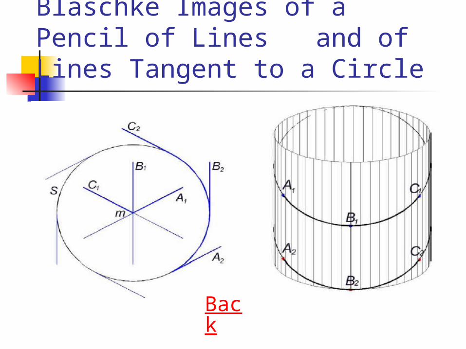
Blaschke Images of a Pencil of Lines and of Lines Tangent to a Circle

Back

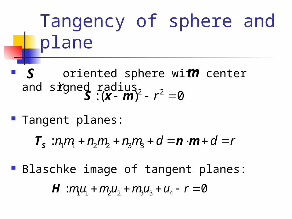
Tangency of sphere and plane

oriented sphere with center and signed radius

Tangent planes:

Blaschke image of tangent planes:

S mr 2 2: ( ) 0r S x m

1 1 2 2 3 3: n m n m n m d d r ST n m

1 1 2 2 3 3 4: 0mu m u m u u r H

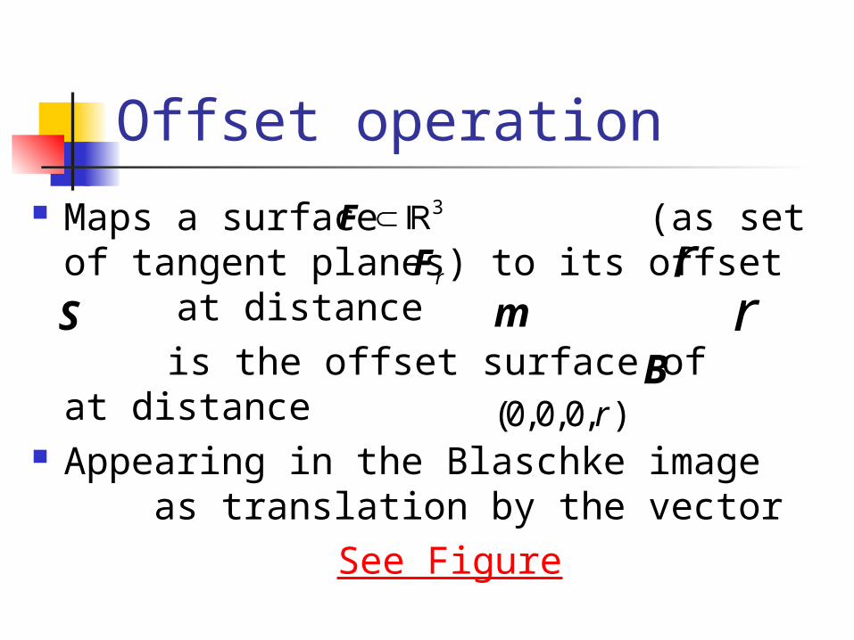
Offset operation Maps a surface (as set of

tangent planes) to its offset at distance

is the offset surface of at distance Appearing in the Blaschke image as

translation by the vector See Figure

3F

rF rS m r

B(0,0,0, )r

Laguerre Geometry satisfy :

inverse Blaschke image tangent to a sphere

form a constant angle with the direction vector

1 2 3 4( , , , )q q q q q B

0 1 1 2 2 3 3 4 4: 0a u a u a u a u a H

1( )bT = q

4 0.a

4 0.a

01 2 3

4 4

1( , , ),

aa a a r

a a m

T

T1 2 3( , , )a a aa =

The Tangent Planes of a Developable Surface

be a 1-parameter family of planes

Generating lines: Singular curve: Blaschke image is a curve

on the Blaschke cylinder

( )uT

4 1 2 3( ) : ( ) ( ) ( ) ( ) 0u n u n u x n u y n u z T

( ) ( ) ( ) ( )u u u u L T T T

( ) ( ) ( )u u u L T T

( ) ( )b u b DT

B

Classification

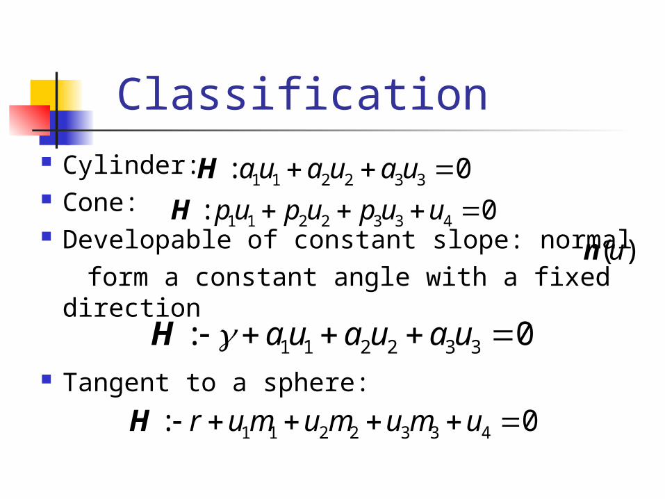
Classification Cylinder: Cone: Developable of constant slope: normal form a constant angle with a fixed

direction Tangent to a sphere:

1 1 2 2 3 3: 0a u a u a u H

1 1 2 2 3 3 4: 0p u p u p u u H

1 1 2 2 3 3: 0a u a u a u H

( )un

1 1 2 2 3 3 4: 0r u m u m u m u H

Recognition of Developable Surfaces from Point Clouds

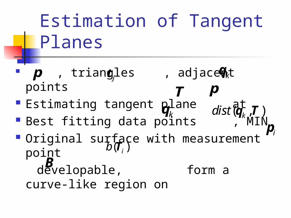
Estimation of Tangent Planes

, triangles , adjacent points Estimating tangent plane at Best fitting data points , MIN Original surface with measurement

point developable, form a curve-like

region on

p jt kq

T p

kq ( , )kdist q T

ip( )ib T

B

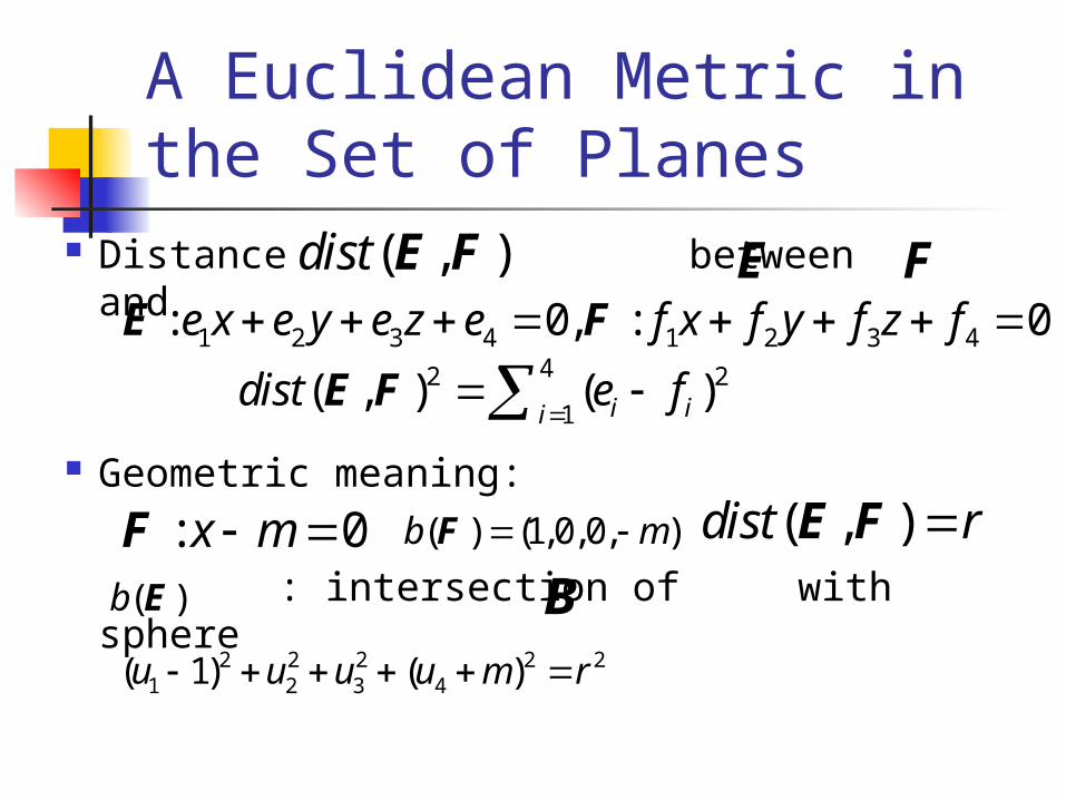
A Euclidean Metric in the Set of Planes

Distance between and

Geometric meaning:

: intersection of with sphere

( , )dist E F E F1 2 3 4 1 2 3 4: 0, : 0e x e y e z e f x f y f z f E F

42 2

1( , ) ( )i ii

dist e f

E F

: 0x m F ( ) (1,0,0, )b m F ( , )dist rE F

( )b E

2 2 2 2 21 2 3 4( 1) ( )u u u u m r

B

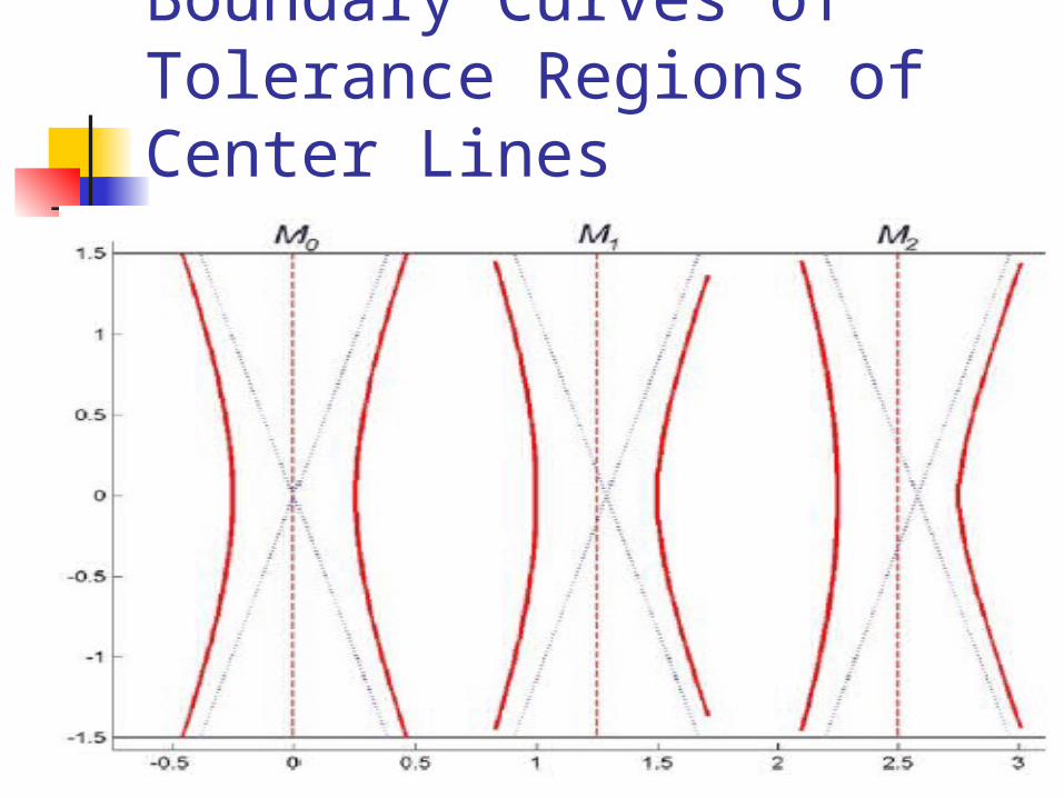
Boundary Curves of Tolerance Regions of Center Lines

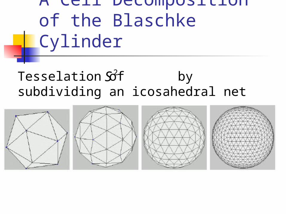
A Cell Decomposition of the Blaschke Cylinder

Tesselation of by subdividing an icosahedral net

2S

A Cell Decomposition of the Blaschke Cylinder (continued)

Cell structure on the Blaschke cylinder 20 triangles, 12 vertices, 2 intervals 80 triangles, 42 vertices, 4 intervals 320 triangles, 162 vertices, 8 intervals 1280 triangles, 642 vertices, 16 intervals

B

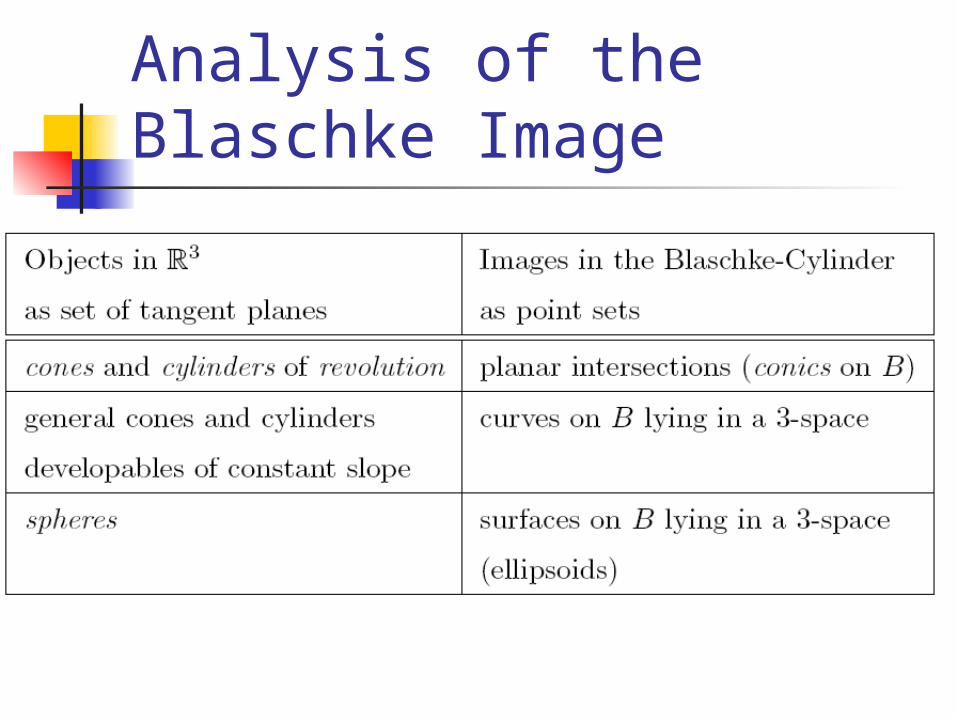
Analysis of the Blaschke Image

Analysis of the Blaschke Image (continued)

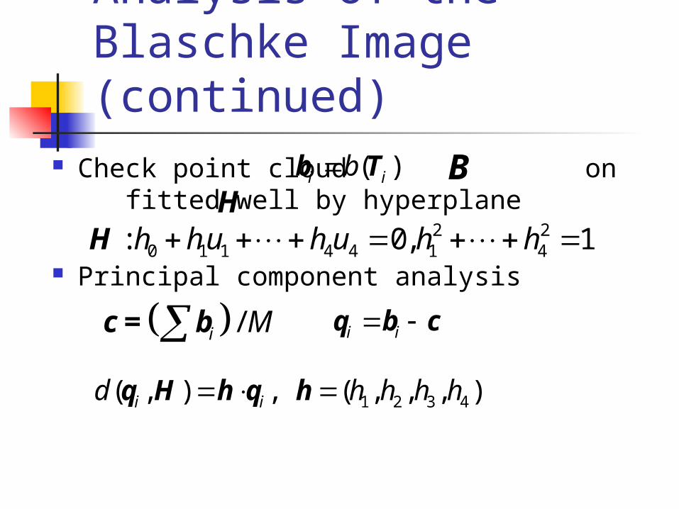
Check point cloud on fitted well by hyperplane

Principal component analysis

( )i ibb T BH

2 20 1 1 4 4 1 4: 0, 1h hu h u h h H

/i Mc = b i i q b c

1 2 3 4( , ) , ( , , , )i id h h h h q H h q h

Principal Component Analysis (continued)

Minimization

Eigenvalue problem

2 21 2 3 4

1 1

1 1( , , , ) ( , ) ( )

M M

i ii i

F h h h h dM M

q H h q

1

1( ) , :

MT T

i ii

F C CM

h h h q q

1 2 3 4Deviations: 1 2 3 4Eigenvalues:

Principal Component Analysis (continued)

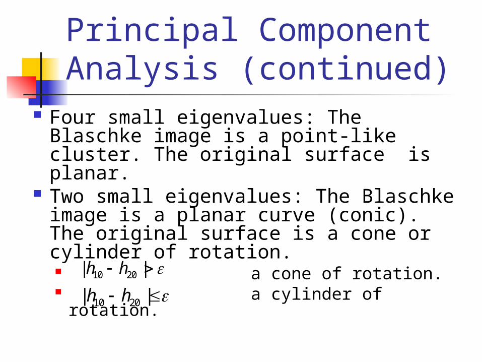
Four small eigenvalues: The Blaschke image is a point-like cluster. The original surface is planar.

Two small eigenvalues: The Blaschke image is a planar curve (conic). The original surface is a cone or cylinder of rotation. a cone of rotation. a cylinder of rotation.

10 20| |h h

10 20| |h h

Principal Component Analysis (continued)

One small eigenvalue and curve-like Blaschke image. The original surface is developable. a general cone a general cylinder a developable of constant slope.

One small eigenvalue and surface-like Blaschke-image: The original surface is a sphere.

10| |h

14| |h 10 14| | ,| |h h

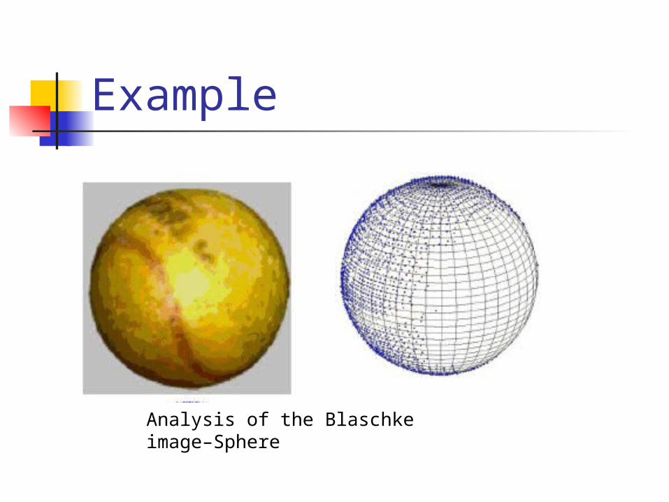
Example

Analysis of the Blaschke image–Sphere

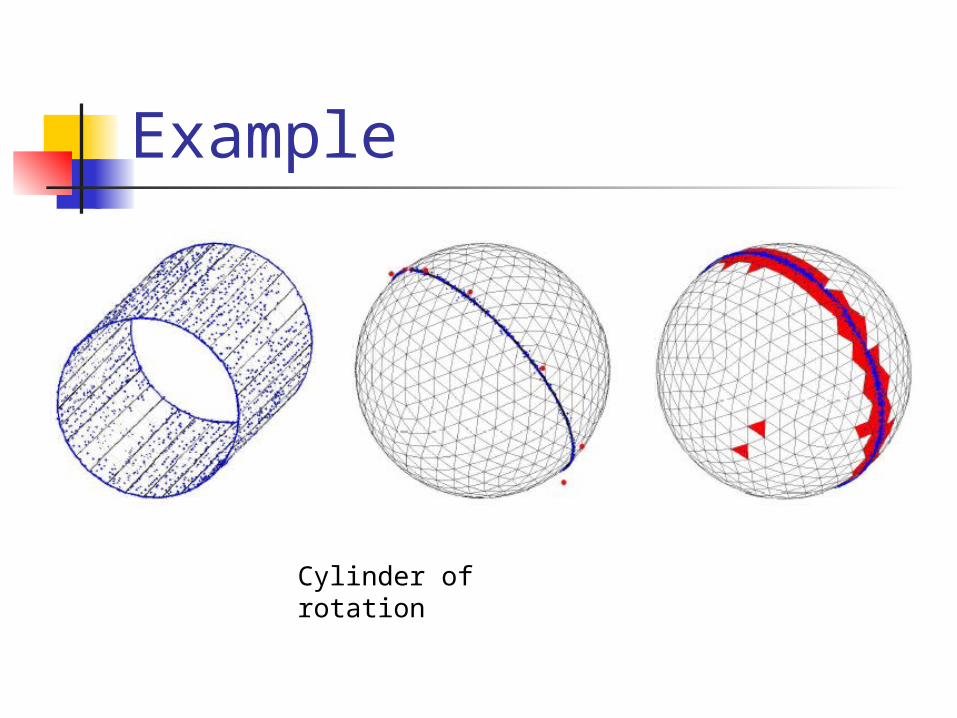
Example

Cylinder of rotation

Example

Approximation of a developable of constant slope

Example

General cylinder

Triangulated data points and approximation

Original Blaschke image

Example

Developable of constant slope

Triangulated data points and approximation

Spherical image of the approximation with control points.

Reconstruction of Developable Surfaces from Measurements

Reconstruction Find a curve fitting best the

tubular region defined by Determine 1-parameter family of

tangent planes determined by Compute a point-representation of the

corresponding developable approximation of the data points

( )ib T

D*

( )t c B

( )tc( )tE

Parametrizing a Tubular Region

Determine relevant cells of carrying points

Thinning of the tubular region: Find cells carrying only few points and delete these cells and points

Estimate parameter values for a reduced set of points (by moving least squares: marching through the tube)

Compute an approximating curve on w.r.t. points

( , , , )i i i i ia b c dC

B

kC

( )tc BkC

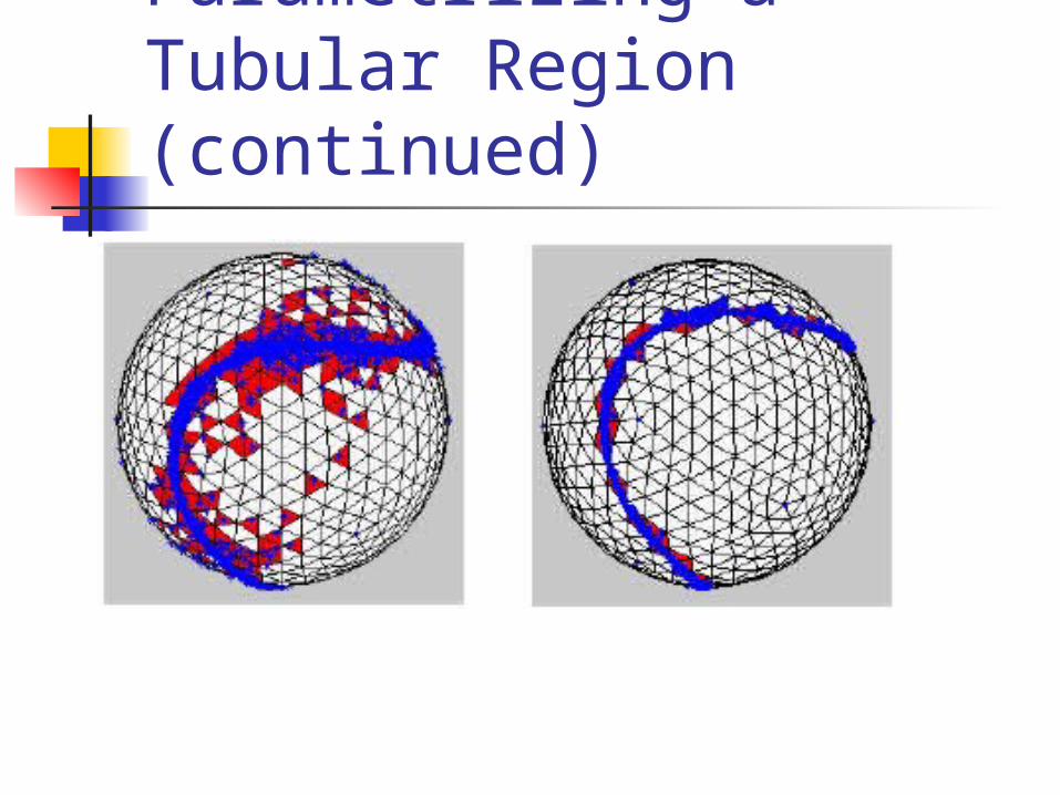
Parametrizing a Tubular Region (continued)

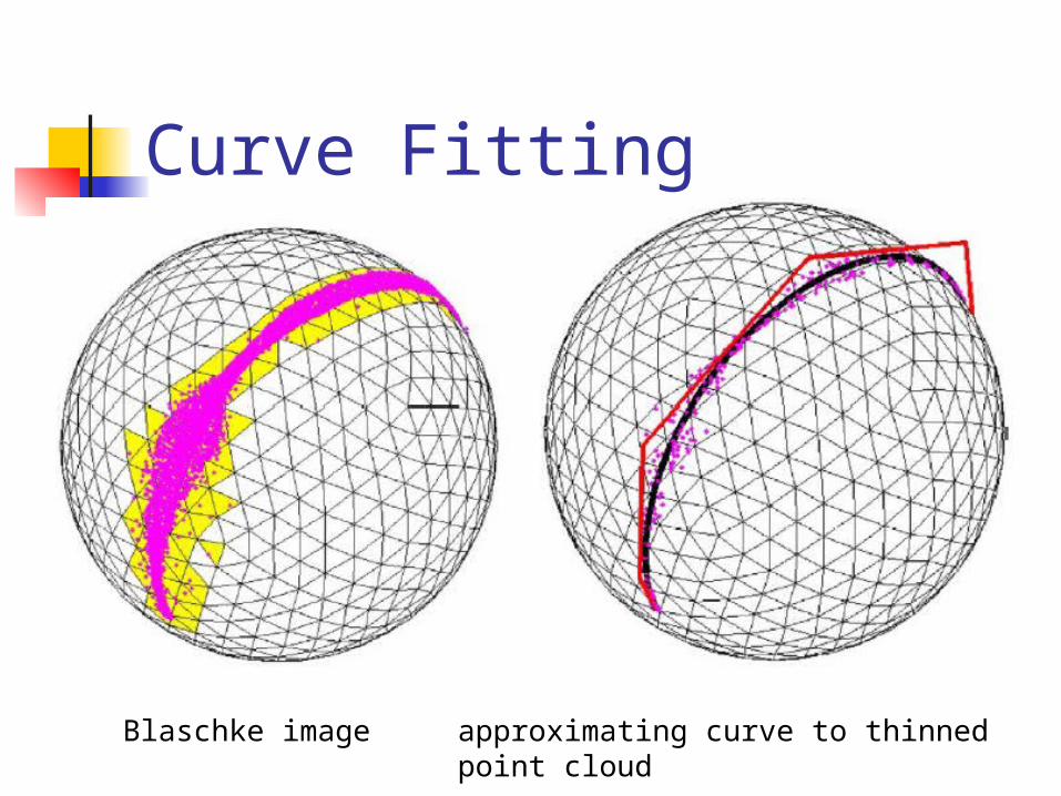
Curve Fitting

Blaschke image approximating curve to thinned point cloud

Curve Fitting (continued)

support function (fourth coordinate)

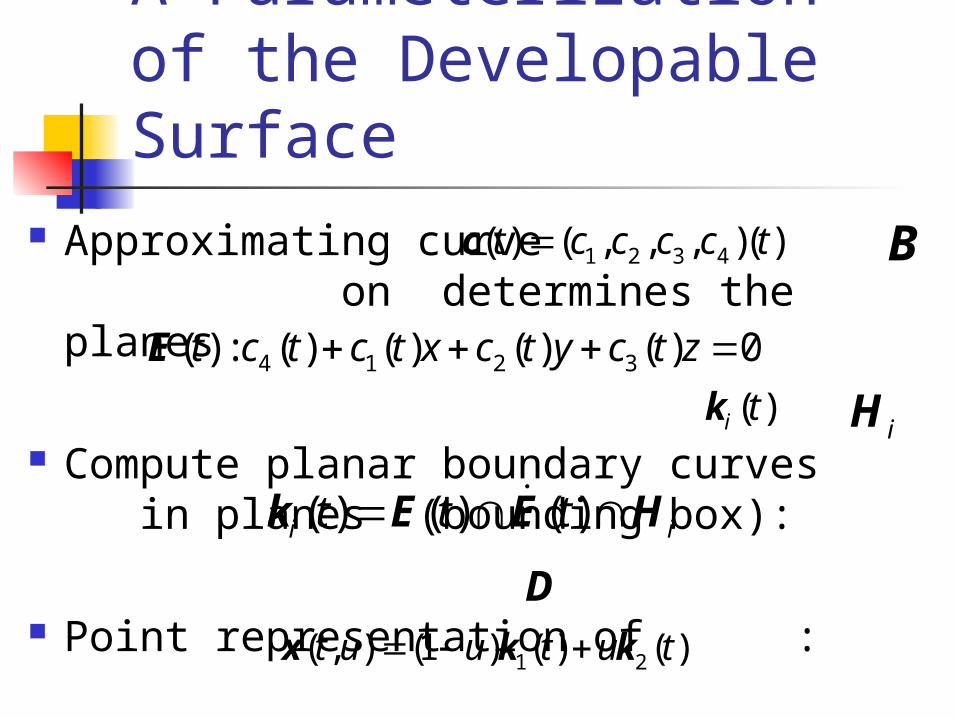
A Parameterization of the Developable Surface

Approximating curve on determines the planes

Compute planar boundary curves in planes (bounding box):

Point representation of :

( ) ( ) ( )i it t t k E E H

4 1 2 3( ) : ( ) ( ) ( ) ( ) 0t c t c t x c t y c t z E

1 2 3 4( ) ( , , , )( )t c c c c tc B

( )i tkiH

D

1 2( , ) (1 ) ( ) ( )t u u t u t x k k

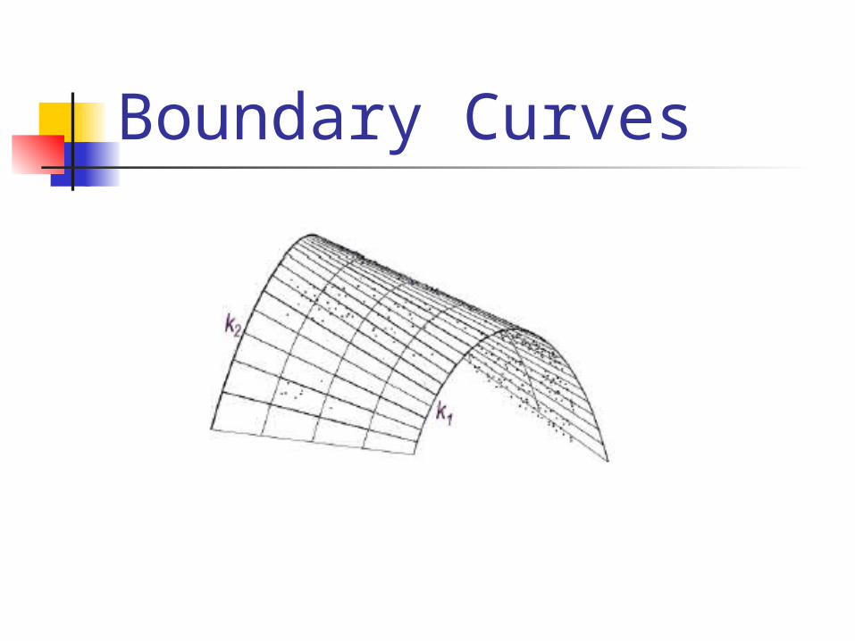
Boundary Curves

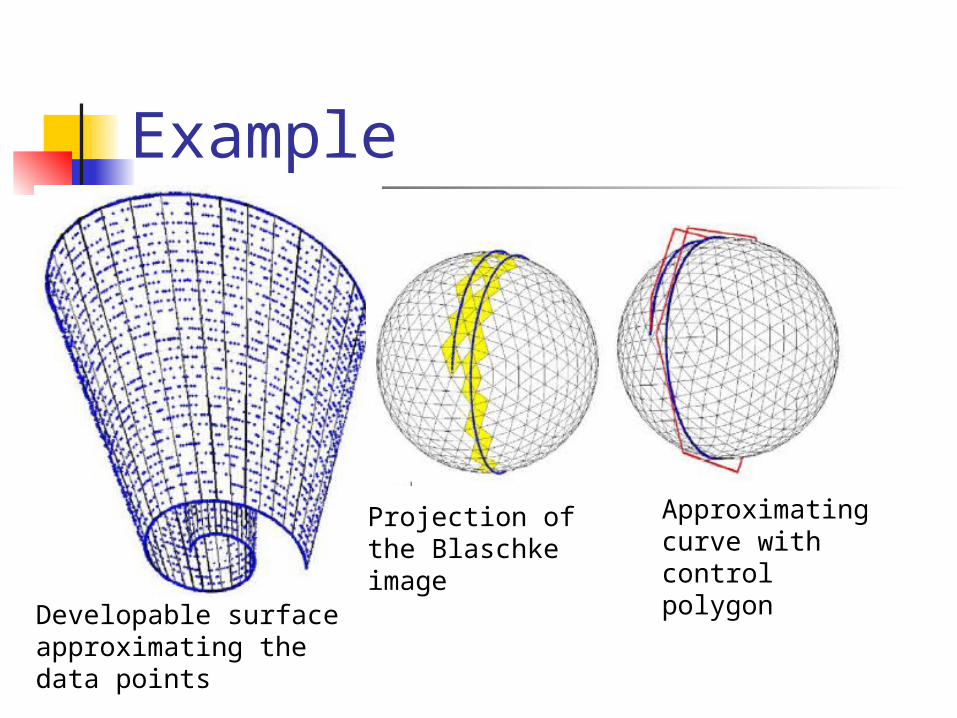
Example

Developable surface approximating the data points

Projection of the Blaschke image

Approximatingcurve with control polygon

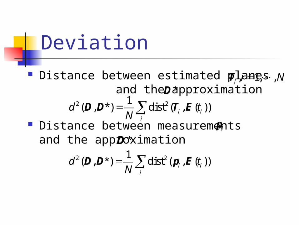
Deviation Distance between estimated planes

and the approximation

Distance between measurements and the approximation

2 21( , *) dist ( , ( ))i i

i

d tN

D D p E

2 21( , *) dist ( , ( ))i i

i

d tN

D D T E

, 1, ,i i N T*D

ip

*D

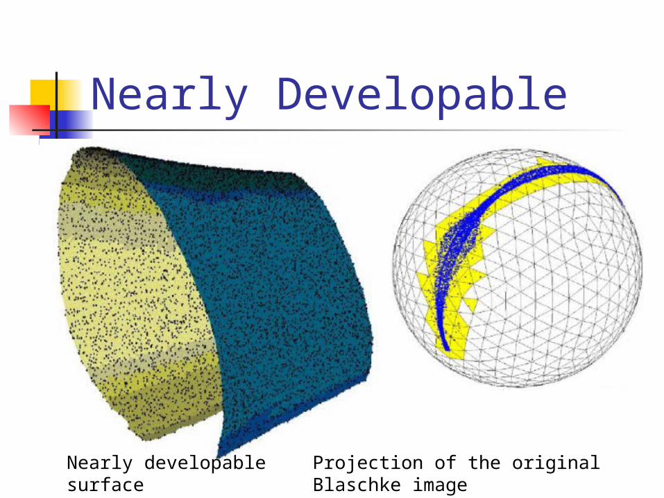
Nearly Developable

Nearly developable surface

Projection of the original Blaschke image

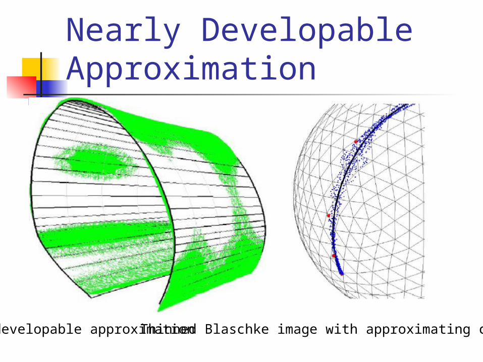
Nearly Developable Approximation

developable approximationThinned Blaschke image with approximating curve

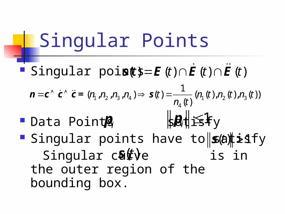
Singular Points Singular points

Data Points satisfy Singular points have to satisfy Singular curve is in the outer

region of the bounding box.

( ) ( ) ( ) ( )t t t t s E E E

1 2 3 4 1 2 34

1( , , , ) ( ) ( ( ), ( ), ( ))

( )n n n n t n t n t n t

n t n c c c = s

ip 1i p( ) 1t s

( )ts

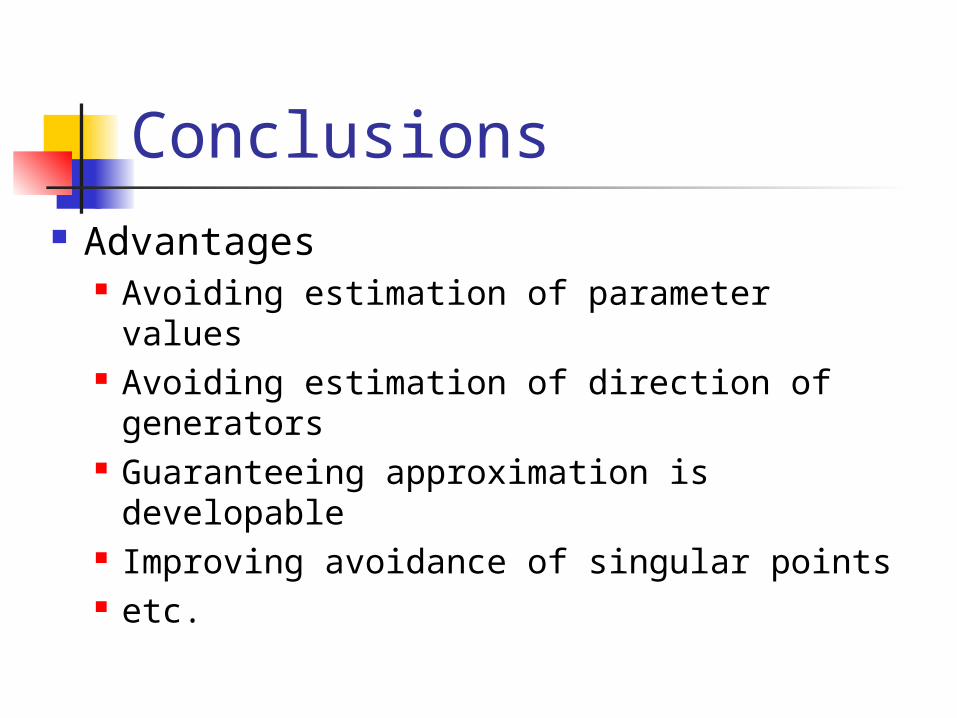
Conclusions Advantages

Avoiding estimation of parameter values Avoiding estimation of direction of

generators Guaranteeing approximation is

developable Improving avoidance of singular points etc.

Q&A

Questions?

Thanks all!Thanks all!Especial Especial

thanks to Dr thanks to Dr Liu’s helpLiu’s help

Thanks all!Thanks all!Especial Especial

thanks to Dr thanks to Dr Liu’s helpLiu’s help