Determinants of Income Generating Activities of Rural - eDiss
146
Determinants of Income Generating Activities of Rural Households A Quantitative Study in the Vicinity of the Lore-Lindu National Park in Central Sulawesi/Indonesia Dissertation zur Erlangung des Doktorgrades der Fakultät für Agrarwissenschaften der Georg-August-Universität Göttingen vorgelegt von Stefan Schwarze geboren in Frankfurt/Main Göttingen, April 2004
Transcript of Determinants of Income Generating Activities of Rural - eDiss
Determinants of Income Generating Activities
of Rural Households
A Quantitative Study in the Vicinity of
the Lore-Lindu National Park in
Central Sulawesi/Indonesia
Dissertation
zur Erlangung des Doktorgrades
der Fakultät für Agrarwissenschaften
der Georg-August-Universität Göttingen
vorgelegt von
Stefan Schwarze
geboren in Frankfurt/Main
Göttingen, April 2004
II
D7
1. Referent: Prof. Dr. Manfred Zeller
2. Referent: Prof. Dr. Hermann Waibel
Tag der mündlichen Prüfung: 27.05.2004
Autor:
Stefan Schwarze
Diplom-Agraringenieur
Contact:
Institute of Rural Development
Georg-August-University of Göttingen
Waldweg 26
37073 Göttingen
Phone: ++49-551-393915
Fax: ++49-551-393076
Email: [email protected]
Abstract
This study aims to identify and analyse the determinants of income generating
activities of rural households in the vicinity of the Lore-Lindu National Park in Cen-
tral Sulawesi, Indonesia. It helps to identify factors which are essential for the design
of policies promoting alternative income strategies. Data was collected through a
standardised, formal questionnaire from 301 randomly selected households. In the
analysis, the following income generating activities are differentiated: agricultural
self-employment, agricultural wage labour, non-agricultural self-employment, and
non-agricultural wage labour. Because of its importance the agricultural self-
employment category is further divided into annual and perennial crop production,
livestock production, and the sale of forest products. Various econometric models are
used to analyse the influence of socio-economic factors on income generating activi-
ties. A linear model is applied in the case of total household income. Probit models
are used to investigate factors influencing activity choice. In the analysis of activity
incomes, a simultaneous equation model with correction for the endogeneity of activ-
ity choice is applied. Finally, the determinants of income diversification are analysed
using Tobit models.
Abstract IV
Agricultural activities are the most important source of income for rural
households in the region and make up 70% of total household income. Within this
category the most important source of income is crop production, with the most im-
portant crops being irrigated rice and cocoa. The remaining 30% of the total house-
hold income originates from non-agricultural activities. However, only around 18%
of the households gain income from the latter activities. In contrast, 96% participate
in agricultural activities. Differentiation between different wealth groups shows that
activities outside the agricultural sector are particularly important for the less-poor
households. Although rural households are engaged in many different activities,
there exists a specialisation among households. Applying a Lorenz curve shows a
rather uneven distribution of income among households.
The econometric analysis shows that access to physical and human capital has
a significant influence on total household income. The area owned, the value of other
assets possessed, as well as the number of livestock and family labourers positively
influence household income. The possession of land also has a strong positive influ-
ence on the participation in crop production, whereas the possession of irrigated land
reduces the likelihood of participation in agricultural wage labour activities and in
the sale of forest products. Richer and non-indigenous households are more likely to
participate in non-agricultural self-employment. In contrast, non-indigenous house-
holds are less likely to participate in the sale of forest products and in agricultural
wage labour activities. Participation in formal credit markets discourages participa-
tion in annual crop production, but encourages participation in the production of per-
ennial crops and non-agricultural wage labour activities. The access to roads has a
strong influence on participation in almost all activities. The analysis of activity in-
comes shows again that the possession of land has a strong positive influence on the
income gained from crop production, while the possession of irrigated land reduces
the income gained from agricultural wage labour and the sale of forest products.
Similar to its effect on participation, the value of other assets owned has a positive
influence on the income from non-agricultural self-employment. The analysis also
shows the importance of education in non-agricultural wage labour activities and in
annual crop production. Ethnicity has a strong influence on perennial crop produc-
Abstract V
tion as well as on income from non-agricultural self-employment. The access to tar-
mac roads has a positive effect on the income from agricultural wage labour and the
sale of forest products. Diversification out of the agricultural sector is positively in-
fluenced by the wealth of the household, education, and participation in formal credit
markets. The number of livestock owned and the access to social capital have a posi-
tive effect on the overall degree of diversification.
The results of the analysis are used to draw policy conclusions with respect to
poverty alleviation, deforestation and rural development.
Zusammenfassung
Die vorliegende Dissertation untersucht den Einfluss sozioökonomischer Fak-
toren auf die Einkommensaktivitäten ländlicher Haushalte in der Umgebung des Lo-
re-Lindu-Nationalparks in Zentralsulawesi, Indonesien. Die Kenntnis dieser Faktoren
ist Voraussetzung für die Formulierung von Politikmaßnahmen und Entwicklungs-
projekten, die der Schaffung alternativer Einkommensmöglichkeiten dienen. Die
Datengrundlage bildet eine Befragung von 301 zufällig ausgewählten Haushalten
mittels Fragebögen. In der Analyse wird selbständige Tätigkeit sowie Lohnarbeit im
beziehungsweise außerhalb des landwirtschaftlichen Sektors unterschieden. Auf-
grund ihrer Bedeutung wird die selbständige Tätigkeit im Agrarsektor untergliedert
in die Produktion ein- und mehrjähriger Kulturen, die Tierproduktion, und in den
Verkauf von Produkten, die im Wald gesammelt wurden. In der ökonometrischen
Modellierung kommen lineare, Probit sowie Tobit Modelle zur Anwendung. Außer-
dem wird in der Analyse des Einkommens aus den einzelnen Aktivitäten ein simul-
tanes Gleichungsmodel mit Korrektur der Endogenität der Aktivitätenwahl ange-
wendet.
Zusammenfassung VII
Tätigkeiten im landwirtschaftlichen Sektor tragen 70% zum gesamten Haus-
haltseinkommen bei. Innerhalb dieses Sektors stammen 60% des Einkommens aus
der Pflanzenproduktion, wobei Nassreis und Kakao die bedeutendsten Kulturen sind.
Aktivitäten außerhalb des landwirtschaftlichen Sektors tragen 30% zum Haus-
haltseinkommen bei und sind besonders bedeutsam für die bessergestellten Haushal-
te. Allerdings erzielen nur 18% aller Haushalte überhaupt Einkommen aus diesen
Aktivitäten, wohingegen 96% der Haushalte Einkommen aus Tätigkeiten im land-
wirtschaftlichen Sektor haben. Obwohl Haushalte in vielen verschiedenen Aktivitä-
ten involviert sind, gibt es doch eine Spezialisierung hinsichtlich einer Einkommens-
aktivität.
Die ökonometrische Analyse zeigt, dass insbesondere die Ausstattung an
physischem Kapital sowie an Humankapital das Gesamthaushaltseinkommen positiv
beeinflusst. Die Analyse der Einkommensaktivitäten ist untergliedert in die Untersu-
chung der Entscheidung zur Teilnahme an Aktivitäten und der Höhe des daraus er-
zielten Einkommens. Der Besitz an Bewässerungsland wirkt negativ auf die Teil-
nahme an landwirtschaftlicher Lohnarbeit und den Verkauf von Waldprodukten.
Reichere Haushalte nehmen mit einer höheren Wahrscheinlichkeit an selbständiger
Tätigkeit außerhalb des landwirtschaftlichen Sektors teil. Das gleiche trifft auf nicht-
indigene im Vergleich zu indigenen Haushalten zu. Jedoch nehmen nicht-indigene
Haushalte mit geringerer Wahrscheinlichkeit am Verkauf von Waldprodukten und an
landwirtschaftlicher Lohnarbeit teil. Die Aufnahme von Krediten von formellen In-
stitutionen erhöht die Wahrscheinlichkeit der Produktion mehrjähriger Kulturen und
der Teilnahme an Lohnarbeit außerhalb des landwirtschaftlichen Sektors. Im Gegen-
satz dazu reduziert der Zugang zu Krediten die Teilnahme an der Produktion einjäh-
riger Kulturen. Die Analyse des erzielten Einkommens aus den einzelnen Aktivitä-
ten zeigt den starken positiven Einfluss von Landbesitz auf das erzielte Einkommen
aus der Pflanzenproduktion. Darüber hinaus hat der Besitz von Bewässerungsland
einen negativen Einfluss auf das Einkommen aus landwirtschaftlicher Lohnarbeit
sowie dem Verkauf von Waldprodukten. Reichere Haushalte nehmen nicht nur mit
höherer Wahrscheinlichkeit an selbständiger Tätigkeit außerhalb des landwirtschaft-
lichen Sektors teil, sie erzielen dort auch ein höheres Einkommen. Weiterhin zeigt
die ökonometrische Analyse die Bedeutung von Schulbildung auf das Einkommen
Zusammenfassung VIII
aus nicht-landwirtschaftlicher Lohnarbeit sowie der Produktion einjähriger Kulturen.
Nicht-indigene Haushalte erzielen höhere Einkommen aus der Produktion mehrjähri-
ger Kulturen und aus selbständiger Tätigkeit außerhalb des landwirtschaftlichen Sek-
tors. Die Entfernung zu Asphaltstraßen hat einen negativen Einfluss auf das Ein-
kommen aus landwirtschaftlicher Lohnarbeit sowie dem Verkauf von Waldproduk-
ten.
Diese Ergebnisse dienen zur Formulierung potentieller Politikmaßnahmen im
Hinblick auf Armutsreduzierung, Verringerung der Umwandlung von Wald in land-
wirtschaftliche Flächen sowie auf die Entwicklung des ländlichen Raumes.
Acknowledgments
This dissertation is the final result of four years of sometimes frustrating but
often very exciting work at the Institute of Rural Development (IRD) in Goettingen
and the STORMA project in Palu/Indonesia. During this time a large member of
people supported the development of this dissertation, making it impossible to name
them all.
I am grateful to Prof. Dr. Manfred Zeller, Professor at the Institute of Rural
Development of the University of Goettingen, for his supervision, guidance and sup-
port. He gave me the opportunity to work as a research associate at the IRD and
within an interdisciplinary research project. I have found this combination very excit-
ing. I would also like to thank my second supervisor, Prof. Dr. Hermann Waibel,
Professor at the Institute of Economics in Horticulture of the University of Hannover,
for his thorough and helpful evaluation of this dissertation.
I would like to address a word of gratitude to all members of the IRD and of
the STORMA project. I particularly have to thank Nunung Nuryartono, my friend
and STORMA colleague. Without him, the field research would have been impossi-
ble. In this regard, I am also grateful to our Indonesian students, who conducted the
Acknowledgments X
interviews: Januar, Pitono, Maskur, Akas, Ketut, Yonathan, Sumarno, Benyamin,
Umar, Sarton, Yasin, and Sukadarman. Furthermore, I have to thank all our respon-
dents for patiently answering our questions (two times almost 40 pages of ques-
tions!). I particularly appreciated the cooperation with Teunis van Rheenen, Miet
Maertens, Marhawati Mappatoba, and Regina Birner; all from the IRD and members
of STORMA. I would also like to thank Robert, Sylvia, Georg, and Frank for the fun
we have had in Palu. I am grateful to Abu Shaban for calculating the poverty index
used in this dissertation, Sebastian Hess and Ingrid Sander for supporting my work as
student assistants, and Orly Johansson for proofreading. I appreciated the collabora-
tion with my colleagues at the IRD, particularly Daniel Mueller, Maria Mañez Costa,
and Alwin Keil.
Last, but not least, I want to thank Christine, Lina, and Paula. This book is
dedicated to them!
Stefan Schwarze, Goettingen, May 2004
Table of Contents
Abstract...................................................................................................................... III
Zusammenfassung ..................................................................................................... VI
Acknowledgments ..................................................................................................... IX
Table of Contents....................................................................................................... XI
List of Tables .......................................................................................................... XIV
List of Figures.......................................................................................................XVIII
Abbreviations.......................................................................................................... XIX
1 Introduction ................................................................................................. 1
1.1 Background...................................................................................................1
1.2 The research area ..........................................................................................2
1.3 Problem analysis ...........................................................................................4
1.4 Objectives and research topics......................................................................5
1.5 Outline ..........................................................................................................5
2 Conceptual framework ................................................................................ 8
2.1 Conceptual approaches linking assets with activity choice and
incomes.........................................................................................................9
Table of Contents XII
2.2 Definition of income and its classification .................................................12
2.3 Review of empirical evidence on determinants influencing income
generating activities....................................................................................13
2.4 Mathematical model of activity choice and income ...................................16
2.5 Summary.....................................................................................................18
3 Methodology ............................................................................................. 20
3.1 Sampling frame and selection of households .............................................21
3.2 Data collection, entry, and cleaning............................................................24
3.3 Measurement of the dependent variables....................................................26
3.3.1 Measurement of income..................................................................... 26
3.3.2 Measuring income diversity............................................................... 28
3.4 Measurement of the independent variables ................................................29
3.4.1 Internal factors ................................................................................... 29
3.4.2 External factors .................................................................................. 31
3.5 Methodology used in the descriptive analysis ............................................32
3.6 Methodology used in the causal analysis....................................................35
3.6.1 Total household income..................................................................... 35
3.6.2 Participation in income activities....................................................... 37
3.6.3 Activity income.................................................................................. 37
3.6.4 Income diversity ................................................................................ 40
3.7 Summary.....................................................................................................41
4 Descriptive analysis of income and activities ........................................... 42
4.1 Income and activities ..................................................................................43
4.2 Agricultural self-employed income ............................................................46
4.2.1 Crop income....................................................................................... 47
4.2.2 Livestock income............................................................................... 48
4.2.3 Income from forest products.............................................................. 49
4.3 Self-employed income outside agriculture .................................................52
4.4 Agricultural wage labour income ...............................................................53
4.5 Non-agricultural wage labour income ........................................................56
4.6 Income shares and income specialisation ...................................................59
4.7 Income distribution .....................................................................................62
Table of Contents XIII
4.8 Summary.....................................................................................................63
5 Descriptive analysis of factors influencing income and activity choice ... 65
5.1 Physical capital ...........................................................................................66
5.1.1 Possession of land.............................................................................. 66
5.1.2 Other assets ........................................................................................ 72
5.2 Human capital .............................................................................................72
5.3 Social capital...............................................................................................75
5.4 Financial markets........................................................................................81
5.5 Road infrastructure .....................................................................................83
5.6 Summary.....................................................................................................84
6 Results of the econometric analysis .......................................................... 86
6.1 Total household income..............................................................................89
6.2 Participation by activity ..............................................................................90
6.3 Income by activity ......................................................................................95
6.4 Diversification ..........................................................................................100
6.5 Summary...................................................................................................103
7 Conclusions ............................................................................................. 105
7.1 Major results .............................................................................................106
7.2 Policy conclusions ....................................................................................107
8 References ............................................................................................... 111
9 Appendix ................................................................................................. 116

List of Tables
Table 1: Sample villages of STORMA and their sampling weights...........................24
Table 2: Livestock conversion factors ........................................................................30
Table 3: Income and participation by activity ............................................................43
Table 4: Income and participation by activity and poverty group..............................45
Table 5: Participation, share in gross income, share in input expenditures, and
share in net income by crop..........................................................................47
Table 6: Share in net income by crop and region .......................................................48
Table 7: Livestock income and participation by type.................................................49
Table 8: Collection and sale of rattan by poverty group.............................................51
Table 9: Income from forest products by region ........................................................51
Table 10: Self-employed income outside agriculture by activity ...............................52
Table 11: Self-employed income outside agriculture by region.................................53
Table 12: Distribution of workers, days employed, and income by agricultural
wage labour activity ...................................................................................54
Table 13: Distribution of workers and income from agricultural wage labour
activities by region .....................................................................................54
List of Tables XV
Table 14: Distribution of workers and income from agricultural wage labour
activities by age group and level of education ...........................................55
Table 15: Distribution of workers and income from agricultural wage labour
activities by gender.....................................................................................56
Table 16: Distribution of workers, days employed, and income by non-
agricultural wage labour activity .............................................................57
Table 17: Distribution of workers and income from non-agricultural wage
labour activities by region........................................................................57
Table 18: Distribution of workers and income from non-agricultural wage
labour activities by age group and level of education..............................58
Table 19: Distribution of workers and income from non-agricultural wage
labour activities by gender .......................................................................59
Table 20: Income shares by activity ...........................................................................60
Table 21: Income specialisation .................................................................................61
Table 22: Share of land owned by sub district............................................................66
Table 23: Share of land owned by type of land and sub district.................................67
Table 24: Share of agricultural land owned by type of land and sub district .............67
Table 25: Share of dryland owned by sub district ......................................................68
Table 26: Share of wetland owned by sub district......................................................69
Table 27: Share of wetland owned by type of irrigation ............................................70
Table 28: Share of land owned by type ......................................................................71
Table 29: Clustering of households according to the type of agricultural land
owned .........................................................................................................71
Table 30: Mean value of other assets owned by sub district ......................................72
Table 31: Household composition by sub district ......................................................73
Table 32: Level of education by sub district...............................................................74
Table 33: Education by gender ...................................................................................74
Table 34: Membership in organisations by sub district ..............................................75
Table 35: Most important organisations .....................................................................76
Table 36: Meeting attendance, activity in decision-making, and labour days
spent in the most important organisation ...................................................77
Table 37: Ethnic groups..............................................................................................78
List of Tables XVI
Table 38: Share of non-indigenous households by sub district ..................................78
Table 39: Share of migrant households by sub district...............................................79
Table 40: Share of migrant households by year of migration and sub district ...........80
Table 41: Share of migrant households by origin and sub district .............................80
Table 42: Share of households received loan by source and sub district ...................81
Table 43: Average loan received by source and sub district in IDR 1000 .................82
Table 44: Share used for agriculture by source and sub district .................................83
Table 45: Distance to tarmac road by sub district in walking hours...........................84
Table 46: Descriptive statistics of the dependent variables........................................87
Table 47: Descriptive statistics of the explanatory variables .....................................88
Table 48: Ordinary least square regression results for total income...........................89
Table 49: Probit results for activity participation .......................................................92
Table 50: Selectivity corrected estimates of income equations..................................97
Table 51: Tobit estimates of the determinants of diversification .............................102
Table A.1: ANOVA on differences in agricultural wage labour income by
poverty group.......................................................................................118
Table A.2: Kruskal-Wallis test on differences in income by poverty group ............118
Table A.3: Mann-Whitney tests on differences in income by poverty group...........119
Table A.4: ANOVA on differences in participation in agricultural wage labour
activities by poverty group ..................................................................120
Table A.5: Kruskal-Wallis test on differences in activity participation by
poverty group.......................................................................................120
Table A.6: Kruskal-Wallis test on differences in land owned by sub district ..........121
Table A.7: Kruskal-Wallis test on differences in household composition by sub
district ..................................................................................................122
Table A.8: Kruskal-Wallis test on differences in education by sub district .............123
Table A.9: T-test on education by gender.................................................................124
Table A.10: Kruskal-Wallis test on differences in social capital by sub district......125
Table A.11: Kruskal-Wallis test on differences in ethnicity by sub district.............126
Table A.12: Kruskal-Wallis test on differences in the share of migrant
households by sub district....................................................................126
List of Tables XVII
Table A.13: Kruskal-Wallis test on differences in the share of households
received loan by sub district..............................................................127
List of Figures
Figure 1: The research area.......................................................................................... 3
Figure 2: Conceptual Framework .............................................................................. 11
Figure 3: Classification of activities according to functions and sectors .................. 13
Figure 4: Example of a Lorenz Curve ....................................................................... 34
Figure 5: Collection and sale of forest products ........................................................ 50
Figure 6: Income from the sale of forest products by product................................... 50
Figure 7: The Lorenz Curve....................................................................................... 62
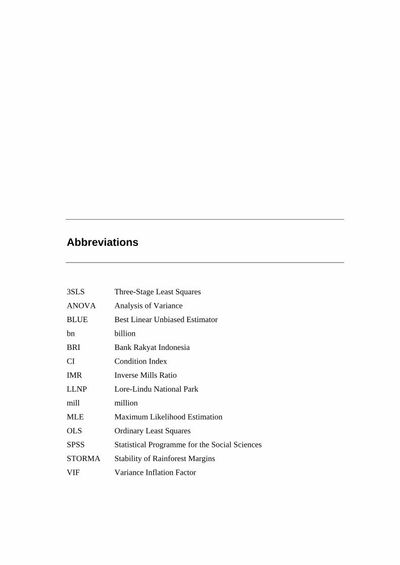
Abbreviations
3SLS Three-Stage Least Squares
ANOVA Analysis of Variance
BLUE Best Linear Unbiased Estimator
bn billion
BRI Bank Rakyat Indonesia
CI Condition Index
IMR Inverse Mills Ratio
LLNP Lore-Lindu National Park
mill million
MLE Maximum Likelihood Estimation
OLS Ordinary Least Squares
SPSS Statistical Programme for the Social Sciences
STORMA Stability of Rainforest Margins
VIF Variance Inflation Factor
Chapter 1
1 Introduction
1.1 Background
The World Bank (1999) estimates that more than 70% of the world’s 1.8 bil-
lion (bn) poor live in rural areas, most of them in developing countries. Therefore,
reducing rural poverty has been on the agenda of international development agencies
as well as governmental and non-governmental organisations for a long time. Since
the 1980s a common approach was through integrated rural development focused on
the agricultural sector. The core instrument was the promotion of Green Revolution
technologies aiming to increase productivity. Due to market failures for smallholders
the state had to distribute and often subsidise the delivery of new technologies, for
example chemical fertiliser and pesticides. The integrated rural development ap-
proach had only limited success and often turned out to be not sustainable (de Janvry
et al., 2002).
Chapter 1: Introduction
2
Succeeding rural development approaches share the distinct feature of taking
a more holistic view on rural households. Among rural households there is a great
degree of heterogeneity in asset position and in income generating activities. Rural
households are engaged in a wide variety of activities: they cultivate crops on their
fields, work as wage labourers on other farms, or operate a small shop. A literature
review on studies concerning the rural non-farm economy by Reardon et al. (1998)
reports a non-farm income share of 42% for Africa, 40% for Latin America and 32%
for Asia. For Indonesia they state that about 35% of rural incomes stem from non-
agricultural activities indicating their importance. However, the figure is not based
on nation-wide data. It is derived from three different studies based on data from
1977, 1983, and 1987 from different regions in Indonesia.
Since the review many studies dealt with the rural non-agricultural sector but
their focus was mainly on Africa and Latin America. Despite its importance indi-
cated by the review there is still little known about non-agricultural activities and on
the role they play in the income generating strategies of rural households in Indone-
sia.
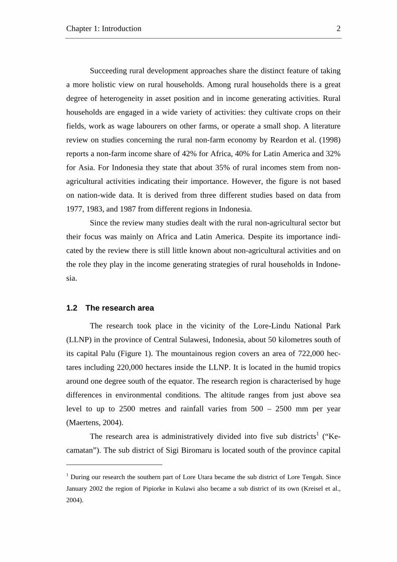
1.2 The research area
The research took place in the vicinity of the Lore-Lindu National Park
(LLNP) in the province of Central Sulawesi, Indonesia, about 50 kilometres south of
its capital Palu (Figure 1). The mountainous region covers an area of 722,000 hec-
tares including 220,000 hectares inside the LLNP. It is located in the humid tropics
around one degree south of the equator. The research region is characterised by huge
differences in environmental conditions. The altitude ranges from just above sea
level to up to 2500 metres and rainfall varies from 500 – 2500 mm per year
(Maertens, 2004).
The research area is administratively divided into five sub districts1 (“Ke-
camatan”). The sub district of Sigi Biromaru is located south of the province capital
1 During our research the southern part of Lore Utara became the sub district of Lore Tengah. Since
January 2002 the region of Pipiorke in Kulawi also became a sub district of its own (Kreisel et al.,
2004).
Chapter 1: Introduction
3
Palu and borders the national park in the south. The sub districts of Palolo and Lore
Utara stretch along the eastern side of the LLNP and the sub district of Kulawi on the
western side. The sub district of Lore Selatan is located south of the national park
(Figure 1).
Figure 1: The research area
Chapter 1: Introduction
4
1.3 Problem analysis
The province of Central Sulawesi is one of the poorest provinces in Indonesia
(Suryahadi and Sumarto, 2001). Based on household survey data, 28% of the house-
holds were classified as poor and more than 42% of the households as vulnerable.
Only six provinces had a higher share of vulnerable households than Central Su-
lawesi. There was a strong increase of 23% in that group compared to figures from
1996. This is the second highest increase of all provinces of Indonesia. Estimates
based on household data are not available for the region surrounding the Lore-Lindu
National Park, but a study based on Rapid Rural Appraisals at the village level re-
ported a mean income of IDR 597,300 in 1997, which is more than 50% below the
official poverty line of IDR 1,165,750 per household. Based on the same figures,
97% of the villages were classified as below the official poverty line (ANZDEC,
1997).
The area is also characterised by an increase in population by 2.4% per year
over the last twenty years, of which 21% is due to immigration (Maertens, 2003).
These people were and are attracted by the income opportunities in coffee and par-
ticularly in cocoa cultivation. During the past two decades the area planted with co-
coa increased from almost zero to 18,000 hectares being a major source of deforesta-
tion often located inside the LLNP (Maertens, 2003). This ongoing encroachment
threatens the integrity of the park, which hosts some of the world’s most unique plant
and animal species. It is home to important populations of endemic bird species, like
the Maleo-bird, and mammals like the Dian’s tarsier, the Anoa or the Babirussa
(Waltert et al., 2003).
Therefore, alternative income sources for rural households are needed which
are able to reduce poverty and the pressure on the national park. A good understand-
ing of the determinants of activity participation as well of the income derived from
these activities is essential for the design of policies promoting alternative income
strategies.
Chapter 1: Introduction
5
1.4 Objectives and research topics
The study aims to identify and analyse the determinants of income generating
activities of rural households in the vicinity of the Lore-Lindu National Park. It helps
to identify factors, which are essentially for the design of policies and programmes
aiming to promote rural development. It is part of project A4 “Economic analysis of
land use systems of rural households” of the Collaborative Research Centre “Stabil-
ity of Rainforest Margins” (STORMA).
The analysis of income generating activities is divided into a descriptive
analysis and into a causal analysis. The descriptive analysis addresses the question
“what” (research questions 1 and 2), whereas the causal analysis seeks to answers the
question “why” (research question 3 until 6). Specifically the following research
questions will be addressed:
1. In which income activities are rural households engaged?
2. Do poor differ from less-poor households in their activities?
3. Which factors influence total household income?
4. Which factors influence the participation in different activities?
5. Which factors influence the income gained from different activities?
6. Which factors influence income diversification?
7. Which policy conclusions can be drawn from the results with respect to
poverty alleviation, deforestation and rural development?
1.5 Outline
Chapter 2 reviews the theoretical and empirical literature on determinants of
income generating activities of rural households. It establishes the conceptual
framework, which is the foundation of the empirical analysis. It begins with a de-
scription of two conceptual approaches, the livelihood and the assets-activities-
Chapter 1: Introduction
6
income approach, which link assets with activity choice and incomes. Then, the con-
ceptual framework is described guiding the further analysis. It stylises the influence
of various socio-economic factors on the activity choice of rural households. The
chapter continuous with a definition of the key terms of this study: assets, activities,
and incomes. The third section reviews the empirical evidence of factors influencing
income generating activities and hypothesises their outcome for our analysis. The
chapter ends with the introduction of a mathematical model of activity choice and
incomes yielding the total income and activity income equations on which the econo-
metric models are based.
Chapter 3 describes the methodology used for the analysis throughout this
work. We present the sampling frame and describe the selection of households. As
empirical studies crucially depend on the data quality, the data collection process as
well as the entering and cleaning of the data are described in detail. We continue
with a description of the measurement of the dependent as well as the independent
variables used in the analysis. Then, the use of sampling weights and the methods
applied to measure statistical inferences are introduced. Chapter 3 ends with the
presentation of the methodology used in the causal analysis. It describes the different
econometric models applied to analyse the influencing factors on total households
income, participation, activity incomes, and income diversity.
Chapter 4 presents the results of the descriptive analysis of income and activi-
ties rural households are engaged in. The analysis follows the differentiation of ac-
tivities introduced in the previous chapter according to sectors and functions. After
illustrating the composition of the total household income over all households it is
shown how this mixture changes according to different socio-economic groups.
Then, the different activities are explored in detail with special emphasis on regional
differences. After evaluating income shares and the degree of income specialisation
the final section looks at the distribution of income. We derive a Lorenz curve to
show graphically the income distribution and calculate the Gini coefficient.
The socio-economic factors influencing activity choice and incomes intro-
duced in the conceptual framework are described in Chapter 5. Emphasis is placed
Chapter 1: Introduction
7
on the variables, which are included in the econometric models in the next chapter.
In the first section the possession of physical capital and its differences between re-
gions is analysed. Then, the demographic structure of rural households and the edu-
cational background of its members are described. The third section shows the access
to social capital, the pattern of migration and the ethnic composition. After evaluat-
ing the participation in financial markets the last section, Chapter 5 briefly describes
the access to road infrastructure.
Chapter 6 presents the results of the econometric models used in this thesis.
The influence of internal and external factors as described in the conceptual frame-
work on total household income, on participation in income activities as well as on
activity incomes is analysed. In the later analysis we consider endogeneity as well as
simultaneity of activity choice. The chapter ends with an evaluation of the influence
of internal and external factors on income diversification.
Chapter 7 summarise the major results of the descriptive as well as the econo-
metric analysis in relation to the research questions presented in Chapter 1.
Chapter 2
2 Conceptual framework
This chapter reviews the theoretical and empirical literature on determinants
of income generating activities of rural households. It establishes the conceptual
framework, which is the foundation of the empirical analysis.
The chapter starts with the discussion of two conceptual approaches linking
assets with activity choice and incomes. Then, the conceptual framework is de-
scribed, which guides the further analysis. Furthermore, this section explores differ-
ent definitions and classifications of assets. The definition of income and its classifi-
cation is presented in the second section. The third section reviews the empirical evi-
dence of determinants of income generating activities and hypothesises their influ-
ence concerning our analysis. The chapter ends with the introduction of a mathemati-
cal model of activity choice and incomes in the last section. It yields the total income
and activity income equations on which the econometric models are based.
Chapter 2: Conceptual framework
9
2.1 Conceptual approaches linking assets with activity choice and incomes
In recent years two approaches emerged in the literature linking income and
activities: the livelihood approach and the assets-activities-incomes approach.
There exists some variation in the definition of a livelihood in the literature.
An early definition is in Chambers and Conway (1992, p.7). To their understanding
livelihood “comprises the capabilities, assets (stores, resources, claims, and access)
and activities required for a means of living”. More recently, Ellis (2000, p.10) de-
fines a livelihood as consisting of “[…] the assets (natural, physical, human, financial
and social capital), the activities, and the access to these (mediated by institutions
and social relations) that together determine the living gained by the individual or
household”. As livelihood and income are not synonymous, they are nevertheless
inseparably connected, because income “at a given point in time is the most direct
and measurable outcome of the livelihood process” (Ellis, 2000, p.10). The liveli-
hood approach emphasises the role of the household’s resources as determinants of
activities and highlights the link between assets, activities and incomes. Moreover, it
stresses the multiplicity of activities rural households are engaged in. A review of
empirical studies concerning rural non-farm incomes by Reardon et al. (1998) shows
their importance for rural households. On average, non-farm incomes contribute 29%
of the total income of rural households in South Asia indicating that a rural house-
hold is not necessarily equivalent to a farm household.
Barrett and Reardon (2000) developed another approach linking assets, activi-
ties and incomes. Having a production function in mind, assets correspond to the
factors of production and incomes to the outputs of production. Activities are the ex
ante production flows of asset services. In contrast to the livelihood approach they
highlight the role of prices in the income generating process. They point out that
“[…] it is crucial to note that the goods and services produced by activities need to
be valued by prices, formed by markets at meso and macro levels, in order to be the
measured outcomes called incomes” (Barrett and Reardon, 2000, p.27).
Chapter 2: Conceptual framework
10
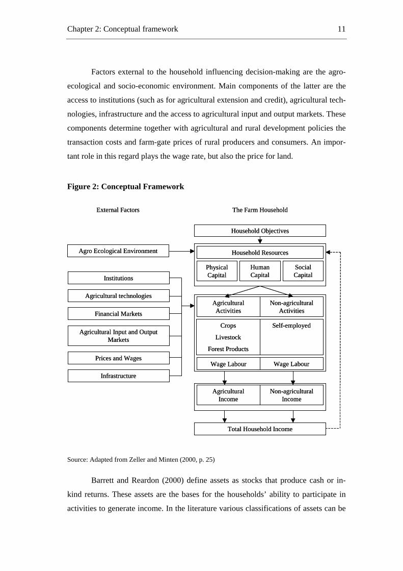
The conceptual framework used in this work builds on the features of these
two approaches linking assets, activities, and incomes. However, more emphasis is
given to factors mediating the use of assets. A similar framework has been used by
Zeller and Minten (2000) to evaluate the consequences of market liberalisation on
the income of rural households.
The household is assumed to maximise its utility which is a function of the
consumption of goods and leisure. It is subject to various constraints, such as a cash
constraint. According to its objective, the household allocates its resources to activi-
ties subject to factors which are external to the household (see Figure 2). These ac-
tivities generate outcomes which will meet the objectives. The activities as well as
the income generated have an effect on the stock of resources available to the house-
hold in the future2. The total household income is the aggregate measure of the out-
come of all the activities the household is engaged in. Determinants of the production
decision which are external to the household, are illustrated on the left hand side of
the conceptual framework. They condition, or as Ellis (2000) calls it, mediate the use
of the household’s resources. The household’s assets are shown on the right hand
side, which also stylises the decision making process of the household.
The household is taken as a single decision-making body. Processes by which
resources are allocated among household members, the so-called intra household
resource allocation, are not taken into account due to limitations in time and budget
for data collection. This implies that consequences of policies can only be modelled
for the household as a whole and not for its individual members3.
2 Such inter-temporal resource allocations are not the subject of this study and hence a broken line
illustrates this relationship. Inter-temporal linkages are investigated in project A3 of STORMA. 3 For a more detailed discussion of the problem of intra household resource allocation see Haddad et
al. (1997).
Chapter 2: Conceptual framework
11
Factors external to the household influencing decision-making are the agro-
ecological and socio-economic environment. Main components of the latter are the
access to institutions (such as for agricultural extension and credit), agricultural tech-
nologies, infrastructure and the access to agricultural input and output markets. These
components determine together with agricultural and rural development policies the
transaction costs and farm-gate prices of rural producers and consumers. An impor-
tant role in this regard plays the wage rate, but also the price for land.
Figure 2: Conceptual Framework
Household Resources
Physical Capital
Social Capital
Human Capital
AgriculturalActivities
Non-agricultural Activities
Total Household Income
Agro Ecological Environment
Institutions
Financial Markets
Agricultural Input and OutputMarkets
Prices and Wages
Infrastructure
Household Objectives
AgriculturalIncome
Non-agricultural Income
Crops
Livestock
Forest Products
Self-employed
Wage Labour Wage Labour
The Farm HouseholdExternal Factors
Agricultural technologies
Source: Adapted from Zeller and Minten (2000, p. 25)
Barrett and Reardon (2000) define assets as stocks that produce cash or in-
kind returns. These assets are the bases for the households’ ability to participate in
activities to generate income. In the literature various classifications of assets can be
Chapter 2: Conceptual framework
12
found. For example, Reardon and Vosti (1995) differentiate natural, human, on-farm
physical capital, off-farm physical capital, and community owned resources. Barrett
and Reardon (2000) propose to distinguish productive and non-productive assets.
Productive assets are inputs used in the production process and therefore generate
income indirectly via the activities. In contrast, non-productive assets generate in-
come directly through transfers or capital gains. Furthermore, they propose a distinc-
tion based on ownership. Ellis (2000) distinguishes natural, physical, human, social,
and financial capital. He claims that his categorisation can solve the anomalies be-
tween the different researchers, but without giving clear definitions to differentiate
them.
In our analysis we follow the asset classification proposed by Vosti and
Reardon (1995) but without a spatial differentiation of physical capital. Additionally
we differentiate explicitly the household member’s access to social networks and
institutions. Recent empirical studies highlight the important influence of social capi-
tal on household welfare and poverty (Narayan and Pritchett, 1997, Grootaert, 1999,
Collier, 1998). Thus, the household’s resources are classified as physical capital
(land, livestock, and other assets owned), human capital (labour, education, gender
and age), and social capital (access to social networks and institutions).
2.2 Definition of income and its classification
As income is defined as the output of activities it measures both cash and in-
kind contributions. All the goods and services produced in activities are valued at
market producer prices regardless of their use. So, all own-farm products are valued
at the same price as if they were sold (Ellis, 2000).
In the literature there has been a wide range of different systems in classifying
sources of income. Terms like off-farm and non-farm income are used in an at first
glance synonymous way, but with slightly different definitions. Ellis (2000) for ex-
ample defines off-farm income as income originating from wage labour on other
farms whereas Barrett et al. (2001) refer to off-farm income as all activities away
from the farmer’s own property. We follow the classification proposed by Barrett et
Chapter 2: Conceptual framework
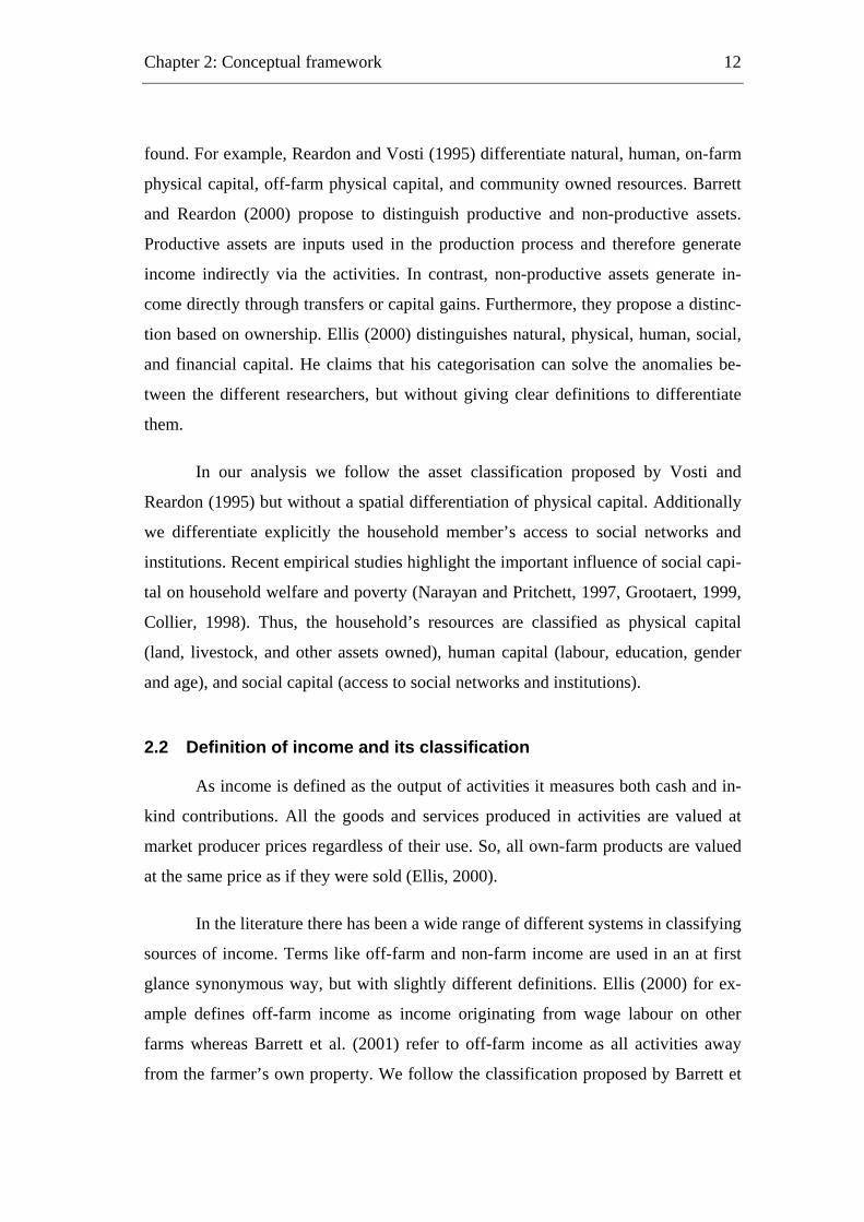
13
al. (2001) according to sectors (agriculture and non-agriculture) and functions (wage
and self-employment). The third criteria used, spatial classification, is not distin-
guished here because there is not a single household in the sample where income
from migrated household members is relevant. All income derived is therefore classi-
fied as local. Figure 3 illustrates the concept and the classification of the different
income sources.
Figure 3: Classification of activities according to functions and sectors
Function Agriculture Non-agricultureSelf-employment Annual crops Enterprises
Perennial crops RentsLivestockForest products/Fishing
Wage employment Agricultural wage labour Non-agricultural wage labourSource: Adapted from Barrett et al. (2001)
Sector
In the analysis we distinguish the income activities mentioned in Figure 3, but
aggregate income from enterprises and rents to non-agricultural self-employed in-
come. This differentiation also allows a detailed analysis of the non-agricultural sec-
tor, because it might represent an income opportunity for rural poor without leading
to further encroachments. We further differentiate agricultural self-employment into
four different activities, because the analysis of perennial crop production is particu-
larly important as the encroachment into the national park is mainly driven by cocoa
(Maertens, 2003). Moreover, the collection of forest products in the LLNP also de-
serves special attention.
2.3 Review of empirical evidence on determinants influencing income generating activities
As depicted in Figure 2 the approach applied focuses on the access to the dif-
ferent types of assets which is conditioned by external factors, like institutions and
Chapter 2: Conceptual framework
14
infrastructure. In this section we review the empirical evidence on determinants in-
fluencing activity choice and activity income.
Why do households diversify their activities and increase for example their
income from activities outside agriculture? They change because returns to their as-
sets endowed in agricultural production decrease in relation to the returns from using
them in activities outside agriculture. This implies that the choice of activities highly
depends on access to the different types of assets (Winters et al., 2002 and Barrett et
al., 2001) and also explains why not all households have the same opportunities to
participate in non-agricultural activities. Poorer households tend to have less access
to non-farm activities than households that are better off. Moreover, there is a strong
link between non-farm income share and total household income (Reardon et al.,
1998). In the econometric model we will explore this relationship by including the
value of other assets owned as a welfare indicator. These other physical assets are
mainly unrelated to agricultural production. The area of land and the livestock units
owned are also included as explanatory variables in the regression models to account
for the influence of physical capital related to agriculture on activity choice. In the
activity choice and income models we distinguish the possession of rainfed and irri-
gated land to investigate the influence of paddy rice production on the production of
perennial crops and furthermore on the encroachment into the LLNP.
In a literature review, Barrett et al. (2001) find a strong positive relation be-
tween education and non-farm incomes in almost all of the papers reviewed. Never-
theless, when also considering the agricultural sector than the results are mixed.
Jolliffe (1998) reports for Ghana that schooling has a negative influence on income
from agricultural self-employment, whereas it has a positive impact on total and off-
farm income4. In Mexico, Taylor and Yunez-Naude (2000) find high returns from
schooling in wage labour, whereas the returns in the production of staples are low
and not significant. These results reveal the importance of activity differentiation.
Moreover, they show the need for a clear definition of the income activities to make
4 Jolliffe (1998) refers to off-farm income as the aggregate of wage income and income from self-
employment outside agriculture.
Chapter 2: Conceptual framework
15
the results more easily comparable. In this study we include the years in school of the
head of the household as a proxy for education. Besides education, we also control
for the influence of ethnicity on activity choice and income.
Other than human capital, access to social capital can also play an important
role. Narayan and Pritchett (1997) demonstrate with an econometric model for Tan-
zania, that social capital has a higher influence on household income than human or
physical capital. Grootaert (1999) highlights the important influence of social capital
on welfare and poverty in Indonesia. In terms of activity choice social capital can
foster the ability to participate in many different income activities. To test whether
the density of a social network has any influence on activity choice and incomes we
include a social capital index, measuring the access and the influence of household
members in formal institutions. Moreover, we also include a variable measuring the
ethnicity of the head of the household since this can influence the access to informal
social networks.
Less-poor households do not only own more productive assets, but also have
better access to markets, especially to financial markets. Limited access to credit can
either “push” poor households into wage labour activities to earn cash (Reardon et
al., 1998) or it further restricts their ability to invest in non-agricultural activities.
Poor households are not able to adjust their capital stock to the different needs in
activities outside agriculture. Households which have access to credit are able to par-
ticipate in credit markets, but they may choose not to do so or may borrow less than
they could (Diagne et al., 2000). Due to difficulties in measuring access to credit, we
measured the participation in formal credit markets by using a dummy variable
which is “one” when the household received a formal credit in the last five years and
“zero” otherwise.
Studies by Canagarajah et al. (2001) in Tanzania and Smith et al. (2001) in
Uganda show that better physical access to markets increases non-farm earnings.
Thus, we include the distance from the homestead to the next tarmac road in our
econometric models. Nevertheless, it is difficult to distinguish the effect of the dis-
tance to roads from other spatially fixed effects. To control for these effects we in-
Chapter 2: Conceptual framework
16
clude location dummies, which are equivalent to the four sub districts in our research
area.
In the context of income diversification various studies highlight the impor-
tance of risk. Studies by de Janvry et al. (1991) and Kinsey et al. (1998) indicate that
income diversification is positively correlated with an increased ability to cope with
shocks. Diversification is a way rural households insure themselves against the oc-
currence of such shocks. Therefore we included a variable in the model on income
diversification measuring the number of harvests failed in the last 10 years.
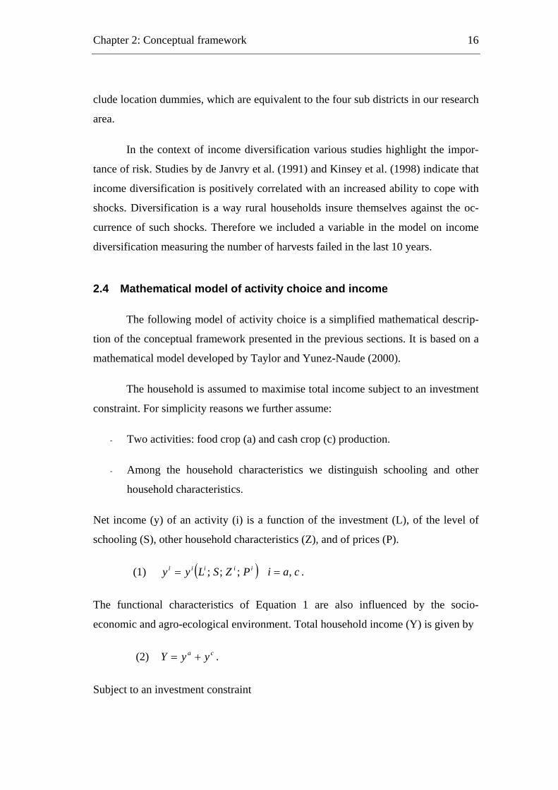
2.4 Mathematical model of activity choice and income
The following model of activity choice is a simplified mathematical descrip-
tion of the conceptual framework presented in the previous sections. It is based on a
mathematical model developed by Taylor and Yunez-Naude (2000).
The household is assumed to maximise total income subject to an investment
constraint. For simplicity reasons we further assume:
- Two activities: food crop (a) and cash crop (c) production.
- Among the household characteristics we distinguish schooling and other
household characteristics.
Net income (y) of an activity (i) is a function of the investment (L), of the level of
schooling (S), other household characteristics (Z), and of prices (P).
(1) ( ) caiPZSLyy iiiii ,;;; == .
The functional characteristics of Equation 1 are also influenced by the socio-
economic and agro-ecological environment. Total household income (Y) is given by
(2) . ca yyY +=
Subject to an investment constraint
Chapter 2: Conceptual framework
17
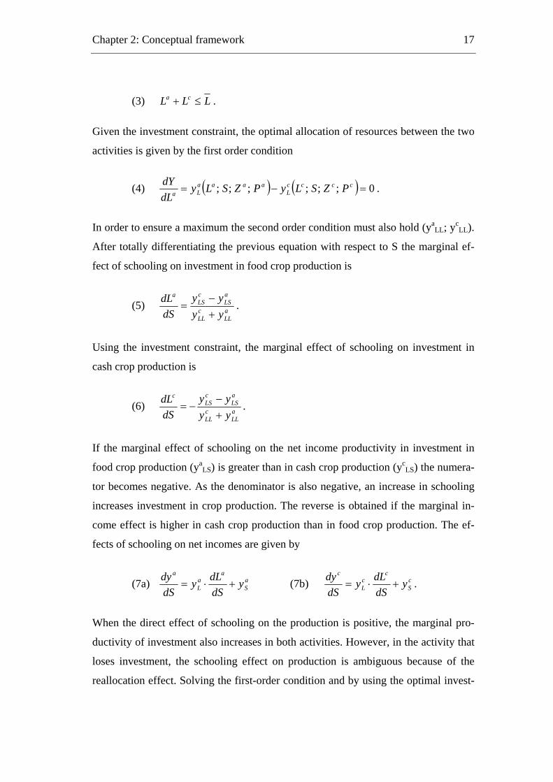
(3) LLL ca ≤+ .
Given the investment constraint, the optimal allocation of resources between the two
activities is given by the first order condition
(4) ( ) ( ) 0;;;;;; =−= ccccL
aaaaLa PZSLyPZSLy
dLdY .
In order to ensure a maximum the second order condition must also hold (yaLL; yc
LL).
After totally differentiating the previous equation with respect to S the marginal ef-
fect of schooling on investment in food crop production is
(5) aLL
cLL
aLS
cLS
a
yyyy
dSdL
+−
= .
Using the investment constraint, the marginal effect of schooling on investment in
cash crop production is
(6) aLL
cLL
aLS
cLS
c
yyyy
dSdL
+−
−= .
If the marginal effect of schooling on the net income productivity in investment in
food crop production (yaLS) is greater than in cash crop production (yc
LS) the numera-
tor becomes negative. As the denominator is also negative, an increase in schooling
increases investment in crop production. The reverse is obtained if the marginal in-
come effect is higher in cash crop production than in food crop production. The ef-
fects of schooling on net incomes are given by
(7a) aS
aaL
a
ydSdLy
dSdy
+⋅= (7b) cS
ccL
c
ydSdLy
dSdy
+⋅= .
When the direct effect of schooling on the production is positive, the marginal pro-
ductivity of investment also increases in both activities. However, in the activity that
loses investment, the schooling effect on production is ambiguous because of the
reallocation effect. Solving the first-order condition and by using the optimal invest-
Chapter 2: Conceptual framework
18
ment in the activity income equation obtains the reduced form activity income equa-
tions
(8) ( ) caiPZSyy iiii ,;;; ==
The activity income equations are linked by the reallocation effect. Thus, income
from one activity depends on the variables affecting both activities. Total income is
given by
(9) ( ) caiPZSyYi
iii ,;;; == ∑
The econometric modelling of activity choice and incomes in the following chapter
is based on the last two equations.
The mathematical model presented is a simplification of the conceptual
framework, as it explicitly shows one form of capital, human capital, only. Other
forms of capital are modelled implicitly through the investment constraint L. An ex-
tension of the model to explicitly take into account all four types of capital men-
tioned in the conceptual framework is possible. It is not shown here because the
mathematical formulation becomes very complex. Furthermore, the basic arguments
stay the same only that the marginal rates of return to different types of capital have
to be equal in the optimal solution. Another possible extension concerns the objective
function which can be extended to assume utility maximisation under a consumption
and a leisure constraint. Moreover, the inclusion of a food subsistence constraint re-
flects a situation where the access to food markets is limited. Households are forced
to cultivate more food crops for home consumption compared to households with
better access to markets for basic staples.
2.5 Summary
This chapter reviewed the theoretical and empirical literature on determinants
of income generating activities of rural households. The conceptual framework,
which is the foundation of the empirical analysis was established. The livelihood
Chapter 2: Conceptual framework
19
approach and the assets-activities-income approach were discussed as they link as-
sets with activity choice and incomes. The conceptual framework was then described
guiding the further analysis. It stylises the influence of various socio-economic fac-
tors on the activity choice of rural households. In the literature various definitions of
assets, activities, and incomes exist. We reviewed the literature concerning these key
terms and thoroughly defined them for the purposes of our study. Assets are distin-
guished into physical, human and social capital. Activities and incomes are classified
according to functions and sectors. In the following analysis we will distinguish agri-
cultural self-employment, agricultural wage labour, non-agricultural self-
employment, and non-agricultural wage labour. Because of its importance the cate-
gory agricultural self-employment is further differentiated into annual and perennial
crop production, livestock production and the sale of forest products. Based on a lit-
erature review the influence of various factors on income generating activities was
hypothesised. Finally, a mathematical model of activity choice and incomes was in-
troduced which yields the total income and activity income equations for the econo-
metric models.
The review of the theoretical and empirical literature leads to the formulation
of hypotheses and to the design of a conceptual framework, which was then de-
scribed in a mathematical model. The whole conceptual framework was the founda-
tion for the data collection process. The next chapter describes how the necessary
data was collected, processed, and analysed.
Chapter 3
3 Methodology
This chapter presents the methodology used to answer the research questions
of this study. After presenting the sampling frame and the selection of households,
the data collection, the entering and the cleaning of the data is described. The third
section in this chapter presents the measurement of the dependent as well as the in-
dependent variables used in the econometric analysis. The following section deals
with the methodology used in the descriptive analysis. It describes the use of sam-
pling weights and the methods applied to measure statistical inferences. The last sec-
tion presents the methodology used in the causal analysis. It describes the different
econometric models applied to analyse the influencing factors on total households
income, participation, activity incomes, and income diversity.
Chapter 3: Methodology
21
3.1 Sampling frame and selection of households
As this study is part of Project A4 of the Collaborative Research Centre
STORMA, we used the common sampling frame agreed upon by all participating
projects. The procedures used for the selection of villages and households are de-
scribed in detail in Zeller et al. (2002a). This section describes the main stages in the
selection process and highlights some important methodological aspects.
The population for the study are all households living in the 117 villages of
the research area. The observation unit is the rural household. A multi-stage sam-
pling design was used because a sampling frame at the household level did not al-
ready exist for the research area and the costs of construction would have been high.
As a list of villages and additional information for 115 villages is contained in
ANZDEC (1997) villages were used as first stage sampling units. Beyond the selec-
tion procedure this arrangement also has the advantage of being more cost-effective
for the survey. The enumerators do not have to visit households living widely dis-
persed from each other. They can work in survey teams travelling together from vil-
lage to village. Working in teams also has the advantage of strengthening the moral
of the enumerators (Deaton, 1997, Poate and Daply, 1993). As the survey becomes
more cost-effective, the supervision is also less costly and easier to organise.
Before selecting the villages they were divided into mutually exclusive sub-
populations, the so-called strata, which were then sampled independently. The main
reason for choosing this procedure was to ensure catching the large differences in
agro-ecological and socio-economic conditions affecting land-use. It was hypothe-
sised that the following three criteria have a strong influence on the practices of land
cultivation in the research area (Zeller et al., 2002a):
- Proximity of the village to the park (two subgroups)
- Population density (two subgroups)
- Ethnic composition (three subgroups)

Chapter 3: Methodology
22
The 115 villages were divided into 12 strata according to these three selection
criteria. After inspection of the data it turned out that one stratum was empty and
another one contained only one village. This village was grouped into another strata
and ten strata remained. In three subsequent steps 80, 20 and 12 villages have been
selected out of the 10 strata. In the latter sub sample it was assured that at least one
village out of each strata was chosen (Zeller et al., 2002a). During a field visit at the
beginning of 2001, it was recognised that the village of Wanga was grouped into a
wrong strata due to an error in the report of ANZDEC (1997). After regrouping this
village, another strata became empty and 9 strata remained.
The precision of the statistical estimates depends on the procedures used in
the sampling frame. While stratification usually increases the precision of the sam-
pling estimates, clustering reduces it. Within a cluster households are usually more
similar to each other than to households in other clusters, especially when the clus-
ters represent different localities. Due to environmental and climatic effects land-use
might be more similar within a village than between villages (Deaton, 1997, Poate
and Daply, 1993). The effect of clustering and stratification could not be incorpo-
rated into the analysis because of software limitations5.
In a second stage, 301 households were randomly selected out of the 12 vil-
lages. The number of selected households in every village was chosen according to
the share in the overall population of the strata, but adjustments have been made ac-
cording to village size and the proximity to the National Park. In small villages a
higher number of households have been selected due to cost and logistic considera-
tions. In villages close to the LLNP more households have been selected, as
STORMA is particularly interested in households and their plots close to the national
5 At the time of writing, Stata 8 is the only software package which is able to take the effects of clus-
tering and stratification into account. Unfortunately, it requires that each stratum contains more than
one village, which is not the case in our study.
Chapter 3: Methodology
23
park. In every village, a list containing all households in the village6 was compiled.
In all villages administrative records exist, but there accuracy varied greatly. There-
fore, existing records have been updated with the help of the villagers. To ensure that
households from the entire list can be drawn, the step size was calculated by dividing
the number of households in the list by the sample size. The first household to be
chosen was determined by randomly selecting a number between one and the value
of the step size (Zeller et al 2002a).
The number of households chosen in the different strata has not been propor-
tional to the strata’s share in total population. In order to extrapolate results from the
sample to the population, the descriptive analysis as well as the econometric analysis
has to use sampling weights. The sampling weights W are calculated for strata i as
(10) ⎟⎠⎞
⎜⎝⎛
⎟⎠⎞
⎜⎝⎛=
Ss
Nn
W iii / ,
where ni is the number of households in strata i and si is the number of households
being sampled out of strata i. N refers to the total number of households in the re-
search area and S to the total number of households being sampled. Table 1 gives an
overview of the randomly selected villages for STORMA and their corresponding
sampling weights.
6 In Maranata, a large village in the district of Sigi-Biromaru, a random sub-sample of the districts of
the village (dusun) were chosen to reduce survey costs. Only households in dusun number 1, 2, and 5
have been selected.
Chapter 3: Methodology
24
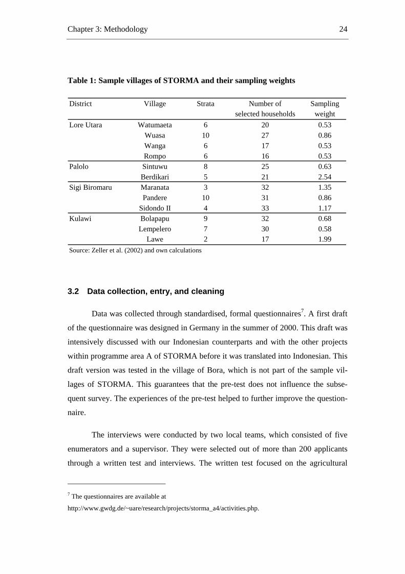
Table 1: Sample villages of STORMA and their sampling weights
District Village Strata Number of Samplingselected households weight
Lore Utara Watumaeta 6 20 0.53Wuasa 10 27 0.86Wanga 6 17 0.53Rompo 6 16 0.53
Palolo Sintuwu 8 25 0.63Berdikari 5 21 2.54
Sigi Biromaru Maranata 3 32 1.35Pandere 10 31 0.86
Sidondo II 4 33 1.17Kulawi Bolapapu 9 32 0.68
Lempelero 7 30 0.58Lawe 2 17 1.99
Source: Zeller et al. (2002) and own calculations
3.2 Data collection, entry, and cleaning
Data was collected through standardised, formal questionnaires7. A first draft
of the questionnaire was designed in Germany in the summer of 2000. This draft was
intensively discussed with our Indonesian counterparts and with the other projects
within programme area A of STORMA before it was translated into Indonesian. This
draft version was tested in the village of Bora, which is not part of the sample vil-
lages of STORMA. This guarantees that the pre-test does not influence the subse-
quent survey. The experiences of the pre-test helped to further improve the question-
naire.
The interviews were conducted by two local teams, which consisted of five
enumerators and a supervisor. They were selected out of more than 200 applicants
through a written test and interviews. The written test focused on the agricultural
7 The questionnaires are available at
http://www.gwdg.de/~uare/research/projects/storma_a4/activities.php.

Chapter 3: Methodology
25
knowledge and the arithmetic skills of the candidate, whereas the interview tried to
assess personality and character.
The selected candidates were mixed concerning religion and ethnicity. All of
them had completed at least high school and some had even finished BSc.-Study at
UNTAD University. Out of the group of candidates we selected two supervisors who
were responsible for supervision and organisation of the field work. They also repre-
sented the group in the villages.
Prior to the survey the enumerators were extensively trained in the classroom
and in the field. In the classroom, the first part of the training, the enumerators were
familiarised with the survey. The objectives of the survey were explained as well as
the relevance to local and national development. Each question of the questionnaire
was discussed in detail regarding its reason, measurement, concepts, coverage, and
the reference period. Finally, the interview situation was trained using role-playing.
The field training again took place in the village of Bora. During the training the
enumerators went in teams of two to the respondents. The interviews were analysed
by the senior field staff. The experiences of the enumerators with the respondents
and the questionnaire were discussed, which helped to finalise the questionnaire.
The teams were guided by senior field staff consisting of members of the
STORMA research project. The first survey took place from December 2000 until
March 2001. The data was entered twice by different enumerators at UNTAD Uni-
versity in Palu. The two versions were compared using SPSS Data Entry, which re-
cords differences between the versions. In case of inconsistencies, the entry was
compared with the information in the questionnaire. This procedure minimises data
entry errors. After entering the data was cleaned, which consisted of examining the
data for missing values, wild codes, inconsistencies, and extreme values.
Due to the high amount of information needed within Project A4 of
STORMA, the households were visited twice. In the first survey the focus was on
household composition, land and livestock possession, and the use of inputs and out-
puts. Additionally, all the questions needed to calculate the poverty index have been
Chapter 3: Methodology
26
included. A second visit followed, asking questions about changes in the household
composition and the possession of land and livestock. Once again, the focus was the
use of inputs and outputs on agricultural plots and additional questions on wage la-
bour and business income were included. The same enumerators and supervisors
were employed and the same procedures used for the first survey were applied. The
second survey took place from August until October 2001.
In the first survey, all 301 households which were selected were interviewed.
During the second round of the survey the number of households dropped to 293
because five households moved and three refused to cooperate any longer with
STORMA. We decided not to replace these households, as the sample size was still
sufficient.
Additionally, information was drawn from secondary data, interviews with
experts, and from the results of other sub-programmes. Of special interest was the
work of sub-project A3, which collected data about the regional market and policy
environment in the same twelve villages, where the household survey was conducted.
3.3 Measurement of the dependent variables
3.3.1 Measurement of income
The total household income is the sum of the net income from agricultural
and non-agricultural self-employment and wage labour activities (see Figure 3 in
Chapter 2.2). The net income from an activity is obtained by subtracting the cash
expenses incurred in production from the gross income (Taylor and Turner, 1998).
All data needed to calculate the crop income was collected at the plot level.
To make the recall process easier for the respondents we asked in the case of annual
crops, only for the yield and the input expenditures of the last crop harvested. Data
from both rounds covers about one year of activities. Nevertheless, a possible meas-
urement error occurs due to the possibility of almost three harvests per year on some
plots in the case of paddy rice, maize, and vegetables. In the case of perennial crops,
Chapter 3: Methodology
27
it was not possible to ask only for the last harvest because some crops, like for exam-
ple cacao, are harvested continuously over the year. Therefore, we decided to use a
recall period of one year for perennial crops. The gross income from crop production
was obtained as the sum of all crops produced during the recall period valued at the
market producer price. So all the crops produced were valued at the same price re-
gardless whether they were being sold or consumed at home. If a market producer
price for a specific crop was missing at the household level, the corresponding vil-
lage level price was used. If a village level price was not obtained the next level
prices were used and so on up to the highest level, the overall sample price. To re-
flect the high opportunity costs in marketing their products, the market producer
prices in the village of Lawe was reduced by IDR 500 per kg of output. All of the
products sold were brought to the village of Gimpu by horse, which is about one day
travelling from Lawe. The net income was obtained by subtracting the sum of the
cash expenses for land preparation, seeds, fertiliser, irrigation, pesticides, transport,
and hired labour from the gross income. The labour component consisted of wages
paid in cash and in-kind. We did not consider fixed costs like overhead costs for ma-
chinery, as it is not relevant in the region.
The data needed for calculating the income from livestock production was
gathered at the livestock level. The gross income from livestock production is the
sum of the value sold and the value slaughtered for home consumption between
round one and two. The latter was calculated by multiplying the number of animals
slaughtered times the mean value of the animals of this type owned. Any other ani-
mal products, for example milk, are not relevant in the region. The same applies for
by-products, like manure. A third component of the gross income from animal activi-
ties are inventory increases (Turner and Taylor, 1998). As the inventory changes
from round one to round two turned out to be quite numerous in a fraction of the
households interviewed, the income from livestock would have been extraordinary
high. As this does not reflect reality we decided to drop this gross income compo-
nent. From the gross income the variable costs, which is the value of animals pur-
chased and the value of the animals lost due to death or theft, have been subtracted.
Finally, these figures have been adjusted for a whole year. In the case of poultry, for
Chapter 3: Methodology
28
simplicity reasons gross income was assumed as the mean value of poultry owned
between the two surveys.
The income from fishing is the value of fishes caught. Due to problems in
valuing the forest products gathered for home consumption, forest products income
contains only the value of the products sold in the last twelve months. Wage labour
incomes are the sum of the earnings of the individual household members. Income
from enterprises is the profit of the business minus expenditures for labour and other
inputs. In the research area, various rental arrangements exist for example share ten-
ancy. Despite the different arrangements, in all cases the rent received considers cash
as well as in-kind payments and the value of inputs provided by the owner is de-
ducted.
In the evaluation of the different income activities three different aspects are
analysed: participation, activity incomes, and income shares. Participation measures
whether a household is involved in an activity or not. By definition, the household
participates if the activity income is different from zero. In the case of zero activity
incomes the household does not participate. Activity income refers to the income
from a certain activity measured in IDR. The percentage shares in activity incomes
are calculated by dividing the mean activity incomes by the mean total income.
These shares provide an insight into the importance of certain activities for the re-
gion. They should not be mixed-up with income shares, which is the mean of the
percentage share of the income from an activity in total household income. Income
shares highlight the importance of activities at the household level.
3.3.2 Measuring income diversity
To quantify the degree of diversification out of agriculture we use the share of
non-agricultural income in total household income. As a measure of the overall di-
versity of income we apply the Shannon equitability index. It is derived from the
Shannon index (H), which is usually used to assess the diversity of species (Magur-
ran, 1988). Adapting it for our purposes leads to:
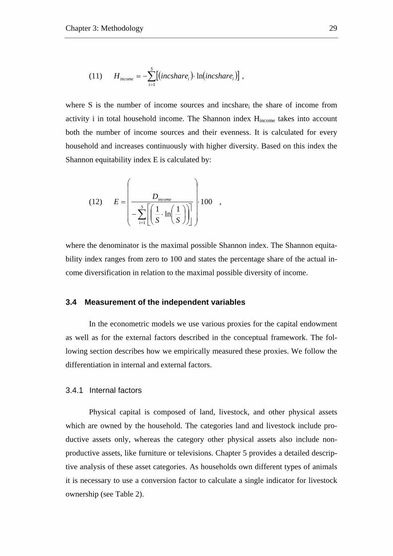
Chapter 3: Methodology
29
(11) ( ) ( )[ ] ,ln1∑=
⋅−=S
iiiincome incshareincshareH
where S is the number of income sources and incsharei the share of income from
activity i in total household income. The Shannon index Hincome takes into account
both the number of income sources and their evenness. It is calculated for every
household and increases continuously with higher diversity. Based on this index the
Shannon equitability index E is calculated by:
(12) ,1001ln1
1
⋅
⎟⎟⎟⎟⎟
⎠
⎞
⎜⎜⎜⎜⎜
⎝
⎛
⎥⎦
⎤⎢⎣
⎡⎟⎟⎠
⎞⎜⎜⎝
⎛⎟⎠⎞
⎜⎝⎛⋅−
=
∑=
S
i
income
SS
DE
where the denominator is the maximal possible Shannon index. The Shannon equita-
bility index ranges from zero to 100 and states the percentage share of the actual in-
come diversification in relation to the maximal possible diversity of income.
3.4 Measurement of the independent variables
In the econometric models we use various proxies for the capital endowment
as well as for the external factors described in the conceptual framework. The fol-
lowing section describes how we empirically measured these proxies. We follow the
differentiation in internal and external factors.
3.4.1 Internal factors
Physical capital is composed of land, livestock, and other physical assets
which are owned by the household. The categories land and livestock include pro-
ductive assets only, whereas the category other physical assets also include non-
productive assets, like furniture or televisions. Chapter 5 provides a detailed descrip-
tive analysis of these asset categories. As households own different types of animals
it is necessary to use a conversion factor to calculate a single indicator for livestock
ownership (see Table 2).
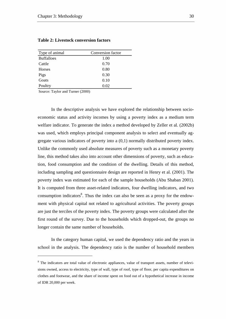
Chapter 3: Methodology
30
Table 2: Livestock conversion factors
Type of animal Conversion factorBuffalloes 1.00Cattle 0.70Horses 0.80Pigs 0.30Goats 0.10Poultry 0.02Source: Taylor and Turner (2000)
In the descriptive analysis we have explored the relationship between socio-
economic status and activity incomes by using a poverty index as a medium term
welfare indicator. To generate the index a method developed by Zeller et al. (2002b)
was used, which employs principal component analysis to select and eventually ag-
gregate various indicators of poverty into a (0,1) normally distributed poverty index.
Unlike the commonly used absolute measures of poverty such as a monetary poverty
line, this method takes also into account other dimensions of poverty, such as educa-
tion, food consumption and the condition of the dwelling. Details of this method,
including sampling and questionnaire design are reported in Henry et al. (2001). The
poverty index was estimated for each of the sample households (Abu Shaban 2001).
It is computed from three asset-related indicators, four dwelling indicators, and two
consumption indicators8. Thus the index can also be seen as a proxy for the endow-
ment with physical capital not related to agricultural activities. The poverty groups
are just the terciles of the poverty index. The poverty groups were calculated after the
first round of the survey. Due to the households which dropped-out, the groups no
longer contain the same number of households.
In the category human capital, we used the dependency ratio and the years in
school in the analysis. The dependency ratio is the number of household members
8 The indicators are total value of electronic appliances, value of transport assets, number of televi-
sions owned, access to electricity, type of wall, type of roof, type of floor, per capita expenditures on
clothes and footwear, and the share of income spent on food out of a hypothetical increase in income
of IDR 20,000 per week.
Chapter 3: Methodology
31
below fifteen and above 60 years old divided by the number of the remaining house-
hold members. The years in school are calculated based on the level of schooling of
the individual household members.
The social capital index of a household was calculated by multiplying the
number of memberships in organisations by the so-called decision making index
(Grootaert, 1999). The number of memberships measures the density of membership
and includes all kinds of groups and the memberships of all household members.
Moreover, the head of the household and the spouse were asked to name up to three
most important associations they were members of. They were asked to evaluate sub-
jectively whether they were “very active”, “somewhat active” or “not very active” in
the decision making process of the group. The response was scaled from 2 (“very
active”) to 0 (“not very active”), respectively, and averaged across the number of
organisations regarded as important by the head of the household and the spouse.
Multiplying by, 50 this figure was re-scaled from 0 to 100 to form the decision mak-
ing index.
3.4.2 External factors
In the questionnaire the households were asked detailed questions about the
different types of credit they received. We assumed that the households access
smaller informal credits more often than bigger informal credits. Therefore, we dif-
ferentiated them into informal credit below IDR 30,000, informal credit between IDR
30,000 and IDR 50,000 and informal credit above IDR 50,000. To reduce the costs
of data collection we referred the first category to the last 8 weeks, whereas for the
other two types of credit the recall period was 8 months. For credit from formal
sources we referred the question to the last five years as we assumed that they are
accessed much less frequently. Due to the differences in the recall period it is not
possible to directly compare formal and informal credits.
The distance to the next tarmac road is used as a proxy for the access to road
infrastructure. Each respondent was asked to estimate how many hours he needs to
get to the next tarmac road on foot.

Chapter 3: Methodology
32
3.5 Methodology used in the descriptive analysis
Besides the minimum and maximum values of variables, the descriptive
analysis also provides means as a measure of central tendency and the standard de-
viation as a measure of the variability. Moreover, we used frequency tabulations and
cross-tabulations. All the results presented are weighed results by applying the sam-
pling weights presented earlier in this chapter. As a characteristic of the computer
package used9 the number of cases presented are also weighed counts. The 293
households interviewed represent the 290 weighed observations reported in the de-
scriptive tables. In contrast to the point estimates, the standard errors of these esti-
mates have not been corrected for sampling effects.
When observing differences in the mean of variables or among groups of a
variable, we do not know whether the difference is a real one or whether it is just by
chance. We have to apply statistical tests to ensure that the observed difference is
statistically significant. To evaluate differences in the mean between two variables
we applied paired t-tests. An example is the difference in the illiteracy rate between
male and female household members.
In the case of comparing the mean of three or more groups of the same vari-
able, Analysis of Variance (ANOVA) was applied. An example is the difference in
participation in agricultural wage labour activities by poverty group. The ANOVA is
based on an F-test which has the following underlying assumptions (Black, 1999):
- Interval or ratio scaled variables
- Each sample observation is randomly drawn from the population
- The sampling distribution of the mean is approximately normal
- The variances of the groups are homogeneous
9 The Statistical Programme for the Social Sciences (SPSS) version 11.0 was used for the descriptive
analysis except for calculating the Gini coefficient.
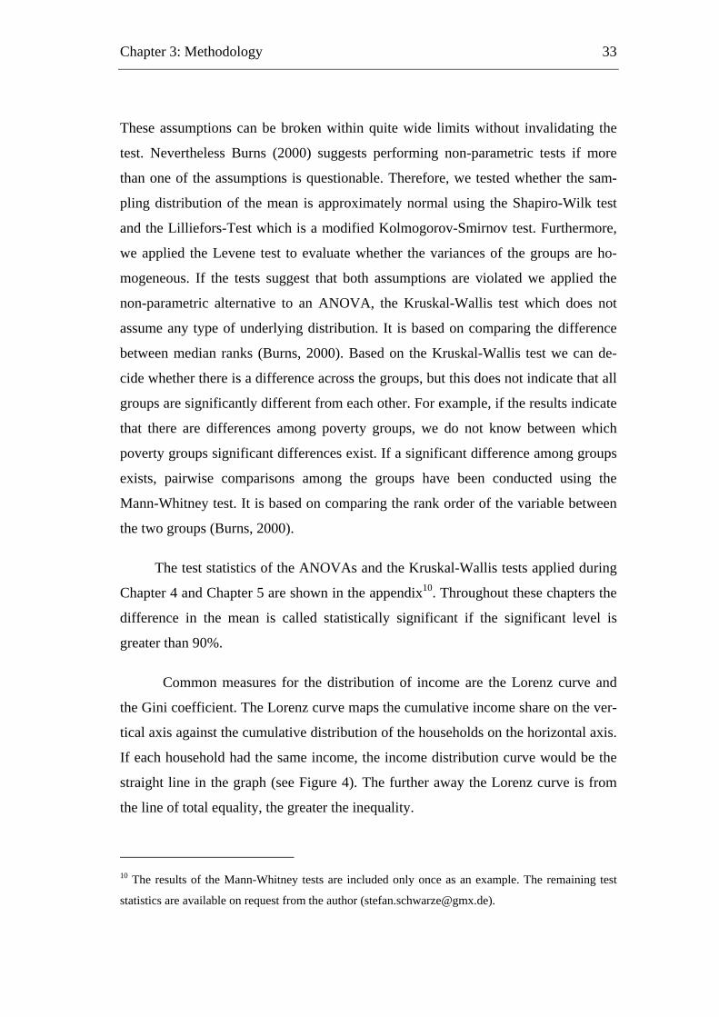
Chapter 3: Methodology
33
These assumptions can be broken within quite wide limits without invalidating the
test. Nevertheless Burns (2000) suggests performing non-parametric tests if more
than one of the assumptions is questionable. Therefore, we tested whether the sam-
pling distribution of the mean is approximately normal using the Shapiro-Wilk test
and the Lilliefors-Test which is a modified Kolmogorov-Smirnov test. Furthermore,
we applied the Levene test to evaluate whether the variances of the groups are ho-
mogeneous. If the tests suggest that both assumptions are violated we applied the
non-parametric alternative to an ANOVA, the Kruskal-Wallis test which does not
assume any type of underlying distribution. It is based on comparing the difference
between median ranks (Burns, 2000). Based on the Kruskal-Wallis test we can de-
cide whether there is a difference across the groups, but this does not indicate that all
groups are significantly different from each other. For example, if the results indicate
that there are differences among poverty groups, we do not know between which
poverty groups significant differences exist. If a significant difference among groups
exists, pairwise comparisons among the groups have been conducted using the
Mann-Whitney test. It is based on comparing the rank order of the variable between
the two groups (Burns, 2000).
The test statistics of the ANOVAs and the Kruskal-Wallis tests applied during
Chapter 4 and Chapter 5 are shown in the appendix10. Throughout these chapters the
difference in the mean is called statistically significant if the significant level is
greater than 90%.
Common measures for the distribution of income are the Lorenz curve and
the Gini coefficient. The Lorenz curve maps the cumulative income share on the ver-
tical axis against the cumulative distribution of the households on the horizontal axis.
If each household had the same income, the income distribution curve would be the
straight line in the graph (see Figure 4). The further away the Lorenz curve is from
the line of total equality, the greater the inequality.
10 The results of the Mann-Whitney tests are included only once as an example. The remaining test
statistics are available on request from the author ([email protected]).
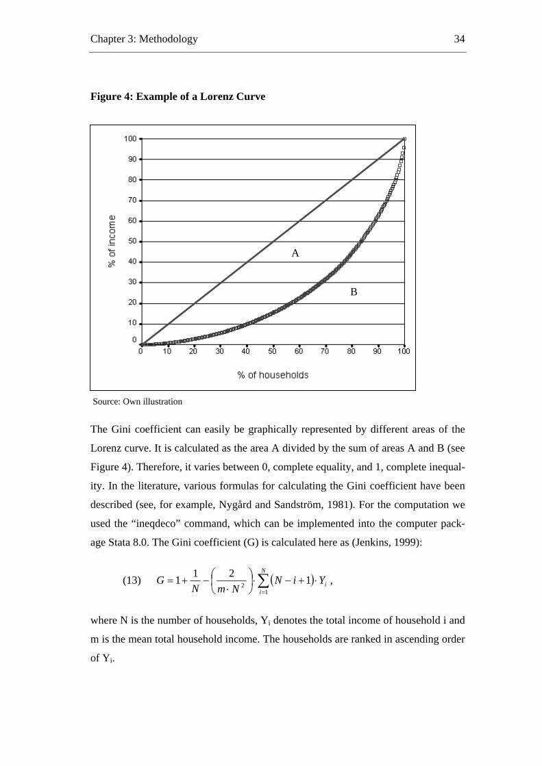
Chapter 3: Methodology
34
Figure 4: Example of a Lorenz Curve
A
B
Source: Own illustration
The Gini coefficient can easily be graphically represented by different areas of the
Lorenz curve. It is calculated as the area A divided by the sum of areas A and B (see
Figure 4). Therefore, it varies between 0, complete equality, and 1, complete inequal-
ity. In the literature, various formulas for calculating the Gini coefficient have been
described (see, for example, Nygård and Sandström, 1981). For the computation we
used the “ineqdeco” command, which can be implemented into the computer pack-
age Stata 8.0. The Gini coefficient (G) is calculated here as (Jenkins, 1999):
(13) ( )∑=
⋅+−⋅⎟⎠⎞
⎜⎝⎛
⋅−+=
N
iiYiN
NmNG
12 1211 ,
where N is the number of households, Yi denotes the total income of household i and
m is the mean total household income. The households are ranked in ascending order
of Yi.
Chapter 3: Methodology
35
3.6 Methodology used in the causal analysis
In the causal analysis, which aims to identify underlying factors influencing
the outcomes, various econometric modelling techniques have been applied depend-
ing on the nature of the dependent variable11. All the results presented are weighed
results by applying the sampling weights presented earlier in this chapter. In contrast
to the coefficient estimates, the standard errors have not been corrected for sampling
effects.
In the descriptive analysis in Chapter 4 and Chapter 5, two observations were
striking outliers. One household has a remarkably high income from self-
employment outside the agricultural sector generating two-thirds of the activity in-
come of all households. Another household gains almost 28% of its total income
from livestock production. As these are highly exceptional cases they have been ex-
cluded from the regression analysis. The number of observations used in the regres-
sion analysis therefore dropped to 291, which is equivalent to a weighed number of
287.
3.6.1 Total household income
To determine the influence of internal and external factors on the total house-
hold income, which is a continuous variable, ordinary least square (OLS) estimation
has been used to estimate the linear model
(14) ( ) µβ += XYln ,
where Y denotes the total household income and x the vector of variables influencing
income. Beta is the vector of coefficients which will be estimated and µ is the unob-
servable random disturbance or error term. Similar models on total household in-
come have been widely used in the literature, for example in Corral and Reardon
11 The programming codes for the various models are available on request from the author
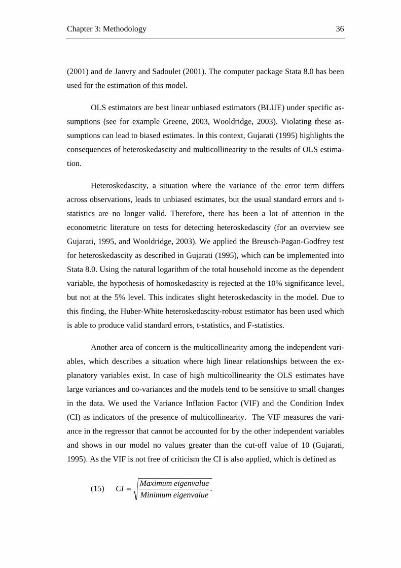
Chapter 3: Methodology
36
(2001) and de Janvry and Sadoulet (2001). The computer package Stata 8.0 has been
used for the estimation of this model.
OLS estimators are best linear unbiased estimators (BLUE) under specific as-
sumptions (see for example Greene, 2003, Wooldridge, 2003). Violating these as-
sumptions can lead to biased estimates. In this context, Gujarati (1995) highlights the
consequences of heteroskedascity and multicollinearity to the results of OLS estima-
tion.
Heteroskedascity, a situation where the variance of the error term differs
across observations, leads to unbiased estimates, but the usual standard errors and t-
statistics are no longer valid. Therefore, there has been a lot of attention in the
econometric literature on tests for detecting heteroskedascity (for an overview see
Gujarati, 1995, and Wooldridge, 2003). We applied the Breusch-Pagan-Godfrey test
for heteroskedascity as described in Gujarati (1995), which can be implemented into
Stata 8.0. Using the natural logarithm of the total household income as the dependent
variable, the hypothesis of homoskedascity is rejected at the 10% significance level,
but not at the 5% level. This indicates slight heteroskedascity in the model. Due to
this finding, the Huber-White heteroskedascity-robust estimator has been used which
is able to produce valid standard errors, t-statistics, and F-statistics.
Another area of concern is the multicollinearity among the independent vari-
ables, which describes a situation where high linear relationships between the ex-
planatory variables exist. In case of high multicollinearity the OLS estimates have
large variances and co-variances and the models tend to be sensitive to small changes
in the data. We used the Variance Inflation Factor (VIF) and the Condition Index
(CI) as indicators of the presence of multicollinearity. The VIF measures the vari-
ance in the regressor that cannot be accounted for by the other independent variables
and shows in our model no values greater than the cut-off value of 10 (Gujarati,
1995). As the VIF is not free of criticism the CI is also applied, which is defined as
(15) .eigenvalueMinimumeigenvalueMaximumCI =
Chapter 3: Methodology
37
In our model the CI is 16, which is well below the cut-off point of 30 suggested by
Belsley et al. (1980).
3.6.2 Participation in income activities
Participation in an income activity is measured by a binary variable which is
zero if the household does not participate in an activity. In this case the income gen-
erated from this activity is a missing value. The binary variable takes on the value
one, if the household generates income from this activity. We are interested in how
the vector of explanatory variables X influences the possibility that the binary de-
pendent variable Y takes on the value 1. The binary response Probit model can be
written as
(16) ( ) ( )XGXYP β== /1 ,
where G(.) is the standard normal density distribution and β the vector of coeffi-
cients, which is estimated by Maximum Likelihood Estimation (MLE). Similar mod-
els on total household income have been widely used in the literature, for example in
Corral and Reardon (2001) and Lanjouw et al. (2001). The computer package Lim-
dep 7.0 has been used for the estimation of this model.
When estimating Probit models it is important to have a sufficient mix of
ones and zeros on your dependent variable. In general, there has to be at least K of
each value, where K is the number of independent variables (Greene, 1998). As this
requirement is not fulfilled for the variable measuring the gender of the head of the
household, it has been dropped from the analysis.
3.6.3 Activity income
In the analysis of activity incomes we distinguish seven different activities:
annual crop production, perennial crop production, livestock production, collection
of forest products, agricultural wage labour, self-employment outside the agricultural
sector, and non-agricultural wage labour.
Chapter 3: Methodology
38
A feature of all these activities is that many households do not participate in
them. The percentage of households participating ranges from 82% in annual crop
production to just 16% in non-agricultural wage labour. Within the random sample of
households, some decide to participate in an activity. If they have chosen to partici-
pate in an activity we can measure the income from it. Since unobserved characteris-
tics of participants, which differentiate them from non-participants, may also have an
influence on the income, estimation of the coefficients may be biased. This bias is
called sample or more precisely self-selection bias (Wooldridge, 2002). The most
common approach used in the literature to account for sample selection is the
Heckman two-step estimator, commonly referred to as the Heckit model. In similar
settings such models have been used, for example in Lanjouw (2001). Sample selec-
tion models are generalisations of Tobit models12. Whereas in Tobit models the se-
lection process is modelled implicitly as being determined by the same variables that
explain income, the Heckman selection model explicitly models the decision to par-
ticipate in an activity and the income generated from this activity in two different
equations (Wooldridge, 2002). Despite this drawback, Tobit models are also used in
the analysis of income activities, as for example in de Janvry and Sadoulet (2001).
Beside the nature of the dependent variables, another distinct feature of activ-
ity choice is its simultaneity. The household does not decide for each activity sepa-
rately whether it should for example, use its resources in this activity. It can choose
to use its assets in different activities at the same time and the choice of an activity is
linked to the other activities and depends on them. To reflect the simultaneity of the
household members’ decision between the different activities, system methods of
estimation like Three-stage least squares (3SLS) estimation, are required. They make
full use of the information contained in the variables of the system because they also
take also into account interactions between them (Greene, 2003).
As the commonly used Heckit model is not able to account for the simultane-
ity of activity choice and in Tobit models the selection process is modelled only im-
plicitly, another approach is followed. Taylor and Yunez-Naude (2000) use a model
12 See next section for a description of Tobit models
Chapter 3: Methodology
39
which considers selectivity as well as simultaneity of activity choice to estimate the
returns of schooling to different activities. Their application involves a simultaneous
equation model in which the dependent variables are censored by unobserved latent
variables. Moreover, they also control for the endogeneity of activity choice. The
econometric approach follows a generalisation by Lee (1978) of an estimation prin-
ciple by Amemiya (1977).
In the first stage a Probit similar to the one described in the previous section
is estimated using the full set of explanatory variables. Based on the Probit estimates,
the activity specific inverse Mills ratios (IMR) are calculated. They are included as
right-hand variables in the corresponding activity income equations and correct for
the endogeneity of activity choice. The system of activity income equations is then
estimated jointly for the full household sample using 3SLS. Hence, we are also able
to exploit the information contained in the cross-equation error terms. Only assets
which are expected to affect the income level of that activity are included as explana-
tory variables in the corresponding income equation. The estimated coefficients are
the absolute effect of one-unit changes in the corresponding explanatory variables on
activity incomes. They are also called selectivity-corrected activity income estimates
(Taylor and Yunez-Naude, 2000). Winters et al. (2002) and Yunez-Naude and Taylor
(2001) used the same approach in similar settings. The computer package Limdep
7.0 has been used for the estimation of this model.
Using the IMR as an instrumental variable to model the endogeneity of the
selection process has been criticised due to problems in identification (see for exam-
ple Deaton, 1997). A high correlation between the explanatory variables used in the
choice and in the income model can lead to collinearity between the IMR and the
other independent variables in the activity income equations. This can make the es-
timation sensitive to small changes in the data (Puhani, 2000). Therefore, we again
used the CI as proposed by Leung and Yu (1996) to detect collinearity. In our model
all the CIs are around 25, which is below the cut-off point of 30 suggested by Belsley
et al. (1980).
Chapter 3: Methodology
40
3.6.4 Income diversity
Both dependent variables measuring income diversity, the share of non-
agricultural income and the Shannon equitability index, are continuous variables but
with a limited range between zero and 100. Moreover, in both cases there is a large
share of observations with zero values meaning that households do not participate in
non-agricultural activities and that they derive their income from one source only,
respectively. Conventional regression methods fail to take into account the qualita-
tive difference between zero and continuous observations. Therefore, we apply Tobit
models which have been originally developed for censored data, but which are also
used for corner solution models (Wooldridge, 2002). The computer package Limdep
7.0 has been used for the estimation of this model.
The Tobit model in case of censoring at zero can be written as
(17) and (18) iii xY µβ +=* ( )*,0max ii YY = .
Yi is the observed censored variable, which is equal to the unobserved latent variable
Yi*, when Yi
* is bigger than zero. In all other cases Yi is equal to zero. The coeffi-
cients are estimated by MLE, where the likelihood consists of the product of expres-
sions for the probability of obtaining each observation. For each observation greater
than zero this expression is just the height of the appropriate density function repre-
senting the probability of getting that particular observation. For observation equal or
smaller than zero it is the probability of getting an observation below or equal zero,
which would be the integral below the limit of the appropriate density function.
The estimated coefficients identify two effects (see Wooldridge, 2002):
1) The effect of an independent variable on the probability of having income for
the non-participating households (the censored observations)
2) The effect of the explanatory variables on the income share for the house-
holds participating
Chapter 3: Methodology
41
These two effects can be distinguished by a decomposition technique proposed by
Mc Donald and Moffit (1980).
Two specification issues are highlighted in the literature (Greene, 2002,
Wooldridge, 2002). Tobit estimates are generally inconsistent if the error terms are
heteroskedastic or distributed non-normal. An informal way to evaluate a Tobit
model is proposed in Wooldridge (2002). He suggests comparing the Probit esti-
mates with the Tobit estimates divided by the disturbance standard deviation σ. The
sign and the magnitudes of the significant explanatory variables should be similar.
This holds true for the Tobit models estimated in this study.
3.7 Summary
This chapter presented the methodology used to answer the research ques-
tions of this study. The sampling frame for the selection of households used the
methods of clustering and stratification. Data was collected through a standardised,
formal questionnaire from 301 randomly selected households in. Due to dispropor-
tional sampling of the households sampling weights are used in the descriptive and
causal analysis. We apply t-test and Analysis of Variance as well as their non-
parametric equivalents, the Mann-Whitney test and the Kruskal-Wallis test, to test
for statistical significant differences among groups in the descriptive analysis. Fur-
thermore, this chapter discussed features and limitations of the econometric models
applied in the causal analysis. The determinants of total household income are esti-
mated using Ordinary Least Squares estimation. Probit models are used to investigate
factors influencing activity choice. In the analysis of activity incomes Lee’s generali-
sation of an estimation principle by Amemiya is applied, which takes into account
simultaneity and endogeneity of activity choice. The chapter ends with a discussion
of Tobit models used in the model on income diversity.
Before going into the causal analysis, the next chapter describes the results of
the descriptive analysis of the incomes and activities engaged by rural households.
Chapter 4
4 Descriptive analysis of income and activities
This chapter presents the results of the descriptive analysis of income and ac-
tivities engaged by rural households. The analysis follows the differentiation of ac-
tivities introduced in the previous chapter according to sectors and functions. More-
over, agricultural self-employment is divided into crop production, livestock produc-
tion and the sale of forest products. This leads to six different income activities dif-
ferentiated throughout this chapter. After illustrating the composition of the total
household income over all households it is shown how this mixture changes accord-
ing to different socio-economic groups. The different activities are then explored in
detail with special emphasis on regional differences. After evaluating income shares
and the degree of income specialisation, the final section looks at the distribution of
income.
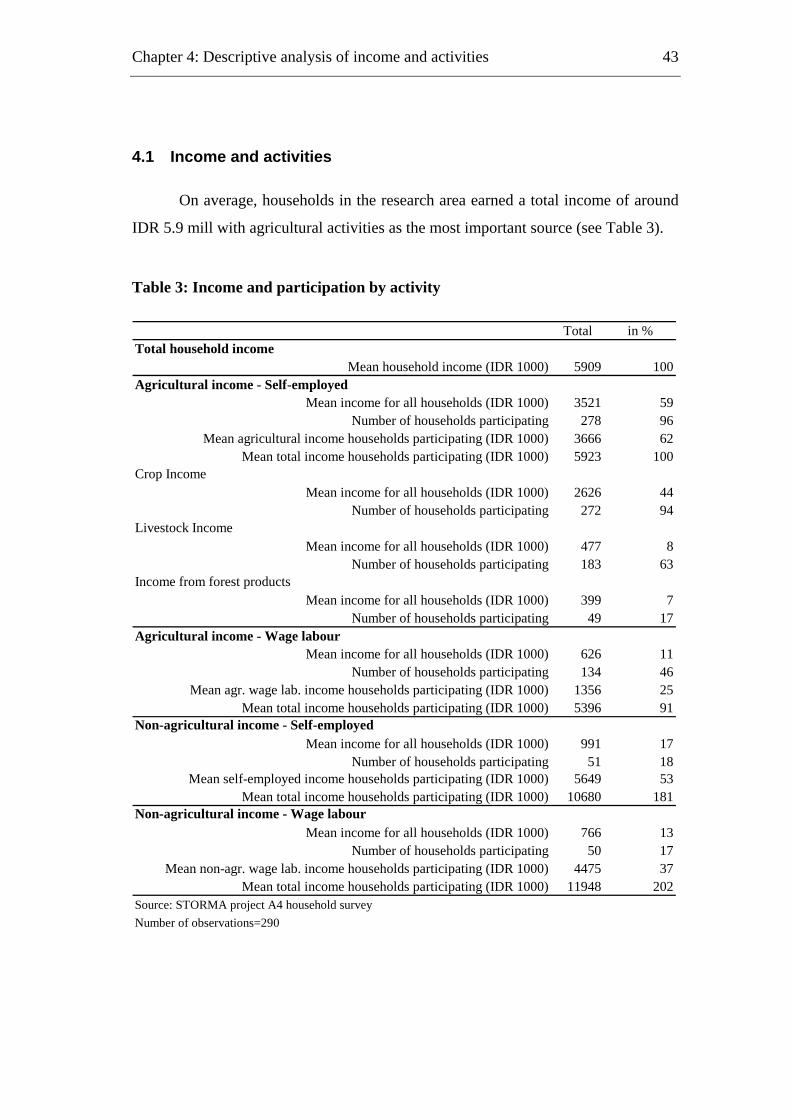
Chapter 4: Descriptive analysis of income and activities
43
4.1 Income and activities
On average, households in the research area earned a total income of around
IDR 5.9 mill with agricultural activities as the most important source (see Table 3).
Table 3: Income and participation by activity
Total in %Total household income
Mean household income (IDR 1000) 5909 100Agricultural income - Self-employed
Mean income for all households (IDR 1000) 3521 59Number of households participating 278 96
Mean agricultural income households participating (IDR 1000) 3666 62Mean total income households participating (IDR 1000) 5923 100
Crop IncomeMean income for all households (IDR 1000) 2626 44
Number of households participating 272 94Livestock Income
Mean income for all households (IDR 1000) 477 8Number of households participating 183 63
Income from forest productsMean income for all households (IDR 1000) 399 7
Number of households participating 49 17Agricultural income - Wage labour
Mean income for all households (IDR 1000) 626 11Number of households participating 134 46
Mean agr. wage lab. income households participating (IDR 1000) 1356 25Mean total income households participating (IDR 1000) 5396 91
Non-agricultural income - Self-employedMean income for all households (IDR 1000) 991 17
Number of households participating 51 18Mean self-employed income households participating (IDR 1000) 5649 53
Mean total income households participating (IDR 1000) 10680 181Non-agricultural income - Wage labour
Mean income for all households (IDR 1000) 766 13Number of households participating 50 17
Mean non-agr. wage lab. income households participating (IDR 1000) 4475 37Mean total income households participating (IDR 1000) 11948 202
Source: STORMA project A4 household surveyNumber of observations=290

Chapter 4: Descriptive analysis of income and activities
44
Agricultural self-employment and wage labour activities together contribute
to 70% of total household income, with the remaining 30% coming from non-
agricultural activities. This confirms findings of a literature review by Reardon et al.
(1998) reporting that about 35% of rural incomes in Indonesia stem from non-
agricultural activities. However, a study from the sub district of Lampung, Indonesia,
reported a non-agricultural income share of only 20% (Jatileksono, 1994), indicating
large differences between regions. The most important activity is crop production,
which accounts for about 44% of the total income. This is followed by income from
enterprises and rents (17%) and non-agricultural wage labour (13%). However, par-
ticipation of the households in the latter activities is much lower. Of the 290 house-
holds, only 51, which is equivalent to 18%, reported income from non-agricultural
self-employment. In the case of wage labour activities outside agriculture, just 50
households earned income from this activity. In contrast, 94% take part in cropping
activities. But income from non-agricultural activities is a much more important in-
come source for participating households. The 51 households with income from non-
agricultural self-employment gained on average IDR 5.6 mill from this activity,
which is equivalent to 53% of their total household income of IDR 10.7 mill. More-
over, their total household income is 81% higher than the average income of IDR 5.9
mill. The same applies for non-agricultural wage labour income: participating house-
holds generate 37% of their total income from this activity and their total household
income is 102% higher than that of the average household.
Non-agricultural income accounts for almost one-third of the total household
income over all groups, but how does this change if we look at different wealth
groups? Applying the poverty index introduced in Chapter 3, Table 4 shows incomes
and activities differentiated by poverty terciles: poorest (poverty group 1), poor
(poverty group 3), and less-poor households (poverty group 3).
Statistically significant differences between socio-economic groups exist in
the total household income as well as in all the activity incomes except in the income
from agricultural wage labour. The average income of poverty group 3 is more than
three times higher than the average income of poverty group 1. The differences are

Chapter 4: Descriptive analysis of income and activities
45
even more striking in the case of incomes from non-agricultural activities. Less-poor
households generate on average 23 times more income from non-agricultural self-
employment and 6 times more from non-agricultural wage labour than the poorest
households.
Moreover, the number of households participating is also statistically differ-
ent between socio-economic groups for all activities except agricultural self-
employment. Participation in agricultural wage labour activities is comparatively low
for households that are better off, whereas it is the other way round for non-
agricultural activities. In non-agricultural self-employment 26% and in non-
agricultural wage employment 25% of the less-poor households participate. In con-
trast, only 7% of the poorest households are engaged in non-agricultural self-
employment and only 10% participate in non-agricultural wage labour activities.
Table 4: Income and participation by activity and poverty group
Poverty GroupTotal in % Total in % Total in %
Total household incomeMean total household income (IDR 1000) 3619 100 3807 100 11134 100
N 102 100 102 100 86 100Agricultural income - Self-employed
Mean income (IDR 1000) 2643 73 2044 54 6320 57Number of households participating 98 96 98 96 82 95
Crop incomeMean income (IDR 1000) 1668 46 1636 43 4940 44
Number of households participating 93 92 97 95 82 95Livestock income
Mean income (IDR 1000) 213 6 109 3 1228 11Number of households participating 74 73 53 52 56 65
Income from forest productsMean income (IDR 1000) 755 21 260 7 140 1
Number of households participating 31 30 15 14 4 4Agricultural income - Wage labour
Mean income (IDR 1000) 631 17 714 19 516 5Number of households participating 48 47 59 58 27 31
Non-agricultural income - Self-employedMean income (IDR 1000) 116 3 393 10 2744 25
Number of households participating 7 7 22 21 22 26Non-agricultural income - Wage labour
Mean income (IDR 1000) 223 6 653 17 1547 14Number of households participating 10 10 18 18 21 25
Source: STORMA project A4 household surveyNumber of observations=290
31 2
Chapter 4: Descriptive analysis of income and activities
46
These differences are also reflected in the percentage shares in total income
by activity13. Own account agricultural activities are the most important income
source for all socio-economic groups, but for the poorest households it contributes
almost three-quarters to their total household income. For the other groups it ac-
counts for only 54% and 57%, respectively. The same also applies for agricultural
wage labour income. It is most important for the poorest households and less impor-
tant for the poor and less-poor households. For income derived from outside the agri-
cultural sector it is the other way round. It is particularly important for households
that are better off. They generate 25% of their total household income from self-
employment outside agriculture, whereas it accounts for only 3% of the income of
the poorest households. In the case of non-agricultural wage labour income the pic-
ture is not as clear, as it plays an important role especially for poverty group two.
This can be explained by the different types of non-agricultural wage labour activi-
ties which are a mix of unskilled jobs like working in construction, and skilled jobs
like teachers.
An important activity for the poorest households is the selling of forest prod-
ucts and fishing: 32% of them participate in these activities generating 21% of their
total household income. For the poor households it accounts for only 7% and for the
non-poor this income source is no longer relevant.
4.2 Agricultural self-employed income
Agricultural self-employed income consists of all own-account activities
within the agricultural sector, which is income from crops, livestock, and fishing and
forest products.
13 These shares are calculated as the mean activity income over all households divided by the mean of
total household income over all households. Therefore it is not possible to apply statistical tests on
differences between socio-economic groups.
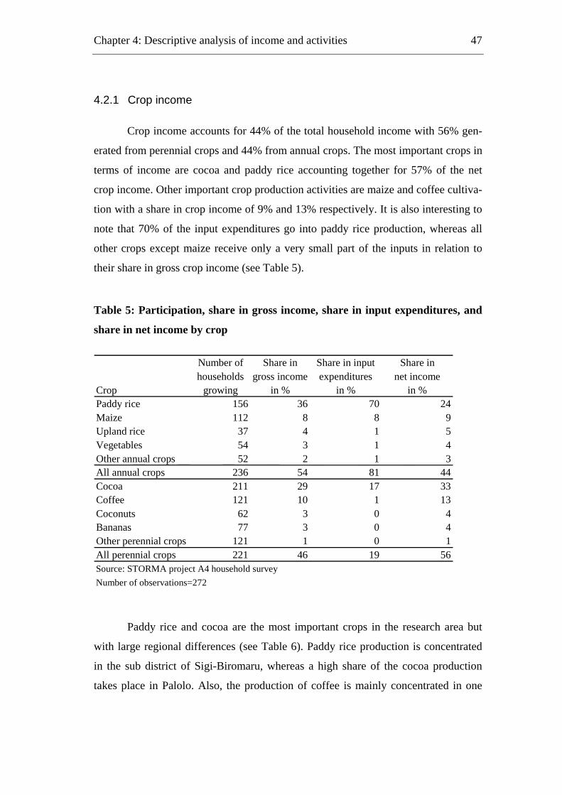
Chapter 4: Descriptive analysis of income and activities
47
4.2.1 Crop income
Crop income accounts for 44% of the total household income with 56% gen-
erated from perennial crops and 44% from annual crops. The most important crops in
terms of income are cocoa and paddy rice accounting together for 57% of the net
crop income. Other important crop production activities are maize and coffee cultiva-
tion with a share in crop income of 9% and 13% respectively. It is also interesting to
note that 70% of the input expenditures go into paddy rice production, whereas all
other crops except maize receive only a very small part of the inputs in relation to
their share in gross crop income (see Table 5).
Table 5: Participation, share in gross income, share in input expenditures, and
share in net income by crop
Number of Share in Share in input Share in households gross income expenditures net income
Crop growing in % in % in % Paddy rice 156 36 70 24 Maize 112 8 8 9 Upland rice 37 4 1 5 Vegetables 54 3 1 4 Other annual crops 52 2 1 3 All annual crops 236 54 81 44 Cocoa 211 29 17 33 Coffee 121 10 1 13 Coconuts 62 3 0 4 Bananas 77 3 0 4 Other perennial crops 121 1 0 1 All perennial crops 221 46 19 56 Source: STORMA project A4 household survey Number of observations=272
Paddy rice and cocoa are the most important crops in the research area but
with large regional differences (see Table 6). Paddy rice production is concentrated
in the sub district of Sigi-Biromaru, whereas a high share of the cocoa production
takes place in Palolo. Also, the production of coffee is mainly concentrated in one
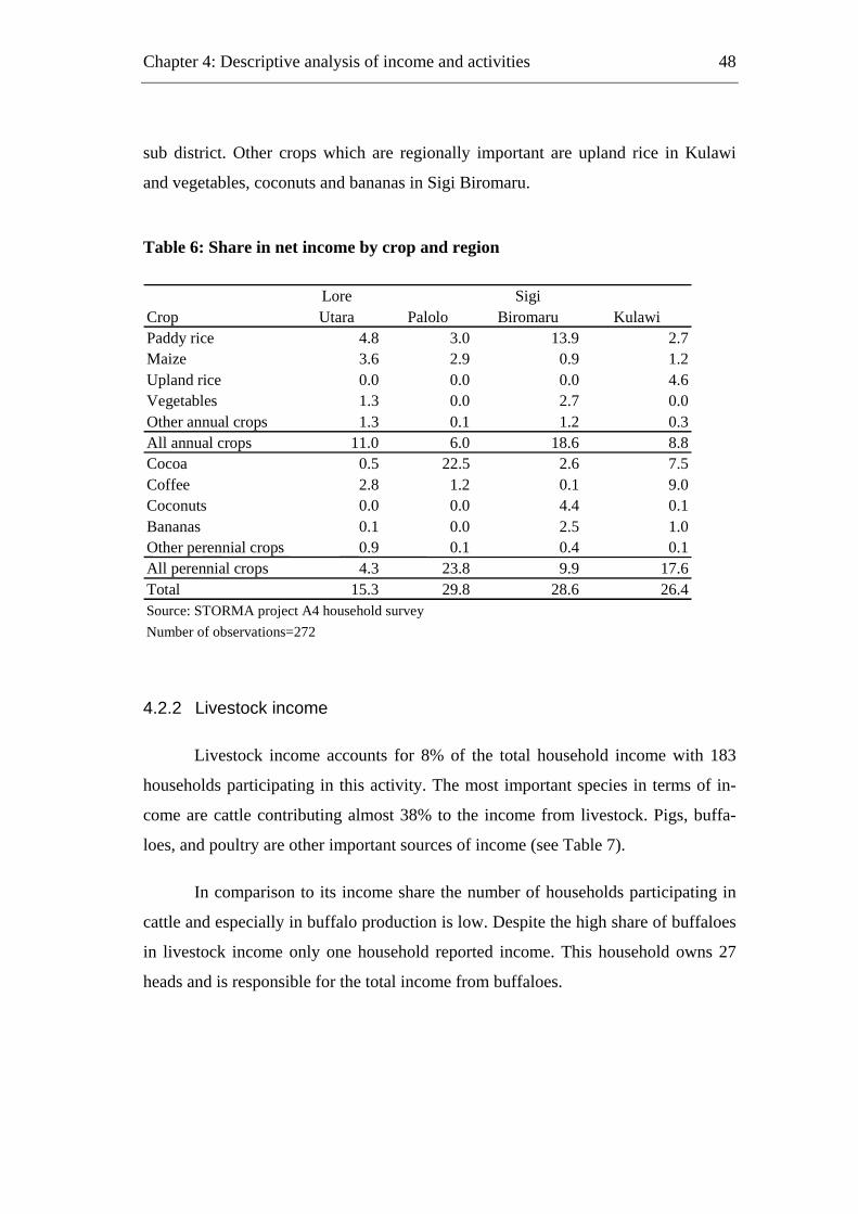
Chapter 4: Descriptive analysis of income and activities
48
sub district. Other crops which are regionally important are upland rice in Kulawi
and vegetables, coconuts and bananas in Sigi Biromaru.
Table 6: Share in net income by crop and region
Lore SigiCrop Utara Palolo Biromaru Kulawi Paddy rice 4.8 3.0 13.9 2.7 Maize 3.6 2.9 0.9 1.2 Upland rice 0.0 0.0 0.0 4.6 Vegetables 1.3 0.0 2.7 0.0 Other annual crops 1.3 0.1 1.2 0.3 All annual crops 11.0 6.0 18.6 8.8 Cocoa 0.5 22.5 2.6 7.5 Coffee 2.8 1.2 0.1 9.0 Coconuts 0.0 0.0 4.4 0.1 Bananas 0.1 0.0 2.5 1.0 Other perennial crops 0.9 0.1 0.4 0.1 All perennial crops 4.3 23.8 9.9 17.6 Total 15.3 29.8 28.6 26.4 Source: STORMA project A4 household survey Number of observations=272
4.2.2 Livestock income
Livestock income accounts for 8% of the total household income with 183
households participating in this activity. The most important species in terms of in-
come are cattle contributing almost 38% to the income from livestock. Pigs, buffa-
loes, and poultry are other important sources of income (see Table 7).
In comparison to its income share the number of households participating in
cattle and especially in buffalo production is low. Despite the high share of buffaloes
in livestock income only one household reported income. This household owns 27
heads and is responsible for the total income from buffaloes.
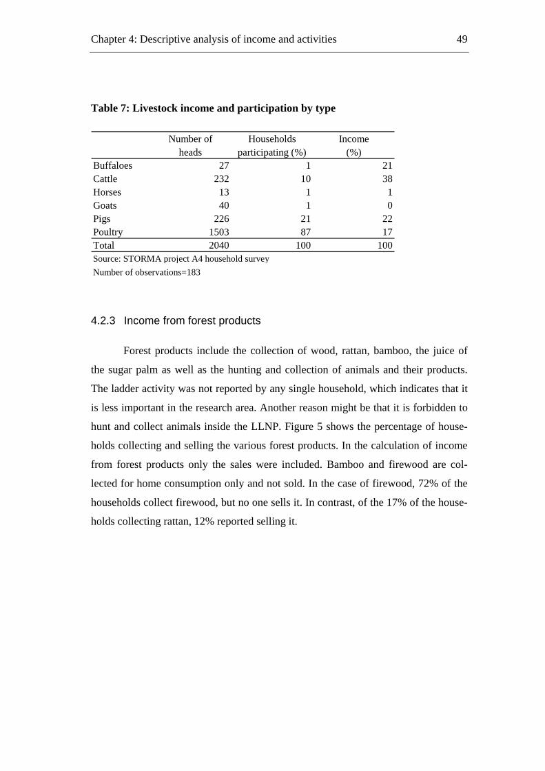
Chapter 4: Descriptive analysis of income and activities
49
Table 7: Livestock income and participation by type
Number of Households Incomeheads participating (%) (%)
Buffaloes 27 1 21 Cattle 232 10 38 Horses 13 1 1 Goats 40 1 0 Pigs 226 21 22 Poultry 1503 87 17 Total 2040 100 100 Source: STORMA project A4 household surveyNumber of observations=183
4.2.3 Income from forest products
Forest products include the collection of wood, rattan, bamboo, the juice of
the sugar palm as well as the hunting and collection of animals and their products.
The ladder activity was not reported by any single household, which indicates that it
is less important in the research area. Another reason might be that it is forbidden to
hunt and collect animals inside the LLNP. Figure 5 shows the percentage of house-
holds collecting and selling the various forest products. In the calculation of income
from forest products only the sales were included. Bamboo and firewood are col-
lected for home consumption only and not sold. In the case of firewood, 72% of the
households collect firewood, but no one sells it. In contrast, of the 17% of the house-
holds collecting rattan, 12% reported selling it.

Chapter 4: Descriptive analysis of income and activities
50
Figure 5: Collection and sale of forest products
72
1217 15 15
0 0
12
04
0
10
20
30
40
50
60
70
80
Firewood Wood forconstruction
Rattan Bamboo Juice ofsugar palm
% o
f hou
seho
lds
collectionsale
Source: STORMA project A4 household survey. Number of observations = 290
The sale of forest products accounts for 7% of the total household income
with almost three-quarters originating from the sale of rattan. Around 20% of the
income originates from selling the juice of the sugar palm and the remainder from
selling wood for construction (see Figure 6).
Figure 6: Income from the sale of forest products by product
6.1
73.5
20.4
Wood for construction
Rattan
Juice of sugar palm
Source: STORMA project A4 household survey. Number of observations = 49
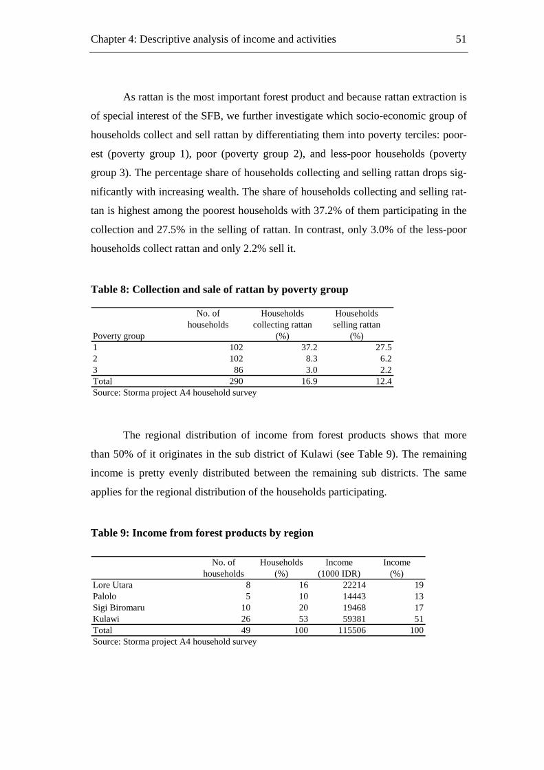
Chapter 4: Descriptive analysis of income and activities
51
As rattan is the most important forest product and because rattan extraction is
of special interest of the SFB, we further investigate which socio-economic group of
households collect and sell rattan by differentiating them into poverty terciles: poor-
est (poverty group 1), poor (poverty group 2), and less-poor households (poverty
group 3). The percentage share of households collecting and selling rattan drops sig-
nificantly with increasing wealth. The share of households collecting and selling rat-
tan is highest among the poorest households with 37.2% of them participating in the
collection and 27.5% in the selling of rattan. In contrast, only 3.0% of the less-poor
households collect rattan and only 2.2% sell it.
Table 8: Collection and sale of rattan by poverty group
No. of Households Householdshouseholds collecting rattan selling rattan
Poverty group (%) (%)1 102 37.2 27.52 102 8.3 6.23 86 3.0Total 290 16.9 12.4Source: Storma project A4 household survey
2.2
The regional distribution of income from forest products shows that more
than 50% of it originates in the sub district of Kulawi (see Table 9). The remaining
income is pretty evenly distributed between the remaining sub districts. The same
applies for the regional distribution of the households participating.
Table 9: Income from forest products by region
No. of Households Income Incomehouseholds (%) (1000 IDR) (%)
Lore Utara 8 16 22214 19Palolo 5 10 14443 13Sigi Biromaru 10 20 19468 17Kulawi 26 53 59381 51Total 49 100 115506 100Source: Storma project A4 household survey

Chapter 4: Descriptive analysis of income and activities
52
4.3 Self-employed income outside agriculture
Income from self-employment outside the agricultural sector accounts for
17% of the total household income with 18% of the households participating. The
most important source is trade, accounting for 57% of the income from self-
employment, but with only six households participating (see Table 10). One wood
trader alone generates more than two-thirds of the total self-employed income out-
side agriculture. Other important activities are shops/food stalls and small-scale in-
dustries which generate 23% and 12% of the income from this activity.
Table 10: Self-employed income outside agriculture by activity
Number of Households Income Income Mean incomehouseholds (%) (IDR 1000) (%) (IDR 1000)
Shop/warung 23 37 65873 23 2904Craft 8 13 8323 3 1249Trader 6 10 164744 57 36543Small Scale Industry 11 17 33667 12 2961Other 2 3 5292 2 4381Renting 13 21 9344 3 778Total 63 100 287243 100 4559Source: STORMA project A4 household surveyNumber of observations=51
The regional distribution shows that participation is highest in the sub district
of Sigi Biromaru with 32 households engaged (see Table 11). This sub district has
the highest population density and the best infrastructure, for example the most dense
road network. The regional distribution in terms of income is highly biased by the
above-mentioned trader, so that 61% of the income from self-employment is gener-
ated in the sub district of Palolo alone.
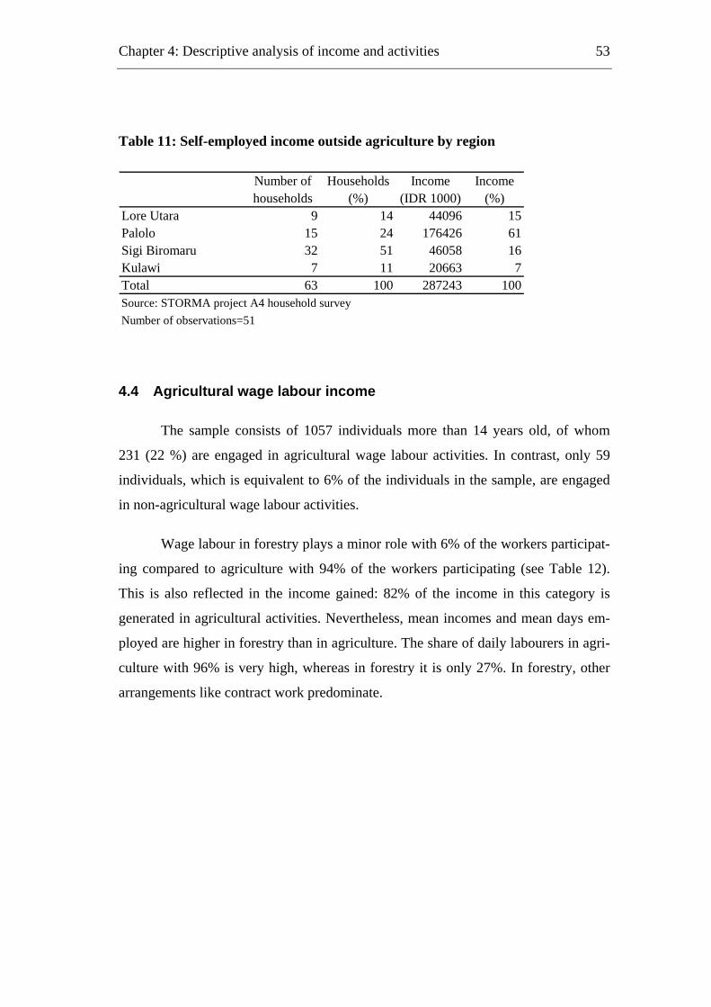
Chapter 4: Descriptive analysis of income and activities
53
Table 11: Self-employed income outside agriculture by region
Number of Households Income Incomehouseholds (%) (IDR 1000) (%)
Lore Utara 9 14 44096 15Palolo 15 24 176426 61Sigi Biromaru 32 51 46058 16Kulawi 7 11 20663 7Total 63 100 287243 100Source: STORMA project A4 household surveyNumber of observations=51
4.4 Agricultural wage labour income
The sample consists of 1057 individuals more than 14 years old, of whom
231 (22 %) are engaged in agricultural wage labour activities. In contrast, only 59
individuals, which is equivalent to 6% of the individuals in the sample, are engaged
in non-agricultural wage labour activities.
Wage labour in forestry plays a minor role with 6% of the workers participat-
ing compared to agriculture with 94% of the workers participating (see Table 12).
This is also reflected in the income gained: 82% of the income in this category is
generated in agricultural activities. Nevertheless, mean incomes and mean days em-
ployed are higher in forestry than in agriculture. The share of daily labourers in agri-
culture with 96% is very high, whereas in forestry it is only 27%. In forestry, other
arrangements like contract work predominate.
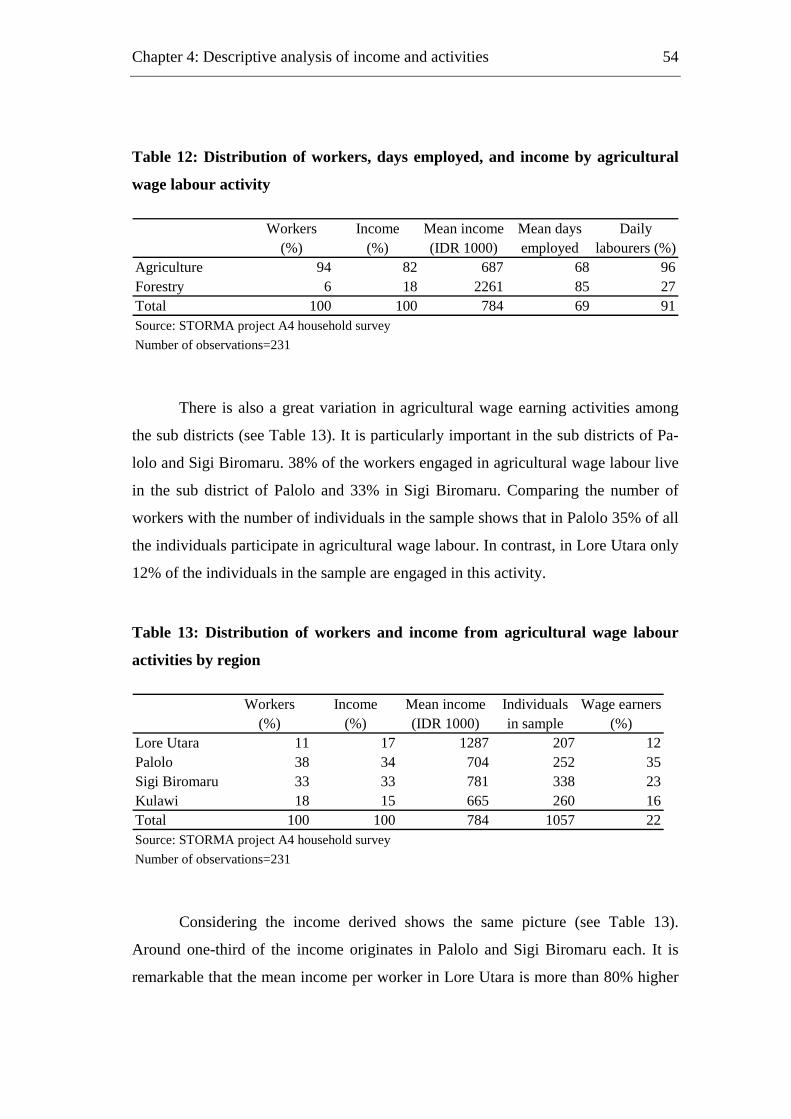
Chapter 4: Descriptive analysis of income and activities
54
Table 12: Distribution of workers, days employed, and income by agricultural
wage labour activity
Workers Income Mean income Mean days Daily(%) (%) (IDR 1000) employed labourers (%)
Agriculture 94 82 687 68 96Forestry 6 18 2261 85 27Total 100 100 784 69 91Source: STORMA project A4 household surveyNumber of observations=231
There is also a great variation in agricultural wage earning activities among
the sub districts (see Table 13). It is particularly important in the sub districts of Pa-
lolo and Sigi Biromaru. 38% of the workers engaged in agricultural wage labour live
in the sub district of Palolo and 33% in Sigi Biromaru. Comparing the number of
workers with the number of individuals in the sample shows that in Palolo 35% of all
the individuals participate in agricultural wage labour. In contrast, in Lore Utara only
12% of the individuals in the sample are engaged in this activity.
Table 13: Distribution of workers and income from agricultural wage labour
activities by region
Workers Income Mean income Individuals Wage earners(%) (%) (IDR 1000) in sample (%)
Lore Utara 11 17 1287 207 12Palolo 38 34 704 252 35Sigi Biromaru 33 33 781 338 23Kulawi 18 15 665 260 16Total 100 100 784 1057 22Source: STORMA project A4 household surveyNumber of observations=231
Considering the income derived shows the same picture (see Table 13).
Around one-third of the income originates in Palolo and Sigi Biromaru each. It is
remarkable that the mean income per worker in Lore Utara is more than 80% higher
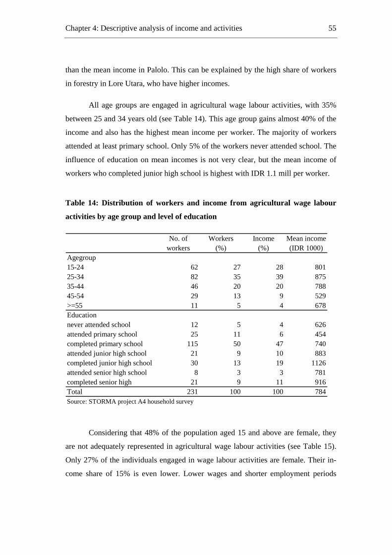
Chapter 4: Descriptive analysis of income and activities
55
than the mean income in Palolo. This can be explained by the high share of workers
in forestry in Lore Utara, who have higher incomes.
All age groups are engaged in agricultural wage labour activities, with 35%
between 25 and 34 years old (see Table 14). This age group gains almost 40% of the
income and also has the highest mean income per worker. The majority of workers
attended at least primary school. Only 5% of the workers never attended school. The
influence of education on mean incomes is not very clear, but the mean income of
workers who completed junior high school is highest with IDR 1.1 mill per worker.
Table 14: Distribution of workers and income from agricultural wage labour
activities by age group and level of education
No. of Workers Income Mean incomeworkers (%) (%) (IDR 1000)
Agegroup15-24 62 27 28 80125-34 82 35 39 87535-44 46 20 20 78845-54 29 13 9 529>=55 11 5 4 678Educationnever attended school 12 5 4 626attended primary school 25 11 6 454completed primary school 115 50 47 740attended junior high school 21 9 10 883completed junior high school 30 13 19 1126attended senior high school 8 3 3 781completed senior high 21 9 11 916Total 231 100 100 784Source: STORMA project A4 household survey
Considering that 48% of the population aged 15 and above are female, they
are not adequately represented in agricultural wage labour activities (see Table 15).
Only 27% of the individuals engaged in wage labour activities are female. Their in-
come share of 15% is even lower. Lower wages and shorter employment periods
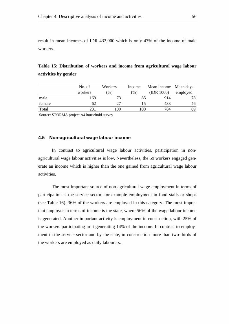
Chapter 4: Descriptive analysis of income and activities
56
result in mean incomes of IDR 433,000 which is only 47% of the income of male
workers.
Table 15: Distribution of workers and income from agricultural wage labour
activities by gender
No. of Workers Income Mean income Mean daysworkers (%) (%) (IDR 1000) employed
male 169 73 85 914 78female 62 27 15 433 46Total 231 100 100 784 69Source: STORMA project A4 household survey
4.5 Non-agricultural wage labour income
In contrast to agricultural wage labour activities, participation in non-
agricultural wage labour activities is low. Nevertheless, the 59 workers engaged gen-
erate an income which is higher than the one gained from agricultural wage labour
activities.
The most important source of non-agricultural wage employment in terms of
participation is the service sector, for example employment in food stalls or shops
(see Table 16). 36% of the workers are employed in this category. The most impor-
tant employer in terms of income is the state, where 56% of the wage labour income
is generated. Another important activity is employment in construction, with 25% of
the workers participating in it generating 14% of the income. In contrast to employ-
ment in the service sector and by the state, in construction more than two-thirds of
the workers are employed as daily labourers.
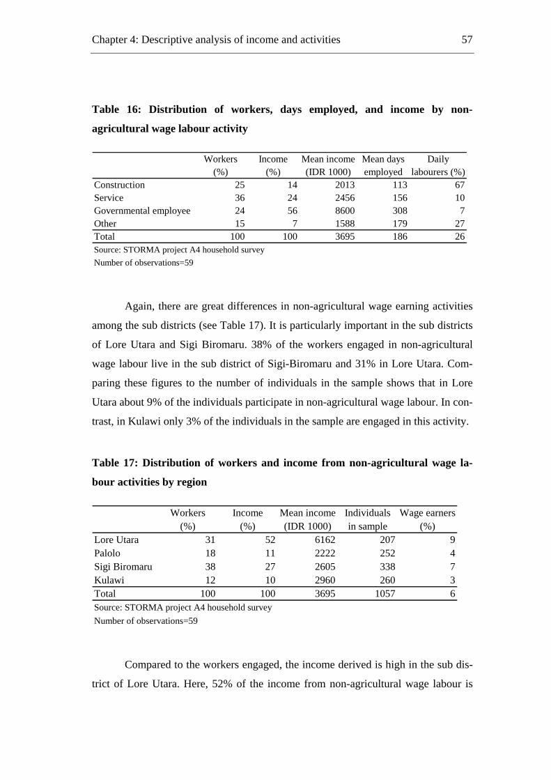
Chapter 4: Descriptive analysis of income and activities
57
Table 16: Distribution of workers, days employed, and income by non-
agricultural wage labour activity
Workers Income Mean income Mean days Daily(%) (%) (IDR 1000) employed labourers (%)
Construction 25 14 2013 113 67Service 36 24 2456 156 10Governmental employee 24 56 8600 308 7Other 15 7 1588 179 27Total 100 100 3695 186 26Source: STORMA project A4 household surveyNumber of observations=59
Again, there are great differences in non-agricultural wage earning activities
among the sub districts (see Table 17). It is particularly important in the sub districts
of Lore Utara and Sigi Biromaru. 38% of the workers engaged in non-agricultural
wage labour live in the sub district of Sigi-Biromaru and 31% in Lore Utara. Com-
paring these figures to the number of individuals in the sample shows that in Lore
Utara about 9% of the individuals participate in non-agricultural wage labour. In con-
trast, in Kulawi only 3% of the individuals in the sample are engaged in this activity.
Table 17: Distribution of workers and income from non-agricultural wage la-
bour activities by region
Workers Income Mean income Individuals Wage earners(%) (%) (IDR 1000) in sample (%)
Lore Utara 31 52 6162 207 9Palolo 18 11 2222 252 4Sigi Biromaru 38 27 2605 338 7Kulawi 12 10 2960 260 3Total 100 100 3695 1057 6Source: STORMA project A4 household surveyNumber of observations=59
Compared to the workers engaged, the income derived is high in the sub dis-
trict of Lore Utara. Here, 52% of the income from non-agricultural wage labour is
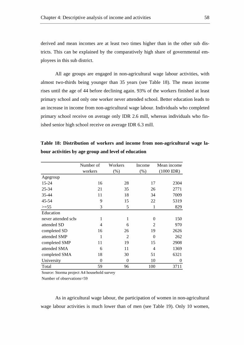
Chapter 4: Descriptive analysis of income and activities
58
derived and mean incomes are at least two times higher than in the other sub dis-
tricts. This can be explained by the comparatively high share of governmental em-
ployees in this sub district.
All age groups are engaged in non-agricultural wage labour activities, with
almost two-thirds being younger than 35 years (see Table 18). The mean income
rises until the age of 44 before declining again. 93% of the workers finished at least
primary school and only one worker never attended school. Better education leads to
an increase in income from non-agricultural wage labour. Individuals who completed
primary school receive on average only IDR 2.6 mill, whereas individuals who fin-
ished senior high school receive on average IDR 6.3 mill.
Table 18: Distribution of workers and income from non-agricultural wage la-
bour activities by age group and level of education
Number of Workers Income Mean incomeworkers (%) (%) (1000 IDR)
Agegroup15-24 16 28 17 230425-34 21 35 26 277135-44 11 18 34 700945-54 9 15 22 5319>=55 3 5 1 829Educationnever attended scho 1 1 0attended SD 4 6 2 970completed SD 16 26 19 2626attended SMP 1 2 0 262completed SMP 11 19 15 2908attended SMA 6 11 4 1369completed SMA 18 30 51 6321University 0 0 10 0Total 59 96 100 3711Source: Storma project A4 household surveyNumber of observations=59
150
As in agricultural wage labour, the participation of women in non-agricultural
wage labour activities is much lower than of men (see Table 19). Only 10 women,
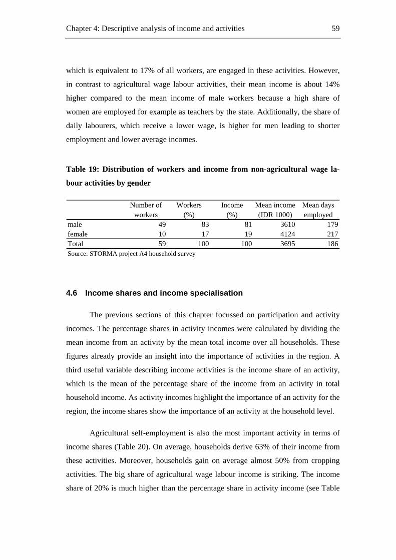
Chapter 4: Descriptive analysis of income and activities
59
which is equivalent to 17% of all workers, are engaged in these activities. However,
in contrast to agricultural wage labour activities, their mean income is about 14%
higher compared to the mean income of male workers because a high share of
women are employed for example as teachers by the state. Additionally, the share of
daily labourers, which receive a lower wage, is higher for men leading to shorter
employment and lower average incomes.
Table 19: Distribution of workers and income from non-agricultural wage la-
bour activities by gender
Number of Workers Income Mean income Mean daysworkers (%) (%) (IDR 1000) employed
male 49 83 81 3610 179female 10 17 19 4124 217Total 59 100 100 3695 186Source: STORMA project A4 household survey
4.6 Income shares and income specialisation
The previous sections of this chapter focussed on participation and activity
incomes. The percentage shares in activity incomes were calculated by dividing the
mean income from an activity by the mean total income over all households. These
figures already provide an insight into the importance of activities in the region. A
third useful variable describing income activities is the income share of an activity,
which is the mean of the percentage share of the income from an activity in total
household income. As activity incomes highlight the importance of an activity for the
region, the income shares show the importance of an activity at the household level.
Agricultural self-employment is also the most important activity in terms of
income shares (Table 20). On average, households derive 63% of their income from
these activities. Moreover, households gain on average almost 50% from cropping
activities. The big share of agricultural wage labour income is striking. The income
share of 20% is much higher than the percentage share in activity income (see Table
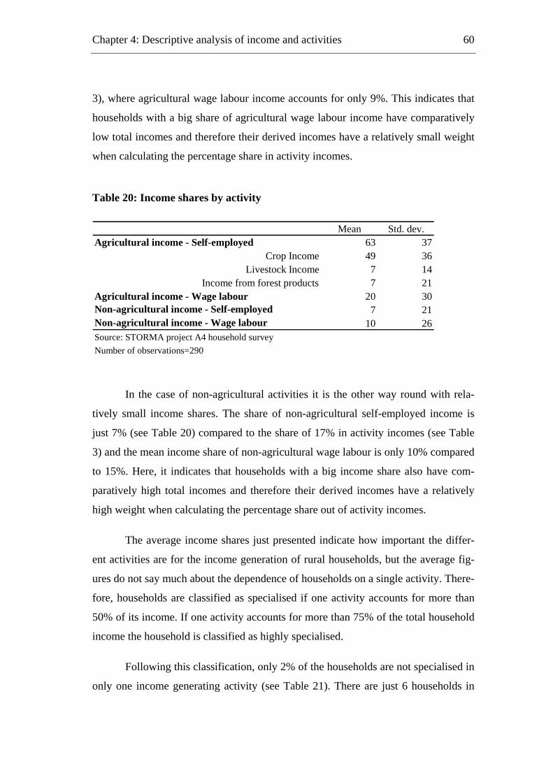
Chapter 4: Descriptive analysis of income and activities
60
3), where agricultural wage labour income accounts for only 9%. This indicates that
households with a big share of agricultural wage labour income have comparatively
low total incomes and therefore their derived incomes have a relatively small weight
when calculating the percentage share in activity incomes.
Table 20: Income shares by activity
Mean Std. dev. Agricultural income - Self-employed 63 37
Crop Income 49 36 Livestock Income 7 14
Income from forest products 7 21 Agricultural income - Wage labour 20 30 Non-agricultural income - Self-employed 7 21 Non-agricultural income - Wage labour 10 26 Source: STORMA project A4 household survey Number of observations=290
In the case of non-agricultural activities it is the other way round with rela-
tively small income shares. The share of non-agricultural self-employed income is
just 7% (see Table 20) compared to the share of 17% in activity incomes (see Table
3) and the mean income share of non-agricultural wage labour is only 10% compared
to 15%. Here, it indicates that households with a big income share also have com-
paratively high total incomes and therefore their derived incomes have a relatively
high weight when calculating the percentage share out of activity incomes.
The average income shares just presented indicate how important the differ-
ent activities are for the income generation of rural households, but the average fig-
ures do not say much about the dependence of households on a single activity. There-
fore, households are classified as specialised if one activity accounts for more than
50% of its income. If one activity accounts for more than 75% of the total household
income the household is classified as highly specialised.
Following this classification, only 2% of the households are not specialised in
only one income generating activity (see Table 21). There are just 6 households in
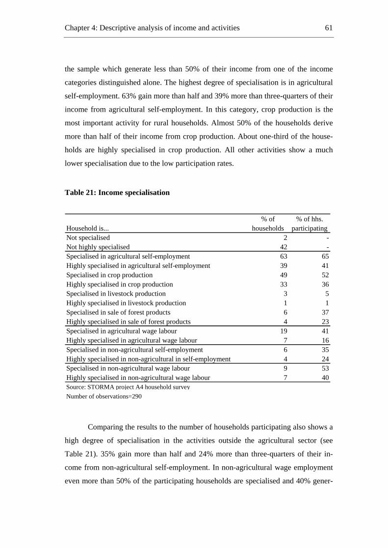
Chapter 4: Descriptive analysis of income and activities
61
the sample which generate less than 50% of their income from one of the income
categories distinguished alone. The highest degree of specialisation is in agricultural
self-employment. 63% gain more than half and 39% more than three-quarters of their
income from agricultural self-employment. In this category, crop production is the
most important activity for rural households. Almost 50% of the households derive
more than half of their income from crop production. About one-third of the house-
holds are highly specialised in crop production. All other activities show a much
lower specialisation due to the low participation rates.
Table 21: Income specialisation
% of % of hhs.Household is... households participatingNot specialised 2 -Not highly specialised 42 -Specialised in agricultural self-employment 63 65Highly specialised in agricultural self-employment 39 41Specialised in crop production 49 52Highly specialised in crop production 33 36Specialised in livestock production 3 5Highly specialised in livestock production 1 1Specialised in sale of forest products 6 37Highly specialised in sale of forest products 4 23Specialised in agricultural wage labour 19 41Highly specialised in agricultural wage labour 7 16Specialised in non-agricultural self-employment 6 35Highly specialised in non-agricultural in self-employment 4 24Specialised in non-agricultural wage labour 9 53Highly specialised in non-agricultural wage labour 7 40Source: STORMA project A4 household surveyNumber of observations=290
Comparing the results to the number of households participating also shows a
high degree of specialisation in the activities outside the agricultural sector (see
Table 21). 35% gain more than half and 24% more than three-quarters of their in-
come from non-agricultural self-employment. In non-agricultural wage employment
even more than 50% of the participating households are specialised and 40% gener-
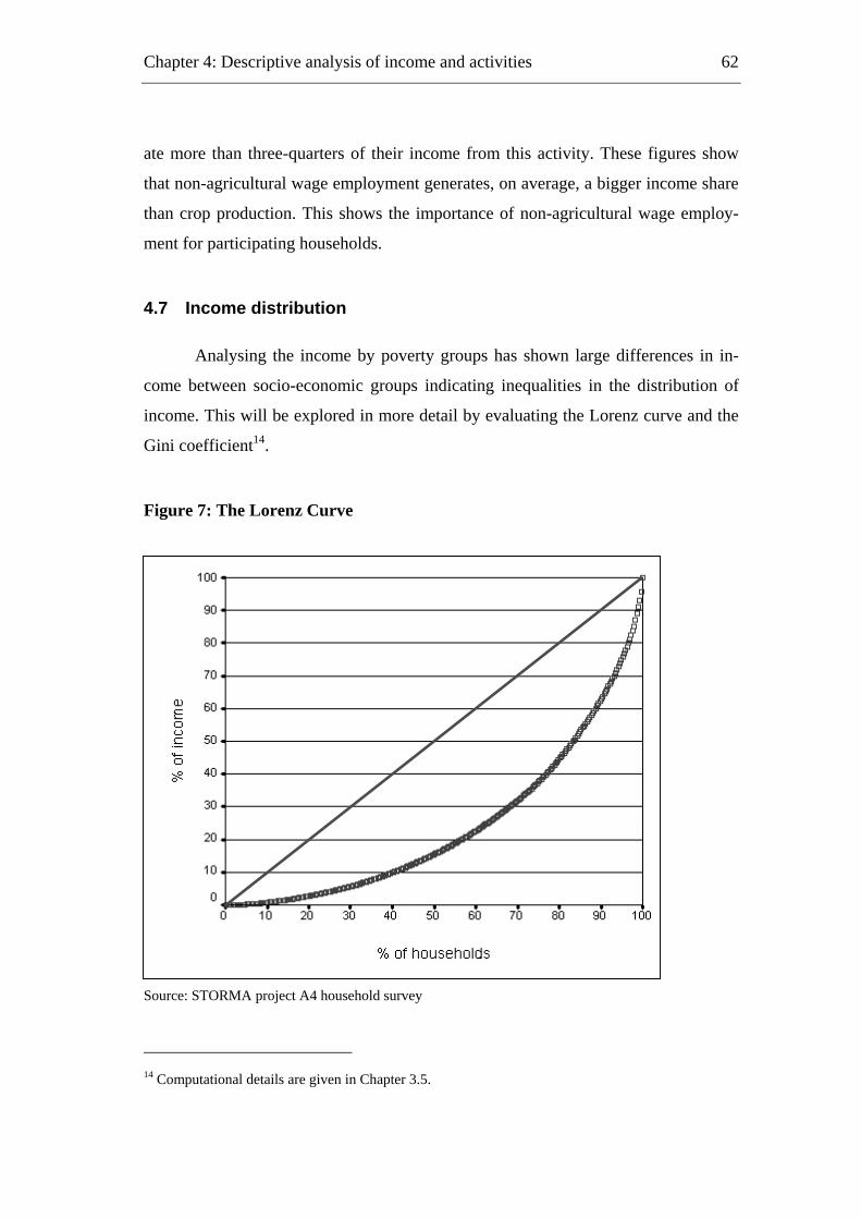
Chapter 4: Descriptive analysis of income and activities
62
ate more than three-quarters of their income from this activity. These figures show
that non-agricultural wage employment generates, on average, a bigger income share
than crop production. This shows the importance of non-agricultural wage employ-
ment for participating households.
4.7 Income distribution
Analysing the income by poverty groups has shown large differences in in-
come between socio-economic groups indicating inequalities in the distribution of
income. This will be explored in more detail by evaluating the Lorenz curve and the
Gini coefficient14.
Figure 7: The Lorenz Curve
Source: STORMA project A4 household survey
14 Computational details are given in Chapter 3.5.
Chapter 4: Descriptive analysis of income and activities
63
The Lorenz curve (see Figure 7) as well as the Gini coefficient, which is 0.52,
show a rather unequal distribution of income among the households. Comparing the
Gini coefficient measured with other sources is rather difficult because most of them
used data on consumption expenditures per capita. An exception is Asra (2000), who
calculated Gini coefficients based on household income. For the whole of Indonesia
as well as rural areas only, the Gini coefficient dropped from 0.51 in 1977 to 0.43 in
1982 (Asra, 2000). Figures for the period after 1982 have not been found.
4.8 Summary
This chapter presented the results of the descriptive analysis of income and
activities. Agricultural activities are the most important source of income for rural
households in the region contributing to 70% of total household income. The remain-
ing 30% originates from non-agricultural activities indicating its importance. How-
ever, participation in the latter activities is much lower with just around 18% com-
pared to 96% in agricultural activities. Differentiation between different wealth
groups shows that activities outside the agricultural sector are particularly important
for the less-poor households. Within agricultural activities the most important source
of income is crop production with the most important crops being irrigated rice and
cocoa. Nevertheless, large regional differences exist. After the analysis of activity
participation and incomes we focus on income shares describing the importance of
activities at the household level. The share of non-agricultural income of 7% is much
lower than its share in activity income. This indicates that households with a high
share of non-agricultural income also have a comparatively high total income. Based
on the income shares we evaluated the dependence of households on a single activ-
ity. Only 2% of the households generate less than 50% of their income from one
source. In contrast, 39% of the households generate more than three-quarters of their
income from a single activity indicating a specialisation of households. Applying a
Lorenz curve in the last section of this chapter shows a rather uneven distribution of
income among the households.
Chapter 4: Descriptive analysis of income and activities
64
Before analysing the factors influencing the described variables by economet-
ric modelling they need to be further evaluated. The next chapter presents the de-
scriptive analysis of the influencing factors introduced in Chapter 2.
Chapter 5
5 Descriptive analysis of factors influencing income and activity choice
Before analysing the influencing factors on participation and incomes by
econometric modelling it is necessary to further evaluate these factors. This chapter
describes the socio-economic factors influencing activity choice and incomes intro-
duced in the conceptual framework. Emphasis is placed on the variables, which are
included in the econometric models in the next chapter. After analysing the posses-
sion of land and its differences between regions, other assets owned by rural house-
holds are described in the first section of this chapter. The demographic structure of
rural households and the educational background of its members are then described.
The third section describes the access to social capital, the pattern of migration and
the ethnic composition. After evaluating the participation in credit markets the last
section in this chapter briefly describes the access to road infrastructure.

Chapter 5: Descriptive analysis of factors influencing income and activity choice
66
5.1 Physical capital
Physical capital consists of land, livestock, and other assets. As the posses-
sion of livestock has been already described in the previous chapter the analysis here
is limited to the other two categories of physical capital.
5.1.1 Possession of land
Households in the research area own on average 1.8 ha of land, but with sta-
tistically significant differences among the sub districts (see Table 22). Households
in the sub district of Lore Utara own on average 2.7 ha, whereas households in Sigi
Biromaru possess just above one hectare. As we will see later, these variations can be
explained by the qualitative differences of the land.
Table 22: Share of land owned by sub district
Lore SigiUtara Palolo Biromaru Kulawi Total
zero ha 0.0 9.5 5.7 1.0 4.50 - 1 ha 20.3 23.8 48.6 23.4 32.01 - 2 ha 27.0 37.2 32.0 30.2 31.92 - 3 ha 20.9 10.5 6.3 21.4 13.43 - 4 ha 10.9 10.5 4.9 3.5 6.94 - 5ha 4.8 1.9 0.0 12.7 4.3>= 5 ha 16.1 6.7 2.4 7.7 7.0
Mean land owned in ha 2.7 1.8 1.1 2.3 1.8Source: STORMA project A4 household surveyNumber of observations=290
The share of households owing no land at all is 4.5% ranging from zero per-
cent in the sub district of Lore Utara to almost 10% in Palolo (see Table 22). These
households rent or borrow their homestead and all the land they cultivate. Almost
one-third of the households own less than one hectare in the region and around two-
thirds own less than two hectares. The high share of households owning more than
five hectares in Lore Utara is remarkable.
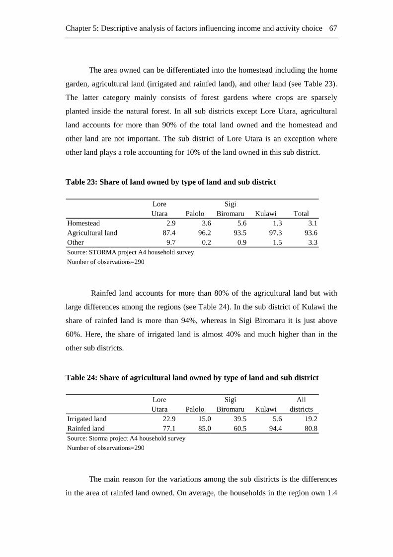
Chapter 5: Descriptive analysis of factors influencing income and activity choice
67
The area owned can be differentiated into the homestead including the home
garden, agricultural land (irrigated and rainfed land), and other land (see Table 23).
The latter category mainly consists of forest gardens where crops are sparsely
planted inside the natural forest. In all sub districts except Lore Utara, agricultural
land accounts for more than 90% of the total land owned and the homestead and
other land are not important. The sub district of Lore Utara is an exception where
other land plays a role accounting for 10% of the land owned in this sub district.
Table 23: Share of land owned by type of land and sub district
Lore SigiUtara Palolo Biromaru Kulawi Total
Homestead 2.9 3.6 5.6 1.3 3.1Agricultural land 87.4 96.2 93.5 97.3 93.6Other 9.7 0.2 0.9 1.5 3.3Source: STORMA project A4 household surveyNumber of observations=290
Rainfed land accounts for more than 80% of the agricultural land but with
large differences among the regions (see Table 24). In the sub district of Kulawi the
share of rainfed land is more than 94%, whereas in Sigi Biromaru it is just above
60%. Here, the share of irrigated land is almost 40% and much higher than in the
other sub districts.
Table 24: Share of agricultural land owned by type of land and sub district
Lore Sigi AllUtara Palolo Biromaru Kulawi districts
Irrigated land 22.9 15.0 39.5 5.6 19.2Rainfed land 77.1 85.0 60.5 94.4 80.8Source: Storma project A4 household surveyNumber of observations=290
The main reason for the variations among the sub districts is the differences
in the area of rainfed land owned. On average, the households in the region own 1.4
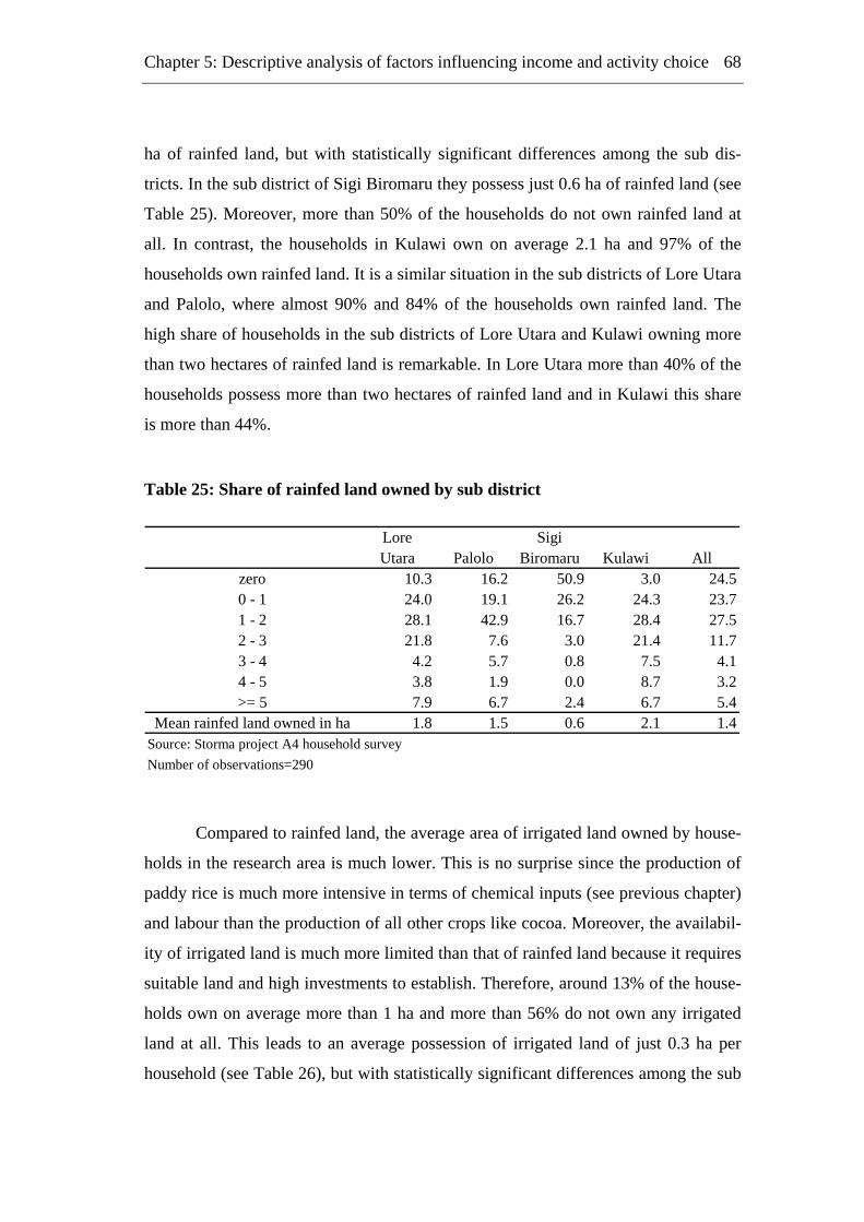
Chapter 5: Descriptive analysis of factors influencing income and activity choice
68
ha of rainfed land, but with statistically significant differences among the sub dis-
tricts. In the sub district of Sigi Biromaru they possess just 0.6 ha of rainfed land (see
Table 25). Moreover, more than 50% of the households do not own rainfed land at
all. In contrast, the households in Kulawi own on average 2.1 ha and 97% of the
households own rainfed land. It is a similar situation in the sub districts of Lore Utara
and Palolo, where almost 90% and 84% of the households own rainfed land. The
high share of households in the sub districts of Lore Utara and Kulawi owning more
than two hectares of rainfed land is remarkable. In Lore Utara more than 40% of the
households possess more than two hectares of rainfed land and in Kulawi this share
is more than 44%.
Table 25: Share of rainfed land owned by sub district
Lore SigiUtara Palolo Biromaru Kulawi All
zero 10.3 16.2 50.9 3.0 24.50 - 1 24.0 19.1 26.2 24.3 23.71 - 2 28.1 42.9 16.7 28.4 27.52 - 3 21.8 7.6 3.0 21.4 11.73 - 4 4.2 5.7 0.8 7.5 4.14 - 5 3.8 1.9 0.0 8.7 3.2>= 5 7.9 6.7 2.4 6.7 5.4
Mean rainfed land owned in ha 1.8 1.5 0.6 2.1 1.4Source: Storma project A4 household surveyNumber of observations=290
Compared to rainfed land, the average area of irrigated land owned by house-
holds in the research area is much lower. This is no surprise since the production of
paddy rice is much more intensive in terms of chemical inputs (see previous chapter)
and labour than the production of all other crops like cocoa. Moreover, the availabil-
ity of irrigated land is much more limited than that of rainfed land because it requires
suitable land and high investments to establish. Therefore, around 13% of the house-
holds own on average more than 1 ha and more than 56% do not own any irrigated
land at all. This leads to an average possession of irrigated land of just 0.3 ha per
household (see Table 26), but with statistically significant differences among the sub
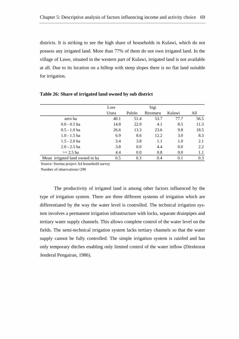
Chapter 5: Descriptive analysis of factors influencing income and activity choice
69
districts. It is striking to see the high share of households in Kulawi, which do not
possess any irrigated land. More than 77% of them do not own irrigated land. In the
village of Lawe, situated in the western part of Kulawi, irrigated land is not available
at all. Due to its location on a hilltop with steep slopes there is no flat land suitable
for irrigation.
Table 26: Share of irrigated land owned by sub district
Lore SigiUtara Palolo Biromaru Kulawi All
zero ha 40.1 51.4 53.7 77.7 56.50.0 - 0.5 ha 14.8 22.9 4.1 8.5 11.30.5 - 1.0 ha 26.6 13.3 23.6 9.8 18.51.0 - 1.5 ha 6.9 8.6 12.2 3.0 8.31.5 - 2.0 ha 3.4 3.8 1.1 1.0 2.12.0 - 2.5 ha 3.8 0.0 4.4 0.0 2.2>= 2.5 ha 4.4 0.0 0.8 0.0 1.1
Mean irrigated land owned in ha 0.5 0.3 0.4 0.1 0.3Source: Storma project A4 household surveyNumber of observations=290
The productivity of irrigated land is among other factors influenced by the
type of irrigation system. There are three different systems of irrigation which are
differentiated by the way the water level is controlled. The technical irrigation sys-
tem involves a permanent irrigation infrastructure with locks, separate drainpipes and
tertiary water supply channels. This allows complete control of the water level on the
fields. The semi-technical irrigation system lacks tertiary channels so that the water
supply cannot be fully controlled. The simple irrigation system is rainfed and has
only temporary ditches enabling only limited control of the water inflow (Direktorat
Jenderal Pengairan, 1986).
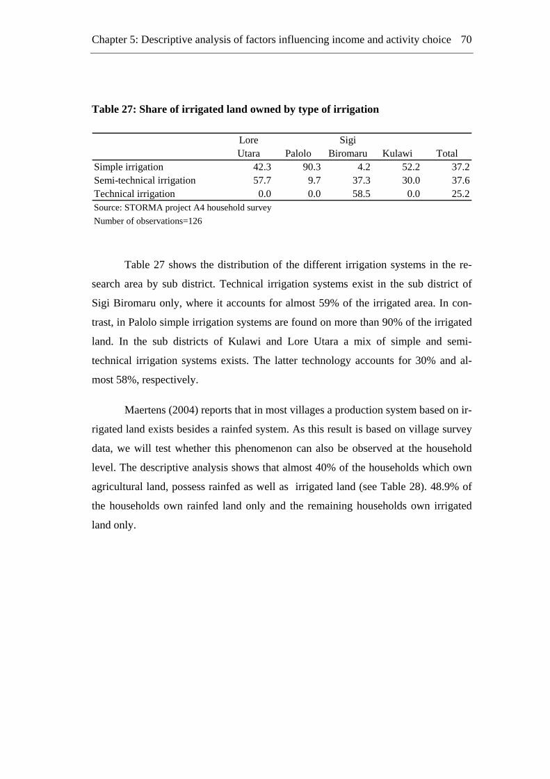
Chapter 5: Descriptive analysis of factors influencing income and activity choice
70
Table 27: Share of irrigated land owned by type of irrigation
Lore SigiUtara Palolo Biromaru Kulawi Total
Simple irrigation 42.3 90.3 4.2 52.2 37.2Semi-technical irrigation 57.7 9.7 37.3 30.0 37.6Technical irrigation 0.0 0.0 58.5 0.0 25.2Source: STORMA project A4 household surveyNumber of observations=126
Table 27 shows the distribution of the different irrigation systems in the re-
search area by sub district. Technical irrigation systems exist in the sub district of
Sigi Biromaru only, where it accounts for almost 59% of the irrigated area. In con-
trast, in Palolo simple irrigation systems are found on more than 90% of the irrigated
land. In the sub districts of Kulawi and Lore Utara a mix of simple and semi-
technical irrigation systems exists. The latter technology accounts for 30% and al-
most 58%, respectively.
Maertens (2004) reports that in most villages a production system based on ir-
rigated land exists besides a rainfed system. As this result is based on village survey
data, we will test whether this phenomenon can also be observed at the household
level. The descriptive analysis shows that almost 40% of the households which own
agricultural land, possess rainfed as well as irrigated land (see Table 28). 48.9% of
the households own rainfed land only and the remaining households own irrigated
land only.
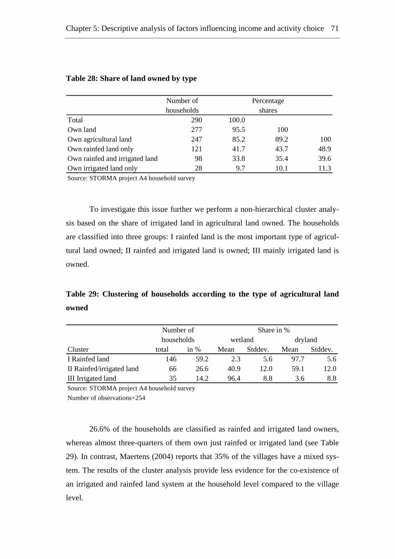
Chapter 5: Descriptive analysis of factors influencing income and activity choice
71
Table 28: Share of land owned by type
Number ofhouseholds
Total 290 100.0Own land 277 95.5 100 Own agricultural land 247 85.2 89.2 100Own rainfed land only 121 41.7 43.7 48.9Own rainfed and irrigated land 98 33.8 35.4 39.6Own irrigated land only 28 9.7 10.1 11.3Source: STORMA project A4 household survey
Percentage shares
To investigate this issue further we perform a non-hierarchical cluster analy-
sis based on the share of irrigated land in agricultural land owned. The households
are classified into three groups: I rainfed land is the most important type of agricul-
tural land owned; II rainfed and irrigated land is owned; III mainly irrigated land is
owned.
Table 29: Clustering of households according to the type of agricultural land
owned
Cluster total in % Mean Stddev. Mean Stddev.I Rainfed land 146 59.2 2.3 5.6 97.7 5.6II Rainfed/irrigated land 66 26.6 40.9 12.0 59.1 12.0III Irrigated land 35 14.2 96.4 8.8 3.6 8.8Source: STORMA project A4 household survey Number of observations=254
Number ofhouseholds
Share in % wetland dryland
26.6% of the households are classified as rainfed and irrigated land owners,
whereas almost three-quarters of them own just rainfed or irrigated land (see Table
29). In contrast, Maertens (2004) reports that 35% of the villages have a mixed sys-
tem. The results of the cluster analysis provide less evidence for the co-existence of
an irrigated and rainfed land system at the household level compared to the village
level.
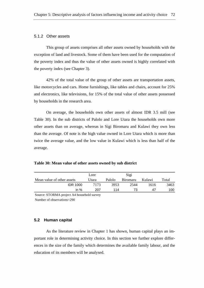
Chapter 5: Descriptive analysis of factors influencing income and activity choice
72
5.1.2 Other assets
This group of assets comprises all other assets owned by households with the
exception of land and livestock. Some of them have been used for the computation of
the poverty index and thus the value of other assets owned is highly correlated with
the poverty index (see Chapter 3).
42% of the total value of the group of other assets are transportation assets,
like motorcycles and cars. Home furnishings, like tables and chairs, account for 25%
and electronics, like televisions, for 15% of the total value of other assets possessed
by households in the research area.
On average, the households own other assets of almost IDR 3.5 mill (see
Table 30). In the sub districts of Palolo and Lore Utara the households own more
other assets than on average, whereas in Sigi Biromaru and Kulawi they own less
than the average. Of note is the high value owned in Lore Utara which is more than
twice the average value, and the low value in Kulawi which is less than half of the
average.
Table 30: Mean value of other assets owned by sub district
Lore SigiMean value of other assets Utara Palolo Biromaru Kulawi Total
IDR 1000 7173 3953 2544 1616 3463in % 207 114 73 47 100
Source: STORMA project A4 household surveyNumber of observations=290
5.2 Human capital
As the literature review in Chapter 1 has shown, human capital plays an im-
portant role in determining activity choice. In this section we further explore differ-
ences in the size of the family which determines the available family labour, and the
education of its members will be analysed.
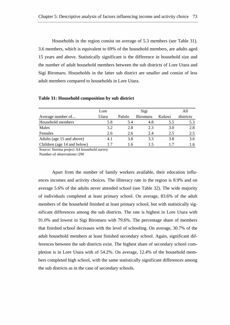
Chapter 5: Descriptive analysis of factors influencing income and activity choice
73
Households in the region consist on average of 5.3 members (see Table 31).
3.6 members, which is equivalent to 69% of the household members, are adults aged
15 years and above. Statistically significant is the difference in household size and
the number of adult household members between the sub districts of Lore Utara and
Sigi Biromaru. Households in the latter sub district are smaller and consist of less
adult members compared to households in Lore Utara.
Table 31: Household composition by sub district
Lore Sigi AllAverage number of... Utara Palolo Biromaru Kulawi districtsHousehold members 5.8 5.4 4.8 5.5 5.3Males 3.2 2.8 2.3 3.0 2.8Females 2.6 2.6 2.4 2.5 2.5Adults (age 15 and above) 4.1 3.8 3.3 3.8 3.6Children (age 14 and below) 1.7 1.6 1.5 1.7 1.6Source: Storma project A4 household surveyNumber of observations=290
Apart from the number of family workers available, their education influ-
ences incomes and activity choices. The illiteracy rate in the region is 8.9% and on
average 5.6% of the adults never attended school (see Table 32). The wide majority
of individuals completed at least primary school. On average, 83.6% of the adult
members of the household finished at least primary school, but with statistically sig-
nificant differences among the sub districts. The rate is highest in Lore Utara with
91.0% and lowest in Sigi Biromaru with 79.6%. The percentage share of members
that finished school decreases with the level of schooling. On average, 30.7% of the
adult household members at least finished secondary school. Again, significant dif-
ferences between the sub districts exist. The highest share of secondary school com-
pletion is in Lore Utara with of 54.2%. On average, 12.4% of the household mem-
bers completed high school, with the same statistically significant differences among
the sub districts as in the case of secondary schools.
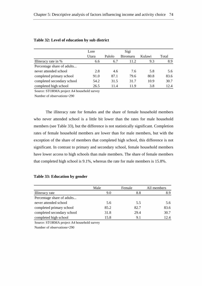
Chapter 5: Descriptive analysis of factors influencing income and activity choice
74
Table 32: Level of education by sub district
Lore SigiUtara Palolo Biromaru Kulawi Total
Illiteracy rate in % 6.6 6.7 11.2 9.3 8.9Percentage share of adults...never attended school 2.8 4.6 7.6 5.8 5.6completed primary school 91.0 87.1 79.6 80.8 83.6completed secondary school 54.2 31.5 31.7 10.9 30.7completed high school 26.5 11.4 11.9 3.8 12.4Source: STORMA project A4 household surveyNumber of observations=290
The illiteracy rate for females and the share of female household members
who never attended school is a little bit lower than the rates for male household
members (see Table 33), but the difference is not statistically significant. Completion
rates of female household members are lower than for male members, but with the
exception of the share of members that completed high school, this difference is not
significant. In contrast to primary and secondary school, female household members
have lower access to high schools than male members. The share of female members
that completed high school is 9.1%, whereas the rate for male members is 15.8%.
Table 33: Education by gender
Male Female All members Illiteracy rate 9.0 8.8 8.9Percentage share of adults... never attended school 5.6 5.5 5.6completed primary school 85.2 82.7 83.6completed secondary school 31.8 29.4 30.7completed high school 15.8 9.1 12.4Source: STORMA project A4 household survey Number of observations=290

Chapter 5: Descriptive analysis of factors influencing income and activity choice
75
5.3 Social capital
Social capital measures the access to social networks and institutions. These
include all kinds of formal institutions, like farmers associations, sport groups, and
religious groups. Moreover, we also asked the members to self-evaluate how active
they were in decision-making processes of these organisations. Besides membership
of formal organisations, the ethnic affiliation and the time the household has lived in
the village are also evaluated since they can influence access to informal networks.
Groups and organisations considered here are, for example, religious groups,
farmer organisations, and neighbourhood groups. On average, households are mem-
bers of 2.8 different organisations (see Table 34). The number of memberships per
adult household member is 0.8. 23% of the households are not members of any or-
ganisation. The number of memberships is statistically significantly higher in Lore
Utara compared to all other sub districts. Moreover, in Lore Utara the number of
memberships is significantly higher than in Kulawi and Palolo and the share of
households without any membership is significantly lower than in Sigi Biromaru.
Table 34: Membership in organisations by sub district
Lore SigiUtara Palolo Biromaru Kulawi Total
Number of memberships 4.4 2.0 2.8 2.3 2.8Number of membershipsper capita 1.1 0.5 0.9 0.6 0.8% of households withoutany membership 9 24 29 22 2Source: STORMA project A4 household surveyNumber of observations=290
3
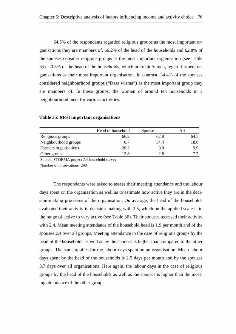
Chapter 5: Descriptive analysis of factors influencing income and activity choice
76
64.5% of the respondents regarded religious groups as the most important or-
ganisations they are members of. 66.2% of the head of the households and 62.8% of
the spouses consider religious groups as the most important organisation (see Table
35). 20.3% of the head of the households, which are mainly men, regard farmers or-
ganisations as their most important organisation. In contrast, 34.4% of the spouses
considered neighbourhood groups (“Dasa wisma”) as the most important group they
are members of. In these groups, the women of around ten households in a
neighbourhood meet for various activities.
Table 35: Most important organisations
Head of household Spouse All Religious groups 66.2 62.8 64.5Neighbourhood groups 0.7 34.4 18.0Farmers organisations 20.3 0.0 9.9Other groups 12.8 2.8 7.7Source: STORMA project A4 household survey Number of observations=290
The respondents were asked to assess their meeting attendance and the labour
days spent on the organisation as well as to estimate how active they are in the deci-
sion-making processes of the organisation. On average, the head of the households
evaluated their activity in decision-making with 2.5, which on the applied scale is in
the range of active to very active (see Table 36). Their spouses assessed their activity
with 2.4. Mean meeting attendance of the household head is 1.9 per month and of the
spouses 2.4 over all groups. Meeting attendance in the case of religious groups by the
head of the households as well as by the spouses is higher than compared to the other
groups. The same applies for the labour days spent on an organisation. Mean labour
days spent by the head of the households is 2.9 days per month and by the spouses
3.7 days over all organisations. Here again, the labour days in the case of religious
groups by the head of the households as well as the spouses is higher than the meet-
ing attendance of the other groups.

Chapter 5: Descriptive analysis of factors influencing income and activity choice
77
Table 36: Meeting attendance, activity in decision-making, and labour days
spent in the most important organisation
Meeting attendance Decision making Labour days spentper month index* per month
Head of household Religious groups 2.5 2.5 3.9
Neighbourhood groups 0.3 3.0 0.5Farmers organisations 0.8 2.4 1.0
Other groups 0.6 2.6 0.9All groups 1.9 2.5 2.9
Spouse Religious groups 3.1 2.5 4.8
Neighbourhood groups 1.3 2.3 2.0Farmers organisations - - -
Other groups 0.8 2.0 1.1All groups 2.4 2.4 3.7
Source: STORMA project A4 household survey Number of observations=290 * 1: less active; 2: active; 3: very active
Besides membership of formal organisations and groups, the ethnic affiliation
can also be seen as social capital. Nevertheless, the influence of ethnicity is much
wider than providing additional access to networks. Traditions are influenced by the
ethnic group the household belongs to, e.g., land use.
80.2% of the households are categorised as indigenous households, with Kaili
and Kulawi being the biggest group (see Table 37). Both account for more than 68%
of the households in the research area. 19.8% of the households are classified as non-
indigenous, with the Bugis as the biggest ethnic group accounting for 8.3% of the
households.
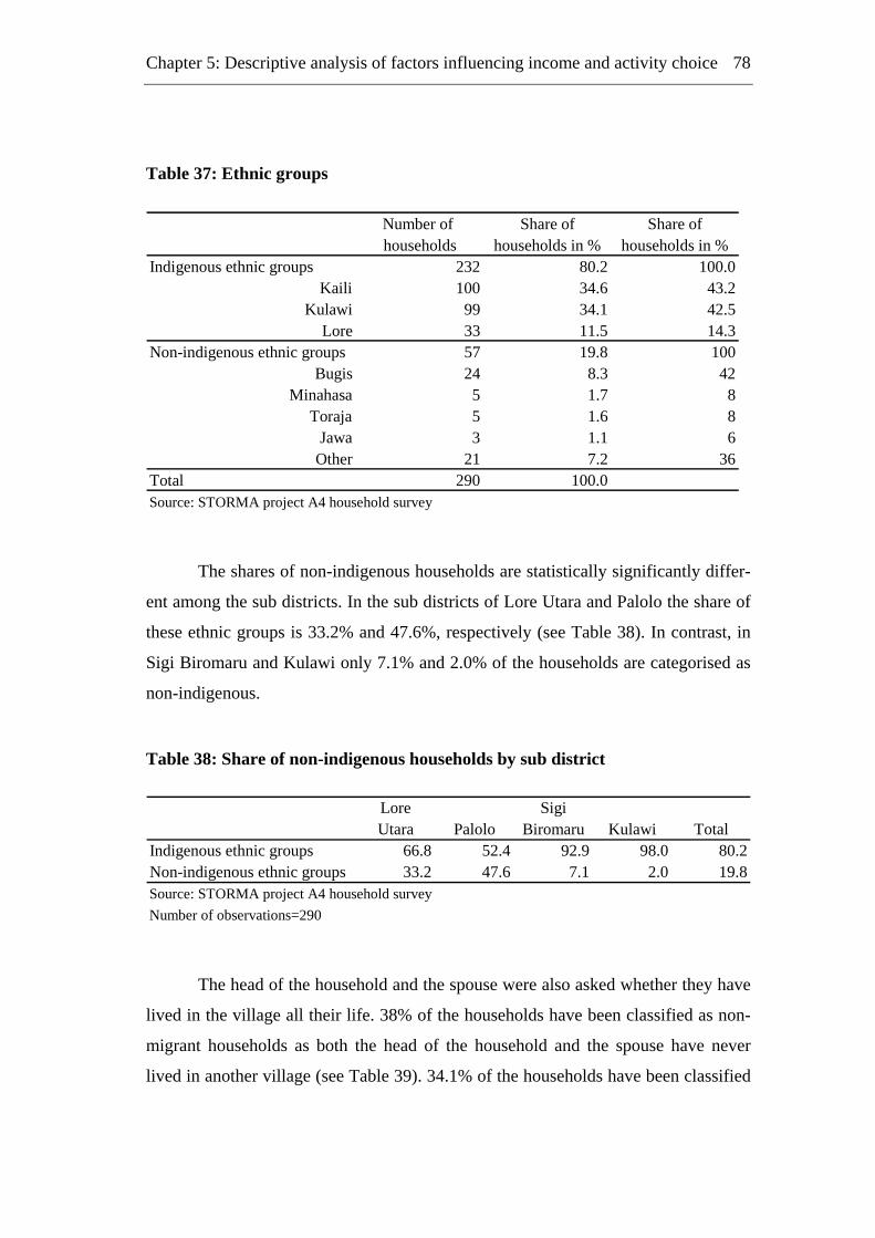
Chapter 5: Descriptive analysis of factors influencing income and activity choice
78
Table 37: Ethnic groups
Number of Share of Share of households households in % households in %
Indigenous ethnic groups 232 80.2 100.0Kaili 100 34.6 43.2
Kulawi 99 34.1 42.5Lore 33 11.5 14.3
Non-indigenous ethnic groups 57 19.8 100Bugis 24 8.3 42
Minahasa 5 1.7 8Toraja 5 1.6 8
Jawa 3 1.1 6Other 21 7.2 36
Total 290 100.0Source: STORMA project A4 household survey
The shares of non-indigenous households are statistically significantly differ-
ent among the sub districts. In the sub districts of Lore Utara and Palolo the share of
these ethnic groups is 33.2% and 47.6%, respectively (see Table 38). In contrast, in
Sigi Biromaru and Kulawi only 7.1% and 2.0% of the households are categorised as
non-indigenous.
Table 38: Share of non-indigenous households by sub district
Lore SigiUtara Palolo Biromaru Kulawi Total
Indigenous ethnic groups 66.8 52.4 92.9 98.0 80.2Non-indigenous ethnic groups 33.2 47.6 7.1 2.0 19.8Source: STORMA project A4 household surveyNumber of observations=290
The head of the household and the spouse were also asked whether they have
lived in the village all their life. 38% of the households have been classified as non-
migrant households as both the head of the household and the spouse have never
lived in another village (see Table 39). 34.1% of the households have been classified

Chapter 5: Descriptive analysis of factors influencing income and activity choice
79
as migrant households as the head of the household and the spouse used to live in a
different village. In the remaining 28% of the households, either the head of the
household or the spouse migrated into the village.
Table 39: Share of migrant households by sub district
Lore SigiUtara Palolo Biromaru Kulawi Total
Non-migrant household 31.7 4.8 38.8 73.7 38.0Migrant household 23.6 78.1 30.5 4.4 34.1Head of household only migrated in 26.8 9.5 18.8 13.9 16.9Spouse only migrated-in 17.9 7.6 11.9 7.9 11.1Source: STORMA project A4 household surveyNumber of observations=290
The share of migrant households is statistically significantly different be-
tween the sub districts. In the sub district of Kulawi 73.7% of the households are
classified as non-migrant households, whereas in Palolo 78.1% of the households are
migrant households. In the remaining sub districts migrant household also contribute
to a considerable share of the households. In the sub districts of Lore Utara and Sigi
Biromaru migrant households make up 23.6% and 30.5%, respectively. These results
are not surprising since there is a relationship between migration and ethnicity.
72.2% of the non-indigenous households are also classified as migrant households,
whereas the share in the case of the indigenous households is only 24.6%.
Concerning the migrant households, another area of concern is the year the
head of the household came to the village. More than half of migrant households
came before 1981, which shows that migration in the research area is not a new phe-
nomenon (see Table 40). Just 15% of the migrant households came in the last five
years. Among the sub districts with a considerable share of migrant households, in
Lore Utara more than one-third came in the last five years. As almost another third
came between 1991 and 1995, migration in this sub district can be regarded as a
comparably new phenomenon. In Palolo, the sub district with the highest share of
migrant households, more than 31% came in the last ten years, but 40.2% migrated
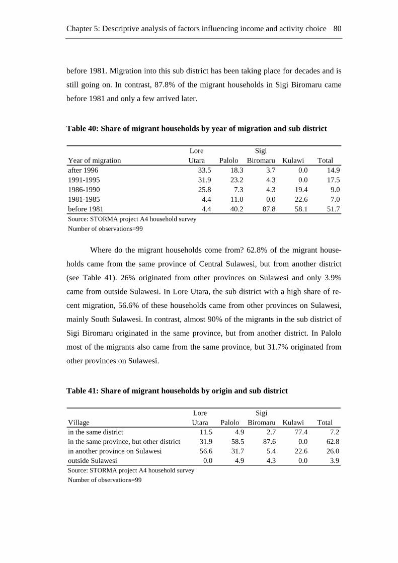
Chapter 5: Descriptive analysis of factors influencing income and activity choice
80
before 1981. Migration into this sub district has been taking place for decades and is
still going on. In contrast, 87.8% of the migrant households in Sigi Biromaru came
before 1981 and only a few arrived later.
Table 40: Share of migrant households by year of migration and sub district
Lore SigiYear of migration Utara Palolo Biromaru Kulawi Totalafter 1996 33.5 18.3 3.7 0.0 14.91991-1995 31.9 23.2 4.3 0.0 17.51986-1990 25.8 7.3 4.3 19.4 9.01981-1985 4.4 11.0 0.0 22.6 7.0before 1981 4.4 40.2 87.8 58.1 51.7Source: STORMA project A4 household surveyNumber of observations=99
Where do the migrant households come from? 62.8% of the migrant house-
holds came from the same province of Central Sulawesi, but from another district
(see Table 41). 26% originated from other provinces on Sulawesi and only 3.9%
came from outside Sulawesi. In Lore Utara, the sub district with a high share of re-
cent migration, 56.6% of these households came from other provinces on Sulawesi,
mainly South Sulawesi. In contrast, almost 90% of the migrants in the sub district of
Sigi Biromaru originated in the same province, but from another district. In Palolo
most of the migrants also came from the same province, but 31.7% originated from
other provinces on Sulawesi.
Table 41: Share of migrant households by origin and sub district
Lore SigiVillage Utara Palolo Biromaru Kulawi Totalin the same district 11.5 4.9 2.7 77.4 7.2in the same province, but other district 31.9 58.5 87.6 0.0 62.8in another province on Sulawesi 56.6 31.7 5.4 22.6 26.0outside Sulawesi 0.0 4.9 4.3 0.0 3.9Source: STORMA project A4 household surveyNumber of observations=99
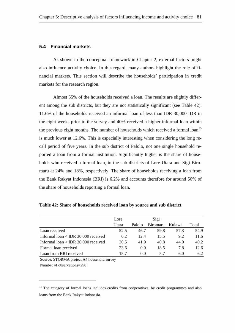
Chapter 5: Descriptive analysis of factors influencing income and activity choice
81
5.4 Financial markets
As shown in the conceptual framework in Chapter 2, external factors might
also influence activity choice. In this regard, many authors highlight the role of fi-
nancial markets. This section will describe the households’ participation in credit
markets for the research region.
Almost 55% of the households received a loan. The results are slightly differ-
ent among the sub districts, but they are not statistically significant (see Table 42).
11.6% of the households received an informal loan of less than IDR 30,000 IDR in
the eight weeks prior to the survey and 40% received a higher informal loan within
the previous eight months. The number of households which received a formal loan15
is much lower at 12.6%. This is especially interesting when considering the long re-
call period of five years. In the sub district of Palolo, not one single household re-
ported a loan from a formal institution. Significantly higher is the share of house-
holds who received a formal loan, in the sub districts of Lore Utara and Sigi Biro-
maru at 24% and 18%, respectively. The share of households receiving a loan from
the Bank Rakyat Indonesia (BRI) is 6.2% and accounts therefore for around 50% of
the share of households reporting a formal loan.
Table 42: Share of households received loan by source and sub district
Lore SigiUtara Palolo Biromaru Kulawi Total
Loan received 52.5 46.7 59.8 57.3 54.9Informal loan < IDR 30,000 received 6.2 12.4 15.5 9.2 11.6Informal loan > IDR 30,000 received 30.5 41.9 40.8 44.9 40.2Formal loan received 23.6 0.0 18.5 7.8 12.6Loan from BRI received 15.7 0.0 5.7 6.0 6.2Source: STORMA project A4 household surveyNumber of observations=290
15 The category of formal loans includes credits from cooperatives, by credit programmes and also
loans from the Bank Rakyat Indonesia.
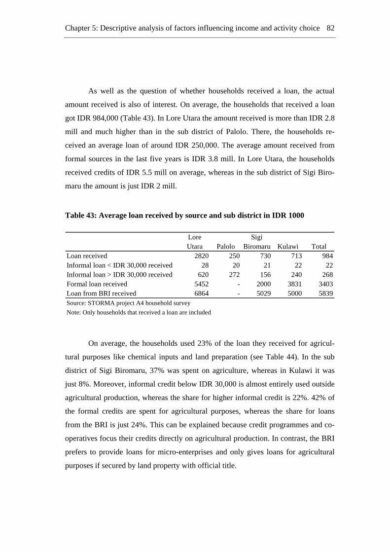
Chapter 5: Descriptive analysis of factors influencing income and activity choice
82
As well as the question of whether households received a loan, the actual
amount received is also of interest. On average, the households that received a loan
got IDR 984,000 (Table 43). In Lore Utara the amount received is more than IDR 2.8
mill and much higher than in the sub district of Palolo. There, the households re-
ceived an average loan of around IDR 250,000. The average amount received from
formal sources in the last five years is IDR 3.8 mill. In Lore Utara, the households
received credits of IDR 5.5 mill on average, whereas in the sub district of Sigi Biro-
maru the amount is just IDR 2 mill.
Table 43: Average loan received by source and sub district in IDR 1000
Lore SigiUtara Palolo Biromaru Kulawi Total
Loan received 2820 250 730 713 984Informal loan < IDR 30,000 received 28 20 21 22 22Informal loan > IDR 30,000 received 620 272 156 240 268Formal loan received 5452 - 2000 3831 3403Loan from BRI received 6864 - 5029 5000 5839Source: STORMA project A4 household surveyNote: Only households that received a loan are included
On average, the households used 23% of the loan they received for agricul-
tural purposes like chemical inputs and land preparation (see Table 44). In the sub
district of Sigi Biromaru, 37% was spent on agriculture, whereas in Kulawi it was
just 8%. Moreover, informal credit below IDR 30,000 is almost entirely used outside
agricultural production, whereas the share for higher informal credit is 22%. 42% of
the formal credits are spent for agricultural purposes, whereas the share for loans
from the BRI is just 24%. This can be explained because credit programmes and co-
operatives focus their credits directly on agricultural production. In contrast, the BRI
prefers to provide loans for micro-enterprises and only gives loans for agricultural
purposes if secured by land property with official title.
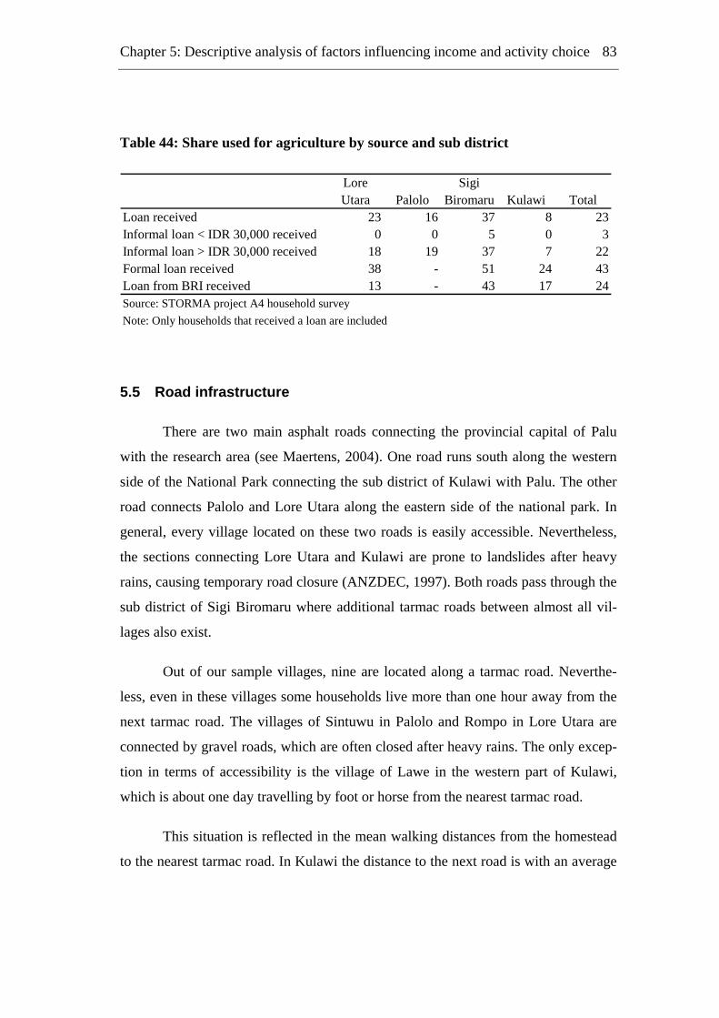
Chapter 5: Descriptive analysis of factors influencing income and activity choice
83
Table 44: Share used for agriculture by source and sub district
Lore SigiUtara Palolo Biromaru Kulawi Total
Loan received 23 16 37 8 23Informal loan < IDR 30,000 received 0 0 5 0 3Informal loan > IDR 30,000 received 18 19 37 7 22Formal loan received 38 - 51 24 43Loan from BRI received 13 - 43 17 24Source: STORMA project A4 household surveyNote: Only households that received a loan are included
5.5 Road infrastructure
There are two main asphalt roads connecting the provincial capital of Palu
with the research area (see Maertens, 2004). One road runs south along the western
side of the National Park connecting the sub district of Kulawi with Palu. The other
road connects Palolo and Lore Utara along the eastern side of the national park. In
general, every village located on these two roads is easily accessible. Nevertheless,
the sections connecting Lore Utara and Kulawi are prone to landslides after heavy
rains, causing temporary road closure (ANZDEC, 1997). Both roads pass through the
sub district of Sigi Biromaru where additional tarmac roads between almost all vil-
lages also exist.
Out of our sample villages, nine are located along a tarmac road. Neverthe-
less, even in these villages some households live more than one hour away from the
next tarmac road. The villages of Sintuwu in Palolo and Rompo in Lore Utara are
connected by gravel roads, which are often closed after heavy rains. The only excep-
tion in terms of accessibility is the village of Lawe in the western part of Kulawi,
which is about one day travelling by foot or horse from the nearest tarmac road.
This situation is reflected in the mean walking distances from the homestead
to the nearest tarmac road. In Kulawi the distance to the next road is with an average
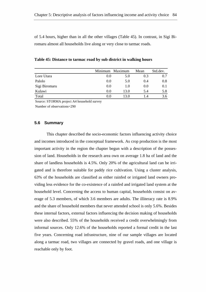
Chapter 5: Descriptive analysis of factors influencing income and activity choice
84
of 5.4 hours, higher than in all the other villages (Table 45). In contrast, in Sigi Bi-
romaru almost all households live along or very close to tarmac roads.
Table 45: Distance to tarmac road by sub district in walking hours
Minimum Maximum Mean Std.dev.Lore Utara 0.0 5.0 0.3 0.7Palolo 0.0 5.0 0.4 0.8Sigi Biromaru 0.0 1.0 0.0 0.1Kulawi 0.0 13.0 5.4 5.8Total 0.0 13.0 1.4 3.6Source: STORMA project A4 household surveyNumber of observations=290
5.6 Summary
This chapter described the socio-economic factors influencing activity choice
and incomes introduced in the conceptual framework. As crop production is the most
important activity in the region the chapter begun with a description of the posses-
sion of land. Households in the research area own on average 1.8 ha of land and the
share of landless households is 4.5%. Only 20% of the agricultural land can be irri-
gated and is therefore suitable for paddy rice cultivation. Using a cluster analysis,
63% of the households are classified as either rainfed or irrigated land owners pro-
viding less evidence for the co-existence of a rainfed and irrigated land system at the
household level. Concerning the access to human capital, households consist on av-
erage of 5.3 members, of which 3.6 members are adults. The illiteracy rate is 8.9%
and the share of household members that never attended school is only 5.6%. Besides
these internal factors, external factors influencing the decision making of households
were also described. 55% of the households received a credit overwhelmingly from
informal sources. Only 12.6% of the households reported a formal credit in the last
five years. Concerning road infrastructure, nine of our sample villages are located
along a tarmac road, two villages are connected by gravel roads, and one village is
reachable only by foot.
Chapter 5: Descriptive analysis of factors influencing income and activity choice
85
As this chapter provided a partial analysis only, the following chapter ex-
plores causal relationships by econometric modelling. It analyses the influence of the
previously described factors on total household income, activity choice and income,
and on diversification.

Chapter 6
6 Results of the econometric analysis
This chapter presents the results of the econometric models used in this thesis.
The influence of internal and external factors as described in the conceptual frame-
work on total household income, on participation in income activities as well as on
activity incomes is analysed. In the latter we consider endogeneity as well as simul-
taneity of the activity choice. In the last section, the influence of internal and external
factors on income diversification is evaluated. The following table presents the de-
scriptive statistics of all dependent variables used in the models.

Chapter 6: Results of the econometric analysis 87
Table 46: Descriptive statistics of the dependent variables
Dependent variable Min. Max. Mean Std.dev.Logarithm of total household income 10.3 17.7 14.9 1.1Participation in annual crop production 0.0 1.0 0.8 0.4Net income from annual crops (1000 IDR) -1023.0 18831.5 1181.5 1910.8Participation in perennial crop production 0.0 1.0 0.8 0.4Net income from perennial crops (1000 IDR) -1792.5 37660.1 1455.9 3881.9Participation in the sale of forest products 0.0 1.0 0.2 0.4Income from forest products (1000 IDR) 0.0 19440.0 403.4 1514.0Participation in livestock production 0.0 1.0 0.6 0.5Net-Income from livestock production (1000 IDR) -2541.2 8156.3 290.3 1002.6Participation in agric. wage labour activities 0.0 1.0 0.5 0.5Agricultural wage income (1000 IDR) 0.0 7488.0 608.9 1149.2Participation in non-agric. wage labour activities 0.0 1.0 0.2 0.4Non-agricultural wage income (1000 IDR) 0.0 21956.4 772.5 2598.1Participation in self-employment activities 0.0 1.0 0.2 0.4Net-income from non-agriculturalself-employment (1000 IDR) -90.0 36000.0 418.0 1976.9Share of non-agricultural income (%) 0.0 100.0 16.8 31.3Shannon equitibility index (%) 0.0 10000.0 8315.6 3125.8Source: Storma project A4 household surveyNumber of observations=291
In all models a common set of explanatory variables has been used to enable
comparisons of the influence of variables across models. The education of the head
of household, measured in years in school for example has been used in all models as
a proxy for education. It is now possible to compare its influence on the total house-
hold income, on participation, on activity income as well as on diversification. In
some models additional variables have been used to avoid misspecification. Theory
for example suggests that risk has an influence on diversification. Therefore, a proxy
for risk has been used in this model. Table 47 gives an overview of the descriptive
statistics of the explanatory variables used in the models.
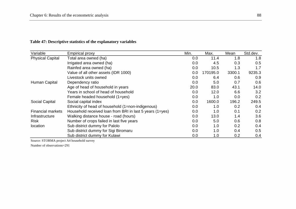
Chapter 6: Results of the econometric analysis 88
Table 47: Descriptive statistics of the explanatory variables
Variable Empirical proxy Min. Max. Mean Std.dev.Physical Capital Total area owned (ha) 0.0 11.4 1.8 1.8
Irrigated area owned (ha) 0.0 4.5 0.3 0.5Rainfed area owned (ha) 0.0 10.5 1.3 1.7Value of all other assets (IDR 1000) 0.0 170195.0 3300.1 9235.3Livestock units owned 0.0 6.4 0.6 0.9
Human Capital Dependency ratio 0.0 5.0 0.7 0.6Age of head of household in years 20.0 83.0 43.1 14.0Years in school of head of household 0.0 12.0 6.6 3.2Female headed household (1=yes) 0.0 1.0 0.0 0.2
Social Capital Social capital index 0.0 1600.0 196.2 249.5Ethnicity of head of household (1=non-indigenous) 0.0 1.0 0.2 0.4
Financial markets Household received loan from BRI in last 5 years (1=yes) 0.0 1.0 0.1 0.2Infrastructure Walking distance house - road (hours) 0.0 13.0 1.4 3.6Risk Number of crops failed in last five years 0.0 5.0 0.6 0.8location Sub district dummy for Palolo 0.0 1.0 0.2 0.4
Sub district dummy for Sigi Biromaru 0.0 1.0 0.4 0.5Sub district dummy for Kulawi 0.0 1.0 0.2 0.4
Source: STORMA project A4 household surveyNumber of observations=291
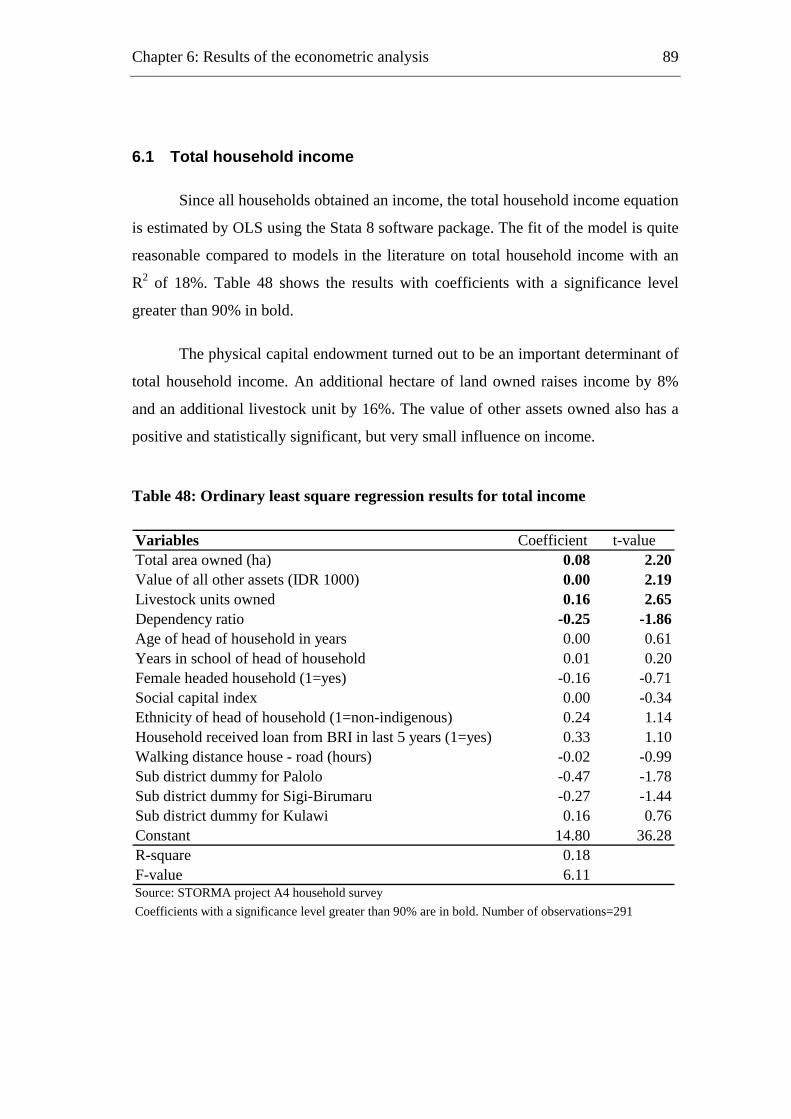
Chapter 6: Results of the econometric analysis 89
6.1 Total household income
Since all households obtained an income, the total household income equation
is estimated by OLS using the Stata 8 software package. The fit of the model is quite
reasonable compared to models in the literature on total household income with an
R2 of 18%. Table 48 shows the results with coefficients with a significance level
greater than 90% in bold.
The physical capital endowment turned out to be an important determinant of
total household income. An additional hectare of land owned raises income by 8%
and an additional livestock unit by 16%. The value of other assets owned also has a
positive and statistically significant, but very small influence on income.
Table 48: Ordinary least square regression results for total income
Variables Coefficient t-valueTotal area owned (ha) 0.08 2.20Value of all other assets (IDR 1000) 0.00 2.19Livestock units owned 0.16 2.65Dependency ratio -0.25 -1.86Age of head of household in years 0.00 0.61Years in school of head of household 0.01 0.20Female headed household (1=yes) -0.16 -0.71Social capital index 0.00 -0.34Ethnicity of head of household (1=non-indigenous) 0.24 1.14Household received loan from BRI in last 5 years (1=yes) 0.33 1.10Walking distance house - road (hours) -0.02 -0.99Sub district dummy for Palolo -0.47 -1.78Sub district dummy for Sigi-Birumaru -0.27 -1.44Sub district dummy for Kulawi 0.16 0.76Constant 14.80 36.28R-square 0.18F-value 6.11Source: STORMA project A4 household surveyCoefficients with a significance level greater than 90% are in bold. Number of observations=291
Chapter 6: Results of the econometric analysis 90
Four different empirical proxies to measure the influence of human capital
have been used. The dependency ratio, which measures the ratio of children and eld-
erly household members to adults, has a statistically significant negative influence.
This means that the more children and elderly in relation to adults are members of a
household the less the household income. An increase in the ratio by one unit in-
creases income by 25%. The influence of education is weak and not statistically sig-
nificant. An additional year spent in school by the head of the household increases
average income by 1%.
Although not statistically significant, ethnicity and participation in formal
credit markets have a strong influence on total household income. Belonging to a
non-indigenous ethnicity increases total income by 24% and borrowing from formal
sources within the last five years increased income by 33%.
The next section shifts the focus from the total income to the determinants of
participation in different activities.
6.2 Participation by activity
In the analysis of participation we differentiate seven different income
sources which are important for rural households in the research area. Non-
agricultural activities, the selling of forest products, and perennial crop production
are of special interest in terms of rural development and the overall objectives of
STORMA. The seven different binary Probit models are estimated by MLE using the
Stata 7 software package. The percentage of correctly predicted observations is on
average 78%. This value ranges from 68% correctly predicted observations in the
agricultural wage labour model to 83% in the models of annual crop production and
non-agricultural activities. Table 49 presents the regression results, with coefficients
with a significance level greater than 90% in bold. The coefficients in the table repre-
sent the percentage change in the probability for an infinitesimal change in each in-
dependent, continuous variable and the discrete change in the probability for dummy
variables. All other variables are taken at their means.
Chapter 6: Results of the econometric analysis 91
The possession of land has a strong positive influence on the participation in
crop production. An additional hectare of irrigated land increases the probability of
participation in annual crop production by 20% and in perennial crop production by
19%. The first relationship is not surprising since annual crops are grown on irrigated
as well as rainfed land. In the case of perennial crops, which are grown on rainfed
land only, the positive influence of irrigated land owned may indicate that participa-
tion in the production of perennial crops, which are mainly cash crops, requires at
least some production of rice for home consumption. The possession of irrigated land
reduces the likelihood of participation in agricultural wage labour activities, since the
production of rice is very labour intensive compared to the production of rainfed
crops. The same applies to participation in the selling of forest products. An addi-
tional hectare of irrigated land decreases the likelihood of participation in this activ-
ity by 15%. However, the possession of rainfed land increases the probability of par-
ticipation in the selling of forest products even though its influence is comparatively
weak.
The possession of other assets reduces participation in all activities except
self-employment outside agriculture. This relationship is statistically significant for
agricultural wage labour and non-agricultural self-employment income. This indi-
cates that less-poor households are more likely to participate in the latter activity,
whereas poorer households tend to participate in agricultural wage labour activities.
The possession of livestock positively influences participation in the produc-
tion of annual crops, since cattle and buffaloes are used for land preparation in paddy
rice production. However, the overall effect is not strong. An additional livestock
unit owned, which is, for example, equivalent to one buffalo, increases the likelihood
of participation by only 5%.
The education of the head of household discourages participation in the sale
of forest products, but has no statistically significant influence on the other activities.
In all activities the estimated influence of education is rather small. Holding other
variables constant, a one-year increase in the household heads’ schooling decreases
the probability of participating in the sale of forest products by only 1%.
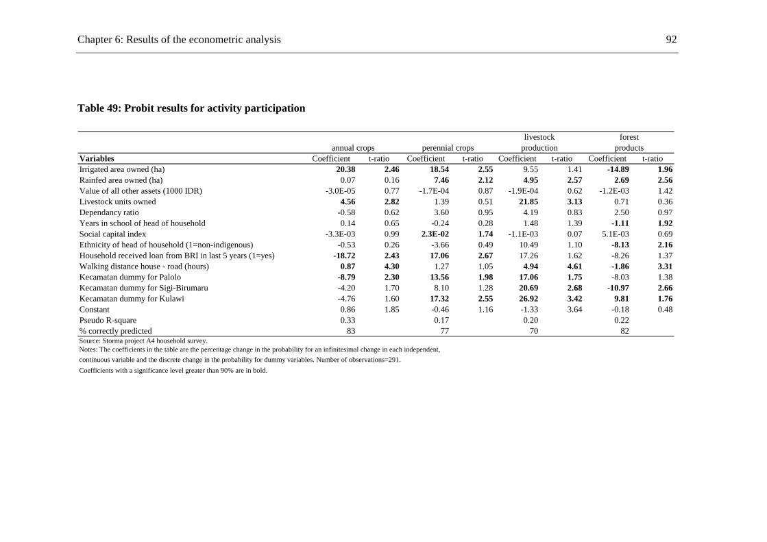
Chapter 6: Results of the econometric analysis 92
Table 49: Probit results for activity participation
Variables Coefficient t-ratio Coefficient t-ratio Coefficient t-ratio Coefficient t-ratioIrrigated area owned (ha) 20.38 2.46 18.54 2.55 9.55 1.41 -14.89 1.96Rainfed area owned (ha) 0.07 0.16 7.46 2.12 4.95 2.57 2.69 2.56Value of all other assets (1000 IDR) -3.0E-05 0.77 -1.7E-04 0.87 -1.9E-04 0.62 -1.2E-03 1.42Livestock units owned 4.56 2.82 1.39 0.51 21.85 3.13 0.71 0.36Dependancy ratio -0.58 0.62 3.60 0.95 4.19 0.83 2.50 0.97Years in school of head of household 0.14 0.65 -0.24 0.28 1.48 1.39 -1.11 1.92Social capital index -3.3E-03 0.99 2.3E-02 1.74 -1.1E-03 0.07 5.1E-03 0.69Ethnicity of head of household (1=non-indigenous) -0.53 0.26 -3.66 0.49 10.49 1.10 -8.13 2.16Household received loan from BRI in last 5 years (1=yes) -18.72 2.43 17.06 2.67 17.26 1.62 -8.26 1.37Walking distance house - road (hours) 0.87 4.30 1.27 1.05 4.94 4.61 -1.86 3.31Kecamatan dummy for Palolo -8.79 2.30 13.56 1.98 17.06 1.75 -8.03 1.38Kecamatan dummy for Sigi-Birumaru -4.20 1.70 8.10 1.28 20.69 2.68 -10.97 2.66Kecamatan dummy for Kulawi -4.76 1.60 17.32 2.55 26.92 3.42 9.81 1.76Constant 0.86 1.85 -0.46 1.16 -1.33 3.64 -0.18 0.48Pseudo R-square 0.33 0.17 0.20 0.22% correctly predicted 83 77 70 82Source: Storma project A4 household survey.Notes: The coefficients in the table are the percentage change in the probability for an infinitesimal change in each independent,continuous variable and the discrete change in the probability for dummy variables. Number of observations=291.Coefficients with a significance level greater than 90% are in bold.
annual crops perennial crops productionforest
productslivestock
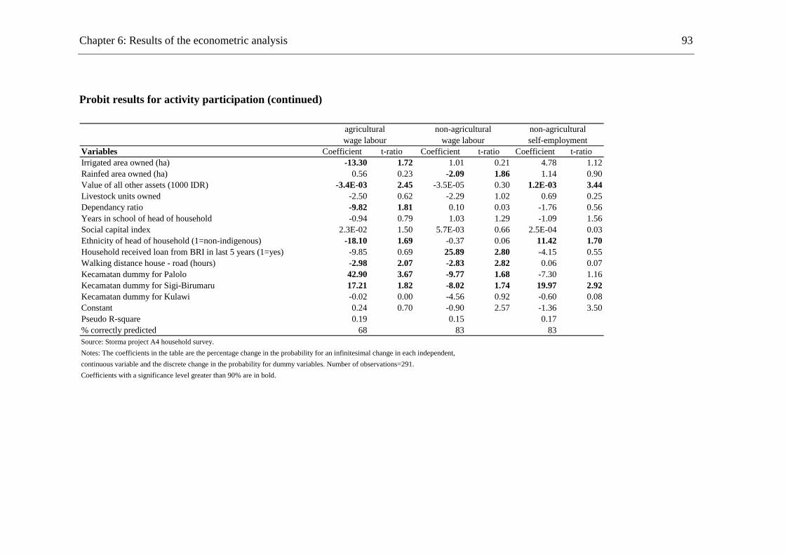
Chapter 6: Results of the econometric analysis 93
Probit results for activity participation (continued)
Variables Coefficient t-ratio Coefficient t-ratio Coefficient t-ratioIrrigated area owned (ha) -13.30 1.72 1.01 0.21 4.78 1.12Rainfed area owned (ha) 0.56 0.23 -2.09 1.86 1.14 0.90Value of all other assets (1000 IDR) -3.4E-03 2.45 -3.5E-05 0.30 1.2E-03 3.44Livestock units owned -2.50 0.62 -2.29 1.02 0.69 0.25Dependancy ratio -9.82 1.81 0.10 0.03 -1.76 0.56Years in school of head of household -0.94 0.79 1.03 1.29 -1.09 1.56Social capital index 2.3E-02 1.50 5.7E-03 0.66 2.5E-04 0.03Ethnicity of head of household (1=non-indigenous) -18.10 1.69 -0.37 0.06 11.42 1.70Household received loan from BRI in last 5 years (1=yes) -9.85 0.69 25.89 2.80 -4.15 0.55Walking distance house - road (hours) -2.98 2.07 -2.83 2.82 0.06 0.07Kecamatan dummy for Palolo 42.90 3.67 -9.77 1.68 -7.30 1.16Kecamatan dummy for Sigi-Birumaru 17.21 1.82 -8.02 1.74 19.97 2.92Kecamatan dummy for Kulawi -0.02 0.00 -4.56 0.92 -0.60 0.08Constant 0.24 0.70 -0.90 2.57 -1.36 3.50Pseudo R-square 0.19 0.15 0.17% correctly predicted 68 83 83Source: Storma project A4 household survey.Notes: The coefficients in the table are the percentage change in the probability for an infinitesimal change in each independent,continuous variable and the discrete change in the probability for dummy variables. Number of observations=291.Coefficients with a significance level greater than 90% are in bold.
wage labour wage labour self-employmentagricultural non-agricultural non-agricultural
Chapter 6: Results of the econometric analysis 94
Social capital leads to increased participation in the production of perennial
crops, but has no statistically significant influence on the other activities. A reason
for this might be that cacao, the most important perennial crop, is a comparatively
new crop for the farmers in the research area. More than two-thirds of the cocoa plots
are less than 5 years old. Farmers often get to know of a new crop by the experiences
of other farmers. Moreover, other farmers are often the most-trusted and only source
of information on how to start the cultivation. Meetings of social organisations are a
good opportunity to meet other farmers and discuss such issues. The econometric
analysis seems to reveal the importance of social capital in the adoption process of a
new crop.
Indigenous households tend to participate in agricultural wage labour and in
the selling of forest products, whereas non-indigenous households are more likely to
participate in non-agricultural self-employment. Belonging to a non-indigenous eth-
nic group decreases the probability of participation in the sale of forest products by
8% and in agricultural wage labour activities by 18%. On the other hand, it increases
the likelihood of participation in non-agricultural self-employment by 11%. All three
relationships are statistically significant.
Borrowing money from the BRI plays an interesting role in determining ac-
tivity participation. It statistically significantly discourages participation in annual
crop production, but encourages participation in the production of perennial crops
and non-agricultural wage labour. The latter influence is particularly strong, increas-
ing the probability of participation by 26%. When a household received a loan in the
last five years the probability of participating in annual crop production decreased by
around 19%, whereas the likelihood of participating in perennial crop production
increased by 17%. This result suggests that formal loans are used to start the produc-
tion of perennial crops, mainly cocoa, and therefore might accelerate the conversion
of forest into cocoa plantations.
Infrastructure, measured by the walking distance to the next road, has a strong
influence on participation in almost all activities. The longer a household needs to
get to the next road, the more likely it will participate in crop and livestock produc-
Chapter 6: Results of the econometric analysis 95
tion. This relationship is statistically significant in the case of annual crop production
and livestock production. Every hour further away from a tarmac road increases the
likelihood to participate in annual crop production by 1%. On the other hand, in-
creasing distance reduces the likelihood of participating in wage labour activities and
in the selling of forest products. The latter result is somewhat surprising because in
general, forest products are associated with remote areas. This could be due to the
fact that we only considered the selling of forest products, and the sale of rattan re-
quires good road infrastructure. With every hour of increasing distance to the road
the probability of participating in non-agricultural wage labour employment de-
creases by almost 3%. The only exception in the influence of roads is non-
agricultural self-employment, where the coefficient and the t-ratio are very low, indi-
cating that it has no influence on participation. In line with the descriptive results,
this reflects the fact that the rural non-agricultural self-employment sector is domi-
nated by small enterprises serving local markets independent of the existence of tar-
mac roads.
Finally, a number of regional variables turned out to statistically significantly
influence participation in particular activities, which indicates the existence of certain
regional factors that are not controlled for in the regression models.
6.3 Income by activity
While the previous section evaluated the probability of participation in activi-
ties, this section analyses factors influencing the level of income from each activity.
The same income activities as before are used with the same set of explanatory vari-
ables, but only those physical assets that are expected to influence the income level
of a certain activity are included. The income equations are estimated jointly, apply-
ing a generalisation of the Lee two-stage estimator proposed by Amemiya as de-
scribed in Chapter 3. The Limdep 7.0 software package was used for estimation. The
fit of the models measured by the R-square ranges from 60% to 80%. Table 50 pre-
sents the regression results, with coefficients with a significance level greater than
90% in bold. The coefficients in the table are the estimated absolute effects of one-
Chapter 6: Results of the econometric analysis 96
unit changes in the corresponding explanatory variables on activity incomes. They
represent effects of explanatory variables on activity incomes given participation and
thus are also called selectivity-corrected activity income estimates.
As expected the area of land owned plays an important role not only in crop
production, but also in the selling of forest products and in wage labour activities. An
additional hectare of irrigated land increases income from annual crop production by
IDR 399,000 IDR, which is equivalent to 34%. The area of rainfed land owned has
almost the same effect on income from perennial crops controlled for participation.
The absolute gain in income from perennial crops is IDR 680,000 or 47%. Besides
its influence on annual crop production, irrigated land also has a strong influence on
the income from forest products and agricultural wage labour. Each additional hec-
tare owned decreases income from the sale of forest products by IDR 356,000, which
is equivalent to a reduction of 88%. Furthermore, an additional hectare of irrigated
land reduces income from agricultural wage labour by IDR 248,000. Thus, the very
labour intensive production of paddy rice not only reduces the likelihood of partici-
pation, it also reduces the income gained from these activities. Moreover, the results
indicate that the ownership of land reduces the income gained from wage labour ac-
tivities in general.
In contrast to land, the effect of the value of other assets owned on activity
incomes is small, and with the exception of non-agricultural self-employment income
not statistically significant. This result is not surprising because the category other
assets also includes non-productive assets, like radios and televisions, which are not
used in the production process.
The possession of livestock leads not only to increased participation in annual
crop production and livestock production, but also positively influences income
gained from these activities. Both relationships are statistically significant.
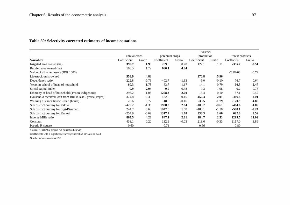
Chapter 6: Results of the econometric analysis 97
Table 50: Selectivity corrected estimates of income equations
Variables Coefficient t-ratio Coefficient t-ratio Coefficient t-ratio Coefficient t-ratioIrrigated area owned (ha) 399.7 1.93 289.8 0.70 122.1 1.11 -355.7 -2.51Rainfed area owned (ha) 108.5 1.72 680.1 4.84Value of all other assets (IDR 1000) -2.9E-03 -0.72Livestock units owned 559.9 4.83 370.8 5.96Dependency ratio -222.8 -0.76 -402.7 -1.13 -9.0 -0.10 76.7 0.64Years in school of head of household 60.3 1.79 -83.7 -1.17 14.1 0.79 -60.3 -2.47Social capital index 0.9 2.04 -0.2 -0.38 0.3 1.08 0.2 0.73Ethnicity of head of household (1=non-indigenous) 298.2 1.08 1208.3 2.00 15.4 0.10 -87.1 -0.42Household received loan from BRI in last 5 years (1=yes) 374.8 0.35 182.5 0.15 456.3 2.01 -319.4 -1.01Walking distance house - road (hours) 28.6 0.77 -18.0 -0.16 -33.5 -1.79 -120.9 -4.80Sub district dummy for Palolo -429.2 -1.36 1988.8 2.84 -108.2 -0.61 -464.6 -1.89Sub district dummy for Sigi-Birumaru 244.7 0.63 1047.5 1.60 -180.1 -1.10 -508.1 -2.24Sub district dummy for Kulawi -254.9 -0.69 1317.7 1.70 338.3 1.66 692.0 2.52Inverse Mills ratio 863.5 4.23 847.1 2.81 184.7 2.53 1299.5 11.09Constant 438.1 0.20 132.6 -0.03 218.6 -0.33 1157.0 3.89Pseudo R-square 0.60 0.71 0.66 0.80Source: STORMA project A4 household surveyCoefficients with a significance level greater than 90% are in bold.Number of observations=291
annual crops perennial crops forest productslivestock
production
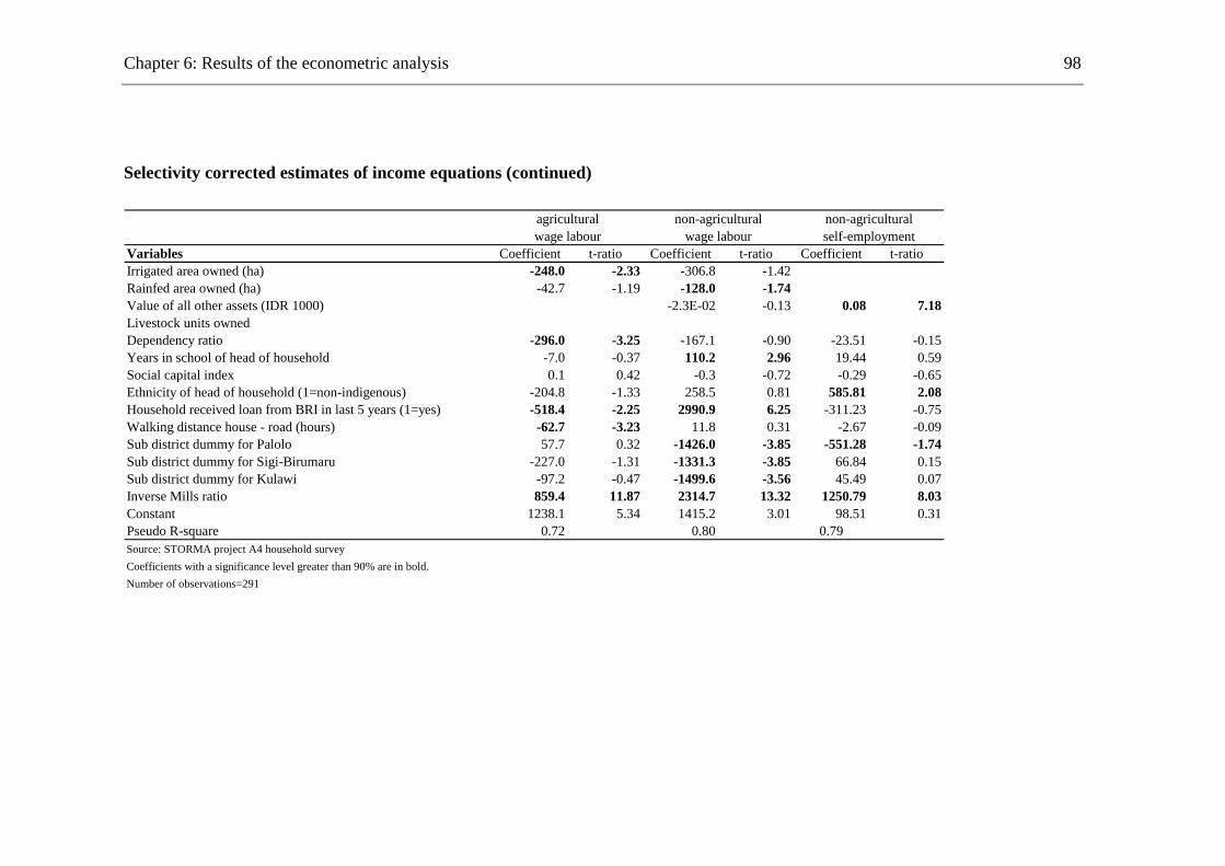
Chapter 6: Results of the econometric analysis 98
Selectivity corrected estimates of income equations (continued)
Variables Coefficient t-ratio Coefficient t-ratio Coefficient t-ratioIrrigated area owned (ha) -248.0 -2.33 -306.8 -1.42Rainfed area owned (ha) -42.7 -1.19 -128.0 -1.74Value of all other assets (IDR 1000) -2.3E-02 -0.13 0.08 7.18Livestock units ownedDependency ratio -296.0 -3.25 -167.1 -0.90 -23.51 -0.15Years in school of head of household -7.0 -0.37 110.2 2.96 19.44 0.59Social capital index 0.1 0.42 -0.3 -0.72 -0.29 -0.65Ethnicity of head of household (1=non-indigenous) -204.8 -1.33 258.5 0.81 585.81 2.08Household received loan from BRI in last 5 years (1=yes) -518.4 -2.25 2990.9 6.25 -311.23 -0.75Walking distance house - road (hours) -62.7 -3.23 11.8 0.31 -2.67 -0.09Sub district dummy for Palolo 57.7 0.32 -1426.0 -3.85 -551.28 -1.74Sub district dummy for Sigi-Birumaru -227.0 -1.31 -1331.3 -3.85 66.84 0.15Sub district dummy for Kulawi -97.2 -0.47 -1499.6 -3.56 45.49 0.07Inverse Mills ratio 859.4 11.87 2314.7 13.32 1250.79 8.03Constant 1238.1 5.34 1415.2 3.01 98.51 0.31Pseudo R-square 0.72 0.80 0.79Source: STORMA project A4 household surveyCoefficients with a significance level greater than 90% are in bold.Number of observations=291
non-agriculturalself-employmentwage labour
agricultural non-agriculturalwage labour
Chapter 6: Results of the econometric analysis 99
Education plays an interesting role as a determinant of activity income. A
one-year increase in household heads’ schooling increases income from annual crop
production by IDR 60,000, which is equivalent to a return of 5%. On the other hand,
it reduces the gains from the production of perennial crops, although this influence is
not statistically significant. As formal education influences management practices
this result indicates that management issues are important for the production of an-
nual crops, whereas they do not play such a role in perennial crop production. This is
in line with the descriptive analysis in Chapter 4.2.1, which shows that 81% of the
cash expenditures for inputs are spent for annual crops, especially paddy rice. Formal
education, especially the ability to read and write, is important in the use of chemical
inputs, for example to read the description and dosage recommendations on the tins
of pesticides. Furthermore, an additional year in school reduces the income gained
from the selling of forest products by IDR 60,000, which is equivalent to a reduction
of 15%. The highest returns of education are gained in non-agricultural wage labour
income. A one-year increase in household heads’ schooling is associated with an
absolute gain of IDR 110,000, which is equivalent to an increase in non-agricultural
wage labour income by 14%. This is in line with findings of similar studies on the
role of education from Latin America (Taylor and Yunez-Naude, 2000, Yunez-
Naude and Taylor, 2001, Winters et al., 2002). Taylor and Yunez-Naude (2000), for
example, report returns of education of 10% to wage labour income.
Social capital has a positive influence on the incomes gained from annual
crop production, but has no statistically significant influence on the other activities.
The influence of social capital on annual crop production might be explained by the
importance of external inputs in its production. Meetings of social organisations are
a good opportunity to meet other farmers and discuss the use of chemical fertiliser
and pesticides, especially when other sources of information, like the extension ser-
vice, are often not available.
Ethnic affiliation has a strong and statistically significant effect on income
from perennial crop production and non-agricultural self-employment. Although
non-indigenous households are less likely to participate in the production of peren-
Chapter 6: Results of the econometric analysis 100
nial crops, they gain almost IDR 1.2 mill, which is equivalent to an increase of 83%.
In non-agricultural self-employment, ethnicity also has a statistically significant in-
fluence, with non-indigenous households gaining IDR 585,000 compared to indige-
nous households.
Participation in formal credit markets has a positive and statistically signifi-
cant influence on income from livestock production, and both agricultural and non-
agricultural wage labour activities. The latter relationship is particularly strong. This
might be explained by a change in causality: for households having a high and regu-
lar wage income it is much easier to get loans from formal institutions.
The distance to the next road has a statistically significant influence on in-
come from livestock production, agricultural wage labour activities and the selling of
forest products. The latter relationship is particularly strong. With every hour of in-
creased distance to the road, the income from forest products decreases by around
IDR 120,000, which is equivalent to a drop of 30%. In this activity, distance to roads
has the same strong and statistically significant influence on both participation and
income. Similar but less strong is the impact of infrastructure on agricultural wage
labour income. The influence of roads on income from activities outside the agricul-
tural sector is low and statistically not significant.
In all equations the estimates for the IMR are all positive and statistically sig-
nificantly different from zero, which indicates that self-selection into activities plays
an important role in the generation of income from a certain activity. Moreover, the
failure to control for it would have led to biased results.
6.4 Diversification
The term income diversification is often used in the sense of diversification out
of the agricultural sector, i.e. as an increase in the share of income from activities
which are not related to agriculture. This is examined in the first econometric model,
where we look at factors influencing diversification out of the agricultural sector. It
is measured by the share of non-agricultural income, both from self-employment and
Chapter 6: Results of the econometric analysis 101
wage labour, in total household income. But income diversification can also refer to
the number of income sources and their relative importance. This is examined in the
second model, where we analyse the factors influencing the overall mix of the in-
come measured by the Shannon equitability index. This index takes into account the
number of income sources and their share in total household income. It increases
with the number of income sources and when the income is more evenly distributed
among the different activities. It is calculated from the same activities as considered
in the previous sections (for computational details see Chapter 3.3.2). In both regres-
sions we use the same set of explanatory variables whose descriptive statistics are
shown in Table 47.
In the first regression on the share of non-agricultural income in total house-
hold income the value of other assets owned has a highly statistically significant
positive influence (see Table 51). Wealth increases the diversification out of the agri-
cultural sector. Another statistically significant factor influencing the diversification
out of agriculture is education. The more years the head of the household spent in
school, the greater the household’s share in non-agricultural income. Also, participa-
tion in formal credit markets has a statistically significant positive impact on the
share of non-agricultural income.
Considering the overall degree of diversification, the possession of land and
of other assets has no statistically significant influence on the Shannon equitability
index, whereas the number of livestock owned by a household increases the overall
diversity of income. Social networks also seem to enable household members to ex-
tend their participation to new activities. Social capital has a statistically significant
and positive influence on diversification. Despite being statistically not significant,
the occurrence of shocks related to cropping activities within the last 10 years posi-
tively influences the overall diversification. This supports the hypothesis of diversifi-
cation as an ex-post reaction to the occurrence of shocks.

Chapter 6: Results of the econometric analysis 102
Table 51: Tobit estimates of the determinants of diversification
Variables Coefficient t-ratio Coefficient t-ratioTotal area owned (ha) -1.60 -0.55 1.07E-02 1.56Value of all other assets (IDR 1000) 8.4E-04 2.31 4.03E-08 0.03Livestock units owned -1.12 -0.22 3.11E-02 2.52Dependency ratio -3.80 -0.47 -1.16E-03 -0.06Years in school of head of household 2.66 1.65 -5.71E-03 -1.52Social capital index -5.8E-03 -0.29 1.07E-04 2.21Female headed household (1=yes) 34.41 1.43 6.50E-02 1.10Ethnicity of head of household (1=non-indigenous) 15.23 1.16 -2.90E-02 -0.91Household received loan from BRI in last 5 years (1=yes) 50.29 3.07 -3.70E-03 -0.08Walking distance house - road (hours) -0.64 -0.26 1.11E-03 0.28Number of crops failed in last five years -4.68 -0.75 1.92E-02 1.39Sub district dummy for Palolo -30.82 -1.82 2.40E-02 0.64Sub district dummy for Sigi-Birumaru 8.54 0.64 1.97E-02 0.55Sub district dummy for Kulawi -39.40 -2.39 1.31E-01 3.01Constant -34.96 -1.76 2.73E-01 5.70Prob. > Chi-square 0.00 0.00Number of left censored observations 190 32Source: STORMA project A4 household survey.Notes: The coefficients show the marginal effect of the explanatory variables on the latent variable.Coefficients with a significance level greater than 90% are in bold. Number of observations=291
non-agricultural income equitibility indexShare of Shannon

Chapter 6: Results of the econometric analysis 103
Comparing the two models we can conclude that the households’ wealth posi-
tively influences diversification out of the agricultural sector, whereas it has no influ-
ence on the overall income diversity. The same applies for the role of participation in
formal credit markets. Furthermore, education plays a major positive role in the di-
versification out of the agricultural sector but it has a negative influence on the over-
all diversification. Better-educated households have a higher share of income from
outside agriculture, but their income stems from fewer sources and is less evenly
distributed among these sources.
6.5 Summary
This chapter presented the results of the econometric models used in this the-
sis. The access to physical and human capital has a significant influence on total
household income. The area owned, the value of other assets possessed, as well as
the number of livestock and family labourers positively influence total household
income. The analysis of activity choice shows the strong influence of the possession
of land on the participation in crop production, while the possession of irrigated land
reduces the likelihood of participation in agricultural wage labour activities and in
the sale of forest products. Richer and non-indigenous households are more likely to
participate in non-agricultural self-employment. In contrast, non-indigenous house-
holds are less likely to participate in the sale of forest products and in agricultural
wage labour activities. Participation in formal credit markets discourages participa-
tion in annual crop production, but encourages participation in the production of per-
ennial crops and non-agricultural wage labour activities. The access to roads has a
strong influence on participation in almost all activities. The analysis of activity in-
comes shows that the possession of land has a strong positive influence on the in-
come gained from crop production, while the possession of irrigated land reduces the
income gained from agricultural wage labour and the sale of forest products. Similar
to its effect on participation, the value of other assets owned has a positive influence
on the income from non-agricultural self-employment. Furthermore, the analysis
shows that education increases the income gained from non-agricultural wage labour
activities and annual crop production. Compared to indigenous households, non-
Chapter 6: Results of the econometric analysis 104
indigenous households gain more income from perennial crop production and non-
agricultural self-employment. The access to tarmac roads has a positive effect on the
income from agricultural wage labour and the sale of forest products. Diversification
out of the agricultural sector is positively influenced by the wealth of the household,
education, and the participation in formal credit markets.
The next chapter summarises the major results related to the research ques-
tions presented in Chapter 2.
Chapter 7
7 Conclusions
The research area is characterised by a high share of poor and vulnerable
households (Suryahadi and Sumarto, 2001) as well as by a strong increase in popula-
tion. These people were and are attracted by the income possibilities in coffee and
particularly in cocoa production, which is a major source of deforestation and often
located inside the Lore-Lindu National Park (Maertens, 2003). This ongoing en-
croachment threatens the integrity of the park and endangers its unique fauna and
flora. Therefore, alternative income sources for rural households are needed which
are able to reduce poverty and the pressure on the national park. This study aims to
identify and analyse the determinants of income generating activities of rural house-
holds in the vicinity of the national park. It helps to identify factors, which are essen-
tially for the design of policies promoting alternative income strategies.
This chapter summarises the major results related to the research questions
presented in Chapter 2. The first section presents the results related to the research
questions 1 through 6 and the final section draws policy conclusions in relation to
research question 7.
Conclusions 106
7.1 Major results
Among the activities in which rural households in the research area are en-
gaged, agricultural activities are the most important source of income. They account
for 70% of the total household income, with 96% of the households participating in
this activity. Within this category, most income originates from crop production,
with cocoa and paddy rice as the most important crops. Nevertheless, activities out-
side the agricultural sector also play an important role and contribute 30% to the total
income. Compared to this share, participation in non-agricultural activities is much
lower. Only 17% of the households generate income from non-agricultural wage
labour activities and 18% from non-agricultural self-employment.
Differentiating the income sources by poverty groups show differences be-
tween poor and less-poor households in their activities. Participation in agricultural
wage labour activities is much lower for less-poor households compared to the poor-
est households. In contrast, the rate of participation in non-agricultural activities is
comparatively higher for households that are better off. Moreover, they generate also
much more income from these activities. They derive 39% of their income from ac-
tivities outside agriculture, whereas it accounts for only 9% of the income of the
poorest households.
The econometric analysis shows that the access to physical and human capital
has a significant influence on total household income. The size of land owned, the
value of other assets possessed, and the number of livestock owned have a positive
influence on total household income. Furthermore, the dependency ratio has a nega-
tive influence. This means that the more members of working age in relation to chil-
dren and elderly are in a household, the higher the household income.
Another area of concern in the econometric analysis is the examination of
factors determining participation in different activities. The possession of land, social
capital and the participation in formal credit markets have a positive influence on the
participation in perennial crop production. The level of schooling and the distance to
tarmac roads decrease the probability of participating in the sale of forest products.
Moreover, non-indigenous households are less likely to participate in this activity. It
Conclusions 107
is also interesting to note that the possession of irrigated land reduces the likelihood
of participation, whereas the area of rainfed land owned has a positive influence on
participation in the sale of forest products. Participation in formal credit markets has
a positive influence on the participation in non-agricultural wage labour activities,
whereas the area of irrigated land owned and the distance to a tarmac road discour-
ages participation in this activity. The value of other assets owned increase the prob-
ability of participating in non-agricultural self-employment. Moreover, non-
indigenous households are more likely to participate in this activity.
Apart from participation in activities, another econometric model analyses
factors influencing the income gained from different activities. As in the case of par-
ticipation, the possession of rainfed land also has a strong positive influence on the
income gained from perennial crop production. Moreover, non-indigenous house-
holds gain more income from perennial crop production than indigenous households.
The possession of irrigated land, the level of education and the distance to a tarmac
road reduce the income gained from the sale of forest products. The analysis also
shows that education increases the income gained from non-agricultural wage labour
activities. In contrast, the area owned has a negative influence on the income from
that activity. Similar to its effect on participation, the value of other assets has a posi-
tive influence on the income from non-agricultural self-employment. Furthermore,
non-indigenous households gain more income from that activity than indigenous
households.
The final econometric model examines factors influencing income diversifi-
cation. The diversification out of the agricultural sector is positively influenced by
the wealth status of the household, the education of the head of household, and the
participation in formal credit markets. The number of livestock owned and the access
to social capital have a positive effect on the overall degree of diversification.
7.2 Policy conclusions
Based on the results of the descriptive as well as econometric analysis, policy
conclusions can be drawn with respect to deforestation and rural development. The
Conclusions 108
latter topic focuses on poverty alleviation through the promotion of activities outside
the agricultural sector.
An important area of concern is the income derived from perennial crops, as
coffee and cocoa are a major source of deforestation. The econometric analysis
shows that the possession of land, the access to social capital and the participation in
credit markets positively influences participation in perennial crop production. The
positive influence of the possession of irrigated land on participation in perennial
crop production may indicate a food security strategy employed by rural households.
Irrigated land for the production of the basic staple rice seems to be a prerequisite for
participation in perennial crop production. But the area of irrigated land owned has
no statistically significant effect on the income derived. The positive influence of
borrowing money from the BRI on participation suggests that such loans are used to
start the production of perennial crops, which accelerate the conversion of forest into
cocoa plantations. Therefore, formal credits should be redirected into activities which
do not threaten the integrity of the national park. Alternatives might include non-
agricultural activities, which are constrained by the access to formal credit. Neverthe-
less, all such policies aiming to protect the park should be accompanied by better law
enforcement either through the National Park Authority or community agreements16.
Apart from deforestation, another area of concern is the sale of forest prod-
ucts, which are mainly collected inside the national park. The level of education and
the distance to tarmac roads have a negative influence on the sale of forest products.
Therefore, policy measures to reduce the sale of forest products might be to improve
the access to education and rethink the proposed road extension plans. In the political
discussion, there are still plans to build new roads inside the national park linking,
for example, the sub district of Lure Utara with Lore Selatan (ANZDEC, 1997). Al-
ternative plans building these roads further away from the national park boundaries
should be preferred.
16 The effect of various community agreements on conservation in the research area has been evalu-
ated in Mappatoba, 2004

Conclusions 109
The analysis was designed to enable a thorough investigation of non-
agricultural activities, as these might represent a way out of poverty without leading
to further deforestation. The descriptive analysis shows that non-agricultural activi-
ties are particularly important for less-poor households, whereas poor households are
more engaged in agricultural activities. Reardon et al. (1998) call this the “inter-
household paradox”: the poorest households, while having the greatest need for non-
agricultural income, are also the most constrained. The econometric analysis shows
that the endowment of other assets is such a constrain. Poorer households, because of
their lower endowment with physical capital not related to agriculture, have fewer
opportunities to participate and derive income from non-agricultural sources. There-
fore, potential non-agricultural activities have to be carefully evaluated as to whether
they suit the assets owned by poor households. Agricultural policies or projects aim-
ing to reduce poverty by promoting these activities have to consider this. Otherwise,
they will not be able to participate and it will not be possible to reduce poverty by
promoting non-agricultural activities.
Apart from the value of other assets owned, another key determinant for in-
come diversification out of the agricultural sector is the participation in formal credit
markets. Households that have received a formal loan within the last five years have
diversified more of their income out of the agricultural sector than households that
did not receive a formal loan. Credit enables households to change their stock in
physical capital within a short time to take advantage of income opportunities outside
agriculture. Therefore, a possible policy measure is to improve the participation of
poor households in formal credit, which are directly targeted towards non-
agricultural activities.
Another key factor influencing income from non-agricultural wage labour
with high returns is education. A one-year increase in household heads’ schooling is
associated with an increase in non-agricultural wage labour income by 14%. The
improvement of the level of education, especially of junior and senior high schools,
is a prerequisite for wage labour employment outside the agricultural sector. There-
fore, rural development policies could promote the establishment of additional junior
Conclusions 110
and senior high schools. But, the demand for better-educated people also has to be
improved, especially in the private sector. So far, the state is the most important em-
ployer and governmental budgets are tight.
Activities outside the agricultural sector represent an alternative income sour-
ce without leading to further encroachment. Nevertheless, the descriptive as well as
econometric analysis indicate that self-employed income is dominated by small en-
terprises serving local markets, implying linkages between the agricultural and non-
agricultural sector. The business of small shopkeepers and craftsmen in the villages
depends on the economic situation of the farmers in their village. Changing the focus
of rural development programmes from the agricultural to the non-agricultural sector
might create new activities in the villages outside agriculture, but it can also decrease
the demand of local farmers to the disadvantage of already existing local shops and
craftsmen. Such dependencies call for multisectoral development policies taking into
account the multiplicity of activities and their inter-linkages. Reardon et al. (2001, p.
407), in an overview of policy implications for rural non-farm employment in Latin
America, drew the conclusions that “the promotion of rural non-agricultural em-
ployment and income cannot be made at the cost of developing the agricultural sec-
tor. The challenge consists of mobilizing additional investment […].”
8 References
Abu Shaban, A. 2001. Rural Poverty and Poverty outreach of Social Safety Net pro-grams in Central Sulawesi - Indonesia. MSc- thesis, Institute of Rural Devel-opment, University of Göttingen.
Amemiya, T. 1977. The estimation of a simultaneous-equation tobit model. Stanford University, Institute for Mathematical Studies in the Social Sciences, Techni-cal Report 236.
ANZDEC. 1997. Report on the Central Sulawesi integrated area development and conservation project. Palu, Sulawesi, Indonesia.
Asra, A. 2000. Poverty and inequality in Indonesia : estimates, decomposition and key issues. In: Journal of the Asia Pacific economy 5 (1/2): 91-111.
Barrett, C. B. and Reardon, T. 2000. Asset, Activity, Income Diversification Among African Agriculturists: Some Practical Issues. Project report to the USAID BASIS CRSP.
Barrett, C. B., Reardon, T. and Webb, P. 2001. Nonfarm income diversification and household livelihood strategies in rural Africa: concepts, dynamics, and pol-icy implications. In: Food Policy 26 (2001): 315-331.
References 112
Belsley, D. A., Kuh, E. and Welsch, R. 1980. Regression diagnostics: identifying influential data and sources. New York: Wiley.
Black, T. R. 1999. Doing quantitative research in the social sciences : an integrated approach to research design, measurement and statistics. London: SAGE Pub-lications.
Burns, R. S. 2000. Introduction to Research Methods. London: Sage Publications.
Canagarajah, S., Newman, C., Bhattamishra, R. 2001. Non-farm income, gender, and inequality: evidence from rural Ghana and Uganda. In: Food Policy 26 405-420.
Chambers, R. and Conway, G. R. 1992. Sustainable rural livelihoods : practical con-cepts for the 21st century. Brighton: Institute of Development Studies.
Collier, P. 1998. Social Capital and Poverty. Social Capital Initiative Working Paper No.4. Washington, D.C.: World Bank.
Corral, L. and Reardon, T. 2001. Rural Nonfarm Incomes in Nicaragua. In: World Development 29 (3): 427-442.
de Janvry, A., and E. Sadoulet. 2001. Income Strategies Among Rural Households in Mexico: The Role of Off-farm Activities. In: World Development 29 (3): 467-480.
de Janvry, A., Fafchamps,M., and E. Sadoulet. 1991. Peasant Household Behaviour with Missing Markets: Some Paradoxes Explained. In: Economic Journal 101 1400-1417.
de Janvry, A., Sadoulet, E. and Murgai, R. 2002. Rural development and rural policy. In: B. L. Gardner and G. C. Rausser (ed.). Handbook of agricultural econom-ics. 1593-1658. Amsterdam: Elsevier.
Deaton, A. 1997. The analysis of household surveys. Washington, D.C.: The World Bank.
Diagne, A., Zeller, M., and M. Sharma. 2000. Empirical Measurements of House-holds' Access to Credit Constraints in Developing Countries: Methodological Issues and Evidence. Food Consumption and Nutrition Division Paper No. 90. Washington, D.C.: International Food Policy Research Institute.
Directorat Jenderal Pengairan. 1986. Standar Perencanaan Irigasi. Jakarta: Republik Indonesia Departemen Pekerjaan Umum Direktorat Jenderal Pengairan.
Ellis, F. 2000. Rural Livelihoods and Diversity in Developing Countries. Oxford: Oxford University Press.
Greene, W. H. 1998. Limdep : Version 7.0. Plainview, NY: Econometric Software.

References 113
Greene, W. H. 2003. Econometric analysis. London: Prentice Hall Internat.
Grootaert, C. 1999. Social Capital, Household Welfare and Poverty in Indonesia. Washington D.C.: The World Bank.
Gujarati, D. N. 1995. Basic econometrics. New York [u.a.]: McGraw-Hill.
Henry, C., Sharma, M., Lapenu, C., and M. Zeller. 2001. Assesing the relative pov-erty of microfinance clients. A CGAP Operation Tool. Washington D.C.: CGAP, The World Bank.
Jatileksono, T. 1994. Varietal improvements, productivity change, and income distri-bution: the case of Lampung, Indonesia. In: C. C. David and K. Otsuka (ed.). Modern rice technology and income distribution in Asia. Boulder and Lon-don: Lynne Rienner Publishers.
Jenkins, S.P. 1999. Analysis of income distributions. In: Stata Technical Bulletin 48: 4-18. Texas: Stata Corporation.
Jolliffe, D. 1998. Skills, schooling, and household income in Ghana. In: The World Bank economic review 12 (1): 81-104.
Kinsey, B., Burger, K., and J.W. Gunning. 1998. Coping with Drought in Zimbabwe: Survey Evidence on Responses of Rural Households to Risks. In: World De-velopment 26 (1): 89-110.
Kreisel, W., Weber, R. and Faust, H. 2004. Historical Impacts on Land Use and Management of Natural Resources in the Rainforest Margins of Central Su-lawesi. In: G. Gerold, M. Fremerey and E. Guhardja (ed.). Land Use, Nature Conservation and the Stability of Rainforest Margins in Southeast Asia. 39-65. Berlin: Springer.
Lanjouw, P. 2001. Nonfarm Employment and Poverty in Rural El Salvador. In: World Development 29 (3): 529-547.
Lanjouw, P., Quizon, J., and R. Sparrow. 2001. Non-agricultural earnings in peri-urban areas of Tanzania: evidence from household survey data. In: Food Pol-icy 26 385-403.
Lee, L.-F. 1978. Simultaneous Equation Models with Discrete and Censored De-pendant Variables. In: P. Manski, McFadden, D. (ed.). Structural Analysis and Discrete Data with Econometric Applications. Cambridge: MIT Press.
Leung, S. F. and Yu, S. 1996. Collinearity and two-step estimation of sample selec-tion models : problems, origins, and remedies.
Maertens, M. 2004. Economic Modeling of Agricultural Land-Use Patterns in Forest Frontier Areas. Ph.D. thesis, Institute of Rural Development, University of Goettingen.
References 114
Magurran, A. E. 1988. Ecological Diversity and Its Measurement. Princeton, New Jersey: Princeton University Press.
Mappatoba, Marhawati. 2003. Co-Management of Protected Areas: The Case of Community Agreements on Conservation in the Lore Lindu National Park, Central Sulawesi, Indonesia. Ph.D. thesis, Institute of Rural Development, University of Goettingen.
McDonald, J. F. and Moffit, R. A. 1980. The Uses of Tobit Analysis. In: The Review of Economics and Statistics 62 (2): 318-321.
Narayan, D. and Pritchett, L. 1997. Cents and Sociability - Household Income and Social Capital in Rural Tanzania. Policy Research Working Paper No. 1796. Washington, D.C.: World Bank.
Nygård, F. and Sandström, A. 1981. Measuring Income Inequality. Stockholm: Alm-qvist & Wiksell.
Poate, C. D. and Daplyn, P. F. 1993. Data for agrarian development. New York and Melbourne: Cambridge University Press.
Puhani, P. A. 2000. The Heckman correction for sample selection and its critique. In: Journal of economic surveys 14 (1): 53-68.
Reardon, T., Berdegue, Julio, and Escobar, German. 2001. Rural Nonfarm Employ-ment and Incomes in Latin America: Overview and Policy Implications. In: World Development 29 (3): 395-409.
Reardon, T., Stamouis, K., Balisacan, A., Cruz, M. E., Berdegue, J. and Banks, B. 1998. Rural non-farm income in developing countries. In: FAO (ed.). The State of Food and Agriculture 1998. 281-356. Rome: FAO.
Reardon, T. and Vosti, S. A. 1995. Links Between Rural Poverty and the Environ-ment in Developing Countries: Asset Categories and Investment Poverty. In: World Development 23 (9): 1495-1506.
Smith, R. D., Gordon, A., Meadows, K., and K. Zwick. 2001. Livelihood diversifica-tion in Uganda: patterns and determinants of change across two rural districts. In: Food Policy 26 421-435.
Suryahadi, A. and Sumarto, S. 2001. The chronic poor, the transient poor, and the vulnerable in Indonesia before and after the crisis. SMERU working paper. Jakarta: SMERU Research Institute.
Taylor, J. E., Yunez-Naude, A. 2000. The Returns from Schooling on a Diversified Rural Economy. In: American Journal of Agricultural Economics 82 287-297.
References 115
Turner, J. and Taylor, M. 1998. Applied Farm Managament. Oxford: Blackwell Sci-ence.
Waltert, M., Langkau, M., Maertens, M., Härtel, M., Erasmi, S. and Mühlenberg, M. 2004. Predicting Losses of Bird Species from Deforestation in Central Su-lawesi. In: G. Gerold, M. Fremerey and E. Guhardja (ed.). Land Use, Nature Conservation and the Stability of Rainforest Margins in Southeast Asia. 327-349. Berlin: Springer.
Winters, P., Davis, B. and Corral, L. 2001. Assets, activities and income generation in rural Mexico: factoring in social and public capital. In: Agricultural Eco-nomics 27 (2002): 139-156.
Wooldridge, J. M. 2002. Econometric Analysis of Cross Section and Panel Data. London: The MIT Press.
Wooldridge, J. M. 2003. Introductory econometrics : a modern approach. Cincinnati, Ohio: South-Western College Publ.
World Bank. 1999. World development indicators 1999. Washington, D.C.: World Bank.
Yunez-Naude, A. and Taylor, J. E. 2001. The Determinants of Nonfarm Activities and Incomes of Rural Households in Mexico, with Emphasis on Education. In: World Development 29 (3): 561-572.
Zeller, M. and Minten, B. 2000. Conceptual Framework, survey design and sampling frame for household and community level analysis. In: B. Minten and M. Zel-ler (ed.). Beyond market liberalisations. Welfare, income generation and en-vironmental sustainability in rural Madagaskar. Ashgate: Aldershot.
Zeller, M., Schwarze, S. and van Rheenen, T. 2002a. Statistical Sampling Frame and Methods Used for the Selection of Villages and Households in the Scope of the Research Programme on Stability of Rainforest Margins in Indonesia (STORMA). STORMA Discussion Paper Series No 1. Bogor, Indonesia: Universities of Göttingen and Kassel, Germany and the Institut Pertanian Bo-gor and Universitas Tadulako, Indonesia.
Zeller, M., Sharma, M., Henry, C. and Lapenu, C. 2002b. An operational tool for evaluating poverty outreach of development policies and projects. In: M. Zeller, and R.L.Meyer (ed.). The triangle of microfinance: Financial sustain-ability, outreach, and impact. Baltimore and London: John Hopkins Univer-sity Press.

9 Appendix
Table A.1: ANOVA on differences in agricultural wage labour income by
poverty group...................................................................................... 118
Table A.2: Kruskal-Wallis test on differences in income by poverty group ........... 118
Table A.3: Mann-Whitney tests on differences in income by poverty group.......... 119
Table A.4: ANOVA on differences in participation in agricultural wage labour
activities by poverty group ................................................................. 120
Table A.5: Kruskal-Wallis test on differences in activity participation by
poverty group...................................................................................... 120
Table A.6: Kruskal-Wallis test on differences in land owned by sub district ......... 121
Table A.7: Kruskal-Wallis test on differences in household composition by sub
district ................................................................................................. 122
Table A.8: Kruskal-Wallis test on differences in education by sub district ............ 123
Table A.9: T-test on differences in education by gender......................................... 124
Appendix 117
Table A.10: Kruskal-Wallis test on differences in social capital by sub district..... 125
Table A.11: Kruskal-Wallis test on differences in ethnicity by sub district............ 126
Table A.12: Kruskal-Wallis test on differences in the share of migrant
households by sub district................................................................... 126
Table A.13: Kruskal-Wallis test on differences in the share of households
received loan by sub district............................................................. 127
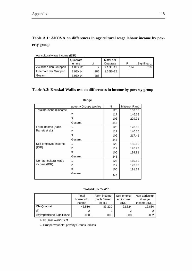
Appendix 118
Table A.1: ANOVA on differences in agricultural wage labour income by pov-
erty group
Agricultural wage income (IDR)
1.8E+12 2 9.13E+11 .674 .5103.9E+14 286 1.35E+123.9E+14 288
Zwischen den GruppenInnerhalb der GruppenGesamt
Quadratsumme df
Mittel derQuadrate F Signifikanz
Table A.2: Kruskal-Wallis test on differences in income by poverty group
Ränge
125 153.55117 146.68106 229.91348125 170.36117 140.05106 217.41348125 155.16117 176.77106 194.81348125 160.50117 173.80106 191.79
348
poverty Groups terciles123Gesamt123Gesamt123Gesamt123Gesamt
Total household income
Farm income (nachBarrett et al.)
Self-employed income(IDR)
Non-agricultural wageincome (IDR)
N Mittlerer Rang
Statistik für Testa,b
46.516 33.220 22.324 12.8302 2 2 2
.000 .000 .000 .002
Chi-QuadratdfAsymptotische Signifikanz
Totalhousehold
income
Farm income(nach Barrett
et al.)
Self-employed income
(IDR)
Non-agricultural wage
income (IDR)
Kruskal-Wallis-Testa.
Gruppenvariable: poverty Groups tercilesb.
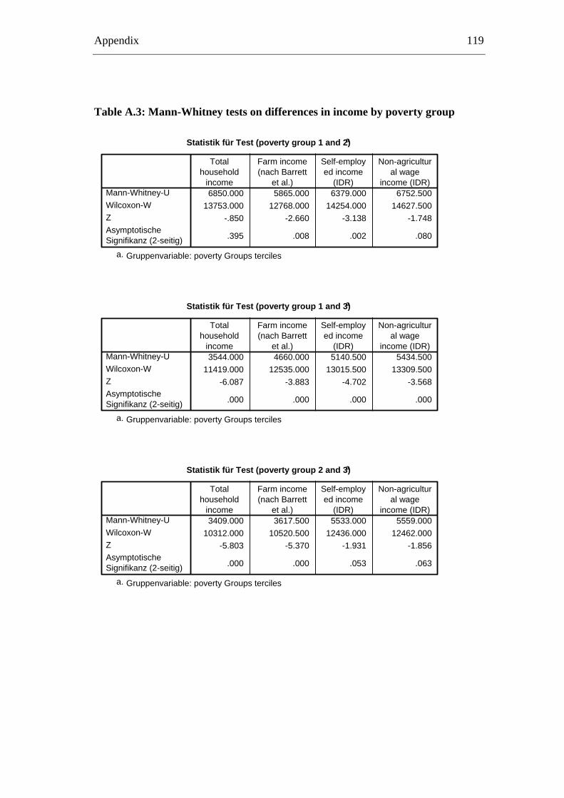
Appendix 119
Table A.3: Mann-Whitney tests on differences in income by poverty group
Statistik für Test (poverty group 1 and 2)a
6850.000 5865.000 6379.000 6752.50013753.000 12768.000 14254.000 14627.500
-.850 -2.660 -3.138 -1.748
.395 .008 .002 .080
Mann-Whitney-UWilcoxon-WZAsymptotischeSignifikanz (2-seitig)
Totalhousehold
income
Farm income(nach Barrett
et al.)
Self-employed income
(IDR)
Non-agricultural wage
income (IDR)
Gruppenvariable: poverty Groups tercilesa.
Statistik für Test (poverty group 1 and 3)a
3544.000 4660.000 5140.500 5434.50011419.000 12535.000 13015.500 13309.500
-6.087 -3.883 -4.702 -3.568
.000 .000 .000 .000
Mann-Whitney-UWilcoxon-WZAsymptotischeSignifikanz (2-seitig)
Totalhousehold
income
Farm income(nach Barrett
et al.)
Self-employed income
(IDR)
Non-agricultural wage
income (IDR)
Gruppenvariable: poverty Groups tercilesa.
Statistik für Test (poverty group 2 and 3)a
3409.000 3617.500 5533.000 5559.00010312.000 10520.500 12436.000 12462.000
-5.803 -5.370 -1.931 -1.856
.000 .000 .053 .063
Mann-Whitney-UWilcoxon-WZAsymptotischeSignifikanz (2-seitig)
Totalhousehold
income
Farm income(nach Barrett
et al.)
Self-employed income
(IDR)
Non-agricultural wage
income (IDR)
Gruppenvariable: poverty Groups tercilesa.
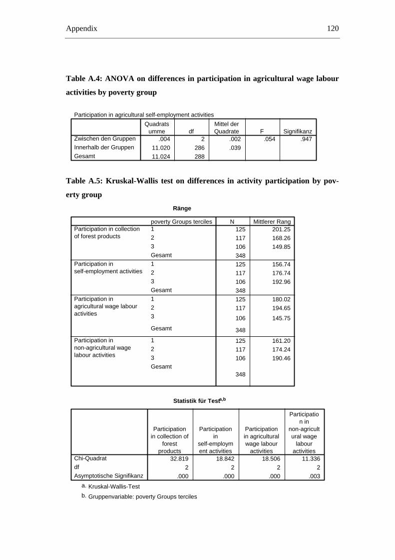
Appendix 120
Table A.4: ANOVA on differences in participation in agricultural wage labour
activities by poverty group
Participation in agricultural self-employment activities
.004 2 .002 .054 .94711.020 286 .03911.024 288
Zwischen den GruppenInnerhalb der GruppenGesamt
Quadratsumme df
Mittel derQuadrate F Signifikanz
Table A.5: Kruskal-Wallis test on differences in activity participation by pov-
erty group
Ränge
125 201.25117 168.26106 149.85348125 156.74117 176.74106 192.96348125 180.02117 194.65
106 145.75
348
125 161.20117 174.24106 190.46
348
poverty Groups terciles123Gesamt123Gesamt123
Gesamt
123Gesamt
Participation in collectionof forest products
Participation inself-employment activities
Participation inagricultural wage labouractivities
Participation innon-agricultural wagelabour activities
N Mittlerer Rang
Statistik für Testa,b
32.819 18.842 18.506 11.3362 2 2 2
.000 .000 .000 .003
Chi-QuadratdfAsymptotische Signifikanz
Participationin collection of
forestproducts
Participationin
self-employment activities
Participationin agriculturalwage labour
activities
Participation in
non-agricultural wage
labouractivities
Kruskal-Wallis-Testa.
Gruppenvariable: poverty Groups tercilesb.
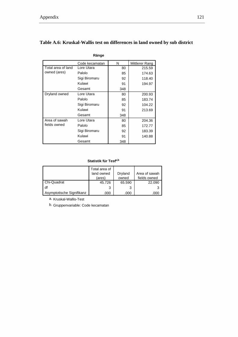
Appendix 121
Table A.6: Kruskal-Wallis test on differences in land owned by sub district
Ränge
80 215.5985 174.6392 118.4091 194.97
34880 200.9385 183.7492 104.2291 213.69
34880 204.3685 172.7792 183.3991 140.88
348
Code kecamatanLore UtaraPaloloSigi BiromaruKulawiGesamtLore UtaraPaloloSigi BiromaruKulawiGesamtLore UtaraPaloloSigi BiromaruKulawiGesamt
Total area of landowned (ares)
Dryland owned
Area of sawahfields owned
N Mittlerer Rang
Statistik für Testa,b
45.726 65.590 22.0903 3 3
.000 .000 .000
Chi-QuadratdfAsymptotische Signifikanz
Total area ofland owned
(ares)Drylandowned
Area of sawahfields owned
Kruskal-Wallis-Testa.
Gruppenvariable: Code kecamatanb.
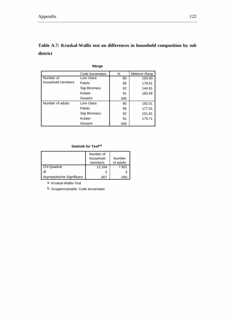
Appendix 122
Table A.7: Kruskal-Wallis test on differences in household composition by sub
district
Ränge
80 193.8385 178.6192 144.9191 183.58
34880 192.0185 177.0192 151.8191 179.71
348
Code kecamatanLore UtaraPaloloSigi BiromaruKulawiGesamtLore UtaraPaloloSigi BiromaruKulawiGesamt
Number ofhousehold members
Number of adults
N Mittlerer Rang
Statistik für Testa,b
12.164 7.8013 3
.007 .050
Chi-QuadratdfAsymptotische Signifikanz
Number ofhouseholdmembers
Numberof adults
Kruskal-Wallis-Testa.
Gruppenvariable: Code kecamatanb.
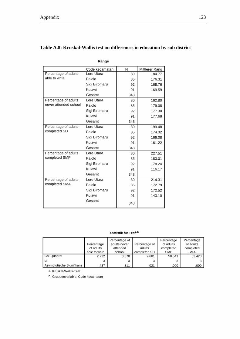
Appendix 123
Table A.8: Kruskal-Wallis test on differences in education by sub district
Ränge
80 184.7785 176.3192 168.7691 169.59
34880 162.8085 179.0892 177.3091 177.68
34880 199.4885 174.3292 166.0891 161.22
34880 227.5185 183.0192 178.2491 116.17
34880 214.3185 172.7992 172.5291 143.10
348
Code kecamatanLore UtaraPaloloSigi BiromaruKulawiGesamtLore UtaraPaloloSigi BiromaruKulawiGesamtLore UtaraPaloloSigi BiromaruKulawiGesamtLore UtaraPaloloSigi BiromaruKulawiGesamtLore UtaraPaloloSigi BiromaruKulawiGesamt
Percentage of adultsable to write
Percentage of adultsnever attended school
Percentage of adultscompleted SD
Percentage of adultscompleted SMP
Percentage of adultscompleted SMA
N Mittlerer Rang
Statistik für Testa,b
2.722 3.578 9.681 58.541 33.4233 3 3 3 3
.437 .311 .021 .000 .000
Chi-QuadratdfAsymptotische Signifikanz
Percentageof adults
able to write
Percentage ofadults never
attendedschool
Percentage ofadults
completed SD
Percentageof adults
completedSMP
Percentageof adults
completedSMA
Kruskal-Wallis-Testa.
Gruppenvariable: Code kecamatanb.
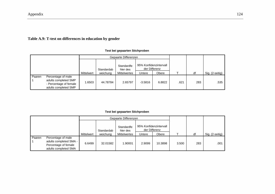
Appendix 124
Table A.9: T-test on differences in education by gender
Test bei gepaarten Stichproben
1.6503 44.78784 2.65797 -3.5816 6.8822 .621 283 .535
Percentage of maleadults completed SMP- Percentage of femaleadults completed SMP
Paaren1
MittelwertStandardabweichung
Standardfehler des
Mittelwertes Untere Obere
95% Konfidenzintervallder Differenz
Gepaarte Differenzen
T df Sig. (2-seitig)
Test bei gepaarten Stichproben
6.6499 32.01582 1.90001 2.9099 10.3898 3.500 283 .001
Percentage of maleadults completed SMA -Percentage of femaleadults completed SMA
Paaren1
MittelwertStandardabweichung
Standardfehler des
Mittelwertes Untere Obere
95% Konfidenzintervallder Differenz
Gepaarte Differenzen
T df Sig. (2-seitig)
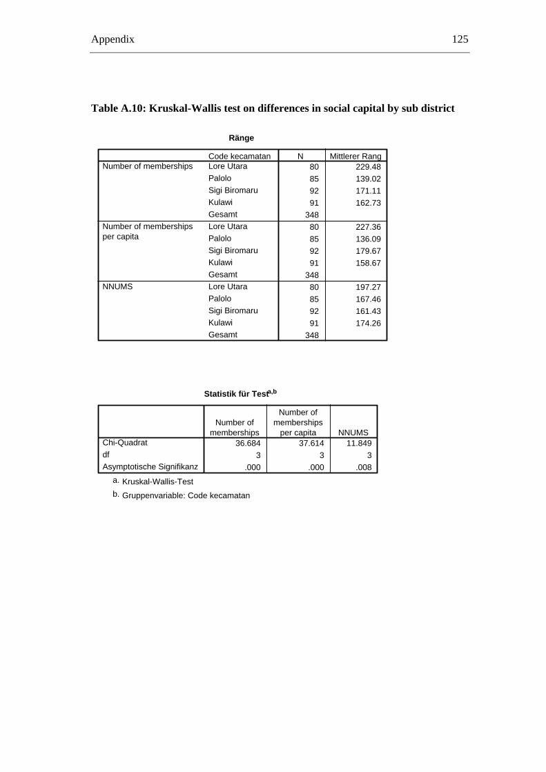
Appendix 125
Table A.10: Kruskal-Wallis test on differences in social capital by sub district
Ränge
80 229.4885 139.0292 171.1191 162.73
34880 227.3685 136.0992 179.6791 158.67
34880 197.2785 167.4692 161.4391 174.26
348
Code kecamatanLore UtaraPaloloSigi BiromaruKulawiGesamtLore UtaraPaloloSigi BiromaruKulawiGesamtLore UtaraPaloloSigi BiromaruKulawiGesamt
Number of memberships
Number of membershipsper capita
NNUMS
N Mittlerer Rang
Statistik für Testa,b
36.684 37.614 11.8493 3 3
.000 .000 .008
Chi-QuadratdfAsymptotische Signifikanz
Number ofmemberships
Number ofmemberships
per capita NNUMS
Kruskal-Wallis-Testa.
Gruppenvariable: Code kecamatanb.
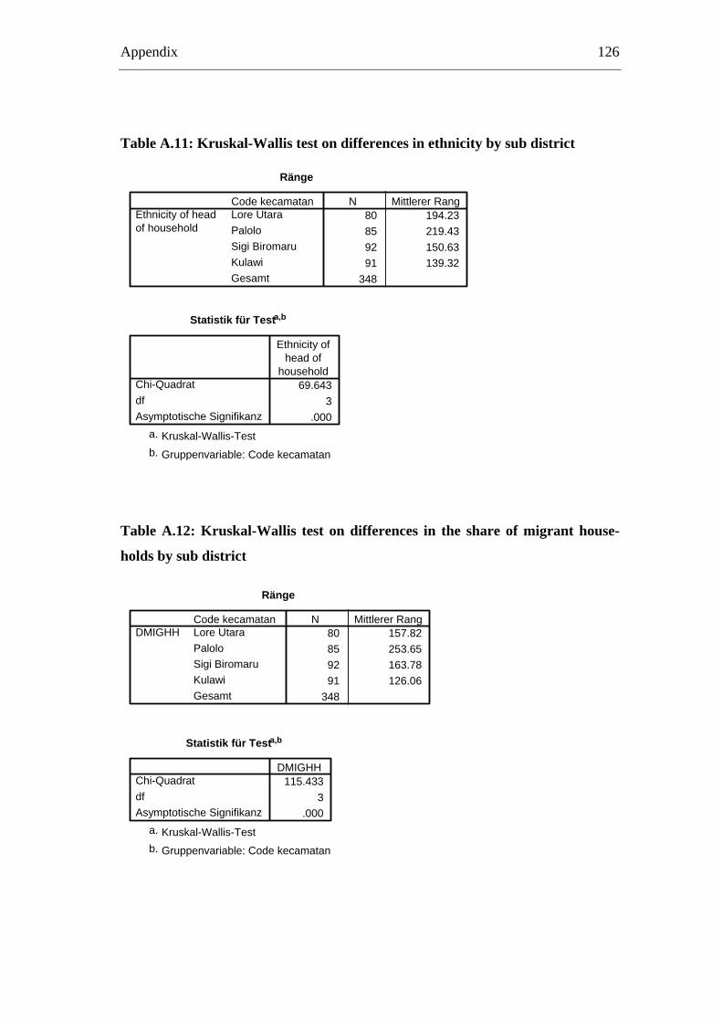
Appendix 126
Table A.11: Kruskal-Wallis test on differences in ethnicity by sub district
Ränge
80 194.2385 219.4392 150.6391 139.32
348
Code kecamatanLore UtaraPaloloSigi BiromaruKulawiGesamt
Ethnicity of headof household
N Mittlerer Rang
Statistik für Testa,b
69.6433
.000
Chi-QuadratdfAsymptotische Signifikanz
Ethnicity ofhead of
household
Kruskal-Wallis-Testa.
Gruppenvariable: Code kecamatanb.
Table A.12: Kruskal-Wallis test on differences in the share of migrant house-
holds by sub district
Ränge
80 157.8285 253.6592 163.7891 126.06
348
Code kecamatanLore UtaraPaloloSigi BiromaruKulawiGesamt
DMIGHHN Mittlerer Rang
Statistik für Testa,b
115.4333
.000
Chi-QuadratdfAsymptotische Signifikanz
DMIGHH
Kruskal-Wallis-Testa.
Gruppenvariable: Code kecamatanb.
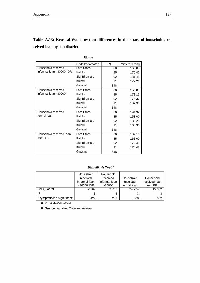
Appendix 127
Table A.13: Kruskal-Wallis test on differences in the share of households re-
ceived loan by sub district
Ränge
80 168.0585 175.4792 181.4891 172.21
34880 158.8885 178.1992 176.3791 182.90
34880 194.3285 153.0092 183.2691 168.30
34880 189.1085 163.0092 172.4691 174.47
348
Code kecamatanLore UtaraPaloloSigi BiromaruKulawiGesamtLore UtaraPaloloSigi BiromaruKulawiGesamtLore UtaraPaloloSigi BiromaruKulawiGesamtLore UtaraPaloloSigi BiromaruKulawiGesamt
Household receivedinformal loan <30000 IDR
Household receivedinformal loan >30000
Household receivedformal loan
Household received loanfrom BRI
N Mittlerer Rang
Statistik für Testa,b
2.769 3.757 24.724 15.3023 3 3 3
.429 .289 .000 .002
Chi-QuadratdfAsymptotische Signifikanz
Householdreceived
informal loan<30000 IDR
Householdreceived
informal loan>30000
Householdreceived
formal loan
Householdreceived loan
from BRI
Kruskal-Wallis-Testa.
Gruppenvariable: Code kecamatanb.