Master of Science Thesis in Electrical EngineeringDepartment of Electrical Engineering, Linköping University, 2020

Detection of Long TermVibration Deviations in GasTurbine Monitoring Data

Johan Hansson

Master of Science Thesis in Electrical Engineering

Detection of Long Term Vibration Deviations in Gas Turbine Monitoring Data:

Johan Hansson

LiTH-ISY-EX--20/5298--SE

Supervisor: Pavel Anistratovisy, Linköping University

Andreas HanssonSiemens Industrial Turbomachinery AB

Examiner: Erik Friskisy, Linköping University

Division of Vehicular SystemsDepartment of Electrical Engineering

Linköping UniversitySE-581 83 Linköping, Sweden

Copyright © 2020 Johan Hansson

Abstract

Condition based monitoring is today essential for any machine manufacturer tobe able to detect and predict faults in their machine fleet. This reduces the main-tenance cost and also reduces machine downtime. In this master’s thesis twoapproaches are evaluated to detect long term vibration deviations also called vi-bration anomalies in Siemens gas turbines of type SGT-800. The first is a simplerule-based approach where a series of CUSUM test are applied to several sig-nals in order to check if the an vibration anomaly has occurred. The secondapproach uses three common machine learning anomaly detection algorithm todetects these vibration anomalies. The machine learning algorithms evaluatedare k-means clustering , Isolation Forest and One-class SVM. This master’s thesisconclude that these vibration anomalies can be detected with these ML modelsbut also with the rule-based model with different levels of success. A set of fea-tures was also obtained that was the most important for detection of vibrationanomalies. This thesis also presents which of these models are the best suitedanomaly detection and would be the most appropriate for Siemens to implement.

iii

Acknowledgments

This master’s thesis has been written at Siemens Industrial Turbomachinery AB.I want to thank all of the colleagues at Siemens for interesting insights and helpthroughout this masters thesis. I also want to thank my supervisor at SiemensAndreas Hansson and the department manager Fredrik Tengvall for all the helpand pushing me in the right direction.

I also want to thank my examiner Erik Frisk for valuable insights. Last but notleast I want thank Pavel Anistratov my supervisor at Linköping University for alot of valuable discussions and proofreading of this masters thesis.

Norrköping, May 2020Johan Hansson

v

Contents

Notation ix

1 Introduction 11.1 Problem Formulation . . . . . . . . . . . . . . . . . . . . . . . . . . 21.2 Delimitations . . . . . . . . . . . . . . . . . . . . . . . . . . . . . . . 2

2 Background 32.1 Industrial Gas Turbines . . . . . . . . . . . . . . . . . . . . . . . . . 32.2 Vibration Measurements . . . . . . . . . . . . . . . . . . . . . . . . 52.3 Vibration Anomalies . . . . . . . . . . . . . . . . . . . . . . . . . . 72.4 Operational Data . . . . . . . . . . . . . . . . . . . . . . . . . . . . 82.5 Related Work . . . . . . . . . . . . . . . . . . . . . . . . . . . . . . . 10

3 Theory 113.1 CUSUM . . . . . . . . . . . . . . . . . . . . . . . . . . . . . . . . . . 113.2 K-means Clustering . . . . . . . . . . . . . . . . . . . . . . . . . . . 113.3 Support Vector Machine . . . . . . . . . . . . . . . . . . . . . . . . 13

3.3.1 One-class Support Vector Machine . . . . . . . . . . . . . . 153.4 Isolation Forest . . . . . . . . . . . . . . . . . . . . . . . . . . . . . 153.5 Dimensionality reduction . . . . . . . . . . . . . . . . . . . . . . . . 163.6 Normalization . . . . . . . . . . . . . . . . . . . . . . . . . . . . . . 183.7 Performance Evaluation . . . . . . . . . . . . . . . . . . . . . . . . . 18

4 Method 194.1 Tools and Frameworks . . . . . . . . . . . . . . . . . . . . . . . . . 194.2 Rule-Based Model . . . . . . . . . . . . . . . . . . . . . . . . . . . . 19

4.2.1 Parameters and Thresholds . . . . . . . . . . . . . . . . . . 204.3 ML models . . . . . . . . . . . . . . . . . . . . . . . . . . . . . . . . 20

4.3.1 Feature Selection . . . . . . . . . . . . . . . . . . . . . . . . 204.3.2 Pre-Processing . . . . . . . . . . . . . . . . . . . . . . . . . . 224.3.3 Parameters and Thresholds . . . . . . . . . . . . . . . . . . 23

4.4 K-means . . . . . . . . . . . . . . . . . . . . . . . . . . . . . . . . . 234.5 Isolation Forest . . . . . . . . . . . . . . . . . . . . . . . . . . . . . 25

vii

viii Contents

4.6 One-class SVM . . . . . . . . . . . . . . . . . . . . . . . . . . . . . . 254.7 Implementation . . . . . . . . . . . . . . . . . . . . . . . . . . . . . 264.8 Performance Evaluation . . . . . . . . . . . . . . . . . . . . . . . . . 264.9 Data Visualization . . . . . . . . . . . . . . . . . . . . . . . . . . . . 27

5 Results 295.1 Data Visualization . . . . . . . . . . . . . . . . . . . . . . . . . . . . 295.2 Rule-based Model . . . . . . . . . . . . . . . . . . . . . . . . . . . . 305.3 K-means Model . . . . . . . . . . . . . . . . . . . . . . . . . . . . . 315.4 Isolation Forest Model . . . . . . . . . . . . . . . . . . . . . . . . . 335.5 One-class SVM Model . . . . . . . . . . . . . . . . . . . . . . . . . . 355.6 Model Performances . . . . . . . . . . . . . . . . . . . . . . . . . . . 36

6 Discussion 416.1 Normalization . . . . . . . . . . . . . . . . . . . . . . . . . . . . . . 416.2 Models . . . . . . . . . . . . . . . . . . . . . . . . . . . . . . . . . . 416.3 Ground truth . . . . . . . . . . . . . . . . . . . . . . . . . . . . . . . 426.4 Related Work . . . . . . . . . . . . . . . . . . . . . . . . . . . . . . . 436.5 Future Work . . . . . . . . . . . . . . . . . . . . . . . . . . . . . . . 446.6 Results Usefulness . . . . . . . . . . . . . . . . . . . . . . . . . . . . 45

7 Conclusions 477.1 Thesis Questions . . . . . . . . . . . . . . . . . . . . . . . . . . . . . 47

Bibliography 49

Notation

Abbreviations

Abbrevation Meaning

rms Root Mean Squarerdc Remote Diagnostic Centrecusum Cumulative SUMsvm Support Vector Machineif Isolation Forestml Machine Learningpca Principal Component Analysissgt Siemens Gas Turbinetp True Positivesfp False Positivestn True Negativesfn False Negatives

ix

1Introduction

Siemens Industrial Turbomachinery AB today produces and serves a range of dif-ferent gas turbines. Today it’s crucial that faults are detected before they occur inthe gas turbine since otherwise a unplanned stops of the turbine will be needed.Siemens today monitors the turbines as a service to make the customers awareif the turbine shows an abnormal behavior. At the department Remote Diagnos-tic Center (RDC) the team performs daily monitoring of the turbines operationwhere everything ranging from lube oil pressure to the vibrations in the turbinesare supervised. Operational data for the different monitored turbines arrives ona daily basis and triggers a chain of analysis for detecting any abnormal behav-ior. The historical signals can then be viewed in an internal signal database. Allof this work at RDC is to provide a proactive diagnosis for the customers andavoiding unplanned stops of the customer turbine site.

One kind of abnormal behavior is long term vibration anomalies. These canbe seen as increasing vibrations over time or a change in trends. Not all increasesin vibrations are abnormal if they can be explained by the other signals such asan increase in load. Vibrations in turbines are normal and in it self not dangerousbut dangerous faults show up in vibrations. The goal for this master’s thesis is toevaluate different methods to detect deviations in long term vibration trends.

1

2 1 Introduction

1.1 Problem Formulation

The thesis aim is to answer the following questions:

• Can vibration anomalies be detected in available operational turbine dataat Siemens?

• Which methods are suitable for vibration anomaly detection?

• Which features are the most significant for vibration anomaly detection ingas turbines?

With the first question I wish to answer is the quality of the available turbine datagood enough to be able to detect vibration anomalies and can the developed mod-els detect these anomalies reliably. The second question aims to answer whichof these developed models are the best suited for this kind of anomaly detection.The third question aims to answer which of the available features or signals arethe most important for anomaly detection.

1.2 Delimitations

This master’s thesis is limited to detect vibration anomalies in the turbine of typeSGT-800. The turbines, which data has been gathered from are also situated inone region and run in similar conditions in terms of load profile and ambienttemperature to make the data as similar as possible. This is necessary to be ableto develop a fleet model for vibration anomaly detection.

2Background

2.1 Industrial Gas Turbines

Industrial gas turbines are used world wide. They can be used to either gener-ate electrical power to an energy grid or generate mechanical power to anothersystem such as a compressor. Siemens Industrial Turbomachinery AB producestoday a range of different industrial turbines but the turbine considered in thismaster’s thesis is the medium size gas turbine of class SGT-800, see Figure 2.1.This turbine class is sold world wide and its applications can vary from gas andoil industry to mining industry [23]. It’s a single shaft turbine engine and thedriveshaft extends from the core engine to the right into the gearbox to the left inFigure 2.1. The core engine is composed of three main components the compres-sor, combustor and turbine.

In Figure 2.1, the gearbox is to the far left. It connects to the driveshaft andto the generator which is not visible in the figure. The gearbox reduces the gasturbine shaft speed to a compatible shaft speed of the generator, the generatoroperates at around 1500 RPM for a 50 Hz electrical grid. The shaft speed of theturbine is around 6600 RPM. The next component to the right from the gearboxis the air duct where the gas turbine has its air inlet.

In Figure 2.2, a cross section view of the compressor, combustor and turbineis displayed. The compressor contain 15 stages of rotors and stators. One pair ofrotor and stator is considered as one stage. As the air passes through the differentstages the radius of the rotors and the slits in the stators gets smaller. The pres-sure of the air flowing through increases from 1 bar to 20 bar until the air finallyexits. The temperature of the air also increases as the air is compressed inside thecompressor. The compressor also has three variable guide vanes that can be usedto control the airflow. There are bleeding valves in case the compressor has torelease some of its compressed air. The purpose of the compressor is to increase

3

4 2 Background

Figure 2.1: Full view of a Siemens Industrial Gas Turbine of class SGT-800

the pressure of the air. An increase in air pressure together with an increase infiring temperature lead to an increase in thermal efficiency of the turbine to acertain degree [4]. There is a threshold where the efficiency will decrease with anincrease of air pressure for each gas turbine. Since the machine is a single axismachine as the compressor starts spinning the entire rotor starts spinning.

Compressed air then enters the combustor where a ring of burners ignites thegas with some of the compressed air to generate thrust. As the turbine combus-tor is ignited the turbine becomes idle and the ignition level increases until thethe sought level of operations is reached. When the sought level of operationis reached the generator switch is shut and the turbine is then operational. Thecombustor in a SGT-800 is annular which means that there is no separating wallbetween each burner. The idea behind this construction is to reduce the pressureloss and enable a smaller engine diameter [21]. The purpose of the combustor isto provide a highest possible firing temperature while at the same time keepingthe amount of nitrogen oxides (NOx) low in the exhaust gas. An increased firingtemperature in the combustor increases the amount of (NOx) [4]. The turbineconsist of three stages of rotor blades which has interlocking shrouds to reducevibrations. The rotor blades are thermally coated with special alloys to withstandthe temperatures created by the combustor. The turbine blades also have inter-nal cooling via channels trough the blade to further protect the blades from hightemperatures. The turbine is in turn connected to the driveshaft which enters thegearbox.

The generator then consist of a spinning magnet surrounded by coils. While

2.2 Vibration Measurements 5

Figure 2.2: Cross section view of a Siemens Industrial Gas Turbine of classSGT-800

the magnet is spinning the electrons in the coil are moving and thus creating acurrent. The magnet could have two poles or more. An increasing amount ofpoles in the magnet reduces the RPM needed of the spinning magnet. This isbecause the current would alternate faster with extra set of poles in the spinningmagnet. The generators connected to the SGT-800 turbines have in general twopoles.

2.2 Vibration Measurements

A vibration is an oscillatory movement around some reference point. Vibrationscan be measured as either a displacement (d), velocity (v) or as acceleration (a)and modeled with the following equations

d = A sin(wt + φ),

v = Aw cos(wt + φ),

a = −Aw2 sin(wt + φ).

(2.1)

Measurement metrics are defined differently depending what you are measuring.For acceleration, the metric is the peak shown in Figure 2.3 and for displacementit is the peak to peak. For velocity, the metric is obtained by calculating the root

6 2 Background

mean square (RMS) of the signal which is defined by

RMS =

√√√√√√(1/T )

T∫0

x(t)2. (2.2)

The different vibration measurements are used in different frequency ranges [4].For frequencies f ≤ 10 Hz, displacement is used while velocity is used for fre-quencies in the range 10 Hz≤ f ≤ 1000 Hz and acceleration for f ≥ 1000 Hz.A transducer transforms the mechanical vibration to a time-varying voltage out-

Figure 2.3: Timesignal showing the measurements Peak,Peak-Peak and RMS

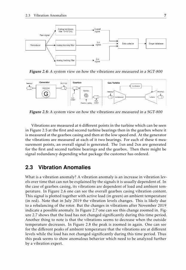
put [4]. The raw signal is then filtered by an analog filter to obtain the overallsignal which is the energy content of the raw signal with frequencies between 10-1000Hz. The 1xn and 2xn are the signals representing the energy content of theraw signal with frequencies one times the current rotor frequency and two timesthe current rotor frequency. They are obtained by applying a moving analog fil-ter which moves with the current rotor running-frequency also called a trackingfilter. The overall 1xn and 2xn signals are then stored in the data collector at theturbine site. The amplitude and phase of these signals are then sent to signaldatabase called STA-RMS where they can be monitored. This flow is shown inFigure 2.4.

2.3 Vibration Anomalies 7

Figure 2.4: A system view on how the vibrations are measured in a SGT-800

Figure 2.5: A system view on how the vibrations are measured in a SGT-800

Vibrations are measured at 6 different points in the turbine which can be seenin Figure 2.5 at the first and second turbine bearings then in the gearbox where itis measured at the gearbox casing and then at the low speed end. At the generatorthe vibrations are measured at each of it two bearings. For each of these 6 mea-surement points, an overall signal is generated. The 1xn and 2xn are generatedfor the first and second turbine bearings and the gearbox. Then there might besignal redundancy depending what package the customer has ordered.

2.3 Vibration Anomalies

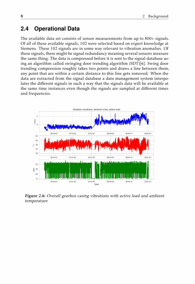
What is a vibration anomaly? A vibration anomaly is an increase in vibration lev-els over time that can not be explained by the signals it is usually dependent of. Inthe case of gearbox casing, its vibrations are dependent of load and ambient tem-perature. In Figure 2.6 one can see the overall gearbox casing vibration content.This signal is plotted together with active load (in green) an ambient temperature(in red). Note that in July 2019 the vibration levels changes. This is likely dueto a rebalancing of the rotor. But the changes in vibrations after November 2019indicate a possible anomaly. In Figure 2.7 one can see this change zoomed in. Fig-ure 2.7 shows that the load has not changed significantly during this time period.Another thing to note is that the vibrations seems to decrease when the outsidetemperature decreases. In Figure 2.8 the peak is zoomed in again. One can seefor the different peaks of ambient temperature that the vibrations are at differentlevels while the load has not changed significantly during this time period. Thusthis peak seems to show anomalous behavior which need to be analyzed furtherby a vibration expert.

8 2 Background

2.4 Operational Data

The available data set consists of sensor measurements from up to 800+ signals.Of all of these available signals, 102 were selected based on expert knowledge atSiemens. These 102 signals are in some way relevant to vibration anomalies. Ofthese signals, there might be signal redundancy meaning several sensors measurethe same thing. The data is compressed before it is sent to the signal database us-ing an algorithm called swinging door trending algorithm (SDT)[6]. Swing doortrending compression roughly takes two points and draws a line between them,any point that are within a certain distance to this line gets removed. When thedata are extracted from the signal database a data management system interpo-lates the different signals in such a way that the signals data will be available atthe same time instances even though the signals are sampled at different timesand frequencies.

Figure 2.6: Overall gearbox casing vibrations with active load and ambienttemperature

2.4 Operational Data 9

Figure 2.7: Zoom of overall gearbox casing vibrations with active load andambient temperature 2.6

Figure 2.8: A deeper zoom of overall gearbox casing vibrations with activeload and ambient temperature 2.7

10 2 Background

2.5 Related Work

The field of anomaly detection is an established field. The authors of [7] describeanomaly detection in the following way: "anomaly detection refers to the problemof finding patterns in data that do not conform to expected behavior". Anomalydetection is used in various fields such as machine fault detection, fraud detectionat credit card companies or network intrusion detection in network security. K-means clustering is used in [24] for network anomaly detection. The data set [24]consists of normal network data and network data when intrusions are made. In[24] k-means has the lowest accuracy but since the model is simple to implementit will still be considered in this master’s thesis. Isolation Forest has been appliedto detect gas path anomalies in gas turbines [26], where the authors has no labelsavailable and anomalies are few. This is the case for this master’s thesis as well. In[26] the Isolation Forest model performs well for gas path anomalies and needsno labels. Another approach is to create a model and predict the values of theavailable signals and then compare them to the observed values to determine ifthe data is anomalous or not [13]. The authors uses a Support Vector Regressionmodel that predicts performance signals in order to detect performance anoma-lies. A recurrent neural network has also been used for normal pattern extractionfor gas path analysis for gas turbines [2]. In [2] only normal data is available andthe authors develops an anomaly detection concept for this specific case. Goodaccuracy was achieved for both faulty data and normal data. One-class SVM hasalso been used for machine fault detection [22]. In [22], One-class SVM is ap-plied to rotating machinery which is a similar case to this master’s thesis. Theauthors in [22] concluded that One-class SVM is competitive in terms of anomalydetection with neural networks.

3Theory

This contains a brief summary of the theory behind the different methods usedthroughout the master’s thesis. Methods range from Machine Learning (ML) mod-els such as K-means and Isolation Forest (IF) to dimension reduction techniquessuch as Principal Component Analysis (PCA).

3.1 CUSUM

The Cumulative SUM (CUSUM) is a common algorithm for signal change detec-tion [17] . The algorithm work by creating a test quantity Tk as

Tk+1 = max(Tk + sk , 0), T0 = 0, sk = |r | − ν, (3.1)

where ν is the drift factor and rk is the residual. The residual should be set up insuch a way that r = 0 when there is no change and r , 0 if there is a change. Thisgives the test quantity the property that it continues to increase as long as thereis a change. The residual is often r = y − y where y is the predicted value and y isthe observed value.

3.2 K-means Clustering

K-means is a popular unsupervised clustering method [8]. It’s an iterative clus-tering method which starts with guessing the placement of the k cluster centers.It then assigns the data points to the closest centers and then replaces the clustercenters depending on the distance average of the data points belonging to it. Itrepeats this process until the cluster centers doesn’t move [8]. The algorithm isdescribed in [8] as

11

12 3 Theory

1. Given a cluster assignment C, the cluster variance Equation 3.3 is mini-mized with respect to m1, .., mk thus gives the means of the newly assignedclusters Equation 3.2.

2. With a set of meansm1, .., mk , Equation 3.3 is then minimized; each observa-tion is getting assigned to its closest cluster mean. That is given by Equation3.4.

3. Step 1 and 2 are repeated until the assigned clusters doesn’t change.

xS =∑i∈S||xi −m||2 (3.2)

minC,mk

K1

K∑k=1

Nk∑C(i)=k

||xk −mk ||2 (3.3)

C(i) = argmin1≤k≤K ||xk −mk ||2 (3.4)

In the ideal case, the features are distributed as in Figure 3.1 where a distinctclustering is visible. However this it not usually the case since often more thanthree features are used and visualization of the clusters is no longer possible.

Figure 3.1: Two randomly generated clusters

3.3 Support Vector Machine 13

3.3 Support Vector Machine

The Support Vector Machine (SVM) is a supervised classification algorithm thattries to construct a linear boundary condition that separates the different classesof data. It does this by calculating the boundary condition that maximizes themargin between the two classes which is the distance between the dotted lineand the line in Figure 3.2. If the data points aren’t linearly separable as in Figure3.2, the algorithm tries to project the data to a higher dimension space using akernel function φ(x) to more easily separate the data points [8].

Figure 3.2: A SVM example

The algorithm is defined in [8] as follows. Let (x1, y1), ..., (xn, yn) be the train-ing data where xi ∈ Rp. The data points can either be of class -1 or 1. Let’s definethe hyperplane as {x : f (x) = xT β + β0} where β is a unit vector ||β|| = 1 and β0 isa constant. β is a vector which is orthogonal to the hyperplane. The margin M isdefined as the distance between the hyperplane and the nearest point belongingto either class. It can be seen in Figure 3.2 as the distance between the either ofthe dotted lines to the hyperplane which is the line between them. The problemcan then be written as

maxβ,β0,||β||

M

subject to yi(xT β + β0) ≥ M, i = 1, .., N ,

(3.5)

14 3 Theory

where yi ∈ {−1, 1}. yi is defined in such a way that yi = 1 if x belongs to +1 andyi = −1 if x belongs to −1. Since the margin is defined as 1/ ||β|| the problem canbe rewritten as following

minβ,β0,||β||

subject to yi(xT β + β0) ≥ 1, i = 1, .., N .

(3.6)

One then introduces a the slack variables ξ = {ξ1, ..., ξN } two handle that thetwo classes −1 and 1 overlap. The slack variable ξ is the proportional amount ofwhich the prediction f (xi) = xTi β + β0 is on the wrong side of its margin. Thisslack variable can then be introduced to Equation 3.6 which gives

minβ,β0,||β||

subject to yi(xT β + β0) ≥ 1, i = 1, .., N ,

ξi ≥ 0∑

ξ ≤ constant.

(3.7)

The next step is to re-express Equation 3.7 as a quadratic programming problem

minβ,β0,

12||β||2 + C

N∑i=1

ξi

subject to ξi ≥ 0, yi(xT β + β0) ≥ 1 − ξi , i = 1, .., N ,

(3.8)

where C is a cost parameter which replaces the constant in Equation 3.7. In thecase that the classes are separable, C = ∞. The solution is obtained by usingLagrange multipliers. The Lagrange primal function is defined in Equation 3.9.

LP = minβ,β0,ξi

12||β||2 + C

N∑i=1

ξi −N∑i=1

αi(yi(xT β + β0) − (1 − ξi)) −

N∑i=1

µiξi (3.9)

Then equation 3.9 is derivated with regards to β, β0, ξi and set to zero thatgives the following equations. By substituting Equation 3.10 into Equation 3.9one the gets the Lagrange dual problem which is shown in Equation 3.11.

β =N∑i=1

αiyixi

0 =N∑i=1

αiyi

αi = C − µi∀iαi , µi , ξi ≥ 0∀i

(3.10)

LD =N∑i=1

αi −12

N∑i=1

N∑i′=1

αiαi′yiyi′xTi xi (3.11)

3.4 Isolation Forest 15

This Lagrange dual problem is then solved. If the classes aren’t linearly separablethen a kernel function can be used to project the data to another plane. Onepopular kernel is the radial basis function kernel defined as

KRBF = exp(−γ ||x − x′ ||2). (3.12)

3.3.1 One-class Support Vector Machine

One-class support vector machine (SVM) is an unsupervised anomaly detectionalgorithm [1] and is a special case of the SVM already described. One-class SVMtries to create a boundary condition for separating normal points from anomalies.This can be seen in Figure 3.3. The algorithm works in a similar fashion to theSVM but instead of trying to isolate three or more classes the One-class SVM triesto isolate normal data from anomalous data. The problem is defined in a similarfashion to the SVM as

minβ,ξ,β0

12||β||2 − β0 +

1νN

N∑i=1

ξi

subject to ξi ≥ 0, yi(βTφ(xi)) ≥ β0 − ξi , i = 1, .., N ,

(3.13)

where ξ, is a slack variable and ν is a regularization parameter that controls thetrade off between the constant β0 and the slack variables ξ. ν sets an upper limiton the fraction of anomalies and lower limit on the number of support vectors.

3.4 Isolation Forest

Isolation Forest (IF) is an other unsupervised anomaly detection algorithm [14].The method works by trying to classify anomalies rather than normal data points.It does this by trying to isolate all data points and creates a tree structure. Thealgorithm does this by randomly selecting a feature and randomly splitting thatfeature. It then creates several more tree structures using the same process. Theidea is that anomalies are few and exist outside the cluster of normal data pointsand are thereby easier to isolate.

Isolation forest creates a tree structure called an isolation tree [14]. The nodesT, of the isolation tree either has no or two children Tl,Tr. The values from theparent node are divided into the child nodes using a test on a randomly selectedattribute q and a randomly selected split value p. This splitting of the data con-tinues until either the isolation tree reaches a height limit or all data points areisolated. Next the path length h(x) is defined as the number of edges of the threeone has to walk from the current position until one reaches the top node, i.e theroot node. The anomalous points will since they are easier to isolate end up closerto the root node and thus have a short path length. Then the average search pathin a binary search tree as

c(n) = 2H(n − 1) − (2(n − 1)/n), (3.14)

16 3 Theory

Figure 3.3: A One-class SVM example

where H(i) is estimated by ln(i) + 0.5772156649. With this, one can then intro-duce a score function as

s(x, n) = 2−E(h(x))c(n) . (3.15)

The score function s(x, n) gives a measure of how anomalous a sample is. A sam-ple with a score function value close to 1 is definitely anomalous while a samplewith a score function much smaller than 0.5 can be regarded as normal. If all offthe instances has a score function close to 0.5 the dataset does not have any clearanomalies.

3.5 Dimensionality reduction

To reduce the amount of features and improve model efficiency a dimensionalityreduction technique is applied to the data set before it is sent to the models calledprincipal components analysis (PCA) [8]. PCA attempts to reduce the dimensionsof the dataset by creating a new dataset from linear combinations of the originalfeatures. In Figure 3.4 the process of creating principal components is shown.The data seen in Figure 3.4 can be projected alongside any of the two principalcomponents. In Figure 3.5 the data is projected along the first principal compo-nent. The goal of the principal component analysis is to maximize the explained

3.5 Dimensionality reduction 17

(a) Data (b) Data with principal compo-nents

Figure 3.4: PCA example.

variance of the projected points.

Figure 3.5: Data projected along the first principal component.

18 3 Theory

3.6 Normalization

Since the ML models use Euclidean distances and the features are of differentsizes, it is necessary to normalize the data [18]. There are different scaling meth-ods available an one of them is min max scaling which is defined as

x′

=x −min(x)

max(x) −min(x). (3.16)

There is also a z-score normalization which is defined as

x′

=x − xσ

. (3.17)

where x and σ are the mean and standard deviation of the signal [18].

3.7 Performance Evaluation

There exists several metrics for performance evaluation such as precision, recall,accuracy and F1 [19]. These metrics use the counts of true positives (TP), falsepositives (FP), true negatives (TN) and false negatives (FN). These metrics aredefined as

Precision =TP

TP + FP(3.18)

Recall =TP

TP + FN(3.19)

F1 =TP

TP + (FP + FN)/2(3.20)

Accuracy =TP + TN

TP + FP + TN + FN(3.21)

4Method

This section explains and further elaborates on how the model and dataset areused. Two approaches for long term anomaly detection has been developed. Oneis a Rule-based model where a series of CUSUM test is used to generate alarms.The other approach is a data driven approach where three different ML models K-means, IF and One-class SVM has been implemented and applied to the dataset.

4.1 Tools and Frameworks

All of the code for this master’s thesis has been written in Python 3.7 using thePyCharm IDE [20][5]. Several Python frameworks has been used through out thismaster’s thesis but matplotlib and scikit-learn are worth to mention [12][16]. Mat-plotlib is an open source visualization framework for Python. All of the graphsand plots in this master’s thesis has been generated by using matplotlib. Scikit-learn is an open source ML framework for Python and contains a lot of function-alities. The framework contains the different ML models but also the dimension-ality reduction method PCA and the two normalization methods.

4.2 Rule-Based Model

This model uses the same logic for detecting anomalous vibration behavior as onewould check manually.

• Have all of the vibration signals changed significantly?

• Has the load not changed significantly during the same time period?

• Has the ambient temperature not changed significantly during the sametime period?

19

20 4 Method

If the answer to all of these questions are yes then the time period is likely ananomaly. One can see in Figure 4.1 an overview of the Rule-based model. In all

Figure 4.1: A system overview of how the rule based model approach works

of the CUSUM test a rolling mean has been used as the normal value. The driftparameter is also set differently depending on which signal the test tries to detecta change for since they all are of different sizes. For this model 8 signals hasbeen used which can be seen in Figure 4.1. This is because any more signals arenot needed to raise an alarm that the timestamp indicates an vibration anomaly.Before sending the signals to the model the data is filtered on active load onlyusing data which has a load over 20 MW to ensure that the turbine is running.

4.2.1 Parameters and Thresholds

For each of the CUSUM tests, the drift parameters are tuned as a fraction of thenormal value. The thresholds for the alarm where set by hand while testing onthe bad turbine.

4.3 ML models

The ML approach can be seen in Figure 4.2. The data is sent to three ML anomalydetection algorithms covered in Chapter 3.

4.3.1 Feature Selection

Before sending the data into the ML models a feature selection is done by select-ing the features which have an absolute correlation above 0.5 to one of the overallvibration signals. This is achieved by creating a correlation matrix for the databelonging to all of the good turbines and then looking at the correlation for oneoverall vibration signal at a time. The correlation matrix has in each of its rowsthe correlation for a specific signal in the dataset to the other signals and canbe seen in Figure 4.3. Any duplicates are then removed from the list of featureswhich results in a list of unique important features.

The features that are then used are:

4.3 ML models 21

Figure 4.2: A system overview of how the ML models approach works

• Bearing 1, overall vibration signal (b_n1_vib1_fs)

• Bearing 1, 1xn signal (bearing1_1xn_vib1_fs)

• Bearing 2, overall vibration signal (b_n2_vib1_fs)

• Bearing 2, 1xn vibration signal (bearing2_1xn_vib1_fs)

• Generator bearing 1, overall vibration signal (gen_b_vib1_fs)

• Generator bearing 2, overall vibration signal (gen_b2_vib1_fs)

• Generator bearing 1, temperature (generator_bearing1_temp_fs)

• Generator bearing 2, temperature (generator_bearing2_temp_fs)

• Rotor speed signal (speed_transducer_fs)

• Gearbox, 1xn vibration signal (gearbox_1xn_vib1_fs)

• Gearbox, 2xn vibration signal (gearbox_2xn_vib1_fs)

• Gearbox, low speed overall vibration signal (gearbox_gen_vib_fs)

• Gearbox, high speed overall vibration signal (gearbox_vib1_fs)

• Lube oil temperature (lube_oil_temp1_fs)

• Gearbox, temperature (gearbox_temp1_fs)

• Bearing 1, 2xn vibration signal (bearing1_2xn_vib1_fs)

• Lube oil tank pressure (lube_oil_tank_pressure_fs)

22 4 Method

Figure 4.3: The correlation matrix for most relevant features

4.3.2 Pre-Processing

The second step is to pre-process the data. A rolling mean was applied on theselected features with a window of 24 hours. The window size was obtained byincreasing the window size step by step while looking at the performance of themodels. The rolling mean takes a window with a specific size and takes the meanof the signal on this window. This is to smooth out the signals. Also the scope islong term changes which means that fast changes in the signals are not importantand should be removed if possible. Then the data set was filtered by removingall of the points which did not have an active load above 20 MW to ensure thatthe turbine is running. The dataset was then normalized by applying a min-maxscaler and a zscore scaler (see Section 3.6). The normalization is necessary tointroduce the signals to a common scale since the distribution of the signals mightdiffer and then it is problematic to measure similarities and differences [24]. Twonormalization methods where used to be able to evaluate which of them wherethe best suited and if they had an impact on the performance of the models. Toreduce the time complexity of models the normalized signals are transformedby a PCA model to check if the data set can be represented using fewer features.

4.4 K-means 23

In Figure 4.4 one can see the explainability of the variance with the number offeatures used for both minmax normalized features and zscore. By looking atthese plots one can conclude that 10 PCA components will be a good choice forno matter which normalization method is used.

(a) PCA for minmax normalized features (b) PCA for zscore normalized features

Figure 4.4: The explain-ability of the variance with an increasing amount offeatures for minmax and zscore normalized features

These 10 PCA components was then sent into each of the models.

4.3.3 Parameters and Thresholds

Each of the different ML models contain either some thresholds (k-means clus-tering case) or some parameters which gives an indication on how many alarmscan be accepted for the training data. The training data contains no indicationof vibration anomalies and every alarm is thus a false alarm. The contaminationparameter for IF, the ν parameter for One-class SVM and the thresholds for the k-means clustering are set in such a manner that there would be 0.1% false alarmsfor the training data. These parameters and thresholds was tuned by lookingat the model performance for different levels of contamination. The amount ofalarms for the different models increases if the contamination is increased anddecreases if it the contamination parameter is decreased. The contamination pa-rameter could not be set to be zero for the training data since then ML modelswould not generate any alarms for the tests.

4.4 K-means

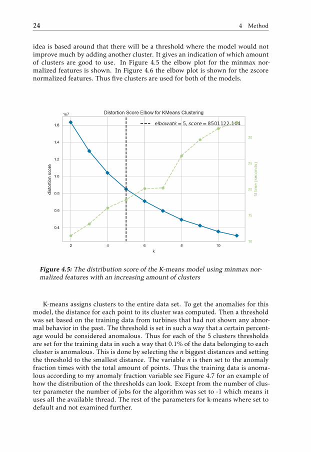
The K-means model that has been used is the one implemented by scikit learn[10]. Two models are created one where they both use features normalized byusing either minmax or zscore. First the number of desired clusters needed to becalculated. To get the optimal amount of clusters an elbow plot using was usedby applying the function provided from [25]. The elbow plot or elbow methodlooks at the explained variance as function of the number of clusters [3]. The

24 4 Method

idea is based around that there will be a threshold where the model would notimprove much by adding another cluster. It gives an indication of which amountof clusters are good to use. In Figure 4.5 the elbow plot for the minmax nor-malized features is shown. In Figure 4.6 the elbow plot is shown for the zscorenormalized features. Thus five clusters are used for both of the models.

Figure 4.5: The distribution score of the K-means model using minmax nor-malized features with an increasing amount of clusters

K-means assigns clusters to the entire data set. To get the anomalies for thismodel, the distance for each point to its cluster was computed. Then a thresholdwas set based on the training data from turbines that had not shown any abnor-mal behavior in the past. The threshold is set in such a way that a certain percent-age would be considered anomalous. Thus for each of the 5 clusters thresholdsare set for the training data in such a way that 0.1% of the data belonging to eachcluster is anomalous. This is done by selecting the n biggest distances and settingthe threshold to the smallest distance. The variable n is then set to the anomalyfraction times with the total amount of points. Thus the training data is anoma-lous according to my anomaly fraction variable see Figure 4.7 for an example ofhow the distribution of the thresholds can look. Except from the number of clus-ter parameter the number of jobs for the algorithm was set to -1 which means ituses all the available thread. The rest of the parameters for k-means where set todefault and not examined further.

4.5 Isolation Forest 25

Figure 4.6: The distribution score of the K-means model using zscore nor-malized features with an increasing amount of clusters

4.5 Isolation Forest

The IF model that is used is the one implemented by scikit learn [9]. Two mod-els are created using features from one of the two normalization methods. Thecontamination variable is used as a rough estimate on how many anomalies thetraining data has. Here it is set after some tuning to 0.1% which is the sameas the k-means model. I have also tested using different number of estimatorswhich is the number of Isolation trees in the model 100, 1000, 10000. The compu-tation time for the model increased as expected when increasing the number ofestimator and the accuracy does not seem to increase thus I kept 100 number ofestimators. The rest of the parameters where not examined any further but set totheir default value.

4.6 One-class SVM

The One-class SVM model that has been used is the one implemented by scikitlearn [11]. Two models are created using features from one of the two normal-ization methods. Since there are no labels it was quite an issue to tune the hyperparameters. The parameter ν is set in a similar fashion to the contaminationparameter in the IF model and uses the same anomaly fraction to 0.1%. The ker-nel that was used in the model was the radial basis function. The parameter γ

26 4 Method

Figure 4.7: The distribution of the distances to cluster 2 with the thresholdin red

which is the kernel coefficient was after some testing set to 10−6. The rest of theparameters where not examined and set to their default value.

4.7 Implementation

These models can be implemented in Siemens existing analysis tool and usedon daily monitoring data. This can be achieved by fetching the signals for theday which is to be analyzed and the day before. This is necessary since the rule-based model uses a rolling 1-day mean as the normal value for the signals andthe signals are pre-processed using a 1-day rolling mean in the ML models. Thusif no extra day is buffered the models will not have any data to analyze since therolling mean removes points which do not have a 1-day look back.

4.8 Performance Evaluation

To be able to evaluate the performance of the different models a ground truthis needed. For the faulty turbine the period where an vibration anomaly is in-

4.9 Data Visualization 27

dicated is considered as a true anomaly. This is visualized in Figure 4.8 wherethe anomalous data points are the points between the red lines indicating areas1 and 2. For the other two machines the assumption is that they do not have any

Figure 4.8: The overall gearbox vibration signal with the red lines as anindication where the anomalies are. The lower figure represent the actualground truth signal which is either zero or one.

vibration anomalies. This means that the precision, recall and F1 metrics are notavailable for these tests. This is because the TP and FP are both zero when theground truth has no alarms in it.

4.9 Data Visualization

To be able to visualize the different effects of the normalization methods and theeffect of the rolling mean, t-sne was applied to project the data to a 2-D plane[15]. The data was then labeled into different classes if it was normal data whichis the data used for training or normal data from either the good turbines or thebad turbine. Again here my guess of the ground truth is used (see Section 4.8)to determine if it is abnormal or not. Normal data is then compared with thenormal and abnormal data and to the normal data from the good turbines.

5Results

In this section contains the results from the two different approaches. The testshave been performed on one bad turbine, that indicates an vibration anomaly,two turbines without any indications of anomalies. These three turbines are newto the model and have not been available during training. The ML models havebeen trained on 3 months data from 12 different gas turbines that have no indica-tions of vibration anomaly.

5.1 Data Visualization

In Figure 5.1 the t-sne projections for the unfiltered dataset are shown. In Figure5.1 one can observe that the abnormal data points seem to be very close to thenormal data points from the bad turbine. The normal data from the bad turbineis also clearly distinguishable from the normal data from the training set. Thenormal data from the two normal machines seems to form two distinct clusters.In Figure 5.2 the dataset is visualized after using the rolling 24-h mean. Here onecan note that the rolling mean seems to smooth out the abnormal data points andseparate it from the normal data points from the bad turbine. It seems howeveras the abnormal data is closer to the normal training data. The normal data fromthe bad turbine seems to form clusters of it’s own but is also spread out more.The normal data from the two good turbine also gets spread out more comparedto Figure 5.1. In Figure 5.3 one can see the visualization of the minmax normal-ized features. One can note that the abnormal data points seems to form its ownclusters while its still close to the normal data from the bad turbine and normaldata from the training set. The different normal data seem to form separableclusters. The cluster belonging to good turbine 2 seems to be further away fromthe normal training data compared to the other good turbine. In Figure 5.4 thezscore normalized dataset is shown. Here one can note that the abnormal points

29

30 5 Results

form a distinct cluster outside the two other normal clusters. The normal datapoints also form its own separate clusters. The cluster of the normal data belong-ing to the good turbine 2 seem to be closer to the normal data from the trainingset compared to the normal data from good turbine 1.

(a) 2D visualization of normaltraining data with abnormal andnormal data from the bad turbine.

(b) 2D visualization of the normaltraining data with normal datafrom the two good turbines.

Figure 5.1: 2D t-sne projection of the unfiltered dataset.

(a) 2D visualization of normaltraining data with abnormal andnormal data from the bad turbine.

(b) 2D visualization of normaltraining data with the normaldata from the two good turbines.

Figure 5.2: 2D t-sne projection of the filtered dataset.

5.2 Rule-based Model

Figure 5.5 shows the test for the bad turbine where there are anomalies. In thisfigure the amounts of alarms is shown together with the accuracy of the modeland the F1 measure. One can see from the figure that the model generates acouple of false alarm in the region where the signal is low and when the signallevels changes. This observable change in signal mean is as already mentioned(Section 2.3) likely due to a re-balance of the rotor but this model detects a changehere since all of the vibration levels change after the re-balance. Since this data

5.3 K-means Model 31

(a) 2D visualization of normaltraining data with abnormal andnormal data from the bad turbine.

(b) 2D visualization of normaltraining data with the normaldata from the two good turbines.

Figure 5.3: 2D t-sne projection of the minmax normalized and filtereddataset.

(a) [2D visualization of normaltraining data with abnormal andnormal data from the bad turbine.

(b) 2D visualization of normaltraining data with the normaldata from the two good turbines.

Figure 5.4: 2D t-sne projection of the zscore normalized and filtered dataset.

is not filtered with a rolling mean, the signal varies more. But the actuary is stillquite good while the F1 score is quite low.

In Figure 5.6 the rule based model is tested on good turbine 1 that has noanomalies. Here one can note that the amounts of alarms is lower compared tothe previous test and the accuracy is higher since no alarms are expected for thistest.

In Figure 5.7 one can see the results on good turbine 2. The alarms for thismachine is even lower than the previous ones and thus the accuracy is highersince no alarm is expected for this signal as well.

5.3 K-means Model

In Figures 5.8, 5.9 and 5.10 the results for the k-means model are shown. In thesefigures one can see the amount of alarms generated together with the accuracy

32 5 Results

Figure 5.5: The Rule-based model applied to the bad turbine data.

Figure 5.6: The Rule-based model applied to the good turbine 1 data.

and F1 measures. In Figure 5.8 one can observe that the minmax normalizeddata alarms more frequently compared to the zscore normalized data. In this testtimestamps where an alarm should be raised according to my created groundtruth (see Figure 4.8) are after 2019-11 in Figure 5.8. The amount of false alarms

5.4 Isolation Forest Model 33

Figure 5.7: The Rule-based model applied to the good turbine 2 data.

is higher for the minmax normalized features compared to the zscore features.The accuracy measure measure are also better the zscore normalized featureswhile the F1 measure is slightly lower.

In Figure 5.9 one can see that the zscore normalized features generates analarm less frequently compared to the minmax normalized features. In this testno alarms are expected as mentioned in the Section 4.8. The accuracy is thuslower for the minmax normalized features. Since there are no expected alarmsthe precision and recall measures are not available.

In Figure 5.10 the results from the test from good turbine 2 is shown. Onecan note that the k-means model with zscore normalized features generates lessalarms compared to the other model. Since the expected result for this turbine isno alarm the accuracy for the k-means model with zscore normalized features isthe highest.

5.4 Isolation Forest Model

In Figures 5.11, 5.12 and 5.13 the results for the IF model are shown. In theseFigures the amounts of generated alarms are shown together with the accuracyand F1 measure. In Figure 5.11 one can see the results for the test on the badturbine for both minmax normalized features and zscore normalized features.

34 5 Results

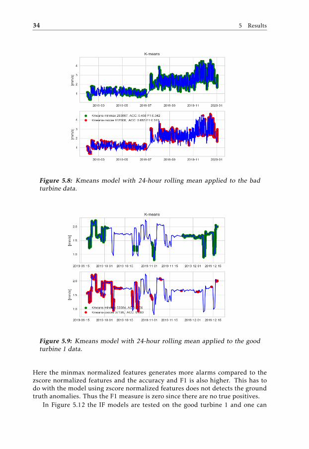
Figure 5.8: Kmeans model with 24-hour rolling mean applied to the badturbine data.

Figure 5.9: Kmeans model with 24-hour rolling mean applied to the goodturbine 1 data.

Here the minmax normalized features generates more alarms compared to thezscore normalized features and the accuracy and F1 is also higher. This has todo with the model using zscore normalized features does not detects the groundtruth anomalies. Thus the F1 measure is zero since there are no true positives.

In Figure 5.12 the IF models are tested on the good turbine 1 and one can

5.5 One-class SVM Model 35

Figure 5.10: Kmeans model with 24-hour rolling mean applied to the goodturbine 2 data.

note that the IF model with zscore nomralized features generates more alarmscompared to the model with minmax normalized features. The accuracy of themodel with zscore normalized features is lower then the models with minmaxnormalized features. Both of the models detect the alarms at the drop of thevibration signal.

In Figure 5.13 the two models are tested on the good turbine 2. One can notethat the model with zcore normalized features generates more alarms comparedto the model with minmax features. This is why the accuracy is better for themodel with minmax normalized features.

5.5 One-class SVM Model

The results for the different test for the one-class SVM model can be seen in Fig-ures 5.14, 5.15 and 5.16. In these figures the amounts of generated alarms areshown together with the accuracy and F1 measures. In Figure 5.14 the test onthe bad turbine is shown. One can note that the model using zscore normalizedfeatures generates more alarms and has higher accuracy and F1 measures.

In Figure 5.15 the test on good turbine 1 is shown. One can note that the bothof the models generate the same amount of alarms and has the same accuracy andF1 measures. The amounts of alarms generated are low thus the high accuracysince no alarms are expected.

In Figure 5.15 the test on good turbine 2 is shown. One can note that the bothof the models generate the same amount of alarms and has the same accuracy andF1 measures. The alarms generated in this test are also low just as the previoustest. Thus the high accuracy of the models are achieved.

36 5 Results

Figure 5.11: IF model with 24-hour rolling mean applied to the bad turbinedata.

Figure 5.12: IF model with 24-hour rolling mean applied to the good turbine1 data.

5.6 Model Performances

Tables 5.1 and 5.2 present the performance metrics for different tests. The k-means model has the highest recall even though the model has the worst accu-racy of all of the models. The precision for the k-means model is the lowest

5.6 Model Performances 37

Figure 5.13: IF model with 24-hour rolling mean applied to the good turbine2 data.

Figure 5.14: One-class SVM model with 24-hour rolling mean applied to thebad turbine data.

compared to the other ML models. The accuracy for the k-means model is theworst when it comes to the test on the two good machines. The One-class SVMmodel has good accuracy for the test on the bad turbine. Depending on whichnormalization approach the model uses, the model achieves really good resultsand quite bad results when comparing to the other models. The best results from

38 5 Results

Figure 5.15: One-class SVM model with 24-hour rolling mean applied to thegood turbine 1 data.

Figure 5.16: One-class SVM model with 24-hour rolling mean applied to thegood turbine 2 data.

the One-class SVM has the second best precision and accuracy for the test on thebad turbine. The model achieves the best accuracy for the good turbine 1. TheIF model also has different results depending on which normalization method isused. The best results has the highest precision, accuracy, F1 and recall measures.The performance on the two good turbines is good, it has accuracy slightly lower

5.6 Model Performances 39

Table 5.1: The test results for the bad turbine.

Test Precision Recall F1 AccuracyOneClassSVM_bad_minmax 0.2302 0.0796 0.1183 0.7879OneClassSVM_bad_zscore 0.7289 0.3441 0.4675 0.8599kmeans_bad_minmax 0.2184 0.7895 0.3421 0.4576kmeans_bad_zscore 0.2575 0.4106 0.3165 0.6831RuleBased_bad 0.1726 0.0195 0.0351 0.8272if_bad_minmax 0.9403 0.5160 0.6663 0.9076if_bad_zscore 0.0 0.0 0.0 0.8129

Table 5.2: The test results for the good turbine 1 and 2.

Test AccuracyOneClassSVM_good1_minmax 0.9961OneClassSVM_good1_zscore 0.9961OneClassSVM_good2_minmax 0.8678OneClassSVM_good2_zscore 0.8678kmeans_good1_minmax 0.5595kmeans_good1_zscore 0.6930kmeans_good2_minmax 0.1959kmeans_good2_zscore 0.8444if_good1_minmax 0.9835if_good1_zscore 0.9774if_good2_minmax 0.9869if_good2_zscore 0.9239RuleBased_good1 0.9758RuleBased_good2 0.9891

than One-class SVM when looking at the best results for IF. The rule-based modelhas a lower precision, recall and F1 compared to the ML models but has good ac-curacy for the test on the bad turbine. The accuracy for the tests on the two goodturbines are comparable to the One-class but slightly lower. When comparingthe accuracy for the rule-based model with the accuracy for the k-means modelthe rule-based model outperforms.

6Discussion

In this chapter the results and findings of this master’s thesis are presented anddiscussed.

6.1 Normalization

From the results in the previous chapter one can clearly see that the normaliza-tion method has an impact on the model performance. The zscore normalizationseems to be the best choice for the k-means models while the minmax normaliza-tion outperforms zscore for the IF model. When it comes to the One-class SVMthe zscore normalization achieves the best performance for both the bad turbineand the two good turbines.

6.2 Models

The results presented in Chapter 5 point that, by all the ML models, k-means hasthe worst performance. Since it generates alarms very frequently it has a good re-call score since it detects a lot of the anomalies but it also has the worst accuracywhen comparing with the other models (see Tables 5.1 and 5.2). The One-classSVM had the by far the longest training time and prediction time when using alow γ compared to the other two models. The One-class model performs bettercompared to the k-means when using zscore normalization. It has a high perfor-mance in the test on the bad machine while at the same time has the best accuracyfor the test on the good turbine 1. The rule-based model has good accuracy forthe bad turbine while at the same time having good accuracy for both of the goodturbines. What it lacks, however, is good precision since it doesn’t detect all ofanomalies. The IF model using minmax normalized features has the best perfor-

41

42 6 Discussion

mance of all of the models. It has high precision and good accuracy for the badturbine while at the same time it has good accuracy for both of the good turbine.

One reason why the k-means model does not perform as well as the other MLmodels can be that datapoints is not as close of the cluster centers as expected.The idea is that the normal data points should be close together near the clustercenter while the anomalies should be on the outside of the cluster center. Thecluster centers are calculated using the training data. Thus if the test data is not assimilar to the training data they will end up further out from the cluster centers.The k-means model generates alarms more frequently compared to the other MLmodels and quite frequently overall. This points to the thresholds set from thetraining data are to narrow and needs further development. From Figures 5.3and 5.4 one can see that the normal data from the two good turbines form theirown clusters instead of the data overlapping with the normal training data. Thiscould indicate that the normal data is not as similar as one would like them tobe. The different turbines used has a quite signals but the preconception wasthat they would be similar enough to form clusters of normal data which do notseem to happen since the k-means model alarms to frequently. The abnormaldata shown in Figures 5.3 and 5.4 does not seem to be that far away also from thetwo normal clusters in both of the figure. This can make it hard for the k-meansmodel to detect the abnormal data.

One has to have in mind that the IF model is by default random and thusone can not expect the same results from the same test. This is because the IFmodel splits the features randomly when trained to isolate each data points. Thusthe results from the IF model can be unreliable which has been observed in thismaster’s thesis. The results from the IF model shown in Section 5.4 is the bestresults achieved. Tests on the bad turbine where both of the models using eitherof the normalization method misses the anomalies has been observed.

One reason why the One-class SVM performs better using when using thezscore normalization method compared to the minmax features could be the howdistinct the abnormal data is. One can observe in Figures 5.3 and 5.4 that theabnormal data cluster seems to be more distinguishable from the normal datawhen using the zscore normalization compared to minmax normalization.

6.3 Ground truth

In Figure 4.8 the ground truth for the bad turbine is shown. In this master’s thesisall of the points in region 1 and 2 are considered true anomalies but are they partof one anomalous occurrence or are there two separate occurrences one in each re-gion. It seems as there are to separate occurrences since the vibration levels dropsback to normal in between. By comparing the results from the models to Figure4.8 all of the models detect both of these occurrences but with different amountsof false alarms in between. The rule-based method alarms both on the vibrationincreases but also the vibration decrease. The k-means model generates alarmsthroughout both of the occurrences but since it generates an alarm frequentlyit also generates false alarms between and after the occurrences. The IF model

6.4 Related Work 43

detects both of the occurrences and also generates some false alarms but not asmany as the k-means model. The One-class SVM detects both of the occurrenceswhile at the same time few false alarms if any around the two occurrences.

6.4 Related Work

The approach proposed in this master’s thesis differs a bit from some of the workmentioned in Section 2.5. The approach in [26] uses a series of IF models withdifferent levels of contamination to group the dataset into groups of normal dataand abnormal data. This has not been attempted in this master’s thesis. Insteada simpler approach is used which considers each point of the dataset in termsof if it is abnormal or normal. As mentioned in Section 6.2 the IF model canbe miss vibration anomalies but can achieve high performance when vibrationanomalies are detected. The authors of [26] find that it is a good option for gasturbine gas path anomalies. The authors of [26] achieves precision, recall and F1performance of around 94% compared to this thesis which best results has 94%precision and recall of 51% and recall 66% F1. Thus the model from [26] clearlyperforms better. One reason for this can be that the gas path anomalies are moreanomalous than vibration anomalies and are thus easier to detect.

In [13] the authors also use a filtering method to do the feature selection, butsince the scope of that article is flight performance, the flight dynamic featureswhere used. In this master’s thesis since the scope is vibration anomalies theoverall vibration signals was used instead. The Support Vector Regression modelused in [13] predicts the flight dynamics feature values and evaluates the pre-dicted value with the observed value to check whether the point is anomalous ornot. The scope of [13] also concerns fast dynamic changes which differs from thismaster’s thesis which looks at long term changes. In [2] the approach is insteadto find features that will remain unchanged during normal conditions and pre-dict that feature using a recurrent neural network to detect gas path anomalies.Since both [2] and [13] predicts signals the performance metrics are in terms ofhow well the signal was predicted. Thus the the results of [2] and [13] can not bedirectly compared to this master’s thesis results.

In [24] the authors uses a k-means model to detect network intrusions. Thedataset used in [24] uses a dataset with duplicated records. This was never at-tempted in this master’s thesis since it was realized at a late stage of the thesisthat this could be useful. One could duplicate the data from the bad machineand add a Gaussian noise to get new faulty data. The authors of [24] achieves anaccuracy of around 58% and a false alarm ratio of approximate 23%. This canbe compared to the k-means results for the bad turbine with an accuracy of 68%and a false alarm rate around 15 − 30%. Thus an higher accuracy is achieved inthis masters thesis but a bigger false alarm rate is observed for the good turbine 1.

In [22] the authors use One-class SVM to detect faults in rotating machinery.

44 6 Discussion

The difference between the approach is that the authors of [22] has a supervisedproblem for a single machine while this master’s thesis propose an unsupervisedapproach for a fleet of machines. The results from [22] point out that One-classSVM is a good model to use for machine fault detection while this thesis resultspoint out that to One-class SVM is decent at detecting vibration anomalies. Theauthors of [22] use different performance metrics compared to this master’s the-sis but one can still conclude that they achieve better results. This could due toOne-class SVM performing better with supervised problems compared to unsu-pervised.

6.5 Future Work

Since the vibration levels for the different turbines are quite unique and not assimilar as one would hope anomaly detection using unsupervised learning al-gorithms is difficult. An idea to improve it is to make some kind of regressionmodel or models to predict the different vibrations levels. One can then createa residual with the observed value and subtract the predicted value. One canthen set an alarm when the difference exceeds a threshold. The benefit of doingthis is that the vibrations signals is available at Siemens signal database thus thetrue value of the vibrations is known. This approach is attempted in [13][2] withsome differences. The idea to predict a features which would remain the samein normal conditions seems like good idea to investigate for vibration anomalydetection. Here the overall signals can probably be used since they contain theentire vibration content.

Since the amount of indicated anomalies in the data are few another idea onhow to improve the data set is to inject a vibration anomaly. This can be done byincreasing the overall vibration signals with a step for a certain amount of time.Thus more test with an anomaly will be available and increase the reliability ofthe performance measures. One could also duplicate the bad turbine data whichis done in [24] and then apply a Gaussian noise to it. Then new faulty data wouldbe available to work with.

It would be great if the employees working with the daily monitoring couldmark a part of the turbine data that is anomalous. This would enable a supervisedmodel approach to be used but this will lead to another question how should itbe labeled. Here it will be good if all of the different faults and or anomalousbehaviors had its own label. It seems wise to separate the anomalies in groupssuch as sensor anomalies and vibration anomalies. A good idea would be to startwith the anomalies that are the most troublesome finding manually.

One more idea that could be looked into is to make machine specific modelsfor vibration anomaly detection. One feature that is available but has not beenused is the phase signal for the 1xn and 2xn. The vibration experts at Siemenslook at both the vibration magnitude and the angle or phase of the vibration andrepresent vibrations as vectors in a 2-d space. This vibration signature is uniquefor each of the turbine thus it has not been used through out this master’s thesisbut will be really good to use for modeling normal behavior of a single machine.

6.6 Results Usefulness 45

What has not been explored in this master’s thesis and could improve the mod-els are handcrafting features. One could be done is to create new features fromthe available ones to obtain features that can be used for better vibration anomalydetection. This however requires domain knowledge with turbine vibrations andcould possibly be done with help from the vibration experts at Siemens.

6.6 Results Usefulness

The results provided in Chapter 5 show that to a certain extent vibration anoma-lies can be detected using the models proposed in this master’s thesis. Betterperformance can be achieved by implemented some of the proposed methods inthe previous section. The next step would be to develop new models for detectingnew kinds of anomalies in other signals. Gas path anomalies seems to be good tostart with since some research has already been done in this field. One could alsodesigning models for specific turbine faults. One problem with this is that faultymachine data are rare but could be overcome by injecting this faults in the turbinedata. The need for good diagnostics models, data driven such as the ML modelsor rule-based are crucial for conditioned based maintenance. Conditioned basedmaintenance would allow for a reduction in maintenance cost and increase ofturbine uptime which is critical for good profitability for both Siemens and itscustomers.

7Conclusions

This chapter will give the reached conclusions regarding the thesis questions seeSection 1.1 and the master’s thesis as a whole.

7.1 Thesis Questions

Can vibration anomalies be detected in available operational turbine data atSiemens? Yes, vibration anomalies can be detected but with different levels ofreliability depending on which of the models are used. One also has to have inmind that the results from the different models stems from a guess when creatingthe ground truth (see Section 4.8). Thus the performance of the models onlybecomes as accurate as the guess of where the anomalies are.

Which methods are suitable for vibration anomaly detection? When com-paring the different ML models one can clearly see that the IF model seems tohave the best performance and has a low execution time compared to k-meansand One-class SVM models. However it is slightly undependable since the re-sults from the model cannot be expected to be the same from test run to test run.This is because in the training the model randomly splits of the features to de-tect anomalies. The One-class SVM has the second best performance but has ahigh training and predicting time compared to the other ML models. Howeverthe performance of the rule-based method is also good when looking at the twogood turbines. When taking in mind how this model will be implemented andused in practice the rule-based approach has an advantage of being simple to im-plement and being simple to explain for the end users at RDC. The ML modelswill inevitably be harder to implement and harder to explain for the end userwho lacks machine learning domain knowledge. The ML model is also likely torequire more maintenance since it is more complex. Thus when taking this intoconsideration the rule-based model seems to be the best choice.

47

48 7 Conclusions

Which features are the most significant for vibration anomaly detection ingas turbines? The overall vibration signals shows the vibration entire vibrationcontent for different parts of the turbine. Since this masters thesis is limited todetect anomalies in the vibrations its seems reasonable to use the signals whichhas the highest absolute correlation to the overall vibration signals. If this was asupervised problem one could then use different sets of signals or features andcheck the model output and keep the ones with the pest performance. But sinceno true amount of anomalies are available and this being an unsupervised ap-proach this is not possible. The list of features which where found to be the mostimportant are found can be seen in Section 4.3.1.

Bibliography

[1] Mennatallah Amer, Markus Goldstein, and Slim Abdennadher. Enhancingone-class support vector machines for unsupervised anomaly detection. InProceedings of the ACM SIGKDD Workshop on Outlier Detection and De-scription, ODD ’13, pages 8–15, New York, NY, USA, 2013. ACM.

[2] Mingliang Bai, Jinfu Liu, Jinhua Chai, Xinyu Zhao, and Daren Yu. Anomalydetection of gas turbines based on normal pattern extraction. Applied Ther-mal Engineering, 166:114664, 2020.

[3] Purnima Bholowalia and Arvind Kumar. Ebk-means: A clustering techniquebased on elbow method and k-means in wsn. International Journal of Com-puter Applications, 105(9), 2014.

[4] Meherwan P Boyce. Gas turbine engineering handbook. Elsevier, 2011.

[5] JET BRAINS. Pycharm ide. https://www.jetbrains.com/pycharm/,Mars 2020. Accessed on 2020-03-28.

[6] Edgar H Bristol. Data compression for display and storage, May 26 1987.US Patent 4,669,097.

[7] Varun Chandola, Arindam Banerjee, and Vipin Kumar. Anomaly detection:A survey. ACM computing surveys (CSUR), 41(3):1–58, 2009.

[8] T. Hastie, R. Tibshirani, and J.H. Friedman. The Elements of StatisticalLearning: Data Mining, Inference, and Prediction. Springer series in statis-tics. Springer, 2009.

[9] Scikit learn. Isolation forest. https://scikit-learn.org/stable/modules/generated/sklearn.ensemble.IsolationForest.html,Mars 2020. Accessed on 2020-03-31.

[10] Scikit learn. K-means. https://scikit-learn.org/stable/modules/generated/sklearn.ensemble.IsolationForest.html,Mars 2020. Accessed on 2020-03-31.

49

50 Bibliography

[11] Scikit learn. One-class svm. https://scikit-learn.org/stable/modules/generated/sklearn.svm.OneClassSVM.html, Mars 2020.Accessed on 2020-03-31.

[12] Scikit learn. Open source machine learning framework. https://scikit-learn.org/stable/index.html, Mars 2020. Accessed on2020-03-28.

[13] Hyunseong Lee, Guoyi Li, Ashwin Rai, and Aditi Chattopadhyay. Real-time anomaly detection framework using a support vector regression forthe safety monitoring of commercial aircraft. Advanced Engineering Infor-matics, 44:101071, 2020.

[14] F. T. Liu, K. M. Ting, and Z. Zhou. Isolation forest. In 2008 Eighth IEEEInternational Conference on Data Mining, pages 413–422, Dec 2008.

[15] Laurens van der Maaten and Geoffrey Hinton. Visualizing data using t-sne.Journal of machine learning research, 9(Nov):2579–2605, 2008.

[16] Matplotlib. Open source visualization framework. https://matplotlib.org/, Mars 2020. Accessed on 2020-03-28.

[17] Ewan S Page. Continuous inspection schemes. Biometrika, 41(1/2):100–115,1954.

[18] Vaishali Patel and Rupa Mehta. Impact of outlier removal and normalizationapproach in modified k-means clustering algorithm. International Journalof Computer Science Issues, 8, 09 2011.

[19] David Martin Powers. Evaluation: from precision, recall and f-measure toroc, informedness, markedness and correlation. 2011.

[20] Python. Python programming language. https://www.python.org,Mars 2020. Accessed on 2020-03-28.

[21] Herbert IH Saravanamuttoo, Gordon Frederick Crichton Rogers, and HenryCohen. Gas turbine theory. Pearson Education, 2001.

[22] Hyun Joon Shin, Dong-Hwan Eom, and Sung-Shick Kim. One-class supportvector machines—an application in machine fault detection and classifica-tion. Computers & Industrial Engineering, 48(2):395–408, 2005.

[23] Siemens. Siemens sgt-800. https://new.siemens.com/global/en/products\/energy/power-generation/gas-turbines/sgt-800.html, November 2019. Accessed on 2019-11-28.

[24] Iwan Syarif, Adam Prugel-Bennett, and Gary Wills. Unsupervised cluster-ing approach for network anomaly detection. In Rachid Benlamri, editor,Networked Digital Technologies, pages 135–145, Berlin, Heidelberg, 2012.Springer Berlin Heidelberg.

Bibliography 51

[25] Yellowbrick. Elbow method. https://www.scikit-yb.org/en/latest/api/cluster/elbow.htmll, Mars 2020. Accessed on 2020-03-24.

[26] Shisheng Zhong, Song Fu, Lin Lin, Xuyun Fu, Zhiquan Cui, and Rui Wang. Anovel unsupervised anomaly detection for gas turbine using isolation forest.In 2019 IEEE International Conference on Prognostics and Health Manage-ment (ICPHM), pages 1–6. IEEE, 2019.