Detection and Tracking in Airborne Image Sequences

Patrícia Maria Gonçalves Silva

Thesis to obtain the Master of Science Degree in

Aerospace Engineering

Supervisors: Prof. Alexandre José Malheiro Bernardino

Prof. Jorge dos Santos Salvador Marques

Examination Committee

Chairperson: Prof. José Fernando Alves da Silva

Supervisor: Prof. Alexandre José Malheiro Bernardino

Member of the Committee: Dr. Pedro Daniel dos Santos Miraldo

June 2018

iii

Acknowledgments

I would like to thank my family for their friendship, encouragement and caring over all these years,

for always being there for me through thick and thin and without whom this project would not be possible.

To the people that shared this period of my life at close range, I thank you all for the piece of you

that you shared with me.

To Sérgio Godinho, for a constant reminder that each day is the first day of the rest of my life.

I would also like to acknowledge my dissertation supervisors Prof. Alexandre Bernardino and

Prof. Jorge Salvador Marques for their insight, support and sharing of knowledge that has made this

thesis possible. This thesis was framed in SPARSIS Project (PTDC/EEIPRO/0426/2014).

Last but not least, to all my friends and colleagues that helped me grow as a person and were

always there for me through good and bad. Thank you.

To each and every one of you -- Thank you.

iv

Declaration

I declare that this document is an original work of my own authorship and that it fulfills all the

requirements of the Code of Conduct and Good Practices of the Universidade de Lisboa.

v

Resumo

Neste trabalho é proposto e avaliado um método para deteção e, posteriormente, seguimento de

embarcações em sequências de imagens oceanográficas recolhidas aereamente. Estas

sequências de imagens apresentam características bastante desafiantes para algoritmos de

seguimento, tais como reflexões solares, os rastos das embarcações, a existência de ondas e

o movimento tanto das embarcações como da aeronave não tripulada que obtém as

sequências. O método proposto pode ser dividido em duas partes: a de deteção e a de

seguimento. Para a primeira parte, de deteção, é utilizado um sistema de aprendizagem

profunda que representa o estado de arte em deteção em tempo real. Na parte de seguimento

é utilizado um método baseado em filtros de correlação que correspondem ao estado de arte.

Avaliamos a nossa proposta usando métodos de avaliação de referência nesta área e

comparamos os resultados obtidos com os propostos pelos modelos originais. As sequências

de vídeo usadas para avaliação dos vários métodos de seguimento foram obtidas durante o

projeto SEAGULL.

Palavras-chave: Vigilância marítima; seguimento; filtros de correlação; deteção; CNN

vi

Abstract

This work proposes and evaluates a method for detection and tracking of maritime vessels in

airborne image sequences. Such sequences are challenging due to sun reflections, low resolution,

wakes, wave crests and fast motions either from the vessel but also from the UAV (Unmanned Aerial

Vehicle), which significantly degrade the performance of general purpose tracking algorithms. The

proposed method is based on state-of-the-art deep neural network detection method complemented

with a correlation filter tracker. We evaluate our proposal using a known benchmark in the field and

compare the obtained results with the results obtained with the original algorithms. The dataset used to

perform the evaluations was obtained during the SEAGULL project.

Keywords: Maritime surveillance; tracking; correlation filters; detection;

vii

Index

Acknowledgments ......................................................................................................................... iii

Declaration .................................................................................................................................... iv

Resumo ..........................................................................................................................................v

Abstract ......................................................................................................................................... vi

List of Tables ..................................................................................................................................x

List of Acronyms ............................................................................................................................ xi

1 Introduction ………………………………………………………………………………………….….1

1.1 Challenges .......................................................................................................................... 3

1.2 Objectives ............................................................................................................................ 4

1.3 Contributions ....................................................................................................................... 4

1.4 Outline ................................................................................................................................. 4

2 Related Work …………………………………………………………………………………………...6

2.1 Deep Neural Network for Object Detection ......................................................................... 7

2.1.1 Region-Based Convolutional Neural Networks (R-CNNs) ........................................... 7

2.1.2 Spatial Pyramid Pooling (SPP) .................................................................................... 8

2.1.3 Fast R-CNN .................................................................................................................. 8

2.1.4 Faster R-CNN ............................................................................................................... 9

2.1.5 You Only Look Once (YOLO) ....................................................................................... 9

2.1.6 Single Shot Detector (SSD) ......................................................................................... 9

2.2 Visual Object Tracker ........................................................................................................ 10

2.2.1 Incremental Learning for Robust Visual Tracking ...................................................... 10

2.2.2 Multiple Instance Learning (MIL) ................................................................................ 11

2.2.3 Tracking-Learning-Detection (TLD)............................................................................ 11

2.2.4 Robust Object Tracking via Sparse Collaborative Appearance Model (SCM) .......... 11

2.2.5 Visual Tracking via Coarse and Fine Structural Local Sparse Appearance Model

(ASLAS) ......................................................................................................................................... 12

2.2.6 Structured Output Tracking with Kernels (STRUK) .................................................... 12

2.2.7 High-Speed Tracking with Kernelized Correlation Filters .......................................... 13

viii

2.2.8 Correlation Filter Neural Network (CFNN) ................................................................. 13

2.2.9 Correlation Filter Tracker ........................................................................................... 14

2.2.10 Convolutional Neural Network Tracker .................................................................... 14

2.3 Detection and Tracking in the Maritime Scenario ............................................................. 15

3 Methodology …………………………………………………………………………………………..16

3.1 Architecture ....................................................................................................................... 17

3.2 Single Shot Detector ......................................................................................................... 18

3.3 Tracker .............................................................................................................................. 19

3.3.1 Architecture ................................................................................................................ 19

3.3.2 Weights Initialization and Update ............................................................................... 20

3.3.3 Tracking Framework .................................................................................................. 23

3.4 Training of the Detector ..................................................................................................... 24

3.4.1 Data Treatment .......................................................................................................... 24

3.4.2 Matching Strategy ...................................................................................................... 26

3.4.3 Training Objective ...................................................................................................... 26

3.4.4 Scales and Aspect Ratios for default Bounding Boxes .............................................. 27

3.4.5 Hard Negative Mining ................................................................................................. 27

3.4.6 Data Augmentation .................................................................................................... 28

4 Experimental Results and Setup ……………………………………………………………………29

4.1 Workstation ....................................................................................................................... 30

4.2 Tracker Evaluation ............................................................................................................ 30

4.3 Detector Evaluation ........................................................................................................... 31

4.4 Limitations ......................................................................................................................... 31

4.5 Data ................................................................................................................................... 31

4.6 Training Setup ................................................................................................................... 33

4.7 Results Obtained ............................................................................................................... 34

4.8 SSD Training ..................................................................................................................... 37

5 Conclusions …………………………………………………………………………………………...39

5.1 Discussion ......................................................................................................................... 40

5.2 Future Work ....................................................................................................................... 41

ix

Index of Figures

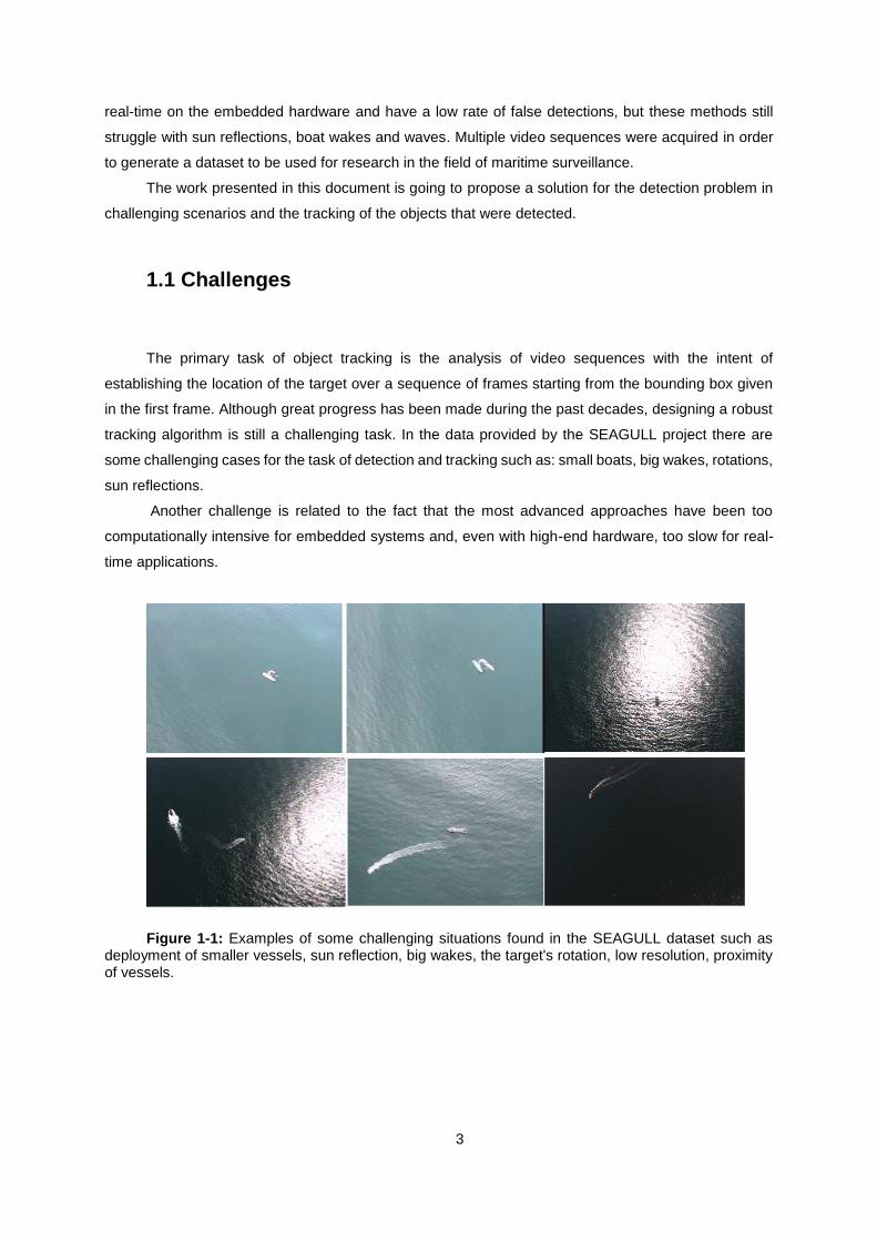
Figure 1-1: Examples of some challenging situations found in the SEAGULL dataset such as

deployment of smaller vessels, sun reflection, big wakes, the target's rotation, low resolution, proximity

of vessels. ................................................................................................................................................ 3

Figure 3-1: Outlines of the implementation used throughout the work. ..................................... 17

Figure 3-2: Scheme of the SSD architecture from (Liu et al. 2016) work. Used to illustrate the

architecture and layers of the Single Shot detector. ............................................................................. 18

Figure 3-3: Architecture of the CFNN (Yang Li et al.) Tracker pipeline. .................................... 19

Figure 3-5: Example of a ground truth in XML format. ............................................................... 25

Figure 4-1: Evaluation of the precision according to OBT's benchmark of both tracker models.

With the Threshold being the Location error threshold, in pixels. According to OBT's benchmark the

precision of the model corresponds to the value of precision of the threshold of 20. ........................... 35

Figure 4-2: The drift of the tracker, mostly due to the rotation of the vessel. In green the proposed

bounding box of the tracker. In red, the ground truth box corresponding to this frame ........................ 36

Figure 4-3: The tracker has a small drift due to the movement of the ship, in a more challenging

scenario, including bigger wakes. ......................................................................................................... 36

Figure 4-4: A image of the first (right) and last (left) frame of the image sequence of

smallBoatMoving ................................................................................................................................... 37

Figure 4-5: An example of a successful detection and a false positive ..................................... 38

Figure 4-6: An example of two false positives and a failed detection ........................................ 38

x

List of Tables

Table 4-1: Specifications of the computer used to run the experiments of this methodology of

detection and tracking in the maritime scenario. The specifications of the hardware used are detailed

and the version of the software applied. ................................................................................................ 30

Table 4-2: Number of Positive and Negative Samples in the Train and in the Test set ............. 32

Table 4-3: Composition of the training set, including the name of the video, the number of positive

and the number of negative samples .................................................................................................... 32

Table 4-4: Composition of the validation set, including the name of the video, the number of

positive samples and the number of negative samples. ....................................................................... 33

xi

List of Acronyms

ASLAS Coarse and Fine Structural Local Sparse Appearance Model

BB Bounding Box

CFNN Correlation Filter Neural Network

CNN Convolutional Neural Network

CPU Central Processing Unit

KCF Kernalized Correlation Filter

DNN Deep Neural Network

GPU Graphical Processing unit

GT Ground Truth

HOG Histogram of Gradients

IVT Incremental Learning for Robust Visual Tracking

mAP Mean Average Precision

MIL Multiple Instances Learning

MOSSE Minimum Output Sum of Squared Error

NN Neural Network

PCA Principal Component Analysis

R-CNN Region-Based Convolutional Neural Networks

RoI Region of Interest

RPN Region Proposal Network

SCM Sparse Collaborative Appearance Model

SPP Spatial Pyramid Pooling

SSD Single Shot Detector

STRUK Structured Output Tracking with Kernels

SVM Support Vector Machine

TLD Tracking-Learning-Detection

UAV Unmanned Aerial Vehicle

VOC Visual Object Challenge

VOT Visual Object Tracking

YOLO You Only Look Once

YOLT You Only Look Twice

xii

1

1. Introduction

Contents

1. Introduction ................................................................................................................................ 1

1.1 Motivation ............................................................................. Erro! Marcador não definido.

1.2 Challenges .......................................................................................................................... 3

1.3 Objectives ............................................................................................................................ 4

1.4 Contributions ....................................................................................................................... 4

1.5 Outlines ............................................................................................................................... 4

2

Object tracking is a very relevant problem in computer vision for its many applications, for

example: human computer interaction, maritime surveillance, traffic monitoring and driverless vehicles

(Djukic 2017).

With the migrant crisis that Europe has been facing since 2015 (Migrant crisis: Migration to Europe

2016), maritime surveillance has become a matter of international interest. That interest also is related

to some aviation disasters in sea areas that require the location of the wreckage and many other

applications.

Frontex (Mathiason et al. 2015) (FRONTEX - European Border and Coast Guard Agency), the

European agency that manages the cooperation between national borders' authorities securing

Europe's external borders, struggles with lack of equipment and human resources to perform a proper

surveillance of large portions of the sea. Still, the evolution of technology provides efficient and

alternative solutions such as the use of unmanned patrols.

Since Portugal has the third largest Exclusive Economic Zone within the European Union and one

of the largest in the world (Portugal - Exclusive Economic Zone - EEZ) it is very important that the country

invests in the surveillance of such a vast maritime territory. The 1,727,408 km² of Portugal's Exclusive

Economic Zone require an efficient surveillance system. The kind of interventions that the Portuguese

Air Force has to handle in the maritime surveillance can be subdivided into:

• detection and control of illegal activity;

• illegal immigration;

• detection of maritime pollution;

• control of maritime traffic;

• military operations;

• search and rescue missions;

• control of fishing activities.

The most used methods in the maritime surveillance of the Portuguese coastal area are based

in coastal radars, vessel-positioning systems, alarm systems, remote sensing and manned aircraft

patrols. Manned patrols are limited in terms of speed and area that can be monitored and require lots

of investment. So, having drones that are capable of detecting and tracking boats and ships in maritime

environment is a major advantage that should be further explored, since it is economically more viable

and there's an increasing need of surveillance in maritime scenarios.

The SEAGULL project (Monteiro Marques et al.) develops an affordable and intelligent maritime

surveillance system using Unmanned Aerial Vehicles (UAVs) equipped with optical sensors of several

types (visible, infrared, multi- and hyper-spectral). This system is a great example of the advantages of

unmanned maritime surveillance since it is easy to deploy and doesn't have many infrastructure

requirements.

A fleet of fixed wing UAVs is equipped with computers running vision algorithms for the automatic

detection of maritime vessels. After the vehicle is detected, its coordinates are transmitted to a coastal

ground station through a radio link. The algorithms (S. Marques et al. 2014) used in the project work in

3

real-time on the embedded hardware and have a low rate of false detections, but these methods still

struggle with sun reflections, boat wakes and waves. Multiple video sequences were acquired in order

to generate a dataset to be used for research in the field of maritime surveillance.

The work presented in this document is going to propose a solution for the detection problem in

challenging scenarios and the tracking of the objects that were detected.

1.1 Challenges

The primary task of object tracking is the analysis of video sequences with the intent of

establishing the location of the target over a sequence of frames starting from the bounding box given

in the first frame. Although great progress has been made during the past decades, designing a robust

tracking algorithm is still a challenging task. In the data provided by the SEAGULL project there are

some challenging cases for the task of detection and tracking such as: small boats, big wakes, rotations,

sun reflections.

Another challenge is related to the fact that the most advanced approaches have been too

computationally intensive for embedded systems and, even with high-end hardware, too slow for real-

time applications.

Figure 1-1: Examples of some challenging situations found in the SEAGULL dataset such as deployment of smaller vessels, sun reflection, big wakes, the target's rotation, low resolution, proximity of vessels.

4

1.2 Objectives

The goal of this work is to provide a system of detection of maritime vessels in maritime scenarios

and proceed to track them throughout the image sequence, adopting methods that correspond to the

current state-of-the-art approaches in object detection and tracking. The chosen approaches require the

least possible amount of computing power, due to the limitations of the workstation in use.

The trained network for object detection must be as accurate as possible in order to detect the

vessels even in challenging situations and the tracking process must be done the closest possible to

real time without compromising accuracy.

1.3 Contributions

The contributions of this work are:

• the training of a Single Shot Detector model with the provided data of the SEAGULL

dataset in the MATLAB convolutional neural networks’ library, MatConvNet;

• The implementation of a Sparse Correlation Filter Neural Network for tracking and the

comparison of the results to the model proposed in (Yang Li et al. 2017)The Sparse approach is

based on (Yanmei Dong et al. 2016).

• Tools to convert data from the SEAGULL dataset format to the standard PASCAL VOC

format: XML annotations, a tool to identify the images that are positive for a certain category, in

this case: boat or background.

• Tools to convert from video to image sequence.

• Renaming tools so that the filenames correspond to the PASCAL VOC format.

• Provided suggestions of correction for the MatConvNet implementation of the Single

Shot Detector.

1.4 Outline

This work is organized as follows. In Chapter 2 we present the current state-of-the-art tracking

algorithms and detection algorithms, including a few existing applications to maritime scenarios. Then,

in Chapter 3 we present the methodology behind the proposed approach and its main components: the

correlation filter tracker and the deep neural network detection algorithm the conditions in which the

work was carried are also mentioned in this chapter. In Chapter 4 we give an overview of the evaluations

5

performed. Finally, Chapter 5 summarizes the main conclusions of this work and refers to directions for

future research.

6

2. Related Work

Contents

2 Related Work ……………………………………………………………………………….…………..6

2.1 Deep Neural Network for Object Detection .......................... Erro! Marcador não definido.

2.1.1 Region-Based Convolutional Neural Networks (R-CNNs)Erro! Marcador não

definido.

2.1.2 Spatial Pyramid Pooling (SPP) ..................................... Erro! Marcador não definido.

2.1.3 Fast R-CNN ................................................................... Erro! Marcador não definido.

2.1.4 Faster R-CNN ................................................................ Erro! Marcador não definido.

2.1.5 You Only Look Once (YOLO) ........................................ Erro! Marcador não definido.

2.1.6 Single Shot Detector (SSD) .......................................... Erro! Marcador não definido.

2.2 Visual Object Tracker ........................................................... Erro! Marcador não definido.

2.2.1 Incremental Learning for Robust Visual Tracking ......... Erro! Marcador não definido.

2.2.2 Multiple Instance Learning (MIL) ................................... Erro! Marcador não definido.

2.2.3 Tracking-Learning-Detection (TLD)............................... Erro! Marcador não definido.

2.2.4 Robust Object Tracking via Sparse Collaborative Appearance Model (SCM) ...... Erro!

Marcador não definido.

2.2.5 Visual Tracking via Coarse and Fine Structural Local Sparse Appearance Model

(ASLAS) ............................................................................................ Erro! Marcador não definido.

2.2.6 Structured Output Tracking with Kernels (STRUK) ....... Erro! Marcador não definido.

2.2.7 High-Speed Tracking with Kernelized Correlation FiltersErro! Marcador não

definido.

2.2.8 Correlation Filter Neural Network (CFNN) .................... Erro! Marcador não definido.

2.2.9 Correlation Filter Tracker .............................................. Erro! Marcador não definido.

2.2.10 Convolutional Neural Network Tracker ....................... Erro! Marcador não definido.

7

2.3 Detection and Tracking in the Maritime Scenario ................ Erro! Marcador não definido.

Neural Networks have been a relevant topic nowadays. Its applications are wide spread, and its

importance is growing in our world. Throughout this section, some of the major breakthroughs that were

published related to the topic of object detection and object tracking are going to be presented. The

evolution of the algorithms, their limitations and how they were surpassed.

2.1 Deep Neural Network for Object Detection

Deep Neural Networks (DNNs) (Christian Szegedy et al.) have recently shown an outstanding

performance on the image classification tasks. As we achieve a deeper understanding of images and

Neural Networks (NNs) it is becoming necessary not only to classify but also precisely localize objects

of various classes.

The object detection consists on classifying images, but also accurately estimating the class and

location of objects contained within an image.

Major advances were possible due to an improvement in machine learning models and in object

representations.

Shallow discriminatively trained models in conjunction with manually engineered representations

have been standing as the paradigm of the best performing algorithms for object detection. Recently,

DNNs have emerged as a powerful machine learning model. The latter have deeper architectures which

have the capacity to learn more complex models than the shallow ones. To increase the performance,

it was needed to manage to detect objects with different scales. To solve that problem a pyramid of

images (Adelson et al. 1984) with different scales is generated by scaling the input image. The goal of

this approach is to guarantee that no matter the size of our window, the object will be contained in it.

Usually the image is down sampled until a certain minimum size. On each and every one of these levels

a fixed size window detector is run (Christian Szegedy et al.). All these windows are fed to a classifier

to detect the object of interest, this way, the scale problem and the location problem are solved.

2.1.1 Region-Based Convolutional Neural Networks (R-CNNs)

After the development of DNN classifiers, that proved to be better-performing, more accurate

classifiers than the HOG feature-based classifiers, it was expected that the later would be replaced.

However, the computational cost of the Neural Networks (NNs) and its speed were its major problems.

Running a CNN in every patch generated by the sliding window detector was impossible. To solve that

problem, R-CNN uses Selective Search (J.R.R. Uijlings, K.E.A. van de Sande, T. Gevers 2012) as the

proposed algorithm. Selective Search reduced the number of bounding boxes fed to the classifier to

8

about 2000 region proposals. To generate these region proposals Selective Search resorts to local

features such as texture, color, intensity, etc. decreasing the amount of information fed to the CNN-

based classifier reduces complexity and running time. All the generated boxes must be resized before

entering the fully-connected part of the CNN. The R-CNN can be summarized in four major parts:

• Run the Selective Search to generate region proposals Regions of Interest (RoI);

• Use the RoIs as input of the CNN;

• Feed the CNN output to the SVM to predict the object classes;

• Optimize the process by training the bounding box regression separately.

2.1.2 Spatial Pyramid Pooling (SPP)

Running a CNN in, approximately, 2000 RoIs takes a lot of time, which makes R-CNN very slow.

SPP (Kaiming He et al. 2014) was proposed as a way to overcome R-CNN’s limitations. SPP creates a

CNN representation of the image once and uses that to compute the CNN representation of each of

Selective Search’s regions. That is possible by doing a pooling operation only in the section of the

feature map of the last convolutional layer. To calculate the location of the RoI in the last layer it is

necessary to project the region in the convolutional layer, so it is necessary to take into account the

down sampling that happens in the middle layers.

SPP uses a spatial pyramid pooling layer after the last convolutional layer, instead of the most

common max-pooling. This is done to ensure that the size of the input of the fully connected layers is

fixed. In this layer, a region of arbitrary size is divided into a constant number of bins and the max pooling

operation is done to each and every one of these bins. Since the number of bins remains the same, the

produced vector has a constant size.

SPP’s major drawback was the difficulty of preforming back propagation through the spatial

pooling layers, so it only fine-tunes the fully connected layers.

2.1.3 Fast R-CNN

The Fast R-CNN (Girshick 2015) proposes a way to propagate the gradients through spatial

pooling, allowing it to overcome SPP’s limitations. A simple back-propagation calculation, very similar

to max-pooling gradient calculation, is done in regions that overlap so a cell can have gradients pumping

in from various regions.

Fast R-CNN implements Bounding Box (BB) regression to the neural network training itself. This

served for a multitask purpose of the network: the regression head and the classification head. The

classification head outputs the scores of each class and the regression head outputs the coordinates of

the proposed bounding box. This allows that the training of the network to work both for classification

9

and localization, increasing its speed. Its performance is better than SPP because the whole network is

trained instead of just a part of it.

2.1.4 Faster R-CNN

Faster R-CNN (Ren et al. 2015) , one of the most accurate object detection algorithms, replaced

the slowest part of Fast R-CNN, the Selective Search with a small convolutional network called Region

Proposal Network (RPN) to generate the RoI, allowing its faster performance.

Faster R-CNN also introduces the idea of anchor boxes, to deal with variations of scale and

aspect ratios of the objects. Three kinds of anchor boxes (128x128, 256x256, 512x512), for scale, and

three aspect ratios (1:1, 2:1, 1:2) are used at each location. So, at each location RPN predicts the

probability of being background or foreground in 9 different boxes. Bounding box regression is

implemented to provide better anchor boxes. RPN outputs bounding boxes of various sizes with the

corresponding probability of the object being of a certain class. With Spatial Pooling, as used in Fast R-

CNN, bounding boxes of different sizes can be passed further. The rest of the network is similar to Fast

R-CNN but, approximately 10 times faster.

2.1.5 You Only Look Once (YOLO)

Instead of approaching object detection as a classification problem where there is a pipeline in

which regions of interest are generated and then proceed to a classification/regression head, YOLO

(Redmon et al. 2016) treats object detection as a simple regression problem. For this regression problem

YOLO takes as input the image and learns the class probabilities and bounding box coordinates.

YOLO divides an image into a S x S grid, each of these grids predict N bounding boxes and

confidence (accuracy of the bounding box and whether or not the box actually contains an object). A

score for every class in training is also predicted for each of the S x S x N boxes. With these scores it is

possible to calculate the probability of each class being present in a certain box. The boxes with low

confidence can be removed. The threshold of the confidence can be changed, changing also the number

of boxes that remain. YOLO only predicts one class in one grid at once, so small objects are its

limitations. The whole image is seen at once instead of looking for region proposals, with this contextual

information, false positives are avoided. This algorithm can be run real time.

If main goal of the object detection is reducing computational time, YOLO presents the quickest

solution between the presented alternatives.

2.1.6 Single Shot Detector (SSD)

10

SSD (Liu et al. 2016) is a good algorithm in terms of accuracy and speed. The convolutional

network is run only once on the input image and a feature map is calculated. Then, a small convolutional

kernel runs on the feature map to predict bounding boxes at various aspect ratios (like Faster R-CNN

does) and instead of learning the bounding box it focuses on learning the boxes’ off-set. SSD predicts

bounding boxes after the convolutional layers to handle scale, since each convolutional layer operates

at a different scale, multiple scales can be detected.

SSD is less computationally demanding and achieves good results.

2.2 Visual Object Tracker

Visual tracking is one of the main challenges for the computer vision community, for its multiple

applications in real life such as surveillance, navigation, traffic control, augmented reality, etc. Even

though nowadays is possible to find algorithms for object tracking with a good performance, it is still

hard to develop a robust and efficient tracker due to background clutter, partial occlusion, motion blur,

etc. When it comes to the relevant application of this work, the vessel tracking, there are some specific

challenges. Some of these challenges are the variation in illumination, the rotations either from the

vessels or from the UAV itself, and some of the challenges already mentioned above.

In recent years the tracking algorithms presented at the Visual Object Tracking (VOT) challenge

that had the better results in the competition were based on correlation filter trackers.

2.2.1 Incremental Learning for Robust Visual Tracking

Incremental Learning for Robust Visual Tracking (IVT) (Ross et al. 2008) developed in 2008, was

a huge milestone in visual object tracking. Its counterparts used only appearance data available before

the beginning of the tracking operation. This ignored a large volume of information (such as illumination

changes or changes in shapes) that becomes available during tracking. So, IVT presented an algorithm

that efficiently adapts to changes in appearance of the target by incrementally learning a low-

dimensional subspace representation. The update of the model is done based on incremental algorithms

for Principal Component Analysis (PCA). Two important features distinguished this update: a method

for correctly updating the sample mean, and a forgetting factor to guarantee that less modeling power

is expended in trying to fit older observations. Both of these features allowed a measurably improvement

in the tracking performance, even in environments in which the target suffers from large changes in

scale, pose, illumination.

11

2.2.2 Multiple Instance Learning (MIL)

Unlike other methods that employ static appearance models that can be defined manually or

trained using the first frame and struggle to track objects that change in appearance throughout the

image sequence, MIL (Babenko et al. 2011) adaptative model that evolves during the tracking process

as the object’s appearance changes. This led to a tracker with better performance. MIL also models the

background and feeds it to a discriminative classifier. This approach is often called “tracking by

detection”, for its principle is very similar to object detection.

Multiple Instance Learning is a learning paradigm that claims that during training, examples are

presented in sets (named “bags”) and labels are provided for the bags instead of individual instance. If

a bag has at least one positive instance, it is labeled as positive, otherwise the bag is considered

negative. The learning algorithm has to distinguish from all the instances in a bag labeled as positive

the one that is the most correct.

With this approach a more robust tracker was achieved.

2.2.3 Tracking-Learning-Detection (TLD)

When we want to apply a tracking algorithm to an image sequence, in which the objects suffer

from occlusion or are not always visible, we are facing a long-term tracking problem. Some methods

address this as a detection problem with the inconvenience that object detectors are more

computationally demanding than its tracker counterparts, that only require initialization, are fast and

produce smooth trajectories. Trackers, however, accumulate errors throughout the run time (drift) and

when the object is not visible they tend to fail.

TLD’s (Kalal et al. 2012) goal is to decompose long-term tracking into three separate parts:

Tracking, Learning, and Detection. The tracker follows the object from frame to frame. The detector

localizes the object and corrects the tracker, if necessary. The other innovation that TLD brought to the

table was the P-N learning that evaluates the detector in every frame. P-expert is responsible for

recognizing missed detections and N-expert is responsible for recognizing false alarms. Both work

together in order to retrain the detector and avoid future errors. All three components run at the same

time and in real time.

2.2.4 Robust Object Tracking via Sparse Collaborative Appearance Model

(SCM)

12

An object can be represented by multiple characteristics such as texture, color, intensity, and

more. The representative schemes can be local histograms or holistic templates. SCM (Zhong et al.

2014) use intensity values to represent the objects because it is an efficient and simple approach. SCM

also relies on the strength of holistic templates to distinguish the foreground (target) from the background

and local patches to handle partial occlusion.

SCM is a robust tracker that proposes a collaboration between a generative model (in which

tracking is formulated as searching for the most similar region to the object being tracked within its

neighborhood) and a discriminative classifier (that treats tracking as a binary classification problem that

intends to design a classifier to distinguish the target from the background). This collaboration results in

a flexible method in which the model is adaptively updated considering appearance changes and

minimizing drifts.

2.2.5 Visual Tracking via Coarse and Fine Structural Local Sparse

Appearance Model (ASLAS)

ASLAS (Jia et al. 2016) proposes a tracking algorithm based on coarse and fine structural local

sparse models. Taking advantage of the fact that local appearance remains approximately constant

over time while the global appearance changes.

The algorithm computes sparse codes of local patches by averaging and performing an alignment

pooling to model the appearance of the object for visual tracking. For robust representation a novel

algorithm for constructing coarse and fine dictionaries is presented. To register the appearance changes

of the objects a template update scheme based on incremental subspace learning is implemented. The

template update scheme has an occlusion detection module to include pixels belonging to foreground

objects. A vast number of tests has been performed on this model to assure its performance.

2.2.6 Structured Output Tracking with Kernels (STRUK)

STRUK (Hare et al. 2016) presents a different approach from the traditional adaptive tracking-by-

detection paradigm. STRUK pointed out that tracking-by-detection models have two inconveniences:

one is that it was unclear how to generate and label the samples in a principled way. The second is that

the learning process does not explicitly couple the classifier’s goal (predict labels) to the tracker’s

(estimate the object’s location). So, these two parts can induce errors in the classifier since the

confidence levels cannot be appropriate to the tracking function.

STRUK predicts the change in the object configuration between frames. For that tracking and

learning are integrated, excluding the need of ad-hoc update strategies. STRUK has no offline labelled

data available for training other than object’s location on the first frame and relies only in online learning.

To avoid excessive computational cost, the online learning of classification SVMs is kept limited.

13

2.2.7 High-Speed Tracking with Kernelized Correlation Filters

The discriminative learning methods are widespread in which from an initial image patch

containing the target the model is supposed to learn a classifier to distinguish the target’s appearance

and the background. Each new image is another patch to update the model. Instinctively it makes sense

to focus on the samples of the object, the positive samples. But the core of the discriminative methods

is to emphasize the negative samples, the background. The negative samples are image patches from

different locations and scales, so there is an infinite number of possible negatives. For this reason, there

is a need to compromise the number of negative samples incorporated and the desired speed of the

algorithm. It follows that, the usual practice is to randomly choose a few samples from each frame.

KCF (Henriques et al. 2015) presents a tool to incorporate thousands of samples at different

relative translations without explicitly iterating over them. This tool is called circulant matrixes. KCF is a

tracker based on Kernel Ridge Regression that does not suffer from the asymptotic complexity of other

kernelization methods. It even exhibits lower complexity than unstructured linear regression. It is a

kernelized version of a linear correlation filter, which is the base from today’s fastest trackers.

2.2.8 Correlation Filter Neural Network (CFNN)

Deep learning has been demonstrating the best results in most of the computer vision

applications. So, Convolutional Neural Networks (CNNs) were integrated in an increasing amount of

works of object tracking. But the training process requires many videos and annotated data, which

makes it a very time-consuming task.

The Correlation Filters operation is similar to the deep learning operation in the sense that both

of them try to find the best suitable filter to distinguish foreground from background. The correlation filter-

based method quickly learns a model from a single frame without need of previous training process.

The Correlation Filter Neural Network (CFNN) (Yang Li et al. 2017) integrates the advantages of

both tracking methods: it follows the typical deep learning tracker’s framework without requiring any pre-

training. This is possible by densely sampling the first frame with circulant matrix and applying a ridge

regression to estimate the model for the network. The model is then integrated into a two-layer CNN

structure and CFNN initialized.

The network outputs a target location probability map (in which the highest probability

corresponds to the new location of the target) that can be used to collect negative samples. This allows

the network to selectively update the model. When reaching a certain interval (every 7 frames), the

collected frames along the way are backpropagated to tune the CFNN. This updates the weights

adaptatively to the variation of appearance.

14

2.2.9 Correlation Filter Tracker

Filter learning was formulated by (Bolme et al. 2010) as a regression problem which estimates

the filter through cost minimization accordingly to samples from the first frame. The work of (Henriques

et al. 2015) shows that dense sampling with circulant matrixes and Histogram of Gradients (HOG)

features with the kernel trick (Navneet Dalal and Bill Triggs 2005) leads to better results. Other

extensions of correlation filter-based tracking were proposed. Some cope with scale estimation, others

propose an interpolation method to merge convolutional maps from multiple layers in order to obtain

much reliable response map. The current state-of-the-art approaches are all based in Correlation Filter

Trackers.

In the 2017 Visual Object Tracking (VOT) competition (Matej Kristan et al. 2017) the winner used

an approach of Convolutional Features for Correlation Filters. In a competition where real-time tracking

was one of the most relevant criteria to evaluate the proposed methods.

The idea of the correlation filters is to produce a peak in the location of the object that is supposed

to be tracked and a low result in the background. Correlation filters are very effective, but until the

proposal of the Minimum Output Sum of Squared Error (MOSSE) filter, there was not a viable way to

preform online tracking. From the MOSSE developments arise, for example, the Kernalized Correlation

Filters (KCF) (Yang Li et al. 2017) that consisted in introducing kernel methods to the tracker. The KCF

uses multi-channel Histogram of Oriented Gradients (HOG) features instead of the raw image pixels

used by MOSSE.

Correlation filter-based trackers obtain the correlation result by employing dot-product in

frequency domain, in time domain, this corresponds to circulant padding around the original search

window. Unnecessary boundary effects might be introduced by a large area of circulant padding since

the template has the same size as the search window.

Hard negative sampling is also used in CFNN to integrate the most important information from

previous frames, leading to better results.

2.2.10 Convolutional Neural Network Tracker

The trackers that use CNN-based methods need to extract good features to get a fair

representation of the target. Some approaches train a pre-built target model, before tracking. Others

emphasize on feature representation with Convolutional Neural Networks in which the discrimination

between object and background is performed by a classification layer. Another used approach is to use

a lower layer and a top layer of a pre-trained network. As it has been previously explained, the lower

layer and a top layer have two different representations of the same object, so it is easier to discard

noise or feature maps that are unrelated to the target. Some approaches require an offline training of

15

the network, even though this approach requires a large number of labeled videos and images. This

kind of network can be used to track various targets without the need of online updating.

CFNN (Yang Li et al. 2017) relies on discriminative classification without performing any pre-

training on an external dataset. As was mentioned above, CFNN has a two-layer CNN architecture so

that the model can be trained efficiently with samples from the first frame.

Another relevant feature of the CFNN (Yang Li et al. 2017) is the fact that it requires no fixed-size

input and output. So, the model is able to extend the searching area to arbitrary sizes.

2.3 Detection and Tracking in the Maritime Scenario

A vast work has been done when it comes to visual object detection and tracking, although very

few methods address the problem in the maritime scenario. The detectors that use a sliding window and

HOG features struggle with non-uniform background. Illumination changes, the motion of the UAV, the

wakes and waves, the in-plane and out-of-plane rotations that would be inexistent in a motionless

camera are challenges that our problem encounters. You Only Look Twice (YOLT) is a method

conceived specially for vessel and airplane multi-scale detection with satellite imagery in maritime and

harbor/airport environments. Using airborne image sequences increases the challenge due to the

movement of the UAV’s maneuvers besides the challenges already indicated concerning the maritime

scenario.

In this work is combined a state-of-the-art detector to a Kernelized Correlation Filter Tracker to

achieve accurate detection and precise tracking.

The current state-of-the-art approaches try to make it possible for real-time analysis, that is,

minimizing the computational cost without compromising the accuracy obtained. Areas with sun

reflections, waves and wakes and rotations in the movement are usually a cause of fail in many of the

trackers built for general purpose. On longer sequences, as well, some drift is experienced. Key point

trackers are not a viable option for the analyzed scenario since there’s a lack of texture and low-

resolution targets.

In this work an integration of the output of a trained SSD network will be presented and having

the detected bounding box becoming the input of the KCF which will run in the rest of the image

sequence.

16

3. Methodology

Contents

3 Methodology …………………………………………………………………………………………..16

3.1 Architecture ....................................................................................................................... 17

3.2 Single Shot Detector ......................................................................................................... 18

3.3 Tracker .............................................................................................................................. 19

3.3.1 Architecture ................................................................................................................ 19

3.3.2 Weights Initialization and Update ............................................................................... 20

3.3.3 Tracking Framework .................................................................................................. 23

3.4 Training of the Detector ..................................................................................................... 24

3.4.1 Data Treatment .......................................................................................................... 24

3.4.2 Matching Strategy ...................................................................................................... 26

3.4.3 Training Objective ...................................................................................................... 26

3.4.4 Scales and Aspect Ratios for default Bounding Boxes .............................................. 27

17

3.4.5 Hard Negative Mining ................................................................................................. 27

3.4.6 Data Augmentation .................................................................................................... 28

3.1 Architecture

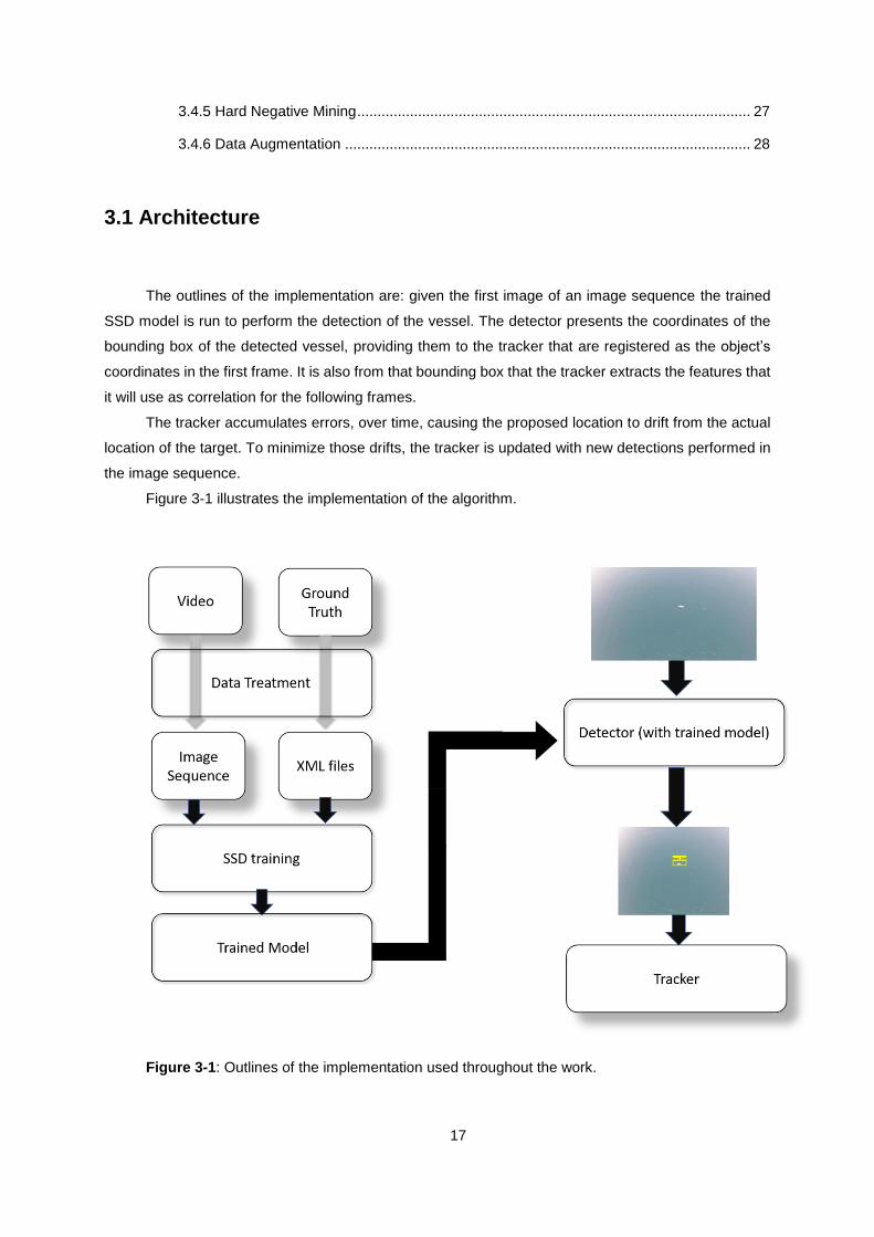
The outlines of the implementation are: given the first image of an image sequence the trained

SSD model is run to perform the detection of the vessel. The detector presents the coordinates of the

bounding box of the detected vessel, providing them to the tracker that are registered as the object’s

coordinates in the first frame. It is also from that bounding box that the tracker extracts the features that

it will use as correlation for the following frames.

The tracker accumulates errors, over time, causing the proposed location to drift from the actual

location of the target. To minimize those drifts, the tracker is updated with new detections performed in

the image sequence.

Figure 3-1 illustrates the implementation of the algorithm.

Figure 3-1: Outlines of the implementation used throughout the work.

18

3.2 Single Shot Detector

Single Shot Detector (Liu et al. 2016) is currently the state-of-the-art approach for object detection.

It is based on a different paradigm than its other competitors that are based on variants of: hypothesizing

bounding boxes, resampling pixels or features for each box, and apply a high-quality classifier. The SSD

has prevailed on detection benchmarks since the Selective Search work (J.R.R. Uijlings, K.E.A. van de

Sande, T. Gevers 2012) through the current leading results on PASCAL VOC, COCO, and ILSVRC

detection all based on Faster R-CNN (Ren et al. 2015). While accurate, these approaches have been

too computationally intensive for embedded systems and, even with high-end hardware, too slow for

real-time applications. Often detection speed for these approaches is measured in Frames Per Second

(FPS), and the fastest detectors, such as Faster R-CNN operate at 7 FPS. There have been several

attempts to build faster detectors by implementing new methods to different stages of the detection

pipeline, but so far, increasing the speed has compromised the accuracy of the detection.

SSD is the first detector that does not resamples pixels or features for bounding box (BB)

hypotheses and maintains the same levels of accuracy. The fundamental improvement in speed comes

from eliminating bounding box proposals and the subsequent pixel or feature resampling stage. The

improvements include using a small convolutional filter to predict object categories and offsets in

bounding box locations, using separate predictors (filters) for different aspect ratio detections, and

applying these filters to multiple feature maps from the later stages of a network to perform detection at

multiple scales. Mainly due to this step of detection at multi-scales, it is possible to obtain high-accuracy

using relatively low-resolution inputs leading to a faster detection

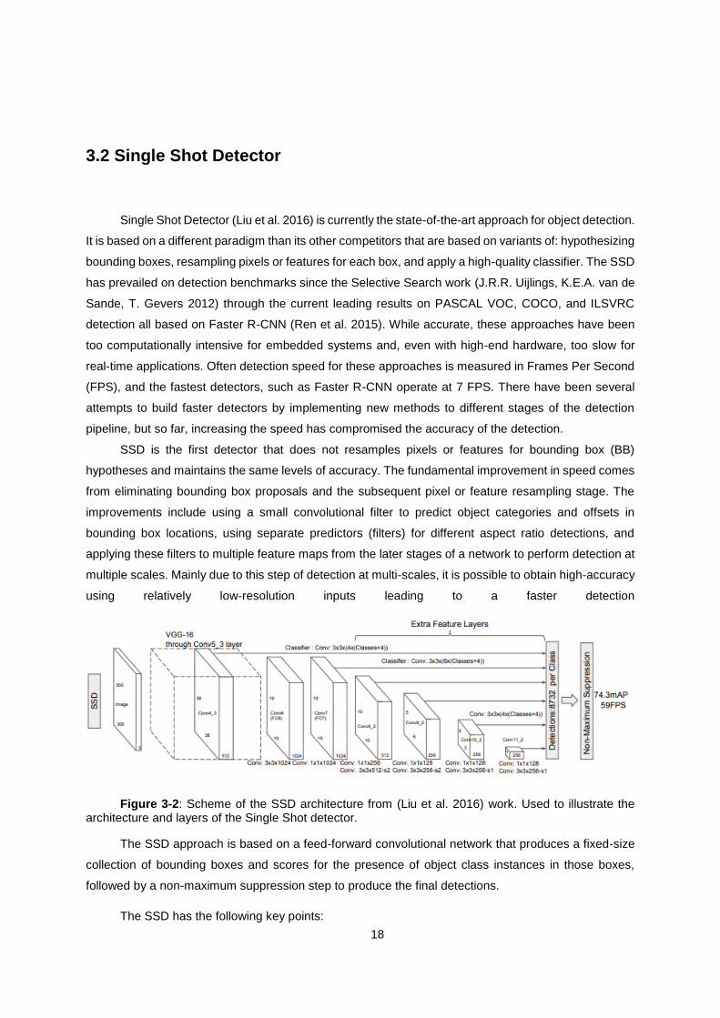
Figure 3-2: Scheme of the SSD architecture from (Liu et al. 2016) work. Used to illustrate the architecture and layers of the Single Shot detector.

The SSD approach is based on a feed-forward convolutional network that produces a fixed-size

collection of bounding boxes and scores for the presence of object class instances in those boxes,

followed by a non-maximum suppression step to produce the final detections.

The SSD has the following key points:

19

• SSD is faster than the previous state-of-the-art single shot detectors, YOLO (Redmon

et al. 2016) and is more accurate. As accurate as techniques that perform explicit region

proposals (like Faster R-CNN (Ren et al. 2015)).

• SSD predicts category scores and box offsets for a fixed set of default bounding boxes,

small convolutional filters are applied to the feature maps.

• Predictions are separated by aspect ratio and are produced at different scales for

feature maps of different scales, which makes SSD so accurate.

• Even in low-resolution input images the end-to-end training of a network with these

design features, provides a better compromise of speed vs accuracy.

3.3 Tracker

To find successive positions of an object throughout an image sequence we use a tracker system.

In this section, the architecture of the system used is described and the details concerning the

implementation are also referred. The adopted model is the sparse approach of the CFNN (Yang Li et

al. 2017).

3.3.1 Architecture

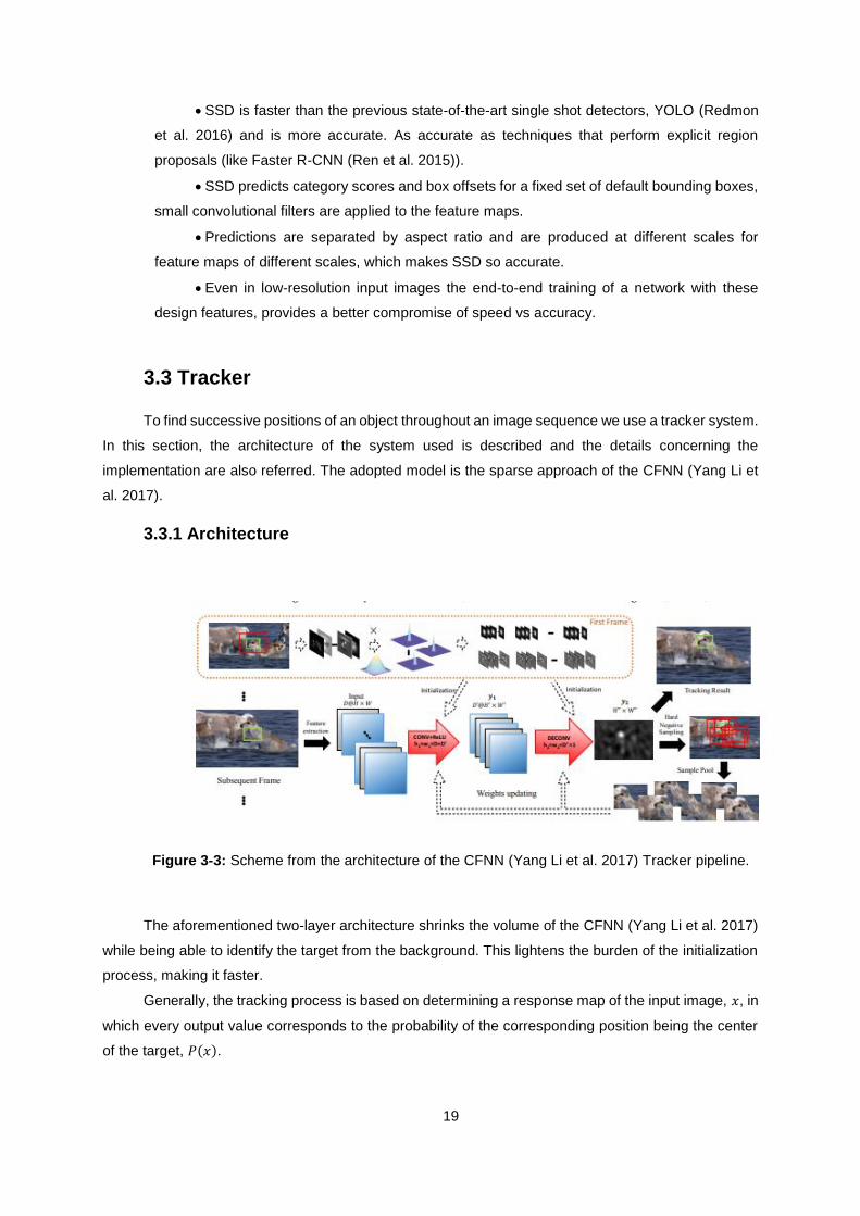
Figure 3-3: Scheme from the architecture of the CFNN (Yang Li et al. 2017) Tracker pipeline.

The aforementioned two-layer architecture shrinks the volume of the CFNN (Yang Li et al. 2017)

while being able to identify the target from the background. This lightens the burden of the initialization

process, making it faster.

Generally, the tracking process is based on determining a response map of the input image, 𝑥, in

which every output value corresponds to the probability of the corresponding position being the center

of the target, 𝑃(𝑥).

20

𝑃(𝑥) = 𝑓2 𝑜 𝑓1 (𝓕(𝒙)) (1)

In equation (1), 𝑓2 and 𝑓1 are the two convolutional layers of the CFNN. And ℱ(𝑥) is the feature

extraction operator, that extracts the features from input image, 𝑥. 𝑓1 obtains the response maps with

multiple filters. Each ℱ(𝑥) ∈ ℝ𝐻𝑥𝑊𝑥𝑁, has 𝑁 channels, in 𝑓1, 𝑁′ filters are created (𝑊1 =

𝑊11, 𝑊1

2, … , 𝑊1𝑁′

). These filters perform the convolution with the input features. After the convolution

operation, the first layer output map is given by: 𝑦1 = 𝑓1(ℱ(𝑥)) ⊂ ℝ𝐻′𝑥𝑊′𝑥𝑁′ in which 𝑦1

𝑖 = 𝑓1𝑖 =

𝜎(ℱ(𝑥) ⊗ 𝑤1𝑖 + 𝑏1

𝑖 ) that corresponds to the ReLU activation function of the convolution between the

extracted features and its corresponding weights (𝑤1𝑖) and bias (𝑏1

𝑖 ). The weights have the following

format: 𝑤1 ∊ ℝℎ1𝑥 𝑤1 𝑥 𝑁 𝑥𝑁′, where ℎ1𝑥 𝑤1 correspond to the kernel size.

The second layer, 𝑓2, merges 𝑦1𝑖 , the response maps from 𝑓1 in a reasonable way and exploits

the deconvolution to increase the resolution of the final response map. 𝑓2’s weights have the format:

𝑤2 ∊ ℝℎ2𝑥 𝑤2 𝑥 𝑁′𝑥 1, with a fractional stride. The deconvolution performed by 𝑓2 yields 𝑦2. With 𝑦2 being:

𝑦2 ∊ ℝ𝐻′′𝑥𝑊′′𝑥 1(𝐻′′ > 𝐻′ and 𝑊′′ > 𝑊′) and so the final probability map from CFNN is described. The

weights on both layers are trained from the samples that the algorithm takes from every input image.

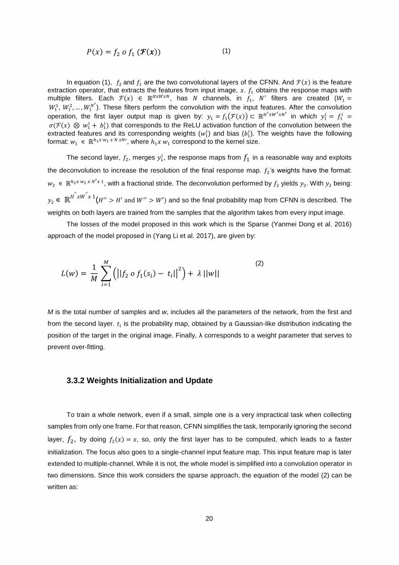
The losses of the model proposed in this work which is the Sparse (Yanmei Dong et al. 2016)

approach of the model proposed in (Yang Li et al. 2017), are given by:

𝐿(𝑤) = 1

𝑀 ∑ (||𝑓2 𝑜 𝑓1(𝑠𝑖) − 𝑡𝑖||

2) + 𝜆 ||𝑤||

𝑀

𝑖=1

(2)

M is the total number of samples and w, includes all the parameters of the network, from the first and

from the second layer. 𝑡𝑖 is the probability map, obtained by a Gaussian-like distribution indicating the

position of the target in the original image. Finally, λ corresponds to a weight parameter that serves to

prevent over-fitting.

3.3.2 Weights Initialization and Update

To train a whole network, even if a small, simple one is a very impractical task when collecting

samples from only one frame. For that reason, CFNN simplifies the task, temporarily ignoring the second

layer, 𝑓2, by doing 𝑓2(𝑥) = 𝑥, so, only the first layer has to be computed, which leads to a faster

initialization. The focus also goes to a single-channel input feature map. This input feature map is later

extended to multiple-channel. While it is not, the whole model is simplified into a convolution operator in

two dimensions. Since this work considers the sparse approach, the equation of the model (2) can be

written as:

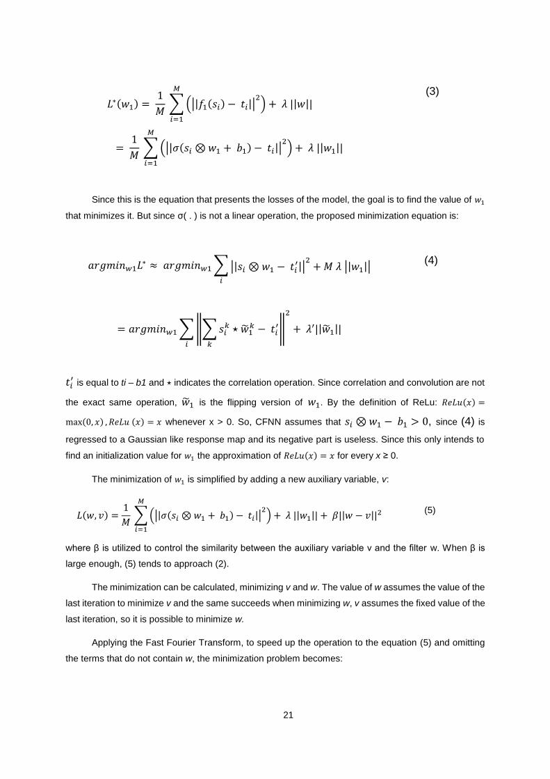
21

𝐿∗(𝑤1) = 1

𝑀 ∑ (||𝑓1(𝑠𝑖) − 𝑡𝑖||

2) + 𝜆 ||𝑤||

𝑀

𝑖=1

(3)

= 1

𝑀 ∑ (||𝜎(𝑠𝑖 ⊗ 𝑤1 + 𝑏1) − 𝑡𝑖||

2) + 𝜆 ||𝑤1||

𝑀

𝑖=1

Since this is the equation that presents the losses of the model, the goal is to find the value of 𝑤1

that minimizes it. But since σ( . ) is not a linear operation, the proposed minimization equation is:

𝑎𝑟𝑔𝑚𝑖𝑛𝑤1𝐿∗ ≈ 𝑎𝑟𝑔𝑚𝑖𝑛𝑤1 ∑ ||𝑠𝑖 ⊗ 𝑤1 − 𝑡𝑖′||

2+ 𝑀 𝜆 ||𝑤1||

𝑖

(4)

= 𝑎𝑟𝑔𝑚𝑖𝑛𝑤1 ∑ ‖∑ 𝑠𝑖𝑘 ⋆ �̃�1

𝑘 − 𝑡𝑖′

𝑘

‖

2

+ 𝜆′||�̃�1||

𝑖

𝑡𝑖′ is equal to ti – b1 and ⋆ indicates the correlation operation. Since correlation and convolution are not

the exact same operation, �̃�1 is the flipping version of 𝑤1. By the definition of ReLu: 𝑅𝑒𝐿𝑢(𝑥) =

max(0, 𝑥) , 𝑅𝑒𝐿𝑢 (𝑥) = 𝑥 whenever x > 0. So, CFNN assumes that 𝑠𝑖 ⊗ 𝑤1 − 𝑏1 > 0, since (4) is

regressed to a Gaussian like response map and its negative part is useless. Since this only intends to

find an initialization value for 𝑤1 the approximation of 𝑅𝑒𝐿𝑢(𝑥) = 𝑥 for every x ≥ 0.

The minimization of 𝑤1 is simplified by adding a new auxiliary variable, v:

𝐿(𝑤, 𝑣) =1

𝑀 ∑ (||𝜎(𝑠𝑖 ⊗ 𝑤1 + 𝑏1) − 𝑡𝑖||

2) + 𝜆 ||𝑤1||

𝑀

𝑖=1

+ 𝛽||𝑤 − 𝑣||2

(5)

where β is utilized to control the similarity between the auxiliary variable v and the filter w. When β is

large enough, (5) tends to approach (2).

The minimization can be calculated, minimizing v and w. The value of w assumes the value of the

last iteration to minimize v and the same succeeds when minimizing w, v assumes the fixed value of the

last iteration, so it is possible to minimize w.

Applying the Fast Fourier Transform, to speed up the operation to the equation (5) and omitting

the terms that do not contain w, the minimization problem becomes:

22

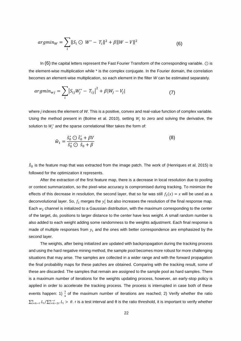
𝑎𝑟𝑔𝑚𝑖𝑛𝑊 = ∑‖𝑆𝑖 ⊙ 𝑊∗ − 𝑇𝑖‖2 + 𝛽‖𝑊 − 𝑉‖2

𝑖

(6)

In (6) the capital letters represent the Fast Fourier Transform of the corresponding variable. ⊙ is

the element-wise multiplication while * is the complex conjugate. In the Fourier domain, the correlation

becomes an element-wise multiplication, so each element in the filter W can be estimated separately.

𝑎𝑟𝑔𝑚𝑖𝑛𝑤𝑗 = ∑|𝑆𝑖𝑗𝑊𝑗∗ − 𝑇𝑖𝑗|

2+ 𝛽|𝑊𝑗 − 𝑉𝑗|

𝑖

(7)

where j indexes the element of W. This is a positive, convex and real-value function of complex variable.

Using the method present in (Bolme et al. 2010), setting 𝑊𝑗 to zero and solving the derivative, the

solution to 𝑊𝑗∗ and the sparse correlational filter takes the form of:

�̂�1 =�̂�0

∗ ⊙ �̂�0′ + 𝛽𝑉

�̂�0∗ ⊙ �̂�0 + 𝛽

(8)

�̂�0 is the feature map that was extracted from the image patch. The work of (Henriques et al. 2015) is

followed for the optimization it represents.

After the extraction of the first feature map, there is a decrease in local resolution due to pooling

or context summarization, so the pixel-wise accuracy is compromised during tracking. To minimize the

effects of this decrease in resolution, the second layer, that so far was still 𝑓2(𝑥) = 𝑥 will be used as a

deconvolutional layer. So, 𝑓2 merges the 𝑦1𝑖 but also increases the resolution of the final response map.

Each 𝑤2 channel is initialized to a Gaussian distribution, with the maximum corresponding to the center

of the target, do, positions to larger distance to the center have less weight. A small random number is

also added to each weight adding some randomness to the weights adjustment. Each final response is

made of multiple responses from 𝑦1 and the ones with better correspondence are emphasized by the

second layer.

The weights, after being initialized are updated with backpropagation during the tracking process

and using the hard negative mining method, the sample pool becomes more robust for more challenging

situations that may arise. The samples are collected in a wider range and with the forward propagation

the final probability maps for these patches are obtained. Comparing with the tracking result, some of

these are discarded. The samples that remain are assigned to the sample pool as hard samples. There

is a maximum number of iterations for the weights updating process, however, an early-stop policy is

applied in order to accelerate the tracking process. The process is interrupted in case both of these

events happen: 1) 3

4 of the maximum number of iterations are reached; 2) Verify whether the ratio

∑ 𝐿𝑖𝑛𝑖=𝑛−𝑟 ∑ 𝐿𝑖

𝑛−𝑟𝑖=𝑛−2𝑟 > 𝜃⁄ . r is a test interval and θ is the ratio threshold, it is important to verify whether

23

the last iterations are relevant and if there is the need to iterate more. The ratio is set up to 0.98 (Yang

Li et al. 2017).

When the cost from one iteration to the next has an extreme increase (the values are diverging),

the learning rate is adjusted to a smaller one in attempt to find convergence. If he cost of the current

network is higher than a threshold, when comparing to the last iteration, the current network is regarded

as an exception. The handling measures for these exceptions are: 1) discard of all the weights

modifications in the iteration to the weights of the previous iterations; 2) The decrease of the learning

rate. Once the learning rate decreases, it is constantly updated in every iteration until it reaches the

default value of 0.0003.

This flexibility in the learning rate creates robustness and ensures that even in more challenging

scenarios the network can adapt itself.

3.3.3 Tracking Framework

CFNN’s tracking system localizes the target for the location that scores the maximum confidence

with the probability maps mentioned in (1). The location of the center of the target is determined by:

𝑧 = 𝑎𝑟𝑔𝑚𝑎𝑥𝑧 ∊ 𝑥𝑃(�̃�|𝑐) (9)

where x defines a searching space with potential candidates and c corresponds to the priori constraint,

that is extracted from all the previous frames. c, is embedded in the weights of the previous network

since the weights are adjusted with samples from the previous frames. The tracking process is a forward

propagation. This means that for any position in a search window, the location of the target can be

obtained by passing its surrounding patch into the system as Equation

A search window is cropped to locate the target before tracking around the bounding box of the

target from the previous frame. Then, a feature map is generated from the search window due to the

extraction of proper features and multiplication of a Hann window with it.

The manipulated feature map becomes the input of the two-layer convolutional neural network.

The tracking on the following frames is performed by forward propagation and predicts the position of

the target. During the tracking process a set of samples is collected from every frame and their labels

are generated based on predictions as well. The weights of the CNN are updated every frame interval

(in the case of this work, every 7 frames) to take appearance variations into account.

24

3.4 Training of the Detector

In this section a detailed description of the process of training the Single Shot Detector Network

will be provided, including details on the format of the input data. Some tools that were developed during

this work are presented here.

3.4.1 Data Treatment

To facilitate the training of the Single Shot Detector network, a standard data format is adopted.

PASCAL VOC format was adopted as it is a standard and it is common to find auxiliary material and

code for this format. PASCAL VOC format consists of the videos converted to image sequences, and

the ground truths in XML file format

The provided dataset consists of videos acquired at a frame rate of 25 Frames Per Second (FPS),

where each frame has 1920x1080 pixels. Each video has a corresponding text file with annotations. The

given annotations have the format: <frame number> <top left x> <top left y> <width> <height>

<object id>. The frame number corresponds to the frame number in the sequence of video. The top

left x and top left y represent the position, in pixels, of the top left corner of the bounding box. The y

axis points downwards and the x axis points from left to right. The width and height correspond to the

size of the bounding box, in pixels, in the horizontal and vertical axis, respectively. The object id is used

to distinguish objects in video sequences in which there are multiple objects. A label consists of the

minimum sized rectangular area that contains an object.

The XML file (Figure 3-4) is hierarchically constructed, it has a root node, in this case is the

Annotation node. The Annotation node has the following child nodes: Folder, Filename, Source, Size

and Object.

The Folder indicates the path of the image this annotation corresponds to. The Filename

corresponds to the name of the image that has this annotation, every frame that has at least one object

has a corresponding annotation. The frames that do not contain objects are annotated as background.

The Source has a child node called Database to indicate from which dataset the image belongs to.

Other parameters can be added such as the author of the image or, if it is an image available online,

provide a link. It is basically where the credits can be found. The Size node corresponds to the size of

the image. In the SEAGULL dataset, has we have mentioned before, all the images have the same size:

a width of 1920 pixels by a height of 1080 pixels, the depth corresponds to the number of color

channels in the image, since all these are color images, they have three color channels: Red, Green

and Blue (RGB). A grayscale image would have only one in depth. Finally, the Object node includes all

the information that corresponds to the bounding box information and labels. The name contains the

class of the object, in this case we only have the class ‘boat’ or ‘background’. The pose provides

information concerning the orientation of the object in the image (vertical, horizontal, unspecified...). The

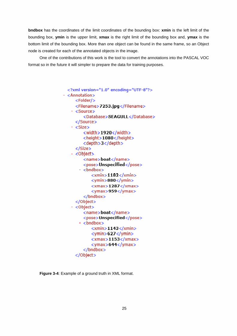
25

bndbox has the coordinates of the limit coordinates of the bounding box: xmin is the left limit of the

bounding box, ymin is the upper limit, xmax is the right limit of the bounding box and, ymax is the

bottom limit of the bounding box. More than one object can be found in the same frame, so an Object

node is created for each of the annotated objects in the image.

One of the contributions of this work is the tool to convert the annotations into the PASCAL VOC

format so in the future it will simpler to prepare the data for training purposes.

Figure 3-4: Example of a ground truth in XML format.

26

3.4.2 Matching Strategy

It is necessary to determine which default bounding boxes correspond to a ground truth detection,

so that it is possible to properly train the network. Each ground truth box is matched to the default

bounding boxes (that vary in location, aspect ratio and scale) which presents the best jaccard overlap

(10). A match occurs when the default bounding boxes have a jaccard overlap superior to 0.5 with the

ground truth bounding boxes. Multiple overlapping default boxes can be obtained instead of picking only

the one with maximum overlap, which simplifies the learning process.

𝐽(𝐴, 𝐵) =|𝐴 ∩ 𝐵|

|𝐴 ∪ 𝐵|

(10)

3.4.3 Training Objective

In SSD there is a derivation of the MultiBox training objective (minimization of the losses), in the

original model, it is extended for multiple object categories, however, in this work, this is not the case.

𝑥𝑖𝑗𝑝

= {0, 1} is an indicator to match the i-th default box to the j-th ground truth box, of category, p. The

matching strategy is described as ∑ 𝑥𝑖𝑗𝑝

𝑖 ≥ 1. The overall loss of the model is a weighted sum of the

localization loss (loc_loss) and the confidence loss (conf_loss). The overall loss is given by:

𝐿(𝑥, 𝑐, 𝑙, 𝑔) =1

𝑁(𝐿𝑐𝑜𝑛𝑓(𝑥, 𝑐) + 𝛼 𝐿𝑙𝑜𝑐(𝑥, 𝑙, 𝑔))

(11)

N corresponds to the number of matched default boxes. The loss is set to 0, in the case that no default

box was matched (N = 0) and the weight of α set to 1 by cross-validation. The localization loss is a

Smooth L1 loss between the parameters of the predicted box (l) and the ground truth box (g). Like in

Faster R-CNN (Ren et al. 2015), SSD regresses to offsets for the center (cx, cy) of the default bounding

box (d) and its width (w) and height (h).

Localization loss is given by:

𝐿𝑙𝑜𝑐(𝑥, 𝑙, 𝑔) = ∑ ∑ 𝑥𝑖𝑗𝑘 𝑠𝑚𝑜𝑜𝑡ℎ𝐿1(𝑙𝑖

𝑚 − �̂�𝑗𝑚

𝑚 ∊{𝑐𝑥,𝑐𝑦,𝑤,ℎ}

)

𝑁

𝑖 ∊𝑃𝑜𝑠

(12)

27

�̂�𝑗𝑐𝑥 =

(𝑔𝑗𝑐𝑥 − 𝑑𝑖

𝑐𝑥)𝑑𝑖

𝑤⁄ �̂�𝑗𝑐𝑦

=(𝑔𝑗

𝑐𝑦− 𝑑𝑖

𝑐𝑦)

𝑑𝑖ℎ⁄

�̂�𝑗𝑤 = log (

𝑔𝑗𝑤

𝑑𝑖𝑤) �̂�𝑗

ℎ = log (𝑔𝑗

ℎ

𝑑𝑖ℎ)

And, finally, the confidence loss is the softmax loss over multiple classes confidences (c) and is

given by:

𝐿𝑐𝑜𝑛𝑓(𝑥, 𝑙, 𝑔) = − ∑ 𝑥𝑖𝑗𝑝 log(�̂�𝑖

𝑝) − ∑ log (�̂�𝑖0)

𝑖 ∊ 𝑁𝑒𝑔

𝑁

𝑖 ∊𝑃𝑜𝑠

(13)

where, �̂�𝑖𝑝

= exp(𝑐𝑖

𝑝)

∑ exp(𝑐𝑖𝑝

)𝑝

3.4.4 Scales and Aspect Ratios for default Bounding Boxes

Some methods such as SPP (Kaiming He et al. 2014), suggest that processing the image at

different sizes and combining the results afterwards is the best way to handle different object scales.

However, SSD uses feature maps from several different layers in a single network for prediction to mimic

the same effect. Some parameters are also shared across all object scales.

In the work of (Long et al. 2016) it is shown that using feature maps from lower layers can improve

semantic segmentation quality (feature maps from different levels from the same network have different

receptive field sizes). This happens since lower layers capture more fine details of the input objects.

Plus, it provides a global context pooling from a feature maps smooths the results.

SSD uses the lower and upper feature map for detection. By combining the predictions for all

default boxes with scales (that can vary from 0.2 up to 0.9) and aspect ratios (that can be one of the

following {1, 2, 3, 1

2,

1

3}) from all the locations of many feature maps, the obtained set of predictions

covers multiple sizes and shapes for the input object.

3.4.5 Hard Negative Mining

After the matching process, most of the boxes left are not matched to ground truth boxes, this

means that they are negatives. There is an imbalance in the number of the positive and the negative

28

samples, so SSD sorts the samples using the highest confidence loss for each default box. The top

ones are picked so that the ratio of negative-to-positive samples is 3:1.

3.4.6 Data Augmentation

Data Augmentation is used to make the model more robust whether it is for different input sizes,

shapes. Each image in the training is randomly sampled by one of three different options:

• Use the entire original input image;

• Sampling a patch so that the minimum jaccard overlap with the object’s bounding box

is 0.1; 0.3; 0.5; 0.7; or 0.9.

• Randomly sample a patch - the size of the patch is from 0.1 up to 1 of the size of the

original images and the aspect ratio between 1 2⁄ and 2. The overlapped part of the ground truth

box is kept as long as its center is in the sampled patch. After the sampling step, the sampled

patches are resized to fixed size and is horizontally flipped with a probability of 0.5, in addition,

some photo-metric distortions are applied similarly to the one used by (Andrew G. Howard

2013).

Throughout this work data augmentation was used since in (Liu et al. 2016) they conclude that

data augmentation leads to better results. Also, since the dataset was split, we considered that it would

be fruitful to use this tool.

29

4. Experimental Results

and Setup

Contents

4 Experimental Results and Setup …………………………………………………………………...29

4.1 Workstation ....................................................................................................................... 30

4.2 Tracker Evaluation ............................................................................................................ 30

4.3 Detector Evaluation ........................................................................................................... 31

4.4 Limitations ......................................................................................................................... 31

4.5 Data ................................................................................................................................... 31

4.6 Training Setup ................................................................................................................... 33

4.7 Results Obtained ............................................................................................................... 34

4.8 SSD Training ..................................................................................................................... 37

30

In this chapter the experimental conditions are presented as well as some of the results obtained

with the setup described. The workstation, evaluation metrics, data used, the setup of the training

process as well as examples of the results obtained can be found throughout this chapter.

4.1 Workstation

The proposed method is computationally expensive (both in processing time and memory

requirements), even though the choice of the algorithms took into account the computation needed to

perform the task. The processing time was one of the major constraints found in this work. All the

processing done within this work was performed with CPU computation only.

The computer specifications of the workspace used to run the experiments are presented in the

following Table 4-1.

Table 4-1: Specifications of the computer used to run the experiments of this methodology of detection and tracking in the maritime scenario. The specifications of the hardware used are detailed and the version of the software applied.

Processor Intel® Core™ i7-7700 CPU @ 3.60 GHz

Graphics Card Intel ® HD Graphics 630

RAM Memory 16,0 Gb (15,9 Gb usable)

Operating System Windows 10 Pro

MATLAB version R2016a

MatConvNet 1.0-beta25

Microsoft Visual Studio 2015 Community Edition

4.2 Tracker Evaluation

For the tracking process the evaluation metric we follow the metric of precision of the Object

Tracking Benchmark (Wu et al. 2013) . The Precision metric is based in the center location error. Center

location error is defined as the Euclidean distance between the center locations of the tracked target

and the center of the labeled ground truth (manually labeled). Previous metrics averaged over the center

location error and used that to summarize the performance of the tracker. When the target is lost, the

tracker’s output location is usually random, compromising the average of the center location.

In this work, the percentage of frames whose estimated location error is bellow a given threshold.

The possible threshold values go from 0 to 50 with a step of 1 pixel. According to (Wu et al. 2013) the

percentage that is chosen to rank the tracker corresponds to a threshold of 20 pixels.

31

4.3 Detector Evaluation

The metric used to evaluate the trained network is the mean average precision (mAP). Mean

average precision is an extension of the average precision. The average of all average precisions is

taken to calculate the mAP. The mean average precision, for a certain class is given by:

𝑚𝐴𝑃 = ∑ 𝐴𝑣𝑒𝑟𝑎𝑔𝑒 𝑃𝑟𝑒𝑐𝑖𝑠𝑖𝑜𝑛(𝑖)𝑇

𝑖=1

𝑁(𝑐𝑙𝑎𝑠𝑠𝑒𝑠)

(14)

4.4 Limitations

Mostly due to hardware limitations, the amount of experiments done throughout this work was not

the desired. There are some experiments that were not possible to concretize due to the amount of time

they would require, such as the training of the network with the full dataset, since the expected amount

of time was of 72 days. So, some compromises were made. The compromises made were:

• Instead of training the Single Shot Detector Network with a dataset of, approximately, 70.000

images, we trained 2 batches of 700 images each and 100 images to test.

• The tracking process was evaluated on fragments of the image sequence of 450 images per

video.

• Experiments with small targets were tried but not evaluated since the average time per frame

was 10 minutes.

• Other tracking or detection methods were not tested, so the comparison will be done with the

results of the original methods.

4.5 Data

Single Shot Detector (Liu et al. 2016)has a hard negative mining training strategy. This consists

of keeping a 3:1 ratio of negative-to-positive samples. This strategy is used because keeping this ratio

leads to a faster optimization and a more stable training. So, overall, we provide 3 times more negative

samples than positive ones.

32

The data is split into 2 different parts: the training set, that has approximately 70% of the annotated

data and the validation set, with, approximately 30%. In each of this sets the negative-to-positive ratio

is kept 3:1, in Table 4-1 is the distribution of the images per set:

Table 4-2: Number of Positive and Negative Samples in the Train and in the Test set

Train Validation

Number of Images 55 176 20 696

Positives 13 794 6 455

Negatives 41382 14 241

The composition of the sets is indicated in the Table 4-3 and Table 4-4.

Table 4-3: Composition of the training set, including the name of the video, the number of positive and the number of negative samples

Train

Video name Positives Negatives

bigShipHighAlt_clip1 1 276 -

bigShipHighAlt_clip2 1 921 330

GP020175_part_02 1 080 -

GP050027_part01 696 24

GP030175_part01 4 610 250

GP050027_part02 183 1 257

Gp050027_part04 358 122

GP060027_part00 378 42

lanchaArgos_clip2 942 129

lanchaArgos_clip3 1 239 162

smallBoatStopped 1 122 1 129

GP020175_part00 - 11 880

GP030027 - 11 400

GP040027_part04 - 1 560

GP040173 - 13 260

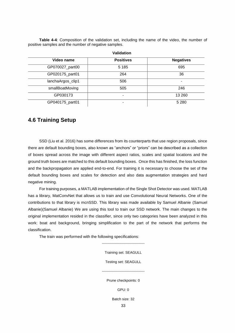
33

Table 4-4: Composition of the validation set, including the name of the video, the number of positive samples and the number of negative samples.

Validation

Video name Positives Negatives

GP070027_part00 5 185 695

GP020175_part01 264 36

lanchaArgos_clip1 506 -

smallBoatMoving 505 246

GP030173 - 13 260

GP040175_part01 - 5 280

4.6 Training Setup

SSD (Liu et al. 2016) has some differences from its counterparts that use region proposals, since

there are default bounding boxes, also known as “anchors” or “priors” can be described as a collection

of boxes spread across the image with different aspect ratios, scales and spatial locations and the

ground truth boxes are matched to this default bounding boxes. Once this has finished, the loss function

and the backpropagation are applied end-to-end. For training it is necessary to choose the set of the

default bounding boxes and scales for detection and also data augmentation strategies and hard

negative mining.

For training purposes, a MATLAB implementation of the Single Shot Detector was used. MATLAB

has a library, MatConvNet that allows us to train and use Convolutional Neural Networks. One of the

contributions to that library is mcnSSD. This library was made available by Samuel Albanie (Samuel

Albanie)(Samuel Albanie) We are using this tool to train our SSD network. The main changes to the

original implementation resided in the classifier, since only two categories have been analyzed in this

work: boat and background, bringing simplification to the part of the network that performs the

classification.

The train was performed with the following specifications:

------------------------------------

Training set: SEAGULL

Testing set: SEAGULL

------------------------------------

Prune checkpoints: 0

GPU: 0

Batch size: 32

34

------------------------------------

Train + val: 0

Flip: 0

Patches: 0

Zoom: 0

Distort: 1

------------------------------------

Learning Rate Schedule:

1e-03 (warmup)

3e-04 for 73 epochs

1e-05 for 35 epochs

The data provided for training was divided in several batches of, approximately 800 images each,

so that the train could finish (the whole training set would require about 72 days to be completed). The

training was run in smaller batches. After the training process is complete, an SSD trained model is

obtained which will be used to perform the detection of vessels in another image sequence.

4.7 Results Obtained

For an experiment ran with the same image sequence our model achieved better results than the

ones obtained with CFNN (Yang Li et al. 2017).

The cost of every iteration was reduced almost 10 times and the same happened to the losses.

Another point in favor of the proposed tracking model is that it runs faster than CFNN.

We’ll present the results obtained for the same image sequence, with 450 frames, the boat

present in every frame, no wakes or sun reflection:

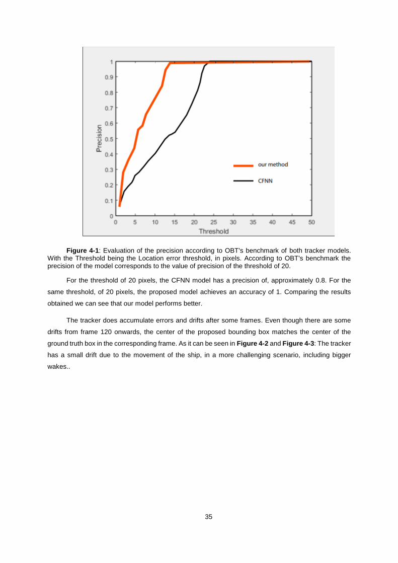
35

Figure 4-1: Evaluation of the precision according to OBT's benchmark of both tracker models. With the Threshold being the Location error threshold, in pixels. According to OBT's benchmark the precision of the model corresponds to the value of precision of the threshold of 20.

For the threshold of 20 pixels, the CFNN model has a precision of, approximately 0.8. For the

same threshold, of 20 pixels, the proposed model achieves an accuracy of 1. Comparing the results

obtained we can see that our model performs better.

The tracker does accumulate errors and drifts after some frames. Even though there are some

drifts from frame 120 onwards, the center of the proposed bounding box matches the center of the

ground truth box in the corresponding frame. As it can be seen in Figure 4-2 and Figure 4-3: The tracker

has a small drift due to the movement of the ship, in a more challenging scenario, including bigger

wakes..

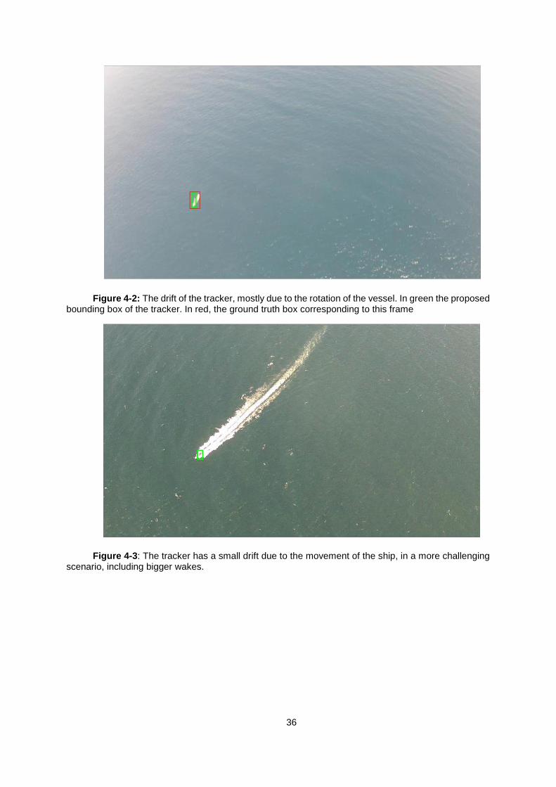
36

Figure 4-2: The drift of the tracker, mostly due to the rotation of the vessel. In green the proposed bounding box of the tracker. In red, the ground truth box corresponding to this frame

Figure 4-3: The tracker has a small drift due to the movement of the ship, in a more challenging scenario, including bigger wakes.

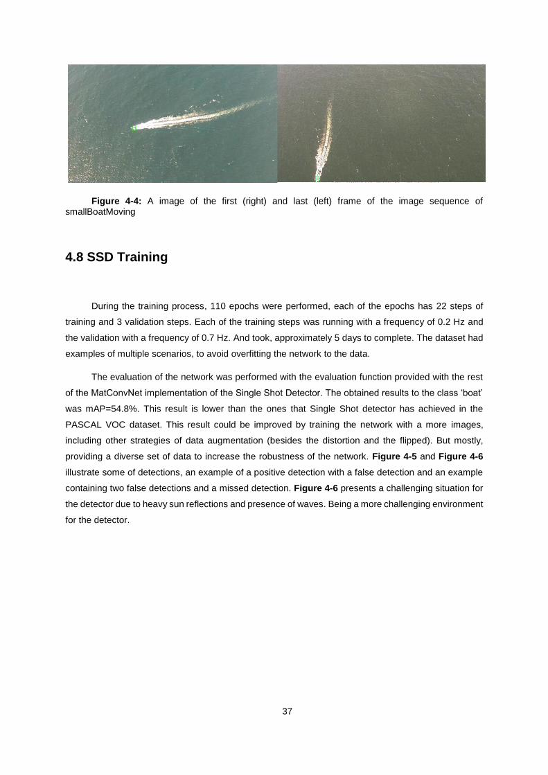
37

Figure 4-4: A image of the first (right) and last (left) frame of the image sequence of smallBoatMoving

4.8 SSD Training

During the training process, 110 epochs were performed, each of the epochs has 22 steps of

training and 3 validation steps. Each of the training steps was running with a frequency of 0.2 Hz and

the validation with a frequency of 0.7 Hz. And took, approximately 5 days to complete. The dataset had

examples of multiple scenarios, to avoid overfitting the network to the data.

The evaluation of the network was performed with the evaluation function provided with the rest

of the MatConvNet implementation of the Single Shot Detector. The obtained results to the class ‘boat’

was mAP=54.8%. This result is lower than the ones that Single Shot detector has achieved in the

PASCAL VOC dataset. This result could be improved by training the network with a more images,

including other strategies of data augmentation (besides the distortion and the flipped). But mostly,

providing a diverse set of data to increase the robustness of the network. Figure 4-5 and Figure 4-6

illustrate some of detections, an example of a positive detection with a false detection and an example

containing two false detections and a missed detection. Figure 4-6 presents a challenging situation for

the detector due to heavy sun reflections and presence of waves. Being a more challenging environment

for the detector.

38

Figure 4-5: An example of a successful detection and a false positive

Figure 4-6: An example of two false positives and a failed detection

39

5. Conclusions

Content

5 Conclusions……………………………………………………………………………………………39

5.1 Discussion ......................................................................................................................... 40

5.2 Future Work………………………………………………………………………………………41

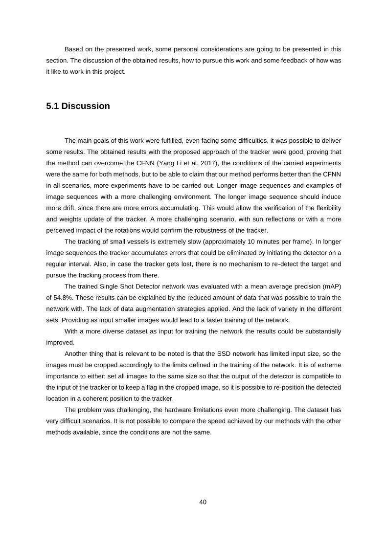
40

Based on the presented work, some personal considerations are going to be presented in this

section. The discussion of the obtained results, how to pursue this work and some feedback of how was

it like to work in this project.

5.1 Discussion

The main goals of this work were fulfilled, even facing some difficulties, it was possible to deliver

some results. The obtained results with the proposed approach of the tracker were good, proving that

the method can overcome the CFNN (Yang Li et al. 2017), the conditions of the carried experiments

were the same for both methods, but to be able to claim that our method performs better than the CFNN

in all scenarios, more experiments have to be carried out. Longer image sequences and examples of

image sequences with a more challenging environment. The longer image sequence should induce

more drift, since there are more errors accumulating. This would allow the verification of the flexibility

and weights update of the tracker. A more challenging scenario, with sun reflections or with a more

perceived impact of the rotations would confirm the robustness of the tracker.

The tracking of small vessels is extremely slow (approximately 10 minutes per frame). In longer

image sequences the tracker accumulates errors that could be eliminated by initiating the detector on a

regular interval. Also, in case the tracker gets lost, there is no mechanism to re-detect the target and

pursue the tracking process from there.

The trained Single Shot Detector network was evaluated with a mean average precision (mAP)

of 54.8%. These results can be explained by the reduced amount of data that was possible to train the

network with. The lack of data augmentation strategies applied. And the lack of variety in the different

sets. Providing as input smaller images would lead to a faster training of the network.

With a more diverse dataset as input for training the network the results could be substantially

improved.

Another thing that is relevant to be noted is that the SSD network has limited input size, so the

images must be cropped accordingly to the limits defined in the training of the network. It is of extreme

importance to either: set all images to the same size so that the output of the detector is compatible to

the input of the tracker or to keep a flag in the cropped image, so it is possible to re-position the detected

location in a coherent position to the tracker.

The problem was challenging, the hardware limitations even more challenging. The dataset has

very difficult scenarios. It is not possible to compare the speed achieved by our methods with the other

methods available, since the conditions are not the same.

41

5.2 Future Work

As future work, the training of the SSD network with a more complete set of data and exploring

further the different options and combinations of data augmentation strategies.

Conduct more experiments with the system proposed to perform the tracking process in larger

datasets and verify if its performance under different conditions.

Finally, the integration of the detection module and the tracking module. So, in case the tracker

gets lost it is possible to perform a detection action and re-locate the target.

42

6. Bibliography

Adelson, E. H.; Anderson, C. H.; Bergen, J. R.; Burt, P. J.; J. M. Ogden (1984): Pyramid Methods

in image processing.

Andrew G. Howard (2013): Some Improvements on Deep Convolutional Neural Network Based

Image Classification.

Babenko, Boris; Yang, Ming-Hsuan; Belongie, Serge (2011): Robust Object Tracking with Online

Multiple Instance Learning. In IEEE transactions on pattern analysis and machine intelligence 33 (8),

pp. 1619–1632. DOI: 10.1109/TPAMI.2010.226.

Bolme, David S.; Beveridge, J. Ross; Draper, Bruce A.; Lui, Yui Man (Eds.) (2010 - 2010): Visual

Object Tracking using Adaptive Correlation Filters. 2010 IEEE Conference on Computer Vision and

Pattern Recognition (CVPR). San Francisco, CA, USA, 13/06/2010 - 18/06/2010: IEEE.

Christian Szegedy; Alexander Toshev; Dumitru Erhan: Deep Neural Networks for Object

Detection.

Djukic, Bogdan (2017): Tracking cars and pedestrians from an autonomous vehicle. Available

online at https://medium.com/@bdjukic/tracking-cars-and-pedestrians-from-an-autonomous-vehicle-

ba1d2194b440.

FRONTEX - European Border and Coast Guard Agency. Available online at

https://frontex.europa.eu/.

Girshick, Ross (2015): Fast R-CNN.

Hare, Sam; Golodetz, Stuart; Saffari, Amir; Vineet, Vibhav; Cheng, Ming-Ming; Hicks, Stephen

L.; Torr, Philip H. S. (2016): Struck: Structured Output Tracking with Kernels. In IEEE transactions on

pattern analysis and machine intelligence 38 (10), pp. 2096–2109. DOI: 10.1109/TPAMI.2015.2509974.

Henriques, João F.; Caseiro, Rui; Martins, Pedro; Batista, Jorge (2015): High-Speed Tracking

with Kernelized Correlation Filters. In IEEE Trans. Pattern Anal. Mach. Intell. 37 (3), pp. 583–596. DOI:

10.1109/TPAMI.2014.2345390.

J.R.R. Uijlings, K.E.A. van de Sande, T. Gevers (2012): Selective Search for Object Recognition.

Jia, Xu; Lu, Huchuan; Yang, Ming-Hsuan (2016): Visual Tracking via Coarse and Fine Structural

Local Sparse Appearance Models. In IEEE transactions on image processing : a publication of the IEEE

Signal Processing Society 25 (10), pp. 4555–4564. DOI: 10.1109/TIP.2016.2592701.

Kaiming He; Xiangyu Zhang; Shaoqing Ren; Jian Sun (2014): Spatial Pyramid Pooling in Deep

Convolutional Networks for Visual Recognition.

43

Kalal, Zdenek; Mikolajczyk, Krystian; Matas, Jiri (2012): Tracking-Learning-Detection. In IEEE

transactions on pattern analysis and machine intelligence 34 (7), pp. 1409–1422. DOI:

10.1109/TPAMI.2011.239.

Liu, Wei; Anguelov, Dragomir; Erhan, Dumitru; Szegedy, Christian; Reed, Scott; Fu, Cheng-Yang;

Berg, Alexander C. (2016): SSD: Single Shot MultiBox Detector. In 0302-9743 9905, pp. 21–37. DOI:

10.1007/978-3-319-46448-0_2.

Long, Jonathan; Shelhamer, Evan; Darrel, Trevor (2016): Fully Convolutional Networks for

Semantic Segmentation.

Matej Kristan; Aleš Leonardis; Jiri Matas; Michael Felsberg; Roman Pflugfelder; Luka Čehovin

(2017): The Visual Object Tracking Challenge Results VOT2017.

Mathiason, Nick; Parsons, Victoria; Jeory, Ted (2015): Europe's refugee crisis: Is Frontex

bordering on chaos? Available online at http://labs.thebureauinvestigates.com/is-frontex-bordering-on-

chaos/.

Migrant crisis: Migration to Europe (2016). Available online at http://www.bbc.com/news/world-

europe-34131911.

Monteiro Marques, Mario; Dias, Pedro; Pessanha Santos, Nuno; Lobo, Victor; Batista, Ricardo;

Salgueiro, Diogo et al.: Oceans 2015 - Genova. 18 - 21 May 2015, Genova, Italy ; Oceans'15 MTS/IEEE

Genova Conference and Exhibit. Institute of Electrical and Electronics Engineers; Marine Technology

Society; Oceanic Engineering Society; Oceans MTS/IEEE Conference and Exhibit, Piscataway, NJ.

Available online at http://ieeexplore.ieee.org/servlet/opac?punumber=7227859.

Navneet Dalal and Bill Triggs (2005): Histograms of Oriented Gradients for Human Detection.

Portugal - Exclusive Economic Zone - EEZ. Available online at

https://www.globalsecurity.org/military/world/europe/pt-eez.htm.

Redmon, Joseph; Divvala, Santosh; Girshick, Ross; Farhadi, Ali (2016): You Only Look Once:

Unified, Real-Time Object Detection.

Ren, Shaoqing; He, Kaiming; Girshick, Ross; Sun, Jian (2015): Faster R-CNN: Towards Real-

Time Object Detection with Region Proposal Networks. Available online at

http://arxiv.org/pdf/1506.01497v3.

Ross, David A.; Lim, Jongwoo; Lin, Ruei-Sung; Yang, Ming-Hsuan (2008): Incremental Learning

for Robust Visual Tracking. In Int J Comput Vis 77 (1-3), pp. 125–141. DOI: 10.1007/s11263-007-0075-

7.

S. Marques, Jorge; Bernardino, Alexandre; Bento, Maria; Cruz, Gonçalo (2014): An algorithm for

the detection of vessels in aerial images.

Samuel Albanie: mcnSSD. A MatConvNet implementation of the Single Shot Detector.

44

Wu, Yi; Lim, Jongwoo; Yang, Ming-Hsuan (2013): Online Object Tracking: A Benchmark. In :

Online Object Tracking: A Benchmark. 2013 IEEE Conference on Computer Vision and Pattern

Recognition (CVPR). Portland, OR, USA, 23/06/2013: IEEE, pp. 2411–2418.

Yang Li; Zhan Xu; Jianke Zhu (2017): CFNN: Correlation Filter Neural Network for Visual Object

Tracking.

Yanmei Dong; Min Yang; Mingtao Pei (2016): VISUAL TRACKING WITH SPARSE

CORRELATION FILTERS, Image Processing (ICIP), 2016 IEEE International Conference Phoenix,

Arizona.

Zhong, Wei; Lu, Huchuan; Yang, Ming-Hsuan (2014): Robust object tracking via sparse

collaborative appearance model. In IEEE transactions on image processing : a publication of the IEEE

Signal Processing Society 23 (5), pp. 2356–2368. DOI: 10.1109/TIP.2014.2313227.