Detecting Jacobian sparsity patterns by Bayesian probinglennart/drgrad/Griewank2002.pdf ·...

Digital Object Identifier (DOI) 10.1007/s101070100281

Math. Program., Ser. A 93: 1–25 (2002)

Andreas Griewank · Christo Mitev

Detecting Jacobian sparsity patternsby Bayesian probing

Received: April 29, 2000 / Accepted: September 2001Published online April 12, 2002 – Springer-Verlag 2002

Abstract. In this paper we describe an automatic procedure for successively reducing the set of possiblenonzeros in a Jacobian matrix until eventually the exact sparsity pattern is obtained. The dependence in-formation needed in this probing process consist of “Boolean” Jacobian-vector products and possibly alsovector-Jacobian products, which can be evaluated exactly by automatic differentiation or approximated bydivided differences. The latter approach yields correct sparsity patterns, provided there is no exact cancellationat the current argument.

Starting from a user specified, or by default initialized, probability distribution the procedure suggestsa sequence of probing vectors. The resulting information is then used to update the probabilities that certainelements are nonzero according to Bayes’ law. The proposed probing procedure is found to require onlyO(log n) probing vectors on randomly generated matrices of dimension n, with a fixed number of nonzerosper row or column. This result has been proven for (block-) banded matrices, and for general sparsity patternfinite termination of the probing procedure can be guaranteed.

Key words. sparsity – automatic differentiation – difference quotients – conditional probability

1. Introduction and notation

Many numerical methods require the evaluation of Jacobians for vector functions givenas evaluation procedures. If known, the sparsity pattern of these first derivative matricescan be used to evaluate [CM84], store, and manipulate them more efficiently. Especiallyon discretizations of differential equations and other large scale problems, detectingand specifying the pattern of potentially nonzero entries may be a laborious and errorprone task. Therefore we investigate in this paper ways of determining the patternautomatically, without incurring the overhead of a dynamically sparse implementationof the chain rule like SparsLinC [BCK95].

1.1. Algorithmic differentiation background

Apart from computer algebra systems, which can be expected to work only for rathersmall problems, one may apply automatic, or algorithmic differentiation (AD) to con-veniently and reliably determine sparsity pattern. AD is based on the simple observationthat in the computational practice all functions are computed via a sequence of scalarassignments of the form

v = a(u, w) ≡ u ◦w or v = ϕ(u) . (1)

A. Griewank: Institute of Scientific Computing, Technical University Dresden, D-01062 Dresden,e-mail: [email protected]

C. Mitev: Treppenmeister GmbH, Emminger Straße 38, D-71131 Jettingen

2 Andreas Griewank, Christo Mitev

Here ◦ ∈ {+,−, ∗, /} represents an arithmetic operation and ϕ a univariate intrinsic likethe exponential or trigonometric functions. The partial derivatives au, aw and ϕu of allsuch elemental functions can be easily generated symbolically and then evaluated at thecurrent argument. The resulting floating point numbers can subsequently be combinedusing some version of the chain rule to yield the partial derivatives of all dependentvariables, denoted here by yi for i = 1 . . . m, with respect to all independent variables,denoted by x j for j = 1 . . .n (for details see [Gri00] and [CF+01]).

In the so-called forward mode of algorithmic differentiation one propagates inter-mediate gradients v ≡ ∇xv ≡ ∂v/∂x ∈ Rn according to the simple rules

v = au ∗ u + aw ∗ w and v = φu ∗ u . (2)

The resulting computational effort for evaluating y = F(x) and its Jacobian F′(x) =(∇ yT

i )i=1...m ∈ Rm×n with respect to x is bounded by a small multiple of n times theeffort of evaluating y by itself. Instead of propagating the full gradient vectors ∇xv

at once, one may restrict the chain rule application to the partials with respect to oneparticular independent variable so that in the recursions above v ≡ ∂v/∂x j ∈ R for somefixed j . The resulting partials yi for i = 1 . . . m then form the jth column of the Jacobianmatrix. One may also propagate partials with respect to a subset of p independents andthen obtains the corresponding p columns of the Jacobian at a time.

Since ∇x x j ≡ e j ∈ Rn is by definition a Cartesian basis vector, the gradients∇vx of intermediates v that occur early in the evaluation process tend to be rathersparse. Moreover, excluding incidental cancellations, sparsity must occur throughoutthe calculation if the Jacobian itself is sparse. The first AD tool that facilitates theautomatic detection and exploitation of Jacobian sparsity was the SparsLinC [BCK95]module of ADIFOR. It keeps all ∇xv in a sparse vector format, an approach that isvery flexible but incurs a significant runtime overhead at each new evaluation point(for specific runtimes see [BK+97]). Recently the packages ADOL-C [GJ+96] andTAMC [GK00] have acquired the capability to propagate the sparsity pattern

v ≡ (sign

∣∣∂v/∂x j∣∣)

j=1...n ∈ {0, 1}n

as bit-vectors. This approach avoids the manipulation of index sets and requires roughly1+ n/64 times as much storage and run-time as the original function itself, if the wholeJacobian sparsity pattern is to be evaluated at once. In this paper we aim to avoid theproportional dependence on n altogether by successively collecting and incorporatinginformation about the sparsity pattern. The factor 64 occurs assuming that the originalfunction evaluation is carried out in double precision reals, each of which takes as muchspace as two unsigned integers representing 32 bits. The bit patterns can be propagatedaccording to the rules

v = u | w or v = u (3)

which follow from (2) for au �= 0 �= aw or ϕu �= 0 with | representing a bitwise or.Again, the same recursions apply if the v and thus the v are restricted to a subset ofcomponents. In particular, if v is a pair of Boolean integers with 32 bits each, the bitwiseor (and of course mere copying) requires on modern computer chips only a couple ofmachine cycles, just like floating point additions and multiplications.

Detecting Jacobian sparsity patterns by Bayesian probing 3

In the study [GK01] it was found on the five problems FDC, FIC, IER, SFO, and SFIfrom the Minpack-2 test collection [AC+92] that propagating integers was never slowerand sometimes considerably faster than propagating doubles representing directionalderivatives. Therefore we assume throughout the paper, that at the cost of evaluatingone column of the Jacobian by forward automatic differentiation in double precisionarithmetic, one may determine the sparsity pattern of at least 64 columns by bit-patternpropagation. In the reverse mode, one obtains analogous results for the transpose, sothat one row of the Jacobian is about as expensive to obtain as the sparsity pattern of64 of them. Of course one can also propagate just one bit representing the dependenceon a single independent variable per intermediate value, either forward or backward.However, that won’t be much cheaper than doing 32 of them simultaneously in eithermode. In any case one should keep in mind, that either one of these efforts is a smallmultiple of the cost to evaluate the function y = F(x) by itself.

These basic observations regarding computational costs are the only results fromAD that are needed in the remainder of this paper. Moreover, our probing approachis also applicable to differencing, a simple technique that might be unavoidable, forexample when source code for evaluating the function is not available.

1.2. Sparsity patterns and Boolean probes

Throughout the paper we assume that some vector function

F ≡ (Fi)i=1...m : Rn �→ Rm

is continuously differentiable on some neighbourhood D of a given vector argumentx ≡ (x j) j=1...n ∈ Rn . Then we may define the sparsity pattern of the Jacobian

F′(x) ≡ ∂

∂xF(x) ∈ Rm×n

near x as the Boolean matrix S ≡ (si j )i=1...mj=1...n ∈ {0, 1}m×n with

si j = 0 ⇐⇒ ∂Fi(x)/∂x j ≡ 0 at all x ∈ DThe key assumption for the application of the techniques to be developed in this paperis the following. Given any vector t ∈ {0, 1}n we must be able to evaluate the Booleanvector r ≡ (ri)i=1...m ≡ S t ∈ {0, 1}m with

ri = 1 ⇐⇒ si j = 1 = t j for at least one j ≤ n . (4)

We will refer to the pair (t, r) or more generally to any other partial information thatwe can gather about the unknown matrix S as a “probe”. A related but different conceptof probing is used in domain decomposition methods to precondition matrices witha large number of very small entries (see [BSG96] and the original proposals [CP+74]and [NR83]).

The “Boolean product” r might be evaluated directly by propagating suitable de-pendence information through a given evaluation procedure for F, as sketched in the


previous Subsect. 1.1. If no AD software with this capability is available, one may baseour probing method on the following consequence of the mean value theorem

Fi(x) �= Fi(x + ε t) �⇒ ri = 1 . (5)

Here ε is assumed nonzero but small and t is interpreted as a real 0−1 vector in thiscontext. Unfortunately, the converse implication is not strictly true as the inequalityon the left may happen to be violated, yet ri may still be equal to 1. However, forgeneric x ∈ Rn and ε ∈ R such exact cancellations are extremely unlikely to occur, anddetermining the m components of r on the basis of the difference F(x + εt) − F(x) isprobably as safe as any other calculation one performs in floating point arithmetic. Ineither case, we will be able to detect sparsity exclusively on the basis of the qualitativedependence information represented by r as a function of t and possibly correspondingtranspose probes as defined below.

Apart from its greater reliability the key advantage of automatic differentiationfor sparsity probing is that one may also evaluate Boolean products of the transposeJacobian. Using the reverse mode one may obtain for a given probing vector t ∈ {0, 1}mthe result r = ST t ∈ {0, 1}n with

r j = 1 ⇐⇒ si j = 1 = ti for at least one i ≤ m . (6)

This kind of transposed dependence information is extremely useful when the Jacobianhas dense rows, in which case one would need to let t range over all Cartesian basisvectors e j ∈ {0, 1}n for j = 1 . . .n, in order to completely determine the sparsitypattern S on the basis of direct products r = S t alone. Conversely, when the pattern hasa dense column, one would need transpose products with t ranging over all Cartesianbasis vectors in {0, 1}m , if direct Boolean products were not available for some reason.Of course, similar effects occur when a Jacobian has nearly dense rows or columns, sothat in general only a combination of direct and transpose Boolean products allows thedetermination of the sparsity pattern S with a reasonable number of probes.

In [GR02] it is shown that minimizing the number of probes needed to find allzeros and all nonzeros in a given sparsity pattern leads to NP-complete optimizationproblems. These results justify the development and application of heuristic strategiesin the remainder of the paper. It is also proven in [GR02] that, provided all m rowsand n columns in a sparsity pattern are distinct, the minimal number of direct andtranspose probes required for its determination is bounded below by log2 [max(m, n)].As it turns out, the heuristic procedure developed in this paper requires only a smallmultiple of this lower bound whenever the number of nonzeros per row or column isuniformly bounded. For banded matrices, such logarithmic probing complexities havebeen established theoretically in [GM01]. These results can be extended to standarddiscretization matrices and other Kronecker products of banded matrices.

1.3. Structure of the paper

The paper is organized as follows. In Sect. 2 we derive formulas for updating theconditional probabilities that a certain entry si j equals 1, on the basis of the information


gained from one or several Boolean products. We also develop an uncertainty functionU that represents the expected number of not yet identified zeros at the current stageof the probing procedure. Finally, we compute the reduction of U that can be expectedfor a certain test vector t or t on the basis of the current probabilities. In Sect. 3 wepresent a class of optimization procedure that is shown to always achieve U = 0 andthus to determine all zeros and nonzeros in a finite number of probes. This analysisdoes not rely on the stochastic derivations in Sect. 2, which may therefore be treated asmere heuristics for designing the proposed scheme. At the end of Sect. 3, we discussvarious greedy strategies for computing suitable test vectors t and t, either one by oneor in bundles. In Sect. 4 we present experimental results obtained on some regularand some random sparsity patterns, as well as six matrices from the Harwell-Boeingcollection [DGL]. The final Sect. 5 contains some tentative conclusions and ideas forfurther improvements of the probing approach.

2. Derivation as Bayesian update

The problem at hand is related to dynamic searches for randomly distributed objects ina given number of boxes (see e.g., [KS79] and [AZ85]). However, the results publishedin the literature are not directly applicable because we cannot simply look into anyone of the boxes, i.e. matrix entries, but rather have to base our procedure on indirectinformation in the form of Boolean products. With S = (

si j) j=1...n

i=1...m now a matrix ofstochastic Boolean variables let

p0i j ≡ P(si j = 1) ∈ [0, 1]

denote the probability that the i jth Jacobian element does not vanish identically. Bysuitable initialisation and appropriate updating, we must ensure that all probabilities pk

i jcomputed satisfy the following consistency condition

pki j = 0 �⇒ si j = 0 and pk

i j = 1 �⇒ si j = 1 . (7)

Provided we consider the individual elements si j as stochastically independent, anyinitial matrix P0 ≡ (p0

i j ) ∈ [0, 1]m×n determines a probability distribution on the finiteset of 0−1 matrices with the given dimensions m and n. This set �0 has 2m n elements,except when some elements si j are a priori known so that the corresponding p0

i j can beinitialized to zero or one.

2.1. Conditional probabilities

Every subsequent probe restricts the set of possible sparsity patterns so that we generatein fact a descending chain of feasible sets

� ≡ {0, 1}m×n ⊃ �0 ⊃ �1 ⊃ · · · · · · ⊃ �k−1 ⊃ �k ⊃ · · · .

If there is enough time and interest, this process can be continued until �k has beenreduced to a singleton, at which point the sparsity pattern is completely determined.


Associated with each restriction of the feasible set �k is a change in the conditionalprobabilities

pki j ≡ P({si j = 1}∣∣S ∈ �k) ≡ P({si j = 1} ∩ S ∈ �k)/P(S ∈ �k) . (8)

Unfortunately, the restrictions of the Boolean random variables si j to the feasible sets�k �= � for k > 0 are in general no longer stochastically independent.

2.2. Bounding patterns and expected discrepancies

Nevertheless, suppose for the moment we have some way of computing or approximatingthe matrices Pk = (pk

i j ) ∈ [0, 1]m×n. Then we may define at each stage the boundingsparsity pattern

Sk ≡ (sk

i j

) = sign(Pk) = (sign

(pk

i j

)) ∈ {0, 1}m×n .

In other words, we take the zeros that have been definitely verified and consider all otherentries as nonzeros. This is a conservative estimate of the sparsity pattern and as moreand more zeros are found, we obtain in the componentwise partial ordering of matricesthe descending chain

{1}m×n ≥ S0 ≥ S1 ≥ · · · · · · ≥ Sk−1 ≥ Sk ≥ · · · ≥ S ≥ {0}m×n .

Moreover, denoting by #(Sk − S) the number of of nonzero entries in the nonnegativediscrepancy Sk − S, we can compute its expected value at each stage as follows.

Lemma 1. With pki j given by (8) we have the conditional expectation

U(Pk) ≡ E(#(Sk − S)∣∣ S ∈ �k) =

∑pk

i j >0

(1 − pk

i j

)(9)

=∑i, j

(1 − pk

i j

)− ∣∣ { (i, j) : pki j = 0

} ∣∣ ≤ m n (10)

provided the consistency condition (7) is satisfied.�

Proof. The bound Sk is constant and S is restricted to the event set �k, where itsindividual elements si j equal 1 with probability pk

i j . If this conditional probability is

positive, the bounding element ski j must be 1 by (7). Hence, the corresponding element

of the discrepancy Sk − S is only nonzero (namely equal to 1) when si j = 0, whichhappens with probability (1 − pk

i j ). If on the other hand pki j = 0, it follows from the

consistency condition (7) that si j must also vanish so that there is no contribution to theexpected discrepancy. This completes the proof.

�


The function U(Pk) represents the expected number of zeros in the actual sparsity patternS that are still overlooked if we replace it with the current conservative bound Sk. Wemay use this objective function to gauge the remaining indeterminacy in Pk withoutknowing S itself. Of course, the value U(Pk) does strongly depend on the a prioriprobability distribution P0, for which we will develop a very simple default setting inSubsect. 2.7. As we will see, the measure of uncertainty U(Pk) can be monotonicallyreduced by our probing procedure, even when the result vectors r or r do not containa single zero. U(Pk) is a loss function in the sense of the survey [Lin95], where a muchmore general framework for the design of sequential experiments is discussed.

2.3. Sequential updating

Strictly speaking, one should consider the totality of all probing results obtained upto a certain stage k as one composite probe, and compute the conditional probabilitiespk

i j ≡ P({si j = 1 } ∣∣ S ∈ �k) accordingly. However, the memory requirement andcomputational cost for keeping and updating a joint multivariate probability distributionis rather high. In this paper we use a sequential simplification where the elements of Pk

are updated after each probe and then treated as the a priori probability distribution forthe next stage of the probing process. Hence we will drop the index k and write insteadpi j and p′i j for the a priori and a posteriori probabilities.

To illustrate the effects of this sequential approach, let us consider the case m = 1with n = 3 and uniform initial probabilities p j ≡ p1 j = 1

2 for j = 1, 2, 3. Sup-pose the probing directions t1 = (1, 1, 0) and t2 = (0, 1, 1) yield the results r1 = 1 andr2 = 0, respectively. Updating the vector P = (1/2, 1/2, 1/2) according to Bayes’ for-mula (see equation (15) below), we obtain first P′ = (2/3, 2/3, 1/2) and subsequentlyP′′ = (2/3, 0, 0). If however, we incorporate the probing results in the opposite orderwe obtain the results P′ = (1/2, 0, 0) and P′′ = (1, 0, 0). Thus we see that in the secondcase the sparsity patter has already been completely determined, whereas in the firstcase, one more probe is needed to identify the first element as a nonzero. If the result ofthe probe in the direction t2 was also r2 = 1, the final probability distribution P′′ wouldbe either (2/3, 4/5, 3/5) or the reversal (3/5, 4/5, 2/3), again depending on the orderin which the results were incorporated. The correct conditional probabilities given thetwo probes with results r1 = 1 = r2, form the symmetric distribution (3/5, 4/5, 3/5).

In general, one finds that updating the probabilities sequentially may perturb nonzeroprobabilities, but all zeros are properly determined. Since the latter are the most import-ant pieces of information, the sequential approach seems to be a sensible idea. However,one must be aware that the sequential approach may still yield a positive value of the re-maining uncertainty U(P) when a simultaneous analysis might already imply U(P) = 0,in which case the process could finish even under this most stringent stopping criterion.

2.4. Expected reductions for general probes

Suppose we perform on S some arbitrary probe that has certain mutually exclusive resultevents E(q) for q = 1 . . . Q. Let e(q) > 0 denote their a priori probabilities, which must


sum to one. Then we have by Bayes’ formula for each si j the conditional probability

p(q)i j ≡ P

({si j = 1} ∩ E(q))/e(q) . (11)

Denoting the Q possible new probability matrices by P(q) and weighting them by thea priori probability of event E(q), we obtain the following results.

Lemma 2. The expected reduction of U is given by

U(P)−∑

q

e(q) U(P(q)) =∑

q

e(q)∣∣ {(i, j) : p(q)

i j = 0 �= pi j} ∣∣ .

� Proof. The expected value of the uncertainty after the update is by Lemma 1∑

q

e(q)U(P(q)) =∑i, j

∑q

e(q)(1 − p(q)

i j

) −∑

q

e(q)∣∣ (i, j) : p(q)

i j = 0∣∣

=∑i, j

∑q

[e(q) − P

({si j = 1} ∩ E(q)) ] −

∑q

e(q)∣∣ (i, j) : p(q)

i j = 0∣∣

=∑i, j

(1 − pi j ) −∑

q

e(q)∣∣ (i, j) : p(q)

i j = 0∣∣

= U(P) −∑

q

e(q)∣∣ (i, j) : p(q)

i j = 0 �= pi j∣∣

where we have used in the last equation that the E(q) form a fundamental system ofevents so that ∑

q

P({si j = 1} ∩ E(q)

) = P({si j = 1}) = pi j .

Subtracting this new value from the previous uncertainty U(P) and using again∑q e(q) = 1 we obtain the assertion.

� On the right hand side of the identity asserted by Lemma 1, we find the sum over thenumber of new zeros revealed in the event E(q) multiplied by its probability e(q). Hencewe may draw the not very surprising conclusion that the more zeros a probe is likely toreveal, the better it is for the reduction of our uncertainty measure U(P).

2.5. Expected reduction for Boolean probes

For a single probe with t ∈ {0, 1}n , there are Q = 2m events E(q) that correspond to allpossible outcomes r = S t ∈ {0, 1}m . Assuming that the Boolean entries in the sparsitypattern S viewed as stochastic variables are mutually independent, we may break Udown into a sum of the row-wise contributions

Ui(P) =∑

j

(1 − pi j )− |{ j : pi j = 0}| .


Concerning the ith row, there is only one event that possibly introduces any new zeros,namely the result ri = 0, whose prior probability is given by

wi(J ) ≡ P(ri = 0) ≡∏j∈J

(1 − pi j ) , (12)

where supp(t) = J . Since already known zeros can be left completely out of the picture,only the index set

J i ≡ { j ∈ J : pi j > 0} of size li ≡ li(J ) ≡ |J i | (13)

is of interest in the ith row. Thus the expected reduction of Ui is wi li and we sum overi to obtain by Lemma 2 the total expected reduction

�U(P,J ) ≡∑

i

wi(J ) li(J ) . (14)

After the probe defined by J the probabilities are updated according to the Bayesianformula (11), which takes the specific form

p′i j =

pi j if j �∈ J0 if j ∈ J and ri = 0pi j/(1− wi) if j ∈ J and ri = 1

. (15)

In other words, the probabilities in columns that do not belong to J stay unchanged.Where ri = 0, all si j with j ∈ J are determined as zeros, and we have naturallyp′i j = 0. Where ri = 1, all nonzero probabilities pi j with j ∈ J move some waytoward 1, which is reached exactly only in the rather special situation li(J ) = 1, wherea single si j is identified as 1. In Subsect. 2.8 and Subsect. 3 we will discuss greedymethods for finding index sets J with a large expected reduction �U(P,J ). In anycase, our probing method will be of the following form

0) Initialize P in agreement with (7).1) Select a J ⊆ [1 . . .n] maximizing �U(P,J ).2) Perform the probe r = S t with supp(t) = J .3) Update P according to (15).4) Continue with 1) until U(P) = 0.

For notational simplicity, the boxed procedure is formulated exclusively in terms ofdirect probes. For a transpose probe t with J ≡ supp(t), we obtain the expectedreduction corresponding to (14)

�U(P, J ) =∑

j

w j (J ) l j (J ) ,

where naturally

w j (J ) =∏i∈J

(1 − pi j

)


andl j(J ) ≡ ∣∣J j

∣∣ with J j ≡ {i ∈ J : pi j > 0

}.

In the methods labeled combined later on, we perform Step 1) in each iteration twice,once to find anJ and once to find an J . Depending on which index set promises a largerreduction, we perform either a direct or a transpose probe in Step 2). As we will seein Sect. 4, this combination may or may not significantly reduce the total number ofprobes.

2.6. How things might go wrong

The only contingency that may arise in the update equation (15) for the pi j , is that ri = 1but wi = 1 and thus pi j = 0 for all j ∈ J . This would mean that our a priori information,that all si j = 0 with j ∈ J vanish, is contradicted by the current probe. This couldhappen either because the pi j were initialised so that the first part of the consistencycondition (7) is violated or possibly because a previous probe based on divided differenceapproximations generated a faulty ri = 0 due to incidental cancellations. In view ofthe second, remote possibility one might reinitialise all the pi j with j ∈ J to somepositive probability less than 1, as replacement for the indeterminate ratio 0/0 in theupdate formula (15) above. A related but a little more rational approach is to initialisethe probabilities pi j of all elements that one expects to be zero without being absolutelycertain, to some rather small value ε. Then the contingency discussed above turns intoa regular update, where all the ε probabilities grow to a common value 1/li(J )+ O(ε),which seems sensible under the circumstances. If the second part of the consistencycondition (7) is violated, no contingency in the Baysian update formulas can arise butsome sparsity may go undetected forever.

2.7. The neutral initialisation

Normally, nothing specific is a priori known about the sparsity pattern, but we may stillassume that the pattern is quite sparse and initialize all p0

i j to a rather small ε > 0. Then

U(P0) = n m(1 − ε) and the trivial choice J0 ≡ {1, . . . , n} or J0 ≡ {1, . . . , m} yieldaccording to (14), the expected reductions

�U(P0,J0) =(1 − ε

)nn m = (

1 − n ε + O(ε2))

U(P0)

�U(P0, J0) =(1 − ε

)mn m = (

1 − m ε + O(ε2))

U(P0) .

When ε is sufficiently small one can easily see that all proper subsetsJ ⊂ J0 or J ⊂ J0yield a smaller expected reduction. Hence one should then take the direct probe J0 ifn ≤ m and otherwise the transpose probe J0. More generally one may see that wheneverpi j is uniform, direct probing is more promising than transpose probing if m > n andvise versa. This relative performance reflects the fact that a forward probe yields mpieces of information ri , whereas a transpose probe yields n pieces of information r j .It also nicely conforms to the usual rule of thumb in automatic differentiation, namely,that the forward mode is preferable to the reverse mode if the number of independent


variables is smaller than the number of dependents and vise versa. In reality, a transposeprobe is somewhat more expensive, at least in terms of memory requirement, so thatone may wish to bias the decision whether to take a direct or transpose probe a little infavour of the former.

Unless the sparsity pattern restricts some rows or columns to vanish identically, wemust obtain for J0 or J0 the results r = 1 ∈ {0, 1}m or r = 1 ∈ {0, 1}n and the firstBayesian update yields correspondingly

pi j = 1/ min(m, n)+ O(ε) for all i, j . (16)

Hence we will refer to pi j = 1/ min(m, n) as the neutral initialization and use it asdefault throughout.

2.8. Maximizing expected reductions

To obtain a probe that promises a significant reduction in our uncertainty function U(P)

we wish to find a subsetJ ⊂ [1..n] of column indices such that the reduction �U(P,J )

defined by (14) is as large as possible. This seems to be a hard combinatorial problemeven though we have the simple algebraic relations

wi(J ∪ J ) = wi(J ) · wi(J ) (17)

and

li(J ∪ J ) = li(J )+ li(J ) (18)

provided the two column index sets J and J are disjoint.Also it follows for the singletonsJ = { j} for j = 1 . . .n by comparison of Lemma 1

and (14) with wi = (1 − pi j) that

U(P) =n∑

j=1

�U(P, { j}) . (19)

Thus we conclude that by using a suitable singleton J = { j} one can always achievean expected reduction no smaller than U(P) divided by n or m for direct and transposeprobing, respectively. This observation allows us to ensure finite termination of ourprobing scheme as shown below.

3. A finite optimization procedure

Whatever the merit of the stochastic modelling effort in the previous section, we maydirectly attack the successive reduction of the uncertainty functional U(P) defined inLemma 1 as a finite dimensional optimization problem. The choice of the index setsJ then resembles the problem of finding a descent direction, but though the actualreduction is not exactly predictable, there is no need for a line-search. Moreover, forthe practical reason discussed in Subsect. 1.1, we will wish to select a whole bundleof at least 32 index sets and by making them disjoint we can easily ensure that theresulting reductions are additive. It is not yet clear whether this simple strategy can besignificantly improved by allowing overlaps between the index sets.


3.1. Guaranteed reduction

The following lower bound on the actual reduction immediately implies that evenrelatively simple choices of the J force the uncertainty measure U to converge towardszero.

Lemma 3. For any possible outcome r = S t ∈ {0, 1}m with supp(t) = J the matrixP′ obtained from P according to (15) satisfies

U(P)−U(P′) ≥∑

i

wi(J ) sign(li(J )) ≥ �U(P,J )/|J | ,

where |J | ≤ n denotes the cardinality of J and wi(J ), li(J ) as in (12, 13).�

Proof. In the ith row we have the reduction∑j∈J i

(1 − pi j ) if ri = 0 or∑j∈J i

wi pi j/(1 −wi) if ri = 1 ,

where we have used that in the second case according to (15) for each j ∈ J(1 − pi j )− (1 − p′i j ) = p′i j − pi j = pi j/(1 − wi)− pi j = wi pi j/(1 −wi) .

Dividing by the expected reduction �Ui = li wi we obtain in the first case by (12) andthe inequality of the means

1

li

∑j∈J i

(1 − pi j )

/ ∏j∈J i

(1− pi j ) ≥[ ∏

j∈J i

(1 − pi j )

] 12−1

≥ 1 .

Hence, we have shown that in the first case ri = 0 the actual reduction is bounded belowby liwi under the tacit assumption that J i is nonempty so that li > 0. If li = 0, there isno reduction in the ith row possible at all. This situation cannot arise in the second caseri = 1 where the actual reduction divided by the expected reduction liwi is given by

1

li

∑j∈J i

pi j

/[1 −

∏j∈J i

(1 − pi j )

]≥ 1

li

since for pi j ≤ 1 always ∑j∈J i

pi j ≥ 1 −∏j∈J i

(1 − pi j ) ,

as one can easily check by induction on the number of factors 1 − pi j . Finally, bysumming over i and using again �Ui = li wi , we obtain the assertion, which completesthe proof.

�


3.2. Significant descent implies finite termination

Now suppose that starting from some initial probability distribution P0 we successivelyselect a sequence of index sets Jk and obtain the updated probabilities Pk . Then itfollows from the Lemma 3 that

1

n

∑k

�U(Pk,Jk) ≤∑

k

�U(Pk,Jk)/|Jk| ≤ U(P0) ≤ n m .

Consequently, the expected reductions �U(Pk,Jk) must tend to zero if k grows un-bounded. A natural significant descent condition on the Jk is that their expected reduc-tion is no smaller than the maximal one achievable by a singleton J = { j} so that by(19)

�U(Pk,Jk) ≥ max1≤ j≤n

�U(Pk, { j}) ≥ U(Pk)/n . (20)

Then it follows immediately from �U(Pk,Jk) → 0 that the uncertainty measuresU(Pk) must also converge to zero. This means that all element probabilities pi j are setto 0 or 1 at some particular update or they gradually converge toward 1. In fact the lastpossibility cannot occur as established in the following result.

Proposition 1. Provided the initial P0 satisfies the consistency condition (7) and theindex sets Jk are chosen such that the condition (20) is satisfied the process stops atsome finite k with U(Pk) = 0 and thus Pk = Sk = S.

� Proof. Suppose the assertion was wrong. Then the number of pi j ∈ {0, 1}must be stableafter a while with all other pi j converging to but never reaching 1 exactly. Let δk denotethe maximum over all such remaining discrepancies 1 − pk

i j > 0 at some late probingiteration. Because U(Pk) → 0 we must have δk → 0. The singleton probe J = { j}would yield an expected reduction �U(Pk, { j}) ≥ δk. However, by our assumption itmay not be taken since it would settle the issue of whether si j is 0 or 1 and thus reducethe number of remaining undetermined entries further. The probe actually taken musttherefore satisfy �U(Pk,Jk) ≥ δk by (20). Moreover we must have li(Jk) > 1 for all iwith wi(Jk) > 0 since otherwise the elements with j ∈ J i

k would also be determinedby the next probe. Hence we must have in fact wi(Jk) ≤ δ2

k for all i = 1 . . .m, whichclearly contradicts the lower bound on �U(Pk, { j}) for all large k as δk tends to zero.This completes the proof by contradiction.

� Clearly, the proposition also applies to combined schemes, since direct or transposeprobing would have to be performed infinitely often if the result was not true. Asshown in the proof, the condition (20) on Jk eventually forces the probing schemeto determine the sparsity column by column using singletons J = { j}. This happensonce the current probability that the remaining undetermined elements si j equal 1is high enough. Obviously this reverting to the simple-minded column by columnapproach is highly undesirable because it means that some min(m, n) probes need to betaken, whereas we want to get away with much less. Fortunately, in our computationalexperience this happens only rarely, for example, in the complementary diagonal case.


3.3. Single probe selection

At each stage we may selectJ as one of 2n possible subsets with the aim of maximising�U(P,J ) at least approximately. This task appears to be quite difficult since there maybe several local minima. Here we consider two sets as immediate neighbours if they canbe transformed into each other by including or excluding just one index j ∈ {1 . . .n}.This effect can already be seen in the following tiny example.

In Fig. 1 the nodes of the diamond represent the four possible choices for subsetsJ ⊂ {1, 2}. To reach the globally maximal value �U(P, {2}) from the locally maximalvalue �U(P, {1}) one has to go through either one of the local minimizer J = ∅ orJ = {1, 2}. The inequality

−�U(P, {1})−�U(P, {2}) = −0.7 < −0.24 = �U(P, {1, 2, 3})also shows that −�U(P, ·) is not a submodular function [Fle00], whose minimizationwould be a comparatively simple task.

In our current implementation we have adopted the following ascent strategy intwo variants. In order to compute at least a local maximum of �U(P,J ), we startwith the empty set J = ∅ and then successively include and exclude column indiceswhile monotonically increasing our objective until no more gain can be achieved inthis way. To this end we cycle through all n column indices j = 1 . . . n and compare�U(P,J ∪ { j}) or �U(P,J \ { j}) with the current value �U(P,J ). Depending onwhether we accept any increases right away or modify J only after finding the largestvariation over a full cycle j = 1 . . . n, we will refer to our method as first ascent orsteepest ascent, respectively. The second strategy appears a lot more thorough than thefirst.

�U(P;f1g) = 1� p1 = 0:3 �U(P;f2g) = 1� p2 = 0:4

�U(P; f1;2g) = 2(1� p1)(1� p2) = 0:24

�U(P; ;) = 0

f1g f2g

f1;2g

;

Fig. 1. Multimodiality of �U on subsets of {1, 2} with P = (p1, p2) = (0.7, 0.6)

Whereas first ascent depends on variable and equation numbering, steepest ascentapplied column- and/or row-wise is invariant with respect to renumberings except whenthe maximal increase of �U is attained for several incoming or outgoing rows orcolumns during the computation of J or J . However, in our empirical experience


the much larger expense for computing the sets Jk according to the steepest ascentstrategy was not justified by a significant reduction in the overall number of probingsteps k compared to the numbers achieved by the first ascent strategy. To ensure thatthe significant descent condition (20) is satisfied the very first column j entering theinitially empty set J is always chosen in the steepest ascent fashion as a maximizerof �U(P, { j}) for j = 1 . . . n. Note that due to the special form (14) of the objectivefunction �U(P,J ) the inclusion or exclusion of a single element inJ can be accountedfor quite economically.

3.4. Bundle probe selection

As we noted in the introductions it is usually barely more expensive to conduct 32 probessimultaneously than to conduct just one. Hence it is natural to look for a family of setsJk with k = 1 . . . K that maximises the expected reduction of U(P). While the formulagiven in Lemma 2 is then still valid for one such bundle probe, its actual evaluationseems quite complicated except when we make the assumption that the Jk are mutuallydisjoint. Then the k corresponding result events are stochastically independent and wehave the total expected reduction

�U(P,J1, . . . ,Jk) ≡K∑

k=1

�U(P,Jk) . (21)

Even after imposing disjointness we still have (K + 1)n possible families of K indexsets Jk ⊂ [0 . . .n]. To find one with a reasonable effort, we have tried two strategies,so far. In the first bottom up approach we simply pick one Jk at a time by the singleprobe optimisation specified above but limited to the column indices that have not beenincluded in any one of the predecessorsJk with k < k. Here we may find that all indicesare assigned before k has reached its upper bound K , meaning that probing capacitywould be wasted. To fix this problem we have limited the number of elements in any Jkto n/K , arriving at what we will refer to as the bottom up method based on either firstor steepest ascent in each single set selection.

3.5. Top down bundling

Clearly the simple-minded bottom up approach described above is somewhat unsatisfac-tory, as the various sets Jk are chosen without any real consideration of their structuralinterdependence. Therefore we have also implemented the following top down approach,which worked better for sizable K even though the overhead is significantly larger.

Our point of departure is the family of singletonsJk = {k} for k = 1 . . . n for whichthe maximal expected reduction

�U(P,J1, . . . ,Jn) ≡ U(P)

would actually be achieved in one bundle probe. Except when the problem is so smallthat n ≤ K , we cannot perform n probes simultaneously and therefore have to reduce


the test family, which we chose to do by repeatedly merging them in pairs. In mergingtwo disjoint sets J and J , the objective function contribution

�U(P,J , J ) = �U(P,J )+�U(P, J )

=m∑

i=1

wi(J )li(J )+m∑

i=1

wi(J )li(J )

is because of (17) and (18) reduced to

�U(P,J ∪ J ) =m∑

i=1

wi(J )wi(J ) [li(J )+ li(J )] .

Taking the differences we obtain after some elementary manipulation the objectivefunction variation

σ(J , J ) =m∑

i=1

[wi(J )li(J )[1 −wi(J )] +wi(J )li(J )[1 −wi(J )]

]. (22)

This function σ(J , J ) is always nonnegative and may be interpreted as a similaritymeasure between the index sets J and J . The more similar two sets J and J are inthis sense, the more information is lost when they are merged.

Following again a greedy philosophy we always merge a pair of sets Jk and Jk forwhich σ(Jk,Jk) is currently minimal. If this minimal loss is still bigger than one ofthe individual reductions �U(P,Jk), we decide that it is better to reduce the number ofindex sets by removing that particular Jk completely from the family. We may interpretthis action as merging Jk with a fictitious set J0 for which all wi(J0) vanish. Ratherthan maintaining a full table of similarity coefficients σ(Jk,Jk), which would requireO(n2) storage initially, we keep for each of the remaining sets Jk only the minimalvalue σ(Jk,Jk) and the corresponding index k. This information can be updated withlittle effort after each set merger or removal. The top down strategy just described hasbeen applied with various values of K between 1 and 32. In the special case K = 1 weobtain an unbundled probing scheme that works acceptably well but seems a little lessefficient than the bottom up approach described earlier.

3.6. Combination with transpose

Identifying all nonzeros by direct probing always requires n test vectors if the Jaco-bian has a dense row. As already discussed at the end of Subsect. 2.5, for the singleprobe case we have therefore also included a row-wise implementation of our methodsfor selecting [bundle] probes. In all methods labeled as combined in Sect. 4, we havethen compared the expected reduction for direct [bundle] probing with that for trans-pose [bundle] probing and selected the more promising mode in each step. In caseof ties, which occur especially in the beginning for square matrices, direct probingis applied. The total number of test vectors is then the sum of the column and rowprobes.


3.7. Compressed storage scheme

In all schemes for finding a suitable probe one needs to access the current probabilitiespi j in order to evaluate U(P) and �U(P,J ) for prospective index sets J . Storing andmanipulating P as a dense array of m n entries seems rather inappropriate on trulylarge problems, where the actual number of nonzeros in S can expected to be a smallmultiple of m + n. Instead one may store for each direct probe only the column indicesJk = supp(t(k)), the row indices Jk ≡ supp(S t(k)) and the corresponding nonzerovalues wk

i ≡ 1/(1 −wi) with wi computed as in (12) at the kth probe. Setting formallywk

i = 0 for all i �∈ Jk, we obtain the product representation

pki j = p0

i j

∏k : j ∈Jk

wki . (23)

We may assume that the initial probability p0i j is a simple function of its indices. For

example it may be constant or depend only on the index distance |i − j| from thediagonal. Then the total storage and the effort for computing one current probabilitycomponent pk

i j grow linearly as functions of the number k of probes so far performed.In case of disjoint bundle probes the effort grows only with the number of probes sincethe condition j ∈ Jk in (23) can only be met for one set Jk in each bundle. In case ofcombined probing, the right hand side of (23) must be multiplied by the correspondingproduct over all transposed probes that effect the ith row.

4. Experimental results

Throughout this section we display along the vertical axis the total number k of Booleanproducts needed to completely detect the sparsity pattern. When probes are taken inbundles of size K the total number k is always a multiple of K . In the histogramsFigs. 6 and 8 the height of the shaded parts represents the number of bundles k/K ,with the total height still equalling k. Usually k grows when K is increased as lessinformation is available in choosing the probing vectors. All results were obtained fromthe neutral initialization pi j = 1/ max(m, n) motivated in Subsect. 2.7. All calculationwere stopped only when U(P) had been reduced exactly to zero so that P = S, theactual sparsity pattern.

4.1. Specially structured matrices

As we have mentioned in the introduction, diagonal matrices of dimension n can bedetected using 2 log2 n probes. This theoretical result assumes that this very specialsparsity pattern is given and merely needs to be verified.

The dotted line in Fig. 2 displays the number of probes needed by our bottom up firstascent scheme starting from the uniform distribution pi j = 1/n and thus without anyspecific information. Only direct products were allowed and exactly the same resultswould have been obtained on any row or column permutation of the identity matrix.


As one can see the method detects the diagonal structure in roughly 2 log2 n probes,which is only twice the lower bound for any sparsity pattern with n distinct columns.The dashed line above gives a similar result for a tridiagonal matrix and the solid oneon top was computed for the sparsity structure obtained from the 5-Point stencil on theunit square with

√n grid points in each direction. As one can see the dependence of

the number of probes required on the matrix dimension appears to be logarithmic inall cases. However, the number of probes in the tridiagonal case is more than twice asmany as the estimate 2 log2 n established in [GM01] for that problem.

Fig. 2. Forward bottom-up first ascent on diagonal, tridiagonal and 5-point

Apparently due to the symmetry of the three matrix structures examined above, theuse of transpose Boolean products was found not to reduce the number of probes neededfor complete determination. The situation is different for matrices with dense rows andcolumns, like the simple arrowhead structure obtained by adding a dense last rowand column to a diagonal matrix. Then complete determination based on either direct ortranspose products alone requires k = n probing steps. In contrast, the number of probestaken by our combined bottom-up first ascent scheme again grows only logarithmicallywith the number of transpose products being roughly 20 seemingly irrespective of n.This result is displayed in Fig. 3, where the solid line represents the bottom up firstascent and the dashed one the steepest ascent variant. As one can see the differences arenot consistent and certainly not very large.

The results obtained by our probing scheme on the four special sparsity structuresconsidered in this subsection are very satisfactory, but they certainly do not demonstrateits suitability for general sparse problems. For this purpose we consider in the remainderrandomly sparse matrices and a subset from the Harwell-Boeing test collection. We alsoexamine the effects of bundling, which makes the individual Boolean product much


Fig. 3. Combined bottom-up first ascent and steepest ascend on arrowhead

cheaper. The dependence on the initialization is in general quite weak as shown in thefollowing section.

4.2. Randomly sparse matrices

Figure 4 displays the results for square matrices of dimension n = 500 and 1000 with10n randomly distributed nonzeros and various constant initializations of the pi j . Asone can see the results are the same for all sufficiently small initial probabilities, whichagrees with our derivation of the neutral initialization in Subsect. 2.7.

Figure 5 displays the results for square matrices of dimension n with n2/100 or 10nrandomly distributed nonzero entries, respectively. In the first case represented by thesolid line, the number of probes appears to be growing only slightly faster than linear asa function of n. The number of probes required is roughly 17 times the average numberof nonzero elements per row, irrespective of whether n equals 200, 500, 1000, or 2000.In the second case represented by the dashed line the average number of nonzeros perrow was kept constant at 10 and the resulting number of probes appears to grow againlogarithmically.

Hence we might formulate the daring conjecture that for randomly generated squarematrices

#probes ∼ length ∗ log(min(m, n)) . (24)

Here length is the average number of nonzeros in any row or column of the matrix.Irrespective of whether or not this conjecture is true, our results indicate that the probingscheme can reveal even random sparsity patterns at a fraction of the cost that would beincurred by the basic column by column approach.


Fig. 4. Dependence of probes on initial probability pi j = 10k for k = −5 . . .− 1

Fig. 5. Number of probes on random matrices with linear row or constant length

Things look even better when we utilize the bundling procedure described in Sub-sects. 3.4, 3.5 and 3.6. Contrary to what one might have expected, bundling into groupsof 2, 4, 8, 16, and 32 probes at a time does not increase the total number of director transpose probes very much at all. Unfortunately, the overhead of computing thetest vector bundles by our top-down approach is still quite significant, which explainswhy we show the results only up to n = 500 in Fig. 6. As one can see, a random


222 444 888 161616 323232

20

40

60

80

100

120

140

160

180

200m = n = 100 m = n = 200 m = n = 500

Fig. 6. Combined top-down with bundle-size K = 2, 4, 8, 16, 32 on random matrices with 10 nonzeros perrow on average

sparsity structure of size n = 500 can be detected using just 5 bundles of size 32, whichcorresponds to a cost of about 5 directional derivatives and thus roughly 15 functionevaluations.

4.3. Harwell-Boeing matrices

Finally we consider six rectangular matrices from the Harwell Boeing collection [DGL].Table 1 lists the problem acronyms, the dimensions m and n, the minimal and maximalnumber of nonzeros per row mnr and mxr, the corresponding values mnc and mxc percolumn, and finally the percentage of nonzero elements overall.

Table 1. Characteristics of Harwell-Boeing selection

Matrix m n mnr mxr mnc mxc nz(%)ABB313 313 176 1 6 2 26 2.83ASH219 219 85 2 2 2 9 2.35ASH331 331 104 2 2 3 12 1.92ASH608 608 188 2 2 2 12 1.06ASH958 958 292 2 2 3 12 0.68WIL199 199 199 1 6 2 9 1.77

None of these matrices has more than 6 nonzeros per row, which explains why thecombined first ascent scheme was not dramatically faster than the corresponding direct


only versions, as displayed in Fig. 7. The black partitions of the columns represent thenumber of transpose probes. The probe counts for the two corresponding steepest ascentvariants are not shown as they were, just slightly lower, when they differed all.

Fig. 7. First ascent schemes on Harwell-Boeing selection

Compared to the row and column dimensions of the problems, the number of probesrequired seems acceptable, though computing some 30-60 Boolean products in sequenceis certainly not a negligible effort. As we noted in the introduction this is in practice atleast 30 times as expensive as propagating one or two integer vectors that correspond tobundles of 32 test vectors.

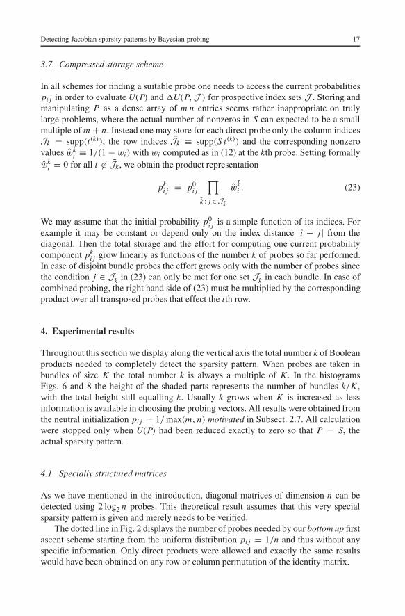
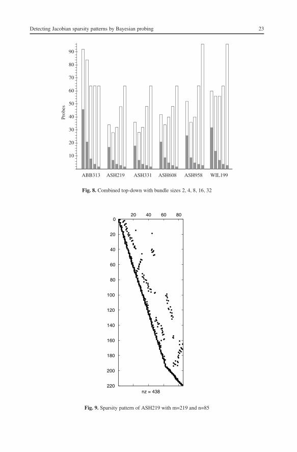
Fortunately, bundling by our top-down scheme does not increase the overall numberof probing vectors very much, as was already observed on the random matrices and cannow be seen in Fig. 8. The entries in Fig. 8 are slightly reminiscent of speed-up tables inparallel computing, where the wall-clock times scale almost inversely with the numberof processes. Here the number of bundle probes k/K represented by the shaded columnparts are almost reciprocal to the size K of each bundle. For the natural choice K = 32,we never need more than 3 bundle probes, of which the first one is computed almostcompletely blind, since all entries of the initial P are again chosen equal to the neutralvalue 1/ min(m, n).

As one can see in Fig. 9 the sparsity patterns of the Harwell-Boeing matrix ASH219has a certain degree of regularity, but it is by no means trivial. To be able to figure out thatpattern in just two bundle probes must be considered a very satisfactory achievement ofthe proposed approach.

5. Summary and discussion

In this paper we have developed a sequential probing scheme for determining thesparsity pattern of Jacobian matrices for vector functions defined by computer pro-


Fig. 8. Combined top-down with bundle sizes 2, 4, 8, 16, 32

20 40 60 800

20

40

60

80

100

120

140

160

180

200

220nz = 438

Fig. 9. Sparsity pattern of ASH219 with m=219 and n=85


grams. The problem specific input for this Bayesian estimation procedure consists ofBoolean Jacobian-vector products, which can be generated either by differencing orsuitably adapted automatic differentiation software. In the former case there is a re-mote possibility that false zeros are detected due to exact cancellations at the currentargument.

The dependence information generated by automatic or algorithmic differentiationis more reliable, and in its reverse mode one can also evaluate Boolean products ofthe transpose Jacobian at a similar cost. As demonstrated on the arrowhead example inFig. 3, this capability is very useful if the Jacobian in question happens to have some(nearly) dense rows. For this and other highly structured square matrices, we found thatthe total number of probing vectors required grew only logarithmically as a functionof the dimension n. The same observation applies to randomly generated matrices witha uniformly bounded number of nonzeros per row. Moreover, if test vectors were bundledin groups of up to 32 the total number of test vectors grew only by a factor less thantwo in all cases. Especially gratifying and still a little surprising is that the sparsitypatterns of several sizable matrices from the Boeing test collection could be identified injust two or three bundle probes, with the first one being selected without any structuralinformation.

There are several aspects that warrant further examination and improvement. First,it seems likely that the number of probes can be bounded on certain classes of matrices.Possibly a probabilistic analysis could also verify that the expected number of probeson randomly sparse matrices satisfies a relation similar to our conjecture (24). Thesequential updating approach may lead to some probabilities pi j ’s remaining below 1even though a simultaneous analysis of all probing results would reveals them alreadyas being 1. While this information may be a little hard to come by, it implies that allprobes involving column j or row i provide no information regarding other elementsin row i or column j , respectively. Therfore, an implementation of the simultaneousapproach with careful attention to the data structures used to store the probing resultsalready gathered may well be worthwhile.

Even when the updated probabilities can be (re)computed very efficiently, it wouldappear that at least our top-down procedure is much too costly. Some closer analysisof the similarity measure (22) and other optimization heuristics should lead to a fasterbundle calculation. Possibly, one might even be more general and allow overlappingindex sets Jk within each bundle probe.

Also, some more thought should be given to the initialization of the probabilitydistribution, which was simply uniform equal to 1/ min(n, m) in all our test calculations.In many applications it would make sense to initialize pi j as a function of some “distancemeasure” between the jth independent and the ith dependent variable. The closer theyare the more likely they are to interact, as is certainly the case in discretizations ofdifferential equations with possibly irregular grids. Then using the Euclidean distancebetween the associated grid points would seem rather natural.

Acknowledgements. The authors gratefully acknowledge the advice of Prof. D. Ferger and Dr. J. Franz of theInstitute of Stochastics in the Department of Mathematics at the Technical University of Dresden. They arealso thankful for the referee’s comments, which helped them to significantly improve the readability of thepaper.


References

[AZ85] Assaf, D., Zamir, S. (1985): Optimal Sequential Search: A Bayesian Approach. Ann. Statist. 13,1213–1221

[AC+92] Averick, B.M., Carter, R.G., Moré, J.J., Xue, G.-L. (1992): The MINPACK-2 test problem col-lection. Preprint MCS–P153–0692, ANL/MCS–TM–150, Rev. 1, Mathematics and ComputerScience Division, Argonne National Laboratory, Argonne, IL

[BB+96] Berz, M., Bischof, C.H., Corliss, G., Griewank, A., eds. (1996): Computational differentiation–techniques, applications, and tools. SIAM, Philadelphia

[BCK95] Bischof, C.H., Carle, A., Khademi, P.M. (1995): Fortran 77 Interface Specification to theSparsLinC 1.0 Library. ANL/MCS-TM-196, Mathematics and Computer Science Division, Ar-gonne National Laboratory, Argonne, IL

[BK+97] Bischof, C.H., Khademi, P.M., Bouaricha, A., Carle, A. (1997): Efficient computation of gradientsand Jacobians by dynamic exploitation of sparsity in automatic differentiation. Optim. MethodsSoftw. 7, 1–39

[BSG96] Bjørstad, P., Smith, B., Gropp, W. (1996): Domain decomposition: Parallel multilevel methodsfor elliptic partial differential equations. Cambridge University Press

[CF+01] Corliss, G., Faure, C., Griewank, A., Hascoët, L., Naumann, U., eds. (2001): Automatic Differen-tiation: From Simulation to Optimization. Springer

[CM84] Coleman, T.F., Moré, J.J. (1984): Estimation of sparse Jacobian matrices and graph coloringproblems. SIAM J. Numer. Anal. 20), 187–209

[CP+74] Curtis, A.R., Powell, M.J.D., Reid, J.K. (1974): On the estimation of sparse Jacobian matrices. J.Inst. Math. Appl. 13, 117–119

[CV95] Coleman, T.F., Verma, A. (1998): The efficient computation of sparse Jacobian matrices usingAutomatic Differentiation. SISC, 19(4), 1210–1233

[DGL] Duff, I.S., Grimes, R.G., Lewis, J.G.: Users’ Guide for the Harwell-Boeing Sparse Matrix Collec-tion (Release I). Research and Technology Division, Boeing Computer Services, Mail Stop 7L-2,P.O. Box 24236, Seatle, WA98124-0346, USA

[Fle00] Fleischer, L. (2000): Recent progress in Submodular Minimization. OPTIMA 64, Math. Prog.Soc. Newslett., Univ. Florida

[GK00] Giering, R., Kaminski, T.: Generating recomputations in reverse mode AD. In: Corliss et al.[CF+01], chap. 32

[GK01] Giering, R., Kaminski, T. (2001): Automatic Sparsity Detection. Draft, March 2001[GM01] Griewank, A., Mitev, C.: Verifying Jacobian Sparsity. In: Corliss et al. [CF+01], chap. 31[GR02] Griewank, A., Riehme, J.: Covering Zeros and Isolating Nonzeros in Sparse Jacobians. In prepar-

ation[Gri00] Griewank, A. (2000): Evaluating Derivatives, Principles and Techniques of Algorithmic Differ-

entiation. Number 19 in Frontiers in Appl. Math. SIAM, Philadelphia[GGU96] Geitner, U., Griewank, A., Utke, J.: Sparse Jacobians by Newsam/Ramsdell. In [BB+96], pp. 161–

172[GJ+96] Griewank, A., Juedes, D., Utke, J. (1996): ADOL–C, a package for the automatic differentiation of

algorithms written in C/C++. ACM Trans. Math. Software 22, 131–167, http://www.math.tu-dresden.de/wir/project/adolc/

[Hoc97] Hochbaum, D.S., ed. (1997): Approximation Algorithms for NP-Hard Problems. PWS PublishingCompany, 20 Park Plaza, Boston

[ST98] Shahadat Hossain, A.K.M., Steihaug, T. (1998): Computing a sparse Jacobian matrix by rows andcolumns. Optimization Methods and Software 10, 33–48

[NR83] Newsam, G.N., Ramsdell, J.D. (1983): Estimation of sparse Jacobian matrices. SIAM J. Alg. Disc.Meth. 4(3), 404–417

[KS79] Kimeldorf, G., Smith, F.H. (1979): Binomial Searching for a Random Number of MultinomiallyHidden Objects. Management Sci. 23, 1115–1126

[Lin95] Lindley, D.V. (1995): Bayesian Statistics, A Review. CBMS-NSF Regional Conference Series inAppl. Math. SIAM, University College London

Detecting Jacobian sparsity patterns by Bayesian probinglennart/drgrad/Griewank2002.pdf ·...

Documents

Transcript of Detecting Jacobian sparsity patterns by Bayesian probinglennart/drgrad/Griewank2002.pdf ·...