Detailed Methodology of Geospatial Fire Behavior Analyses

for the Savannah River Site

November 19, 2010

Prepared by LaWen Hollingsworth and Laurie Kurth

DE- AI09-00SR22188 TECHNICAL REPORT 2010 10-16-R

Three data sources were utilized to compare and contrast fire behavior modeling outputs (Table 1) from FlamMap for the Savannah River Site (SRS) in South Carolina.

Table 1. Data source for each FlamMap input theme

1Scott and Burgan’s (2005) 40 Fire Behavior Fuel Models (FBFM)

2Anderson’s (1983) 13 Fire Behavior Fuel Models (FBFM)

The merge function was used in ArcMap (Spatial Analyst > Raster Calculator) to modify fuel models as described above.

Merge function example in Raster Calculator: fbfm13_lkst = merge([lakes_98],[stream_98],[fbfm13_mod])

All fuel models were verified with local resource specialists for accuracy.

FlamMap Theme

Custom FCCS LANDFIRE Southern Wildfire Risk

ASPECT LANDFIRE Range = -1 – 359° -1 values (flat ground) retained

Range = 0 – 270°

SLOPE LANDFIRE Range = 0 – 28% Range = 0 – 54%

ELEVATION LANDFIRE Range = 19 – 150 m Range = 17 – 151 m

CANOPY BULK DENSITY

Local stand data, Range = 0 – 70, Units = kg/m

3 * 100

Range = 0 – 24, Units = kg/m

3 * 100

LANDFIRE and local stand data both used.

CANOPY BASE HEIGHT

Local stand data, Range = 0 – 177, Units = m * 10

Range = 0 – 100, Units = m * 10

LANDFIRE and local stand data both used.

CANOPY COVER

Local stand data, Range = 0 – 97%

Range = 0 – 95% Range = 0 – 65%

STAND HEIGHT

Local stand data, Range = 0 – 375 Units = m * 10

Range = 0 – 375, Units = m * 10

LANDFIRE and local stand data both used.

FUEL MODEL Custom fuel models developed from FCCS fuelbeds. Augmented SRS area with LANDFIRE data to fill in the landscape (used FBFM40

1). Have 95 records

= 0 in the SRS (there were some missing values in 2 stands). Refined with local data to better represent lakes and streams (FM 98) and 2-track roads (FM 101).

Used FBFM132 and

FBFM401. Both were refined

with local data to better represent lakes and streams (FM 98). The FBFM 13 were also updated to better represent unburnable fuel models (FM 91, 93, 99) and 2-track roads (FM 101).

FBFM132. The original fuel

model classification was modified to better represent unburnable fuel models (FM 91, 96, 97, 98, 99) and 2-track roads (FM 101) based on local data.

Number of FlamMap Runs

8 Runs (4 using FLI custom fuel model file, 4 using ROS custom fuel model file) Moderate Cond. – 10 mph, 30 mph Dry Cond. – 10 mph, 30 mph

8 Runs (4 for FBFM132 and 4 for FBFM401) Moderate Cond. – 10 mph, 30 mph Dry Cond. – 10 mph, 30 mph

8 Runs (4 for SWRA/LANDFIRE combo and 4 for SWRA/stand data combo) Moderate Cond. – 10 mph, 30 mph Dry Cond. – 10 mph, 30 mph

Eight input themes were used to construct each landscape file (LCP) to be used in FlamMap: canopy cover, canopy bulk density, canopy base height, stand height, fuel models, elevation, slope, and aspect. The LFDAT (LANDFIRE Data Access Tool v. 2.1) Raster Utilities function was used in ArcMap to build each LCP (Figure 1). Five LCP files were built: (1) FCCS (Fuel Characteristics Classification System) with canopy characteristics from local stand data and custom fuel models, (2) LANDFIRE data using FBFM13, (3) LANDFIRE data using FBFM40, (4) Southern Wildfire Risk Assessment data with LANDFIRE canopy data, and (5) Southern Wildfire Risk Assessment data with canopy characteristics from local stand data.

FlamMap requires canopy data to calculate wind reduction factors. A seen in Figure 1, the user can choose whether to include canopy characteristics when building a LCP. If a LCP is imported into FlamMap without canopy characteristics, these may be defined in FlamMap (refer to Figure 2, where the input selections are grayed out). This is not the preferred method, as there would be no variability between stands across the landscape. Southern Wildfire Risk Assessment data does not include canopy characteristics; this data was provided by LANDFIRE or local stand data.

Figure 1. Screen capture of the LFDAT Tool used to create a landscape file

Table 2. Moisture content for dead and live

fuels

Once the LCP files were ready, five FlamMap projects were built. Each FlamMap project uses one of the five LCP files and includes runs with differing fuel moisture files. The moderate situation uses high fuel moistures while the dry situation uses low fuel moistures. The Savannah River Remote Automated Weather Station (RAWS)

Moderate Dry 1-hr 7% 5%

10-hr 10% 7%

100-hr 15% 12%

Live Herbaceous 80% 60%

Live Woody 140% 110%

data was used as a reference to compile the fuel moisture files (Table 2). The moderate condition and dry condition were both run with 10-mph and 30-mph windspeeds to determine the effect of wind on fire behavior. The following screen captures show the inputs used for each FlamMap run for the LANDFIRE and Southern Wildfire Risk Assessment data (Figures 2, 3, and 4).

Figure 2. FlamMap Inputs screen

Figure 3. FlamMap Fire Behavior Outputs screen

Figure 4. FlamMap MTT Burn Probabilities screen

For FCCS, FlamMap requires an additional file (FMD file) as these are custom fuel models. The fireline intensity (FLI) FMD file is used in FlamMap for flame length and crown fire activity outputs (Figures 5 and 6). The rate of spread (ROS) FMD is used for rate of spread and burn probability outputs (Figures 7, 8, and 9).

Figure 5. FlamMap Inputs screen for FCCS (flame length and crown fire activity)

Figure 6. FlamMap Fire Behavior Outputs screen for FCCS (flame length and crown fire activity)

Figure 7. FlamMap Inputs screen for FCCS (rate of spread and burn probabilities)

Figure 8. FlamMap Fire Behavior Outputs screen for FCCS (rate of spread and burn probabilities)

Figure 9. FlamMap MTT Burn Probabilities screen for FCCS (rate of spread and burn probabilities)

Once a FlamMap simulation was complete, ASCII files were exported for flame length, rate of spread, crown fire activity, and burn probability. All the FlamMap outputs were exported as metric data. Each FlamMap project was saved using the File>Save and Archive command. At this point, the data can be taken sequentially through a number of steps in ArcCatalog or the AMLs can be used that were developed to process the data. The benefit to using an AML is that it is quicker, reduces the potential for human error, and is an effective way to work with grids. In ArcCatalog, the ASCII files are converted to rasters using the batch processor (Figure 10). The crown fire activity files were assigned to integer data and all other files were converted to floating data. All grids need to be assigned the same projection as the input rasters (NAD 1983 UTM Zone 17N) using the batch processor (Figure 11).

Figure 10. Batch conversion from ASCII to raster in ArcCatalog

Figure 11. Batch projection definition for rasters in ArcCatalog

The naming convention uses the following abbreviations/acronyms:

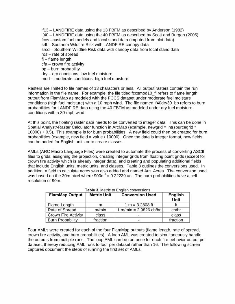
lf13 – LANDFIRE data using the 13 FBFM as described by Anderson (1982) lf40 – LANDFIRE data using the 40 FBFM as described by Scott and Burgan (2005) fccs –custom fuel models and local stand data (imputed from plot data) srlf – Southern Wildfire Risk with LANDFIRE canopy data srsd – Southern Wildfire Risk data with canopy data from local stand data ros – rate of spread fl – flame length cfa – crown fire activity bp – burn probability dry – dry conditions, low fuel moisture mod – moderate conditions, high fuel moisture Rasters are limited to file names of 13 characters or less. All output rasters contain the run information in the file name. For example, the file titled fccsmod10_fl refers to flame length output from FlamMap as modeled with the FCCS dataset under moderate fuel moisture conditions (high fuel moisture) with a 10-mph wind. The file named lf40dry30_bp refers to burn probabilities for LANDFIRE data using the 40 FBFM as modeled under dry fuel moisture conditions with a 30-mph wind. At this point, the floating raster data needs to be converted to integer data. This can be done in Spatial Analyst>Raster Calculator function in ArcMap (example, newgrid = int(sourcegrid * 10000) + 0.5). This example is for burn probabilities. A new field could then be created for burn probabilities (example, new field = value / 10000). Once the data is integer format, new fields can be added for English units or to create classes. AMLs (ARC Macro Language Files) were created to automate the process of converting ASCII files to grids, assigning the projection, creating integer grids from floating point grids (except for crown fire activity which is already integer data), and creating and populating additional fields that include English units, metric units, and classes. Table 3 outlines the conversions used. In addition, a field to calculate acres was also added and named Arc_Acres. The conversion used was based on the 30m pixel where 900m2 = 0.22239 ac. The burn probabilities have a cell resolution of 90m.

Table 3. Metric to English conversions

FlamMap Output Metric Unit Conversion Used English Unit

Flame Length m 1 m = 3.2808 ft ft

Rate of Spread m/min 1 m/min = 2.9826 ch/hr ch/hr

Crown Fire Activity class - class

Burn Probability fraction - fraction

Four AMLs were created for each of the four FlamMap outputs (flame length, rate of spread, crown fire activity, and burn probabilities). A loop AML was created to simultaneously handle the outputs from multiple runs. The loop AML can be run once for each fire behavior output per dataset, thereby reducing AML runs to four per dataset rather than 16. The following screen captures document the steps of running the first set of AMLs.

STEP 1. Open the Arc command line program

STEP 2. Create a workspace (“cw” command) and define the workspace (“w” command).

STEP 3. The loop AML must be opened using a text editor (such as notepad). The two

symbols, shown as /*, null that command line. Therefore, to run the loop AML for the four flame length outputs there will not be a /* in front of that line of text. It is important to have the AMLs and grids in the same folder initially; the data can be reorganized later.

STEP 4. Run the AML using the “&r” command.

This just shows the AML running…

STEP 5. Repeat Steps 3 – 4.

Showing Step 4 again.

AMLs were also created that clip the landscape down to the project area, in this case the SRS. A mask grid must be provided; this is simply the project area in raster format. A loop AML was also created. These AMLs work exactly the same as demonstrated above. There are a few hints to working in Arc. First, you must create a workspace. The workspace is simply the folder that contains the data in which you will be working with. Second, if you get an error message check to make sure spelling is correct. If ArcMap is also open, ensure that no value attribute tables are open while running the AMLs. The following lists a few of the commands that can be entered at the Arc prompt. cw – create workspace w – define workspace lg – list grids in that workspace &r – to run an AML tables – to work with a value attribute table (vat)

grid – to work with functions specific to rasters q – quit Arc ↑ - allows you to scroll up through previous commands on current command line

Statistics by Fuel Model In order to evaluate mean flame length and rate of spread by FBFM for LF40, LF13, SRLF, and SRSD data sources the following steps were completed. Statistics were not generated for the FCCS data as these are custom fire behavior fuel models. In addition, minimum and maximum values were also generated. The first step is to combine the four output grids for each data source for the fire parameter in question to the FBFM grid for that data source (Figure 12).

Figure 12. Combine function usage in Arc showing highlighted section combining the different burn

probabilities for the four fuel moisture and windspeed scenarios with the surface fire behavior fuel model

The next step is to join the data in the new grid back to the source grid to bring forth the necessary data fields, as the new grid contains all the VALUE fields from the source grids (Figures 13 and 14).

Figure 13. Value attribute table from the new grid before joins

Figure 14. An example of using the join command in ArcMap

Once the four join operations have been performed, a new grid can be exported that contains all the necessary fields from the source grids (Figure 15). All extra fields can now be deleted (Figure 16). As a side note, the fields in the rate of spread grids had the “chhr” fields renamed to “chh”. Two AMLs can be run at this point. The first AML is a loop AML that calls another AML up and cycles through all scenarios for that data source to create three zonal statistics for each scenario including zonal mean, zonal min, and zonal max. This first AML is, as an example, called SRSD_StatsLoop.aml. This AML is run twice, once for flame length and once for rate of spread, so each line must be nulled (/*) appropriately. All the zonalstats grids have units that have been multiplied by 1000 so they are integer rather than floating point data. The second AML combines all the single zonalstats grids into one grid along with the FBFM. This second AML is called CombineStats.aml and calls for the user to enter the project name (i.e. SRSD) and the fire parameter of interest (i.e. flame length or fl). This second AML must be run directly after the first to work correctly for each fire behavior parameter. This grid can then be exported

as a DBF file (Figure 17). The DBF file can be opened in Excel to create new fields that represent floating data and then create a pivot table.

Figure 15. Exporting a new grid once all joins are complete

Figure 16. Value attribute table from new exported grid created

from joined data once extra fields have been deleted

Figure 17. Exporting a grid as a DBF file

Once the DBF file has been imported to Excel, the value and count fields can be copied, and each of the zonalstats can be divided by 1000 to yield the actual non-integer value (Figure 18).

Figure 18. Creating the real values from the integer zonalstats values