M28876 Fiber Optic Connectors - Koehlke … Fiber Optic Connectors • 1. M28876 Fiber Optic Connectors

Design of High-Capacity Fiber-OpticTransport Systems
April 28, 2000 ZML: Ditech
Zhi M. Liao
The Institute of OpticsUniversity of Rochester
Advisor: Govind P. Agrawal
Design of High-Capacity Fiber-Optic Transport System
by
Zhi Ming Liao
Submitted in Partial Fulfillmentof the
Requirements for the DegreeDoctor of Philosophy
Supervised byProfessor Govind P. Agrawal
The Institute of OpticsThe College
School of Engineering and Applied Sciences
University of RochesterRochester, New York
2001

ii
dedicated toMom, Dad, ZJ, and Grandma

iii
Curriculum Vitae
The author was born in Canton, China. He immigrated with his family to Florida
when he was eleven. He learned English at Nova middle school and then graduated
as the valedictorian of Lake Worth high school class of 1991. He enrolled at the Uni-
versity of Rochester as a Bausch-Lomb scholar and graduated with a degree in optical
engineering and a minor in Electrical Engineering with High Distinction in 1995. He
received the School of Engineering and Applied Science’s Hook’s award for displaying
exemplifying interest in the engineering disciplines and for his active involvement in
the various student engineering societies including the IEEE (president), OSA (vice-
president), and Tau Beta Pi. Encouraged by the Optics faculty, he joined the Ph.D.
program at the University of Rochester in the fall of 1995. He was awarded a Mas-
ter of Science in Optics in 1996. During the course of his education at Rochester,
he also spent summers working in Lawrence Livermore National Laboratory (1994 –
1996) and Los Alamos National Laboratory (1999) performing research ranging from
implementing optical testing techniques to modeling soliton dynamics.

CURRICULUM VITAE iv
Publications
• Z. M. Liao and G. P. Agrawal, “Role of Distributed Amplification in DesigningHigh Capacity Soliton Systems,”IEEE Photonics Technology Letters, Submittedfor Review (2000).
• Z. M. Liao and G. P. Agrawal, “Mode-Partition Noise in Fiber Lasers,”Electron-ics Letters, 36, 1188-1189 (2000).
• Z. M. Liao, C. J. McKinstrie, and G. P. Agrawal, “Importance of Prechirpingin Constant-Dispersion Fiber Links with a Large Amplifier Spacing,”Journal ofOptical Society of America B, 17, 514-518 (2000).
• Z. M. Liao and G. P. Agrawal, “High-Bit-Rate Soliton Transmission Using Dis-tributed Amplification and Dispersion Management,”;IEEE Photonics Technol-ogy Letters, 11, 818-820 (1999).
• J. Inman, S. Houde-Walter, B. McIntyre, Z. M. Liao, R. Parker, and V. Sim-mons, “Chemical Structure and the Mixed Mobile Ion Effect in Ag-for-Na IonExchange in Aluminosilicate Glasses,”Journal of Noncrystalline Solids, 191,85-92 (1996).
• Z. M. Liao, S. J. Cohen and J. R. Taylor, “Total Internal Reflection Microscopy(TIRM) as a Nondestructive Subsurface Assessment Tool,”Proceedings of An-nual Symposium on Optical Materials for High Power Lasers, Boulder, CO. Oc-tober 1994.
CURRICULUM VITAE v
Presentations
• G. P. Agrawal and Z. M. Liao,“Mode-partition noise in fibre lasers,” OSA AnnualMeeting, Rhode Island, October 2000.
• Z. M. Liao and G. P. Agrawal,“Distributed Amplification,” Invited talk, Corning,NY, June 2000.
• Z. M. Liao,“Implementation of Distributed Amplification for High Speed SolitonTransmission,” Institute of Optics Industrial Associate’s Meeting, Rochester, NY,October 1999.
• Z. M. Liao, C. J. McKinstrie, G. P. Agrawal ”A Novel Operating Regime forPeriodically Amplified Fiber Links: Role of Prechirping,” OSA Annual Meeting,Santa Clara, CA, October 1999.
• Z. M. Liao and I. Gabitov, “Slow Dynamics of Optical Pulse in Optical Fibers,”Summer seminar series, Los Alamos, NM, August 1999.
• Z. M. Liao and G. P. Agrawal, “Design of Soliton Communication Systems us-ing Distributed Amplification,” OSA Annual Meeting, Baltimore, MD, October1998.

vi
Acknowledgments
It may be challenging to fill 100 pages of technical material for this thesis, but it
certainly would be a breeze to fill 100 pages to acknowledge all of the people who
made this possible. Actually, the difficulty has been to reduce the list to a reasonable
size, so I would like to apologize in advance to anyone I may have forgotten due to my
deteriorating mental prowess. This is the price one must pay for a higher education. :-)
Mind: Since this is a scientific thesis, I would like to first thank those who have la-
bored to educate me. I would like to acknowledge Dr. Taras I. Lakoba for his guidance
in the realm of mathematics, Dr. Drew N. Maywar for being the best possible office-
mate, and Dr. Rene Essiambre for introducing me to numerical simulations. For taking
time off their busy lives to help proof read my thesis, I would like to thank the following
individuals: Stephanie Chen, Falgun Patel, Drew Maywar, Gina Jones, Shafique Jamal
and Kunal Kishore. I would also like to thank Professor Colin J. McKinstrie for his
help with varational analysis. Last and certainly not the least, I am gratefully indebted
to Professor Govind P. Agrawal, for his inhuman patience, boundless knowledge, and
above all, kind guidance.
ACKNOWLEDGEMENTS vii
Body&Spirit: I would like to thank Joan Christian, Gayle Thompson, and all the
staff at the Institute of Optics for making the place more like a home than a work place.
I like to thank my mentors: Simon Cohen for taking me under his wings at LLNL,
Dr. Ildar Gabitov for his guidance at LANL, and Dr. Falgun Patel for instructing me
the important technique of double-shaded boxes.
First of all, I would like to state that a moron does a body good. Without the
morons, graduate school would not have been so enjoyable. I like to thank the Bean,
Bhanu, Dave, KB, Gaby, Paul, Pete, Stephyjo and Steve for making Rochester a fun
place to live !
For Stephanie Chen, whose advice, friendship, and yes, being a bully were, I am
going have to create a new word here, ”inrepayable”, in the completion of this degree.
I can’t ever repay you, Steph, and I won’t, so don’t ask. :-)
My best bud, Anando Anwar Chowdhury, for always being there; for laughter, for
understanding, for making me part of his family, and for being half of “zandy”, a true
kindred spirit.
Lastly, Christine Thao La for her dedication in making my graduate life as chal-
lenging as possible. She compensates that by breathing love into my life.
Soul: Mom, Dad, Jing and Grandma, the foundation in which everything in my life
is based on.

viii
Abstract
We study the design of fiber-optic transport systems and the behavior of fiber am-
plifiers/lasers with the aim of achieving higher capacities with larger amplifier spacing.
Solitons are natural candidates for transmitting short pulses for high-capacity fiber-
optic networks because of its innate ability to use two of fiber’s main defects, fiber
dispersion and fiber nonlinearity to balance each other. In order for solitons to retain its
dynamic nature, amplifiers must be placed periodically to restore powers to compensate
for fiber loss. Variational analysis is used to study the long-term stability of a periodical-
amplifier system. A new regime of operation is identified which allows the use of a
much longer amplifier spacing.
If optical fibers are the blood vessels of an optical communication system, then
the optical amplifier based on erbium-doped fiber is the heart. Optical communication
systems can avoid the use of costly electrical regenerators to maintain system perfor-
mance by being able to optically amplify the weakened signals. The length of amplifier
spacing is largely determined by the gain excursion experienced by the solitons. We
propose, model, and demonstrate a distributed erbium-doped fiber amplifier which can

ABSTRACT ix
drastically reduce the amount of gain excursion experienced by the solitons, therefore
allowing a much longer amplifier spacing and superior stability.
Dispersion management techniques have become extremely valuable tools in the
design of fiber-optic communication systems. We have studied in depth the advan-
tage of different amplification schemes (lumped and distributed) for various dispersion
compensation techniques. We measure the system performance through the Q factor to
evaluate the added advantage of effective noise figure and smaller gain excursion.
An erbium-doped fiber laser has been constructed and characterized in an effort
to develop a test bed to study transmission systems. The presence of mode-partition
noise in an erbium-doped fiber laser was experimentally demonstrated. A numerical
model has been developed using the Langevin rate equations and its predictions are in
qualitative agreement with experimental data.

x
Table of Contents
1 Introduction 1
1.1 Motivation . . . . . . . . . . . . . . . . . . . . . . . . . . . . . . . . . 1
1.2 Historical Overview . . . . . . . . . . . . . . . . . . . . . . . . . . . . 3
1.2.1 Fiber-Optic Communication Systems . . . . . . . . . . . . . . 3
1.2.2 Optical Solitons . . . . . . . . . . . . . . . . . . . . . . . . . . 5
1.3 Thesis Overview . . . . . . . . . . . . . . . . . . . . . . . . . . . . . 7
1.3.1 Principle of Fiber-Optic Communication Systems . . . . . . . . 7
1.3.2 Outline . . . . . . . . . . . . . . . . . . . . . . . . . . . . . . 9
2 Theoretical Foundation 11
2.1 Introduction . . . . . . . . . . . . . . . . . . . . . . . . . . . . . . . . 11
2.2 Wave Propagation Equation . . . . . . . . . . . . . . . . . . . . . . . . 11
2.2.1 Dispersion . . . . . . . . . . . . . . . . . . . . . . . . . . . . 19
2.2.2 Fiber Loss . . . . . . . . . . . . . . . . . . . . . . . . . . . . 21
2.2.3 Nonlinear Schrodinger Equation . . . . . . . . . . . . . . . . . 22

CONTENTS xi
2.3 Optical Solitons . . . . . . . . . . . . . . . . . . . . . . . . . . . . . . 24
2.4 Split-Step Fourier Transform Method . . . . . . . . . . . . . . . . . . 26
2.5 Variational Technique . . . . . . . . . . . . . . . . . . . . . . . . . . . 29
2.6 Summary . . . . . . . . . . . . . . . . . . . . . . . . . . . . . . . . . 32
3 Chirped Solitons in Constant-Dispersion Fiber Links 33
3.1 Introduction . . . . . . . . . . . . . . . . . . . . . . . . . . . . . . . . 33
3.2 Guiding-Center Solitons . . . . . . . . . . . . . . . . . . . . . . . . . 34
3.3 Pre-Chirped Solitons . . . . . . . . . . . . . . . . . . . . . . . . . . . 37
3.3.1 Variational Results . . . . . . . . . . . . . . . . . . . . . . . . 38
3.3.2 Analytical Results . . . . . . . . . . . . . . . . . . . . . . . . 40
3.4 Numerical Results . . . . . . . . . . . . . . . . . . . . . . . . . . . . . 41
3.5 Summary . . . . . . . . . . . . . . . . . . . . . . . . . . . . . . . . . 47
4 Distributed Amplification in Constant-Dispersion Systems 49
4.1 Introduction . . . . . . . . . . . . . . . . . . . . . . . . . . . . . . . . 49
4.2 Erbium-Doped Fiber Amplifiers . . . . . . . . . . . . . . . . . . . . . 50
4.3 Distributed Erbium-Doped Fiber Amplifiers . . . . . . . . . . . . . . . 53
4.3.1 Modeling Gain in Distributed Fiber Amplifiers . . . . . . . . . 53
4.3.2 Small-Signal Solution . . . . . . . . . . . . . . . . . . . . . . 54
4.3.3 Numerical Solution . . . . . . . . . . . . . . . . . . . . . . . . 56
4.4 Raman Amplifier . . . . . . . . . . . . . . . . . . . . . . . . . . . . . 58

CONTENTS xii
4.4.1 Small Signal Analysis . . . . . . . . . . . . . . . . . . . . . . 60
4.4.2 Numerical Results . . . . . . . . . . . . . . . . . . . . . . . . 60
4.5 Amplifier Performance . . . . . . . . . . . . . . . . . . . . . . . . . . 62
4.6 Summary . . . . . . . . . . . . . . . . . . . . . . . . . . . . . . . . . 65
5 Dispersion-Management Systems 67
5.1 Introduction . . . . . . . . . . . . . . . . . . . . . . . . . . . . . . . . 67
5.2 Dispersion Managed Soliton . . . . . . . . . . . . . . . . . . . . . . . 69
5.2.1 Variational Analysis . . . . . . . . . . . . . . . . . . . . . . . 69
5.2.2 Two-Step Dispersion Map . . . . . . . . . . . . . . . . . . . . 70
5.2.3 Dense Dispersion Management . . . . . . . . . . . . . . . . . 73
5.3 System Performance . . . . . . . . . . . . . . . . . . . . . . . . . . . 75
5.3.1 Amplifier Noise . . . . . . . . . . . . . . . . . . . . . . . . . . 75
5.3.2 Numerical Results . . . . . . . . . . . . . . . . . . . . . . . . 76
5.4 Summary . . . . . . . . . . . . . . . . . . . . . . . . . . . . . . . . . 81
6 Fiber Lasers 83
6.1 Introduction . . . . . . . . . . . . . . . . . . . . . . . . . . . . . . . . 83
6.2 Experimental Setup . . . . . . . . . . . . . . . . . . . . . . . . . . . . 83
6.2.1 Output Power . . . . . . . . . . . . . . . . . . . . . . . . . . . 84
6.2.2 Frequency Characteristics . . . . . . . . . . . . . . . . . . . . 85
6.3 Mode-Partition Noise . . . . . . . . . . . . . . . . . . . . . . . . . . . 86

CONTENTS xiii
6.3.1 Experimental Observation . . . . . . . . . . . . . . . . . . . . 87
6.3.2 Mode-Partition Noise Theory . . . . . . . . . . . . . . . . . . 88
6.4 Summary . . . . . . . . . . . . . . . . . . . . . . . . . . . . . . . . . 91
7 Conclusions 93
7.1 Overview . . . . . . . . . . . . . . . . . . . . . . . . . . . . . . . . . 93
7.2 Constant-Dispersion Fibers . . . . . . . . . . . . . . . . . . . . . . . . 93
7.3 Dispersion-Management Technique . . . . . . . . . . . . . . . . . . . 96
7.4 Fiber-Laser Dynamics . . . . . . . . . . . . . . . . . . . . . . . . . . 97
7.5 Summary . . . . . . . . . . . . . . . . . . . . . . . . . . . . . . . . . 97
Bibliography 99
A Calculating Pulse Parameters 105
A.1 Gaussian Pulse . . . . . . . . . . . . . . . . . . . . . . . . . . . . . . 105
A.2 Hyperbolic Secant Pulse . . . . . . . . . . . . . . . . . . . . . . . . . 107
B Bit-Error Rate 109

xiv
List of Tables
2.1 Parameters used in simulation of pulse broadening . . . . . . . . . . . 20
2.2 Parameters used in simulation of pulse spectrum broadening . . . . . . 24
2.3 Parameters used in simulation of soliton propagation . . . . . . . . . . 26
3.1 Parameters used in simulation of soliton propagation . . . . . . . . . . 37
6.1 Parameters used in simulation of fiber laser dynamics . . . . . . . . . . 90

xv
List of Figures
1.1 Capacity growth of fiber-optic communication systems. . . . . . . . . . 5
1.2 Basic elements of a fiber-optic communication system . . . . . . . . . . 7
1.3 Optical bit stream using NRZ and RZ formats . . . . . . . . . . . . . . 8
2.1 Pulse spreading due to GVD . . . . . . . . . . . . . . . . . . . . . . . 21
2.2 Pulse spreading due to GVD in the presence of fiber loss . . . . . . . . 22
2.3 Spectral broadening of optical pulse due to SPM . . . . . . . . . . . . . 25
2.4 Soliton pulse propagation . . . . . . . . . . . . . . . . . . . . . . . . . 27
2.5 Split-step Fourier transform method . . . . . . . . . . . . . . . . . . . 28
3.1 Amplitude variations of lumped amplification withLA=20 km and 0.2
dB/km loss. . . . . . . . . . . . . . . . . . . . . . . . . . . . . . . . . 36
3.2 Evolution of guiding-center soliton . . . . . . . . . . . . . . . . . . . . 38
3.3 Periodicity of soliton pulse through each amplifier unit . . . . . . . . . 39
3.4 Power and chirp requirements for propagation . . . . . . . . . . . . . . 42
3.5 Pulse evolution over single amplifier period . . . . . . . . . . . . . . . 44

LIST OF FIGURES xvi
3.6 Pulse evolution over single amplifier period . . . . . . . . . . . . . . . 45
3.7 Pulse evolution over multiple amplifier periods . . . . . . . . . . . . . 46
3.8 Pulse evolution over multiple amplifier periods . . . . . . . . . . . . . 47
3.9 Poincare map of pulse stability . . . . . . . . . . . . . . . . . . . . . . 48
4.1 Three level model of erbium-doped gain medium . . . . . . . . . . . . 50
4.2 Distributed-erbium doped amplifier link . . . . . . . . . . . . . . . . . 53
4.3 Bi-directional pumping of d-EDFA . . . . . . . . . . . . . . . . . . . . 54
4.4 Analytical and numerical solution of the forward, backward, and total
pump powers . . . . . . . . . . . . . . . . . . . . . . . . . . . . . . . 57
4.5 Pump power needed for various dopant levels . . . . . . . . . . . . . . 58
4.6 Maximum net gain for various dopant levels . . . . . . . . . . . . . . . 59
4.7 Pump power and gain variations of Raman amplifier . . . . . . . . . . . 61
4.8 Pulse evolution in lumped and distributed amplification . . . . . . . . . 63
4.9 Logarithmic plot of the pulse using distributed amplification . . . . . . 64
4.10 Pump power and gain variations of d-EDFA . . . . . . . . . . . . . . . 65
5.1 Two-step dispersion map . . . . . . . . . . . . . . . . . . . . . . . . . 70
5.2 Dense dispersion map . . . . . . . . . . . . . . . . . . . . . . . . . . . 74
5.3 Eye diagram of a 20-Gb/s system . . . . . . . . . . . . . . . . . . . . . 77
5.4 System performance of a 40-Gb/s DM soliton system using different
amplification schemes. . . . . . . . . . . . . . . . . . . . . . . . . . . 79
5.5 Spatial gain distribution of different amplification schemes . . . . . . . 80

LIST OF FIGURES xvii
5.6 System performance of a 80-Gb/s DM soliton system using different
amplification schemes. . . . . . . . . . . . . . . . . . . . . . . . . . . 81
5.7 Pulse interaction for 80-Gb/s soliton system . . . . . . . . . . . . . . . 82
6.1 Experimental configuration of the fiber laser . . . . . . . . . . . . . . . 84
6.2 Output power vs. pump current for the fiber laser . . . . . . . . . . . . 85
6.3 Output power vs. pump power for the fiber laser . . . . . . . . . . . . . 86
6.4 Spectrum of the pump output . . . . . . . . . . . . . . . . . . . . . . . 87
6.5 Spectrum of the fiber laser output . . . . . . . . . . . . . . . . . . . . . 88
6.6 Experimental observation of mode-partition noise . . . . . . . . . . . . 89
6.7 Simulation result of mode-partition noise . . . . . . . . . . . . . . . . 91

1
Chapter 1
Introduction
1.1 Motivation
The era of the information revolution is upon us. The internet has brought the world
closer together. Although voice traffic continues to grow at merely 3 to 5% per year,
the increase in data traffic will continue to expand global networks at an estimated rate
of 10 to 25 times over the next few years [1]. This demand for high-bit-rate commu-
nication systems has heralded fiber-optical lightwave systems as the savior, primarily
because of the extremely broad bandwidth associated with an optical carrier. This is
because the frequency of an optical carrier (∼ 100 THz) is five orders of magnitude
greater than the frequency of a microwave carrier (∼ 1 GHz) [2] and since the modula-
tion bandwidth is usually limited to a small fraction of the carrier frequency in digital
systems, this translates to roughly 100,000 times more capacity for a fiber optic com-
munication system. Despite this tremendous increase in system capacity, it barely able
to keep up with today’s demand.
Optical fibers are considered by many as God-sent for optical communications be-
cause of their many wonderful features: wave-guiding, low loss, and small nonlinear-
ity. However, as a system grows in capacity, its complexity also grows. Even though a

1.1. MOTIVATION 2
modern optical fiber suffers only a fraction of decibals (dB) per kilometer (km) of loss,
system lengths of hundreds and thousands of kilometers will accumulate enough losses
to demand the need of amplifiers. The introduction of erbium-doped fiber amplifiers
(EDFAs) [3] in the early 1990s made it possible to support systems with capacity of
tens and hundreds of gigabits per second (Gb/s) with an amplifier spacing of 50-100
km. Amplifiers need to be placed more frequently as system capacity increases when
solitons are used since the dispersion length scales quadratically with soliton width.
Thus, the demand on increasing capacity is causing the amplifier spacing to become
shorter, which can drive the cost so high that the solution will become impractical. The
placement of amplifier modules is therefore crucial in the design of high-capacity fiber
optic systems.
Furthermore, the performance of these high-capacity systems are often limited by
the lumped nature of the amplifiers. An alternative approach using distributed amplifi-
cation has become an exciting new avenue to explore. Distributed amplification using
stimulated Raman scattering (SRS) has already helped to produce terabits per second
system capacity (Tb/s) as well as longer transmissions distances without regeneration
[4–7]. In addition, the recent development of high power fiber/semiconductor pump
lasers will make distributed amplification an even more attractive option for future sys-
tems. The synthesis of distributed amplification into existing system architecture with
current technologies such as dispersion management and wavelength-division multi-
plexing (WDM) will bring forth the next generation of ultra-high-capacity fiber optic
communication systems.
This thesis explores the placement and design of optical amplifiers in constant-
dispersion systems as well as in dispersion management systems, and seeks to optimize

1.2. HISTORICAL OVERVIEW 3
the existing technology and to advance future technologies in the design of ultra-high-
capacity fiber-optic systems. A history of the evolution of optical communication is
presented next.
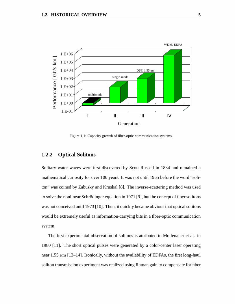
1.2 Historical Overview
Solitons have a rich history that dates all the way back to the early 1800s even though
fiber-optic communication systems have been in existence for less than 25 years. These
temporally separated entities are on course to collide and create the next generation of
ultra-high-capacity communication systems.
1.2.1 Fiber-Optic Communication Systems
The development of lasers in the 1960s and low loss fibers in the early 1970s made
possible the first fiber-optic communication system in 1978. These systems were able to
transmit signals at 100 Mb/s using multimode fibers operating near 0.85µm. Although
the repeater spacing was less than 10 km, it was sufficiently large than the repeater
spacing of the heritage coaxial system. This feature made fiber optic communication
system an attractive alternative for the future — thus the first generation of fiber-optic
systems was born [2].
The desire to reduce the number of regeneration units by increasing the repeater
spacing of the first generation systems quickly lead to the second generation system in
the early 1980s. The second generation system allowed for increased repeater spacing
by operating the system at the lower loss regime near 1.3µm. Additional improvements
were also made in optical fiber technology by the introduction of the single-mode fiber;

1.2. HISTORICAL OVERVIEW 4
this soon propelled the system capacity to Gb/s with repeater spacings in excess of 50
km. The system operation wavelength was further moved to 1.55µm to take advantage
of the lowest fiber loss for the third generation system introduced in the late 1980s.
The increased propagation distance allowed by lower fiber loss and the larger fiber
dispersion at 1.55µm introduced fiber dispersion as the next obstacle to tackle. The
dispersion problem was eventually solved by using dispersion-shifted fibers and single
longitudinal mode lasers to reduce the spreading of the transmitted pulse. Such systems
can operate in excess of 10 Gb/s with repeater spacings as large as 100 km [2].
The early generations of fiber-optic systems relied on repeaters to compensate fiber
loss through electrical amplification. These regeneration stations consisted of decoders
to transform the information from an optical domain to an electrical domain, electronic
amplifiers to reboost the signal, and transmitters to re-transform the information from
the electrical domain back to the optical signal. This process was an expensive ne-
cessity. The development of EDFAs during the 1990s provided a breakthrough which
allowed pulses to be optically amplified thus reducing the need of so many regener-
ation stations. This dramatically reduced the cost while provided a very dynamic and
transparent solution. Optical amplifiers have paved the way to another ground-breaking
technology — WDM. The WDM technique offered the ability to scale the system ca-
pacity via the same fiber by simply adding data channels using slightly different wave-
lengths [2]. The fourth generation systems boasted capacity of upwards of terabits per
second (Tb/s) — yet, the demand is still increasing.
1.2. HISTORICAL OVERVIEW 5
Feb. 13, 1998 ZML: Thesis Proposal
I II III IV1.E-01
1.E+00
1.E+01
1.E+02
1.E+03
1.E+04
1.E+05
1.E+06P
erfo
rman
ce [
Gb/
s-km
]
I II III IV
Generation
1. Progression of Lightwave Communication Systems
multimode
single-mode
DSF, 1.55 um
WDM, EDFA
Figure 1.1: Capacity growth of fiber-optic communication systems.
1.2.2 Optical Solitons
Solitary water waves were first discovered by Scott Russell in 1834 and remained a
mathematical curiosity for over 100 years. It was not until 1965 before the word “soli-
ton” was coined by Zabusky and Kruskal [8]. The inverse-scattering method was used
to solve the nonlinear Schrodinger equation in 1971 [9], but the concept of fiber solitons
was not conceived until 1973 [10]. Then, it quickly became obvious that optical solitons
would be extremely useful as information-carrying bits in a fiber-optic communication
system.
The first experimental observation of solitons is attributed to Mollenauer et al. in
1980 [11]. The short optical pulses were generated by a color-center laser operating
near 1.55µm [12–14]. Ironically, without the availability of EDFAs, the first long-haul
soliton transmission experiment was realized using Raman gain to compensate for fiber

1.2. HISTORICAL OVERVIEW 6
losses [15]. Since then, tremendous strides have been made in soliton-communication
systems by incorporating innovative technologies such as EDFAs, dispersion manage-
ment, WDM, in-line filters, etc. [2]. Field trials of soliton communication systems first
appeared in 1998 by Pirelli [16] and now, companies such as Algety Telecom has been
formed explicitly to exploit soliton’s advantages [1].
The semiconductor industry follows Moore’s law to describe the rate of the growth
of the processor speed. Moore’s law states that in general, the speed of the process-
ing chips doubles its system capacity every eight months. The capacity of public net-
work traffic has been however, exceeding this rate and doubling about every six months
[17]. While fiber loss has been addressed by the development of optical amplifiers (e.g.
EDFA, Raman), the problem with fiber dispersion and fiber nonlinearity still remained.
The next generation of fiber-optic communication system is focused on solving these is-
sues. We believe that optical solitons are the ultimate solution, since they can effectively
use the fiber nonlinearity to balance the accumulated dispersion. In order to maintain
the soliton stability over large amplifier spacings and long distances, distributed ampli-
fication must be incorporated to minimize system perturbations. The purpose of this
thesis is to contribute to the development of the next generation of high-capacity fiber-
optic communication systems by studying how to design soliton systems with different
dispersion management and amplification techniques.
1.3. THESIS OVERVIEW 7
1.3 Thesis Overview
1.3.1 Principle of Fiber-Optic Communication Systems
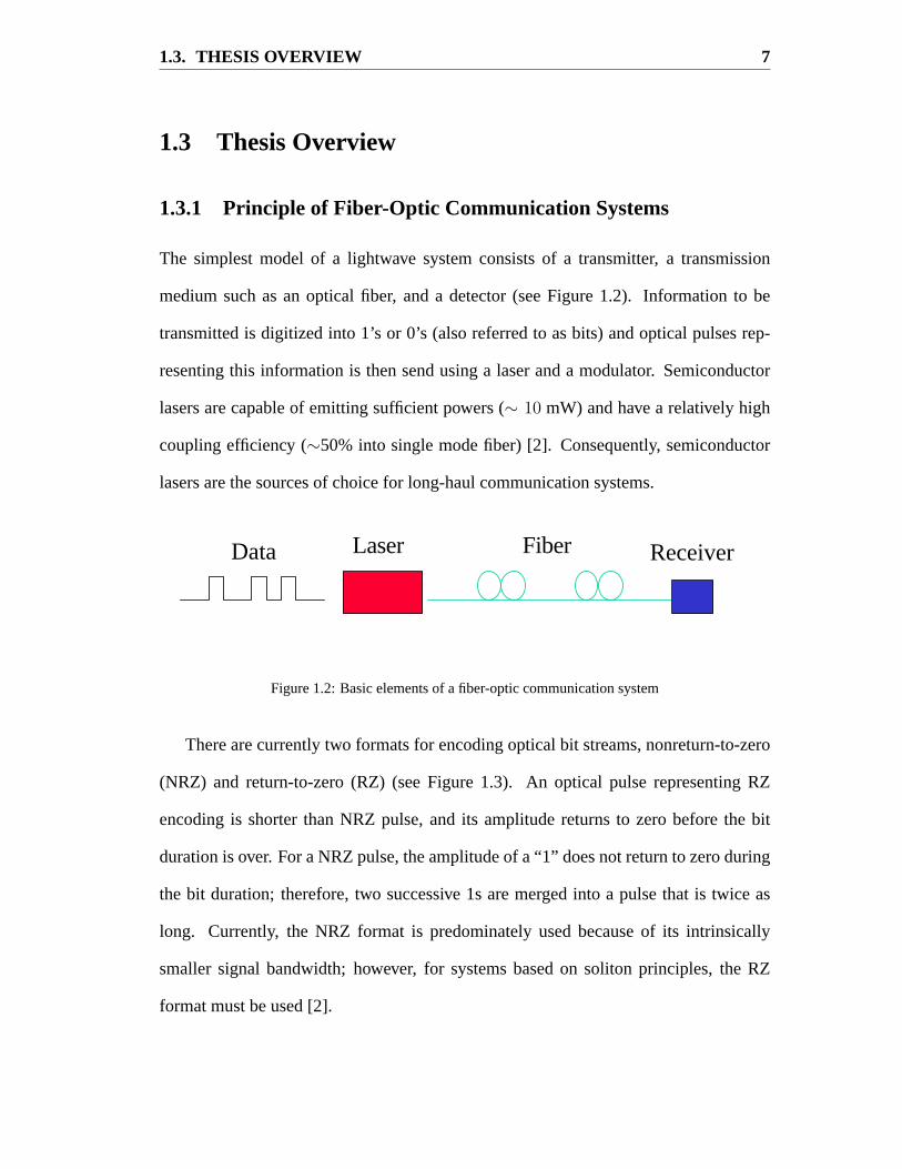
The simplest model of a lightwave system consists of a transmitter, a transmission
medium such as an optical fiber, and a detector (see Figure 1.2). Information to be
transmitted is digitized into 1’s or 0’s (also referred to as bits) and optical pulses rep-
resenting this information is then send using a laser and a modulator. Semiconductor
lasers are capable of emitting sufficient powers (∼ 10 mW) and have a relatively high
coupling efficiency (∼50% into single mode fiber) [2]. Consequently, semiconductor
lasers are the sources of choice for long-haul communication systems.
Feb. 13, 1998 ZML: Thesis Proposal
2.1 Single Channel Lightwave Communication Systems
• Transmitter - Laser Rate Equations• Fiber-Optic Communication Channel - NSE• Receiver - Responsitivity, Bit Error Rate (BER)
Data Laser Fiber Receiver
Figure 1.2: Basic elements of a fiber-optic communication system
There are currently two formats for encoding optical bit streams, nonreturn-to-zero
(NRZ) and return-to-zero (RZ) (see Figure 1.3). An optical pulse representing RZ
encoding is shorter than NRZ pulse, and its amplitude returns to zero before the bit
duration is over. For a NRZ pulse, the amplitude of a “1” does not return to zero during
the bit duration; therefore, two successive 1s are merged into a pulse that is twice as
long. Currently, the NRZ format is predominately used because of its intrinsically
smaller signal bandwidth; however, for systems based on soliton principles, the RZ
format must be used [2].

1.3. THESIS OVERVIEW 8
0 1 0 01 1 0
Data
NRZ
RZ
Figure 1.3: Optical bit stream using NRZ and RZ formats
The optical bit stream is transported through optical fibers from one location to an-
other. The capacity of a fiber-optic communication system is designated by the number
of bits it can send per second, or alternatively, by the inverse of the bit slot. Thus,
a system transmitting 100-ps pulses using NRZ or 25-ps pulses using RZ (with pulse
separation equal to four times the pulse width) will carry a single channel capacity of
10 Gb/s.
The receiver’s role is to convert the optical signal received from the optical fiber
back to the original electrical signal. Modern systems use the direct-detection scheme,
which typically consists of a semiconductor detector, a clock-recovery circuit, and
a decision-making circuit to identify bits as 1 or 0. The performance of fiber-optic

1.3. THESIS OVERVIEW 9
communication systems is characterized by the number of errors made per second as
counted by its receiver circuit, or the bit-error rate (BER). Typically, a system is spec-
ified as having error-free transmission when it has BER of less than10−9 [2]. With
novel coding algorithms, systems can gain several dB in performance using forward
error correction (FEC).
1.3.2 Outline
Chapter 2 provides the foundation of the theoretical and numerical analysis. We derive
the nonlinear Schrodinger equation from Maxwell’s equations and introduce the basic
fiber properties and how they affect the pulse propagation. We will also present numer-
ical and approximate analytical (variational analysis) techniques to solve the nonlinear
Schrodinger equation . These will provide tools to simulate systems as well as to opti-
mize parameters in system design.
Chapter 3 begins our investigation of designing soliton communication systems by
examining the periodicity of constant-dispersion systems through variational analysis.
We introduce the concept of a guiding-center soliton (GCS) and the limitations it im-
poses on the amplifier spacing of the system. We are then able to exploit the analytical
results to use the chirp of soliton pulses to extend the amplifier spacing beyond the
guiding-center soliton regime. We show through numerical simulations the effective-
ness of the variational results and validate the technique as a valuable tool in exploring
and optimizing the complex parameter space of a soliton communication systems.
Chapter 4 provides the foundation of implementing distributed amplification in
fiber-optic communication systems. We first introduce the governing equations for
distributed-EDFA as well as Raman amplification, and then provide some approxi-

1.3. THESIS OVERVIEW 10
mated analytical solutions to illustrate some basic principles such as pump depletion
and gain saturation. These equations are solved numerically and the solution is then
incorporated into the nonlinear Schrodinger equation to evaluate the effectiveness of
distributed amplification.
Chapter 5 introduces the technique of dispersion management for combating the
fiber dispersion problem. A two-step dispersion map as well as the novel dense dis-
persion map are introduced along with variational-analysis results in calculating the
optimal launching condition for a given map. We also show how variational analysis
has been applied to the study of dispersion management systems. We show how the sys-
tem performance is characterized with the inclusion of noise, and assimilate different
amplification schemes with dispersion-management techniques to investigate various
design rules.
Chapter 6 characterizes the operation of a fiber laser. Specifically, it focuses on the
mechanism of mode-partition noise in a fiber laser. We present the experimental setup
and discuss the system operation of the fiber laser. We also present our theoretical
formulation and examine the numerical results and compare them to experimental data.
Chapter 7 summaries the main results and findings of the thesis and provides in-
sights for future investigations.

11
Chapter 2
Theoretical Foundation
2.1 Introduction
The design of a fiber-optic communication system requires an understanding of the
nonlinear propagation of optical pulses, with emphasis on fiber losses and fiber dis-
persion. In this chapter, we present equations that govern this process; namely, the
nonlinear Schrodinger equation supporting picosecond pulses and higher order effects
such as stimulated Raman scattering (SRS). Since the nonlinear Schrodinger equation
cannot be solved in a closed form, numerical techniques such as the split-step Fourier
transform method will be presented to help study it. Variational analysis will also be
presented as a valuable analytical tool to give qualitative understanding of this complex
process.
2.2 Wave Propagation Equation
As always, we begin our analysis of the optical signal propagation through an optical
fiber with Maxwell’s equations. Furthermore, we can safely assume that the optical
fiber is a non-magnetic medium without any free surface charges. Maxwell’s equations

2.2. WAVE PROPAGATION EQUATION 12
are then given as (in SI units) [9]
~5× ~E = −∂ ~B∂t
, (2.1)
~5× ~H =∂ ~D
∂t, (2.2)
~5 · ~D = 0, (2.3)
~5 · ~B = 0, (2.4)
where~E is the electric field,~H is the magnetic field,~D is the electric flux density, and
~B is the magnetic flux density. The flux densities within an optical fiber can be written
as
~D = εo~E + ~P , (2.5)
~B = µo~H, (2.6)
whereεo andµo are the vacuum permittivity and permeability respectively, and~P is the
induced electric polarization.
The wave equation can be derived by first taking the curl of Eq. (2.1) and using
Eq. (2.6) on the right hand side,
~5× ~5× ~E = −µo∂
∂t(~5× ~H). (2.7)
Substituting Eq. (2.2) to the right hand side and expanding the flux densities via

2.2. WAVE PROPAGATION EQUATION 13
Eq. (2.5) results in the following form of the wave equation
~5× ~5× ~E = − 1
c2
∂2~E∂t2
− µo∂2 ~P
∂t2, (2.8)
with the speed of light in vacuum defined asc = 1/√
εoµo. The induced polarization
can be separated into linear and nonlinear parts as
~P (~r, t) = ~PL(~r, t) + ~PNL(~r, t) (2.9)
with linear and nonlinear induced polarizations defined as
~PL(~r, t) = εo
∫ ∞
−∞χ(1)(t− t′) · ~E(~r, t′) dt′, (2.10)
~PNL(~r, t) = εo
∫∫∫ ∞
−∞χ(3)(t− t1, t− t2, t− t3)
...~E(~r, t1)~E(~r, t2)~E(~r, t3)dt1 dt2 dt3,
(2.11)
whereχ(1) andχ(3) are the first and third order susceptibility of the fiber respectively.
The second order susceptibilityχ(2) is ignored since an optical fiber possesses inversion
symmetry. Using the second derivatives of vector identities [18] and Eq. (2.3), the wave
equation, Eq, (2.8) can be transform into
52~E =1
c2
∂2~E∂t2
+ µo∂2 ~PL
∂t2+ µo
∂2 ~PNL
∂t2. (2.12)
In order to develop a propagation equation from Eq. (2.12), several important as-

2.2. WAVE PROPAGATION EQUATION 14
sumptions must be made regarding the nonlinearity of the system [9]. We will make
the following simplifications:
1. The nonlinear-induced polarization is small and can be treated as a perturbation.
2. The optical field can maintain polarization along fiber length, since this will allow
the use of a scalar approach.
3. The optical field is quasi-monochromatic such that its spectral widthδω is small
compared to its center frequencyωo, i.e. δω/ωo � 1.
We will also use the slowly varying envelope approximation to separate the rapidly
varying part of the field by rewriting the field as
~E(~r, t) =1
2x [E(~r, t)exp(−iωot) + c.c.], (2.13)
~PL(~r, t) =1
2x [PL(~r, t)exp(−iωot) + c.c.], (2.14)
~PNL(~r, t) =1
2x [PNL(~r, t)exp(−iωot) + c.c.], (2.15)
wherec.c. stands for complex conjugate,x is the polarization unit vector of the light
assuming to be linearly polarized along thex axis, andE(~r, t) is a slowly varying
function with respect to optical carrier frequency,ωo. We will often find it easier to work
within the Fourier domain and will adopt the following notation for Fourier transforms
E(~r, ω − ωo) =
∫ ∞
−∞E(~r, t)ei(ω−ωo)tdt. (2.16)
In the Fourier domain, the linearly-induced polarization in Eq. (2.10) is simply
PL(~r, ω) = εoχ(1)(ω) E(~r, ω). (2.17)

2.2. WAVE PROPAGATION EQUATION 15
The nonlinear-induced polarization can be also simplified by assuming that the nonlin-
ear response is instantaneous such that Eq. (2.11) can be reduced to a delta function
response,
~PNL(~r, t) = εoχ(3)...~E(~r, t) ~E(~r, t) ~E(~r, t), (2.18)
where we use three veritcal dots to denote the tensor nature of the third-order suscep-
tibility. We can establish the nonlinear polarization contribution by simply treating the
field as monochromatic waves [19]. We will treat all fields as scalar variables in the
following derivation of the propagation equation.
E = E cos(ωot). (2.19)
Then we can write the resulting nonlinear polarization
PNL = εoχ(3)E3 cos3(ωot)
= εoχ(3)E3
[1
4cos(3ωot) +
3
4cos(ωot)
]. (2.20)
The nonlinear-induced polarization is found to be oscillating atωo as well as at third-
harmonic3ωo. However, the third-harmonic contribution is small for optical fibers and
therefore can be ignored, further reducing the Eq. (2.18) to the following form
PNL(~r, t) = εoεNLE(~r, t), (2.21)
whereεNL is the nonlinear contribution to the dielectric constant and can be deduced
2.2. WAVE PROPAGATION EQUATION 16
from Eq. (2.20)
εNL =3
4χ(3)|E(~r, t)|2. (2.22)
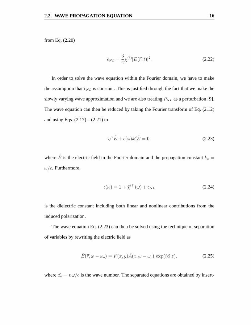
In order to solve the wave equation within the Fourier domain, we have to make
the assumption thatεNL is constant. This is justified through the fact that we make the
slowly varying wave approximation and we are also treatingPNL as a perturbation [9].
The wave equation can then be reduced by taking the Fourier transform of Eq. (2.12)
and using Eqs. (2.17) – (2.21) to
52E + ε(ω)k2oE = 0, (2.23)
whereE is the electric field in the Fourier domain and the propagation constantko =
ω/c. Furthermore,
ε(ω) = 1 + χ(1)(ω) + εNL (2.24)
is the dielectric constant including both linear and nonlinear contributions from the
induced polarization.
The wave equation Eq. (2.23) can then be solved using the technique of separation
of variables by rewriting the electric field as
E(~r, ω − ωo) = F (x, y)A(z, ω − ωo) exp(iβoz), (2.25)
whereβo = nω/c is the wave number. The separated equations are obtained by insert-

2.2. WAVE PROPAGATION EQUATION 17
ing Eq. (2.25) into Eq. (2.23), resulting in
d2F
dx2+
d2F
dy2+[ε(ω)k2
o − β2]F = 0, (2.26)
2iβodA(z)
dz+ (β2 − β2
o)A = 0, (2.27)
whereβ is the separation constant (eigenvalue). The equation for the modal distribution
F (r) can be solved by rewriting the dielectric constant as
ε = (n + δn)2 ≈ n2 + 2n δn. (2.28)
wheren is the index of refraction andδn is the nonlinear change of index as defined by
δn = n2 |E|2 +iα
2ko
=<e(εNL)
2n+
iα
2ko
. (2.29)
with n2 as the intensity-dependent index coefficient andα is the fiber loss coefficient.
To first order (neglecting the nonlinear contribution), Equation (2.26) reduces to a well-
known differential equation for the Bessel function by transforming to a cylindrical
coordinateF (x, y) = F (r) exp(imφ) and replacingε by n2,
d2F
dr2+
1
r
dF
dr+
[n2k2
o − β2 − m2
r2
]F = 0, (2.30)

2.2. WAVE PROPAGATION EQUATION 18
with the refractive indexn of a fiber of core radiusa given by
n =
n1 : r ≤ a
n2 : r > a(2.31)
The general solution in the core area of the fiber is the Bessel function consisting of a
linear combination of Bessel and Neumann functions and is given by
F (r) = Jm(κr), r ≤ a, (2.32)
with κ2 = n21k
2o − β2 since the Neumann function is non-physical because of a singu-
larity at r = 0 [9].
Equation (2.27) describes the propagation of the optical field within an optical fiber
and can be reduced by usingβ2 − β2o ≈ (β − βo)(β + βo) ≈ 2βo(β − βo). This is valid
by choosing the eigenvalueβ to be close toβo. Furthermore,β(ω) can be rewritten as
β(ω) = β(ω) + ∆β (2.33)
where∆β is the nonlinear contribution to the eigenvalue and can be calculated by using
the first-order perturbation theory. This is done by perturbing the system represented
by Eq. (2.26) by using Eqs. (2.28) and (2.33), and replacingF = F0 + δF . This results
in the following expression for∆β,
∆β =k0
∫ ∫∞−∞ δn |F (x, y)|2dx dy∫ ∫∞−∞ |F (x, y)|2dx dy
. (2.34)

2.2. WAVE PROPAGATION EQUATION 19
The propagation equation Eq. (2.27) then becomes
dA(z)
dz= i [β(ω) + ∆β − βo] A. (2.35)
2.2.1 Dispersion
Fiber dispersion is represented in Eq. (2.35) by the frequency dependent wave number
β(ω). We can expandβ(ω) in a Taylor series about the carrier frequencyωo as
β(ω) = βo + (ω − ωo)β1 +1
2(ω − ωo)
2β2 +1
6(ω − ωo)
3β3 + ..., (2.36)
with
βn =
(dnβ
dωn
)ω=ωo
. (2.37)
In order to study the propagation of the field in the time domain, we must perform the
inverse Fourier transform to Eq. (2.35) using the following relation
A(z, t) =1
2π
∫ ∞
−∞A(z, ω − ωo)e
−i(ω−ωo)tdω. (2.38)
The resulting time domain propagation equation including up to the second order effect
then becomes
∂A
∂z+ β1
∂A
∂t+
i
2β2
d2A
dt2= i∆βA. (2.39)

2.2. WAVE PROPAGATION EQUATION 20
Table 2.1: Parameters used in simulation of pulse broadening
Parameter Symbol ValuePulse shape A GaussianPulse width T0 10 psFiber dispersion β2 −10 ps2/kmDispersion length LD 10 km
First order fiber dispersionβ1 defines the group velocityvg of the pulse and second
order dispersionβ2, also known as group velocity dispersion (GVD), can cause pulse
spreading because different spectral components will experience different group ve-
locities. In studying pulse propagation, it is often convenient to measure time in the
moving frame of the pulse through the following transformation
T = t− β1z = t− z/vg. (2.40)
The resulting equation then becomes
∂A
∂z+
i
2β2
d2A
dT 2= i∆βA. (2.41)
A pulse launched into a dispersive medium usually does not maintain its shape and
can become a disruptive force in fiber-optic communications systems. As the pulse
is broadened its intensity degrades and crosstalk may develop with adjacent bit slots.
In general, we can define the dispersion lengthLD = T 2o /|β2| as the length in which
Gaussian pulse will spread to twice its initial pulse width,To. Figure 2.1 shows the
broadening of a Gaussian input pulse through one dispersion length assuming∆β = 0
using the parameters in Table 2.1.

2.2. WAVE PROPAGATION EQUATION 21
−50
5 0
5
10
0
0.2
0.4
0.6
0.8
1
Distance (km)
Normalized Time
Nor
mal
ized
pow
er
Figure 2.1: Pulse spreading due to GVD
2.2.2 Fiber Loss
Fiber loss is incorporated within the term∆β in Eq. (2.41). We can rewrite the prop-
agation constant in terms of index of refraction by noting that∆β = ko δn. Ignoring
the first term ofδn [Eq. (2.29)] for now (we will cover it in Section 2.2.3), substituting
Eqs. (2.29) and (2.34) into Eq. (2.41) results in
∂A
∂z+
i
2β2
d2A
dT 2= −α
2A. (2.42)
Fiber loss is a major problem in fiber-optic communication systems because of the loss
of signal power, which contributes directly to a high bit error rate. Figure 2.2 shows

2.2. WAVE PROPAGATION EQUATION 22
how the addition of fiber loss, in conjunction with fiber dispersion, can further degrade
the pulse intensity. The parameter used is the same as in Table 2.1 with the addition of
α = 0.2 dB/km.
−50
5 0
5
10
0
0.2
0.4
0.6
0.8
1
Distance (km)
Normalized Time
Nor
mal
ized
pow
er
Figure 2.2: Pulse spreading due to GVD in the presence of fiber loss
2.2.3 Nonlinear Schrodinger Equation
The nonlinear Schrodinger equation (NSE) is obtained by adding the intensity-
dependent index term to Eq. (2.42) by substituting both terms of Eqs. (2.29) and (2.34)
into Eq. (2.41),
∂A
∂z+
i
2β2
d2A
dT 2+
α
2A = iγ|A|2A, (2.43)

2.2. WAVE PROPAGATION EQUATION 23
where the nonlinear coefficientγ defined as
γ =ωo n2
c Aeff
, (2.44)
and the effective area defined as
Aeff =
(∫ ∫∞−∞ |F (x, y)|2dx dy
)2∫ ∫∞−∞ |F (x, y)|4dx dy
. (2.45)
By itself, nonlinearity can cause self-phase modulation (SPM) of the optical pulse.
SPM is caused by the intensity dependence of the index of refraction which causes a
time dependent nonlinear phase that leads to frequency chirp, a change of instantaneous
optical frequency across the pulse from its center valueωo. SPM induced chirp can
cause spectral broadening (see Fig. 2.3)which can lead to pulse compression. Similar
to the dispersion length, we can define a characteristic length of SPM (nonlinear length)
by
LNL =1
γPo
, (2.46)
wherePo is the peak power of the pulse.
There are other higher order nonlinear terms that we can add to the right hand side
of Eq. (2.43). In high bit-rate soliton systems that require the use of extremely short
optical pulses, a Raman effect on the pulse delay must be included in the nonlinear
Schrodinger equation [9]
∂A
∂z+
i
2β2
∂2A
∂T 2+
α
2A = iγ
[|A|2A− TR A
∂|A|2
∂T
]. (2.47)

2.3. OPTICAL SOLITONS 24
Table 2.2: Parameters used in simulation of pulse spectrum broadening
Parameter Symbol ValuePulse shape A Hyperbolic secantPulse width T0 10 psPulse power Ps 30 mWDispersion length LD 1000 kmNonlinear length LNL 10 km
2.3 Optical Solitons
We have seen in previous sections how fiber dispersion and fiber loss can distort the
shape of the pulse, which can have an adverse effect on signal propagation for commu-
nication purposes. However, if we were to use fiber nonlinearity to counter-balance the
fiber dispersion, a stable pulse can propagate undisturbed through the fiber — this is
the concept of optical solitons.
It is useful to normalize the nonlinear Schrodinger equation, Eq. (2.43), by intro-
ducing
U =A√Po
, ζ =z
LD
, τ =T
To
. (2.48)
The normalized nonlinear Schrodinger equation without the loss and the Raman term
is given by
∂U
∂ζ+
i
2sgn(β2)
∂2U
∂τ 2− iN2|U |2U = 0, (2.49)

2.3. OPTICAL SOLITONS 25
−1 −0.8 −0.6 −0.4 −0.2 0 0.2 0.4 0.6 0.8 10
0.1
0.2
0.3
0.4
0.5
0.6
0.7
0.8
0.9
1
Frequency (THz)
Nor
mal
ized
Pow
er
z = 0 km
z = 10 km
z = 20 km
z = 30 km
Figure 2.3: Spectral broadening of optical pulse due to SPM
whereN is the soliton order and is defined by
N2 =LD
LNL
=γPoT
2o
|β2|. (2.50)
Equation (2.49) can be solved by using the inverse scattering method [8] which consists
of choosing a suitable scattering problem whose potential is the solution sought. The
propagated field is reconstructed from the scattering data and the solution corresponds
to N = 1 is called the fundamental soliton and can be written as
U(ζ, τ) = sech(τ) exp
(iζ
2
). (2.51)

2.4. SPLIT-STEP FOURIER TRANSFORM METHOD 26
Table 2.3: Parameters used in simulation of soliton propagation
Parameter Symbol ValuePulse shape U SolitonSoliton order N 1Pulse width T0 10 psFiber dispersion β2 −10 ps2/kmDispersion length LD 10 kmNonlinear parameter γ 3.36 (W km)−1
Fiber loss α 0 dB/km
As can be seen readily from Eq. (2.50), whenN = 1, the dispersion lengthLD
exactly equals the nonlinear lengthLNL, indicating that the solution exists when fiber
nonlinearity exactly balances the fiber dispersion by choosing the appropriate launch
power for a given fiber dispersion and pulse width. This is not too surprising since we
have already seen how the pulse broadens due to GVD and compresses due to SPM.
Fig. 2.4 shows the stable propagation of a soliton pulse over a dispersion length without
any change in its shape using the parameters in Table 2.3.
2.4 Split-Step Fourier Transform Method
The inverse scattering method can solve the nonlinear Schrodinger equation only in
some specific cases. Numerical methods are employed to study the nonlinear effects in
optical fibers for most cases. Because of its speed, the most commonly used method
is the split-step Fourier transform method, which takes advantage of finite-Fourier-
transforms (FFT) algorithms [9].
The half-step Fourier transform methodology involves the separation of the equa-
tion into a differential partD to be solved in the Fourier domain and a nonlinear partN

2.4. SPLIT-STEP FOURIER TRANSFORM METHOD 27
−50
5 0
5
10
0
0.2
0.4
0.6
0.8
1
Distance (km)
Normalized Time
Nor
mal
ized
pow
er
Figure 2.4: Soliton pulse propagation
to be solved in the time domain. This can be written mathematically as
∂A
∂z= (D + N)A, (2.52)
where the operators are given by
D = − i
2β2
∂2A
∂T 2− α
2, (2.53)
N = iγ|A|2 + other nonlinear terms. (2.54)
The assumption made in using the split-step Fourier transform method is that even
though dispersion and nonlinearity act concurrently over a small distanceh, the dis-

2.4. SPLIT-STEP FOURIER TRANSFORM METHOD 28
persive and nonlinear effects can be assumed to act separately. The method is imple-
mented by applying only the dispersive effect on the first half of the step, then applying
the nonlinearity for the whole step (assuming the power is approximately constant over
the step size,h), and finally re-applying the dispersive effect on the second half of the
step. This is also referred to as the symmetric split-step Fourier transform method, (see
Figure 2.5). Note that since the dispersion operatorD consists of differential operator,
Figure 2.5: Split-step Fourier transform method
it is solved easily in the Fourier domain by using FFT. Mathematically, the numerical
methodology can be given by the following equation
A(z + h, T ) = exp
(D
h
2
)exp(Nh) exp
(D
h
2
)A(z, T ). (2.55)
The accuracy of the symmetric split-step Fourier transform method can be estimated
by comparing the exact solution to the approximated solution. If we assume thatN is

2.5. VARIATIONAL TECHNIQUE 29
independent of z, the exact solution is given by
A(z + h, T ) = exp((D + N)h
)A(z, T ). (2.56)
A comparison of the exact solution [Eq. (2.56)] with the approximate solution
[Eq. (2.55)] using the Baker-Hausdorff formula shows that the error is on the order
of h3 [9].
2.5 Variational Technique
The propagation of soliton pulses in each fiber section between two consecutive ampli-
fiers is described by the nonlinear Schrodinger equation, Eq. (2.49). The loss term can
be eliminated with the following change of variables
A = B exp(−αz/2), γ(z) = γ0 exp(−αz), (2.57)
whereγ0 is the nonlinear coefficient in the absence of loss. This reduces the nonlinear
Schrodinger equation into the following form:
i∂B
∂z− 1
2β2
∂2B
∂T 2+ γ(z)|B|2B = 0. (2.58)
The effects of fiber loss are now included through thez dependence ofγ.
Variational analysis provides approximate analytical results for features such as
pulse compression, maximal pulse amplitude, and induced frequency chirp [20]. The
nonlinear Schrodinger equation can be restated as a variational problem by casting it in

2.5. VARIATIONAL TECHNIQUE 30
the form of the Euler-Lagrange equation
∂
∂z
(∂L
∂qz
)+
∂
∂T
(∂L
∂qT
)− ∂L
∂q= 0, (2.59)
whereq represents the fieldB or B∗, the subscriptsT andz denote differentiation with
respect to the appropriate variable, and the Lagrangian densityL is given by [20]
L = − i
2(B∗Bz −BB∗
z )−1
2
[γ(z)|B|4 + β2|BT |2
], (2.60)
where a subscript denotes derivative with respect to that variable. Note that combining
Eqs. (2.59) and (2.60) withq = B∗ produces Eq. (2.58).
To carry out the variational analysis, we average the Lagrangian density by integrat-
ing over time
L =
∫ ∞
−∞L[T, q(z)] dT. (2.61)
Integrating Eq. (2.59) over time, the reduced Euler-Lagrange equation becomes
d
dz
(∂L∂qz
)− ∂L
∂q= 0. (2.62)
To make further progress, we choose the following ansatz for the soliton shape and
phase:
B(z, T ) = a sech
(T
To
)exp
(iφ− iCT 2
2T 2o
), (2.63)
wherea is the amplitude,φ is the phase,C is the chirp, andTo is the pulse width. All

2.5. VARIATIONAL TECHNIQUE 31
of the soliton parameters exceptφ remain constant for a lossless fiber but are allowed
to vary withz when solitons are amplified periodically to compensate for fiber losses.
Performing the integral in Eq. (2.61) gives the following expression for the average
Lagrangian density
L = a2
(2φzTo −
π2
12CzTo +
π2
6CToz
)− 2
3γ(z)a4To −
β2a2
3To
(1 +
π2
4C2
). (2.64)
By combining Eqs. (2.62) and (2.64) withq representing any of the variablesa, To,
C, or φ, we obtain the following set of four ordinary differential equations governing
variations of soliton parameters along the fiber link:
d(a2To)
dz= 0, (2.65)
dTo
dz=
β2C
To
, (2.66)
dC
dz=
4
π2γ(z)a2 +
β2
T 2o
(4
π2+ C2
), (2.67)
dφ
dz=
β2
3T 2o
+5
6γ(z)a2. (2.68)
These equations are equivalent to solving the nonlinear Schrodinger equation within
the variational approximation. Note however, that this approach is only approximate
and does not account for characteristics such as radiative loss [21], damping of the
amplitude oscillations, and changing of soliton shape [20]. It should be stressed that
Eqs. (2.65) – (2.68) can also be applied for dispersion-managed solitons by makingβ2
explicitly z-dependent. In the next chapter, we consider the case of constant-dispersion
fibers first.

2.6. SUMMARY 32
2.6 Summary
In this chapter, we presented the theory for nonlinear pulse propagation based on
Maxwell’s equations taking into account fiber dispersion, fiber losses, and fiber non-
linearity. We have also presented the optical soliton as a solution to the nonlinear
Schrodinger equation that can be used advantageously in fiber optic communication
systems. An efficient numerical algorithm is presented to effectively study the nonlin-
ear pulse propagation. Furthermore, we presented the foundation of the variational
method as an effective analytical tool in studying nonlinear propagation dynamics.
This technique will be crucial in providing analytic insight in studying periodicity of
constant-dispersion (Chapter 3) as well as dispersion-managed systems (Chapter 5).

33
Chapter 3
Chirped Solitons inConstant-Dispersion Fiber Links
3.1 Introduction
We introduced the concept of optical solitons in section 2.3 for transmitting information
in an optical communication system. The ability of the soliton to maintain its shape as
it propagates through an optical fiber, a dispersive and nonlinear medium, makes it an
ideal choice in transmitting signals. Unfortunately, fiber loss reduces the nonlinearity
needed to balance fiber dispersion, and a soliton can no longer be preserved. Optical
amplifiers were developed to mitigate the problem of fiber loss and have been very
successful. Lumped amplification systems place optical amplifiers periodically along
the fiber link to compensate for the fiber loss. For cost effectiveness, it is necessary to
have as large an amplifier spacing or conversely, as few amplifiers as possible.
The principal concept that has emerged in the context of lumped amplification is
the path-averaged or guiding-center soliton [22–24]. This allows propagation of soli-
tons through lossy fibers provided the amplifier spacingLA is short compared to the
dispersion lengthLD. The soliton is launched with enough energy such that the path-

3.2. GUIDING-CENTER SOLITONS 34
averaged peak power over one amplifier spacing is equal to the peak power needed
for soliton propagation. However, this results in the need to limitLA to a fraction
of LD (LA � LD), which in turn necessitates unreasonably short amplifier spacings
(< 10 km) when operating at high bit rates. This limitation comes from the fact that the
system is not perfectly periodic whenLA becomes comparable to or exceedsLD. As a
result, large perturbations generate spectral side bands and dispersive radiation which
degrade the system performance [25–27]. Several techniques have been proposed to de-
sign soliton communication systems that can operate beyond the average-soliton regime
[28–31]. However, their use often requires additional optical elements such as a fast sat-
urable absorber [9]. We propose a way to extend the amplifier spacing to beyond the
guiding-center soliton through pulse prechirping.
3.2 Guiding-Center Solitons
The normalized nonlinear Schrodinger equation including the effect of periodic optical
gain provided by a series of inline optical amplifiers can be written as [2]
∂U
∂ζ+
i
2sgn(β2)
∂2U
∂τ 2− iN2|U |2U = −Γ
2U +
(√G− 1
) N∑n=1
δ(ζ − nzA)U, (3.1)
whereΓ = γLD is the normalized loss coefficient,G = exp(Γ zA) is the amplifier
gain, andzA is the normalized amplifier length for the fundamental soliton (N = 1)
in a anomalous dispersion fiber (β2 < 0). Similar to the slowly varying envelope
approximation of the previous chapter, we will separate the fast varying function that
describes the soliton losses and amplifications (a) and the slowly varying function of
the dispersion and nonlinear effect (u). The optical field can then be written as the
3.2. GUIDING-CENTER SOLITONS 35
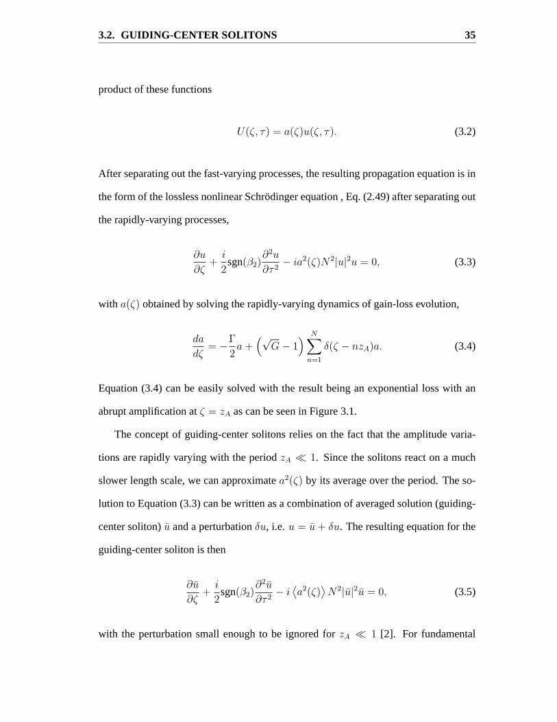
product of these functions
U(ζ, τ) = a(ζ)u(ζ, τ). (3.2)
After separating out the fast-varying processes, the resulting propagation equation is in
the form of the lossless nonlinear Schrodinger equation , Eq. (2.49) after separating out
the rapidly-varying processes,
∂u
∂ζ+
i
2sgn(β2)
∂2u
∂τ 2− ia2(ζ)N2|u|2u = 0, (3.3)
with a(ζ) obtained by solving the rapidly-varying dynamics of gain-loss evolution,
da
dζ= −Γ
2a +
(√G− 1
) N∑n=1
δ(ζ − nzA)a. (3.4)
Equation (3.4) can be easily solved with the result being an exponential loss with an
abrupt amplification atζ = zA as can be seen in Figure 3.1.
The concept of guiding-center solitons relies on the fact that the amplitude varia-
tions are rapidly varying with the periodzA � 1. Since the solitons react on a much
slower length scale, we can approximatea2(ζ) by its average over the period. The so-
lution to Equation (3.3) can be written as a combination of averaged solution (guiding-
center soliton)u and a perturbationδu, i.e. u = u + δu. The resulting equation for the
guiding-center soliton is then
∂u
∂ζ+
i
2sgn(β2)
∂2u
∂τ 2− i⟨a2(ζ)
⟩N2|u|2u = 0, (3.5)
with the perturbation small enough to be ignored forzA � 1 [2]. For fundamental

3.2. GUIDING-CENTER SOLITONS 36
0 2 4 6 8 10 12 14 16 18 200.6
0.65
0.7
0.75
0.8
0.85
0.9
0.95
1
Distance (km)
Pow
er (
norm
aliz
ed)
Figure 3.1: Amplitude variations of lumped amplification withLA=20 km and 0.2 dB/km loss.
solitons to operate in the guiding-center soliton, input peak power of the pulse should
be given such that〈a2(ζ)〉N2 = 1. For amplifier gain equal to fiber loss over the
amplifier span, the peak power is given as
Pin =G ln G
G− 1P0, (3.6)
whereP0 is the power required for the fundamental soliton in a lossless fiber. Figure
3.2 shows the evolution of a guiding center soliton through two amplifier stages with
zA = 0.2 (see Table 3.1). The figure clearly illustrates the effect of fiber loss which

3.3. PRE-CHIRPED SOLITONS 37
Table 3.1: Parameters used in simulation of soliton propagation
Parameter Symbol ValuePulse shape U SolitonSoliton order N 1.117Pulse width T0 10 psFiber dispersion β2 −2 ps2/kmDispersion length LD 50 kmNonlinear parameter γ 3.36 (W km)−1
Fiber loss α 0.2 dB/kmAmplifier spacing LA 10 km
causes pulse broadening but it also shows the ability of the pulse to retain its soliton
nature through periodic amplification.
3.3 Pre-Chirped Solitons
A question one may ask is whether the periodicity of solitons (see Figure 3.3) can be re-
stored even whenLA ∼ LD by modifying the system design in an appropriate way. For
example, the guiding-center soliton is launched with an unique peak power obtained
by averaging the soliton energy over one amplifier spacing. However, the soliton is as-
sumed to remain unchirped [22,32]. The trick is then to allow both the width and chirp
of the soliton to vary in each fiber section between two amplifiers (similar concepts
have been used in dispersion-managed solitons [33–38]). We use variational analy-
sis to determine the optimal launch conditions for the guiding-center soliton (GCS)
or path-averaged soliton (PAS). We require the pulse width and chirp to be periodic
and determine the exact pre-chirping and peak power needed to maintain periodicity
of soliton in periodically amplified fiber links. The use of prechirping provides a new

3.3. PRE-CHIRPED SOLITONS 38
−50
5 0
10
20
0
0.2
0.4
0.6
0.8
1
Distance (km)
Normalized Time
Nor
mal
ized
pow
er
Figure 3.2: Evolution of guiding-center soliton
operating regime for such systems in whichLA can be comparable and even exceed
LD. This regime is especially useful at high bit rates (B > 10 Gb/s) for which the
dispersion length becomes∼ 10 km. Furthermore, even though we focus on the case of
constant-dispersion fibers, the new regime discussed here may find applications in the
case of dispersion-managed lightwave systems.
3.3.1 Variational Results
Equation (2.65) shows the conservation of pulse energyEp =∫|B|2 dt and relates the
amplitudea of the pulse to its widthTo. We can write the relation asa2 = a20To(0)/To
wherea0 andTo(0) are the initial pulse amplitude and width, respectively. As a result,

3.3. PRE-CHIRPED SOLITONS 39
Figure 3.3: Periodicity of soliton pulse through each amplifier unit
φ is strictly determined byTo, and the variational analysis is reduced to solving a pair of
coupled ordinary differential equations forC andTo only [Eq. (2.66) and (2.67)]. Fur-
thermore, it is useful to introduce the normalized lengthξ = z/LA, and the normalized
pulse widthW = To/To(0). Equation. (2.66) and (2.67) then become
dW
dξ= −zAC
W, (3.7)
dC
dξ=
4zAP0 exp(−Γξ)
π2W− zA
W 2
(4
π2+ C2
). (3.8)
whereΓ = αLA, andP0 = γ0 a20 LD is the normalized initial peak power. Our objec-
tive is to find a periodic solution of Eqs. (3.7) and (3.8) such that all soliton parameters
(exceptφ) recover their initial values after one amplifier spacing. This periodicity con-
dition can only be met under certain launch conditions. The optimal launch conditions
are determined by solving Eqs. (3.7) and (3.8) with the boundary conditions
C(0) = C0 = C(1), W (0) = 1 = W (1). (3.9)

3.3. PRE-CHIRPED SOLITONS 40
3.3.2 Analytical Results
In general, Eqs. (3.7)–(3.9) should be solved numerically by considering different in-
put values for the peak powerP0, pulse widthTo(0), and initial chirpC0. Because of
the multidimensional nature of the parameter space, an exhaustive search for periodic
solutions is quite time consuming. However, we can solve Eqs. (3.7) and (3.8) approx-
imately by using a perturbation method in the regimezA << 1. The natural parameter
for perturbation expansion iszA sinceC andW vary little along the fiber length for
zA << 1. ExpandingC andW up to second-order inzA, we can write
W = W0 + W1zA + W2z2A, (3.10)
C = C0 + C1zA + C2z2A. (3.11)
SinceC0 = 0 andW0 = 1 (the lossless case), we obtain the following two equations
by substituting Eq. (3.10) and (3.11) into Eq. (3.7) and (3.8) and collecting the terms in
similar powers ofzA,
dW2
dξ= −C1, (3.12)
dC1
dξ=
4P0 exp(−Γξ)
π2− 4
π2. (3.13)
The width parameterW has no first-order corrections. These equations can be solved
by direct integration to obtainC1(ξ) and W2(ξ). Applying the boundary condition
C1(0) = C1(1) sets the launch condition for peak power to be
P0 =Γ
1− exp(−Γ)=
G ln G
G− 1. (3.14)

3.4. NUMERICAL RESULTS 41
Similarly, applying the boundary conditionW2(0) = W2(1) provides the input chirp
C1(0) =2
π2−(
4
π2
)exp(−Γ) + Γ− 1
Γ(1− exp(−Γ))
=4
π2
[1
2+
(G− 1)−G ln G
ln G(G− 1)
]. (3.15)
The peak-power condition, Eq. (3.14), is the same as that obtained by the guiding-center
soliton theory [22] (also see Eq. (3.6)) assuming that an unchirped soliton is launched at
the input end. The chirp condition, Eq. (3.15), is new and is obtained by requiring that
the pulse width recovers its initial value periodically. We have seen that the variational
analysis allows us to examine the conditions of periodicity for both the chirp and the
width, resulting in an additional constraint in Eq. (3.15). We will refer these solitons as
chirped path-average solitons.
3.4 Numerical Results
In this section we discuss the new operating regime of chirped solitons and compare it
with the standard operating regime in which unchirped solitons are launched at the input
end. The perturbation analysis of Section 3.3.1 provides an estimate of the launching
parameter only forzA << 1. However, we expect on physical grounds chirped solitons
to be useful for designing high-speed periodically amplified fiber links even whenzA
exceeds 1. The operating region in which the amplifier spacing is comparable or larger
than the dispersion length (zA > 1) can be studied by solving Eqs. (3.7) and (3.8)
numerically.
To obtain the numerical solution, we use a root-finding algorithm to satisfy the
boundary conditions imposed by Eq. (3.9). For definiteness, we chooseLA = 40 km
3.4. NUMERICAL RESULTS 42
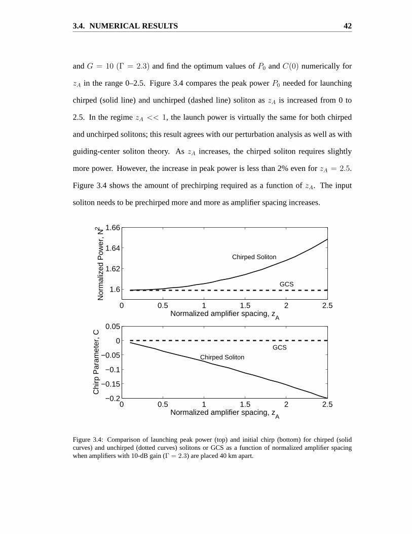
andG = 10 (Γ = 2.3) and find the optimum values ofP0 andC(0) numerically for
zA in the range 0–2.5. Figure 3.4 compares the peak powerP0 needed for launching
chirped (solid line) and unchirped (dashed line) soliton aszA is increased from 0 to
2.5. In the regimezA << 1, the launch power is virtually the same for both chirped
and unchirped solitons; this result agrees with our perturbation analysis as well as with
guiding-center soliton theory. AszA increases, the chirped soliton requires slightly
more power. However, the increase in peak power is less than 2% even forzA = 2.5.
Figure 3.4 shows the amount of prechirping required as a function ofzA. The input
soliton needs to be prechirped more and more as amplifier spacing increases.
0 0.5 1 1.5 2 2.5
1.6
1.62
1.64
1.66
Nor
mal
ized
Pow
er, N
2
Normalized amplifier spacing, zA
0 0.5 1 1.5 2 2.5−0.2
−0.15
−0.1
−0.05
0
0.05
Normalized amplifier spacing, zA
Chi
rp P
aram
eter
, C
Chirped Soliton
GCS
GCS
Chirped Soliton
Figure 3.4: Comparison of launching peak power (top) and initial chirp (bottom) for chirped (solidcurves) and unchirped (dotted curves) solitons or GCS as a function of normalized amplifier spacingwhen amplifiers with 10-dB gain (Γ = 2.3) are placed 40 km apart.

3.4. NUMERICAL RESULTS 43
The need for negative prechirping can be understood by examining Eq. (3.8), which
shows thatdC/dξ contains a negative term (sinceβ2 < 0 for anomalous dispersion)
and an exponentially decreasing positive term. Initially, the positive term dominates
due to the high peak power, and the chirp increases with propagation. However, the
nonlinear term is reduced because of fiber loss, anddC/dξ becomes negative, resulting
in a downward concave trajectory. In addition the boundary condition Eq. (3.9) requires
that
∫ 1
0
C(ξ) dξ = 0. (3.16)
For a concave-down trajectory this integral relation can be satisfied only for negatively
prechirped pulses [C(0) < 0] [see figure 3.6(b)].
Since both the soliton width and chirp are allowed to vary alongz periodically in the
new operating regime proposed here, it is important to consider the extent of variation
in each fiber section between two amplifiers. Figures 3.5 and 3.6 show variation of
pulse width and chirp along the fiber length forzA = 0.4 andzA = 2.1 respectively
using launch conditions corresponding to a chirped (solid line) and an unchirped soliton
(dashed line).
In the zA << 1 regime, the chirp is fairly periodic in both cases. But since the
unchirped soliton does not impose periodicity of the pulse width, soliton width is re-
duced by 1%. In contrast, the width recovers its initial value for the chirped soliton.
In thezA > 1 regime, however, the perturbation becomes too great for the unchirped
soliton to maintain the periodic nature of the pulse width and chirp. As seen in Fig-
ure 3.6(a), the soliton width can vary as much as by 20% (dashed line) and is smaller
by 10% after one amplifier spacing. In contrast, the chirped PAS recovers both pulse

3.4. NUMERICAL RESULTS 44
Figure 3.5: Evolution of pulse width and chirp over one amplifier stage for a chirped (solid curves) andan unchirped (dotted curves) soliton or GCS as predicted by variational analysis. Normalized amplifierspacing iszA = 0.4.
width and chirp after each amplifier. Also, width variations are much smaller (< 5%)
for chirped solitons showing clearly that such solitons are not perturbed significantly
even whenzA > 1.
In order to check the validity of variational analysis, Figure 3.7 and 3.8 are obtained
using the same parameters as those used in Figure 3.5 and 3.6 except that the nonlinear
Schrodinger equation is solved numerically over 20 amplification stages (total trans-
mission distance of 800 km). The root-mean-square (RMS) width [2] (see Appendix)
and chirp of the pulse are calculated numerically. We decided to estimate the RMS
width since the shape of the pulse is not guaranteed to remain preserved even though
variational analysis requires it. The chirp parameter is estimated by fitting a parabola
to the phase profile in the vicinityT = 0 and noting from Eq. (2.63) that the quadratic
term varies asCT 2/2T 2o . Figure 3.7 and 3.8 show that the periodicity inC andTo

3.4. NUMERICAL RESULTS 45
Figure 3.6: Evolution of pulse width and chirp over one amplifier stage for a chirped (solid curves) andan unchirped (dotted curves) soliton or GCS as predicted by variational analysis. Normalized amplifierspacing iszA = 2.1.
is maintained only approximately over multiple amplifiers. For example, RMS pulse
width varies1% from amplifier to amplifier whenzA = 0.4, and variations become as
large as10% whenzA = 2.1. This is not surprising and indicates that the “sech” pulse
shape is not the true pulse shape for the periodic solution of the nonlinear Schrodinger
equation . As we noted earlier, variational analysis cannot accurately predict the soli-
ton parameters once the shape of the soliton is not preserved. Figures 3.7(a) and 3.8(a)
show that the RMS width varies less when a chirped soliton is launched. For instance,
in the casezA = 2.1, width of unchirped solitons exhibit more than20% variation,
whereas chirped solitons exhibit a maximum of10% variation. This feature suggests
that, in general, the use of prechirped solitons is likely to provide better system perfor-
mance compared with unchirped solitons.
To explore the soliton-stability issue, we have plotted the chirp and width variations

3.4. NUMERICAL RESULTS 46
Figure 3.7: Same as in Fig. 3.5 except that soliton evolution over 20 amplification stages (total distanceof 800 km) is shown by solving the NSE numerically.
in the two-dimensional phase space as a Poincare map since such a map shows the
phase-space region over which width and chirp vary along the fiber length. Figure 3.9
shows the Poincare map for chirped and unchirped solitons over 100 amplifier spacing
(4000 km). Ideally, if the system is perfectly periodic, we would expect all the points
to coincide, resulting in a single dot in the plot. Our numerical results show that for
both zA = 0.4 and zA = 2.1, the chirped soliton is more localized, implying that
both the soliton width and chirp vary over a smaller range from one amplifier to the
next. This behavior confirms our variational result that prechirping is necessary for
stable propagation. Forysiaket al. [30] reached a similar conclusion using an operator-
splitting technique.

3.5. SUMMARY 47
Figure 3.8: Same as in Fig. 3.6 except that soliton evolution over 20 amplification stages (total distanceof 800 km) is shown by solving the NSE numerically.
3.5 Summary
Fiber-optic communication systems employ the technique of lumped amplification to
compensate for fiber losses. In order to maintain soliton integrity in the presence of
fiber losses, guiding-center soliton is used but the system is then limited in the am-
plifier spacing it can sustained. We have found a new operating regime for soliton
transmission in periodically amplified lightwave systems. This regime requires launch-
ing of an initially chirped soliton. Our variational analysis recovers the guiding-center
soliton result in the regimezA << 1. By allowing both the pulse width and the chirp
to vary over each amplifier section, we find that prechirping the pulse is necessary in
order to sustain path-averaged solitons in the regimezA ∼ 1 in a periodically amplified
optical communication system. We use the results of variational analysis to determine
the amount of pre-chirping and initial peak power required to recover initial launch val-

3.5. SUMMARY 48
Figure 3.9: Poincare map obtained by plotting soliton width and chirp at the end of each amplifier sectionfor 100 amplification stages (4000 km) for unchirped or GCS (*) and chirped (•) soliton. ForzA = 0.4,nearly circular compact region shows the quasi-periodic nature of soliton evolution. ForzA = 2.1,soliton width and chirp vary over a wider region.
ues at each amplifier. Numerical solutions of the nonlinear Schrodinger equation show
that the use of prechirped solitons improves stability since variations of pulse width and
chirp over a large transmission distance are much smaller compared to guiding-center
solitons. The new operating regime should be useful at high bit rates (> 20 Gb/s) by
permitting amplifier spacing to become larger than the dispersion length. This tech-
nique is simple to implement because most pulses emitted by semiconductor lasers are
chirped. In addition, correct prechirping can also be achieved through propagating the
pulse through a correct length of optical fiber.

49
Chapter 4
Distributed Amplification inConstant-Dispersion Systems
4.1 Introduction
Soliton communication systems are leading candidates for long-haul lightwave trans-
mission links because they offer the possibility of a dynamic balance between group-
velocity dispersion (GVD) and self-phase modulation (SPM), the two effects that
severely limit the performance of non-soliton systems [2,39]. Most system experiments
employ the technique of lumped amplification and place fiber amplifiers periodically
along the transmission line for compensating the fiber loss.
The limitation on the amplifier spacing imposed by lumped amplification was stud-
ied (see guiding-center soliton, section 3.2). This limitation can be overcome by
prechirping the pulse (see Chapter 3) or by using distributed amplification [14]. In this
scheme [40,41], the transmission fiber is pumped periodically, creating sufficient gain
through either the presence of rare-earth erbium ions or using stimulating Raman scat-
tering (SRS) for compensating the fiber loss. Since the gain is distributed throughout
the fiber link and compensate the fiber loss locally all along the fiber, soliton peak-

4.2. ERBIUM-DOPED FIBER AMPLIFIERS 50
power variations can be made much smaller compared with the lumped amplification
scheme. Although one expects the pump-station spacingLA to become comparable
and even exceedLD in the case of distributed amplification, a systematic comparison
of the lumped and distributed amplification schemes is not available in the literature.
Furthermore, shorter pulses needed at high bit rates are affected considerably by SRS,
therefore the inclusion of SRS is essential in modeling high-bit-rate systems [9].
4.2 Erbium-Doped Fiber Amplifiers
Fiber-optic communication systems compensates for fiber losses through the use of
EDFAs. An EDFA consists of regular silica fiber doped with erbium rare earth ions and
is modeled as a three-level gain medium (see Figure. 4.1). Semiconductor lasers are
4.2. ERBIUM-DOPED FIBER AMPLIFIERS 43
the pump-station spacingLA to become comparable and even exceedLD in the case of
distributed amplification, a systematic comparison of the lumped and distributed ampli-
fication schemes is not available in the literature. Furthermore, shorter pulses needed
at high bit rates are affected considerably by SRS, therefore the inclusion of SRS is
essential in modeling high-bit-rate systems [12].
4.2 Erbium-Doped Fiber Amplifiers
4.2.1 Introduction
Fiber-optic communication systems compensates for fiber loss through the use of
EFDA. EDFA consisted of regular silica fiber doped with erbium rare earth ions can
be modeled as a three-level gain medium (see Figu. 4.2.1). Semiconductor lasers are
10/19/99ZML:IAF99 8
Lightly doped fiber
Modeling d-EDFA
Signal
Pump BeamP1 P2
N3
N2
N1
WpN1
WN2
[ ] 111 )( PzNzP
ασ −−=∂∂
[ ] 212 )( PzN
zP
ασ −−−=∂∂
),()( Tp NWNzg ∆⋅= σ
21 PPWp +∝ sPW ∝
[ ]
−∫ dzzgAL
0
)(min α
Figure 4.1: Three level model of erbium-doped gain mediumFigure 4.1: Three level model of erbium-doped gain medium
usually used as pump power sources to provide the population inversion necessary to
achieve gain.

4.2. ERBIUM-DOPED FIBER AMPLIFIERS 51
The rate equations for the three level system can be written down as follows:
dN3
dt= WpN1 −N3γ3 −WpN3 (4.1)
dN2
dt= N3γ3 −W (N2 −N1)−N2γ2 (4.2)
dN1
dt= N2γ2 + W (N2 −N1)−Wp(N1 −N3), (4.3)
WhereN1, N2, andN3 are the number of erbium ions in each of the respective energy
levels, andNT = N1 + N2 + N3 is the total number of erbium ions (ions/µm3) in the
fiber. The relaxation rate of the energy states (second and third level) are represented
by γ2 andγ3 respectively,W andWp are the photon density rates of the signal and the
pump. The steady state solution ofdNi
dt= 0 (where i=1, 2, 3) reduces the rate equations
(4.1) – (4.3) to the following equalities:
N1 =N3(γ3 + Wp)
Wp
≈ N3γ3
Wp
(4.4)
N2 =N3γ3 + WN1
W + γ2
≈ N1(W + Wp)
W + γ2
(4.5)
N3 =N1(Wp + W )−N3Wp
W + γ2
≈ N1(Wp + W )
W + γ2
, (4.6)
with the assumption that the third level decays faster than the pump absorption (γ3 �
Wp), and most of the ions are going to be in the ground state as compared to the upper
state (N1 � N3). The population inversion∆N can then be calculated from the above
equations using∆N = N2 −N1
∆N =NT (γ3Wp − γ3γ2 −Wpγ2)
W (3Wp + 2γ3) + 2Wpγ2 + γ3(Wp + γ2). (4.7)

4.2. ERBIUM-DOPED FIBER AMPLIFIERS 52
For a rapid upper state relaxation (γ3 � γ2, Wp), Eq. (4.7) can be further reduced to
∆N =NT (Wp − γ2)
2W + Wp + γ2
. (4.8)
The gain of the medium is the product of the absorption cross section and the population
inversion so that
g = σ∆N =σNT (Wp − γ2)
2W + Wp + γ2
. (4.9)
Lumped amplification schemes using EDFA necessitates that the net gain of the ampli-
fier exactly compensates for the fiber loss. To this end, the fiber is doped heavily and
Eq. (4.9) is solved with respect to pump rateWp such that sufficient gain is obtained,
the stipulation being of course that the amplifier lengthLA obeys the guiding-center
soliton condition of section 3.2 or the prechirped path-average condition of section 3.3.
Even though the amplifier is intended to amplify a train of optical pulses, the com-
munication system operates at very high bit rates with pulses in the order of picoseconds
and because the fluorescence lifetime of the excited erbium ions is only order of≈ 10
ms, we can write the signal and pump waves in the continuous wave (CW) regime [2].
The equations that describe the pump-signal interaction are given as
dPp
dz= −(σpN1 + αp)Pp, (4.10)
dPs
dz= (σs∆N − αs) Ps. (4.11)
wherePp, Ps, σp, andσs are the pump and signal powers and transition cross sections
respectively. The above equations are used to study the small-signal and large-signal

4.3. DISTRIBUTED ERBIUM-DOPED FIBER AMPLIFIERS 53
amplification and their predictions are accurate for our purposes. The gain of EDFA can
be as high as 30 dB with only 30 m of erbium-doped fiber requiring only approximately
4 mW of pump power at 1.48µm [2].
4.3 Distributed Erbium-Doped Fiber Amplifiers
Distributed erbium-doped fiber amplifiers (d-EDFA) basically replace the traditional
set of transmission fiber and high-gain EDFA with a transmission fiber that is lightly
doped with rare-earth erbium ions. The link then becomes essentially transparent when
pumped from both directions (see Figure 4.2). Fiber transparency can be accomplished
with various dopant concentrations, which can be used to adjust for minimum gain/loss
perturbation for the soliton pulses.
Figure 4.2: Distributed-erbium doped amplifier link
4.3.1 Modeling Gain in Distributed Fiber Amplifiers
Since d-EDFA is just an extension of EDFA, we can use the same three-level gain model
from the previous section (Sec. 4.2). Since the erbium-doped fiber length is much

4.3. DISTRIBUTED ERBIUM-DOPED FIBER AMPLIFIERS 54
longer and we are trying to minimize gain/loss perturbation, the optimal pump scheme
consists of bi-directional pumping [42] (see Fig. 4.3). We can study the evolution of
4.2. ERBIUM-DOPED FIBER AMPLIFIERS 43
the pump-station spacingLA to become comparable and even exceedLD in the case of
distributed amplification, a systematic comparison of the lumped and distributed ampli-
fication schemes is not available in the literature. Furthermore, shorter pulses needed
at high bit rates are affected considerably by SRS, therefore the inclusion of SRS is
essential in modeling high-bit-rate systems [12].
4.2 Erbium-Doped Fiber Amplifiers
4.2.1 Introduction
Fiber-optic communication systems compensates for fiber loss through the use of
EFDA. EDFA consisted of regular silica fiber doped with erbium rare earth ions can
be modeled as a three-level gain medium (see Figu. 4.2.1). Semiconductor lasers are
10/19/99ZML:IAF99 8
Lightly doped fiber
Modeling d-EDFA
Signal
Pump BeamP1 P2
N3
N2
N1
WpN1
WN2
[ ] 111 )( PzNzP
ασ −−=∂∂
[ ] 212 )( PzN
zP
ασ −−−=∂∂
),()( Tp NWNzg ∆⋅= σ
21 PPWp +∝ sPW ∝
[ ]
−∫ dzzgAL
0
)(min α
Figure 4.1: Three level model of erbium-doped gain medium
Figure 4.3: Bi-directional pumping of d-EDFA
forward and backward pump powers along with the signal power using the following
set of three equations.
dPf
dz= [−A N1(z; Pf , Pb)− αp]Pf , (4.12)
dPb
dz= [A N1(z; Pf , Pb) + αp]Pb, (4.13)
dPs
dz= [σ ∆N(z; Pf , Pb)− αs]Ps. (4.14)
which include the saturation of gain as well as pump depletion.Pf , Pb, andPs are the
forward, backward-pump and signal powers respectively.
4.3.2 Small-Signal Solution
Assuming small signal power, we can solve the above equations analytically by ignor-
ing the first term in the pump power equation that represents the pump depletion due
to absorption. Just keeping the fiber loss term of the pump powers, the forward and

4.3. DISTRIBUTED ERBIUM-DOPED FIBER AMPLIFIERS 55
backward pumped powers are given as
Pf (z) = Pi exp(−αp z), (4.15)
Pb(z) = Pi exp[αp(z − LA)], (4.16)
wherePi is the initial pump power. The saturation power can be written in terms of
the pump powers by noting that the signal and pump rate can be rewritten in terms of
power
W =σ P
Eo Aeff
. (4.17)
Eq. (4.9) can then be rewritten as
g =go
1 + Ps/Psat
, (4.18)
where the small signal gaingo and the saturation power are define as
go =σ Nt(Pf + Pb + PA)
Pf + Pb + PA
, (4.19)
Psat =1
2(Pf + Pb + PA) , (4.20)
wherePA = Eo Aeffγ2/σ represents the spontaneous emission, which contributes to
the noise of the system.

4.3. DISTRIBUTED ERBIUM-DOPED FIBER AMPLIFIERS 56
4.3.3 Numerical Solution
Full solution can be obtained numerically by integrating Eqs. (4.12)–(4.14). Further
simplification can be applied to reduce the complexity of the problem by noting that
Eqs. (4.12)–(4.13) have the following equality
− 1
Pf
dPf
dz=
1
Pb
dPb
dz. (4.21)
Simple algebraic manipulation yields the following relation between the forward and
backward pump powers
d
dz[ln(Pf ) + ln(Pb)] = 0,
d
dz(Pf + Pb) = 0,
Pf Pb = C, (4.22)
where C is a constant that is the product of the forward and backward pump-powers.
To summarize, the following constrains are used to solve coupled ordinary differential
equations given by Eqs. (4.12)–(4.14):
Pf Pb = C, (4.23)
Pf (z = 0) = Pb(z = LA), (4.24)∫ LA
o
g(z)− αs dz = 0. (4.25)
Figure 4.4 shows the comparison between the analytical and numerical solution of
the pump power evolution, showing the role of pump absorption on a 100 km d-EDFA

4.3. DISTRIBUTED ERBIUM-DOPED FIBER AMPLIFIERS 57
amplifying an averaged signal power of 0.3 mW with losses of 0.2 dB/km for both
pump and the signal. Not that even for such a small signal power, there is a noticeable
Figure 4.4: Analytical and numerical solution of the forward, backward, and total pump powers
differences in the pump power evolution which are due to the effect of pump depletion
that was neglected in the analytical analysis. For systems using high power pulses or
employing WDM technology, it is imperative that the effect of pump absorption due
to signal-gain depletion be included. The results showed that a pump power of nearly
80 mW is required to amplify the signal using 100 km of d-EDFA fiber with a dopant
density of 200 ions/µm3. As the dopant density is increased, the pump power required
is decreased (Figure 4.5). This comes from the fact that for low dopant densities, ad-

4.4. RAMAN AMPLIFIER 58
ditional pump power is needed to penetrate deeper into the erbium-doped fiber against
pump power absorption and fiber loss. For higher dopant densities, enough gain can
be garnished within a short span of erbium-doped fiber that additional power is not
necessary. Unfortunately, because of the higher pump absorption caused by the higher
dopant densities, the maximum gain experienced by the signal is also increased (see
Figure 4.6).
0
100
200
300
400
500
600
700
0 2 4 6 8 10
Signal Power (mW)
Pum
p Po
wer
(mW
) Nt=200Nt=300Nt=400
Figure 4.5: Pump power needed for various dopant levels
4.4 Raman Amplifier
Raman amplifiers use the nonlinear property of the fiber to convert pump light at one
wavelength to signal gain at another wavelength. Unlike the d-EDFA, the transmission
fiber is not modified with dopants but higher intensity pump powers are required to
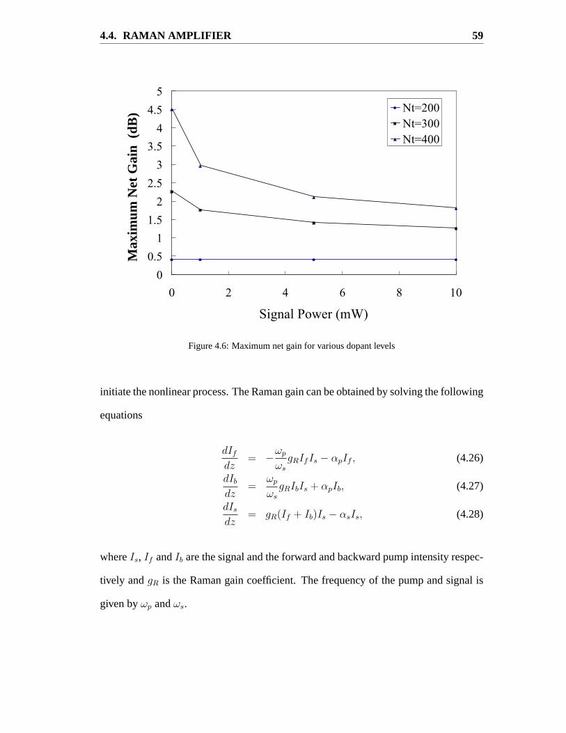
4.4. RAMAN AMPLIFIER 59
0
0.5
11.5
2
2.5
3
3.54
4.5
5
0 2 4 6 8 10
Signal Power (mW)
M
axim
um N
et G
ain
(dB
) Nt=200Nt=300Nt=400
Figure 4.6: Maximum net gain for various dopant levels
initiate the nonlinear process. The Raman gain can be obtained by solving the following
equations
dIf
dz= −ωp
ωs
gRIfIs − αpIf , (4.26)
dIb
dz=
ωp
ωs
gRIbIs + αpIb, (4.27)
dIs
dz= gR(If + Ib)Is − αsIs, (4.28)
whereIs, If andIb are the signal and the forward and backward pump intensity respec-
tively andgR is the Raman gain coefficient. The frequency of the pump and signal is
given byωp andωs.

4.4. RAMAN AMPLIFIER 60
4.4.1 Small Signal Analysis
We can solve Eqs. (4.26)-(4.28) analytically in the small-signal domain by assuming
that the pump intensity is dominated by fiber losses. The forward and backward pump
powers (note that we can convert intensity to power simply by usingP = I Aaeff )
are given similarly by Eqs. (4.15)–(4.16). The pump parameter that we derived in
Eq. (4.22) can also be applied to Raman amplification. Combining these equations, we
can write the Raman gain as
g(z) =gR
Aeff
[Pi exp(−αp z) +
C
Pi
exp(αp z)
]. (4.29)
Imposing the equal pump condition and fiber transparency (see Eq. (4.23)) yields the
following solution for the pump power needed
Po =αs αp LA Aeff
2 gR (1− exp(−αp LA)). (4.30)
4.4.2 Numerical Results
The small signal approximation is valid for most single-channel systems since SRS is
not a very efficient processes. For instance, even for average signals on the order of
mW, the pump absorption due to signal-gain depletion is only on the order of
gR Aeff Is = 10−16
[km
W
]10−3[W]
50× 10−18 [km2]≈ 0.01
dB
km, (4.31)
which is much smaller than typical fiber loss 0.2 dB/km. Nevertheless, as in the case of
d-EDFAs, the use of WDM technology greatly increases the total signal power that it

4.4. RAMAN AMPLIFIER 61
is often necessary to solve the equations exactly using numerical methods. The signal
power as well as well as the forward and backward are solved simultaneously to obtain
the gain
g(z) =gR
Aeff
[Pf (z) + Pb(z)] . (4.32)
Figure 4.7 shows numerical result of the pump power evolution and the gain of a 100
km section of fiber compensated through bi-directional pumped Raman gain for low
power signals. Note that the pump power needed is lower than a 100-km 200-ions/µm3
Figure 4.7: (Top) Numerical solution of forward (dotted line), backward (dashed line) and total pumppower (solid line) of Raman amplifier. (Bottom) Numerical solution of gain variations of Raman ampli-fier
d-EDFA but its net gain is larger in comparison.

4.5. AMPLIFIER PERFORMANCE 62
4.5 Amplifier Performance
We modify the generalized nonlinear Schrodinger equation, Eq. (3.1) to study the effect
of using distributed amplification as
∂U
∂ζ+
i
2sgn(β2)
∂2U
∂τ 2− iN2|U |2U =
(g(ζ)− α
2
)U − iτR
∂|U |2
∂τ, (4.33)
with τR is the SRS coefficient and with lumped amplitude gain given by
g(z) =(√
G− 1) N∑
n=1
δ(ζ − nζa). (4.34)
Distributed amplification using d-EDFA and Raman gain is included by solving for
the gain variation through Eq.(4.9) and Eq.(4.32) respectively. We used the split-
step Fourier-transform method [9] to compare soliton propagation for lumped and dis-
tributed amplification schemes.
We first demonstrate the advantages offered by distributed amplification for a 20
Gb/s system having 100-km pump-station spacing, uniform dispersion withβ2 = −0.5
ps2/km,γ = 3.36 W−1/km, τR = 3 fs andα = 0.23 dB/km at the operating wavelength
near 1.55 mm. The soliton width should be a fraction of the 50-ps bit slot. We choose
the input fieldA(0, t) =√
P0 sech(t/T0) with T0 = 5 ps (TFWHM = 8.8 ps). The
peak powerP0 corresponds toN = 1 for distributed amplification andN = 2.307
in the lumped amplification case as required in the average-soliton regime [2]. The
dispersion length is 50 km for such a system, and the amplifier spacing is chosen to be
100 km both cases.
Figure 4.8(a) shows soliton evolution for the case of lumped amplification. Since

4.5. AMPLIFIER PERFORMANCE 63
LA/LD = 2, the soliton develops significant dispersive waves after only 3 amplifiers
and is distorted significantly after 6 amplification stages. Such a system cannot transmit
Figure 4.8: Comparison of (a) lumped, (b) d-EDFA, and (c) Raman amplification schemes for the caseof a 20-Gb/s system designed with 100-km amplifier spacing.
the 20-Gb/s signal over more than 600 km. Figure 4.8(b) shows soliton evolution over
5000 km under identical operating conditions except for distributed amplification, with
no visible sign of degradation. The optimum dopant density is found to be only 200
ions/µm3 when the fiber is bidirectionally pumped using equal pump powers of 79 mW
at both ends. Figure 4.8(c) shows soliton evolution using Raman amplification. It uses
slightly less pump power, roughly 60 mW at each end although it also supports soliton
at the longer amplifier spacing; there were substantially more dispersive waves being
generated. A logarithmic plot of the pulse power (Figure 4.9) shows the contribution
of residual dispersive waves to remain below the10−4 level even after 5000 km for d-

4.5. AMPLIFIER PERFORMANCE 64
EDFA scheme while Raman amplification scheme has residual dispersion below10−2.
Figure 4.9: Level of dispersive wave using d-EDFA (solid line) and Raman amplification (dotted line)
The most important criterion for designing soliton systems with distributed ampli-
fication is to ensure that peak power varies as little as possible over each fiber span.
Figure 4.10 shows the variation of pump power and the net signal gain defined as
G(z) = exp(∫ z
0g(z) dz − αz) over one fiber span for the results shown in Figures
4.8(b). SinceG(z) < 0.4 dB, the soliton peak power varies less than 10%, compared
with more than 20-dB variation occurring for lumped amplification or the 2 dB varia-
tion for Raman amplification (Figure 4.7). In general, peak-power variations become
smaller as dopant density is reduced, but at the same time, required pump power in-
creases [40]. In practice, one must choose the dopant density as small as possible for a
given amount of pump power.

4.6. SUMMARY 65
4.6. SUMMARY 67
0 10 20 30 40 50 60 70 80 90 1000
20
40
60
80
Pow
er (
mW
)
Distance (km)
0 10 20 30 40 50 60 70 80 90 100
0
0.2
0.4
Distance (km)
Gai
n (d
B)
Figure 4.10: Pump power and gain variations of d-EDFA amplifier
Figure 4.10: (Top) Numerical solution of forward (dotted line), backward (dashed line) and total pumppower (solid line) of d-EDFA. (Bottom) Numerical solution of gain variations of d-EDFA
4.6 Summary
In this chapter, we set forth the models required to study distributed amplification using
lightly-doped erbium ions as well as using distributed Raman gain. We present analyt-
ical solutions for the design of these distributed amplifiers in the small-signal regime.
We also set forth the constrains needed to solve them numerically. In extending the
guiding-center soliton limitation of the amplifier spacing, we found that distributed
amplification can support solitons with amplifier spacing as large as2 LD. We also
demonstrated through numerical simulation of the nonlinear Schrodinger equation that

4.6. SUMMARY 66
distributed amplification can permit single-channel speeds of 20 Gb/s over transoceanic
distances while maintaining 100 km spacing between pumping stations.

67
Chapter 5
Dispersion-Management Systems
5.1 Introduction
The two biggest obstacles in the design of high-capacity lightwave transmission sys-
tems are fiber loss and chromatic dispersion. It has been shown earlier that the use of
distributed amplification can reduce the limitations of the guiding-center soliton ampli-
fier spacing (see Chapter 4). Another way of solving the dispersion problem is through
the use of dispersion management techniques. Thus far, the use of EDFAs in combi-
nation with dispersion management has produced commercial WDM systems having
single-channel bit rates of up to 10 Gb/s with practical amplifier spacings. However,
the increasing demand is pushing the industry toward systems with a capacity of a few
Tbit/s. Keeping the current single-channel bit rate of 10 Gb/s would require hundreds
of WDM channels in such systems. Increasing the single-channel bit rate to 40 and
80 Gb/s would reduce the number of multiplexed channels needed while simplifying
the network management [43] by reducing the number of components required.
Soliton communication system is a natural candidate for long-haul, ultra-high-bit-
rate lightwave transmission links, since the short pulse width required for high bit-rates
will also induced large nonlinearity that must be accounted for. Solitons can effectively

5.1. INTRODUCTION 68
use nonlinear SPM to dynamically balance GVD [2]. Most fiber-optic communication
system experiments employ the technique of lumped amplification and place fiber am-
plifiers periodically along the link to compensate for the fiber loss. However, lumped
amplification introduces large peak-power variations, which limit the amplifier spac-
ing, LA, to a fraction of the dispersion lengthLD [2]. At high bit rates (> 20 Gb/s),
the dispersion length can become quite small, making the use of lumped amplification
impractical. For example, a recent experiment demonstrating a 40 Gb/s soliton system
using dispersion management needed amplifier of 28 km [44]. Indeed, loss and gain
perturbations along the fiber link are the most serious obstacle in designing practical
soliton communication systems.
While many recent studies have considered novel dispersion maps and distributed
amplification schemes [45–48], and a few studies even have examined the added stabil-
ity of dispersion management with distributed amplification [46,47], a systematic study
on the system level performance which includes the effect of ASE and incorporates both
of these design features has not yet been performed. The performance of high-speed
single-channel systems (operating at 40 and 80 Gb/s) with large amplifier spacings (100
km and 40 km, respectively) is examined in this thesis using several different hybrid
amplification schemes. Two-step as well as dense dispersion-management configura-
tions are used in conjunction with a variety of lumped and distributed amplification
schemes. Specifically, the performance of lightwave systems using lumped amplifiers,
hybrid amplifiers (backward-pumped Raman with EDFA), bidirectionally pumped Ra-
man amplifiers (d-Raman), and distributed EDFA are compared.

5.2. DISPERSION MANAGED SOLITON 69
5.2 Dispersion Managed Soliton
Dispersion Management uses spatially varying dispersion along the fiber to combat the
effect of GVD. There are two basic techniques which consist of either using dispersion-
decreasing fibers [9,49,50] or periodic dispersion maps. A dispersion decreasing fiber
matches the dispersion of the fiber to the loss profile of the fiber. Such fibers are dif-
ficult to make and are not yet available commercially. The most popular technique of
dispersion management by far is the use of a periodic dispersion map to compensate
for GVD.
Substantial work has been done on the stability and the conditions of dispersion-
managed solitons using a variety of techniques [51–58]. By far, the most commonly
used technique has been the use of variational analysis [20,52,57]. The theoretical
framework using variational analysis to calculate the amount of prechirping and launch-
ing power needed for stable pulse propagation is presented below.
5.2.1 Variational Analysis
Variational analysis is used to develop an approximate solution in a periodic disper-
sion map. It has been shown in Chapter 3 that prechirping is necessary for additional
soliton control in establishing soliton periodicity. We also have seen that the creation
of solitons necessities a careful balance of nonlinearity and dispersion, so calculating
the optimal launching power is also critical. Studies have shown that a detuning of the
input soliton energy from its optimal value can generate dispersive-wave emission that
can contribute to long-range soliton-soliton interactions [59,60].
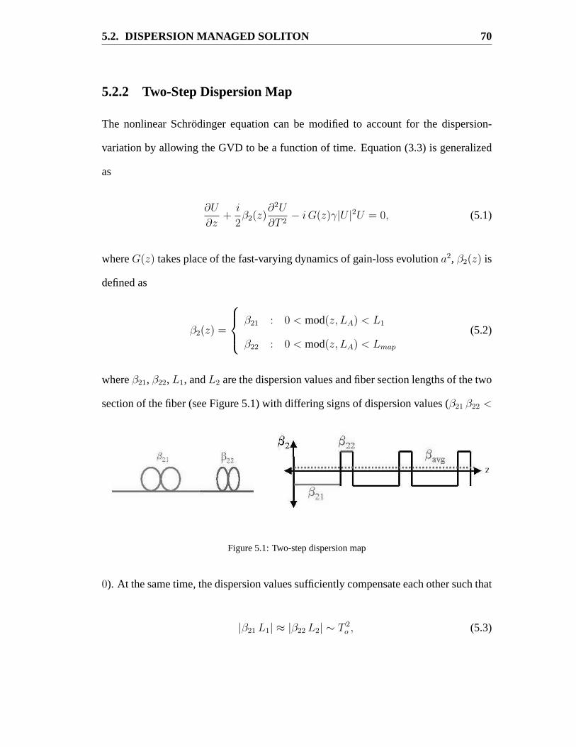
5.2. DISPERSION MANAGED SOLITON 70
5.2.2 Two-Step Dispersion Map
The nonlinear Schrodinger equation can be modified to account for the dispersion-
variation by allowing the GVD to be a function of time. Equation (3.3) is generalized
as
∂U
∂z+
i
2β2(z)
∂2U
∂T 2− i G(z)γ|U |2U = 0, (5.1)
whereG(z) takes place of the fast-varying dynamics of gain-loss evolutiona2, β2(z) is
defined as
β2(z) =
β21 : 0 < mod(z, LA) < L1
β22 : 0 < mod(z, LA) < Lmap
(5.2)
whereβ21, β22, L1, andL2 are the dispersion values and fiber section lengths of the two
section of the fiber (see Figure 5.1) with differing signs of dispersion values (β21 β22 <
z
Figure 5.1: Two-step dispersion map
0). At the same time, the dispersion values sufficiently compensate each other such that
|β21 L1| ≈ |β22 L2| ∼ T 2o , (5.3)

5.2. DISPERSION MANAGED SOLITON 71
whereτo is the pulse width.
It is convenient to renormalize the system with respect to dispersion mapLmap,
normalized soliton energyUo, and pulse [52],
ξ =z
Lmap
, u =U
Uo
, ς =T√
L1 L2 |β21−β22|Lmap
. (5.4)
This normalization allows us to rewrite the equation as follow
iuξ −1
2β2(ξ) uςς + ε
[1
2β2uςς + G(ξ)u|u|2
]= 0 (5.5)
whereε and the average dispersion,β2 are defined as
ε = Lmap γ |Uo|2, (5.6)
β2 =β21L1 + β22L2
L1 L2|β21 − β22| |Uo|2. (5.7)
Following the analysis set forth in 2.5, we will replace the soliton ansatz in
Eq. (2.63) with a Gaussian ansatz of the form
uo =A√(
1 + 2i(
∆ς2o
)) exp
(iφ− iς2
ς2o + 2i∆
). (5.8)
whereA is the amplitude,ςo is the initial normalized width,∆ is the normalized chirp
parameter, andφ is the phase. The corresponding pulse parameter evolution is then

5.2. DISPERSION MANAGED SOLITON 72
[52]
A2 ςo = E = constant, (5.9)
dς
dξ=
√2ε G(ξ) E ςo∆(ξ)
W 3(ξ), (5.10)
d∆
dξ= εβ2 +
ε G(ξ) E [4∆2(ξ)− ς4o ]
2√
2W 3(ξ), (5.11)
with varying width defined as
W (ξ) =4∆2 − ς4
o
ς0. (5.12)
As in chapter 3, the periodicity condition can be imposed on the system as
ςo(ξ) = ς(ξ + 1), ∆o(ξ) = ∆o(ξ + 1) (5.13)
with the new normalized width and chirp (also note that the length is now normalized
to Lmap). This is done by integration Eq. (5.10) and (5.11) from 0 to 1 and requiring
them to be 0. With a simple change of variables using
ξ =
L1(s + 12) : 0 < ξ < L1
L1 + L2
(12− s)
: L1 < ξ < 1(5.14)

5.2. DISPERSION MANAGED SOLITON 73
the periodicity boundary condition yields the following constrains [52]:
∫ 0.5
−0.5
[s + ∆o + 1
2
]g(s) ds[
ς4o + 4
(s + ∆o + 1
2
)2] 32
= 0, (5.15)
β2 =
√2A2ς4
o
4
∫ 0.5
−0.5
[4(s + ∆o + 1
2
)2 − ς4o
]g(s) ds[
ς4o + 4
(s + ∆o + 1
2
)] 32
, (5.16)
where
g(s) = L1 G
(L1(s +
1
2)
)+ L2 G
(L1 + L2(
1
2− s)
). (5.17)
The normalized chirp∆o parameter is obtained by solving Eq. (5.15) and the normal-
ized launching powerA2 is obtained by solving Eq. (5.16). The gain characteristics
of the different amplification schemes can be easily incorporated through modifying
Eq. (5.17).
5.2.3 Dense Dispersion Management
The strength of a DM map is defined as
Smap =|β21 L1 − β22 L2|
τ 2FWHM
, (5.18)
whereτFWHM is the full width half maximum of the pulse and is related to the char-
acterized pulse widthτo by τFWHM ≈ 1.665τo for Gaussian pulses. This parameter
characterizes the amount of perturbation a dispersion-varying medium has on the pulse.
Typically, DM solitons are stable whenSmap < 3 [52]. But as the single-channel bit
rate is increased the pulse width decreases. This can dramatically increase the map

5.2. DISPERSION MANAGED SOLITON 74
strength, especially if the map period,Lmap = L1 + L2, (which until now is equivalent
to the amplifier spacing) is kept relatively large. This will severely limit the amplifier
spacing of high-bit rate systems. Dense DM map systems overcome this by allowing
the amplifier spacing to contain multiple map periods (LA = M Lmap), whereM is an
integer. This allows the use of relatively tamed maps for pulse propagation at high bit
rates while maintaining a large amplifier spacing (see Figure 5.2).
Figure 5.2: (Top) Two-step dispersion map. (Bottom) Dense dispersion map
The formula derived in the previous section is still valid in calculating the launching
condition for dense DM map systems with only the gain needs to be modified. Equation
(5.17) can be generalized as
g(s) =M∑
m=0
exp
(−m α Lmap
2
)[L1 G
(L1(s +
1
2)
)+ L2 G
(L1 + L2(
1
2− s)
)].
(5.19)

5.3. SYSTEM PERFORMANCE 75
5.3 System Performance
System performance can be gauged through observation of the received eye diagram.
The eye diagram is a superposition of the pulse train in various combinations and gives
in general an excellent indicator on the system performance. The more“open” the eye
appears, the better the decision circuits can differentiate the “1” from the “0” bit and
therefore, the less likely it is to make an error. It is beneficial to have a figure of merit to
quantify the eye opening of the eye diagram for system performance characterization.
The system performance is quantified through the use of the Q factor, which approxi-
mates the bit-error rate (BER) and is defined as (see Appendix B)
Q =I1 − I0
σ1 + σ0
(5.20)
whereI1, I0, σ1 andσ0 are the intensity and the standard deviation of the received ”1”
and ”0” of the bit pattern. In order to accurately calculate the Q, it is necessary to
include the noise in the system.
5.3.1 Amplifier Noise
Amplified spontaneous emission (ASE) noise comes from the spontaneous emission
amplified through cascade of optical amplifiers. The amount of ASE generated per a
given bandwidth is given by
PASE = 2 nsp h ν ∆ν (G− 1) (5.21)

5.3. SYSTEM PERFORMANCE 76
wherensp is the spontaneous emission factor,h is the Planck’s constant,ν is the fre-
quency, and∆ν is the bandwidth. The spontaneous emission factor can be written as a
ratio of the ground and excited-level populations
nsp =NT −N1
NT − 2N1
, (5.22)
which describes the amount of inversion of the system. Noise figure NF is often used
when characterizing the noise performance of a system and it is defined asNF =
10 log(2 nsp). For fully-inverted amplifier,N1 = 0, thensp is 1. Note that since the
d-EDFA consists of long length of fiber, the NF changes as a function of distance [via.
N1(z)].
5.3.2 Numerical Results
In this section, 40 and 80 Gb/s systems using different amplification schemes and dis-
persion maps are examined using the Q factor to compare system performance. For a
bit rate of 40 Gb/s, it is necessary to use a pulse width of only 2.5 ps (TFWHM = 4.4
ps). Using the same design parameters as for the 20-Gb/s distributed amplification sys-
tem in Chapter 4, the dispersion length is calculated to be only 12.5 km. To account
for soliton interaction, a 64-bit pseudorandom sequence is used in numerical simula-
tions. The two-bit-wide optical “eye diagram” (unfiltered) displayed in Figure 5.3(a)
shows the combined effects of Raman-induced soliton self frequency shift (SSFS) and
soliton interaction on the pulse train at a distance of 1000 km using lumped amplifica-
tion excluding ASE. Clearly such a system will perform poorly in practice. We have
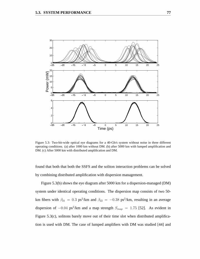
5.3. SYSTEM PERFORMANCE 77
5.4. SUMMARY 81
0 5 10 15 20 250
10
20
30
0 5 10 15 20 250
5
10
15
20
Pow
er (
mW
)
0 5 10 15 20 250
2
4
6
Time (ps)
Figure 5.3: Two-bit-wide eye diagrams for a 40-Gb/s system in three different operating conditions. (a)after 1000 km without DM. (b) after 5000 km with lumped amplification and DM. (c) After 5000 kmwith distributed amplification and DM.
Figure 5.3: Two-bit-wide optical eye diagrams for a 40-Gb/s system without noise in three differentoperating conditions. (a) after 1000 km without DM. (b) after 5000 km with lumped amplification andDM. (c) After 5000 km with distributed amplification and DM.
found that both that both the SSFS and the soliton interaction problems can be solved
by combining distributed amplification with dispersion management.
Figure 5.3(b) shows the eye diagram after 5000 km for a dispersion-managed (DM)
system under identical operating conditions. The dispersion map consists of two 50-
km fibers withβ21 = 0.3 ps2/km andβ22 = −0.38 ps2/km, resulting in an average
dispersion of−0.04 ps2/km and a map strengthSmap = 1.75 [52]. As evident in
Figure 5.3(c), solitons barely move out of their time slot when distributed amplifica-
tion is used with DM. The case of lumped amplifiers with DM was studied [44] and

5.3. SYSTEM PERFORMANCE 78
it was found that both SSFS and soliton interaction are reduced in this case as well
(Figure 5.3(b)) although system performance is better in the case of distributed ampli-
fication (Figure 5.3(c)).
Noise is included in the system by using a noise figure of 4.5 dB for EDFAs and 3
dB for Raman amplifiers. The launch power and initial chirp are calculated using the
results of a variational analysis for dispersion-managed solitons. The distributed gain
(for both d-EDFA and Raman amplifiers) is obtained numerically taking into account
gain saturation and pump depletion. The results of the system simulation for different
amplification schemes are shown in Fig. 5.4. where system performance as measured
by Q is plotted vs. propagation distance. The maximum transmission can be deduced
by noting thatQ = 6 corresponds to BER of about10−9.
Figure 5.4 shows clearly the advantage of distributed amplification for high-speed
lightwave systems. When lumped EDFAs are used, the transmission distance is limited
to below 500 km, but increases to 3400 km for d-EDFA. Use of Raman amplification
also improves the performance, although not as much as d-EDFA. The reason for this
is that the design of a d-EDFA can be optimized by adjusting the dopant concentration.
A Raman amplifier does not have this additional degree of freedom. The net gain over
the 100-km amplifier span is only 0.5 dB for optimized d-EDFA but it increases to 6 dB
for a distributed Raman amplifier and to over 15 dB for a hybrid amplification scheme
(see Figure 5.5).
As the single-channel bit rate increases beyond 40 Gb/s, a reduced pulse width and
a practical amplifier spacing combine to create a dispersion map that is too strong for
stable propagation of solitons. A solution is provided by the technique of dense dis-
persion management [48] for which amplifier spacing is chosen to be a multiple of

5.3. SYSTEM PERFORMANCE 79
Q = 6
Figure 5.4: System performance of a 40-Gb/s DM soliton system using different amplification schemes.
the map period, which can be reduced to below 10 km. 2.93-ps pulses are launched
into a dispersion map consisting of 2.231-km sections withβ21 = 3.2 ps2/km and
β22 = −3.2 ps2/km, resulting in an average dispersion of -0.013 ps2/km and a map
strength of 1.65. The amplifier spacing of 40 km corresponds to 9 map periods. Figure
5.6 shows the performance of such an 80-Gb/s, multiple-cell soliton system for vari-
ous amplification schemes. The results show again that the transmission distance can
be increased using distributed amplification. Although one might expect the system
performance (Q) to be a strictly monotonically decreasing function of distance, how-
ever, the system operates with two distinct dynamic time scales. There is a fast time
scale that revealed the rapid oscillation of the pulse width and power due to periodic

5.3. SYSTEM PERFORMANCE 80
5.4. SUMMARY 83
Figure 5.5: Net gain vs. distance for (a) hybrid, (b) distributed Raman, and (c) distributed-erbiumamplification schemes.
Figure 5.5: Net gain vs. distance for hybrid (top), distributed Raman (middle) , and distributed-erbiumamplification schemes (bottom).
variations of the dispersion and amplification, and a second slow time scale that results
from the combined effects of nonlinearity, residual dispersion, and pulse prechirping
[61]. Nevertheless, it is clear from Figure 5.7, which plots the pulse evolution of a pair
of solitons (corresponding to a pattern of 0 1 1 0) as it propagates through the system,
that the advantage of the distributed amplification systems is to significantly reduce the
effect of pulse to pulse interactions.

5.4. SUMMARY 81
Q = 6
Figure 5.6: System performance of a 80-Gb/s DM soliton system using different amplification schemes.
5.4 Summary
Distributed amplification can increase the total transmission distance of ultra-high-bit-
rate systems employing different dispersion maps. The improvement depends not only
on the amplification scheme but also on details of the dispersion map. For systems lim-
ited by amplified spontaneous emission because of a relatively long amplifier spacing,
the use of erbium doping provides best performance. Simulation results of 40 Gb/s sys-
tems using two-step dispersion map and 100 km amplifier spacing showed an increase
of up to a factor of 7 in the maximum distance allowed by using d-EDFAs verus ED-
FAs. For systems limited by the map strength, the benefit of distributed amplification
(Raman or erbium-doping) comes from the smaller net gain and a lower effective noise

5.4. SUMMARY 82
Figure 5.7: Pulse-to-pulse interaction for a 80-Gb/s soliton system using (a) EDFA, (b) hybrid, (c) dis-tributed Raman, and (d) distributed erbium amplification schemes
figure. Simulation results of 80 Gb/s systems using dense dispersion map and 40 km
amplifier spacing showed an increase of up to a factor of 2 in the maximum distance
allowed by using d-EDFAs verus EDFAs.

83
Chapter 6
Fiber Lasers
6.1 Introduction
Ideally, we would liked to compare the results of our numerical simulations with ex-
perimental transmission systems. Unfortunately, such systems are expensive and hard
to come by. In an effort to establish a transmission system from the ground up, we have
focused much of our experimental efforts to the understanding and characterization of
fiber lasers, which can be used as transmitters, the first building block of a fiber-optic
communication systems.
6.2 Experimental Setup
The ring-cavity of our fiber laser (see Fig. 6.1) consists of 7.2 m of erbium-doped fiber
and 11.1 m of standard fiber, resulting in a total cavity length of18.3 m [see Figure 6.1]
[62]. A 980-nm pump laser diode (LD) (Lasertron QLM9S470) injects light through
a 980/1550-nm WDM coupler; it couples about 95% of the pump light into the cavity.
The output coupler transmits approximately 10% of the bidirectional circulating powers

6.2. EXPERIMENTAL SETUP 84
5.6. SUMMARY 57
980 pump LDPhotodiode
Photodiode
Erbium doped fiber
980/1550 WDM
95/5 coupler
1550nm
90/10 coupler
Monitor
Co-propagating
Counter-propagating
Figure 5.1: Experimental Configuration of Fiber Laser
Figure 6.1: Experimental configuration of the fiber laser
per round trip. Each end of the output coupler is connected to a large-area germanium
photoreceiver (New Focus Model 2033).
6.2.1 Output Power
We first measured the output power from the fiber laser through the monitor (Pmonitor),
and the sum of the co-propagating and counter-propagating ports (Ptot) as a function
of the pump current. As is evident from Figure 6.2, the threshold for the 980-nm pump
LD (which is measured through the monitor port) is 20 mA. The power emitted by the
fiber laser in each counter propagating direction is observed through the output port of
the 90/10 1550 nm coupler. The threshold for the fiber laser is measured to be 30 mA,
which translate roughly to 5 mW of pump power at 980 nm. The slope efficient is about
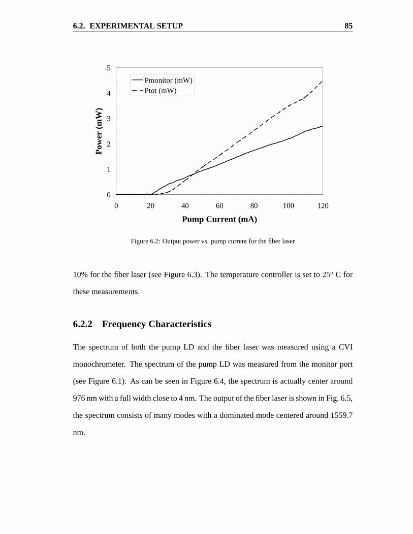
6.2. EXPERIMENTAL SETUP 85
0
1
2
3
4
5
0 20 40 60 80 100 120
Pump Current (mA)
Pow
er (m
W)
Pmonitor (mW)Ptot (mW)
Figure 6.2: Output power vs. pump current for the fiber laser
10% for the fiber laser (see Figure 6.3). The temperature controller is set to25o C for
these measurements.
6.2.2 Frequency Characteristics
The spectrum of both the pump LD and the fiber laser was measured using a CVI
monochrometer. The spectrum of the pump LD was measured from the monitor port
(see Figure 6.1). As can be seen in Figure 6.4, the spectrum is actually center around
976 nm with a full width close to 4 nm. The output of the fiber laser is shown in Fig. 6.5,
the spectrum consists of many modes with a dominated mode centered around 1559.7
nm.

6.3. MODE-PARTITION NOISE 86
y = 0.0987x - 0.5
0
1
2
3
4
5
0 10 20 30 40 50
Pump Power (mW)
Out
put P
ower
(mW
)
Figure 6.3: Output power vs. pump power for the fiber laser
6.3 Mode-Partition Noise
Mode-partition noise has been observed in a variety of lasers including semiconductor
lasers [63,64], gas lasers [65], and dye lasers [66]. In semiconductor lasers, mode-
partition noise arises from competition among multiple longitudinal modes. Mode-
partition noise can also occur when cavity design forces co and counter-propagating
modes to compete for the same gain. In particular, bidirectional-ring dye lasers have
been found to exhibit random on-off switching between the two counter-propagating
modes of the cavity such that whenever one mode turns on, the other turns off com-
pletely [66]. This phenomenon is attributed to the strong mode coupling that can occur
in a homogeneously-broadened gain medium [67]. Fiber lasers are made using silica
fibers whose core is doped with rare-earth ions, together with other codopants such as
aluminum and germanium. Depending on the proportion of codopants, the gain spec-

6.3. MODE-PARTITION NOISE 87
0
0.01
0.02
0.03
0.04
0.05
0.06
0.07
970 972 974 976 978 980
Wavelength (nm)
Pow
er
Figure 6.4: Spectrum of the pump output
trum of fiber lasers can be dominated by homogeneous or inhomogeneous broadening
[68]. In this section, we present the experimental evidence of mode-partition noise in
fiber lasers. We have also developed a theoretical model, based on the Langevin rate
equations, whose predictions agree well with our experimental results.
6.3.1 Experimental Observation
Temporal evolution of the photoreceiver signals is monitored using an oscilloscope.
Since we do not use an intracavity isolator, the laser emits light in both the clockwise
and counter-clockwise directions. Figure 6.6 shows the output powers for the two di-
rections when the laser is pumped 2.6 times above its threshold. The two modes are
almost perfectly anti-correlated; an increase in the power of the one mode corresponds

6.3. MODE-PARTITION NOISE 88
0
0.002
0.004
0.006
0.008
0.01
0.012
0.014
1555 1557 1559 1561 1563 1565
Wavelength (nm)
Pow
er
Figure 6.5: Spectrum of the fiber laser output
to a decrease in the other. The sum of the powers remains nearly constant, except for
small fluctuations occurring at the relaxation oscillation frequency (≈ 29 kHz). The
individual powers on the other hand, fluctuate on a rather slow time scale (∼ 0.1 s).
These fluctuations are due to mode-partition noise induced by cross-gain saturation.
This interpretation is confirmed by the theoretical model presented next. Figure 6.6 is
snap shot of the temporal evolution of the signal on a 20 second time interval.
6.3.2 Mode-Partition Noise Theory
We use the standard three-level rate-equation model but simplify it by assuming rapid
transfer of the pumped population to the excited state. The resulting rate equations with

6.3. MODE-PARTITION NOISE 89
1
1.5
2
2.5
0 5 10 15 20Time (s)
Po
wer
(m
W)
Figure 6.6: Output power of fiber laser for clockwise mode (middle), counter-clockwise mode (bottom),and sum of the two modes (top)
added Langevin noise terms can be written as [69]
P1 = (BN − γ)P1 + Rsp + F1(t), (6.1)
P2 = (BN − γ)P2 + Rsp + F2(t), (6.2)
N = Wp(NT −N)− 2(P1 + P2)BN − (N + NT )/T1, (6.3)
whereP1 andP2 are the number of photons in the co- and counter-propagating modes,
respectively, andN represents the population-inversion level. The cavity-decay rateγ
is related to the photon lifetimeτp asγ = 1/τp. The rate of spontaneous emission is
taken to beRsp = nspBN , wherensp is the inversion parameter, andB is related to the
rate of stimulated emission. In Eq. (6.3),Wp is the pump rate,NT is the total number

6.3. MODE-PARTITION NOISE 90
Table 6.1: Parameters used in simulation of fiber laser dynamics
Parameter Symbol ValueAverage photons in the clockwise mode P1 4.056× 10⁹
Average photons in the counter-clockwise modeP2 3.314× 10⁹
Population inversion density N 4× 10²³m−3
Total dopant density NT 1× 1025m−3
Rate of cavity decay γ 4.14× 10⁶s−1
Population relaxation time T1 1× 10⁻²sPump photon rate WP 390s−1
Effective active volume Va 2.256× 10⁻¹¹m3
Rate of stimulated emission B 4.588× 10⁻⁷s−1
of dopants, andT1 is the fluorescence time. The coupling betweenP1 andP2 is solely
due to cross-gain saturation resulting from gain sharing.
The Langevin noise sourcesF1(t) andF2(t) are responsible for fluctuations inP1
andP2, respectively. They vanish on average (< Fi(t) >= 0). Assuming noise to be
Markoffian (white noise), we use [69]
< Fi(t)Fj(t′) >= 2Dijδ(t− t′), (6.4)
wherei, j = 1, 2. The diffusion coefficient are related to the rate of spontaneous emis-
sion as
D11 = RspP1, D22 = RspP2, D12 = 0, (6.5)
whereP1 andP2 are the average steady-state values.
The stochastic rate equations Eq. (6.1)–(6.3) are solved numerically using param-
eter values appropriate to our fiber laser (a noise figure of 3.4 dB corresponding to

6.4. SUMMARY 91
nsp = 1.1 is assumed). Figure 6.7 shows a 5 second section of the time series simulated
numerically. Comparing Fig. 6.6 and 6.7, we see that our model reproduces all qual-
itative features of the mode-partition noise observed experimentally. This agreement
April 28, 2000 ZML: Ditech
Theory and Predictions
Figure 6.7: Numerical simulation of output powers in clockwise (top curve) and counter-clockwise (bot-tom curve) directions.
confirms that the anticorrelation seen in Fig. 6.6 has its origin in cross-gain saturation.
6.4 Summary
We have built and characterized an erbium-doped fiber laser pumped by a 980 nm LD.
We observed a threshold of 20 mA for the pump LD and 30 mA for the fiber laser.

6.4. SUMMARY 92
With respect to the pump light, the lasing threshold was measured to be 5 mW. The
slope efficiency of the fiber laser was found to be 10%. The spectrum of the fiber laser
was measured to be centered at 1559.7 nm with a linewidth of approximately 2 nm.
We have also experimentally observed mode-partition noise in a fiber laser. We have
developed a rate-equation model that is capable of reproducing the experimentally ob-
served behavior. We did not observe complete on-off switching similar to that observed
in dye lasers [66]. We believe that the inhomogeneous broadening of the gain spectrum
in our fiber laser leads to weak mode coupling. It is well known that codopants such as
aluminum can make the gain spectrum nearly homogeneously broadened. Such fiber
lasers may exhibit complete on-off switching.

93
Chapter 7
Conclusions
7.1 Overview
This thesis developed several techniques and concepts that will help shape the next
generation of high-capacity fiber-optic communication systems. The principal target
has been to increase the amplifier spacing through various techniques in present and
future systems. In this chapter, we will expand and elaborate on the three main research
areas covered in this thesis: design of constant dispersion system, design of dispersion
management systems, and fiber laser dynamics. In each section, we will summarize
our findings and provide additional insights for future research.
7.2 Constant-Dispersion Fibers
For a constant-dispersion system, soliton evolution through a lossy medium can be
described by the guiding-center soliton theory. This allows stable propagation of soliton
pulses provided that the fiber loss is compensated and the amplifier spacing is a fraction
of the the dispersion length. Extending the amplifier spacing can be achieved in two
ways: providing an additional degree of freedom in the guiding center soliton theory

7.2. CONSTANT-DISPERSION FIBERS 94
to relax the amplifier-spacing constraint or to replace the large perturbation of lumped
amplification by distributed amplification.
In Chapter 3, we used the variational analysis to solve the periodicity condition for
pulse propagation in a lumped-amplification system by allowing both the pulse width
and the chirp to change over the amplifier spacing. We were able to recover the input
power condition as prescribed by the guiding-center soliton theory in the small ampli-
fier spacing regime (LA � LD) while, at the same time, predict the additional power
and the initial chirp needed for the large amplifier regime (LA ≥ LD). Our numer-
ical results show a much greater stability for systems operating at amplifier spacing
exceeding those valid for the guiding-center solitons.
Amplifier spacing can also be extended by noting that the amplifier spacing con-
strain is a result of the large perturbation caused by the use of lumped amplifiers which
give a large kick to the system within a very small distance (the longer the amplifier
spacing, the larger the gain needed to compensate for fiber loss). In Chapter 4, we have
seen that the use of distributed amplification can make the fiber appear transparent to
the optical pulses. We use distributed erbium-doped fiber amplifiers as well as Raman
gain to design distributed-amplification systems. The optimal pump configuration is bi-
directional pumping as it allows a more uniform gain distribution for the system. Unlike
the distributed Raman amplifiers, d-EDFA has an additional degree of freedom which
allows the amplifier to be designed with minimal gain excursion. The penalty to pay
for the low gain excursion is the higher pump power needed for d-EDFA. Although at
high dopant concentration, less pump power is needed for loss compensation since the
pump power does not need to penetrate deep into the fiber and work as hard (because
the high dopant is able to provide a large gain in a short span close to the pump). Of

7.2. CONSTANT-DISPERSION FIBERS 95
course, there is a limit — at too low a dopant density, no amount of pump power is able
to compensate for the fiber loss at the signal and the pump wavelengths. For a 100-km
distributed amplifier, gain excursion using a d-EDFA only experienced 0.4 dB by using
a dopant density of 200 ions/µm3 while distributed Raman amplifiers experienced 2-dB
gain excursion (as compared to lumped amplifiers of 20 dB gain excursion). The pump
power at each direction needed for d-EDFA was nearly 80 mW, slightly larger than the
pump power needed for distributed Raman (60 mW). Backward-pumped Raman gain
has already attracted considerable attention for current system designers to achieve ex-
tra system margin; it will be only a matter of time before system complexity can only
be solved through distributed-amplification solutions.
Our study has shown the advantage of prechirping and distributed amplification
in extending the amplifier spacing in high-bit-rate single-channel constant-dispersion
soliton communication systems. On a practical note, prescribing precise chirp at the
launching of a pulse is not a trivial issue, although chirp can be provided by simply
propagating the pulse through a fixed length of fiber, because measurements of fiber
length or GVD in the field are not precise enough. Further studies on the sensitivity of
the initial input parameters vs. the system stability will provide critical information on
the feasibility of this technique. The capacity of the system can be greatly increased
if WDM technology is employed. Further investigation is needed to study the effect
of prechirping and distributed amplification in a WDM system. Our analysis has al-
ready shown that the small-signal analytical solution is insufficient to describe the gain
distribution; the presence of multiple channels in a WDM system will surely present
similar challenges since the sum of the channel powers can easily exceed 40 mW. Fur-
thermore, the presence of constant, undiminished power at each of the channels along

7.3. DISPERSION-MANAGEMENT TECHNIQUE 96
the transmission line can further increase the nonlinear penalties such as cross-phase
modulation (XPM) and four-wave mixing (FWM) [9].
7.3 Dispersion-Management Technique
In Chapter 5, we presented the technique of dispersion management in soliton trans-
missions. The two-step dispersion map allows compensation of chromatic dispersion
through the use of fibers with normal and anomalous GVD. For ultra-high-bit-rate sys-
tems, it was necessary to use multiple dispersion maps within an amplifier spacing to
keep the map strength low enough for stable pulse propagation. We have also gath-
ered current amplifier technologies as well as developed future technologies such as
d-EDFA and bi-directional pumped Raman amplifiers in conjunction with dispersion
management in an effort to study the advantages of using each kind of amplifier.
Since distributed amplifiers offer better noise performance for systems limited by
noise, distributed amplification was able to outperform other schemes (lumped amplifi-
cation and hybrid amplification) by being able to transmit over seven times the distance
for a 40 Gb/s system. However, for systems limited by dispersion map, distributed
amplification was not able to offer as much advantage. Nonetheless, a lower gain ex-
cursion, and therefore a smaller soliton-soliton interaction effect, can also improve the
system performance of distributed amplifiers over lumped amplifiers, by roughly in-
creasing the transmission distance by a factor of 3 times over a 80 Gb/s system. The
effect of collision-induced timing jitter in dispersion-managed systems has been shown
to degrade the system performance in WDM systems. This has been attributed to the
asymmetric collisions at the amplifier nodes; it would be of extreme interest to study
how this effect changes with distributed-amplification schemes. Dispersion-managed

7.4. FIBER-LASER DYNAMICS 97
solitons have also been shown to be able to reduce the Gordon-Haus timing jitter be-
cause of the ability of the dispersion to create a potential trapping for the soliton pulses.
Further studies of this effect in conjunction with distributed amplification will also be
fruitful.
7.4 Fiber-Laser Dynamics
In Chapter 6, we characterized the operation of a fiber laser in an ongoing effort to
build a transmitter for a fiber-optic transmission system. The threshold as well as the
spectrum properties of the pump LD and the fiber laser was measured. We also experi-
mentally demonstrated mode-partition noise in a fiber laser. The theoretical model was
successful in duplicating the phenomenon. It is well known that the complete on-off
switching that has been reported for dye lasers is an effect of the homogeneous na-
ture of the gain medium; the lack of this similar phenomenon in the fiber laser can be
attributed to the inhomogeneous broadening of the gain spectrum. Since fibers with
codopants such as aluminum has been known to be able to make the fiber nearly ho-
mogeneous, it would be worthwhile to test the above hypothesis by duplicating the
experiment with aluminum-doped fiber lasers.
7.5 Summary
As evident in the previous chapters, this thesis seeks to explore the issues in expanding
amplifier spacing for a wide range of soliton-communication systems while maintaining
or surpassing the system performance. We can summarize the contribution of this work
to the development of soliton-communication system as follows:

7.5. SUMMARY 98
• Expanded on Guiding-center soliton theory by prechirping the pulse, which pro-
vides an additional degree of freedom for satisfying the periodicity conditions.
• Demonstrated a new regime of operation beyond that of Guiding-center solitons
whereLD ≥ LA.
• Predicted the ability of distributed amplification to extend the performance be-
yond the Guiding-center soliton whereLD ≥ LA.
• Predicted an improvement in the system performance (through greater transmis-
sion distance) with the use of distributed amplification in a two-step dispersion
managed system because of a better noise figure.
• Predicted an improvement in the system performance (through greater transmis-
sion distance) with the use of distributed amplification in a dense dispersion man-
aged system because of a smaller gain excursion.
• Constructed and characterized the operation threshold and the spectrum proper-
ties of an erbium-doped fiber laser.
• Experimentally demonstrated and theoretically verified the effect of mode-
partition noise in fiber lasers.
These advances have significantly advanced the theory and design of high-capacity
soliton transport systems, especially in the realm of distributed amplification.

99
Bibliography
[1] Technical report, Merrill Lynch: Global Fundamental Equity Research Depart-ment (unpublished).
[2] G. P. Agrawal,Fiber-Optic Communication Systems, 2 ed. (John Wiley & Sons,Inc., New York, 1991).
[3] T. Li, “The impact of optical amplifiers on long-distance lightwave telecommuni-cations,” Proc. IEEE.81, 1568 (1993).
[4] T. N. Nielsen et al., “3.28-Tb/s (82x40 Gb/s) transmission over 3x1000 kmnonzero-dispersion fiber using dual C- and L-band hybrid Raman/erbium-dopedinline amplifiers,” Opt. Fiber Confer.Postdeadline Papaers, PD23 (2000).
[5] T. Ito, K. Fukuchi, Y. Inada, T. Tsuzaki, M. Harumoto, and M. Kakui, “3.2 Tb/s –1500 km WDM transmission experiment using 64 nm hybrid repeater amplifiers,”Opt. Fiber Confer.Postdealing Papers, PD24 (2000).
[6] A. K. Srivastavaet al., “Ultra-dense terabit capacity WDM transmission in L-band,” Opt. Fiber Confer.Postdealine Paper, PD27 (2000).
[7] T. Terahara, T. Hoshida, J. Kumasako, and H. Onaka, “128x10.66 Gbit/s transmis-sion over 840-km standard SMF with 140-km optical repeater spacing (30.4-dBloss) employing dual-band distributed Raman amplification,” Opt. Fiber Confer.Postdeadline Papaers, PD28 (2000).
[8] N. Zabusky and M. D. Kruskal, “Interaction of solitons in collisionless plasma andthe recurrence of initial states,” Phys. Rev. Lett.15, 240 (1965).
[9] G. P. Agrawal,Nonlinear Fiber Optics, 3 ed. (Academic Press, San Diego, 2001).
[10] A. Hasegawa and F. Tappert, “Transmission of stationary nonlinear optical pulsesin dispersive dielectric fibers,” Appl. Phys. Lett.23, 142 (1973).
[11] L. Mollenauer, R. H. Stolen, and J. P. Gordan, “Experimental observation of pi-

BIBLIOGRAPHY 100
cosecond pulse narrowing and solitons in optical fibers,” Phys. Rev. Lett.45, 1095(1980).
[12] A. Hasegawa, “Amplification and reshaping of optical solitons in a glass fiber IV:Use of the stimulated raman process,” Opt. Lett.8, 650 (1983).
[13] L. F. Mollenauer, R. H. Stolen, and M. N. Islam, “Experimental demonstration ofsoliton propagation in long fibers: Loss compensated by raman gain,” Opt. Lett.10, 229 (1985).
[14] L. F. Mollenauer, J. P. Gordan, and M. N. Islam, “Soliton propagation in longfibers with periodically compensated loss,” IEEE J. Quantum Electron.22, 157(1986).
[15] L. F. Mollenauer and K. Smith, “Demostration of soliton transmission over morethan 4000 km in fiber with loss periodically compensated by Raman gain,” Opt.Lett. 13, 675 (1988).
[16] P. Andrekson, “Soliton tests show promise for dense wdm systems,” Laser Focus145 (1999).
[17] Technical report, Morgan Stanley Dean Witter (unpublished).
[18] D. J. Griffiths,Introduction to Electrodynamics, 2 ed. (Prentice-Hall, EnglewoodCliffs, 1989).
[19] R. W. Boyd,Nonlinear Optics(Academic Press, New York, 1992).
[20] D. Anderson, “Variational approach to nonlinear pulse propagation in opticalfibers,” Phy. Rev. A27, 3135 (1983).
[21] W. L. Kath and N. F. Smyth, “Soliton evolution and radiation loss for the nonlinearSchrOdinger’s equation,” Phy. Rev. E51, 1484 (1995).
[22] A. Hasegawa and Y. Kodama, “Guiding-center soliton in optical fibers,” Opt. Lett.24, 1143 (1990).
[23] L. F. Mollenauer, S. G. Evangiledes, and H. A. Haus, “Long-distance soliton prop-agation using lumped amplifiers and dispersion shifted fiber,” J. Lightwave Tech-nol. 9, 194 (1991).
[24] K. J. Blow and N. J. Doran, “Average soliton dynamics and the operation of solitonsystems with lumped amplifiers,” IEEE Photon. Technol. Lett.3, 369 (1991).

BIBLIOGRAPHY 101
[25] S. M. J. Kelly, “Characteristic sideband instability of periodically amplified aver-age soliton,” Electron. Lett.28, 806 (1992).
[26] N. J. Smith, K. J. Blow, and I. Andonovic, “Sideband generation through pertur-bations to the average soliton model,” J. Lightwave Technol.10, 1329 (1992).
[27] J. P. Gordan, “Dispersive perturbations of solitons of the nonlinear Schrodingerequation,” J. Opt. Soc. Am. B9, 91 (1992).
[28] N. J. Smith and N. J. Doran, “Picosecond soliton transmission using concatenatednonlinear optical loop-mirror intensity filters,” J. Opt. Soc. Am. B12, 1117 (1995).
[29] M. Matsumoto, H. Ikeda, T. Uda, and A. Hasegawa, “Stable soliton transmissionin the system with nonlinear gain,” J. Lightwave Technol.13, 658 (1995).
[30] W. Forysiak, N. J. Doran, F. M. Knox, and K. J. Blow, “Average soliton dynamicsin strongly perturbed systems,” Opt. Comm.117, 65 (1995).
[31] R. J. Essiambre and G. P. Agrawal, “Soliton communication beyond the average-soliton regime,” J. Opt. Soc. Am. B12, 2420 (1995).
[32] A. Hasegawa and Y. Kodama, “Guiding-center soliton,” Phys. Rev. Lett.24, 1143(90).
[33] T. Okamawari, Y. Ueda, A. Maruta, Y. Kodama, and A. Hasegawa, “Interactionbetween guiding centre solitons in a periodically compensated optical transmis-sion line,” Electron. Lett.33, 1063 (1997).
[34] Y. Kodama and A. Maruta, “Optimal design of dispersion management for asoliton-wavelength-division-multiplexed system,” Opt. Lett.22, 1692 (1997).
[35] I. Morita, M. Suzuki, N. Edagawa, K. Tanaka, S. Yamamoto, and S. Akiba, “Per-formance improvement by initial phase modulation in 20 Gbit/s soliton-based RZtransmission with periodic dispersion compensation,” Electron. Lett.33, 1021(1997).
[36] H. Sugahara, T. Inoue, A. Maruta, and Y. Kodama, “Optimal dispersion manage-ment for wavelength-division-multiplexed RZ optical pulse transmission,” Elec-tron. Lett.34, 902 (1998).
[37] T. Georges and B. Charbonnier, “Reduction of the dispersive wave in periodicallyamplified links with initially chirped solitons,” IEEE Photon. Technol. Lett.9, 127(1997).

BIBLIOGRAPHY 102
[38] F. Favre, D. Guen, and T. Georges, “Experimental evidence of pseudoperiodicalsoliton propagation in dispersion-managed links,” J. Lightwave Technol.17, 1032(1999).
[39] A. Hasegawa and Y. Kodama,Solitons in Optical Communications(Clarendon,Oxford, 1995).
[40] K. Rottwitt, J. H. Povlsen, and A. Bajarklev, “Long-distance transmission throughdistributed erbium-doped fibers,” J. Lightwave Technol.11, 2105 (1993).
[41] A. Altuncuet al., “20 Gbit/s error-free transmission over 68 km distributed-erbiumdoped fibre amplifier,” Electron. Lett.32, 233 (1996).
[42] K. Rottwitt, A. Bjarklev, J. H. Povlsen, O. Lumholt, and T. P. Ramussen, “Fun-damental design of a distributed erbium-doped fiber amplifier for long-distancetransmission,” J. Lightwave Technol.10, 1544 (1992).
[43] Y. Miyamoto, “40-Gbit/s transport system: Its WDM upgrade,” Tech. Dig. OFCThW4, 323 (2000).
[44] I. Morita, K. Tanaka, N. Edagawa, S. Yamamoto, and M. Suzuki, “40 Gbit/ssingle-channel soliton transmission over 8600 km using periodic dispersion com-pensation,” Electron. Lett.34, 1863 (1998).
[45] D. S. Govan, W. Forysiak, and N. J. Doran, “Long-distance 40-Gbit/s soliton trans-mission over standard fiber by use of dispersion management,” Opt. Lett.23, 1523(1998).
[46] Z. M. Liao and G. P. Agrawal, “High-bit-rate soliton transmission using distributedamplification and dispersion management,” IEEE Photon. Technol. Lett.11, 818(1999).
[47] S. Turitsyn, M. Fedoruk, W. Forysiak, and N. Doran, “Dispersion-managementin fiber communication lines using Raman amplification,” Opt. Comm.170, 23(1999).
[48] A. H. Liang, H. Toda, and A. Hasegawa, “High-speed soliton transmission indense periodic fibers,” Opt. Lett.24, 799 (1999).
[49] A. J. Stentz, R. W. Boyd, and A. F. Evans, “Dramatically improved transmissionof ultrashort solitons through 40 km of dispersion-decreasing fiber,” Opt. Lett.20,1770 (1995).
[50] R. J. Essiambre and G. P. Agrawal, “Timing jitter of ultrashort solitons in

BIBLIOGRAPHY 103
high-speed communication systems. I. General formulation and application todispersion-decreasing fibers,” J. Opt. Soc. Am. B14, 314 (1997).
[51] A. Hasegawa, Y. Kodama, and A. Maruta, “Recent progress in dispersion-managed soliton transmission technologies,” Opt. Fiber Technol.3, 197 (1997).
[52] T. I. Lakoba, J. Yang, D. J. Kaup, and B. A. Malomed, “Conditions for stationarypulse propagation in the strong dispersion management regime,” Opt. Comm.149,366 (1998).
[53] T. I. Lakoba and D. J. Kaup, “Hermite-Gaussian expansion for pulse propagationin strongly dispersion managed fibers,” Phy. Rev. E.58, 6728 (1998).
[54] J. Kutz and P. Wai, “Gordan-Haus timing jitter reduction in dispersion-managedsoliton communications,” IEEE Photon. Technol. Lett.10, 702 (1998).
[55] S. Turitsyn, V. Mezentsev, and E. Shapiro, “Dispersion-managed solitons and op-timization of the dispersion management,” Opt. Fiber Technol.4, 384 (1998).
[56] I. Gabitov, E. Shapiro, and S. Turitsyn, “Optical pulse dynamics in fiber links withdispersion compensation,” Opt. Comm.134, 317 (1997).
[57] S. Turitsynet al., “Variational approach to optical pulse propagation in dispersioncompensated transmission systems,” Opt. Comm.151, 117 (1998).
[58] I. Gabitov, T. Schafer, and S. Turitsyn, Technical Report No. LAUR-99-4752, LosAlamos National Laboratory (unpublished).
[59] M. Romagnoli and L. Socci, “Long-range soliton interactions in dispersion-managed links,” Opt. Lett.23, 1182 (1998).
[60] S. Kumar, A. Hasegawa, and Y. Kodama, “Adiabatic soliton transmission in fiberswith lumped amplifiers: Analysis,” Opt. Lett.14, 888 (1997).
[61] S. Turitsyn and A. Aceves, “Average dynamics of the optical soliton in communi-cation lines with dispersion management: Analytical results,” Phy. Rev. E58, 48(1998).
[62] L. Liou, Temporal, Spectral, and Noise Characteristics of Erbium-Doped FiberAmplifiers and Lasers, Ph.D. thesis, University of Rochester, 1995.
[63] G. P. Agrawal and N. K. Dutta,Semiconductor lasers, 2 ed. (Van Nostrand Rein-hold, New York, 1993).

BIBLIOGRAPHY 104
[64] J. Law and G. P. Agrawal, “Mode-partition noise in vertical-cavity surface-emitting lasers,” IEEE Photon. Technol. Lett.4, 437 (1997).
[65] A. Valle, A. Mecozzi, L. Pesquera, M. Rodriguez, and P. Spano, “Transient statis-tics of two-mode gas ring lasers,” Phys. Rev. A3, 2426 (1993).
[66] L. Mandel and E. Wolf,Optical Coherence and Quantum Optics(Cambridge Uni-versity Press, New York, 1995).
[67] M. Sargent, M. Scully, and W. Lamb,Laser physics(Addison-Wesley PublishingCompany, Reading, 1974).
[68] P. C. Becker, N. A. Olsson, and J. R. Simpson,Erbium-Doped Fiber Amplifiers:Fundamentals and Technology(Academic Press, San Diego, 1999).
[69] G. P. Agrawal, “Mode-partition noise and intensity correlation in a two-modesemiconductor laser,” Phy. Rev. A7, 2488 (1988).
[70] G. P. Agrawal,Applications of Nonlinear Fiber Optics(Academic Press, SanDiego, 2001).

105
Appendix A
Calculating Pulse Parameters
Throughout this thesis, we are required to study pulse dynamics in various scenar-
ios. It is therefore necessary to numerically calculate certain pulse characteristics in
order to ascertain the stability and periodicity of the pulse. Even though we primarily
study the dynamics of soliton pulses, it has been found that dispersion managed soli-
tons have attributes much more like a gaussian pulse than to a hyperbolic secant shape.
The primary attributes that we are interested are pulse width, center, and chirp. We
will therefore discuss the mathematics of how to calculate these characteristics for both
soliton as well as gaussian pulses.
A.1 Gaussian Pulse
The field of a gaussian pulse can be expressed as
q(t) = Ao exp
(−(t− tc)
2
2T 2o
)exp
(− i C
2T 2o
(t− tc)2
), (A.1)
with tc as the pulse center andAo as the pulse amplitude. The intensity is therefore
|q(t)|2 = A2o exp
(−(t− tc)
2
T 2o
). (A.2)

A.1. GAUSSIAN PULSE 106
It is advantageous to define the following property of the pulse through the calculation
of the moments of the pulse as given by
σn =
∫∞−∞ tn |q(t)|2 dt∫∞−∞ |q(t)|2 dt
(A.3)
whereσn is the nth order moment of the pulse withn = 1, 2...
The energy of the pulse by the following relations
Ep = A2o
∫ ∞
−∞exp
(−(t− tc)
2
T 2o
)dt
=√
π ToA2o. (A.4)
Similarly, the center of the pulse can be calculated by noticing that the first moment of
the pulse is given by
σ1 =1
Ep
A2o
∫ ∞
−∞t exp
(−(t− tc)
2
T 2o
), dt
= tc. (A.5)
The RSM width is calculated using< σ2 > − < σ1 >2 with σ2 given as
σ2 =1
Ep
A2o
∫ ∞
−∞t2 exp
(−(t− tc)
2
T 2o
)dt
=T 2
o
2+ t2c . (A.6)
The quadratic chirp of the pulse can be extracted using the following formula which

A.2. HYPERBOLIC SECANT PULSE 107
can be written in terms of second moment of the pulse,
Ψ =i
2Ep
∫ ∞
−∞(t− tc) [q q∗T −q∗ qT ] dt
=−C
EpT 2o
∫ ∞
−∞(t− tc)
2 exp
(−(t− tc)
2
T 2o
)dt
=−C
EpT 2o
(Epσ2 − 2Eptcσ1 + Ept
2c
)=
−C
T 2o
(σ2 − 2tcσ1 + t2c
)= −C
2. (A.7)
A.2 Hyperbolic Secant Pulse
The field of a hyperbolic secant pulse (soliton) can be expressed as
q(t) = Ao sech
(t− tcTo
)exp
(− i C
2T 2o
(t− tc)2
), (A.8)
The intensity is therefore
|q(t)|2 = A2o sech2
(t− tcTo
). (A.9)
The characteristic width of the pulse can also be related to the zero momentσ0 of
the pulse by the following relations
Ep = A2o
∫ ∞
−∞sech2
(t− tcTo
)dt
= 2ToA2o. (A.10)
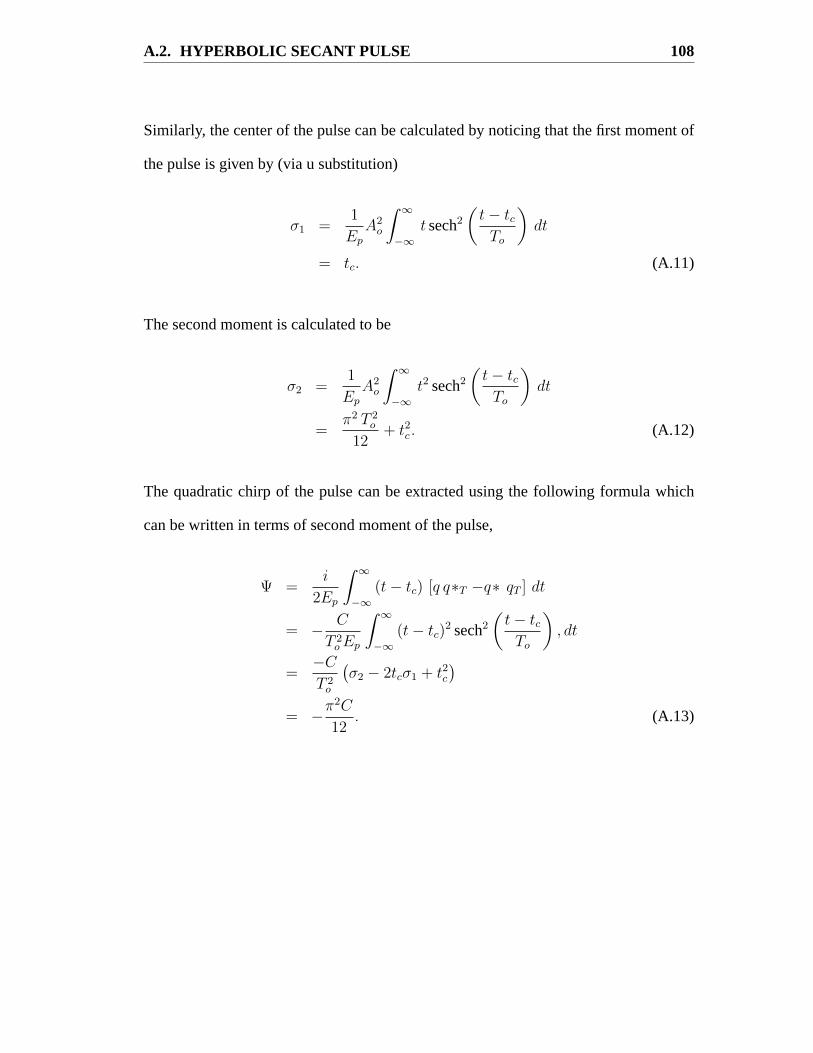
A.2. HYPERBOLIC SECANT PULSE 108
Similarly, the center of the pulse can be calculated by noticing that the first moment of
the pulse is given by (via u substitution)
σ1 =1
Ep
A2o
∫ ∞
−∞t sech2
(t− tcTo
)dt
= tc. (A.11)
The second moment is calculated to be
σ2 =1
Ep
A2o
∫ ∞
−∞t2 sech2
(t− tcTo
)dt
=π2 T 2
o
12+ t2c . (A.12)
The quadratic chirp of the pulse can be extracted using the following formula which
can be written in terms of second moment of the pulse,
Ψ =i
2Ep
∫ ∞
−∞(t− tc) [q q∗T −q∗ qT ] dt
= − C
T 2o Ep
∫ ∞
−∞(t− tc)
2 sech2(
t− tcTo
), dt
=−C
T 2o
(σ2 − 2tcσ1 + t2c
)= −π2C
12. (A.13)

109
Appendix B
Bit-Error Rate
In Chapter 5, we first introduced the parameter Q which approximates bit-error rate
(BER) to qualify system performance. We will now provide a more in depth derivation
of calculating BER [70].
BER is an excellent measurement of the system performance because it quantifies
the probability in which an error is made in the decision system. The error is often
due to the presence of various noises in the system. As a result, BER typically has a
strong dependence on the signal to noise ratio (SNR) of the signal received. A BER of
10−9 corresponds to 1 error per109 bits. Error-free transmission is often referred to as
having BER less than10−9, although modern systems often require BER to be less than
10−12. In a binary coding system, BER is merely the sum of probabilites of identifying
1 bit as 0 bit and vice versa. Mathematically, it is expressed as
BER = p(1) P (0/1) + p(0) P (1/0), (B.1)
wherep(1) andp(0) is the probability of receiving 1 and 0 bits respectively. P(0/1) is
the conditional probability of assigning a 0 bit to the signal when in actuality a 1 bit is

110
received and P(1/0) is the conditional probability of assigning a 0 bit to the signal when
in actuality a 1 bit is received.
In calculating the BER, two assumptions are made. First, it is safe to assume that in
any given pattern, the probability of receiving 1 and 0s is about the same. As such, we
can equatep(0) = p(1) = 0.5. The second assumption involves the probability density
function of the random process of received signals. For most systems not dominated
by inter-symbol interference (ISI), we can assume the random process to be Gaussian
with different average and variance for the 1 and 0 bits, i.e.,
p(m) =1
σm
√2π
exp
[−(I − Im)2
2σ2m
](B.2)
with Im and σm corresponding to the average current and variance for 1 or 0 bits,
depending onm = 0 or 1. Now we can evaluate the two conditional probabilities in
Eq. (B.1) as
P (0/1) =1
σ1
√2π
∫ ID
−∞exp
[−(I − I1)
2
2σ21
]dI (B.3)
P (1/0) =1
σ0
√2π
∫ ∞
ID
exp
[−(I − I0)
2
2σ20
]dI, (B.4)
whereID is the threshold setting between deciding whether a received signal is 1 or 0
bit. The above integral is in the form of the complementary error function defined by
erfc =2√π
∫ ∞
x
exp(−y2) dy. (B.5)

111
Evaluating Eqs. (B.3)–(B.4) using Eq. (B.5) simplify Eq. (B.1) into
BER =1
4
[erfc
(I1 − ID
σ1
√2
)+ erfc
(ID − I0
σ0
√2)
)]. (B.6)
It suffices to say that all system designers wish to minimize BER. Optimizing BER
with respect to the only free variable left,ID, yielded the following expression (creating
our new parameter, Q)
I1 − ID
σ1
=ID − I0
σ0
≡ Q. (B.7)
Under this condition, it is straight forward to write the decision threshold as
ID =σ0I1 + σ1I0
σ0 + σ1
, (B.8)
and Q as
Q =I1 − I0
σ1 + σ0
. (B.9)
This reduces the equation for BER as follows,
BER =1
2erfc
(Q√2
)≈ exp(−Q2/2)
Q√
2π, (B.10)
where the approximated is reasonably accurate forQ > 3.