Design of experiments for constitutive model selection ...

Modelling Simul. Mater. Sci. Eng.7 (1999) 253–273. Printed in the UK PII: S0965-0393(99)01663-0

Design of experiments for constitutive model selection:application to polycrystal elastoviscoplasticity

M F Horstemeyer†, D L McDowell‡ and R D McGinty‡† Center for Materials and Engineering Sciences, Sandia National Laboratories, Livermore,CA 94551-0969, USA‡ The George Woodruff School of Mechanical Engineering, Georgia Institute of Technology,Atlanta, GA 30332-0405, USA

Received 2 November 1998, accepted for publication 4 February 1999

Abstract. To bridge length scales in plastic flow of polycrystalline fcc metals, the salient featuresof 3D polycrystalline elastoviscoplasticity at the crystal level (mesoscale) were studied to determinethe relative influences on macroscale behaviour. This 3D study builds upon the 2D planar double-slip analysis performed by Horstemeyer and McDowell in which the relative influence of theconstitutive-law features on macroscale properties in polycrystal plasticity were quantified foroxygen-free, high-conductivity copper. The mesoscale constitutive-law features considered includesingle-crystal elastic properties, slip-system-level hardening law, latent hardening, slip-system-level kinematic hardening, and intergranular constraint relation. Volume-averaged macroscaleresponses included the effective flow stress, plastic spin, elastic moduli, hardening behaviour, andaxial extension (for the free-end torsion case). Each response was evaluated at 10% and 50%effective strain levels under rectilinear shear straining. In the existing literature, only one typeof behaviour (e.g. texture or stress–strain response) is typically considered when assessing thesevarious elements of the constitutive framework. In this paper, we develop a more comprehensiveunderstanding of the relative importance of constitutive-law features as deformation proceeds. Thisstudy suggests that the design of experiments methodology is a valuable tool to assist in selectingrelevant features for polycrystalline simulations and for development of macroscale unified-creep-plasticity models. In general, the results indicated that the intergranular constraint and kinematichardening were more influential overall than the type of constitutive model used, whether isotropicor anisotropic elasticity was used, and whether or not latent hardening was used. Finally, 3D resultswere similar to the previous 2D planar double-slip study of Horstemeyer and McDowell, except thatlatent hardening had a stronger influence on the 3D macroscale responses than the 2D macroscaleresponses.

1. Introduction

Continuum-slip polycrystal plasticity models have become quite popular in recent years asa tool to study deformation and texture behaviour of metals during processing (cf. Dawson(1987), Kalidindiet al (1992)) and shear localization (cf. Peirceet al (1982), Rashidet al(1992)). The basic elements of the theory consist of (i) slip-system hardening laws to reflectintragranular work hardening, including self- and latent-hardening components (Kocks 1976,1987) and (ii) intergranular constraint laws to govern interactions among grains. The theory isacknowledged for providing somewhat realistic prediction/correlation of texture developmentand stress–strain behaviour at large strains.

Different authors have developed or recommended various forms of the basic elementsof polycrystal plasticity theory that address specific applications, strain levels of interest and

0965-0393/99/020253+21$19.50 © 1999 IOP Publishing Ltd 253

254 M F Horstemeyer et al

so forth. To date, however, there has been no systematic application of objective principles todiscern the relative influence of various elements of the 3D theory on the collective macroscaleresponses. Hence, studies on different strain regimes and deformation paths have led todisparate conclusions regarding the relative importance and viability of specific forms ofhardening laws, constraint relations, and other elements of constitutive laws. In this paper,we present a ‘design of experiments’ (DOE) methodology to quantify the relative influenceof different theory elements on prediction of macroscale behaviour at various strain levels forrectilinear shearing. This methodology is intended primarily to give guidance as to whichattributes should receive critical attention and which are relatively insignificant in a givenapplication. Polycrystal elastoviscoplasticity is a good example of a highly nonlinear, coupledset of constitutive laws at the scale of individual grains which produces collective descriptionof behaviour over many grains that is not easily traced to assumptions at the primal scale.

The DOE approach was used to quantify relative differences between effects of variousmesoscale features on the macroscale volume-averaged (mean) polycrystalline responses.Such a method does not evaluate the accuracy of any given model, just the relative influence ofthe various nonlinear model features. The DOE approach was applied to a 2D planar double-slipelastoviscoplastic formulation (Horstemeyer and McDowell 1997) but has not been used for 3Dcrystal plasticity. Numerical results were correlated with the experimental torsional effectivestress-strain curves for oxygen-free, high-conductivity copper (OFHC Cu). Mesoscale modelfeatures (parameters in the DOE) considered included the single-crystal elastic properties,slip-system-level hardening law, latent hardening law, slip-system-level kinematic hardening,and the intergranular constraint relation. The volume-averaged macroscale responses includedthe effective flow stress, texture, plastic spin, elastic moduli, hardening behaviour, and axialstress (for the fixed-end torsion case). Each response was evaluated at 10% and 50% effectivestrain.

The DOE is a statistical analysis that employs orthogonality principles to evaluate therelative influence of mesoscale model features on the macroscale responses. This sensitivitystudy is the first of its type known to the authors applied to the various elements of 3Dpolycrystalline plasticity theory. Essentially, the DOE approach offers the capability to assessthe sensitivity of the macroscale model predications to various independent features of themesoscale constitutive relations. This methodology is not limited to polycrystalline metals,although that is the context of this article. After presenting the methodology, we consider theinfluence of various parameters:

(a) whether the single crystal elastic properties are isotropic or anisotropic;(b) the type of intergranular constraint employed: Taylor (1938) or finite-element method(c) effects of latent hardening versus Taylor hardening;(d) the form of hardening model used: Armstrong and Frederick (1966) or Rashid and Nemat

Nasser (1990);(e) whether or not slip-system kinematic hardening is used (Horstemeyer and McDowell

1997).

The responses given by the macroscale volume-averaged quantities (effective flow stress,work-hardening rate, plastic spin, elastic moduli, and axial extension) are then discussed.Finally, some comparisons with the planar double-slip study are discussed.

2. Statistical design of experiments technique

The earliest works that relate statistical procedures to physical experiments were due to SirRonald Fisher (1935a, b). As a result of his work, statisticians used several analysis of variance

DOE for model selection 255

techniques to interpret physical experimental data (Boxet al1978). DOE is one such technique.Taguchi (1974, 1986, 1987) popularized the DOE method for use in the quality-engineeringarea. Nelder and Lee (1991) discussed the use of linear statistical models for DOE analysis.Nair and Shoemaker (1990) reviewed various applications of the DOE. Nair (1992) led apanel discussion covering the mathematical and practical applications of DOE methods. Inthe present DOE study, the ‘experiments’ are not physical but numerical in nature.

An investigator can select a number of levels for each variable or parameter and then runexperiments to evaluate the parametric effect in an efficient manner. Hence, any number oflevels or parameters can be placed in an orthogonal array so as to efficiently determine theparametric effects. Orthogonality refers to statistically independent or balanced parameters thatmake up the columns of the array. Once the number of levels and parameters are determined,an orthogonal array is set up to determine the number of experiments needed (Taguchi 1986,1987). The terminology of orthogonal arraysLx(yz) is as follows. ‘x’ denotes the number ofcalculations in the experiment, ‘y’ denotes the number of levels, and ‘z’ denotes the numberof parameters. For example, to examine eight parameters at three levels, one would have anorthogonal array represented byL18(38) (cf. Taguchi (1986)) which would reduce the numberof calculations if performed linearly in series from 6561 to 18.

For the purposes of understanding the relative influence of the various polycrystallinemesoscale model features on macroscale responses, only two levels were chosen with fiveindependent variables. As such, the appropriate orthogonal array is theL8 array. TheL8

represents an orthogonal array of equations represented by eight ‘experiments’. TheL8 arrayallows up to seven independentparameterswith two levels for each parameter. Eachlevelcan be characterized by an appropriate attribute. For example, theparametercould be theintergranular constraint, and the twolevelsmight be defined by either the Taylor constraint(Taylor 1938) or use of the finite-element method. Although a full factorial set of calculationscould be performed to vary each parameter in a linear fashion, a DOE reduces the set ofcalculations in a repeatable, cost-effective manner such that data can be easily translated intomeaningful and verifiable conclusions. With this technique, relevant data can be extracted froma relatively small number of experiments (or numerical calculations). Clearly, the advantagesof DOE as a screening process for parameter influence grow exponentially as the number ofparameter variations increases. Table 1 shows theL8 array of calculations performed in thepresent example.

Table 1. L8 orthogonal array showing the parameters.

Kinematic Latent Hardening Intergranular ElasticCalculation hardening hardening model constraint properties

1 Yes 1.0 AF FEM Anisotropic2 Yes 1.0 AF Taylor Isotropic3 Yes 1.4 RNN FEM Anisotropic4 Yes 1.4 RNN Taylor Isotropic5 No 1.0 RNN FEM Isotropic6 No 1.0 RNN Taylor Anisotropic7 No 1.4 AF FEM Isotropic8 No 1.4 AF Taylor Anisotropic


3. Mesoscale influence parameters

In this section, we describe each parameter with its corresponding two levels. The term ‘modelfeature’ is used interchangeably with ‘parameter’ in this context since we have focussedon constitutive models. Before the model features are discussed, some explanation for thecrystalline kinematics is in order to show that all the model features are interdependent.For example in a current configuration formulation, three main coupled ordinary differentialequations need to be simultaneously solved, i.e.

σ = W eσ − σW e +C∗ :(D − Dp

)+C∗ :

[W

p(B∗ : σ

)−(B∗ : σ

)W

p]

(1)

D = De + Dp

+(B∗ : σ

)W

p− W p(B∗ : σ

)(2)

W = W e + Wp

+(B∗ : σ

)D

p− Dp(B∗ : σ

)(3)

whereσ is the Cauchy stress,D is the rate of deformation,W is the continuum spin,De isthe elastic rate of deformation,W e is the elastic spin,D

pis the plastic rate of deformation,

Wp

is the plastic spin,C∗ is the elastic moduli rotated to the current configuration, andB∗

is the elastic compliance rotated to the current configuration. The different terms arise whenthe multiplicative decomposition of the deformation gradient is divided into elastic (includingrigid lattice rotation) and plastic parts, i.e.F = F eF p.

F p is computed at the end of the time step by applying the Cayley–Hamilton theorem,

Fpt+1t = exp

(Lp1t

)F

pt (4)

whereF pt andF p

t+1t are the plastic deformation gradients at the beginning and end of the timestep, respectively.Lp is the plastic velocity gradient in the intermediate configuration thatoccurs during the time step, which is determined by (Asaro 1983)

Lp =N∑i=1

γi(si ⊗mi

)(5)

whereN is the number of slip systems, ˙γi is the continuum slip or shear rate on theith slipsystem,si is the slip direction vector, andmi is the slip-plane normal vector.

The focus of this paper is not to identify the absolute accuracy of specific models ofmicrostructural phenomena; many representations exist to model hardening, for example, thatmay be more accurate than either the Rashid–Nemat Nasser hardening rule or the Armstrong–Frederick (Armstrong and Frederick 1966) form used in this work. We focus instead on anobjective methodology by which we can assess the relative influence of various elements ormodel features within a complex, highly nonlinear and coupled constitutive framework suchas polycrystal plasticity. This is relevant to sorting out key mesostructure, macro-propertyrelationships that should receive particular attention in building up robust, physically basedmodels. Although humans (particularly experts!) can assimilate such relative comparisonsin manual fashion to a reasonable degree, such assessments are often biassed towards pre-conceived notions of proper model components or assemblages thereof. Specifically, inthe context of the hierarchical modelling ideas discussed by Olson (1997), we contendthat the DOE methodology may provide quantitative indication of cause-and-effect betweenmicro/mesostructure and performance at the macroscopic level, thereby focussing attention onthe most salient elements of evolving microstructure. As Olson puts it,

. . . much of materials science is the art of discriminating the essential from thenonessential. . . as weunravel the complex products of empirical development tocontrol desired properties. It is reciprocity that gives us the tools for materials design.


Olson mentions the reciprocity principle first elaborated by Cohen (1976), which statesthat although we typically regard properties as controlled by structure, we may also regardstructure as controlled by properties in terms of our conception or idealization of that structure.This permits us to distil simplicity from complexity by focussing on specific propertiesor performance attributes. In this case, we are interested in discerning the appropriatetools for modelling structure–property relations, assuming that mesoscale structure evolutionis represented in the phenomenological sets of grain-level constitutive laws. Orthogonalstatistical DOE methods are rather well suited for this algorithm. To proceed, it is necessary toidentify those macroscopic performance goals/parameters of most interest. Then, the relativeimportance of the microstructural model features changes as a function of the selected set ofmaterial performance indices.

We next consider examples of different mesoscale representations/models which will beused to examine relative effects on the macroscale response function of the polycrystallineaggregate. Those selected here for illustration are of a very well established, simple characterand are chosen to provide a wide range of description at the mesoscale (i.e. single grain orsmall sets of grains).

3.1. Isotropic versus anisotropic elasticity

Elastic properties arise from the binding forces of atoms as affected by the distance betweenthem. The elastic properties of single crystals can be highly anisotropic and can vary with theorientation of the crystal lattice.

The hyperelastic relation is specified in the intermediate, or stress-free, configuration as

σ(E)= C : E (6)

where the elastic stiffness tensor,C, is invariant for a given crystal in the intermediateconfiguration (cf. Asaro (1983)). The intermediate configuration is aligned with the crystallineaxes. σ is the second Piola–Kirchhoff stress in the intermediate configuration, andE is theconjugate Green elastic strain. For cubic orthotropy, the single-crystal elastic moduli areformed on axes of cubic symmetry (〈100〉, 〈010〉, and〈001〉 axes). By defining

C1 = C1111= C2222= C3333

C2 = C1122= C2233= C1133

C3 = C1212= C1313= C2323

(7)

the components are formed on the cartesian axes coincident with (〈100〉, 〈010〉, and〈001〉axes) with all otherCijkl equal to zero. The stress in the current configuration is related to thesecond Piola–Kirchhoff stress by

σ = 1

JF eσ F eT

. (8)

Now the Zener anisotropy factor as related to the crystal axis (not the specimen axis) isgiven by

Z = 2C3

C1− C2. (9)

WhenZ = 1, the elastic properties are isotropic; however,Z > 3 for Cu single crystals.In finite inelastic deformation, grains rotate and tend to align themselves statistically towarda pole. As each grain rotates, elasticity is considered to influence macroscale mechanicalbehaviour (Franceet al1967). Lowe and Lipkin (1990) showed that anisotropic single-crystalelastic properties are necessary for determining macroscale responses under non-monotonic


loading conditions at finite strain. Cuitino and Ortiz (1992) used anisotropic single-crystalelastic properties for a strain-localization problem. Alternatively, Rashidet al (1992), inthe spirit of Lin (1957), used isotropic single-crystal properties and showed that localization(and strain softening) does not depend on elastic anisotropy. None of these works comparedisotropic and anisotropic elasticity directly.

The elastic properties in this study are used to compare the influence of single-crystalisotropic versus anisotropic elasticity. The single-crystal elastic constants used are given intable A1 in the appendix.

3.2. Intergranular constraint relation

The intergranular constraint plays a crucial role in determining accurate macroscale responses(Honneff and Mecking 1978), since each grain is assumed to possess a distinct crystallographicorientation. Hence, the intergranular constraint controls the effects of crystallographicmisorientations among grains. In the DOE study we use a Taylor-type (Taylor 1938) constraintand the finite-element method as two different models. For each analysis, 198 randomlyoriented grains were used. The same deformation was applied to all the grains in the Tayloranalysis. For the finite-element analysis, a 2D plane strain finite-element mesh was used thatallowed 3D rotations for the crystals.

We used the finite-element code ABAQUS for our analyses, in which single-crystalorientations were used in different elements of the mesh (cf. Kalidindi and Anand (1991),Kalidindi et al (1992), Dawsonet al (1994)). By using finite elements, the constraintsamong grains will relax as deformation proceeds along the lines of a self-consistent modellingintroduced earlier by Hutchinson (1970). The mesh comprised 15 rows by 30 columns ofelements. Uniform uniaxial displacements were applied to the mesh. Only the responses ofthe central 198 elements/grains (9 rows by 22 columns) were included in the DOE study inorder to minimize the influences of the boundary conditions.

To solve the polycrystalline boundary-value problem using a single-crystal analysiswithout finite elements, an averaging procedure is needed which employs some assumption forthe intergranular constraint. A crystal-to-aggregate averaging theorem (Bishop and Hill 1951,Hill 1965, Hill and Rice 1972) was developed based on an assumption by Taylor (1938) that thedeformation gradient in each grain is the same. Other types of intergranular constraints havealso been assumed (cf. Eshelby (1957), Kroner (1961), Budiansky and Wu (1962), Honneffand Mecking (1978), Berveiller and Zaoui (1979), etc). The Taylor constraint produces anupper bound estimate for flow stress since it ensures compatibility but not equilibrium.

3.3. Hardening models with and without latent hardening

The viscoplastic kinetic relation used in this study is a kinematic hardening generalization ofthe form employed by Hutchinson (1976), i.e.

γi = γosgn(τi − αi)∣∣∣∣τi − αigi

∣∣∣∣M (10)

where the plastic slip rate on theith slip system, ˙γi , is a function of a fixed reference strainrate, ˙γo, the reference shear strength,gi , the resolved shear stress on the slip system,τi , the ratesensitivity exponent for the material,M, and an internal state variable representing kinematichardening effects resulting from backstress at the slip-system level,αi .

Two forms of the hardening law were chosen for evaluation in the DOE, the Armstrong–Frederick (Armstrong and Frederick 1966) and Rashid–Nemat Nasser model (Rashid and


Nemat Nasser 1990). The Armstrong–Frederick form contains an isotropic hardeningevolution law for the internal hardening state variable,gi , on ith slip system given by

gi = A12∑j=1

qij∣∣γj ∣∣− Bgi 12∑

j=1

∣∣γj ∣∣ (11)

whereA andB are the hardening and recovery moduli used to fit the experimental data, andqijis the latent hardening ratio that was set to 1.0 for Taylor hardening and 1.4 for stronger latenthardening in the DOE study. The self-hardening components arise wheni = j and the latenthardening components arise wheni 6= j . Note that for OFHC Cu the number of potential slipsystems is 12.

The increase or decrease in flow stress on a secondary slip system due to crystallographicslip on an active slip system is referred to as latent hardening. Taylor and Elam (1923),based on experimental evidence on aluminum crystals, observed that when latent hardeningequals self-hardening, an isotropic response exists. Kocks (1970) reviewed the behaviourof several materials under different loading conditions and surmised that an intersecting slipsystem induces higher stresses in the well-developed flow-stress regime. The latent hardeningratio, which is the ratio of hardening on the secondary system compared with the primarysystem, ranges from 1.0 to 1.4 for the form used by Hutchinson (1976) and Peirceet al (1982),sometimes called the PAN rule, where 1.0 corresponds to Taylor hardening.

Hansen and Jensen (1991) showed for tensile tests that texture and conventional latenthardening effects cannot account for all sources of anisotropy, in general. In essence, latenthardening models have focussed on dislocation–dislocation interactions, but in reality latenthardening arises from dislocation–substructure interactions as well. In the latter case, anevolving latent hardening ratio would be necessary. Although potentially important, anevolving latent hardening ratio is beyond the scope of this study. We employ the simplifiedPAN rule for latent hardening as

qij =[δij + lhr

(1− δij

)](12)

wherelhr is the latent hardening ratio, andδij is the Kronecker delta.Other latent hardening forms have been proposed and might be fruitful to consider in

such parameter studies; for example, Weng (1987) claimed that equation (12) is suitable formonotonic loadings but does not appropriately represent the forward and reverse interactions ofcrystallographic slip. Furthermore, it cannot distinguish between acute and obtuse cross slipsin reversed quasi-static loading conditions. Weng (1987) proposed a rate-independent, three-parameter model for latent hardening representing forest dislocation features that correlatedwith Phillips’ (Phillips and Gray 1961, Phillips and Kasper 1973, Phillips and Das 1985)measured initial and subsequent yield surfaces under combined stress fields. Havner (1982)employed a two-parameter rule of Nakada and Keh (1966) to examine latent hardening effects,showing that the contribution of incremental slip from self-hardening equals that of the latentsystem. Bassani and Wu (1991) have introduced a self-hardening formulation that has capturedsome of the apparent latent hardening effects.

Other issues regarding latent hardening that are not included in this work includedifferences that have been observed from one latent system to the next. Franciosiet al (1980)determined in Cu and Al single crystals that slip systems in which dislocations can form sessilejunctions appear to exhibit primary latent hardening. Secondary latent hardening is associatedwith systems for which dislocations form glissile junctions or Hirth locks with those of theactive slip systems. Also not considered is the influence of the stacking-fault energy; the lowerthe stacking-fault energy, the higher the latent hardening. Models to date only empirically fitconstants to the latent hardening equation and physical motivation is often lacking. Finally,


although the latent hardening ratio seems to be independent of temperature, alloy type, andstrain rate (Kocks 1970), it does change during deformation, saturating at a strain of the orderof unity. In this study,lhr = 1.0 andlhr = 1.4 as shown in table 1.

Like the Armstrong–Frederick form, the Rashid and Nemat Nasser (1990) isotropichardening rule is given with the latent hardening ratio as

gi =

h0 06 γ 6 γ012∑j=1

h0qij∣∣γj ∣∣

1 +8(∣∣γj ∣∣− γ0

) γ0 6 γ(13)

whereh0,8, andγ0 are material constants.

3.4. Slip-system-level isotropic–kinematic hardening or isotropic hardening

The role of grain-level kinematic hardening was examined in this DOE study to assess itscomparative influence on the macroscale responses. Kinematic hardening at the grain level isused to model dislocation substructure contribution to the directional dislocation resistance.Kinematic hardening at the level of the slip system has been rather widely employed to describestrengthening due to heterogeneous dislocation substructure and attendant Bauschinger effects(cf. Jordan and Walker (1992)). We employ a substructural internal variable evolution equation(Horstemeyer and McDowell 1998). From the work of Horstemeyer and McDowell (1998),calculations were performed that illustrated the effects of the single-crystal kinematic hardeningon texture evolution and stress–strain behaviour. For the Armstrong–Frederick and Rashid–Nemat Nasser forms, we employ the following equation for each crystal

αi = Crate

(Csatγ

i− αi ‖γi‖

)(14)

whereCrate controls the rate of evolution, andCsat is the saturation level of the backstress,where these were chosen to fit the experimental data. The substructural hardening internalstate variable reflects dislocation interactions within the grain (cf. Rice (1971)) and followsthe postulate of Coleman and Gurtin (1967) that the rate must be governed by a differentialequation in which the plastic rate of deformation appears.

We note that a saturation value for the kinematic hardening was chosen to be about 20%of the effective flow stress at 30% strain. If the saturation value occurred at a lower strain levelor higher strain level, the conclusions of this DOE study might be different. However, thislevel of kinematic hardening is deemed physically consistent with substructure formation inpure metals and considerably less than that which might be produced in complex two-phasemicrostructures (cf. Kocks (1976, 1987)). For non-zeroα, the flow rule in equation (14) isused and in the DOE represents ‘yes’. When kinematic hardening is ‘no’ in table 1,α = 0.

It is well known that a certain degree of kinematic hardening (Bauschinger effect) isintroduced by virtue of the orientation dependence of grains and compatibility requirementsamong them in polycrystal plasticity theory. However, this is a highly transient effect thatoccurs over small cumulative plastic strain following a strain reversal. More persistentBauschinger effects arise from prescription of kinematic hardening at the scale of individualgrains (slip systems), affecting slip-system flow rules. Reversed-loading experiments on singlecrystals of both precipitate-strengthened (cf. Jordanet al1993) and pure metals (cf. Mughrabi1978) exhibit kinematic hardening due to heterogeneous inelastic flow. Precipitates offer aclear source of the behaviour in the former. Dislocation substructures induce these effects inthe latter. In the latter case, the backstress is induced by the collective effects of interactionswith dislocation structures at higher scales.


4. Macroscale responses

Certainmacroscaleresponses (attributes) were used to assess the relative importance of themesoscalemodel features. Essentially, these responses serve as performance indices or require-ments at the macroscale. One such macroscale response is the polycrystalline effective (vonMises) flow stress, which was correlated with the experimental data under free-end torsion con-ditions based only on the first-order response, i.e.σ eff = √3σ ave

12 . Each of the eight calculationswas correlated with the torsional data and remained at least within 6% of the stress level through-out the straining period. Table 2 summarizes the effective flow-stress levels at 10% and 50%strain for the eight calculations and the experimental data to illustrate the close approximations.

Table 2. Effective (von Mises) stress (MPa) from calculations and from experimental torsionaldata for OFHC Cu.

Calculation 10% eff. strain 50% eff. strain

1 130 2412 128 2413 132 2514 128 2405 123 2356 123 2367 121 2418 121 241Exp. result 123 240

Table A1 in the appendix summarizes the material constants that were used to determinethese stress–strain responses. We note that the material constants are not unique.

Another macroscale response is the plastic spin that is related to texture. We employaspects from the orientation distribution function (ODF), which depicts the evolution of textureas a function of effective strain. The ODF has two components: mean and spread, the meanbeing defined by the volume average over the polycrystalline distribution and the spread(assuming Gaussian distribution) being defined by the standard deviation of the polycrystallinedistribution. Horstemeyer and McDowell (1997) showed how this procedure was used torelate the pole and distribution of texture to the mean and spread of plastic spin and the work-hardening rate. Other macroscale responses of interest were the polycrystalline elastic moduliand development of polycrystalline axial extension in free-end shear which were determinedby the volume averages of the single-crystal quantities.

From theL8 array, we may write

[R] = [P ][A] (15)

where [R] is the response matrix, [A] is the output matrix and indicates the relative influenceof the crystal plasticity model feature, and [P ] is the parameter matrix. Each is denoted by

[R] =

R1

R2

R3

R4

R5

R6

R7

R8

[A] =

2A1

A2

A3

A4

A5

A6

A7

A8

[P ] =

+1 +1 −1 −1 −1 −1 +1 +1+1 +1 −1 −1 +1 +1 −1 −1+1 +1 +1 +1 −1 −1 −1 −1+1 +1 +1 +1 +1 +1 +1 +1+1 −1 −1 +1 −1 +1 −1 +1+1 −1 −1 +1 +1 −1 +1 −1+1 −1 +1 −1 −1 +1 +1 −1+1 −1 +1 −1 +1 −1 −1 +1

(16)


The parameter matrix [P ], shown in equation (16), has an equal number of occurrences ineach column. For each level within a column, each level within any other column will occuran equal number of times as well. This introduces the statistical independence or balance intothe orthogonal array. If the results, [R], associated with one level change to another level,then the parameter from one level to another has a strong impact on the macroscale responsebeing considered. Because different levels occur an equal number of times, an effect on themacroscale response by the other parameters is cancelled out. Hence, the−1’s and +1’s inmatrix [P ] are simply used to express the effect of the two different levels.

The values for theR-matrix, for example, for torsional effective stresses are given intable 2. The mean of the results from the DOE analysis is given byA1. A2 is the output fromthe eight calculations under the parameter related to the slip-system-level kinematic hardening.A3 reflects influence from latent hardening.A4 depends on the type of hardening model that wasused.A5 relates to the type of intergranular constraint used.A6 relates to the single-crystalelastic moduli that were used. DOE outputsA7–A8 are the outputs related to the second-order interaction of parameters. These second-order responses turned out to be negligible inthe analysis. Note thatA1–A8 do not have physical significance in an absolute sense, juststatistical significance in expressing the relative influence of associated model features on theresponse matrix,R. Furthermore, we note that we are assuming a statistical linear dependenceof terms so only two levels of each parameter were chosen. If more levels are desired, anotherorthogonal array would be necessary and a higher-order statistical assumption would have tobe made.

The matrix of outputs, [A], can be determined by inverting the parameter matrix, [P ].In the parameter matrix,−1 is placed where kinematic hardening is ‘no’ (recall table 1).The same is done when latent hardening is ‘1.0’, when the hardening model is AF, when theintergranular constraint is FEM, and when the elastic properties are anisotropic. In contrast,+1 is placed in the table when the kinematic hardening is ‘yes’, and so on. Since the response isdetermined from the finite-element calculations and is hence known, the DOE outputsA1–A8

can be determined from equation (16). These outputs are then used to quantify the parametriceffects of the model features.

4.1. Example: effective stress at 50% effective strain

For the sake of brevity, an example is presented of a macroscale response (effective flow stress)to illustrate the methodology, corresponding to 50% strain. The details of the determinationof the output values for the other macroscale responses will not be discussed later in thepaper, only the results. For the effective stress response at 50% strain, the kinematic outputlevelA2 = 20, the latent hardening output levelA3 = 20, the hardening model output levelA4 = 2, the intergranular constraint output levelA5 = 10, and the elastic properties outputlevelA6 = 12. Since these values arise relative to each other, the values were normalized tothe largest value among them in order to assess the relative level of influence of each parameter.Table 3 shows the values for the outputs when examining the effective stress level. ConstantA1 is the average and is not relevant to our parametric study so is not included in the discussion.

Hence, the most influential model features at 50% effective strain, when examining theeffective stress, were the kinematic hardening and latent hardening. The gradation that willbe used to describe the magnitude of influence is: (a) primary: 85–100%; (b) secondary:60–85%; (c) tertiary: 30–60%; (d) minor: 20–30%; (e) negligible: 0–20%.

Since the kinematic hardening and latent hardening have the highest statistical value, theyare the primary influence on the effective stress at 50% strain. The intergranular constraint andeffects of elasticity have a tertiary influence, and the effect of the hardening model is negligible.


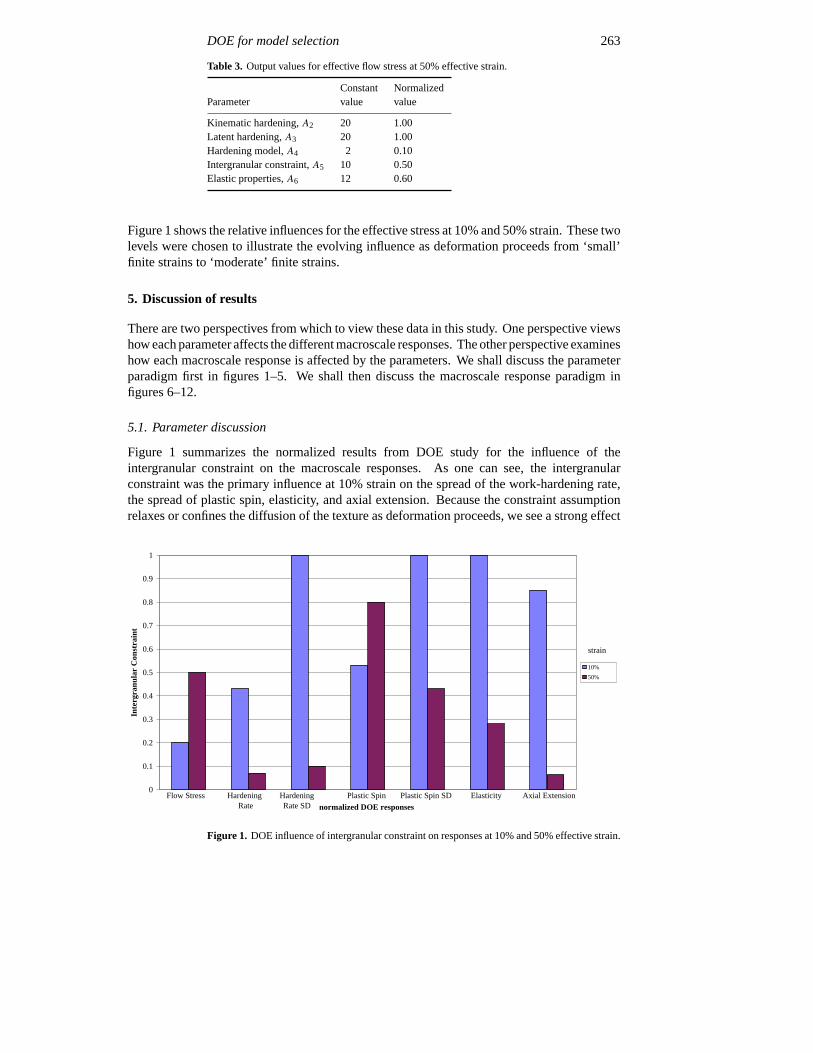
Table 3. Output values for effective flow stress at 50% effective strain.

Constant NormalizedParameter value value

Kinematic hardening,A2 20 1.00Latent hardening,A3 20 1.00Hardening model,A4 2 0.10Intergranular constraint,A5 10 0.50Elastic properties,A6 12 0.60

Figure 1 shows the relative influences for the effective stress at 10% and 50% strain. These twolevels were chosen to illustrate the evolving influence as deformation proceeds from ‘small’finite strains to ‘moderate’ finite strains.

5. Discussion of results

There are two perspectives from which to view these data in this study. One perspective viewshow each parameter affects the different macroscale responses. The other perspective examineshow each macroscale response is affected by the parameters. We shall discuss the parameterparadigm first in figures 1–5. We shall then discuss the macroscale response paradigm infigures 6–12.

5.1. Parameter discussion

Figure 1 summarizes the normalized results from DOE study for the influence of theintergranular constraint on the macroscale responses. As one can see, the intergranularconstraint was the primary influence at 10% strain on the spread of the work-hardening rate,the spread of plastic spin, elasticity, and axial extension. Because the constraint assumptionrelaxes or confines the diffusion of the texture as deformation proceeds, we see a strong effect

0

0.1

0.2

0.3

0.4

0.5

0.6

0.7

0.8

0.9

1

normalized DOE responses

Inte

rgra

nula

r C

onst

rain

t

10%

50%

Flow Stress Hardening Rate

Hardening Rate SD

Plastic Spin Plastic Spin SD Elasticity Axial Extension

strain

Figure 1. DOE influence of intergranular constraint on responses at 10% and 50% effective strain.


0

0.1

0.2

0.3

0.4

0.5

0.6

0.7

0.8

0.9

1


Kin

emat

ic H

arde

ning

10%

50%

Flow Stress HardeningRate

Hardening Rate SD

Plastic Spin Plastic Spin SD

Elasticity Axial Extension

strain

Figure 2. DOE influence of kinematic hardening on responses at 10% and 50% effective strain.

on the distribution spread of the plastic spin and work-hardening rate. These two macroscaleresponses are directly a function of the texture evolution. The influence of the intergranularconstraint is lessened as deformation proceeds.

The kinematic hardening had the most influence over the macroscale responses, more thanany other feature of the model at both levels of strain examined (10% and 50% ). Figure 2shows that primary influence over flow stress, axial extension, plastic spin, elasticity at a lowerstrain, and plastic spin spread at a higher strain. It had much less influence on the mean andspread of the work-hardening rate. This is interesting since the kinematic hardening saturated

0

0.1

0.2

0.3

0.4

0.5

0.6

0.7

0.8

0.9

1


Har

deni

ng R

ule

10%

50%


Hardening Rate SD


strain

Figure 3. DOE influence of hardening rule on responses at 10% and 50% effective strain.


0

0.1

0.2

0.3

0.4

0.5

0.6

0.7

0.8

0.9

1


late

nt h

arde

ning

10%

50%


Hardening Rate SD

Plastic Spin Plastic Spin SD

Elasticity Axial Extension

strain

Figure 4. DOE influence of latent hardening on responses at 10% and 50% effective strain.

at 30% strain indicating its continued influence on the memory of the material up to 50% strainand even being the primary influence at that point. This was also observed in the planar 2DDOE analysis of Horstemeyer and McDowell (1997).

The hardening rule had a primary influence on the work-hardening rate, mean plastic spin,and axial extension at 10% strain as shown in figure 3. The influence of the hardening rulechanged at 50% strain. It still had a primary influence on the work-hardening rate, but had anegligible influence on the mean plastic spin and axial extension. Otherwise at 50% strain, it

0

0.1

0.2

0.3

0.4

0.5

0.6

0.7

0.8

0.9

1


elas

tic

mod

uli

10%

50%


Hardening Rate SD


strain

Figure 5. DOE influence of elastic moduli on responses at 10% and 50% effective strain.


had a primary influence on the spread of plastic spin and work-hardening rate. This is interestingbecause it indicates that the hardening rule affects texture which in turn influences these twomacroscale quantities. The hardening rule had negligible effects on the polycrystalline elasticmoduli and surprisingly on the flow stress.

Figure 4 shows that the latent hardening parameter had a primary influence on the plasticspin throughout deformation. It had an increasing influence from negligible to primary onthe macroscale flow stress from 10% strain to 50% strain. By contrast, it had a decreasinginfluence from primary to negligible on the axial extension. On the hardening rate, elasticity,and spread of plastic spin the latent hardening influence was minimal to negligible.

The strongest influence on the polycrystalline elastic moduli was determined by whetherthe single-crystal elastic properties were anisotropic or isotropic, as shown in figure 5; this alsohad a primary influence on the plastic spin at 10% strain. It also had a secondary influenceon the axial extension at 10% strain but decreased at 50% strain. Otherwise, it had minor-to-negligible effects on the other macroscale responses.

5.2. Macroscale response discussion

The macroscale effective flow stress was determined by taking the volume average of the in-plane shear component and then applying the von Mises criterion, i.e.σ eff = √3σ ave

12 . Figure 6shows that at 10% and 50% effective strain, the kinematic hardening had the primary influence.At 10% strain, every other parameter had a negligible influence. At 50% strain, although thekinematic hardening had a primary influence on the flow stress, it saturated at 30% strain. Thisindicates a memory effect still influencing the material. At 50% strain, we also see that latenthardening had a primary influence whereas at 10% strain, it was negligible. Elasticity andintergranular constraint increased in influence to a tertiary level as the applied deformationincreased to 50% strain. The influence of the hardening rule was negligible.

0

0.1

0.2

0.3

0.4

0.5

0.6

0.7

0.8

0.9

1

parameters

norm

aliz

ed D

OE

flo

w s

tres

s re

spon

se

10%

50%

KinematicHardening

Latent Hardening

Hardening Rule IntergranularConstraint

Elasticity

strain

Figure 6. DOE polycrystalline flow stress results showing the relative influence of mesoscaleparameters at 10% and 50% effective strain.


0

0.1

0.2

0.3

0.4

0.5

0.6

0.7

0.8

0.9

1

parameters

norm

aliz

ed D

OE

wor

k ha

rden

ing

rate

res

pons

e

10%

50%

Kinematic Hardening

Latent Hardening

Hardening Rule Intergranular Constra

Elasticity

strain

Figure 7. DOE polycrystalline mean work-hardening rate results showing the relative influence ofmesoscale parameters at 10% and 50% effective strain.

Figures 7 and 8 show the responses of the mean and spread of the work-hardening rate as afunction of the parameters at 10% and 50% strain. The polycrystalline work-hardening rate isdefined by∂σ eff/∂εeff . The hardening rule was the dominant influence on the mean and spreadof the work-hardening rate. Interestingly, figures 7 and 8 show decreases in influence fromlatent hardening, intergranular constraint and elasticity from mainly a tertiary to a negligibleinfluence as the applied deformation proceeded from 10% to 50% strain. The kinematichardening had a negligible influence on the mean and spread of the work-hardening rate at

0

0.1

0.2

0.3

0.4

0.5

0.6

0.7

0.8

0.9

1

parameters

norm

aliz

ed D

OE

wor

k ha

rden

ing

rate

spr

ead

resp

onse

10%

50%

Kinematic Hardening

Latent Hardening

Hardening Rule Intergranular Constraint

Elasticity

strain

Figure 8. DOE polycrystalline spread of work-hardening rate results the relative influence ofmesoscale parameters at 10% and 50% effective strain.


0

0.1

0.2

0.3

0.4

0.5

0.6

0.7

0.8

0.9

1

parameters

norm

aliz

ed D

OE

pla

stic

spi

n re

spon

se

10%

50%bk

KinematicHardening

Latent Hardening


Elasticity

strain

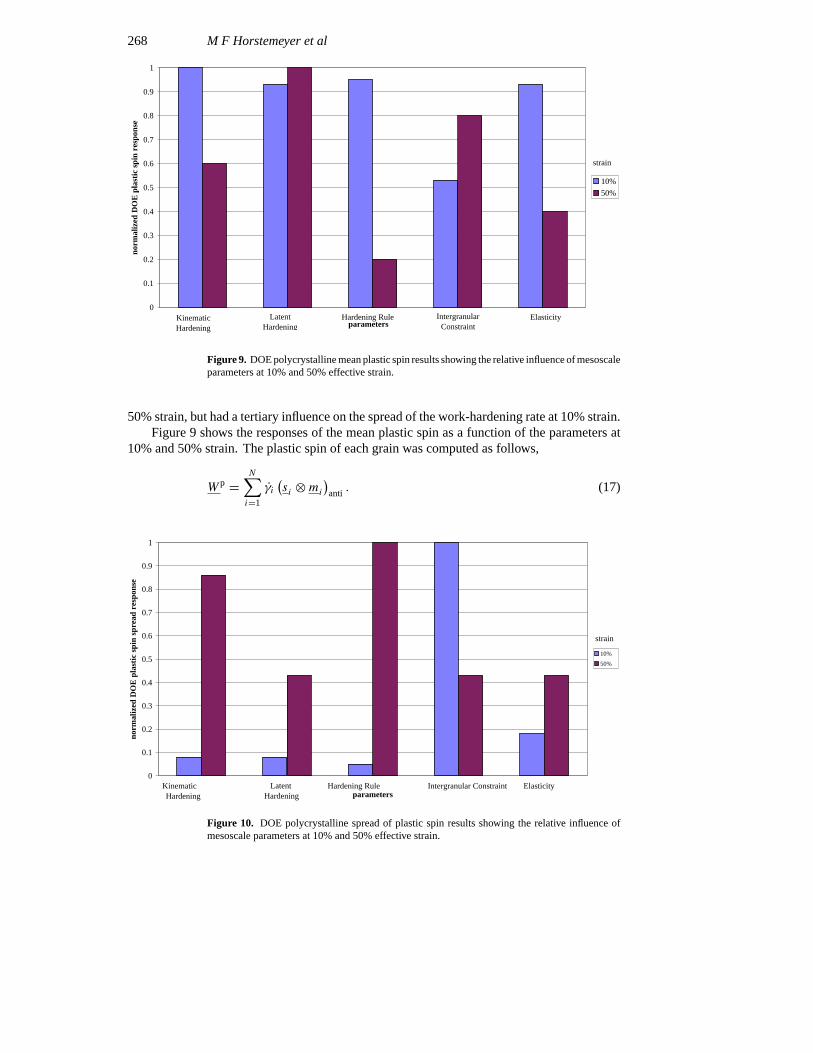
Figure 9. DOE polycrystalline mean plastic spin results showing the relative influence of mesoscaleparameters at 10% and 50% effective strain.

50% strain, but had a tertiary influence on the spread of the work-hardening rate at 10% strain.Figure 9 shows the responses of the mean plastic spin as a function of the parameters at

10% and 50% strain. The plastic spin of each grain was computed as follows,

W p =N∑i=1

γi(si ⊗mi

)anti . (17)

0

0.1

0.2

0.3

0.4

0.5

0.6

0.7

0.8

0.9

1

parameters

norm

aliz

ed D

OE

pla

stic

spi

n sp

read

res

pons

e

10%

50%

Kinematic Hardening

LatentHardening

Hardening Rule Intergranular Constraint Elasticity

strain

Figure 10. DOE polycrystalline spread of plastic spin results showing the relative influence ofmesoscale parameters at 10% and 50% effective strain.


0

0.1

0.2

0.3

0.4

0.5

0.6

0.7

0.8

0.9

1

parameters

norm

aliz

ed D

OE

ela

stic

ity

resp

onse

10%

50%

KinematicHardening

Latent Hardening


Elasticity

strain

Figure 11. DOE polycrystalline elastic shear moduli results showing the relative influence ofmesoscale parameters at 10% and 50% effective strain.

Since the macroscopic shear was imposed in the 1–2 direction, onlyWp12 has been reported.

The mean plastic spin is the numerical average of the individual grain values. Surprisingly,all the parameters had a relatively similar influence on the mean plastic spin as illustrated infigure 9. At 10% strain, the kinematic hardening, latent hardening, hardening rule, and elasticanisotropy all had a primary influence. The intergranular constraint had a tertiary influence at10% strain. This indicates a tight coupling of the equations in determining the plastic spin.At 50% strain, the intergranular constraint and latent hardening had primary influences, asthe influence of the kinematic hardening decreased to a secondary level. The influence of theelastic anisotropy decreased from a primary to a minor influence from 10% to 50% strain, andthe hardening rule decreased from a primary to negligible influence from 10% to 50% strain.

Figure 10 shows that the primary influence on the spread of the distribution of plastic spinat 10% strain was the intergranular constraint with all the other factors being negligible. At 50%strain, the kinematic hardening and hardening rule surprisingly had primary influences. Theintergranular constraint influence decreased to a tertiary level at 50% strain. Latent hardeningand elasticity had negligible influences on the spread of plastic spin at 10% strain but increasedto tertiary levels at 50% strain.

Figure 11 shows the responses of the polycrystalline elastic shear modulus as a functionof the parameters at 10% and 50% strain. The polycrystalline elastic moduli were determinedfrom the volume average over all the grains. As might be expected, the single crystal elasticmoduli had a strong influence on the polycrystalline elastic moduli throughout the deformation,but more so at 50% strain because of the deformation-induced anisotropy. At 10% effectivestrain, the intergranular constraint and kinematic hardening played a primary role but lostinfluence to only a minor role at 50% strain. The latent hardening and hardening rule hadnegligible effects on the polycrystalline elastic shear modulus.

Figure 12 shows the responses of the axial extension as a function of the parameters at10% and 50% strain. The polycrystalline axial extension developed during free-end shearingwas determined by the volume average of the single-crystal axial extension. Note that allthe parameters had a primary influence on the axial extension at 10% strain, but only the


0

0.2

0.4

0.6

0.8

1

1.2

parameters

norm

aliz

ed D

OE

axi

al e

xten

sion

res

pons

e

10%

50%

Kinematic Hardening Latent Hardening Hardening RuleH d i R l

Intergranular Constraint Elasticity

strain

Figure 12. DOE polycrystalline axial extension results showing the relative influence of mesoscaleparameters at 10% and 50% effective strain.

kinematic hardening retained a primary influence at 50% strain. At 50% strain the otherparameters decreased such that they had a negligible influence.

The results in Figure 12 are similar to those for the plastic spin. Axial extension forfree-end shear is a second-order effect and would be a result of the texture development likethe plastic spin. This result is critical when considering the modelling of secondary responses,such as axial extension in free-end shear or axial stresses in fixed-end shear, with macroscaleunified-creep-plasticity models. The axial stresses under fixed-end torsion and axial strainsunder free-end torsion have been attributed to texture effects (Harrenet al 1989).

5.3. Comparison of planar double-slip with three-dimensional results

Horstemeyer and McDowell (1997) performed a similar DOE analysis in a planar double-slipcontext, and it is instructive to compare those results with these 3D results. Both studiesshowed that the intergranular constraint and kinematic hardening had the most influence onthe macroscale parameters, but the 3D study showed a much stronger influence from latenthardening on the macroscale responses than the 2D study. This is somewhat surprisingconsidering the differences in the two formulations. First, there is the obvious differencethat the 2D double-slip formulation overconstrains the plasticity framework more than the 3Dframework. Another difference was that the boundary condition in the 2D study was fixed-endshear while in the 3D study it was free-end shear. A self-consistent method was also used inthe 2D study to relax the Taylor constraints but the finite-element method was used in the 3Dstudy. Finally, the form of one of the hardening rules changed from the Chang–Asaro (Changand Asaro 1981) hardening rule to the Armstrong–Frederick (Armstrong and Frederick 1966)hardening-recovery format. Even with these differences, the conclusions in the two studieswere very similar with qualitative differences, only occurring in relation to the influence oflatent hardening.


6. Summary

For a given materialandfor the given range of model features employed in this study, the DOEmethodology has quantified the relative influence of different selected elements of standardpolycrystal plasticity theory as a function of deformation level and path. Within this context,for the specific mesoscale constitutive relations selected for the study some key findings includethe following.

• The introduction of kinematic hardening at the scale of individual grains (slip system)demonstrated a strong influence on the polycrystal flow stress, mean and spread of plasticspin, polycrystalline elastic shear modulus, and axial extension. The kinematic hardeninghad minor-to-negligible influences on the mean and spread of the work-hardening rate.In spite of the fact that kinematic hardening was introduced as a short range transientthat saturated at 20% of the effective flow stress after 30% effective strain in monotonicdeformation, it still had influence up to 50% strain.• The intergranular constraint had a strong influence on the spread of the polycrystal work-

hardening rate and plastic spin. At 10% strain, the intergranular constraint had a primaryinfluence on the polycrystalline elastic moduli and on the axial extension.• The choice of latent hardening had a greater influence in the 3D study than in the previous

2D study of Horstemeyer and McDowell (1997). The latent hardening played a primaryrole in the polycrystalline flow stress, mean plastic spin, and axial extension. It had atertiary role in the mean and spread of the polycrystalline work-hardening rate and spreadof plastic spin.

The range of constitutive model elements was not exhaustive in this study. For example,the results were indifferent to latent hardening for values ofq = 1 or q = 1.4 for thePeirce–Asaro–Needleman formulation for both texture and stress–strain behaviour in shearand compression for OFHC Cu. Of course, the influence of this model in comparison with aradically different formulation of latent hardening (cf. Weng (1987)) might prove to be quitesignificant. Furthermore, a material such as aluminum, which has a lower hardening rate thancopper and is more elastically isotropic, may generate different results.

In this study, only shear loading paths were considered. For reversed yielding or changesof the deformation path even more demanding, discriminatory requirements are placed on theelements of the constitutive models. The DOE methodology could be used for this type ofloading path as well as a straightforward extension.

We emphasize that this DOE methodology provides the relative influence or the sensitivityof an aggregate performance index or response function to a range of mesoscale models forevolving structure and its effects. As such, the methodology may be useful as part of an overallstrategy for optimization of constitutive laws that covers not only parameter estimation, but alsothe objective selection of the forms of the various elements such as hardening and constraintlaws. Polycrystal plasticity is a good example of a nonlinear constitutive law with multiplesources and scales of nonlinearity. Generally, models that attempt to bridge vastly differentlength scales exhibit the same kind of amenability to the DOE approach. The results arealso useful in guiding the disposition of effort to improve certain elements in order to achieveenhanced description. For example, if the precise form of the slip-system hardening rule doesnot significantly influence the macroscale average response function, then there is little impetusto refine it further, unless the form (e.g. dependent variables) is radically different. This sortof information is of an entirely different character to that offered by parameter optimizationschemes, where the objective is to find a set of parameters that minimizes some error normover the space of desired performance objectives for aspecificconstitutive model structure.


Acknowledgments

The work by M F Horstemeyer was performed under the U.S. Department of Energy contractnumber DE-AC04-94AL85000. D L McDowell and R McGinty are grateful for the support ofthe U.S. Army Research Office (Dr K Iyer, Program Manager) in conducting this and relatedresearch.

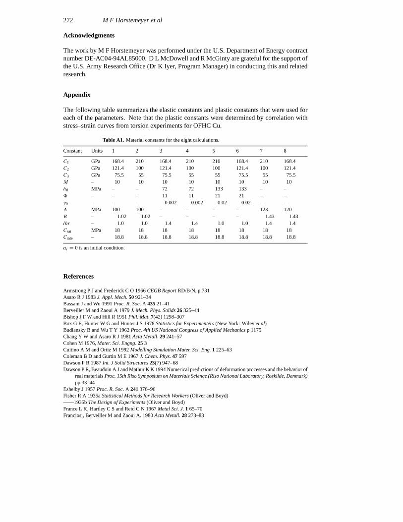
Appendix

The following table summarizes the elastic constants and plastic constants that were used foreach of the parameters. Note that the plastic constants were determined by correlation withstress–strain curves from torsion experiments for OFHC Cu.

Table A1. Material constants for the eight calculations.

Constant Units 1 2 3 4 5 6 7 8

C1 GPa 168.4 210 168.4 210 210 168.4 210 168.4C2 GPa 121.4 100 121.4 100 100 121.4 100 121.4C3 GPa 75.5 55 75.5 55 55 75.5 55 75.5M – 10 10 10 10 10 10 10 10h0 MPa – – 72 72 133 133 – –8 – – – 11 11 21 21 – –γ0 – – – 0.002 0.002 0.02 0.02 – –A MPa 100 100 – – – – 123 120B – 1.02 1.02 – – – – 1.43 1.43lhr – 1.0 1.0 1.4 1.4 1.0 1.0 1.4 1.4Csat MPa 18 18 18 18 18 18 18 18Crate – 18.8 18.8 18.8 18.8 18.8 18.8 18.8 18.8

αi = 0 is an initial condition.

References

Armstrong P J and Frederick C O 1966CEGB ReportRD/B/N, p 731Asaro R J 1983J. Appl. Mech. 50921–34Bassani J and Wu 1991Proc. R. Soc. A 43521–41Berveiller M and Zaoui A 1979J. Mech. Phys. Solids26325–44Bishop J F W andHill R 1951Phil. Mat. 7(42) 1298–307Box G E, Hunter W G and Hunter J S 1978Statistics for Experimenters(New York: Wileyet al)Budiansky B and Wu T Y 1962Proc. 4th US National Congress of Applied Mechanicsp 1175Chang Y W and Asaro R J 1981Acta Metall. 29241–57Cohen M 1976,Mater. Sci. Engng. 253Cuitino A M and Ortiz M 1992Modelling Simulation Mater. Sci. Eng.1 225–63Coleman B D and Gurtin M E 1967J. Chem. Phys.47597Dawson P R 1987Int. J Solid Structures23(7) 947–68Dawson P R, Beaudoin A J and Mathur K K 1994 Numerical predictions of deformation processes and the behavior of

real materialsProc. 15th Riso Symposium on Materials Science (Riso National Laboratory, Roskilde, Denmark)pp 33–44

Eshelby J 1957Proc. R. Soc. A 241376–96Fisher R A 1935aStatistical Methods for Research Workers(Oliver and Boyd)——1935bThe Design of Experiments(Oliver and Boyd)France L K, Hartley C S and Reid C N 1967Metal Sci. J. 1 65–70Franciosi, Berveiller M and Zaoui A. 1980Acta Metall. 28273–83


Hansen N and Jensen J D 1991 Anisotropy and localization of plastic deformationProc. 3rd Symposium on Plasticityand Its Current Applicationsed J P Boehler and A S Khan, pp 131–4

Harren S, Lowe T C, Asaro R J and Needleman A 1989Phil. Trans. R. Soc. A 238443–500Havner K S 1982Mech. Mater. 1 97–111Hill R 1965J. Mech. Phys. Solids1389–101Hill R and Rice J R 1972J. Mech. Phys. Solids20401–13Honneff W G and Mecking H 1978Texture of Materialsed G Gottstein and K Lucke (Berlin: Springer) pp 265–75Horstemeyer M F and McDowell D L 1997 Using statistical design of experiments for parameter study of crystal

plasticity modeling features under different strain pathsSandia National Laboratories ReportSAND96-8683——1998Mechanics of Materialsat pressHughes D A 1995Proc. 16th Riso International Symposium (Roskilde, Denmark)ed N.Hansenet alHutchinson J W 1970Proc. R. Soc. A 319247–72——1976Proc. R. Soc. A 348101–27Jordan E H and Walker K P 1992J. Engng Mater. Tech. 11419–26Jordan E H, Shi S and Walker K P 1993Int. J. Plasticity9 119–39Kalidindi S R and Anand, L. 1991Advances in Finite Deformation Problems in Materials. Processing and Structures

1253–14Kalidindi S R, Bronkhurst C A and Anand L 1992J. Mech. Phys. Solids40(3) 537–69Kocks U F 1970Metall. Trans. 1 1121——1976J. Engng Mater. Tech. 9876–85——1987Unified Constitutive Equations for Creep and Plasticityed A K Miller (New York: Elsevier) ch 1, pp 1–88Kroner E 1961Acta Metall. 9 155Lin T H 1957J. Mech. Phys. Solids5 143Lowe T C and Lipkin J 1990 Analysis of axial deformation response during reverse shearSandia National Laboratories

ReportSAND90-8417McDowell D L, Miller M P and Bammann D F 1991 Some additional considerations for coupling of material and

geometric nonlinearities for polycrystalline metalsProc. MECAMAT ’91 (Fontainebleau, France)Miller M P 1993PhD ThesisGeorgia Institute of TechnologyMughrabi H 1978Mater. Sci. Engng33207–23Nakada Y and Keh A S 1966Acta. Metall. 14961–73Nair V N 1992Technometrics34(2) 127–61Nair V N and Shoemaker A C 1990The Role of Experimentation in Quality Engineering: A Review of Taguchi’s

Contributions, Statistical Design and Analysis of Industrial Experimentsed S Ghosh (New York: Marcel Dekker)pp 247–77

Nelder J A and Lee Y 1991,Applied Stochastic Models and Data Analysis7 107–20Olson G B 1997 Advanced materials and processesASM News 772–9Phillips A and Das P K 1985Int. J. Plasticity1 89Phillips A and Gray G 1961J. Basic Engng Trans. ASME83275Phillips A and Kasper R 1973J. Appl. Mech. 40891Peirce D, Asaro R J and Needleman A 1982Acta Metall. 301087–119——1983Acta Metall. 311951–76Rashid M M and Nemat Nasser S 1990Comput. Meth. Appl. Mech. Engng94201Rashid M M, Gray G T III, Nemat Nasser S 1992Phil. Mag. A 65(3) 707–35Rice J R 1971J. Mech. Phys. Solids9 433–55Taguchi G 1974Shaishin Igaku (The Newest Medicine) 9 806–13——1986Introduction to Quality Engineering(Tokyo: Asian Productivity Organization)——G 1987System of Experimental Designvols I and II (New York: UNIPUB)Taylor G I 1938J. Inst. Metals62307Taylor G I and Elam C F 1923Proc. R. Soc. A 102643–67Weng G J 1987Int. J. Plasticity. 3 315–39

Design of experiments for constitutive model selection ...

Documents

Transcript of Design of experiments for constitutive model selection ...