Design, implementation, and comparison of guided wave phased arrays using embedded piezoelectric wafer active sensors for

structural health monitoring

Lingyu Yu, Mechanical Engineering Department, University of South Carolina

Columbia, SC 29208, yu3@engr.sc.edu Victor Giurgiutiu,

Mechanical Engineering Department, University of South Carolina Columbia, SC 29208, giurgiut@engr.sc.edu

ABSTRACT

Phased array can interrogate large structural areas from a single location using ultrasonic guided waves generated by tuned piezoelectric wafer active sensors that are permanently attached (embedded) to the structure. Various array parameters determine the array beamforming and steering characteristics. This paper aims to bring up several one or two dimension array designs and research on their beamforming properties and damage detection performance through both analytical simulation and laboratory experiments. The paper will firstly present the generic guided wave phased array beamforming formulation and explain how the beamforming characteristics are affected by the array parameters such as number of elements, element spacing, and steering angle. Preliminary work of implementing a one dimensional linear phase array is then followed to exemplify how our embedded ultrasonic structural radar (EUSR) scans and detects damage on the plate structures. However, such a linear array has the limitations that it has limited scanning range due to the beamforming directionality deficiency and it can only scan the 0º~180º range either in front of or behind it, i.e., it can not tell if the damage is in the positive or negative direction in the polar coordinates. Hence, we proposed several improved array designs including: (1) a miniaturized array using smaller PWAS; (2) an array using rectangular PWAS; (3) a cross-shaped two dimensional array; (4) a L-shaped two dimensional array. Extensive simulation work has been done to explore the beamforming and beamsteering properties of those arrays. Laboratory experiments have also been conducted to testify the arrays damage detection abilities. The results show that the miniaturized array can look into larger area and be used for damage detection of compact specimen with complicated geometry. Signal rectangular PWAS has directional rather than omnidirectional beamforming which resulting in improved beamforming of the phased array using such PWAS. Two dimensional arrays show directional beamforming within full range of 0º ~ 360º degrees though having limited working steering angles. We finally end up with discussion and conclusion of the arrays and some expectations for future work.

Keywords: guided waves, phased array, beamforming, EUSR, piezoelectric wafer active sensor, PWAS, piezoelectric, nondestructive evaluation, structural health monitoring, SHM, damage detection, cracks

1. INTRODUCTION Embedded nondestructive evaluation (NDE) is an emerging technology that will allow transitioning the methods of conventional ultrasonic to embedded systems for structural health monitoring (SHM). SHM requires the development of small, lightweight, inexpensive, unobtrusive, minimally invasive sensors to be embedded in the structure with minimum weight penalty and at affordable costs. Such sensors should be able to scan the structure and identify the presence of defects and incipient damage. Current ultrasonic inspection of thin wall structures (e.g., aircraft shells, storage tanks, large pipes, etc.) is a time consuming operation that requires meticulous through-the-thickness C-scans over large areas. One method to increase the efficiency of thin-wall structures inspection is to utilize guided waves (e.g., Lamb waves) instead of the conventional pressure and shear waves. Guided waves propagate along the surface of thin-wall plates and shallow shells. They can travel at relatively large distances with very little amplitude loss and offer the advantage of large-area coverage with a minimum of installed sensors. Guided Lamb waves have opened new opportunities for cost-effective detection of damage in aircraft structures. Traditionally, guided waves have been generated by impinging the plate obliquely with a tone-burst from a

relatively large ultrasonic transducer. Snell’s law ensures mode conversion at the interface, hence a combination of pressure and shear waves are simultaneously generated into the thin plate. However, conventional Lamb-wave probes (wedge and comb transducers) are relatively too heavy and expensive to be considered for widespread deployment on an aircraft structure as part of a SHM system. Hence, a different type of sensors than the conventional ultrasonic transducers is required for the SHM systems. The phased arrays are a method of creating a virtual beam that sweeps the horizon through “electronic steering”, i.e. without mechanical motion. The beam steering effect is attained through controlled delays of the signals going to the various array sensors. In 1979, a method for dynamic delays without changing delay lines became available1. A comprehensive review of using time-delay techniques in ultrasonic imaging was given2. A self-focusing phased-array methodology was presented to generate Lamb waves for defect detection in3. The advantages of using a phased-array set of transducers in ultrasonic testing have been realized at an early stage and published5. In our research, a new type of phased array using piezoelectric wafer active sensor (PWAS) as the active elements for constructing the array and sending/receiving inspection Lamb waves has been developed. We first developed the generic formulas for the directional beamforming using the exact traveling paths, and then given the simplified version for the far field situation where the parallel ray approximation is employed. Based on the formulas, different array configurations are evaluated through beamforming simulation. Both an 8 element 1D linear array and a 4x8 element rectangular array damage detection has been implemented through the embedded ultrasonic structural radar (EUSR) software and laboratory experiments are conducted for proof of concept. Comparisons of the performance of different arrays are also presented in the end.

2. GENERIC LAMB WAVE PWAS PHASED ARRAY BEAMFORMING FORMULATION The ultrasonics-based active SHM method uses PWAS to transmit and receive Lamb waves in a thin-wall structure (Figure 1). The principle of operation of the EUSR is derived from two general principles: (1) The principle of guided Lamb wave generation and sensing with PWAS in pulse echo pattern; (2) The principles of conventional phased-array radar.

2 in (50 mm)

PWAS phased array

Figure 1 A 1-D linear piezoelectric wafer active sensors (PWAS) attached to a thin-wall structure

Guided waves can travel long distance with much less attenuation within structures. Lamb wave is guided waves in thin plates. The using of Lamb wave for health monitoring can offer maximum inspection with minimum sensor installation. Using pulse echo method, the Lamb wave is sent out from the transmitter and the reflections from structural boundaries and damage can be collected by the receivers. By analyzing the reflections containing echoes indicating the defects, health diagnosis can be made. Since Lamb waves can propagate in a number of modes, either symmetrical or antisymmetrical, there is a need for choosing the appropriate signal frequency such that minimum mode is obtained while offering good time resolution and detectable feature. Phased array is a group of sensors located at distinct spatial locations in which the relative phases of the respective signals feeding into the sensors are varied in such a way that the effective output of the array is reinforced in a desired direction and suppressed in undesired directions, with improved signal-noise-ratio as well. Beamforming is the name given to a wide variety of array processing algorithms that focus the array’s signal-capturing abilities in a particular direction. A beam refers to the mainlobe of the directivity pattern whether the array transmits or receives. A beamforming algorithm points the array’s spatial filtering ability toward desired directions algorithmically rather than physically. Beamforming algorithm generally performs the same operations on the sensors’ output regardless of the number of sources or the character of the noise present in the wavefield.

For PWAS phased array, since as active sensors, PWAS can serve as transmitters and receivers, our strategy assumes that in an instant, one PWAS serve as an actuator while the others act as receivers. The Lamb waves generated by the actuator propagate through the structure and sensed by the receiving PWAS. To maximize the amount of data and mitigate experimental error, a round-robin process is applied, whereby all of the PWAS elements in the array take in turn the function of actuators with the rest of the PWAS being receivers. In order to minimize the affection from Lamb wave dispersion, a single mode is desired by using the frequency tuning technique. Using PWAS as omni-directional high frequency single mode Lamb wave transmitters and pulse-echo methodology has been successfully verified4, 5.

2.1. Near field and far field

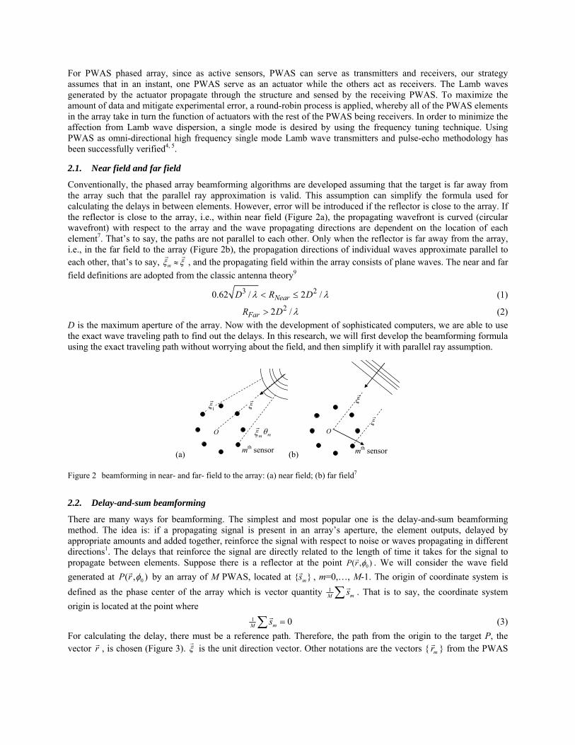
Conventionally, the phased array beamforming algorithms are developed assuming that the target is far away from the array such that the parallel ray approximation is valid. This assumption can simplify the formula used for calculating the delays in between elements. However, error will be introduced if the reflector is close to the array. If the reflector is close to the array, i.e., within near field (Figure 2a), the propagating wavefront is curved (circular wavefront) with respect to the array and the wave propagating directions are dependent on the location of each element7. That’s to say, the paths are not parallel to each other. Only when the reflector is far away from the array, i.e., in the far field to the array (Figure 2b), the propagation directions of individual waves approximate parallel to each other, that’s to say, mξ ξ≈

r r, and the propagating field within the array consists of plane waves. The near and far

field definitions are adopted from the classic antenna theory9

30.62 / 2 /NearD R D2λ λ< ≤ (1)

22 /FarR D λ> (2) D is the maximum aperture of the array. Now with the development of sophisticated computers, we are able to use the exact wave traveling path to find out the delays. In this research, we will first develop the beamforming formula using the exact traveling path without worrying about the field, and then simplify it with parallel ray assumption.

(a)

ξr

1ξr

mξr

mθ

mth sensor

O

(b)

ξr

O ξr

mth sensor

Figure 2 beamforming in near- and far- field to the array: (a) near field; (b) far field7

2.2. Delay-and-sum beamforming

There are many ways for beamforming. The simplest and most popular one is the delay-and-sum beamforming method. The idea is: if a propagating signal is present in an array’s aperture, the element outputs, delayed by appropriate amounts and added together, reinforce the signal with respect to noise or waves propagating in different directions1. The delays that reinforce the signal are directly related to the length of time it takes for the signal to propagate between elements. Suppose there is a reflector at the point 0( , )P r φr . We will consider the wave field generated at 0( , )P r φr by an array of M PWAS, located at { }msr , m=0,…, M-1. The origin of coordinate system is defined as the phase center of the array which is vector quantity 1

mM s∑ r . That is to say, the coordinate system origin is located at the point where 1 0mM s =∑ r (3) For calculating the delay, there must be a reference path. Therefore, the path from the origin to the target P, the vector , is chosen (rr Figure 3). ξ

r is the unit direction vector. Other notations are the vectors { } from the PWAS mr

r

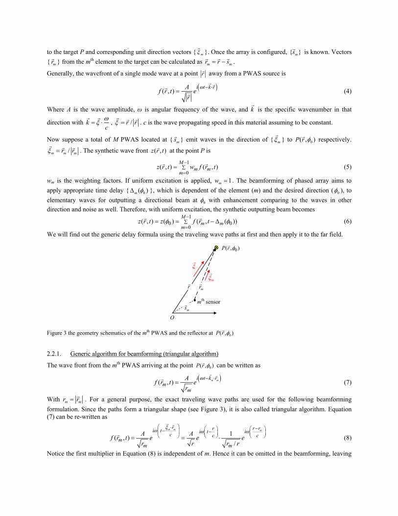
to the target P and corresponding unit direction vectors { mξr

}. Once the array is configured, { }msr is known. Vectors { } from the mmrr th element to the target can be calculated as m mr r s= −

r r r .

Generally, the wavefront of a single mode wave at a point rr away from a PWAS source is

( )( , )i t k rAf r t e

rω − ⋅

=r r

rr (4)

Where A is the wave amplitude, ω is angular frequency of the wave, and kr

is the specific wavenumber in that

direction with kcωξ= ⋅

r r, /r rξ =r r r . c is the wave propagating speed in this material assuming to be constant.

Now suppose a total of M PWAS located at { msr } emit waves in the direction of { mξr

} to 0( , )P r φr respectively.

/m m mr rξ =r r r . The synthetic wave front at the point P is ( , )z r tr

(5) 1

0( , ) ( , )

Mm m

mz r t w f r t∑

−

==

r r

wm is the weighting factors. If uniform excitation is applied, 1mw = . The beamforming of phased array aims to apply appropriate time delay { 0( )m φΔ }, which is dependent of the element (m) and the desired direction ( 0φ ), to elementary waves for outputting a directional beam at 0φ with enhancement comparing to the waves in other direction and noise as well. Therefore, with uniform excitation, the synthetic outputting beam becomes

1

00

( , ) ( ) ( , ( ))M

m mm

z r t z f r t 0φ φ∑−

== = − Δ

r r (6)

We will find out the generic delay formula using the traveling wave paths at first and then apply it to the far field.

0( , )P r φr

rr

msr

mrr

ξr

mξr

O

mth sensor

Figure 3 the geometry schematics of the mth PWAS and the reflector at 0( , )P r φr

2.2.1. Generic algorithm for beamforming (triangular algorithm)

The wave front from the mth PWAS arriving at the point 0( , )P r φr can be written as

( )( , ) m mi t k rm

m

Af r t er

ω − ⋅=

r rr (7)

With m mr r=r . For a general purpose, the exact traveling wave paths are used for the following beamforming

formulation. Since the paths form a triangular shape (see Figure 3), it is also called triangular algorithm. Equation (7) can be re-written as

1( , )/

m m mr r rri t ii tc cc

mm m

A Af r t e e er r r r

ξω ωω⎛ ⎞⋅ −⎛ ⎞⎛ ⎞−⎜ ⎟ −⎜ ⎟ ⎜⎝ ⎠ ⎝ ⎠ ⎝= = ⋅

⎟⎠

r r

r (8)

Notice the first multiplier in Equation (8) is independent of m. Hence it can be omitted in the beamforming, leaving

the 2nd multiplier as the controlling part of beamforming. The synthetic directional signal at direction 0φ therefore is

0( )1

00

1( )/

mm

r riM cm m

z er r

ω φφ

−⎡ ⎤−Δ− ⎢ ⎥⎣ ⎦∑=

= (9)

For the exponential part in the summation, if we have

0( ) mm

r rc

φ−

Δ = (10)

The exponential part will be equal to unit and Equation (9) becomes

1 '

00

1( )/

M

m mz

r rφ

−∑=

= M (11)

Threfore the wave front at 0( , )P r φr is M’ times reinforced with respect to the wave front emitting from the origin.

2.2.2. Far field algorithm for beamforming (parallel algorithm)

As discussed in 2.1, if a reflector is far away from the array, the propagation directions of individual waves can be treated as being parallel to each other, i.e., mξ ξ≈

r r. Therefore for the phase items

m mkc cω ωξ ξ k= ⋅ ≈ ⋅ =

r rr r (12)

For the amplitude items, take the approximation

mr ≈ r (13) With the relationship in Equation (12) and (13), Equation (9) becomes

0( )1

00

( )m

m

siM c

mz e

ξω φφ

⎡ ⎤⋅−Δ⎢ ⎥− ⎣ ⎦∑

==

r r

(14)

If the delays 0( )m φΔ are chosen to be

0( ) mm

sc

ξφ

⋅Δ =

r r

(15)

The output signal at the direction 0φ is

1

00

( ) 1M

mz φ

−∑=

= M (16)

We see that the output signal is M times reinforced with respect to the wave front emitting from the origin and the extent is solely dependent on the number of element in the array. This algorithm is also called parallel algorithm.

3. PWAS PHASED ARRAY DESIGN AND BEAMFORMING SIMULATION The delay formulas developed in previous section is for generic situation, that is to say, effective for any array configuration. Arrays can be arranged in various ways. The simplest array that can be implemented is the linear array by arranging all elements along a straight line. The elements can also be arranged in 2D grid with rectangular shape or circular shape. The design and MathCAD beamforming simulation are dedicated in this section.

3.1. 1D uniformly excited linear PWAS array

Given a linear 1D array consisting of M elements (Figure 4a), elements are equally separated at d. The span D (or the maximum aperture length) of the array is ( 1)D M d≈ − ⋅ (17) Using the concept of phased center, the coordinate system origin is set to be the middle point of the array and the 0° direction coincides with the allignment of the array. Rectangular representation of the location of mth PWAS is

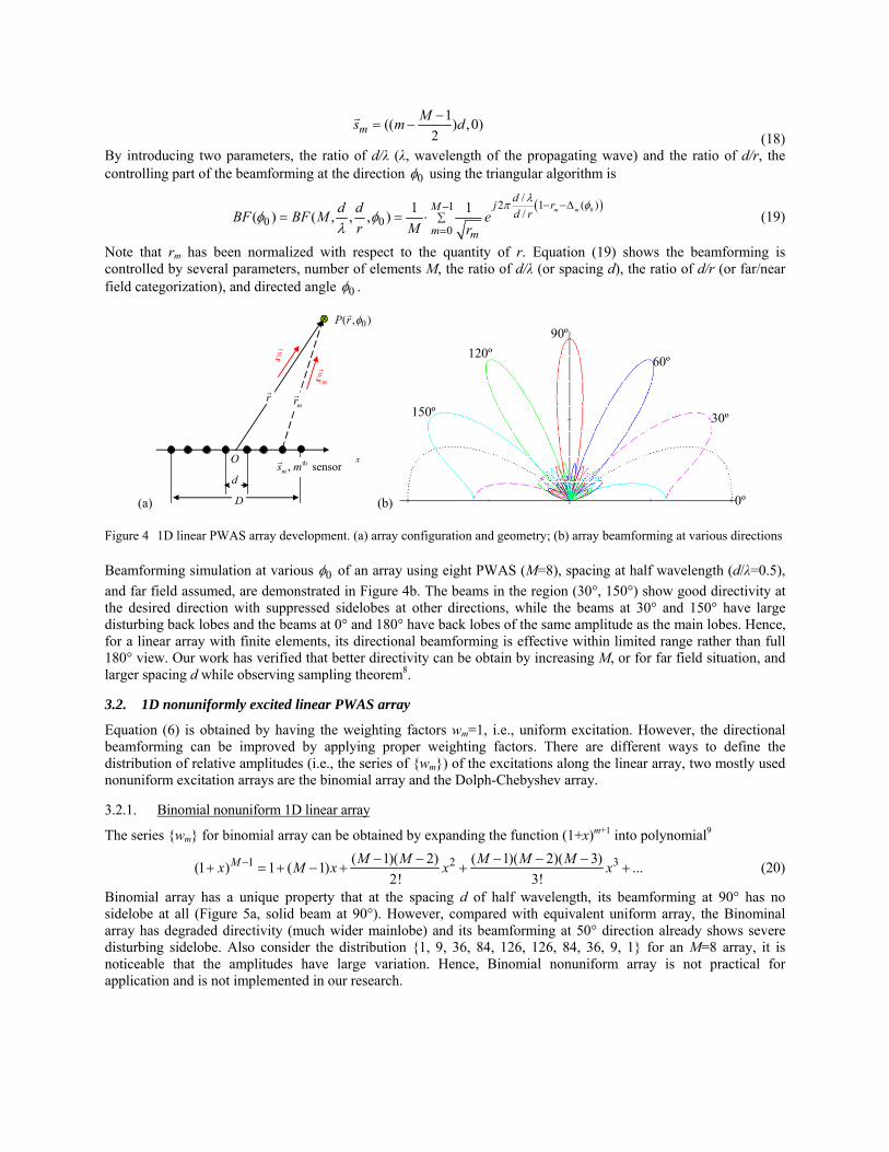
1(( ) ,0)

2mMs m d−

= −r

(18) By introducing two parameters, the ratio of d/λ (λ, wavelength of the propagating wave) and the ratio of d/r, the controlling part of the beamforming at the direction 0φ using the triangular algorithm is

( )0

/2 1 (1 /0 00

1 1( ) ( , , , )m m

dj rM d rm m

d dBF BF M er M r

λπ φφ φ

λ

− −Δ−∑=

= = ⋅)

(19)

Note that rm has been normalized with respect to the quantity of r. Equation (19) shows the beamforming is controlled by several parameters, number of elements M, the ratio of d/λ (or spacing d), the ratio of d/r (or far/near field categorization), and directed angle 0φ .

(a)

0( , )P r φr

rr

th, sensorms mr

mrr

(b)

150º

120º90º

60º

30º

0º

ξr

m

ξr

O

d

D

x

Figure 4 1D linear PWAS array development. (a) array configuration and geometry; (b) array beamforming at various directions

Beamforming simulation at various 0φ of an array using eight PWAS (M=8), spacing at half wavelength (d/λ=0.5), and far field assumed, are demonstrated in Figure 4b. The beams in the region (30°, 150°) show good directivity at the desired direction with suppressed sidelobes at other directions, while the beams at 30° and 150° have large disturbing back lobes and the beams at 0° and 180° have back lobes of the same amplitude as the main lobes. Hence, for a linear array with finite elements, its directional beamforming is effective within limited range rather than full 180° view. Our work has verified that better directivity can be obtain by increasing M, or for far field situation, and larger spacing d while observing sampling theorem8.

3.2. 1D nonuniformly excited linear PWAS array

Equation (6) is obtained by having the weighting factors wm=1, i.e., uniform excitation. However, the directional beamforming can be improved by applying proper weighting factors. There are different ways to define the distribution of relative amplitudes (i.e., the series of {wm}) of the excitations along the linear array, two mostly used nonuniform excitation arrays are the binomial array and the Dolph-Chebyshev array.

3.2.1. Binomial nonuniform 1D linear array

The series {wm} for binomial array can be obtained by expanding the function (1+x)m+1 into polynomial9

1 2( 1)( 2) ( 1)( 2)( 3)(1 ) 1 ( 1) ...2! 3!

M M M M M Mx M x x x− − − − − −+ = + − + + +3 (20)

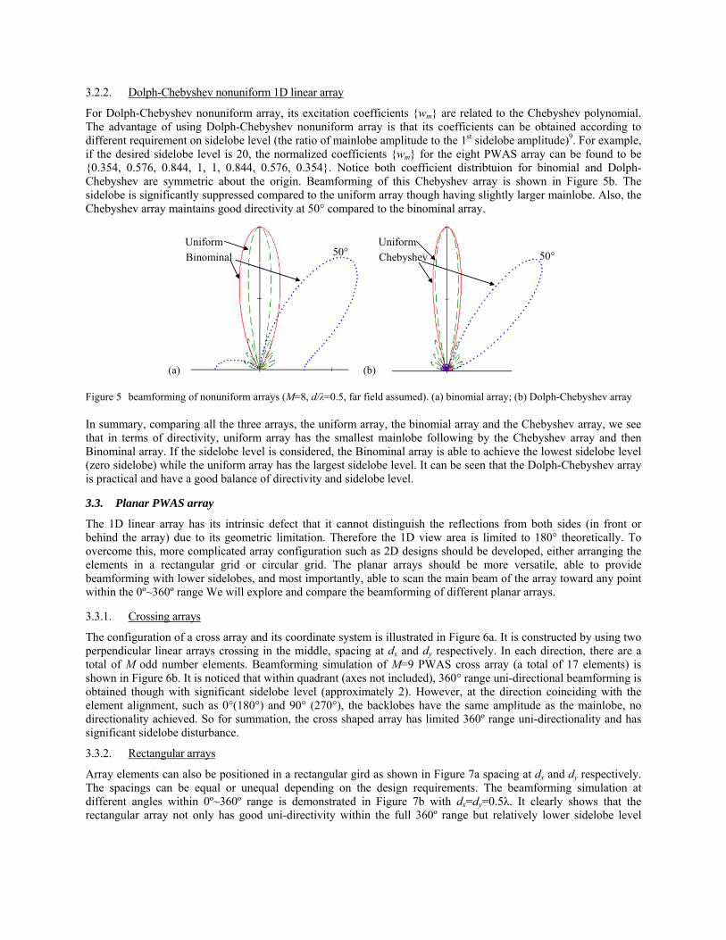
Binomial array has a unique property that at the spacing d of half wavelength, its beamforming at 90° has no sidelobe at all (Figure 5a, solid beam at 90°). However, compared with equivalent uniform array, the Binominal array has degraded directivity (much wider mainlobe) and its beamforming at 50° direction already shows severe disturbing sidelobe. Also consider the distribution {1, 9, 36, 84, 126, 126, 84, 36, 9, 1} for an M=8 array, it is noticeable that the amplitudes have large variation. Hence, Binomial nonuniform array is not practical for application and is not implemented in our research.

3.2.2. Dolph-Chebyshev nonuniform 1D linear array

For Dolph-Chebyshev nonuniform array, its excitation coefficients {wm} are related to the Chebyshev polynomial. The advantage of using Dolph-Chebyshev nonuniform array is that its coefficients can be obtained according to different requirement on sidelobe level (the ratio of mainlobe amplitude to the 1st sidelobe amplitude)9. For example, if the desired sidelobe level is 20, the normalized coefficients {wm} for the eight PWAS array can be found to be {0.354, 0.576, 0.844, 1, 1, 0.844, 0.576, 0.354}. Notice both coefficient distribtuion for binomial and Dolph-Chebyshev are symmetric about the origin. Beamforming of this Chebyshev array is shown in Figure 5b. The sidelobe is significantly suppressed compared to the uniform array though having slightly larger mainlobe. Also, the Chebyshev array maintains good directivity at 50° compared to the binominal array.

(a)

50°Uniform Binominal

(b)

50° UniformChebyshev

Figure 5 beamforming of nonuniform arrays (M=8, d/λ=0.5, far field assumed). (a) binomial array; (b) Dolph-Chebyshev array

In summary, comparing all the three arrays, the uniform array, the binomial array and the Chebyshev array, we see that in terms of directivity, uniform array has the smallest mainlobe following by the Chebyshev array and then Binominal array. If the sidelobe level is considered, the Binominal array is able to achieve the lowest sidelobe level (zero sidelobe) while the uniform array has the largest sidelobe level. It can be seen that the Dolph-Chebyshev array is practical and have a good balance of directivity and sidelobe level.

3.3. Planar PWAS array

The 1D linear array has its intrinsic defect that it cannot distinguish the reflections from both sides (in front or behind the array) due to its geometric limitation. Therefore the 1D view area is limited to 180° theoretically. To overcome this, more complicated array configuration such as 2D designs should be developed, either arranging the elements in a rectangular grid or circular grid. The planar arrays should be more versatile, able to provide beamforming with lower sidelobes, and most importantly, able to scan the main beam of the array toward any point within the 0º~360º range We will explore and compare the beamforming of different planar arrays.

3.3.1. Crossing arrays

The configuration of a cross array and its coordinate system is illustrated in Figure 6a. It is constructed by using two perpendicular linear arrays crossing in the middle, spacing at dx and dy respectively. In each direction, there are a total of M odd number elements. Beamforming simulation of M=9 PWAS cross array (a total of 17 elements) is shown in Figure 6b. It is noticed that within quadrant (axes not included), 360° range uni-directional beamforming is obtained though with significant sidelobe level (approximately 2). However, at the direction coinciding with the element alignment, such as 0°(180°) and 90° (270°), the backlobes have the same amplitude as the mainlobe, no directionality achieved. So for summation, the cross shaped array has limited 360º range uni-directionality and has significant sidelobe disturbance.

3.3.2. Rectangular arrays

Array elements can also be positioned in a rectangular gird as shown in Figure 7a spacing at dx and dy respectively. The spacings can be equal or unequal depending on the design requirements. The beamforming simulation at different angles within 0º~360º range is demonstrated in Figure 7b with dx=dy=0.5λ. It clearly shows that the rectangular array not only has good uni-directivity within the full 360º range but relatively lower sidelobe level

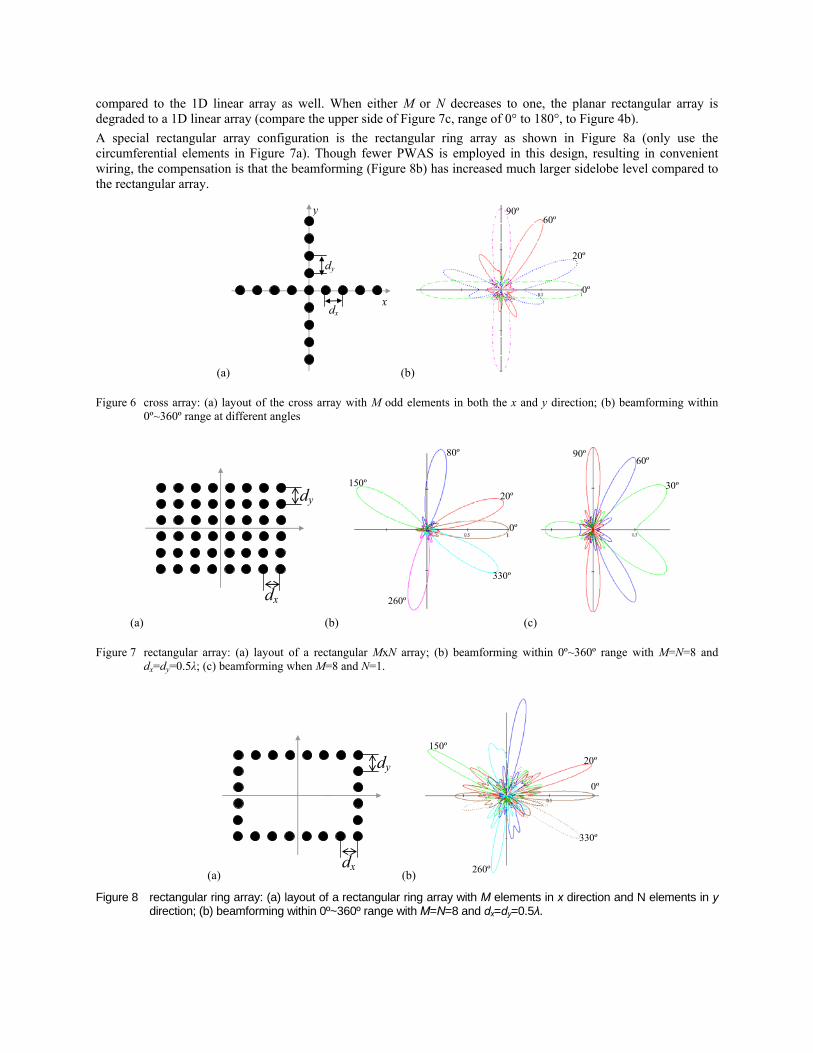
compared to the 1D linear array as well. When either M or N decreases to one, the planar rectangular array is degraded to a 1D linear array (compare the upper side of Figure 7c, range of 0° to 180°, to Figure 4b). A special rectangular array configuration is the rectangular ring array as shown in Figure 8a (only use the circumferential elements in Figure 7a). Though fewer PWAS is employed in this design, resulting in convenient wiring, the compensation is that the beamforming (Figure 8b) has increased much larger sidelobe level compared to the rectangular array.

(a)

dxx

y

dy

(b)

0º

20º

60º 90º

Figure 6 cross array: (a) layout of the cross array with M odd elements in both the x and y direction; (b) beamforming within 0º~360º range at different angles

(a)

dx

dy

(b)

0º

20º

80º

150º

260º

330º

(c)

30º

60º 90º

Figure 7 rectangular array: (a) layout of a rectangular MxN array; (b) beamforming within 0º~360º range with M=N=8 and dx=dy=0.5λ; (c) beamforming when M=8 and N=1.

(a)

dx

dy

(b)

150º

0º

20º

260º

330º

Figure 8 rectangular ring array: (a) layout of a rectangular ring array with M elements in x direction and N elements in y direction; (b) beamforming within 0º~360º range with M=N=8 and dx=dy=0.5λ.

3.3.3. Circular ring array

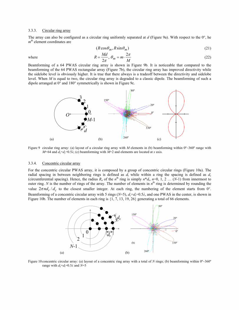
The array can also be configured as a circular ring uniformly separated at d (Figure 9a). With respect to the 0°, he mth element coordinates are ( cos , sin )mR R mθ θ (21)

where 2,

2 mMdR m

Mπθ

π= = ⋅ (22)

Beamforming of a 64 PWAS circular ring array is shown in Figure 9b. It is noticeable that compared to the beamforming of the 64 PWAS rectangular array (Figure 7b), the circular ring array has improved directivity while the sidelobe level is obviously higher. It is true that there always is a tradeoff between the directivity and sidelobe level. When M is equal to two, the circular ring array is degraded to a classic dipole. The beamforming of such a dipole arranged at 0° and 180° symmetrically is shown in Figure 9c.

(a)

0

d

1 2

3

M-1 O

(b)

0º

20º

80º

150º

260º

330º

(c)

Figure 9 circular ring array: (a) layout of a circular ring array with M elements in (b) beamforming within 0º~360º range with M=64 and dx=dy=0.5λ; (c) beamforming with M=2 and elements are located at x axis.

3.3.4. Concentric circular array

For the concentric circular PWAS array, it is composed by a group of concentric circular rings (Figure 10a). The radial spacing in between neighboring rings is defined as dr while within a ring the spacing is defined as dc (circumferential spacing). Hence, the radius Rn of the nth ring is simply n*dr, n=0, 1, 2 … (N-1) from innermost to outer ring. N is the number of rings of the array. The number of elements in nth ring is determined by rounding the value 2 /r cnd dπ to the closest smaller integer. At each ring, the numbering of the element starts from 0°. Beamforming of a concentric circular array with 5 rings (N=5), dc=dr=0.5λ, and one PWAS in the center, is shown in Figure 10b. The number of elements in each ring is {1, 7, 13, 19, 26} generating a total of 66 elements.

(a)

dc

dr0

1 2

N-1 (b)

(b)

0º

20º

80º

150º

260º

330º

Figure 10 concentric circular array: (a) layout of a concentric ring array with a total of N rings; (b) beamforming within 0º~360º range with dc=dr=0.5λ and N=5

Beamforming simulation of such a concentric PWAS array is shown in Figure 10b. Compared with previous achieved beamforming, it has closely the same main lobe width as the rectangular array how a little larger sidelobe level. In terms of implementation, compared to the rectangular array and circular ring array, the installation of concentric array is more difficult to achieve. More experimental research should be conducted regarding the installation concern.

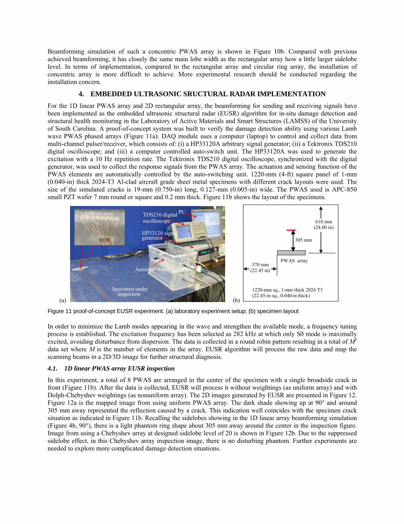
4. EMBEDDED ULTRASONIC SRUCTURAL RADAR IMPLEMENTATION For the 1D linear PWAS array and 2D rectangular array, the beamforming for sending and receiving signals have been implemented as the embedded ultrasonic structural radar (EUSR) algorithm for in-situ damage detection and structural health monitoring in the Laboratory of Active Materials and Smart Structures (LAMSS) of the University of South Carolina. A proof-of-concept system was built to verify the damage detection ability using various Lamb wave PWAS phased arrays (Figure 11a). DAQ module uses a computer (laptop) to control and collect data from multi-channel pulser/receiver, which consists of: (i) a HP33120A arbitrary signal generator; (ii) a Tektronix TDS210 digital oscilloscope; and (iii) a computer controlled auto-switch unit. The HP33120A was used to generate the excitation with a 10 Hz repetition rate. The Tektronix TDS210 digital oscilloscope, synchronized with the digital generator, was used to collect the response signals from the PWAS array. The actuation and sensing function of the PWAS elements are automatically controlled by the auto-switching unit. 1220-mm (4-ft) square panel of 1-mm (0.040-in) thick 2024-T3 Al-clad aircraft grade sheet metal specimens with different crack layouts were used. The size of the simulated cracks is 19-mm (0.750-in) long, 0.127-mm (0.005-in) wide. The PWAS used is APC-850 small PZT wafer 7 mm round or square and 0.2 mm thick. Figure 11b shows the layout of the specimens.

(a)

8 PWAS array

TDS210 digital oscilloscope

HP33120 signalgenerator

Autoswitch unit

Specimen under inspection

PC

(b)

610 mm (24.00 in)

570 mm(22.45 in)

1220-mm sq., 1 - mm thick 2024 T3 (22.45-in sq., 0.040- in thick)

PWAS array

305 mm

Figure 11 proof-of-concept EUSR experiment. (a) laboratory experiment setup; (b) specimen layout

In order to minimize the Lamb modes appearing in the wave and strengthen the available mode, a frequency tuning process is established. The excitation frequency has been selected as 282 kHz at which only S0 mode is maximally excited, avoiding disturbance from dispersion. The data is collected in a round robin pattern resulting in a total of M2 data set where M is the number of elements in the array. EUSR algorithm will process the raw data and map the scanning beams in a 2D/3D image for further structural diagnosis.

4.1. 1D linear PWAS array EUSR inspection

In this experiment, a total of 8 PWAS are arranged in the center of the specimen with a single broadside crack in front (Figure 11b). After the data is collected, EUSR will process it without weightings (as uniform array) and with Dolph-Chebyshev weightings (as nonuniform array). The 2D images generated by EUSR are presented in Figure 12. Figure 12a is the mapped image from using uniform PWAS array. The dark shade showing up at 90° and around 305 mm away represented the reflection caused by a crack. This indication well coincides with the specimen crack situation as indicated in Figure 11b. Recalling the sidelobes showing in the 1D linear array beamforming simulation (Figure 4b, 90°), there is a light phantom ring shape about 305 mm away around the center in the inspection figure. Image from using a Chebyshev array at designed sidelobe level of 20 is shown in Figure 12b. Due to the suppressed sidelobe effect, in this Chebyshev array inspection image, there is no disturbing phantom. Further experiments are needed to explore more complicated damage detection situations.

(a)

(b)

Figure 12 1D linear array EUSR inspection. (a) uniform array; (b) Chebyshev nonuniform array at SLL=20

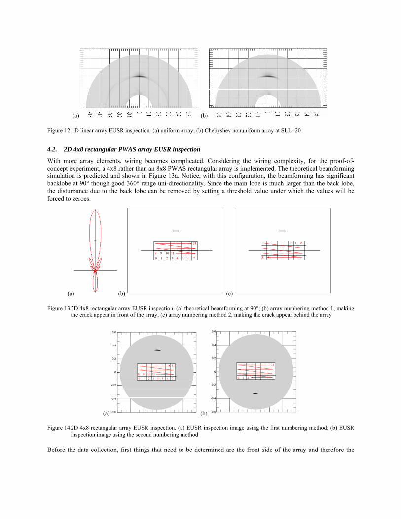
4.2. 2D 4x8 rectangular PWAS array EUSR inspection

With more array elements, wiring becomes complicated. Considering the wiring complexity, for the proof-of-concept experiment, a 4x8 rather than an 8x8 PWAS rectangular array is implemented. The theoretical beamforming simulation is predicted and shown in Figure 13a. Notice, with this configuration, the beamforming has significant backlobe at 90° though good 360° range uni-directionality. Since the main lobe is much larger than the back lobe, the disturbance due to the back lobe can be removed by setting a threshold value under which the values will be forced to zeroes.

(a) (b)

(c)

0 1 2 3 4 5 6 78

31

9 10 11

0 1 2

31

Figure 13 2D 4x8 rectangular array EUSR inspection. (a) theoretical beamforming at 90°; (b) array numbering method 1, making the crack appear in front of the array; (c) array numbering method 2, making the crack appear behind the array

(b)

(a)

0 1 2

31

0 1 2 3 4 5 6 78

31

9 10 11

Figure 14 2D 4x8 rectangular array EUSR inspection. (a) EUSR inspection image using the first numbering method; (b) EUSR inspection image using the second numbering method

Before the data collection, first things that need to be determined are the front side of the array and therefore the

element numbering. The rule of number is to start from the back to front and from left to right. For the 2D PWAS array, it can be numbered in two different ways as demonstrated in Figure 13b and c, resulting different relative angular direction of the crack. For numbering method in Figure 13b, it results in an actual 90° positioned crack, i.e., in front of the array. But for the numbering in Figure 13c, it results in an actual 270° positioned crack, i.e., behind the array. The two different numbering ways are used to demonstrate that our EUSR is able to correctly detect both 90° and 270° defect. Results are shown in Figure 14 after using thresholding to remove the back lobe affection.

5. CONCLUSIONS In this paper, we presented the generic beamforming formulation for PWAS Lamb wave phased array using exact traveling wave paths. The formulas later are simplified with the parallel ray approximation if far field detection is assumed. Using these formulas, beamforming simulation of various array configurations are executed and found that: (1) 1D linear PWAS array has 180° range inspection ability; (b) nonuniformly excited 1D linear PWAS arrays have optimized beamforming compared to uniformly excited array; (3) 2D cross shaped PWAS array has limited 360° range uni-directionality; (4) 2D rectangular and circular shape arrays have good 360° uni-directionality. Proof-of-concept laboratory experiments for using an eight PWAS 1D linear array, uniformly excited and nonuniformly excited (using Dolph-Chebyshev distribution), and using a 4x8 PWAS rectangular 2D array. The using of nonuniformly Dolph-Chebyshev array demonstrated much smaller sidelobe affection. 4x8 PWAS array shows its ability to distinguish a crack from 90° to 270°, having the 360° range detection ability. In order to further confirm the detection ability of the Dolph-Chebyshev array and the 2D array, more complicated damage situation should be explored. Also, the 2D rectangular PWAS array should be experimentally compared to the equivalent circular ring or concentric arrays.

ACKNOWLEDGMENTS This material is based upon work supported by the National Science Foundation under Grant # CMS-0408578 and CMS-0528873, Dr. Shih Chi Liu Program Director and by the Air Force Office of Scientific Research under Grant # FA9550-04-0085, Capt. Clark Allred, PhD Program Manager. Any opinions, findings, and conclusions or recommendations expressed in this material are those of the authors and do not necessarily reflect the views of the National Science Foundation or the Air Force Office of Scientific Research.

REFERENCES 1 Maslak, S. H., “Phased Array Acoustic Imaging System”, U.S. Patent 4,550,607, November 5, 1979 2 Fink, M., “Time Reversal Mirrors”, Journal of Physics D: Applied Physics, Vol. 26, pp. 1333-1350, 1993 3 Deutsch, W.A.K, Cheng, A.; Achenbach, J. D., "Defect Detection with Rayleigh and Lamb Waves Generated

by a Self-Focusing Phased Array", NDT.net, December, Vol. 3 No. 12, March 1998 4 Yu, L. and Giurgiutiu, V., “Improvement of Damage Detection with the Embedded Ultrasonics Structural Radar

for Structural Health Monitoring”, Proceedings of 5th International Workshop on Structural Health Monitoring, Stanford University, Stanford, CA, September 15-17, 2005

5 Bottai, G. and Giurgiutiu, V., “Simulation of the Lamb wave interaction between piezoelectric wafer active sensors and host structure”, Proceedings of SPIE Smart Structures and Materials 2005, May 2005, pp. 259-270

6 Krautkramer, J.; Krautkramer, H. Ultrasonic Testing of Materials, Springer-Verlag, 1990 7 Johnson, D.H. and Dudgeon, D.E. (1993), Array Signal Processing, Prentice Hall PTR, Upper Saddle River, NJ

07458 8 Yu, L. and Giurgiutiu, V. (2005), “Using Phased Array Technology And Embedded Ultrasonic Structural Radar

For Active Structural Health Monitoring And Nondestructive Evaluation”, Proceedings of 2005 ASME International Mechanical Engineering Congress, November 5-13, Orlando, FL, paper # IMECE2005-80227

9 Balanis, C.A. (2005) , Antenna Theory, John Wiley & Sons, Inc., Hoboken, NJ 07030