Design, Fabrication And Testing Of A Low Temperature Heat ...
165
University of Central Florida University of Central Florida STARS STARS Electronic Theses and Dissertations, 2004-2019 2009 Design, Fabrication And Testing Of A Low Temperature Heat Pipe Design, Fabrication And Testing Of A Low Temperature Heat Pipe Thermal Switch With Shape Memory Helical Actuators Thermal Switch With Shape Memory Helical Actuators Othmane Benafan University of Central Florida Part of the Engineering Commons Find similar works at: https://stars.library.ucf.edu/etd University of Central Florida Libraries http://library.ucf.edu This Masters Thesis (Open Access) is brought to you for free and open access by STARS. It has been accepted for inclusion in Electronic Theses and Dissertations, 2004-2019 by an authorized administrator of STARS. For more information, please contact [email protected]. STARS Citation STARS Citation Benafan, Othmane, "Design, Fabrication And Testing Of A Low Temperature Heat Pipe Thermal Switch With Shape Memory Helical Actuators" (2009). Electronic Theses and Dissertations, 2004-2019. 1508. https://stars.library.ucf.edu/etd/1508
Transcript of Design, Fabrication And Testing Of A Low Temperature Heat ...

University of Central Florida University of Central Florida
STARS STARS
Electronic Theses and Dissertations, 2004-2019
2009
Design, Fabrication And Testing Of A Low Temperature Heat Pipe Design, Fabrication And Testing Of A Low Temperature Heat Pipe
Thermal Switch With Shape Memory Helical Actuators Thermal Switch With Shape Memory Helical Actuators
Othmane Benafan University of Central Florida
Part of the Engineering Commons
Find similar works at: https://stars.library.ucf.edu/etd
University of Central Florida Libraries http://library.ucf.edu
This Masters Thesis (Open Access) is brought to you for free and open access by STARS. It has been accepted for
inclusion in Electronic Theses and Dissertations, 2004-2019 by an authorized administrator of STARS. For more
information, please contact [email protected].
STARS Citation STARS Citation Benafan, Othmane, "Design, Fabrication And Testing Of A Low Temperature Heat Pipe Thermal Switch With Shape Memory Helical Actuators" (2009). Electronic Theses and Dissertations, 2004-2019. 1508. https://stars.library.ucf.edu/etd/1508

i
DESIGN, FABRICATION AND TESTING OF A LOW TEMPERATURE HEAT PIPE THERMAL SWITCH WITH
SHAPE MEMORY HELICAL ACTUATORS
by
OTHMANE BENAFAN B.S. University of Central Florida, 2008
A thesis submitted in partial fulfillment of the requirements for the degree of Master of Science
in the Department of Mechanical, Materials and Aerospace Engineering in the College of Engineering and Computer Science
at the University of Central Florida Orlando, Florida
Summer Term 2009

ii
© 2009 Othmane Benafan

iii
ABSTRACT
This work reports on the design, fabrication and testing of a thermal switch wherein the
open and closed states are actuated by shape memory alloy elements while heat is transferred by
a heat-pipe. The motivation for such a switch comes from NASA's need for thermal management
in advanced spaceport applications associated with future lunar and Mars missions. For example,
as the temperature can approximately vary between 40 K to 400 K during lunar day/night cycles,
such a switch can reject heat from a cryogen tank in to space during the night cycle while
providing thermal isolation during the day cycle. By utilizing shape memory alloy elements in
the thermal switch, the need for complicated sensors and active control systems are eliminated
while offering superior thermal isolation in the open state. Nickel-Titanium-Iron (Ni-Ti-Fe)
shape memory springs are used as the sensing and actuating elements. Iron (Fe) lowers the phase
transformation temperatures to cryogenic regimes of operation while introducing an
intermediate, low hysteretic, trigonal R-phase in addition to the usual cubic and monoclinic
phases typically observed in binary NiTi. The R-phase to cubic phase transformation is used in
this application. The methodology of shape memory spring design and fabrication from wire
including shape setting is described. Heat transfer is accomplished via heat acquisition, transport
and rejection in a variable length heat pipe with pentane and R-134a as working fluids. The
approach used to design the shape memory elements, quantify the heat transfer at both ends of
the heat pipe and the pressures and stresses associated with the actuation are outlined. Testing of
the switch is accomplished in a vacuum bell jar with instrumentation feedthroughs using valves
to control the flow of liquid nitrogen and heaters to simulate the temperature changes. Various

iv
performance parameters are measured and reported under both transient and steady-state
conditions. Funding from NASA Kennedy Space Center for this work is gratefully
acknowledged.

v
Dedicated
to my Parents
vi
ACKNOWLEDGMENTS
First and foremost, I would like to express my sincere gratitude to my advisor Dr. Raj
Vaidyanathan for introducing me to graduate research and giving me the opportunity to pursue a
Masters degree in Mechanical Engineering, and for his valuable advice and guidance throughout
my thesis project and research. My gratitude also goes out to Dr. William U. Notardonato
(NASA-KSC) and Dr. Barry J. Meneghelli (ASRC) for involving me in developing a shape
memory alloy thermal switch for NASA‟s thermal management.
I would like to thank Dr. Ali P. Gordon, Dr. Jayanta Kapat and Dr. William U.
Notardonato for their valuable advice and for serving on my defense committee. I would also
like to thank my office friends and colleagues Shipeng Qiu, R. Mahadevan Manjeri, Matthew D.
Fox and Vinu B. Krishnan for responding to my never ending questions and sharing their
knowledge in shape memory alloys with me. My sincere gratitude is also extended to the AMPAC
administrative staff, Ms. Angelina Feliciano, Ms. Cynthia Harle, Ms. Karen Glidewell, and Ms.
Kari Stiles for dealing with all the paperwork and ordering project and lab materials. I also thank
Richard E. Zotti of CREOL and Mark D. Velasco of ASRC for their contributions in parts
machining and helpful suggestions.
Above all I would like to thank all my friends, my sisters Rabia, Naima, Souad and
Kaoutar, my brother Hicham, and Eunice who have advised and encouraged me to sail through
this journey at UCF. Finally I humbly thank and dedicate this work to my parents, Mueha and
Buiga, for their boundless love and support, and for their guidance not only in this work but also
in everyday decisions.

vii
TABLE OF CONTENTS
LIST OF FIGURES……………………………………………..........................................……...x
LIST OF TABLES………………………………………………..........................................…...xv
LIST OF ACRONYMS/ABBREVIATIONS……...……………..........................................…..xvi
CHAPTER ONE: INTRODUCTION……………………………………......................................1
1.1 Motivation...……………………………………………………………………….....1
1.2 Organization………………………………………………………………...……..…4
CHAPTER TWO: LITERATURE REVIEW………………………………………………..........5
2.1 Shape Memory Alloys………………………………...……………………..…….....5
2.1.1 Shape Memory Effect………....……………………………………………6
2.1.2 Superelasticity…………………………………………………………...…9
2.2 Applications of Shape Memory Alloys….………………………..………………...10
2.3 The R-Phase in NiTi System………………………………………………………..12
2.4 Thermal Switches…………………………………………………………………...13
CHAPTER THREE: NiTiFe SHAPE MEMORY ALLOY HELICAL ACTUATORS………...17
3.1 Helical Spring Analyses……………………………………………………………...17
3.2 Helical Shape Memory Alloy Actuators ………………..……………...……………19
3.3 Helical Shape Memory Alloy Actuator Design……………….……...……………...20
3.3.1 Equations in Reduced Form….…..….……..……………………………..23
3.3.2 Equations in Full Form….……...………….……………………………...26
3.3.3 Finite Element Method…...…….…………………………………………27
viii
3.3.4 Comparisons Between Elastic Theory and the Finite Element Method..29
3.4 Fabrication of Actuators …………...…………………..…………………..……38
3.5 Thermal Switch Actuation…………..……………………………………...……42
CHAPTER FOUR: VARIABLE LENGHT TWO-PHASE HEAT PIPE ……..……………......44
4.1 Overview…………………………….…………………………...…………………44
4.2 Closed Two-Phase Thermosyphon Design……....……………………………...….47
4.2.1 Heat Transfer at the Evaporator………………….…………………….....47
4.2.2 Heat Transfer at the Condenser…….…………………………………..…50
4.2.3 Limitations of Two-Phase Thermosyphon ……………………...………..52
4.3 Heat Pipe Fabrication and Assembly ………………………...…………………….53
4.4 Thermophysical Properties of the Working Fluids …………………….…………..55
CHAPTER FIVE: THERMAL SWITCH ASSEMBLY AND OPERATION………………......57
5.1 Thermal Switch Components and Final Assembly……..….……………………....57
5.2 Switch Opeartion…………………...……………………………………………....60
CHAPTER SIX: TEST SETUP AND METHODOLOGY……………………...……………....62
6.1 Heat Pipe Evacuation and Charging………..…….….…………..……….…….......62
6.2 Thermal Switch Test Setup……………….…………………………………...……64
6.3 Testing Methodology………………………………………………….……………71
6.4 Instrumentation and LabVIEW® Data Acquisition…….………...……………...…72
6.4.1 Temperature Virtual Instrument…………………………………………..73
6.4.2 Displacement Virtual Instrument……..……….....….…..………...……...75
6.4.3 Load Virtual Instrument…………………………….………………...…..77
ix
CHAPTER SEVEN: RESULTS AND DISCUSSION………..................................................…79
7.1 Differential Scanning Calorimetry………..………………...……………..……......79
7.2 SMA Actuators Temperature Distribution………………...……………………..…82
7.3 Performance of the Shape Memory Helical Actuators ……………………….……84
7.4 Performance of the Thermal Switch…….........…………..……………………...…91
CHAPTER EIGHT: CONCLUSIONS AND FUTURE WORK…………………………...........99
8.1 Conclusions……...………………..………...……………...…………………........99
8.2 Future Work and Recommendations……...…...………………………………….100
APPENDIX A: DESIGN CALCULATIONS…………………………………………..…....102
A-1 Spring Design Equations and Calculations…………………..……………………103
A-2 Comparison of SMA Spring Design Equations…………………………………...108
A-3 Heat Pipe Internal Stress Analysis Equations……...……………………………...110
A-4 Heat Transfer Design Equations and Calculations (for R-134a)………………….111
A-5 Heat Transfer Design Equations and Calculations (for Pentane)…...…………….116
A-6 Liquid Pool Calculations (with Pentane): Film Thickness Calculation…………...120
APPENDIX B: DESIGN DRAWINGS…………………………………………………..….....124
REFERENCES…………………………………………………………………………………143

x
LIST OF FIGURES
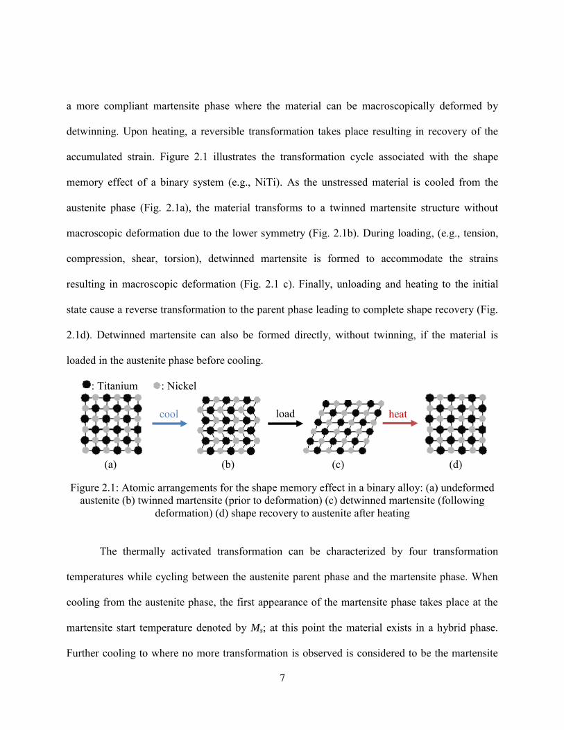
Figure 2.1: Atomic arrangements for the shape memory effect of a binary alloy: (a) undeformed austenite (b) twinned martensite (prior to deformation) (c) detwinned martensite (following deformation) (d) shape recovery to austenite after heating…………………………………………………………………………….7
Figure 2.2: Transformation temperatures and hysteresis associated with the shape memory effect…………………………………………………………………………...….8
Figure 2.3: Superelasticity: (a) austenite (b) stress-induced martensite (c) shape recovery on reverse transformation to austenite…………………………………………….....9
Figure 2.4: Superelastic behavior during loading and unloading at constant temperature: ABC during loading resulting in the forward phase transformation; DEF during unloading resulting in the reverse transformation…………………………….....10
Figure 2.5: Shape memory alloy actuated variable geometry chevrons [26]………………..11
Figure 2.6: Example of a differential thermal expansion thermal switch. (a) open-state at high temperature (b) closed-state at low temperature [31]…………………………....14
Figure 2.7: Example of a gas-gap thermal switch with an adsorption pump [32]……….…..15
Figure 2.8: Example of a sealed bellows thermal switch [33]………………………...…..…16
Figure 3.1: SMA helical spring length: (a) high temperature phase (b) low temperature phase………………………………………………………………………….….20
Figure 3.2: Global and local reference coordinate systems for the spring……………..……21
Figure 3.3: Free body diagram (a) resultant moment (b) resultant force………………….…21
Figure 3.4: Finite element mesh used to model spring……………………………………....28
Figure 3.5: Shear stress distribution across coil section in a helical SMA spring: (a) FEA (b) prediction from theory (spring axis to the right)………………………………...30
Figure 3.6: z shear stress distribution for a spring cross-section with small helix angle ≈
2° (austenite, spring axis to the right)…………………………………………...31
Figure 3.7: Comparison of maximum shear stress (z) using elastic theory and FEA (austenite)………………………………………………………………………..32
xi
Figure 3.8: z distribution for F= 9 N in helical coil (austenite)…………………………….33
Figure 3.9: z as a function of helical angle for various loads (austenite)………………..…34
Figure 3.10: Spring displacement in tension for small helix angle ≈ 2° (austenite, bottom of spring fixed and load applied at the top end)…………………………………....35
Figure 3.11: Correlation between spring extension and helical angle (austenite)…………….36
Figure 3.12: Correlation between spring extension and helical angle (R-phase)……………..37 .
Figure 3.13: Helical shape memory alloy actuators and spring winding mandrels………..….38
Figure 3.14: Mandrel containing coiled SMA wire in the furnace……………………………39
Figure 3.15: Spring geometry 3 after shape setting and final electrical discharge machining to increase contact………………………………………………………………….40
Figure 3.16: Load-extension response of the SMA springs at room temperature………...…..41
Figure 3.17: Arrangement of the shape memory (dark shading) and bias springs (light shading) (a) at high temperature with the SMA spring pre-loaded and the bias spring compressed in the open or “off” position; and (b) at low temperature with the
SMA spring extended and the bias spring in the closed or “on” position (c)
Sectional view of the shape memory and bias springs…………………………..43
Figure 3.18: Arrangement of the shape memory (dark shading) and bias springs (light shading) in the switch (a) at high temperature with the SMA spring pre-loaded and the bias spring compressed in the open or “off” position; and (b) at low temperature with
the SMA spring extended and the bias spring in the closed or “on” position…...43
Figure 4.1: Sections in a heat pipe involving two-phase flow…………………………….…45
Figure 4.2: Critical regions in a pool boiling curve [70]………………………………….....48
Figure 4.3: Assembly of the closed two-phase thermosyphon: (a) schematic, with the regions A, B, and C being the condensation, adiabatic, and evaporation regions, respectively (b) final assembly…………………………………………………..54
Figure 5.1: Schematic of final thermal switch assembly (dimensions in mm)………………58

xii
Figure 5.2: Final thermal switch assembly. The bias spring in the front was removed to show the position of the SMA spring……………………………………………...…..59
Figure 5.3: Principle of switch operation: (a) The open or “off” position during a lunar day
(hot) (b) and the closed or “on” position during a lunar night (cold)………..….61
Figure 6.1: Pressure manifold for heat pipe evacuation and charging…….………………....63
Figure 6.2: Heat pipe evacuation /charging setup…………………………………………....64
Figure 6.3: Test stand with thermal switch: (a) schematic (b) final setup………………..….65
Figure 6.4: Single-loop cooper tube around thermal switch………………………………....66
Figure 6.5: Fabrication of the single-loop copper tube………………………………………66
Figure 6.6: Glass bell jar with instrumentation feedthroughs………………………………..69
Figure 6.7: Thermal switch inside the bell jar fixture………………………………………..70
Figure 6.8: Thermal switch and single-loop cooling coils connected to liquid nitrogen lines……………………………………………………………………………...70
Figure 6.9: Switch in instrumented vacuum bell jar setup for testing. LabVIEW® software was used for data acquisition and control of the test temperature conditions (heater and flowing liquid nitrogen through coils)…………………………..…..71
Figure 6.10: LabVIEW ® data acquisition system…………………………………………….72
Figure 6.11a: Virtual instrument block diagram for temperature measurement…………….…73
Figure 6.11b Virtual instrument front panel for temperature measurement……………….…..74
Figure 6.12a: Virtual instrument block diagram for displacement measurement………...……75
Figure 6.12b: Virtual instrument front panel for displacement measurement……………….....76
Figure 6.13a: Virtual instrument block diagram for acquiring load cell data (NI code)……….77
Figure 6.13b: Virtual instrument front panel for acquiring load cell data (NI code)…………..78
Figure 7.1: Differential Scanning Calorimetry curves of the shape set NiTiFe wire………..80
Figure 7.2: DSC response of NiTiFe in the as-received, shape set and tested conditions…...81

xiii
Figure 7.3: Cooling and heating rates of the four SMA helical springs……………………..82
Figure 7.4: Temperature distribution along the length of the SMA spring……………….....83
Figure 7.5: Experimental and theoretical load-extension response of the springs in the austenite and R-phase and the bias springs…………………………………..….84
Figure 7.6: Stroke-temperature response of the shape memory helical actuators. The transformation temperatures Rf, Rs, As, and Af under the bias load are -15.2, -75.5, -61.3 and 3.1 ± 2 oC respectively……………………………………….…86
Figure 7.7: Stroke-time response of the shape memory helical actuators to assess open-loop strains. After the third cycle from room temperature to -100 oC at 10oC/min, the open loop axial deformation is negligible as shown by 3 for an overall switch extension of 5 mm…………………………………………………………….....86
Figure 7.8: Stroke-temperature response of the shape memory helical actuators under varying bias loads. Fb denotes the total bias force from stainless steels springs, bellows and weight of the heat pipe. The maximum stroke for (a), (b), (c), and (d) are 1.85, 2.94, 5.0, and 7.13 mm, respectively. The graphs y-axes are scaled identically………………………………………………………………………..87
Figure 7.9: Stroke-time response of the shape memory helical actuators under varying bias loads. Fb denotes the total bias force from stainless steels springs, bellows and weight of the heat pipe. The graphs y-axes are scaled identically.…………...…88
Figure 7.10: Shear stress evolution with temperature in a spring during 5 mm extension against a total bias load of 39 N…………………………………………...…….89
Figure 7.11: Effect of load on transformation temperatures………………………….…...…..90
Figure 7.12: Heat transfer rate as a function of contact pressure……………………………..92
Figure 7.13: Contact force with switch extension. The minimum required contact force is from Fig. 7.12………………………………………………………………………….92
Figure 7.14: Baseline test with no working fluid (conduction only). An average heat transfer rate of 3.6 W was obtained………………………………………………………94
Figure 7.15: Heat throughput using pentane: (a) F.R. = 0.5, Q = 8.6 W (b) F.R. = 0.7, Q = 11.3 W (c) F.R. = 0.9, Q = 12.9 W (d) F.R. = 1.5, Q = 7.1 W………………………..95
Figure 7.16: Heat throughput using pentane: (a) F.R. = 0.5, Q = 7.1 W (b) F.R. = 0.7, Q = 9.1 W (c) F.R. = 0.9, Q = 10.2 W (d) F.R. = 1.5, Q = 5.8 W……………………......96

xiv
Figure 7.17: Heat transfer rate with fill ratio, with pentane and R-134a as working fluids in the
heat pipe. Lf is the liquid pool length and Le is the length of the evaporator....…97
Figure 7.18: Average heat transfer rate using pentane……………………………………..…98
Figure 7.19: Average heat transfer rate using R-134a…………………………………….......98

xv
LIST OF TABLES
Table 3.1: Mechanical properties of NiTiFe used in the analytical and FEM models …….....28
Table 3.2: NiTiFe Spring dimensions used in the analytical and FEM models………………28
Table 3.3: Shape memory alloy spring geometries (wire diameter 2.159 mm)………………40
Table 3.4: Shape memory alloy spring constants (wire diameter 2.159 mm)……………...…40
Table 4.1: Thermophysical saturation properties for pentane (liquid phase)………….……...55
Table 4.2: Thermophysical saturation properties for pentane (vapor phase)………………....56
Table 4.3: Thermophysical saturation properties for R-134a (liquid phase)…………….…....56
Table 4.4: Thermophysical saturation properties for R-134a (vapor phase)……………..…...56
Table 7.1: Transformation temperatures of NiTiFe in the as-received, shape set and tested conditions…………………………………………………...…………………….81

xvi
LIST OF ACRONYMS/ABBREVIATIONS
Af Austenite finish
As Austenite start
CTPT Closed Two-Phase Thermosyphon
DSC Differential Scanning Calorimetry
EDM Electrical-Discharge Machining
F.R. Fill Ratio
KSC Kennedy Space Center
LOX Liquid Oxygen
Mf Martensite finish
Ms Martensite start
NASA National Aeronautics and Space Administration
NI National Instruments
NiTi Nickel-Titanium (alloy)
NiTiFe Nickel Titanium Iron (alloy)
Rf R-phase finish
R-phase Rhombohedral-phase
Rs R-phase start
SE Superelasticity
SMA Shape Memory Alloy
SME Shape Memory Effect
1
CHAPTER ONE: INTRODUCTION
1.1 Motivation
The need for thermal management in both ground and space-based aerospace applications
has gained greater interest in the last decade. Earth orbiting spacecrafts and future outposts on
the moon and Mars contain structures that require effective thermal control. Heat exchangers
and other heat rejection systems are currently used in high temperature applications, but thermal
solutions are limited in the low temperature regime where there are specific needs, e.g., to
minimize or eliminate cryogen boil-off and parasitic heat loads, to transfer heat on-demand in
cases where there are restrictions on the number of chillers or coolers, etc., among others.
Among many devices used to solve these problems, thermal switches have been at the forefront.
Gas-gap, paraffin, and differential thermal expansion thermal switches have been developed and
used [1-4]; however, these devices usually require external sensors, electric heaters or pumps,
and do not integrate sensor and actuator capability in a single mechanism. Shape memory alloys
(SMAs) are materials that integrate both sensory and actuation functions due to a temperature-
induced solid-state phase transformation that can bring about shape changes against external
loads. These “smart” alloys recover considerable inelastic distortion (up to 8% strain) against
large stresses (up to 500 MPa) associated with the shape memory effect (SME) and pseudo-
elasticity (stress removal recovery) [5-10]. Among many classes of shape memory alloys, near
equi-atomic NiTi is a commonly used SMA owing to its favorable mechanical properties [11],
but devices that incorporate binary NiTi are limited to operating near room temperature. The
2
transformation in NiTi occurs between a higher temperature cubic phase called austenite phase
and a lower temperature monoclinic phase called martensite phase and has a hysteresis
associated with it. Addition of a third element such as iron (Fe) introduces a stable intermediate
trigonal R-phase with improved fatigue response and reduced hysteresis while suppressing the
phase transformation and shifting it to lower temperatures [12-17]. Strains associated with the R-
phase are typically limited to about 1% and hence helical spring SMA elements are used in this
work to attain large strokes and adequate work output. Helical actuators provide greater strokes
and uniform stress distribution when compared to other element forms such as strips (e.g., Ref.
[18]). In addition, these novel actuators are lightweight and compact in size compared to the
conventional actuators such as electric motors, hydraulic cylinders, or pneumatic actuators. SMA
helical actuators have further advantages in space applications; for instance, they operate in a
spark-free way avoiding any faulting or ignition of electrical components that can interrupt the
continuity of operation.
Previously, low temperature shape memory alloy thermal switches were developed and
tested at the University of Central Florida (UCF) based on conduction [18, 19]. These conduction
switches were designed for use in space applications for zero boil-off control, heat transfer
between two cryogenic storage tanks and parasitic heat load reduction from secondary redundant
cryocoolers. Use of a variable length, two-phase heat pipe promotes heat acquisition, transport
and rejection via evaporation and condensation in addition to conduction. Two-phase heat pipes
are advantageous in that they offer enhanced heat transfer and allow reductions in component
weight and volume without decreasing performance. Furthermore, two-phase heat pipes are self-
contained without any pumping mechanism thereby eliminating the need for external pumps.

3
Since heat pipes do not require large contact areas for efficient heat transfer, parasitic heat loads
are minimized due to complete thermal isolation and low surface radiation in the open or “off”
position.
Thus the objective of this work is to combine low temperature helical SMA actuators
with a variable length, two-phase heat pipe in a thermal switch to meet NASA‟s thermal
management needs. A heat pipe incorporated in such switches can provide heat transfer
involving two-phase flow via evaporation and condensation of the working fluid. The ability of
the switch to alternate between the closed or “on” and the open or “off” states without external
sensors and mechanisms potentially finds direct applications in advanced spaceport technologies
associated with future lunar and Mars missions. The proposed passive control SMA thermal
switch eliminates the need for external mechanical means for actuation or pumping fluid making
it an efficient device and a less complicated system to integrate in space structures.
Procedures related to the design, construction, combination of parts and final assembly
are presented. Experiments were done to quantitatively obtain performance parameters such as
deflection curves, force output, and heat transfer rates. Data was collected while testing under
vacuum conditions in a sealed glass bell jar with multiple instrumentation feedthroughs for
thermocouples, the load cell, the linear encoder, heating pads, liquid nitrogen flow, vacuum
valves, and the viewing port. LabVIEW® was used for data acquisition and control of the test
temperature conditions. Experimental results were compared with analytical and computational
results where possible.

4
1.2 Organization
The work presented is subdivided into chapters organized as follows: Chapter 2 is an
introduction to shape memory alloys along with their applications. A brief introduction to
thermal switches and their operation is also presented. Chapter 3 presents the design and
fabrication of the low temperature shape memory alloy helical actuators used based on spring
theories and the finite element method. Chapter 4 presents the design methodology and
fabrication of a gravity-assisted two-phase heat pipe. The approach used to quantify the heat
transfer rate at both ends of the pipe is outlined. Chapter 5 describes the final switch assembly
and operation. Chapter 6 gives a brief overview of the test setup, instrumentation and procedures
used to quantify the thermal switch performance parameters. Chapter 7 presents results and
discusses material characterization, helical actuators performance and heat transfer aspects.
Finally, Chapter 8 presents conclusions and recommendations. Relevant design calculations and
machine drawings are included in the Appendix.

5
CHAPTER TWO: LITERATURE REVIEW
Shape memory alloys have received considerable interest in the last two decades due to
their favorable thermo-mechanical characteristics, leading to their use in various applications
ranging from medical to aerospace industries. Among many classes of shape memory alloys,
binary nickel-titanium alloys exhibiting both shape memory and superelastic behavior are
commonly used. This chapter describes the phase transformation in NiTi alloys and metallurgical
aspects. Use of an intermediate R-phase for actuation at low temperatures as a result of element
addition is described. An introduction to thermal switches and their applications is outlined in the
last section of this chapter.
2.1 Shape Memory Alloys
Shape memory alloys are novel materials that remember their pre-deformed shape by
undergoing a reversible solid-state phase transformation induced by changes in temperature
and/or stress. This phase change is first-order and is characterized by no change in chemical
composition or atomic diffusion, and takes place in the form of shearing deformation of the
crystallographic structure between a low-symmetry so-called martensite phase and a high-
symmetry so-called austenite parent phase. Depending on stoichiometry, the austenitic phase has
a cubic (B2) structure and it is usually associated with high-temperatures; alternatively, the
martensitic phase has a monoclinic (B19') structure and is associated with low-temperatures.
Shape memory alloys can recover considerable inelastic deformation (up to 8% uniaxial strain)
against large stresses (up to 500 MPa) which gives them the ability to be used as actuators [11].
6
Among many classes of SMAs, NiTi alloys and copper based alloys have been at the forefront due
to large stain recovery coupled with superior force generation when compared to other alloy systems.
Observations of SMA behavior were first investigated and discovered in 1932 in Au-Cd system
by Arne Ӧlander [20]. In 1938, Greninger and Mooradian observed the shape memory effect in
copper-zinc (Cu-Zn) and copper-tin (Cu-Sn) alloys [21]. Around 30 years later in 1962, such
behavior was discovered in nickel-titanium (NiTi) in several studies conducted at the U.S. Naval
Ordnance Laboratories [22]. Since then, extensive research has been devoted to better understand
the physical and mechanical properties of these materials.
The shape change in SMAs results from thermal or stress induced transformation.
Thermally induced phase transformation, resulting in the shape memory effect (SME), occurs by
cycling the material between high and low temperatures with or without a pre-stress. As the
material transforms back from low to high temperature, the martensite phase becomes unstable
and transforms back to the parent phase (austenite) recovering all the macroscopic strains. The
stress-induced transformation, resulting in superelasticity (SE), occurs by loading the material in
its austenite phase to form stress-induced martensite (SIM). Upon unloading, the material goes
back to its original shape without permanent plastic deformation. Details of these two behaviors
are discussed in the next sections.
2.1.1 Shape Memory Effect
The shape memory effect refers to the ability of the alloy to recover or “remember” its
original shape by increasing the temperature while in its low temperature phase. When cooling
from the stiffer austenite phase, the material undergoes a displacive martensitic transformation to
7
a more compliant martensite phase where the material can be macroscopically deformed by
detwinning. Upon heating, a reversible transformation takes place resulting in recovery of the
accumulated strain. Figure 2.1 illustrates the transformation cycle associated with the shape
memory effect of a binary system (e.g., NiTi). As the unstressed material is cooled from the
austenite phase (Fig. 2.1a), the material transforms to a twinned martensite structure without
macroscopic deformation due to the lower symmetry (Fig. 2.1b). During loading, (e.g., tension,
compression, shear, torsion), detwinned martensite is formed to accommodate the strains
resulting in macroscopic deformation (Fig. 2.1 c). Finally, unloading and heating to the initial
state cause a reverse transformation to the parent phase leading to complete shape recovery (Fig.
2.1d). Detwinned martensite can also be formed directly, without twinning, if the material is
loaded in the austenite phase before cooling.
: Titanium : Nickel
Figure 2.1: Atomic arrangements for the shape memory effect in a binary alloy: (a) undeformed
austenite (b) twinned martensite (prior to deformation) (c) detwinned martensite (following deformation) (d) shape recovery to austenite after heating
The thermally activated transformation can be characterized by four transformation
temperatures while cycling between the austenite parent phase and the martensite phase. When
cooling from the austenite phase, the first appearance of the martensite phase takes place at the
martensite start temperature denoted by Ms; at this point the material exists in a hybrid phase.
Further cooling to where no more transformation is observed is considered to be the martensite
load
(
a)
(
d)
(
c)
(
b)
cool heat
(a) (b) (c) (d)
8
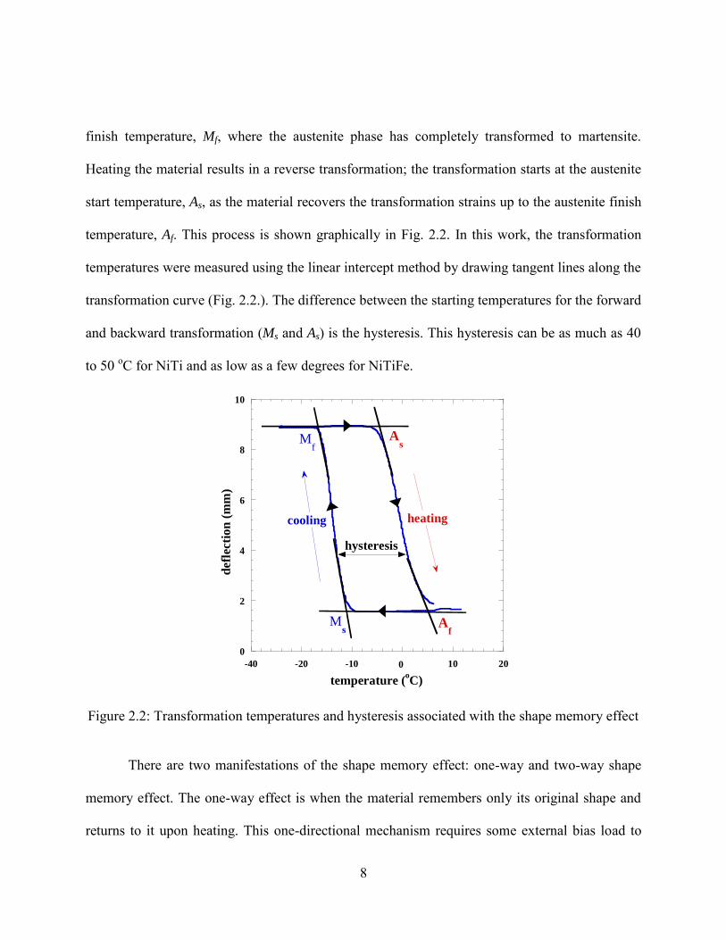
finish temperature, Mf, where the austenite phase has completely transformed to martensite.
Heating the material results in a reverse transformation; the transformation starts at the austenite
start temperature, As, as the material recovers the transformation strains up to the austenite finish
temperature, Af. This process is shown graphically in Fig. 2.2. In this work, the transformation
temperatures were measured using the linear intercept method by drawing tangent lines along the
transformation curve (Fig. 2.2.). The difference between the starting temperatures for the forward
and backward transformation (Ms and As) is the hysteresis. This hysteresis can be as much as 40
to 50 oC for NiTi and as low as a few degrees for NiTiFe.
0
2
4
6
8
10
-40 -20 -10 0 10 20
defl
ecti
on
(m
m)
temperature (oC)
Ms
Mf
As
Af
heatingcooling
hysteresis
Figure 2.2: Transformation temperatures and hysteresis associated with the shape memory effect
There are two manifestations of the shape memory effect: one-way and two-way shape
memory effect. The one-way effect is when the material remembers only its original shape and
returns to it upon heating. This one-directional mechanism requires some external bias load to

9
take the material to the desired deformed shape at low temperatures (e.g., biased actuators). On
the other hand, two way shape memory refers to the material ability to remember its deformed
and original shape in both phases.
2.1.2 Superelasticity
Superelasticity or pseudoelasticity behavior refers to the ability of shape memory alloys
to transform to martensite during loading at temperatures above Af. During loading, the stress-
induced transformation leads to high strain generation as austenite transforms to stress-induced
martensite without plastic deformation. Upon unloading, the strain is completely recovered at
temperatures above the austenite finish temperature due to the reverse transformation. During
this transformation, there is no twinned martensite and macroscopic deformation is primarily
obtained during the phase transformation due to the applied stress (Fig. 2.3).
: Titanium : Nickel
Figure 2.3: Superelasticity: (a) austenite (b) stress-induced martensite (c) shape recovery on reverse transformation to austenite
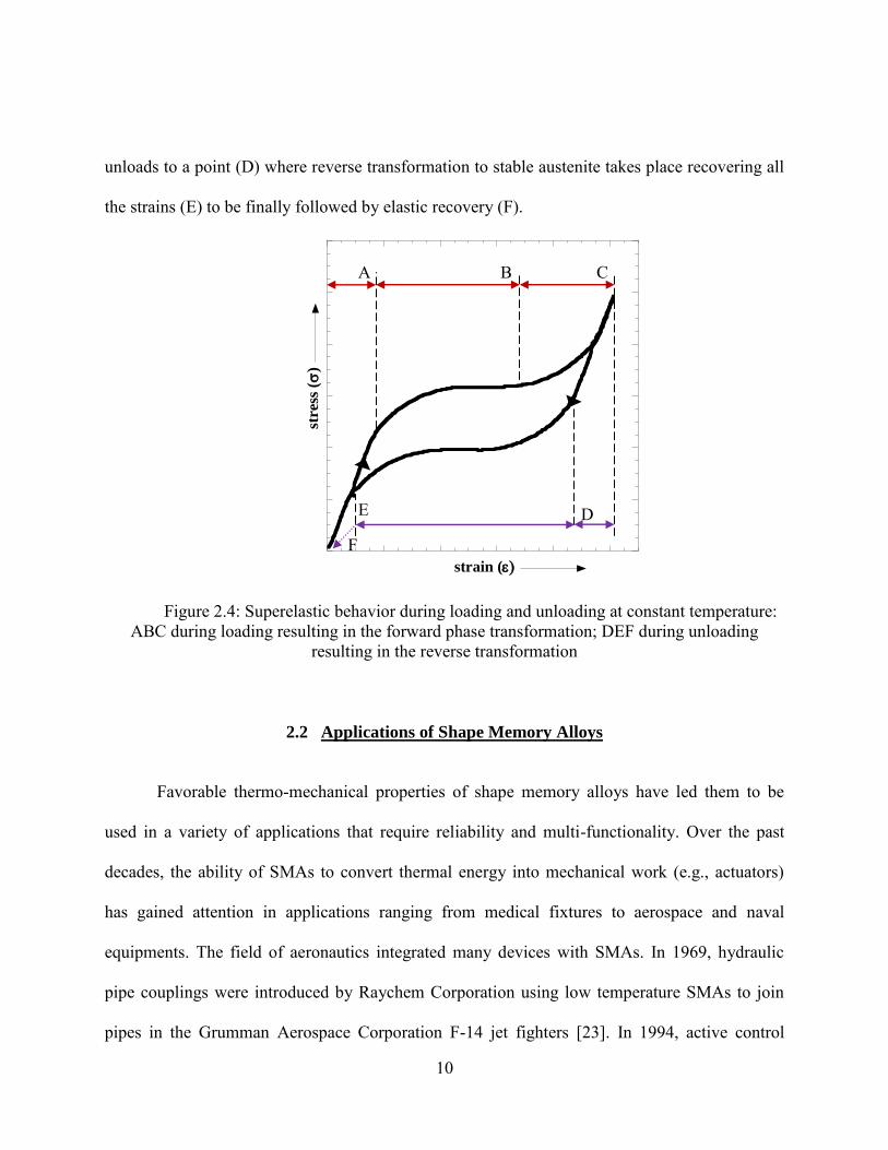
Figure 2.4 shows a typical superelastic loading cycle under isothermal conditions.
Starting from a temperature above Af with no load, a stress is applied that causes elastic
deformation (A) followed by formation of stress-induced martensite (B). Further loading results
in elastic deformation of the detwinned martensite (C). During unloading, martensite elastically
loading
T >Af
unloading
(
a)
(
b)
(
c)
10
unloads to a point (D) where reverse transformation to stable austenite takes place recovering all
the strains (E) to be finally followed by elastic recovery (F).
stre
ss (
)
strain (
Figure 2.4: Superelastic behavior during loading and unloading at constant temperature: ABC during loading resulting in the forward phase transformation; DEF during unloading
resulting in the reverse transformation
2.2 Applications of Shape Memory Alloys
Favorable thermo-mechanical properties of shape memory alloys have led them to be
used in a variety of applications that require reliability and multi-functionality. Over the past
decades, the ability of SMAs to convert thermal energy into mechanical work (e.g., actuators)
has gained attention in applications ranging from medical fixtures to aerospace and naval
equipments. The field of aeronautics integrated many devices with SMAs. In 1969, hydraulic
pipe couplings were introduced by Raychem Corporation using low temperature SMAs to join
pipes in the Grumman Aerospace Corporation F-14 jet fighters [23]. In 1994, active control
A B C
D E
F
11
SMA release bolts developed by the TiNi Alloy Company were used for release mechanisms in
the spacecraft Clementine [24]. Shape memory alloy powered adaptive aircraft inlet internal
walls was employed by NASA Langley Research Center (NASA LaRC) and the Office of Naval
Research (ONR) in The Smart Aircraft and Marine Project System DemonstratiON
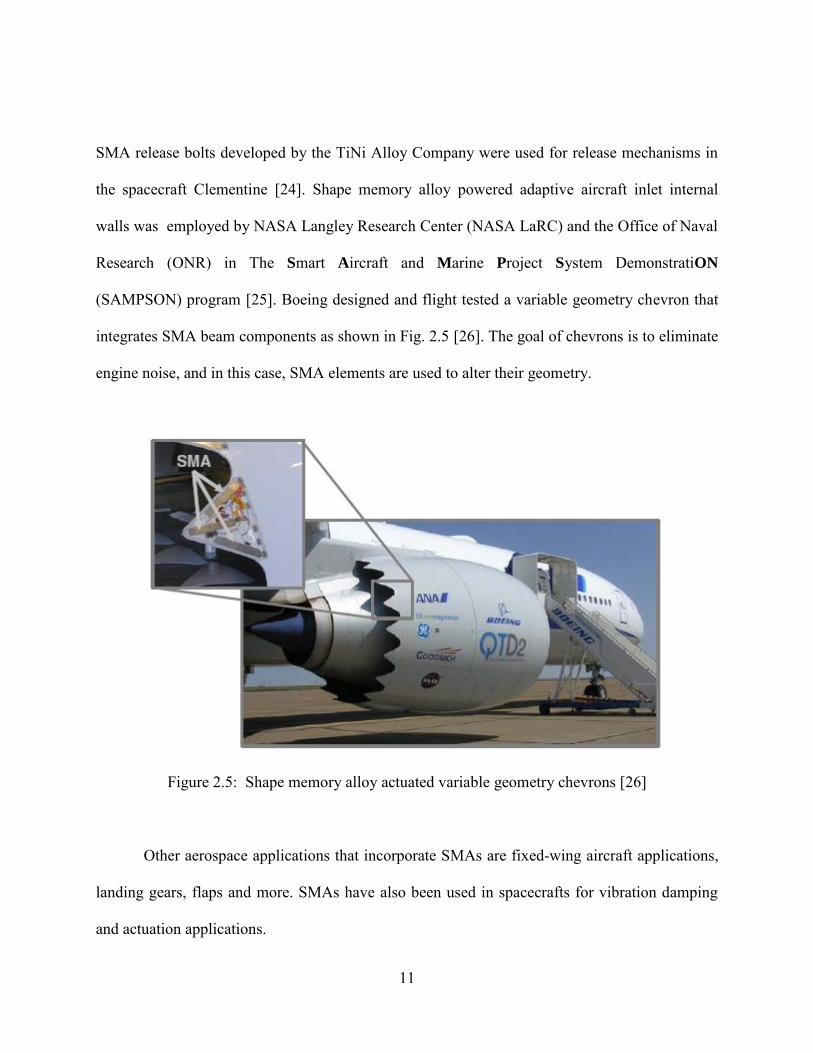
(SAMPSON) program [25]. Boeing designed and flight tested a variable geometry chevron that
integrates SMA beam components as shown in Fig. 2.5 [26]. The goal of chevrons is to eliminate
engine noise, and in this case, SMA elements are used to alter their geometry.
Figure 2.5: Shape memory alloy actuated variable geometry chevrons [26]
Other aerospace applications that incorporate SMAs are fixed-wing aircraft applications,
landing gears, flaps and more. SMAs have also been used in spacecrafts for vibration damping
and actuation applications.

12
Another major field that uses shape memory alloys is the medical industry. Applications
such as orthodontic wires, stents, lengthening limbs and cardiovascular and orthopedic
applications all integrate SMAs in some form to help provide better performance. There are
many other fields besides the ones mentioned here that benefit from advantageous attributes of
SMAs such us transportation industry, civil industry and every day products and more. However,
they are not described in detail since the shape memory effect rather than the superelastic effect
is the focus of this thesis.
2.3 The R-Phase in NiTi System
Among many classes of shape memory alloys, near equi-atomic NiTi alloys are the most
commonly used. These alloys exhibit both the shape memory effect and superelastic behavior as
they transform from the high temperature, cubic (B2) austenite phase to the low temperature,
monoclinic (B19') martensite phase. In most cases, the transformation temperatures of NiTi
occur between room temperature and 100 °C accompanied by a wide hysteresis of about 40 °C.
Applications that require low temperature operation cannot use these alloys; consequently,
modification of binary NiTi is necessary to shift the transformation temperatures and reduce the
hysteresis to fit specific limits. Formation of a stable intermediate R-phase with improved fatigue
response and reduced hysteresis, suppresses the phase transformation and shifts it to lower
temperatures (below 0 °C) [13, 14]. The R-phase can be introduced by annealing below the
recrystallization temperature after cold-working [27, 28], ageing after solution treatment, thermal
cycling or adding a ternary element such as iron [16]. Several studies have shown the multi-stage
R-phase transformation to be transient in binary NiTi and nickel rich systems that do not suit
13
commercial applications [29, 30]. Addition of a ternary alloy such as Fe, on the other hand,
offers phase transformations at low temperature with stable characteristics. The cubic austenite
to trigonal R-phase transformation in NiTiFe is associated with a narrow hysteresis (~ 2 oC) and
better fatigue life due to low strains (~1%) when compared to the B19' phase.
2.4 Thermal Switches
Demand for effective thermal control devices for space and ground-base applications has
grown due to advanced technological thermal management needs. In the aerospace industry,
thermal control is accomplished via single-phase cooling systems or two-phase technologies
such as capillary pumped loops (CPLs) or loop heat pipes (LHPs), among others. In most cases,
it is desirable to thermally isolate the system to create an adiabatic environment but most thermal
control devices do not provide such flexibility. The use of thermal switches to couple/decouple
heat sinks from the heat source has proven to be advantageous. Most of the thermal switches
have the objective of affecting heat flow to reduce or eliminate parasitic heat loads, isolate
vibrations and provide high heat flux during engagement. A wide range of thermal switches have
been developed for application at temperatures ranging from 673 oC to -272 oC [1-4]. Mechanical
thermal switches such as differential thermal expansion switches (Fig. 2.6) are based on the
differences in the coefficient of thermal expansion (CTE) of two materials. During cooling, the
outer element comprising of the high CTE material contracts around a low CTE material causing
the switch to make contact [31]. As the temperature is elevated, the high CTE material expands
more than the low CTE material causing thermal isolation. Heat transfer through the switch is
14
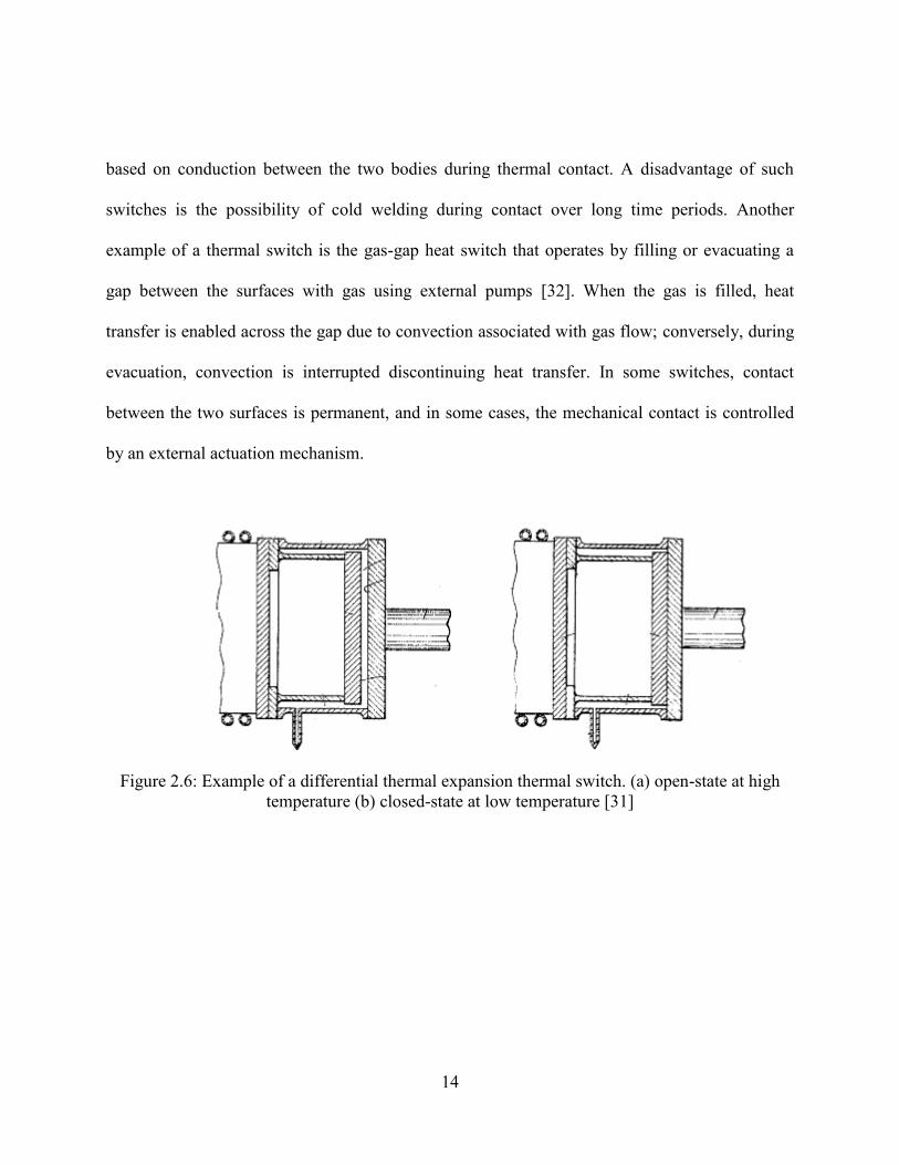
based on conduction between the two bodies during thermal contact. A disadvantage of such
switches is the possibility of cold welding during contact over long time periods. Another
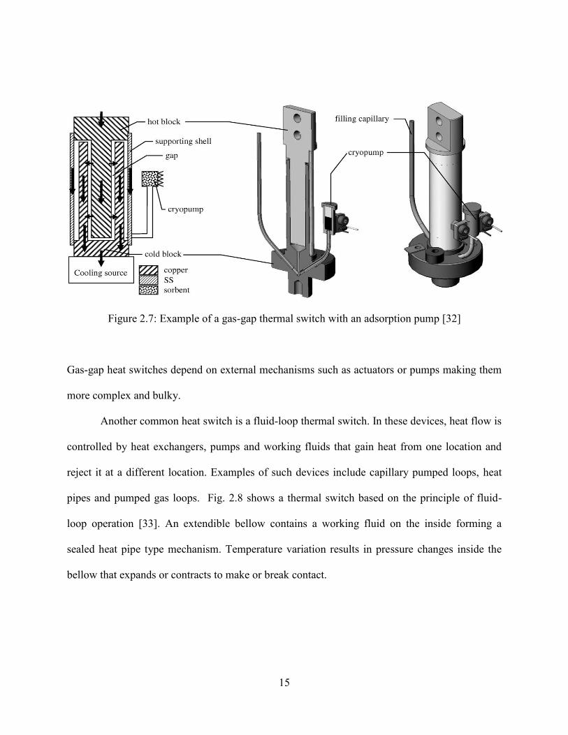
example of a thermal switch is the gas-gap heat switch that operates by filling or evacuating a
gap between the surfaces with gas using external pumps [32]. When the gas is filled, heat
transfer is enabled across the gap due to convection associated with gas flow; conversely, during
evacuation, convection is interrupted discontinuing heat transfer. In some switches, contact
between the two surfaces is permanent, and in some cases, the mechanical contact is controlled
by an external actuation mechanism.
Figure 2.6: Example of a differential thermal expansion thermal switch. (a) open-state at high temperature (b) closed-state at low temperature [31]
(
a)
(
b)
15
Figure 2.7: Example of a gas-gap thermal switch with an adsorption pump [32]
Gas-gap heat switches depend on external mechanisms such as actuators or pumps making them
more complex and bulky.
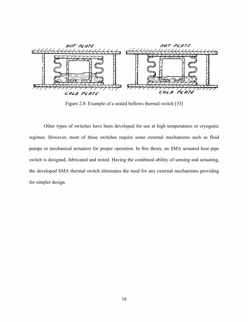
Another common heat switch is a fluid-loop thermal switch. In these devices, heat flow is
controlled by heat exchangers, pumps and working fluids that gain heat from one location and
reject it at a different location. Examples of such devices include capillary pumped loops, heat
pipes and pumped gas loops. Fig. 2.8 shows a thermal switch based on the principle of fluid-
loop operation [33]. An extendible bellow contains a working fluid on the inside forming a
sealed heat pipe type mechanism. Temperature variation results in pressure changes inside the
bellow that expands or contracts to make or break contact.
16
Figure 2.8: Example of a sealed bellows thermal switch [33]
Other types of switches have been developed for use at high temperatures or cryogenic
regimes. However, most of these switches require some external mechanisms such as fluid
pumps or mechanical actuators for proper operation. In this thesis, an SMA actuated heat pipe
switch is designed, fabricated and tested. Having the combined ability of sensing and actuating,
the developed SMA thermal switch eliminates the need for any external mechanisms providing
for simpler design.

17
CHAPTER THREE: NiTiFe SHAPE MEMORY ALLOY HELICAL
ACTUATORS
Shape memory alloy (SMA) actuators have received renewed interest in the last two
decades due to their unique thermo-mechanical characteristics. These „smart‟ actuators combine
both sensory and actuation capability in a single mechanism due to a temperature induced solid-
state phase transformation that can bring about shape changes against external loads. Reduced
helical spring design equations have been applied to design shape memory alloy compression
and tension helical actuators [34, 35]. This approach yields erroneous approximations due to the
small helix angle assumption and associated neglect of the bending and direct shear effects on
the helix. This chapter reports on the effect of the helix angle on SMA helical springs by direct
comparison between the reduced equations, equations in full form, a finite element model
(FEM), and experimental results. The effects of the spring‟s geometry including the coil radius,
helix angles and extension under load are examined. Due to significant changes in the shear
modulus during the martensitic phase transformation (~300%), the response of both the high
temperature cubic, B2, austenitic phase as well as the low temperature trigonal R-phase are
quantified. Axial extensions and the accompanying stress distributions along the coil are also
presented.
3.1 Helical Spring Analyses
Helical tension/compression springs have been widely used in a variety of applications
due to their elastic ability to extend or contract and recover upon application or removal of

18
functional loads. Helical springs are used as mechanical devices that store elastic potential
energy and generate stroke as a function of applied load. However, advanced thermo-mechanical
technologies require helical springs to work as actuators with the ability to sense and actuate in
response to other parameters in addition to load. Shape memory alloy helical springs are
advantageous over conventional spring materials in their thermo-elastic response. They couple
thermal and mechanical effects and produce adequate actuation energy densities. Shape memory
alloy helical springs generate stroke as a function of applied stress and/or temperature making
them suitable for sensing and actuating applications where changes in temperature are a factor.
It is as important to decide on the correct theoretical approach with minimum
assumptions to design a helical actuator. A frequently adopted approach for SMA helical spring
design has been the application of the reduced form of torsion and bending theories. These
simplified formulations are insufficient to capture the bending and helix effects resulting in
deviations between experimental and theoretical predictions. Several approaches have been
adopted to solve the static response of helical springs, e.g., the transfer matrix method (TMM)
[36], the boundary element method (BEM) [37-39], or the finite element method (FEM) [40-42].
However, the implementation of the analyses has mostly ignored the effect of the helical angle
for simplification. In this work, effects of the helix angle in SMA helical springs were
investigated by direct comparison between the reduced equations, equations in full form, a finite
element model (FEM) and experimental results. Geometrical and displacement constraints are
described with the aid of a free body diagram. The displacement and stress distributions along
the coil are quantified for both the austenite and the R-phase.

19
3.2 Helical Shape Memory Alloy Actuators
Shape memory alloys have great potential in actuator applications due to their high
strength-to-weight ratio and work output associated with the phase transformation. Conventional
systems such as hydraulic or pneumatic actuators transmit high power in large scale actuators,
but their performance is significantly reduced as they scale down in size. This limitation is
addressed by using SMA actuators in the form of helical springs. Helical actuators provide larger
stroke when compared to other forms such as wire, beams or strips (e.g., Ref. [18]). Other
thermal actuators have been used in the past such as wax or bimetal actuators, but these methods
are affected by several limitations such as slow response time or geometrical constraints [43].
The use of SMA helical actuators eliminates these limitations and provides greater advantages
over other alternatives. Motion in SMA actuators is generated by conversion of thermal energy
(heat addition or removal) to mechanical energy (stroke) due to the temperature-induced solid-
state phase transformation described in the preceding sections.
Throughout this study, the initial undeformed length, Lo, of the spring exists in the high
temperature austenite phase. In this phase, the spring constant is at its maximum value due to the
high shear modulus, (e.g., 20 GPa). Applying a pre-load, P, introduces an initial extension, initial,
which takes the spring to a new pre-deformed length. As the material undergoes a temperature
induced phase transformation to the R-phase, the spring stiffness reduces due to reduction in the
shear modulus, (e.g., 8 GPa), and exhibits a final deflection, working, to a maximum length, Lm, as
shown in Fig. 3.1.

20
Figure 3.1: SMA helical spring length: (a) high temperature phase (b) low temperature phase
3.3 Helical Shape Memory Alloy Actuator Design
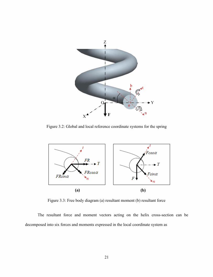
A circular cross-section helical spring subjected to uniaxial loading was examined in this
study as shown in Fig. 3.2 with the adopted global and local orthogonal coordinate systems (O,
X, Y, Z) and (o, t, n, b), respectively. The cross-section of the spring with wire diameter, d, mean
coil diameter, D, and helix angle, subject to a compressive or tensile load, F, experiences
shear force, Fs, and a moment couple, FD/2, that contributes to bending effects as the coil
curvature changes and to twisting effects from the resulting torque (Fig. 3.3a-b) [44]. The single
headed arrow represents the uniaxial force in the indicated direction and the double headed arrow
represents moment about the indicated direction.
no load pre-load max working load
(
b)
heating unloading
cooling loading
initial working
(a) (b)
Lo
21
Figure 3.2: Global and local reference coordinate systems for the spring
Figure 3.3: Free body diagram (a) resultant moment (b) resultant force
The resultant force and moment vectors acting on the helix cross-section can be
decomposed into six forces and moments expressed in the local coordinate system as
(a) (b)
o
X
Z
O
t
n
b
Y
F
22
sin cos2
cos sin2
t
n b t n b n
btb t
S S
DF F
eD
R N F F M M M R F F e
edA y dA
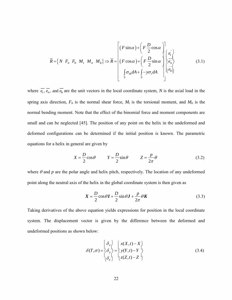
(3.1)
where , , and t n be e e are the unit vectors in the local coordinate system, N is the axial load in the
spring axis direction, Fb is the normal shear force, Mt is the torsional moment, and Mb is the
normal bending moment. Note that the effect of the binomial force and moment components are
small and can be neglected [45]. The position of any point on the helix in the undeformed and
deformed configurations can be determined if the initial position is known. The parametric
equations for a helix in general are given by
cos
2
DX sin
2
DY
2
pZ
(3.2)
where and p are the polar angle and helix pitch, respectively. The location of any undeformed
point along the neutral axis of the helix in the global coordinate system is then given as
cos sin
2 2 2
D D p
X I J K (3.3)
Taking derivatives of the above equation yields expressions for position in the local coordinate
system. The displacement vector is given by the difference between the deformed and
undeformed positions as shown below:
( , )
( , ) ( , )
( , )
x
y
z
x X t X
T y Y t Y
z Z t Z
(3.4)

23
3.3.1 Equations in Reduced Form
The commonly used SMA spring design methodology for actuator applications is based
on a reduced form of general elastic theory. This approach neglects curvature and direct shear
effects by assuming the spring elements as a straight wire in pure torsion. From the simple theory
of torsion [46], every section subjected to a torque experiences a state of pure shear. The
uncorrected stress neglecting direct shear loading and wire curvature may be obtained from
aT G
J R L
(3.5a)
where Ta is the applied torque, J is the polar second moment of area of coil cross-section, G is
the shear modulus, R is the outside radius, and is the angle of twist on a length L. Solving for
the shear stress from Eq. 3.5a yields
3
8FD
d
(3.5b)
where F is the applied load, D is the mean diameter, and d is the wire diameter. However, Eq.
3.5b gives an average stress on the outside edge of the coil. In order to determine the maximum
stresses which occur on the inside of the spring, the latter equation is modified using a correction
factor of the form
max 3
8FD
d
,
1 pure torsion
0.51 shear stress correction factor
4 1 0.615Wahl's factor (Ref. [45])
4 4
s
w
C
C
C C
(3.5c)
24
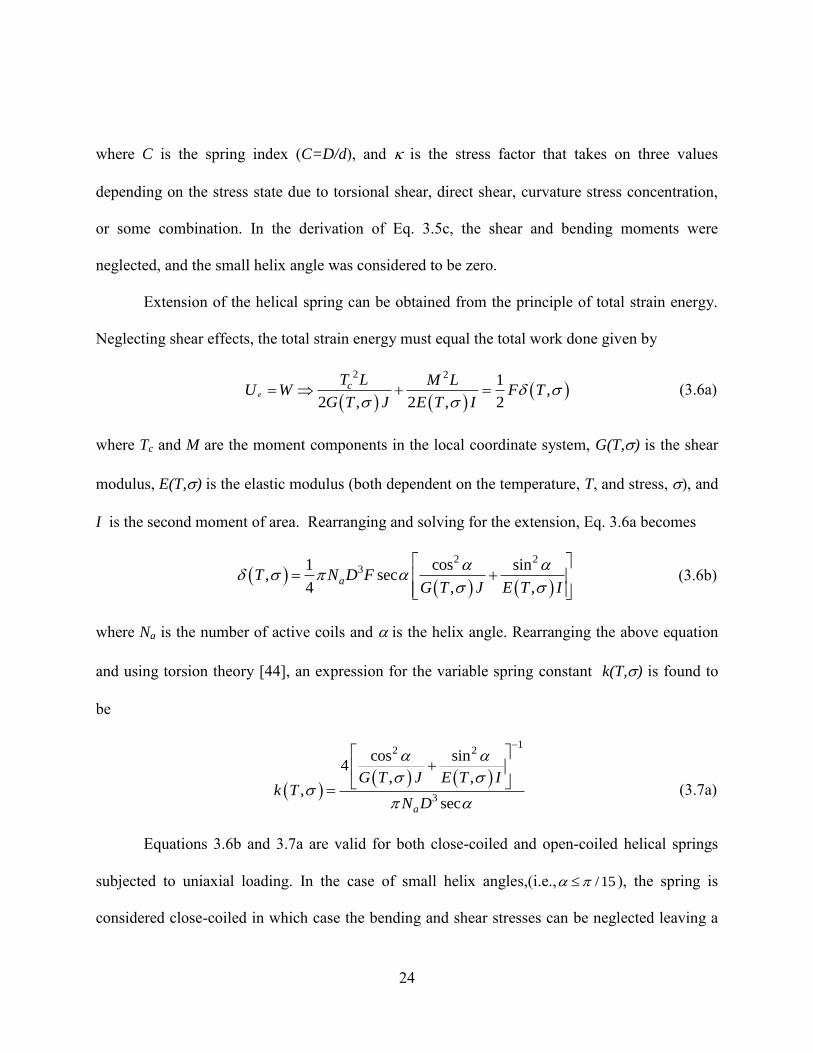
where C is the spring index (C=D/d), and is the stress factor that takes on three values
depending on the stress state due to torsional shear, direct shear, curvature stress concentration,
or some combination. In the derivation of Eq. 3.5c, the shear and bending moments were
neglected, and the small helix angle was considered to be zero.
Extension of the helical spring can be obtained from the principle of total strain energy.
Neglecting shear effects, the total strain energy must equal the total work done given by
2 2 1
,2 , 2 , 2
ecT L M L
U W F TG T J E T I
(3.6a)
where Tc and M are the moment components in the local coordinate system, G(T,) is the shear
modulus, E(T,) is the elastic modulus (both dependent on the temperature, T, and stress, ), and
I is the second moment of area. Rearranging and solving for the extension, Eq. 3.6a becomes
2 231 cos sin
, sec4 , ,
aT N D FG T J E T I
(3.6b)
where Na is the number of active coils and is the helix angle. Rearranging the above equation
and using torsion theory [44], an expression for the variable spring constant k(T,) is found to
be
12 2
3
cos sin4
, ,,
seca
G T J E T Ik T
N D
(3.7a)
Equations 3.6b and 3.7a are valid for both close-coiled and open-coiled helical springs
subjected to uniaxial loading. In the case of small helix angles,(i.e., /15 ), the spring is
considered close-coiled in which case the bending and shear stresses can be neglected leaving a

25
predominantly torsional stress state. Assuming small helix angles (i.e., cos = 1 and sin = 0),
Eqs. 3.6b and 3.7a reduce to conventional equations for close-coiled helical springs.
For small ,
2 20 cos 1 sin 0and
31 1 1 0,
4 1 , ,aT N D F
G T J E T I
3
4
1 1,
4,
32
aT N D Fd
G T
3
4
8,
,
aN D FT
G T d
(3.7b)
Similarly,
4
3
,,
8 a
G T dk T
N D
(3.7c)
The shear modulus can be quantified using shape memory alloy models that take into
account the degree of martensitic transformation [47].
For helical SMA springs, these equations are applied to the high and low temperature
phases as the shear modulus changes with temperature or stress. As mentioned previously, this
approach neglects the effect of direct shear and bending stress as the load is applied. In the
following section, the full theory is examined and compared with the discussion in this section.
26
3.3.2 Equations in Full Form
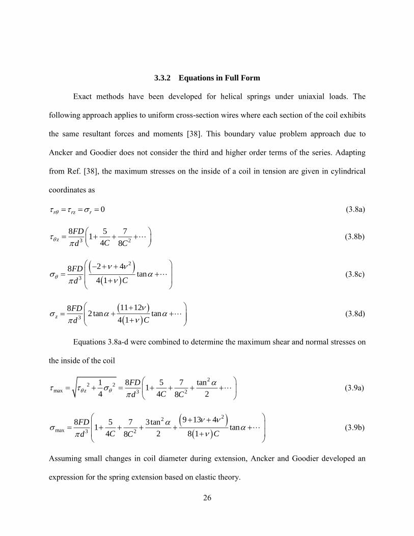
Exact methods have been developed for helical springs under uniaxial loads. The
following approach applies to uniform cross-section wires where each section of the coil exhibits
the same resultant forces and moments [38]. This boundary value problem approach due to
Ancker and Goodier does not consider the third and higher order terms of the series. Adapting
from Ref. [38], the maximum stresses on the inside of a coil in tension are given in cylindrical
coordinates as
0r rz r (3.8a)
3 2
8 5 71
4 8z
FD
Cd C
(3.8b)
2
3
2 48tan
4 1
FD
Cd
(3.8c)
3
11 1282 tan tan
4 1z
FD
Cd
(3.8d)
Equations 3.8a-d were combined to determine the maximum shear and normal stresses on
the inside of the coil
22 2
max 3 2
1 8 5 7 tan1
4 4 28z
FD
Cd C
(3.9a)
22
max 3 2
9 13 48 5 7 3tan1 tan
4 2 8 18
FD
C Cd C
(3.9b)
Assuming small changes in coil diameter during extension, Ancker and Goodier developed an
expression for the spring extension based on elastic theory.

27
32
4 2
38 31 tan
2 116
aPD N
Gd C
(3.10)
These equations yield small errors when small helix angles are used. In the case of large
extensions, modified equations are used and can be found in Ref. [45].
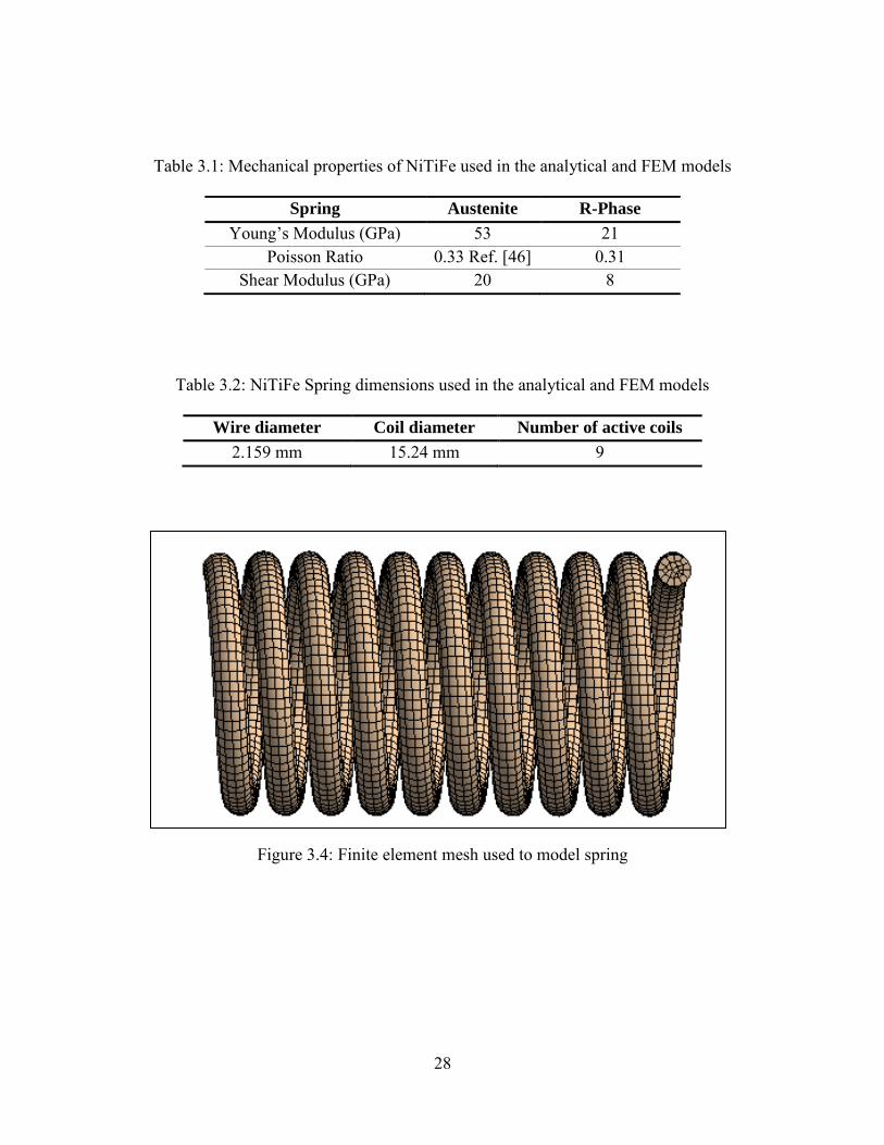
3.3.3 Finite Element Method
The finite element method (FEM) was used to compare the two approaches used for helical
spring design. Since the resultant moments, forces and the stress distributions are equal at any
given section, only half turn of the helical spring are shown. The model was discretized using
4312 solid elements (Brick 20 node 186) using ANSYS® and ANSYS Workbench®. Figure 3.4
shows the finite element mesh used. Boundary conditions were applied to obtain the stress as the
spring extends. Elastic deformation was solely considered. One end of the coil was fully
constrained against translation and rotation to simulate the operating conditions of the SMA
actuators used in the thermal switch. An axial load along the spring axis was applied along the
other end. The material properties and dimensional parameters used in the study are listed in
Tables 3.1 and 3.2 respectively. The macroscopic shear and Young‟s moduli for both phases
were determined from experimental data obtained from this work assuming linear isotropic
behavior. However, it is important to note that NiTiFe alloy exhibits anisotropic behavior and
nonlinearity due to detwinning during the martensitic phase transformation that was not
considered here. Also, these mechanical properties were taken to be constant in each phase and
not vary with stress or temperature. Poisson‟s ratios used are those of a NiTi alloy [48].
28
Table 3.1: Mechanical properties of NiTiFe used in the analytical and FEM models
Spring Austenite R-Phase
Young‟s Modulus (GPa) 53 21 Poisson Ratio 0.33 Ref. [46] 0.31
Shear Modulus (GPa) 20 8
Table 3.2: NiTiFe Spring dimensions used in the analytical and FEM models
Wire diameter Coil diameter Number of active coils
2.159 mm 15.24 mm 9
Figure 3.4: Finite element mesh used to model spring
29
3.3.4 Comparisons between Elastic Theory and the Finite Element Method
The maximum shear stresses, z, for a small helix angle, ≈ 2°, were calculated using
Eqs. 3.5b, 3.5c, 3.8b, and compared with results from a finite element model. This analysis
showed that the shear stresses are maximum at the inner radius of the coil, which is not captured
by Eq. 3.5b which assumes pure torsion. Equation 3.5c derived by Wahl provides both the
torsional shear and bending shear on the neutral axis of a cantilever beam with circular cross-
section. Equation 3.8b takes into account the maximum shear stresses that occur at the inner
radius of the spring. Figure 3.6 shows the z shear stress distribution in a cross-section of a
spring coil from FEM. The boundary conditions and constraints were imposed to simulate a
uniaxial spring in tension for different applied loads with its ends fixed against rotation. It is
shown that the maximum shear occurs at the inner radius of the spring for all loads considered.
This was also verified using different helix angles of = 5, 10, 15 and 20 degrees.
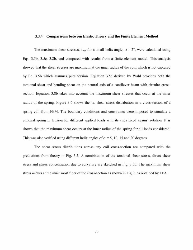
The shear stress distributions across any coil cross-section are compared with the
predictions from theory in Fig. 3.5. A combination of the torsional shear stress, direct shear
stress and stress concentration due to curvature are sketched in Fig. 3.5b. The maximum shear
stress occurs at the inner most fiber of the cross-section as shown in Fig. 3.5a obtained by FEA.
30
Figure 3.5: Shear stress distribution across coil section in a helical SMA spring: (a) FEA (b) prediction from theory (spring axis to the right)
Figure 3.6 presents the shear stress distribution, z, on the wire‟s cross-section for a
helical spring in tension. Comparisons of the theoretical z shear stress values with the finite
element analysis (FEA) are shown in Fig. 3.7. FEA results are within 1% and 2% error from the
values obtained using Equations 3.5c and 3.8b respectively. However Equation 3.5b, which
assumes pure torsion in the coil, differs by 18 % from the FEA results.
(a) (b)
z (MPa)

31
Figure 3.6: z shear stress distribution for a spring cross-section with small helix angle ≈ 2° (austenite, spring axis to the right)
F = 1 N F = 5 N
F = 9 N F = 20 N
z (MPa) z (MPa)
z (MPa) z (MPa)

32
0
20
40
60
80
100
0 2 4 6 8 10
Reduced form (Eq. 3.5b)
Wahl (Eq. 3.5c)
Ancker & Goodier (Eq. 3.8b)
FEA
shear s
tres
s (M
Pa)
extension (mm)
Figure 3.7: Comparison of maximum shear stress (z) using elastic theory and FEA (austenite)
To show that the helix angle has an effect on the stress distribution along the coil, the
normal stresses along the spring axis, z, were investigated using FEA and Eq. 3.8d. Figure 3.8
shows the normal stress distribution for different helix angles in the austenite phase using a load
of F = 9 N. Similar to the shear stress (z), the maximum normal stresses occur at the inner
radius of the coil. Figure 3.9 shows the results obtained using both Eq. 3.8d and FEA for various
helix angles.

33
Figure 3.8: z distribution for F= 9 N in helical coil (austenite)
= 2° = 10°
= 20°
z (MPa) z (MPa)
z (MPa) z (MPa)
= 15°
34
0
10
20
30
40
50
60
70
0 5 10 15 20 25
Ancker & Goodier (Eq. 3.8d)
FEA
no
rma
l st
res
s
z (M
Pa
)
helical angle (deg.)
F = 20 N
F = 9 N
F = 5 N
F = 1 N
Figure 3.9: z as a function of helical angle for various loads (austenite)
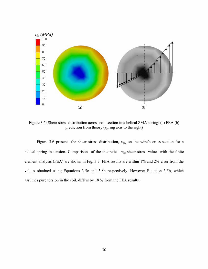
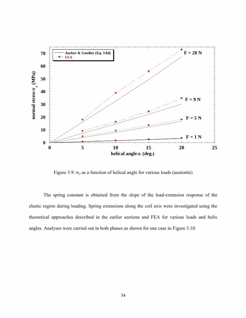
The spring constant is obtained from the slope of the load-extension response of the
elastic region during loading. Spring extensions along the coil axis were investigated using the
theoretical approaches described in the earlier sections and FEA for various loads and helix
angles. Analyses were carried out in both phases as shown for one case in Figure 3.10.
35
Figure 3.10: Spring displacement in tension for small helix angle ≈ 2° (austenite, bottom of spring fixed and load applied at the top end)
F = 1 N F = 5 N
F = 9 N F = 20 N
(mm) (mm)
(mm) (mm)

36
Spring extensions as a function of the helical angle are shown for the austenite phase in
Fig. 3.11 and for the R-phase in Fig. 3.12. For small helix angles and small loads, the equations
give similar results for both phases. However, upon increasing the helical angle and the load, the
results diverge due to large extension. Therefore, for springs that are not close-coiled, the
simplified approaches do not capture the true deformation of the spring and the complete theory
has to be used for accurate results.
0
1
2
3
4
5
6
0 5 10 15 20 25
Reduced form (Eq. 3.7b)
Modified form (Eq. 3.6b)
Ancker & Goodier (Eq. 3.10)
FEA
exte
nsi
on
(m
m)
helical angle (deg.)
F = 1 N
F = 5 N
F = 9 N
Figure 3.11: Correlation between spring extension and helical angle (austenite)

37
0
2
4
6
8
10
12
14
16
0 5 10 15 20 25
Reduced form (Eq. 3.7b)
Modified form (Eq. 3.6b)
Ancker & Goodier (Eq. 3.10)
FEA
exte
nsi
on
(m
m)
helical angle (deg.)
F = 1 N
F = 5 N
F = 9 N
Figure 3.12: Correlation between spring extension and helical angle (R-phase)
The comparisons between FEM and theory (both in reduced and full forms) presented in
this section highlight the limitations of the theory. It was shown from FEA that maximum
stresses occurred at the inner radius of the springs which in turn were predicted by the equations
from elastic theory in full form and not by the ones in reduced or simplified form. Furthermore,
it was established that the spring extension is influenced by the helical angle and which should
be considered especially in the design of open-coiled springs.
38
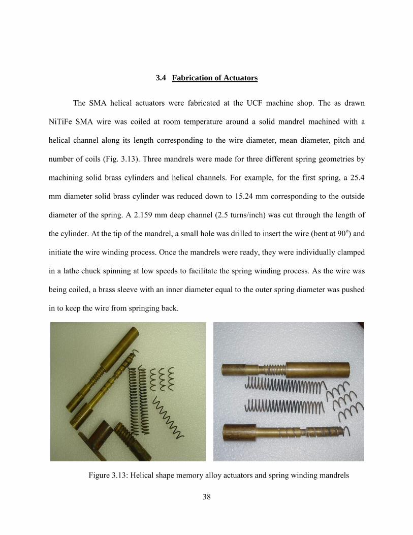
3.4 Fabrication of Actuators
The SMA helical actuators were fabricated at the UCF machine shop. The as drawn
NiTiFe SMA wire was coiled at room temperature around a solid mandrel machined with a
helical channel along its length corresponding to the wire diameter, mean diameter, pitch and
number of coils (Fig. 3.13). Three mandrels were made for three different spring geometries by
machining solid brass cylinders and helical channels. For example, for the first spring, a 25.4
mm diameter solid brass cylinder was reduced down to 15.24 mm corresponding to the outside
diameter of the spring. A 2.159 mm deep channel (2.5 turns/inch) was cut through the length of
the cylinder. At the tip of the mandrel, a small hole was drilled to insert the wire (bent at 90o) and
initiate the wire winding process. Once the mandrels were ready, they were individually clamped
in a lathe chuck spinning at low speeds to facilitate the spring winding process. As the wire was
being coiled, a brass sleeve with an inner diameter equal to the outer spring diameter was pushed
in to keep the wire from springing back.
Figure 3.13: Helical shape memory alloy actuators and spring winding mandrels
39
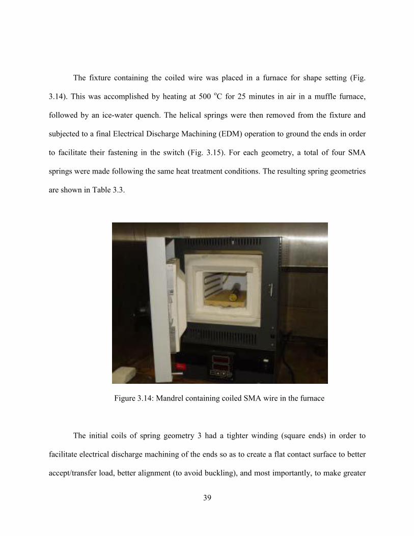
The fixture containing the coiled wire was placed in a furnace for shape setting (Fig.
3.14). This was accomplished by heating at 500 oC for 25 minutes in air in a muffle furnace,
followed by an ice-water quench. The helical springs were then removed from the fixture and
subjected to a final Electrical Discharge Machining (EDM) operation to ground the ends in order
to facilitate their fastening in the switch (Fig. 3.15). For each geometry, a total of four SMA
springs were made following the same heat treatment conditions. The resulting spring geometries
are shown in Table 3.3.
Figure 3.14: Mandrel containing coiled SMA wire in the furnace
The initial coils of spring geometry 3 had a tighter winding (square ends) in order to
facilitate electrical discharge machining of the ends so as to create a flat contact surface to better
accept/transfer load, better alignment (to avoid buckling), and most importantly, to make greater

40
surface contact (approx. ~ 290o) for improved heat conduction during operation. Given this
modification, spring geometry 3 was used in the subsequent work reported here even though
some initial results from the other geometries are presented for completeness.
Figure 3.15: Spring geometry 3 after shape setting and final electrical discharge machining to increase contact
Table 3.3: Shape memory alloy spring geometries (wire diameter 2.159 mm)
Spring D (mm) Pitch (mm) Free length (mm) End condition
1 17.8 10.9 63.5 Plain 2 12.7 15.9 50.8 Ground 3 13.1 12.7 63.5 Cut
Table 3.4: Shape memory alloy spring constants (wire diameter 2.159 mm)
Spring constant N/mm
Spring Austenite R-Phase
1 1.878 0.482 2 8.587 2.209 3 4.283 1.517

41
Prior to installing the springs in the thermal switch, mechanical testing was conducted on
a servo-hydraulic load frame to determine the spring constants in the austenitic state at room
temperature. The SMA springs were placed on flat grips in order to apply a gradual load in
compression. Load-displacement data was collected for each spring using a 220 N load cell and a
LVDT attached to the load frame upper grip. Results corresponding to the four springs with
spring geometry 3 are plotted in Fig. 3.16.
0
5
10
15
20
25
30
35
0 1 2 3 4 5 6 7
spring #1spring #2spring #3spring #4
load
(N
)
extension (mm)
Figure 3.16: Load-extension response of the SMA springs at room temperature
The slopes of the load-extension lines represent the spring constants under loads not
exceeding the elastic limit of the alloys and are reported in Table 3.4. The average spring
constant of the four springs with spring geometry 3 was 4.283 N/mm and this corresponds to a
shear modulus of 19.4 GPa for austenite from Equation 3.7a compared to the initial value of 21
GPa.
42
Sets of stainless steel bias springs (four each) were designed and custom made to provide
the necessary force to extend the switch during the SMA phase transformation. The calculations
are presented in Appendix A. The geometry of the bias springs was selected with an inside
diameter large enough to fit over the SMA springs and avoid contact during extension. They
were made longer than the SMA springs in order to provide a bias force during the open and
closed positions of the switch. The bias spring constants were selected to be between that of the
austenite and R-phase SMA spring constants to provide force balance during actuation. Multiple
bias springs (sets of four), were obtained in order to modify the switch extension as needed.
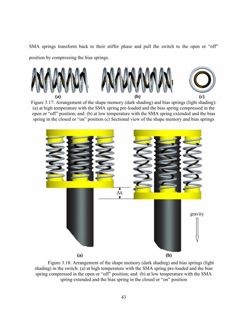
3.5 Thermal Switch Actuation
Actuation of the thermal switch occurs through a combination of the SMA springs and
the compression stainless steel bias springs connected in parallel between the switch base and a
moving plate (Fig. 3.17-18). The actuation is characterized as a push-pull mechanism activated
by a change in temperature. The SMA actuators were designed to hold (pull) the switch in the
open or “off” position in the high temperature phase (e.g., day cycle on the lunar surface).
Initially at room temperature, the bias springs are compressed by the SMA spring force to keep
the switch open. In this state, the force of the SMA springs in the austenite phase is greater than
the total bias force (with contributions from the weight of the components, internal heat pipe
pressure and the unextended bias springs). As the temperature drops below the transformation
temperature, the SMA springs transform to their more compliant phase as the compressed bias
springs overcome the SMA stiffness and extend. At this instance, the total bias force pushes the
moving plate causing the switch to close. Conversely, during the reverse transformation, the
43
SMA springs transform back to their stiffer phase and pull the switch to the open or “off”
position by compressing the bias springs.
Figure 3.17: Arrangement of the shape memory (dark shading) and bias springs (light shading): (a) at high temperature with the SMA spring pre-loaded and the bias spring compressed in the open or “off” position; and (b) at low temperature with the SMA spring extended and the bias
spring in the closed or “on” position (c) Sectional view of the shape memory and bias springs
Figure 3.18: Arrangement of the shape memory (dark shading) and bias springs (light shading) in the switch: (a) at high temperature with the SMA spring pre-loaded and the bias spring compressed in the open or “off” position; and (b) at low temperature with the SMA
spring extended and the bias spring in the closed or “on” position
(a) (b)
(a) (b) (c)
gravity

44
CHAPTER FOUR: VARIABLE LENGTH TWO-PHASE HEAT PIPE
4.1 Overview
A heat pipe incorporates heat transfer mechanisms that provide considerable advantages
over other heat transfer devices due to larger heat transport even with very small temperature
gradients. Heat pipes based on two-phase systems offer greater thermal capacity during working
fluid phase changes with smaller mass flow rates [49]. The first engineering application was
investigated and designed in the early nineteen century by A.M. Perkins. This early age
thermosyphon was used in a steam boiler to transfer heat from a furnace [50, 51]. The name
“heat pipe” was first introduced by Grover in the 1960s when he was studying phase changes in
a heat transport device [52]. Since then, heat pipes have been employed in various applications in
the aerospace, electric power, chemical and HVAC industries. Design terminology and operating
conditions of closed form heat pipes (thermosyphons) have been outlined by many researchers
and various theories have been developed for the mechanism of heat and mass transfer involving
two-phase flow [53-58]. For example, Wang et al. [59] used computational fluid dynamics
(CFD) to study two-phase flow and phase changes involving porous media. Tabatabi and Faghri
investigated the two-phase flow characteristics and transition boundaries in micro tubes [60].
Wang and Vafai evaluated the transient thermal performance of heat pipes [61].
Heat pipes can be considered to be composed of three main sections: an evaporator (heat
source) section, an adiabatic section and a condenser (heat sink) section (Fig. 4.1). As the
working fluid liquid pool at the evaporator end heats up, bubbles form and move upward as they
grow in size and get rejected from the liquid pool by buoyancy forces. The working fluid

45
transforms to vapor due to heat addition, and absorbs an amount of heat equivalent to the latent
heat of vaporization. As the vapor moves upward toward the condenser at lower temperature, the
working fluid vapor condenses and flows back to the evaporator region in the form of a film or
droplets assisted by gravity in the case of a thermosyphon. Finally, the liquid reaches the bottom
of the heat pipe, mixes with the liquid pool and evaporates again allowing a heat gain/release
mechanism inside the heat pipe. The heat pipe used in this work is a gravity-assisted heat pipe
where the condensate streams downward assisted by gravitational forces and no capillary system
is used. Due to this gravity-driven requirement, the condenser region has to be above the
evaporator region for proper operation.
Figure 4.1: Sections in a heat pipe involving two-phase flow
direction of
gravity
vapor
Qc
Qe
evaporator (Te, Pe)
condenser (Tc, Pc)
adiabatic region
Qout
Qloss to surroundings
liquid pool
vapor flow
condensate flow
bubble formation
Qstored
Qin
n
heat output (e.g., to space environment)
heat input (from heat source)
vapor
Qc
Qe
46
In general, the energy balance for a defined control volume can be expressed as
in stored generated outE E E E (4.1)
Assuming the heat leaving the evaporator with uniform heat addition is equal to the heat entering
the condenser with uniform temperature distribution, energy balance in a heat pipe gives
in stored loss outQ Q Q Q (4.2)
The heat discharged, Qe, and heat received, Qc, can be expressed as
, ,( )e e e s e e satQ h A T T (4.3a) , ,( )c c c c sat s cQ h A T T (4.3b)
where h is the heat transfer coefficient, A is the internal surface area, T is the wall temperature,
Tsat is the saturation temperature, and ‘e’, ‘c’ and ‘s’ stand for the evaporator, condenser and
surface respectively. The surface temperature of both regions is taken as the average temperature
of the entire region.
Given the constraints associated with the operation of the switch in this work, the heat
pipe has to be entirely sealed and at the same time allow movements enforced by the SMA
actuators. The heat pipe used here accomplishes heat transfer through boiling, evaporation and
condensation of the selected working fluid. The analyses presented are based on theoretical
models of pool boiling and parametric effects, evaporation, and laminar film condensation on a
vertical wall [62-64]. Various parameters such as operating temperature and pressure, working
47
fluid volume, end boundary conditions, and transport limitations are considered to ensure
maximum performance.
4.2 Closed Two-Phase Thermosyphon Design
The underlying theory of a closed two-phase thermosyphon (CTPT) is based on bubble
formation and liquid evaporation as the lower end of the pipe is heated. The vapor travels
upward transporting heat towards the condenser that is at a lower temperature, causing the vapor
to condense and thereby releasing the latent heat. At that point, the fluid returns back to the
lower end in the form of droplets or a film assisted by gravitational effects. During this process,
heat is transported via the latent heat of vaporization of the working fluid, operating in a
thermodynamic saturated state, and rejected during condensation. Several assumptions have been
made to quantify the heat rate at both ends of the device starting with assuming constant fluid
properties at the evaporator and condenser sides. Uniform heat input at the low end, negligible
interfacial shear stresses of the vapor and liquid film, low film velocity (negligible momentum
and energy change), and finally laminar condenser film flow were also assumed.
4.2.1 Heat Transfer at the Evaporator
Heat transfer at the evaporator was determined using pool boiling theory [65-70]. Farber
and Scorah characterized the pool boiling process using the heat transfer coefficient in Newton‟s
law of cooling over a range of temperature differences (Fig. 4.2). During the heating process,
bubbles form at nucleation sites and move up due to buoyancy forces to the liquid-vapor
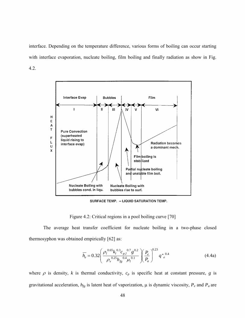
48
interface. Depending on the temperature difference, various forms of boiling can occur starting
with interface evaporation, nucleate boiling, film boiling and finally radiation as show in Fig.
4.2.
Figure 4.2: Critical regions in a pool boiling curve [70]
The average heat transfer coefficient for nucleate boiling in a two-phase closed
thermosyphon was obtained empirically [62] as:
0.230.65 0.3 0.7 0.2
, 0.4
0.25 0.4 0.10.32 ''
l l p l ee e
av fg l
k c g Ph q
Ph
(4.4a)
where is density, k is thermal conductivity, cp is specific heat at constant pressure, g is
gravitational acceleration, hfg is latent heat of vaporization, is dynamic viscosity, Pe and Pa are

49
evaporator and atmospheric pressure, q'' is the incident heat flux, and l and v stand for liquid and
vapor respectively.
Another model based on nucleate pool boiling in the working fluid pool was reported by
Rohsenow [68] as
1/3
2/3
,
1.7
1
Pr
( )
p lle
fg sf l
l v
cqh
h C
g
(4.4b)
where is the surface tension, Csf is the solid-fluid constant, taken to be 0.0154 for polished
pentane-copper combination [71], and Pr is the Prandtl number. Finally the experimental heat
transfer coefficient was obtained using
( )
avg measured
e
p e avg e
Qh
D L T T
(4.4c)
where Dp is the pipe inner diameter, Le is the evaporator length, and Qavg-measured is the heat
throughput obtained experimentally. For design purposes, the theoretical heat transfer rate at the
evaporator was quantified using Equation 4.4a and rearranged to give
50.23 30.65 0.3 0.7 0.2
, 0.6
0.25 0.4 0.10.32
l l p l ee e e sat
av fg l
k c g PQ A T T
Ph
(4.5)
Equation 4.5 was later compared with the experimental results. Detailed calculations are
presented in Appendix A.

50
4.2.2 Heat Transfer at the Condenser
Assuming no heat losses across the CTPT, the heat rate at the condenser must be equal to
the heat rate at the evaporator assuming small fin effect (Appendix A) and small radiation from
the surface. Using Nusselt and Rohsenow‟s film condensation approach [72-75], the heat transfer
coefficient at the condenser was determined to be
13 ' 4sin( )
0.943l l v l fg
c
l c sat c
g k hh
L T T
(4.6)
where is the inclination angle from the vertical, Lc is condenser length and h’fg is the modified
latent heat given as
,
,
' 1 0.68
( )
' 0.68 ( )
fg fg
p l c sat
fg
fg fg p l sat c
h h Ja
c T TJa
h
h h c T T
where Ja is Jakob number. In this design, the heat pipe is placed vertically making a 90o angle
with the horizontal reference. In another approach given by Faghri et al. [55, 76], the condenser
heat transfer coefficient was obtained in terms of the Reynolds and Nusselt numbers. Starting
with the Reynolds number (in the adiabatic section) expressed in this context by
Re( ) ( )
l
l l c fg c
w Q
D T h T
(4.7)
where w is the velocity, is the liquid film thickness and vl is the kinematic viscosity of the
liquid and using the modified Nusselt number correlation, the average heat transfer coefficient
can be rewritten in terms of the average Nusselt number as
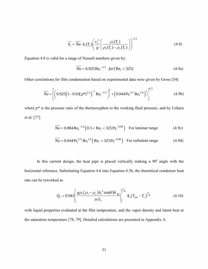
51
1/3
2 ( )( )
( ) ( )
l l cc l c
l c v c
Th Nu k T
g T T
(4.8)
Equation 4.8 is valid for a range of Nusselt numbers given by:
1/30.925Re Re 325l lNu for (4.9a)
Other correlations for film condensation based on experimental data were given by Gross [54]
1/2
21 2
3.3 1/3 2/5 1/60.925 1 0.63( *) Re 0.044Pr Rel l lNu p
(4.9b)
where p* is the pressure ratio of the thermosyphon to the working fluid pressure, and by Uehara
et al. [77]
1/4 0.960.884Re 0.5 Re 325Prl l lNu For laminar range (4.9c)
2/5 1/6 0.960.044Pr Re Re 325Prl l l lNu For turbulent range (4.9d)
In this current design, the heat pipe is placed vertically making a 90o angle with the
horizontal reference. Substituting Equation 4.6 into Equation 4.3b, the theoretical condenser heat
rate can be reworked as
13 ' 4
34
sin( )0.943
l l v l fg
c c sat c
l c
g k hQ A T T
L
(4.10)
with liquid properties evaluated at the film temperature, and the vapor density and latent heat at
the saturation temperature [78, 79]. Detailed calculations are presented in Appendix A.

52
4.2.3 Limitations of Two-Phase Thermosyphons
While closed two-phase thermosyphons (CTPTs) have worked efficiently over many
years, nevertheless, a number of restrictions are associated with the operation of these devices
that determine the maximum attainable heat transfer. Various parameters of a CTPT and the
working fluid have to be carefully selected to avoid resistance against heat transport or even
elimination of the operative mechanisms. Common limitations and the methods adopted to
overcome them are described in this section.
The viscous limit or vapor pressure limit is a constraint that influences the heat transfer
capacity when the vapor pressure at the colder side of the heat pipe approaches zero. The
saturation vapor pressure at the evaporator equalizes the pressure drop required to move the
vapor to the condenser region resulting in very low or no mass flow from the evaporator
section. This limitation occurs mainly when the CTPT is operating below the normal
operating range of the working fluid [76]. In this current design, this restriction was
eliminated by choosing the appropriate working fluids (pentane and R-134a).
The sonic limit occurs when the vapor flow velocity reaches sonic rates due to low vapor
pressure. This limit can take place at start up and during normal operation resulting in poor
function [76]. However, designing a small CTPT eliminates this limitation.
The entrainment limit is one of the most critical operation restrictions because it not only
affects the heat transfer rate, but also can cause complete burn out or destruction of the heat
pipe. Entrainment occurs when the drag force of the vapor fluid exceeds the surface tension
of the returning condensate which causes entrapment of liquid fluid with vapor. This
occurrence limits the amount of fluid that returns to the liquid pool in order to keep the heat

53
pipe cycle going and may result in dry out at the evaporator region [80]. The choice of
working fluid and its surface tension are critical in avoiding this problem.
Finally, the boiling limit and condenser limit depend on the boundary conditions and the
geometry of the ends of the CTPT [81]. The cooling rate of the condenser predicts the
maximum heat rate that can be conducted. Similarly, the input heat flux needs to be
determined correctly and accounted for in the design so that the fluid will not boil
completely.
For Proper heat pipe operation with maximum heat transfer rate, the contact surface between
the heat source and the evaporator end has to be clean at all times and free of dust to reduce
or eliminate contact resistance.
4.3 Heat Pipe Fabrication and Assembly
A wickless, gravity-assisted, closed two-phase thermosyphon (CTPT) was fabricated
with the goal of providing on demand heat transfer via a three stage process consisting of heat
acquisition, transport, and rejection in this order. The key issues associated with the design of the
CTPT are geometry, working fluid, and end boundary conditions. The CTPT geometry
incorporates cylindrical containment, an evaporator (heat source) section, and a condenser (heat
sink) section rigidly attached to form a sealed chamber. Oxygen-free high conductivity (OFHC)
copper was selected to construct the evaporator and condenser due to high thermal conductivity,
while the containment pipe was made of stainless steel to avoid corrosion and handle high
internal pressures. The lower end geometry was constructed as a flat surface with cylindrical
walls to promote uniform heating and bubble formation; and the upper end was formed with a

54
spherical shape to increase surface area and guide the liquid film condensate to flow back along
the smooth containment pipe wall. To enable expansion and contraction of the CTPT, extensible
bellows made by welding 316L SS flanges and a AM350 core were connected closer to the upper
end allowing strokes up to 4 mm from the neutral position. A schrader valve is used to allow for
the evacuation and charging of the working fluid. A schematic and picture of the assembled
CTPT with its various regions are shown in Fig. 4.3.
Figure 4.3: Assembly of the closed two-phase thermosyphon: (a) schematic with the regions A,
B, and C being the condensation, adiabatic, and evaporation regions, respectively (b) final assembly
The final heat pipe geometry such as the evaporator and condenser lengths was optimized
by iteration starting with small length values and increasing them until the heat transfer was
A
B
C
(a) (b)
C
B
A
gravity

55
maximized. This method was done using the heat transfer equations for both ends of the heat
pipe.
4.4 Thermophysical Properties of the Working Fluids
The working fluids were appropriately selected for the operation temperature and
pressure, and to avoid corrosion or gas generation due to chemical reaction with the pipe
materials. Pentane and R-134a were the working fluids selected. These working fluids were
selected based on the actuators operation temperature; however, for lunar and Mars applications,
other working fluids should be used to meet cryogenic requirements such as argon, hydrogen or
helium among other cryogens. The saturation thermophysical properties of pentane and R-134a
are shown in Tables 4.1-4 (Adopted from National Institute of Standards and Technologies
(NIST) thermophysical properties of fluid systems database).
Table 4.1: Thermophysical saturation properties for pentane (liquid phase)
Temperature
(C)
Pressure
(MPa)
Density
(l, kg/m3)
Enthalpy
(l, kJ/kg)
Cp (l,
J/g*K)
Viscosity
(l, Pa*s)
(*10^4)
Therm. Cond.
(l, W/m*K)
(*10^1)
Surf. Tension
(l, N/m)
(*10^2)
-100 9.8012E-06 735.19 -289.28 1.9777 12.504 1.6407 2.9642 -80 1.0043 E-04 717.29 -249.53 1.999 7.8523 1.5551 2.7327 -60 6.2586 E-04 699.48 -209.24 2.0327 5.5339 1.4669 2.5022 -40 2.7187 E-03 681.58 -168.14 2.0792 4.1915 1.3791 2.2732 -20 9.0283 E-03 663.44 -125.98 2.1384 3.3262 1.2935 2.0463 0 2.4448 E-02 644.87 -82.497 2.2099 2.7221 1.2111 1.822 20 5.6558 E-02 625.7 -37.459 2.2929 2.2732 1.1325 1.6009

56
Table 4.2: Thermophysical saturation properties for pentane (vapor phase)
Temperature
(oC)
Pressure
(MPa)
Density
(v, kg/m3)
Enthalpy
(v, kJ/kg)
Cp
(v, J/g*K)
Viscosity
(v, Pa*s)
(*10^6)
Therm. Cond.
(v, W/m*K)
(*10^3)
-100 9.8012E-06 4.9117E-04 166.38 1.2073 3.94 5.494 -80 1.0043 E-04 4.5131 E-03 191.18 1.2745 4.39 6.5724 -60 6.2586 E-04 2.5505 E-02 217.25 1.3416 4.86 7.7416 -40 2.7187 E-03 1.0151 E-01 244.51 1.4133 5.33 9.0236 -20 9.0283 E-03 3.119 E-01 272.89 1.4923 5.81 10.44 0 2.4448 E-02 7.8942 E-01 302.31 1.5803 6.31 12.01
20 5.6558 E-02 1.7249 332.65 1.6782 6.79 13.753
Table 4.3: Thermophysical saturation properties for R-134a (liquid phase)
Temperature
(oC)
Pressure
(MPa)
Density
(l, kg/m3)
Enthalpy
(l, kJ/kg)
Cp (l,
J/g*K)
Viscosity
(l, Pa*s)
(*10^4)
Therm. Cond.
(l, W/m*K)
(*10^1)
Surf. Tension
(l, N/m)
(*10^2)
-100 5.5914E-04 1582.4 75.362 1.1842 18.824 1.4323 2.7503 -80 3.6719 E-03 1529 99.161 1.1981 10.203 1.3154 2.4101 -60 1.5906 E-02 1474.3 123.36 1.223 6.6051 1.2071 2.0796 -40 5.1209 E-02 1417.7 148.14 1.2546 4.6703 1.1059 1.7597 -20 1.3273 E-01 1358.3 173.64 1.293 3.4758 1.0107 1.4513 0 2.928 E-01 1294.8 200 1.341 2.6653 0.92013 1.156
20 5.7171 E-01 1225.3 227.47 1.4049 2.0737 0.83284 0.87555
Table 4.4: Thermophysical saturation properties for R-134a (vapor phase)
Temperature
(oC)
Pressure
(MPa)
Density
(v, kg/m3)
Enthalpy
(v, kJ/kg)
Cp
(v, J/g*K)
Viscosity
(v, Pa*s)
(*10^6)
Therm. Cond.
(v, W/m*K)
(*10^3)
-100 5.5914E-04 0.039694 336.85 0.59322 6.96 3.3445 -80 3.6719 E-03 0.23429 348.83 0.64165 7.75 4.9479 -60 1.5906 E-02 0.92676 361.31 0.69239 8.52 6.5554 -40 5.1209 E-02 2.7695 374 0.749 9.27 8.1736 -20 1.3273 E-01 6.7845 386.55 0.8158 10 9.8164 0 2.928 E-01 14.428 398.6 0.89723 10.7 11.514 20 5.7171 E-01 27.78 409.75 1.0007 11.5 13.335
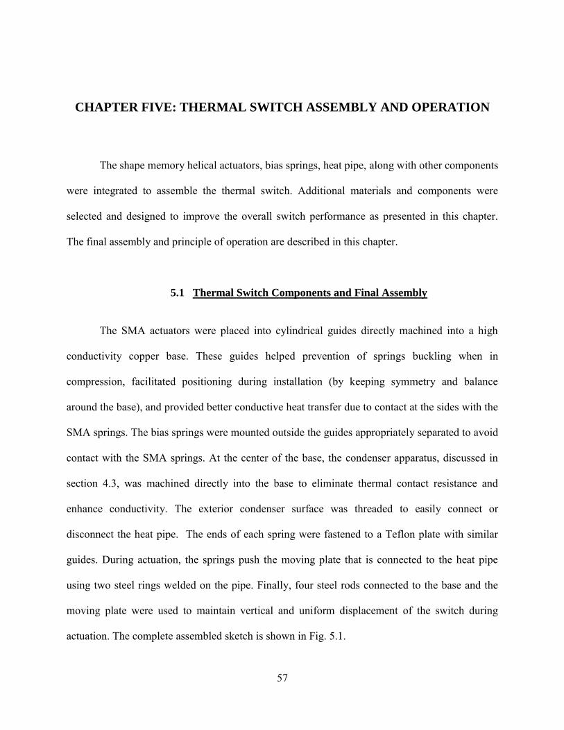
57
CHAPTER FIVE: THERMAL SWITCH ASSEMBLY AND OPERATION
The shape memory helical actuators, bias springs, heat pipe, along with other components
were integrated to assemble the thermal switch. Additional materials and components were
selected and designed to improve the overall switch performance as presented in this chapter.
The final assembly and principle of operation are described in this chapter.
5.1 Thermal Switch Components and Final Assembly
The SMA actuators were placed into cylindrical guides directly machined into a high
conductivity copper base. These guides helped prevention of springs buckling when in
compression, facilitated positioning during installation (by keeping symmetry and balance
around the base), and provided better conductive heat transfer due to contact at the sides with the
SMA springs. The bias springs were mounted outside the guides appropriately separated to avoid
contact with the SMA springs. At the center of the base, the condenser apparatus, discussed in
section 4.3, was machined directly into the base to eliminate thermal contact resistance and
enhance conductivity. The exterior condenser surface was threaded to easily connect or
disconnect the heat pipe. The ends of each spring were fastened to a Teflon plate with similar
guides. During actuation, the springs push the moving plate that is connected to the heat pipe
using two steel rings welded on the pipe. Finally, four steel rods connected to the base and the
moving plate were used to maintain vertical and uniform displacement of the switch during
actuation. The complete assembled sketch is shown in Fig. 5.1.
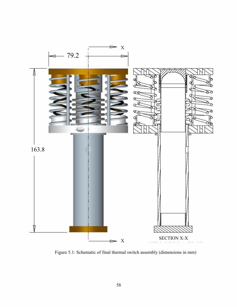
58
Figure 5.1: Schematic of final thermal switch assembly (dimensions in mm)
79.2
163.8
X
X
SECTION X-X

59
The final thermal switch assembly is shown in Fig. 5.2.
Figure 5.2: Final thermal switch assembly. The bias spring in the front was removed to show the
position of the SMA spring.
copper base and condenser
stainless steel bias spring (x4)
bellows for pipe extension
shape memory alloy actuator (x4)
Teflon (moving) plate
heat pipe containment
valve for charging fluid
evaporator (heat source)

60
5.2 Switch Operation
The objective of the thermal switch that was designed, fabricated and tested in this work
was to provide on demand heat load rejection from a liquid oxygen (LOX) tank maintained at 92
K as the temperature of the space environment varies from 40 K to 400 K on the lunar surface.
During a lunar day cycle (~14 days) when temperatures are near 400 K, the SMA springs are in
their open or “off” position and exist in their high temperature phase where they overcome the
force from the bias springs (Fig. 5.3a). In this state, the switch provides thermal isolation and no
engagement occurs. During a lunar night cycle when temperatures are near 40 K, the temperature
of the surrounding space environment drops resulting in a phase transformation in the SMA
springs. The phase transformation results in the R-phase that is now less stiffer and is overcome
by the bias springs. The resulting actuation (facilitated by bellows in the heat pipe) takes the
switch to its closed or “on” position wherein it is in thermal contact with the LOX tank (Fig.
5.3b). In this closed position, heat is rejected via conduction through the walls of the heat pipe
and by two-phase heat transfer involving the working fluid in the heat pipe. The working fluid
transfers heat in a four step process that involves: (i) fluid pool boiling at the lower (evaporator)
end due to heat addition; (ii) fluid bubble evaporation and travel; (iii) condensation of the vapor
reaching the upper (condenser) end due to the temperature drop and subsequent heat rejection;
(iv) gravity-assisted condensate flow at the condenser end; and continues to do so by repetition
of the aforementioned steps. As the temperature of the space environment increases, the SMA
actuators retract and pull the switch back to the open or “off” position recovering all the axial
displacement.

61
Figure 5.3: Principle of switch operation: (a) The open or “off” position during a lunar day (hot) (b) and the closed or “on” position during a lunar night (cold)
fluid
no heat transfer
space environment
fluid boiling
vapor
Qout
cond
ensa
te
LOX tank on lunar surface LOX tank on lunar surface Qin (a) (b)
gravity

62
CHAPTER SIX: TEST SETUP AND METHODOLOGY
A setup was built to test the final assembled thermal switch in simulated conditions. First,
an adjustable test stand was made to situate the switch in a vertical position to allow for a
complete heat transfer cycle inside the heat pipe. To simulate cryogenic conditions, liquid
nitrogen inflow and outflow lines were used to control the flow and simulate temperature
variation of the space environment that can drop to as low as 40 K. Vacuum conditions were
achieved by a glass bell jar connected to a mechanical pump and mounted on a sealed metallic
structure with instrumentation feedthroughs and valves. Auxiliary equipment such as power
supplies, heat pads, a load cell, an encoder, and thermocouples were also used for testing.
Sections of this chapter describe the test setup, methodology, instrumentation and data
acquisition using LabVIEW® virtual instruments.
6.1 Heat Pipe Evacuation and Charging
The sealed heat pipe was evacuated and charged using a high pressure manifold
connected to a mechanical pump, fluid beakers, and the valve on the thermal switch (Fig. 6.1 and
Fig. 6.2). Valves, adapters and clear flexible tubing were used to connect the manifold to the heat
pipe and charging equipment. The following scheme was used to connect the manifold lines:
Line #1: to schrader valve on heat pipe
Line #2: to fluid beaker with tube fully emerged into the liquid
Line #3: to an empty sealed beaker

63
Line #4: to mechanical pump
All other lines not used (closed valves)
The following procedure was used to charge the heat pipe:
1) Heat pipe evacuation: evacuation from one valve with all others closed
2) Evacuation of the manifold and line #3
3) Line #2 evacuation: with all valves closed, open line #3, then line #2. Due to a change
in pressure, the fluid is forced to the empty beaker filling the tubes with liquid; once
all of line # 2 is filled with liquid, close all valves.
4) Slowly open line # 1 and then line #2. The fluid flows into the pipe.
5) Weight the heat pipe before and after charging to determine the amount of fluid
transferred.
Figure 6.1: Pressure manifold for heat pipe evacuation and charging
#1 #4 #2 #3
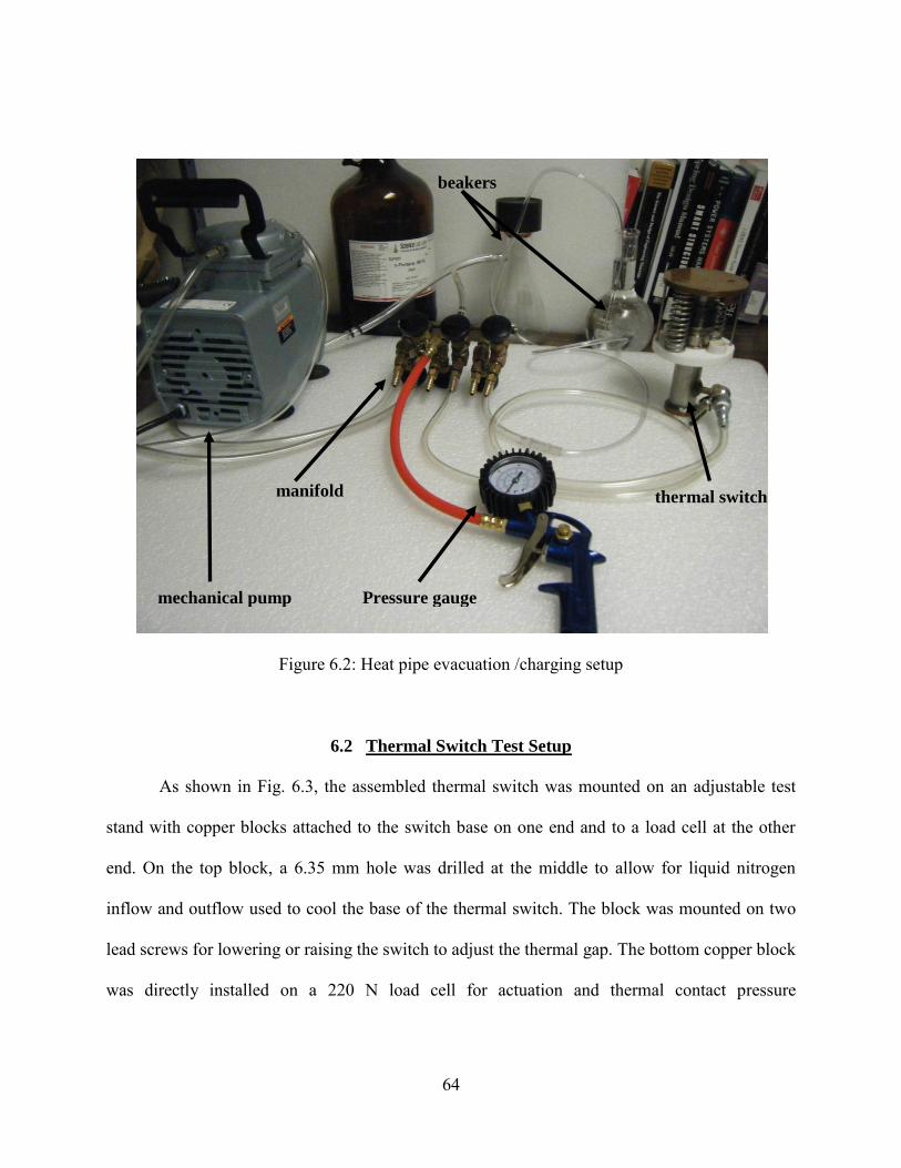
64
Figure 6.2: Heat pipe evacuation /charging setup
6.2 Thermal Switch Test Setup
As shown in Fig. 6.3, the assembled thermal switch was mounted on an adjustable test
stand with copper blocks attached to the switch base on one end and to a load cell at the other
end. On the top block, a 6.35 mm hole was drilled at the middle to allow for liquid nitrogen
inflow and outflow used to cool the base of the thermal switch. The block was mounted on two
lead screws for lowering or raising the switch to adjust the thermal gap. The bottom copper block
was directly installed on a 220 N load cell for actuation and thermal contact pressure
mechanical pump
thermal switch manifold
Pressure gauge
beakers
65
measurements. A controllable DC heat pad was placed on the lower block to control the
temperature variation during engagement of the switch.
Figure 6.3: Test stand with thermal switch: (a) schematic (b) final setup
To better control the cooling cycles, a single-loop copper tube was wrapped around the
actuators as shown in Fig. 6.4. The copper tube inlet was connected to the liquid nitrogen outlet
from the top copper block to circulate the fluid around the switch. The copper base of the switch
was put in contact with the first two loops to increase conductive cooling. During ambient tests
outside the chamber, the copper loop operates as a thermal blanket that provides forced
convective cooling for faster test runs that did not require vacuum conditions. This copper loop
was made by coiling a straight 6.35 mm copper tube around a PVC pipe with an outside diameter
(
b)
(
a)
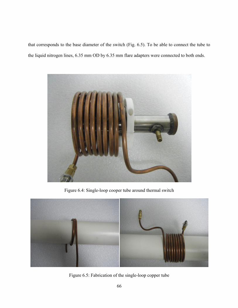
66
that corresponds to the base diameter of the switch (Fig. 6.5). To be able to connect the tube to
the liquid nitrogen lines, 6.35 mm OD by 6.35 mm flare adapters were connected to both ends.
Figure 6.4: Single-loop cooper tube around thermal switch
Figure 6.5: Fabrication of the single-loop copper tube
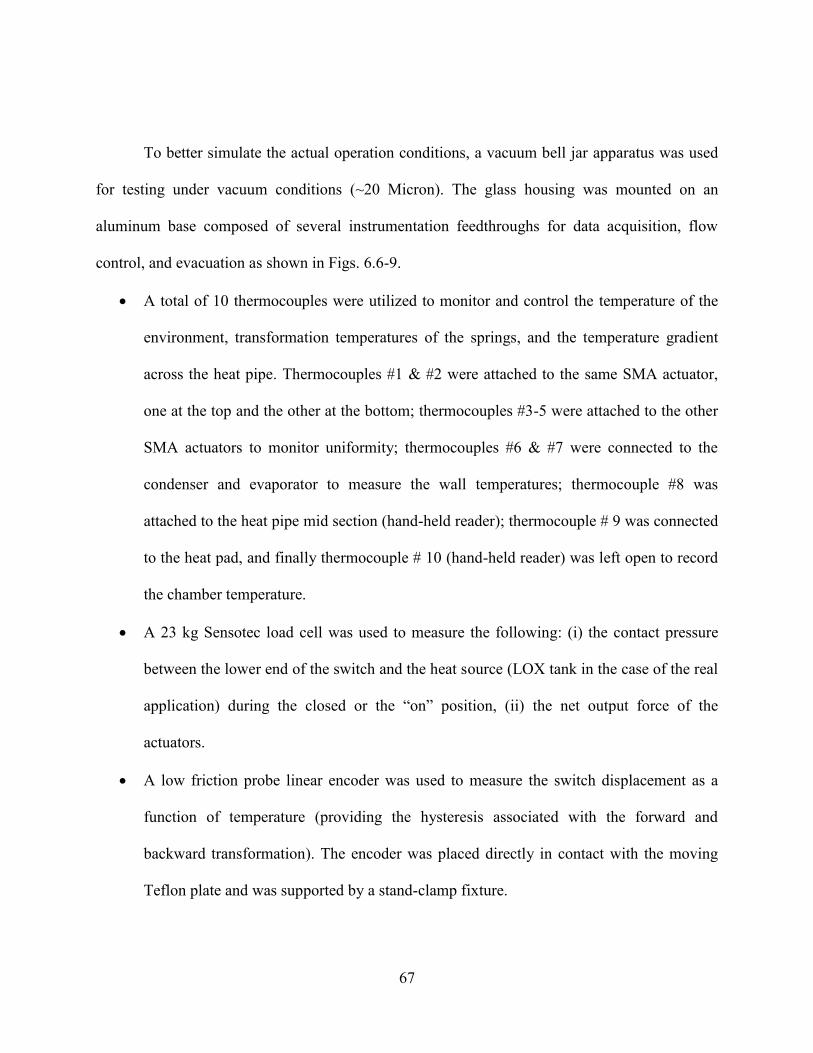
67
To better simulate the actual operation conditions, a vacuum bell jar apparatus was used
for testing under vacuum conditions (~20 Micron). The glass housing was mounted on an
aluminum base composed of several instrumentation feedthroughs for data acquisition, flow
control, and evacuation as shown in Figs. 6.6-9.
A total of 10 thermocouples were utilized to monitor and control the temperature of the
environment, transformation temperatures of the springs, and the temperature gradient
across the heat pipe. Thermocouples #1 & #2 were attached to the same SMA actuator,
one at the top and the other at the bottom; thermocouples #3-5 were attached to the other
SMA actuators to monitor uniformity; thermocouples #6 & #7 were connected to the
condenser and evaporator to measure the wall temperatures; thermocouple #8 was
attached to the heat pipe mid section (hand-held reader); thermocouple # 9 was connected
to the heat pad, and finally thermocouple # 10 (hand-held reader) was left open to record
the chamber temperature.
A 23 kg Sensotec load cell was used to measure the following: (i) the contact pressure
between the lower end of the switch and the heat source (LOX tank in the case of the real
application) during the closed or the “on” position, (ii) the net output force of the
actuators.
A low friction probe linear encoder was used to measure the switch displacement as a
function of temperature (providing the hysteresis associated with the forward and
backward transformation). The encoder was placed directly in contact with the moving
Teflon plate and was supported by a stand-clamp fixture.
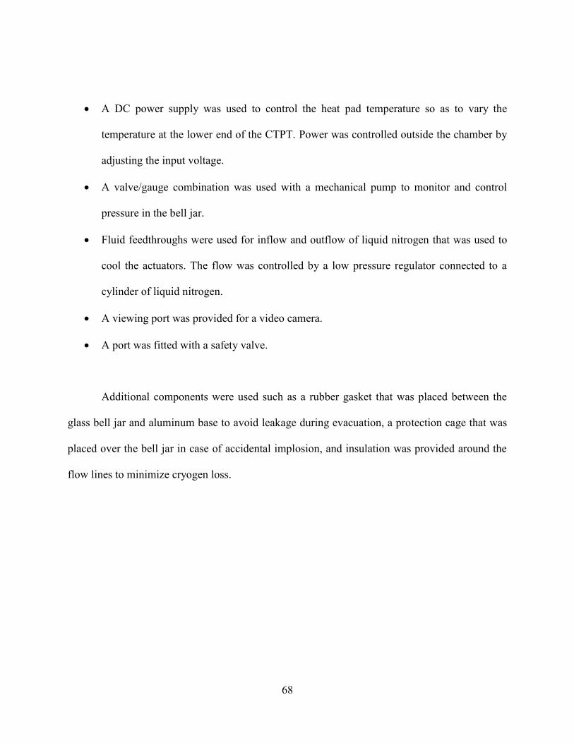
68
A DC power supply was used to control the heat pad temperature so as to vary the
temperature at the lower end of the CTPT. Power was controlled outside the chamber by
adjusting the input voltage.
A valve/gauge combination was used with a mechanical pump to monitor and control
pressure in the bell jar.
Fluid feedthroughs were used for inflow and outflow of liquid nitrogen that was used to
cool the actuators. The flow was controlled by a low pressure regulator connected to a
cylinder of liquid nitrogen.
A viewing port was provided for a video camera.
A port was fitted with a safety valve.
Additional components were used such as a rubber gasket that was placed between the
glass bell jar and aluminum base to avoid leakage during evacuation, a protection cage that was
placed over the bell jar in case of accidental implosion, and insulation was provided around the
flow lines to minimize cryogen loss.

69
Figure 6.6: Glass bell jar with instrumentation feedthroughs
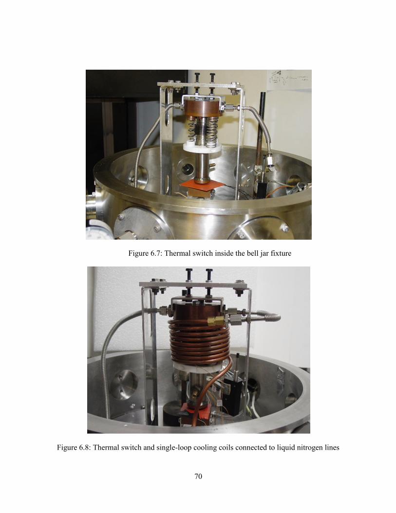
70
Figure 6.7: Thermal switch inside the bell jar fixture
Figure 6.8: Thermal switch and single-loop cooling coils connected to liquid nitrogen lines

71
Figure 6.9: Switch in instrumented vacuum bell jar setup for testing. LabVIEW® software was used for data acquisition and control of the test temperature conditions (heater and flowing liquid
nitrogen through coils).
6.3 Testing Methodology
The cooling and heating rates of the SMA actuators were determined from the
temperature-time measurements obtained from the thermocouples on the springs. These
measurements ensured that there were constant and uniform heating and cooling rates for each
spring. By adjusting the gap between the switch and the bottom block, loads and their
corresponding displacements were measured and load-stroke data thus obtained. Additionally,
thermocouples
glass jar
vacuum pump power input
liquid nitrogen flow
LabVIEW® data acquisition
switch
digital pressure gauge
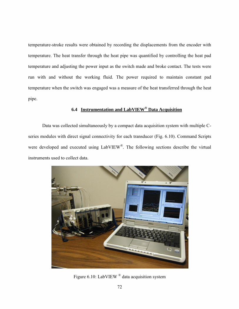
72
temperature-stroke results were obtained by recording the displacements from the encoder with
temperature. The heat transfer through the heat pipe was quantified by controlling the heat pad
temperature and adjusting the power input as the switch made and broke contact. The tests were
run with and without the working fluid. The power required to maintain constant pad
temperature when the switch was engaged was a measure of the heat transferred through the heat
pipe.
6.4 Instrumentation and LabVIEW® Data Acquisition
Data was collected simultaneously by a compact data acquisition system with multiple C-
series modules with direct signal connectivity for each transducer (Fig. 6.10). Command Scripts
were developed and executed using LabVIEW®. The following sections describe the virtual
instruments used to collect data.
Figure 6.10: LabVIEW ® data acquisition system

73
6.4.1 Temperature Virtual Instrument
The virtual instrument block diagram used to measure temperature is shown in Fig. 6.11a.
A while loop was used to continuously collect data at a specified sampling rate. A 100 ms
interval was used between measurements. Data was acquired from a total of 8 thermocouples
(denoted by TC1-8).
Figure 6.11a: Virtual instrument block diagram for temperature measurement
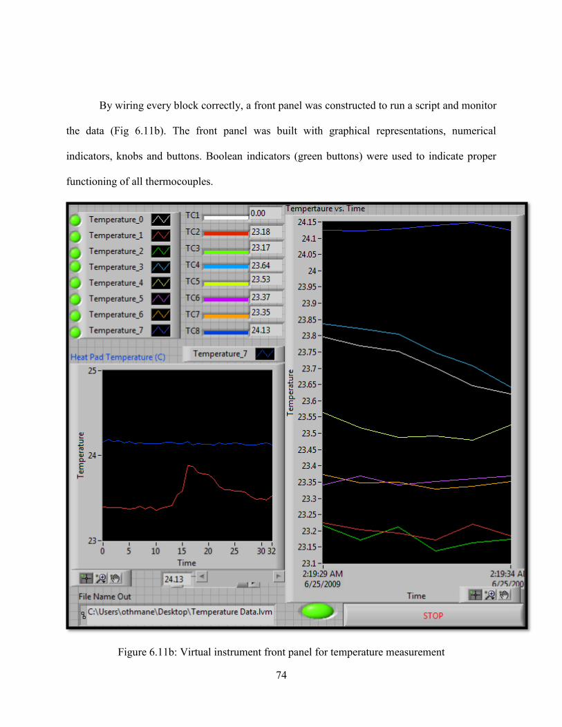
74
By wiring every block correctly, a front panel was constructed to run a script and monitor
the data (Fig 6.11b). The front panel was built with graphical representations, numerical
indicators, knobs and buttons. Boolean indicators (green buttons) were used to indicate proper
functioning of all thermocouples.
Figure 6.11b: Virtual instrument front panel for temperature measurement
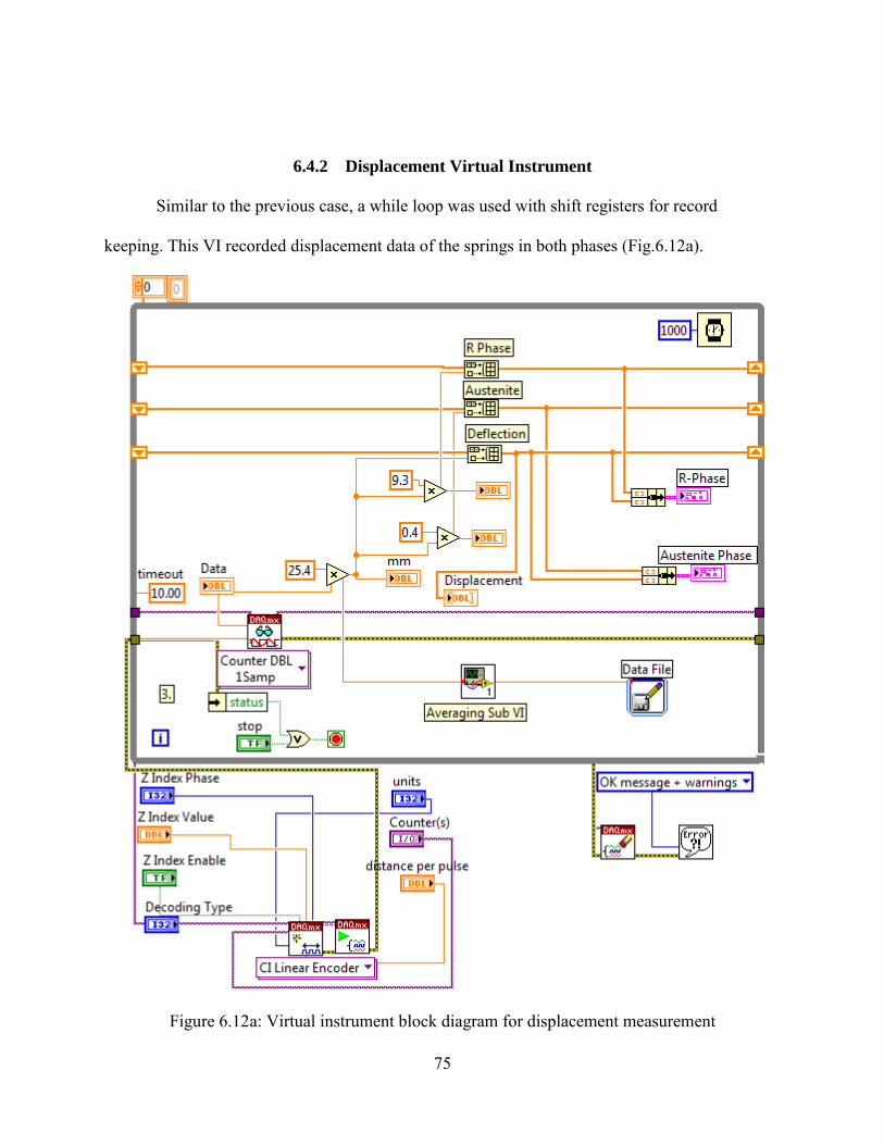
75
6.4.2 Displacement Virtual Instrument
Similar to the previous case, a while loop was used with shift registers for record
keeping. This VI recorded displacement data of the springs in both phases (Fig.6.12a).
Figure 6.12a: Virtual instrument block diagram for displacement measurement
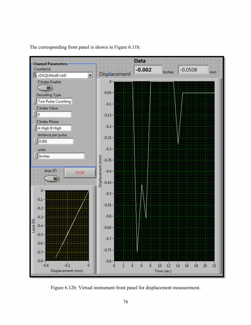
76
The corresponding front panel is shown in Figure 6.11b.
Figure 6.12b: Virtual instrument front panel for displacement measurement.
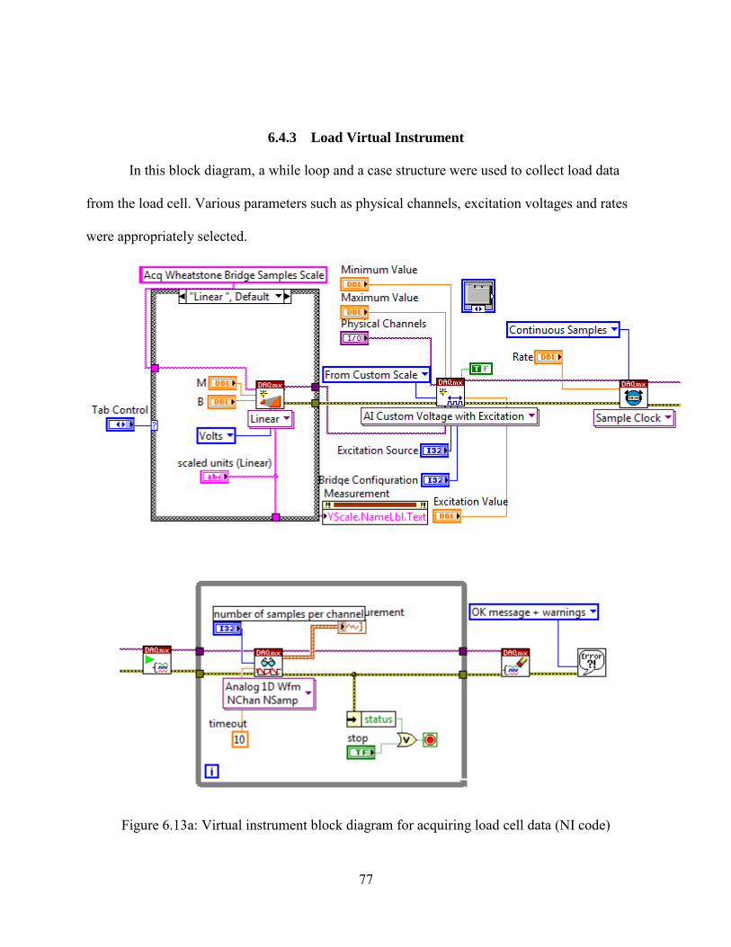
77
6.4.3 Load Virtual Instrument
In this block diagram, a while loop and a case structure were used to collect load data
from the load cell. Various parameters such as physical channels, excitation voltages and rates
were appropriately selected.
Figure 6.13a: Virtual instrument block diagram for acquiring load cell data (NI code)
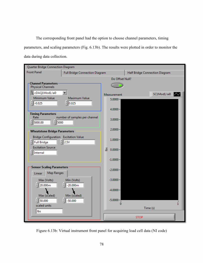
78
The corresponding front panel had the option to choose channel parameters, timing
parameters, and scaling parameters (Fig. 6.13b). The results were plotted in order to monitor the
data during data collection.
Figure 6.13b: Virtual instrument front panel for acquiring load cell data (NI code)
79
CHAPTER SEVEN: RESULTS AND DISCUSSION
This chapter presents and discusses results related to various aspects of the performance
of the shape memory actuators and the overall thermal switch.
7.1 Differential Scanning Calorimetry
The forward and reverse phase transformation temperatures for the Ni47.1Ti49.6Fe3.3 wire
used to make the springs were characterized using a Perkin Elmer Diamond differential scanning
calorimeter before and after shape setting. Samples were cut using a low speed cutting saw. The
first test was carried out to determine the transformation temperatures of the shape set wire. The
DSC curves are shown in Fig. 7.1 and reflect both the exothermic and endothermic processes
resulting from the cooling and heating cycles between 35 oC and -80 oC at a rate of 20 oC/min.
The peaks identify the start and finish of the phase transformation ( R-phase start (Rs), R-phase
finish (Rf), austenite start (As), and austenite finish (Af), respectively) during cooling followed by
heating. As mentioned previously, the R-phase exhibits a narrow transformation hysteresis as
shown by the difference in the peak temperatures (approx. 5 ºC).
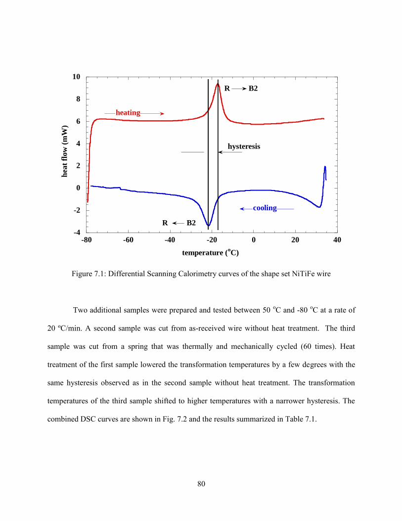
80
-4
-2
0
2
4
6
8
10
-80 -60 -40 -20 0 20 40
hea
t fl
ow
(m
W)
temperature (oC)
cooling
heating
hysteresis
B2R
B2R
Figure 7.1: Differential Scanning Calorimetry curves of the shape set NiTiFe wire
Two additional samples were prepared and tested between 50 oC and -80 oC at a rate of
20 ºC/min. A second sample was cut from as-received wire without heat treatment. The third
sample was cut from a spring that was thermally and mechanically cycled (60 times). Heat
treatment of the first sample lowered the transformation temperatures by a few degrees with the
same hysteresis observed as in the second sample without heat treatment. The transformation
temperatures of the third sample shifted to higher temperatures with a narrower hysteresis. The
combined DSC curves are shown in Fig. 7.2 and the results summarized in Table 7.1.

81
-20
-10
0
10
20
30
-80 -60 -40 -20 0 20 40
no heat treatment
shape set at 500 oC for 25 min.
shape set and cycled (60 times)
heat
flow
(m
W)
temperature (oC)
cooling
heating
Figure 7.2: DSC response of NiTiFe in the as-received, shape set and tested conditions
Table 7.1: Transformation temperatures of NiTiFe in the as-received, shape set and tested conditions.
Sample condition Rs
(oC)
Rf
(oC)
As
(oC)
Af
(oC)
Hysteresis
from peaks (oC)
No heat treatment (As received)
-10.70 -27.76 -25.15 -6.14 4.38
Shape set at 500 oC for 25 min -16.75 -28.99 -23.01 -13.44 4.71
Shape set and cycled (60 times) -9.78 -33.73 -27.74 -5.66 4.01
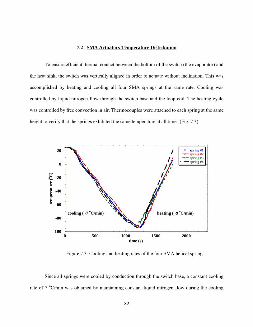
82
7.2 SMA Actuators Temperature Distribution
To ensure efficient thermal contact between the bottom of the switch (the evaporator) and
the heat sink, the switch was vertically aligned in order to actuate without inclination. This was
accomplished by heating and cooling all four SMA springs at the same rate. Cooling was
controlled by liquid nitrogen flow through the switch base and the loop coil. The heating cycle
was controlled by free convection in air. Thermocouples were attached to each spring at the same
height to verify that the springs exhibited the same temperature at all times (Fig. 7.3).
-100
-80
-60
-40
-20
0
20
0 500 1000 1500 2000
spring #1
spring #2
spring #3
spring #4
tem
pera
ture
(oC
)
time (s)
cooling (~7 oC/min) heating (~9
oC/min)
Figure 7.3: Cooling and heating rates of the four SMA helical springs
Since all springs were cooled by conduction through the switch base, a constant cooling
rate of 7 oC/min was obtained by maintaining constant liquid nitrogen flow during the cooling

83
cycle. During the convective heating cycle, a uniform heating rate of 9 oC/min was obtained. All
the springs were shown to exhibit the same temperature during a complete thermal cycle.
However, each SMA spring did not exhibit the same temperature along its length due to
conductive cooling at the upper end. To quantify the thermal gradient along the spring, three
thermocouples were attached on the same spring at different locations (points 1, 2 and 3 in Fig.
7.4). As expected, the upper section of the spring cools faster than the lower coils resulting in a
temperature gradient along the spring (Fig. 7.4). This gradient can cause an heterogeneous phase
transformation that widens the range of the transformation and the hysteresis.
-100
-80
-60
-40
-20
0
20
0 2000 4000 6000 8000
temperature @ P1
temperature @ P2
temperature @ P3
tem
per
atu
re (
oC
)
time (s)
conduction
cooling
Point 1
Point 2
Point 3
free convection
heating
Figure 7.4: Temperature distribution along the length of the SMA spring
Temperatures used to analyze and quantify the performance of the switch were reported from the
middle of the spring (Point 2).

84
7.3 Performance of the Shape Memory Alloy Helical Actuators
The experimental load-extension results associated with the actuators in the austenite and
R-phase with the bias springs are shown in Fig. 7.5 and compared with the theory (Eq. (3.6b)).
This was done in order to determine the required bias force as the SMA springs transform
between their high temperature, stiffer phase and their low temperature, more compliant phase.
The response of the high temperature phase was obtained by loading the helical actuators at
room temperature in a servo-hydraulic load frame; on the other hand, the low temperature
response was obtained while testing the switch by controlling position and measuring load. The
experimental SMA spring constants were found to be 3.72 and 0.51 N/mm for the two phases
and compared well with the theory (4.22 and 0.99 N/mm, respectively).
0
5
10
15
20
25
30
0 1 2 3 4 5 6 7
high temp. phase (theory)
high temp. phase ( experiment)low temp. phase (theory)
low temp. phase (experiment)
bias force
load
(N
)
extension (mm)
Figure 7.5: Experimental and theoretical load-extension response of the springs in the austenite
and R-phase and the bias springs

85
The results corresponding to the displacement of the switch as a function of temperature
are plotted in Fig. 7.6. Initially when in the austenite phase, the switch is maintained in the open
or “off” position providing thermal isolation. The SMA helical actuators are in their stiffer phase
and are pre-loaded with a bias force generated from the 5 mm primary compression of the bias
springs that yield a 29 N force, 4 mm pre-compression of the bellows that yield a 7.7 N force,
and from the force due to gravity of the components that exert 2.3 N. As the actuators cool and
reach the temperature for transformation from austenite to R-phase (-15.2 oC or Rs), the switch
starts to expand until -75.5 oC (Rf) following 5 mm stroke. Conversely, as the switch heats back
to room temperature, the actuators transform to the parent phase (As at -61.3 oC and Af at 3.1 oC)
concomitantly recovering all the axial deformation imposed by the bias load. The hysteresis
observed in the response is attributed to the temperature gradient along the length of the SMA
actuators. Evolution and full recovery of the phase transformation from the parent phase to R-
phase are shown in Fig. 7.6 along with the associated hysteresis. The first 3 cycles not shown
here were mainly responsible for stabilizing the material response and relieving the tensile and
compressive residual stresses at the inner and outer radii of the coil. Subsequent cycles show
consistent repeatability of the phase transformation with minimal to no open loop axial
deformation as shown in Fig. 7.7.
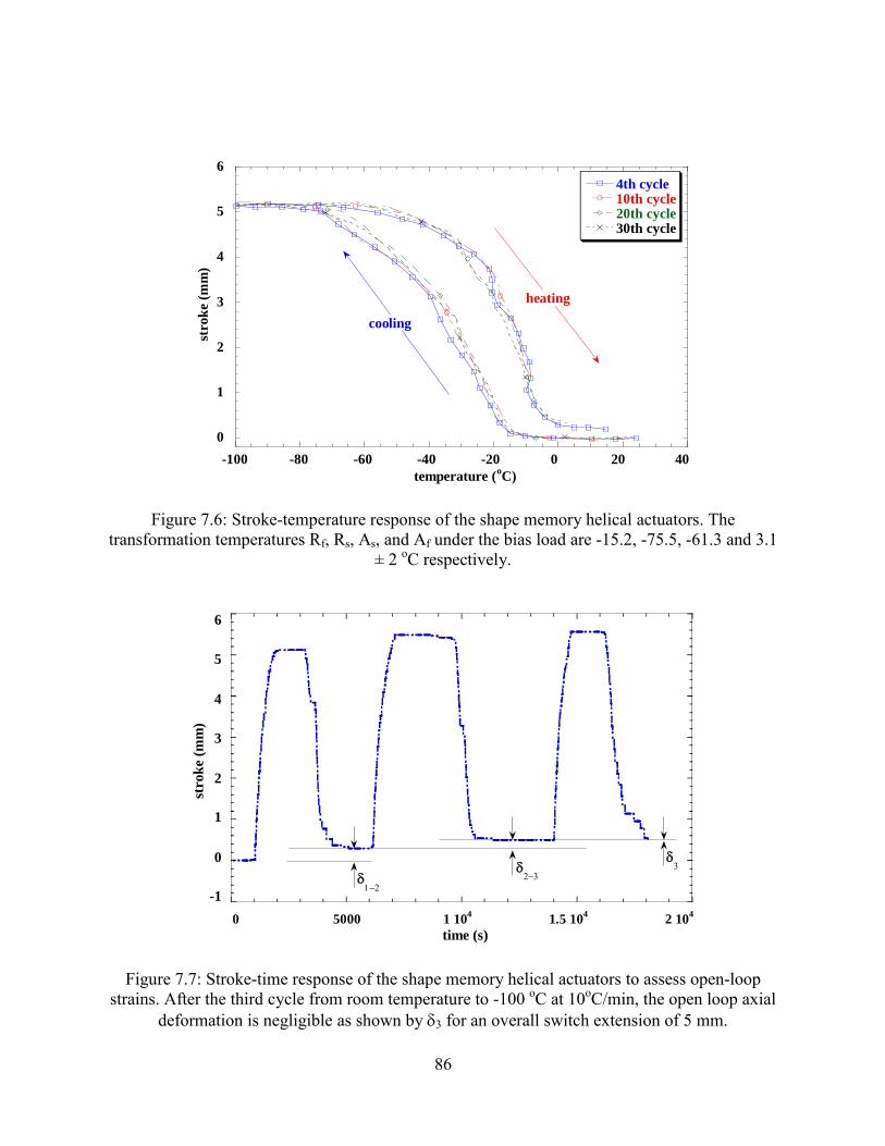
86
0
1
2
3
4
5
6
-100 -80 -60 -40 -20 0 20 40
4th cycle10th cycle20th cycle30th cycle
stro
ke (
mm
)
temperature (oC)
cooling
heating
Figure 7.6: Stroke-temperature response of the shape memory helical actuators. The transformation temperatures Rf, Rs, As, and Af under the bias load are -15.2, -75.5, -61.3 and 3.1
± 2 oC respectively.
-1
0
1
2
3
4
5
6
0 5000 1 104
1.5 104
2 104
strok
e (
mm
)
time (s)
Figure 7.7: Stroke-time response of the shape memory helical actuators to assess open-loop strains. After the third cycle from room temperature to -100 oC at 10oC/min, the open loop axial
deformation is negligible as shown by 3 for an overall switch extension of 5 mm.
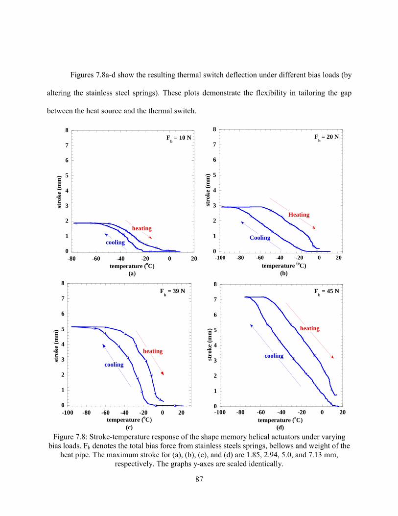
87
Figures 7.8a-d show the resulting thermal switch deflection under different bias loads (by
altering the stainless steel springs). These plots demonstrate the flexibility in tailoring the gap
between the heat source and the thermal switch.
0
1
2
3
4
5
6
7
8
-80 -60 -40 -20 0 20
stro
ke (
mm
)
temperature (oC)
(a)
Fb = 10 N
cooling
heating
0
1
2
3
4
5
6
7
8
-100 -80 -60 -40 -20 0 20
stro
ke
(mm
)
temperature (o
C)
(b)
Fb
= 20 N
Cooling
Heating
0
1
2
3
4
5
6
7
8
-100 -80 -60 -40 -20 0 20
stro
ke
(mm
)
temperature (oC)
(c)
cooling
heating
Fb = 39 N
0
1
2
3
4
5
6
7
8
-100 -80 -60 -40 -20 0 20
strok
e (m
m)
temperature (oC)
(d)
cooling
heating
Fb = 45 N
Figure 7.8: Stroke-temperature response of the shape memory helical actuators under varying
bias loads. Fb denotes the total bias force from stainless steels springs, bellows and weight of the heat pipe. The maximum stroke for (a), (b), (c), and (d) are 1.85, 2.94, 5.0, and 7.13 mm,
respectively. The graphs y-axes are scaled identically.
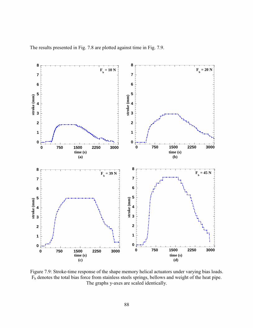
88
The results presented in Fig. 7.8 are plotted against time in Fig. 7.9.
0
1
2
3
4
5
6
7
8
0 750 1500 2250 3000
stro
ke (
mm
)
time (s)
(a)
Fb = 10 N
0
1
2
3
4
5
6
7
8
0 750 1500 2250 3000
stro
ke (
mm
)
time (s)
(b)
Fb = 20 N
0
1
2
3
4
5
6
7
8
0 750 1500 2250 3000
strok
e (m
m)
time (s)
(c)
Fb = 39 N
0
1
2
3
4
5
6
7
8
0 750 1500 2250 3000
stro
ke (
mm
)
time (s)
(d)
Fb = 45 N
Figure 7.9: Stroke-time response of the shape memory helical actuators under varying bias loads. Fb denotes the total bias force from stainless steels springs, bellows and weight of the heat pipe.
The graphs y-axes are scaled identically.
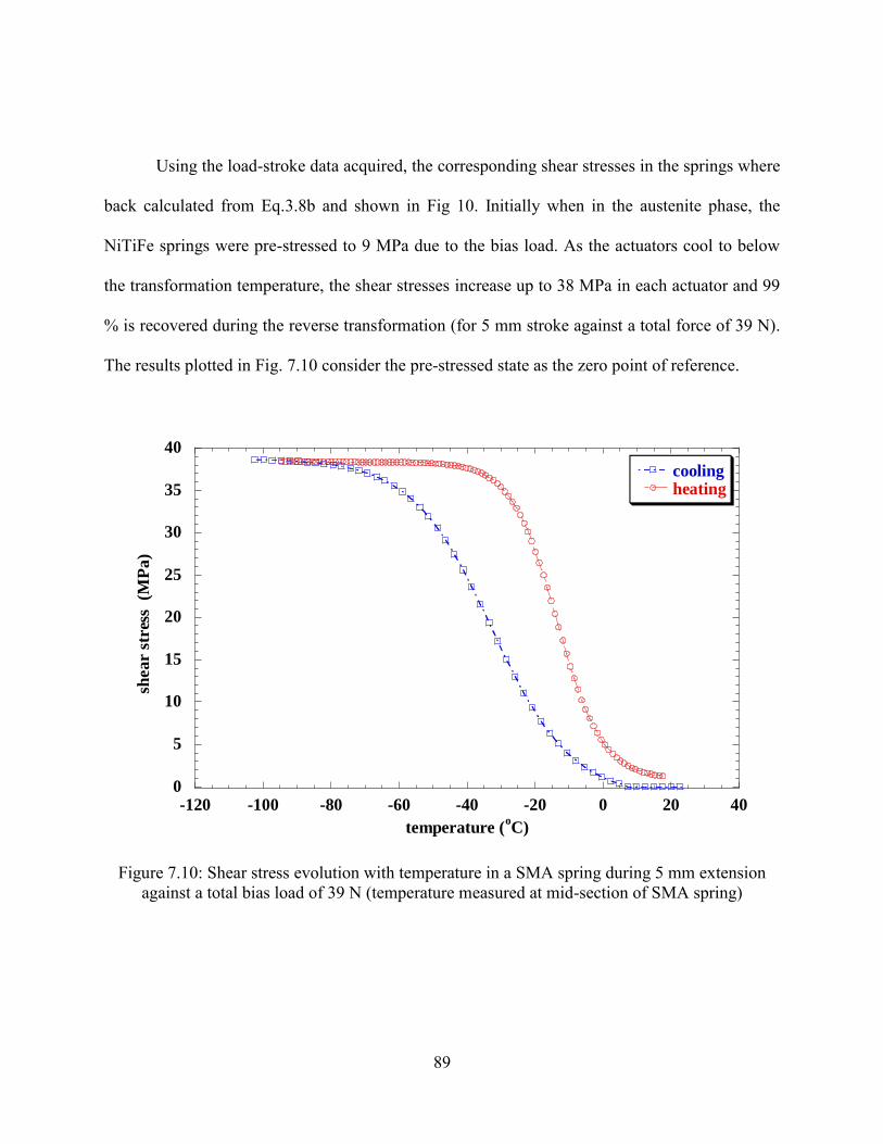
89
Using the load-stroke data acquired, the corresponding shear stresses in the springs where
back calculated from Eq.3.8b and shown in Fig 10. Initially when in the austenite phase, the
NiTiFe springs were pre-stressed to 9 MPa due to the bias load. As the actuators cool to below
the transformation temperature, the shear stresses increase up to 38 MPa in each actuator and 99
% is recovered during the reverse transformation (for 5 mm stroke against a total force of 39 N).
The results plotted in Fig. 7.10 consider the pre-stressed state as the zero point of reference.
0
5
10
15
20
25
30
35
40
-120 -100 -80 -60 -40 -20 0 20 40
coolingheating
shear s
tres
s (
MP
a)
temperature (oC)
Figure 7.10: Shear stress evolution with temperature in a SMA spring during 5 mm extension against a total bias load of 39 N (temperature measured at mid-section of SMA spring)
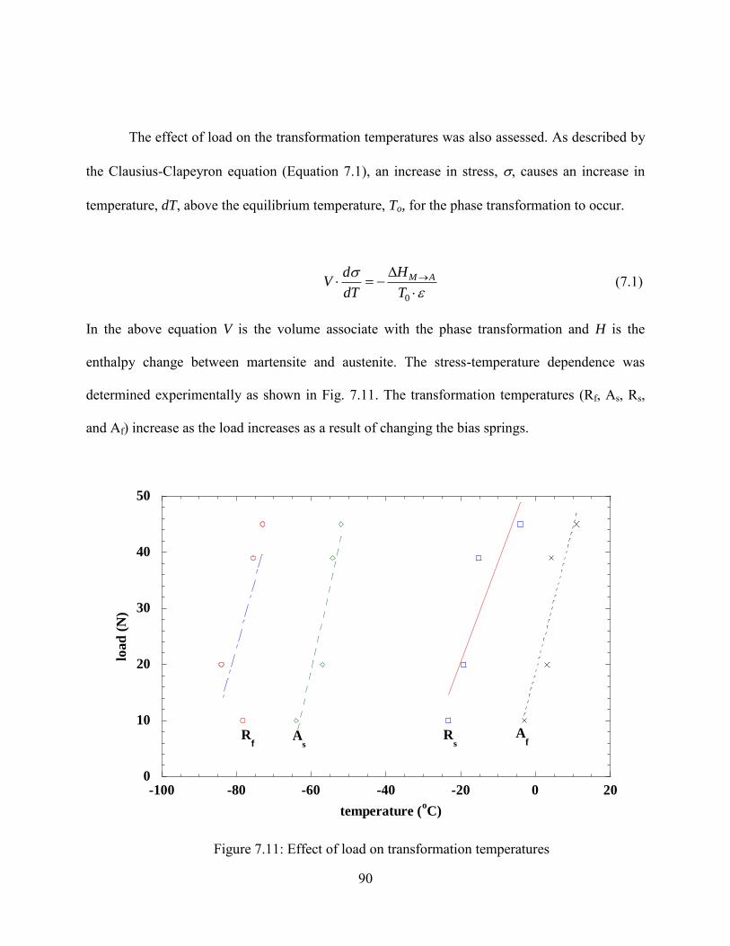
90
The effect of load on the transformation temperatures was also assessed. As described by
the Clausius-Clapeyron equation (Equation 7.1), an increase in stress, , causes an increase in
temperature, dT, above the equilibrium temperature, To, for the phase transformation to occur.
0
M AHdV
dT T
(7.1)
In the above equation V is the volume associate with the phase transformation and H is the
enthalpy change between martensite and austenite. The stress-temperature dependence was
determined experimentally as shown in Fig. 7.11. The transformation temperatures (Rf, As, Rs,
and Af) increase as the load increases as a result of changing the bias springs.
0
10
20
30
40
50
-100 -80 -60 -40 -20 0 20
load
(N
)
temperature (oC)
Rs
As
Rf
Af
Figure 7.11: Effect of load on transformation temperatures
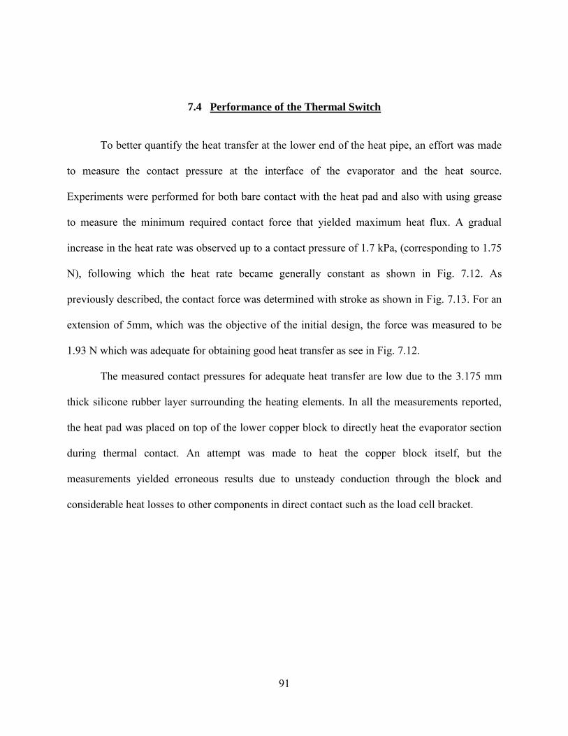
91
7.4 Performance of the Thermal Switch
To better quantify the heat transfer at the lower end of the heat pipe, an effort was made
to measure the contact pressure at the interface of the evaporator and the heat source.
Experiments were performed for both bare contact with the heat pad and also with using grease
to measure the minimum required contact force that yielded maximum heat flux. A gradual
increase in the heat rate was observed up to a contact pressure of 1.7 kPa, (corresponding to 1.75
N), following which the heat rate became generally constant as shown in Fig. 7.12. As
previously described, the contact force was determined with stroke as shown in Fig. 7.13. For an
extension of 5mm, which was the objective of the initial design, the force was measured to be
1.93 N which was adequate for obtaining good heat transfer as see in Fig. 7.12.
The measured contact pressures for adequate heat transfer are low due to the 3.175 mm
thick silicone rubber layer surrounding the heating elements. In all the measurements reported,
the heat pad was placed on top of the lower copper block to directly heat the evaporator section
during thermal contact. An attempt was made to heat the copper block itself, but the
measurements yielded erroneous results due to unsteady conduction through the block and
considerable heat losses to other components in direct contact such as the load cell bracket.
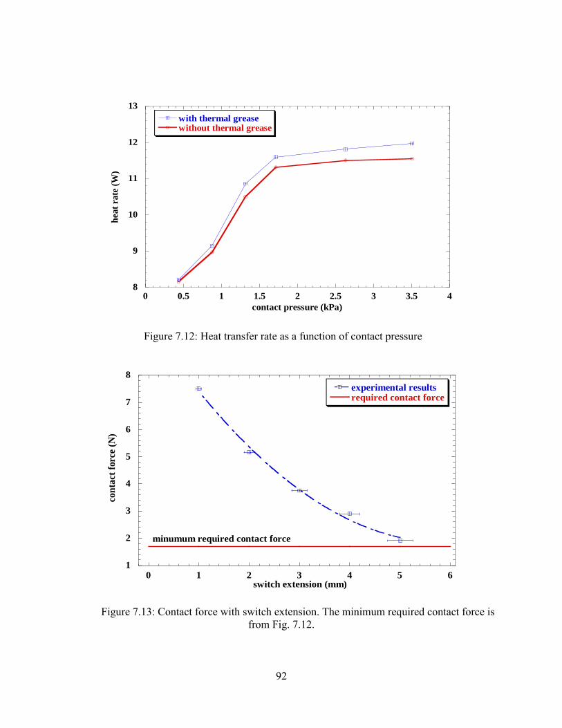
92
8
9
10
11
12
13
0 0.5 1 1.5 2 2.5 3 3.5 4
with thermal greasewithout thermal grease
hea
t ra
te (
W)
contact pressure (kPa)
Figure 7.12: Heat transfer rate as a function of contact pressure
1
2
3
4
5
6
7
8
0 1 2 3 4 5 6
experimental resultsrequired contact force
con
tact
forc
e (N
)
switch extension (mm)
minumum required contact force
Figure 7.13: Contact force with switch extension. The minimum required contact force is from Fig. 7.12.
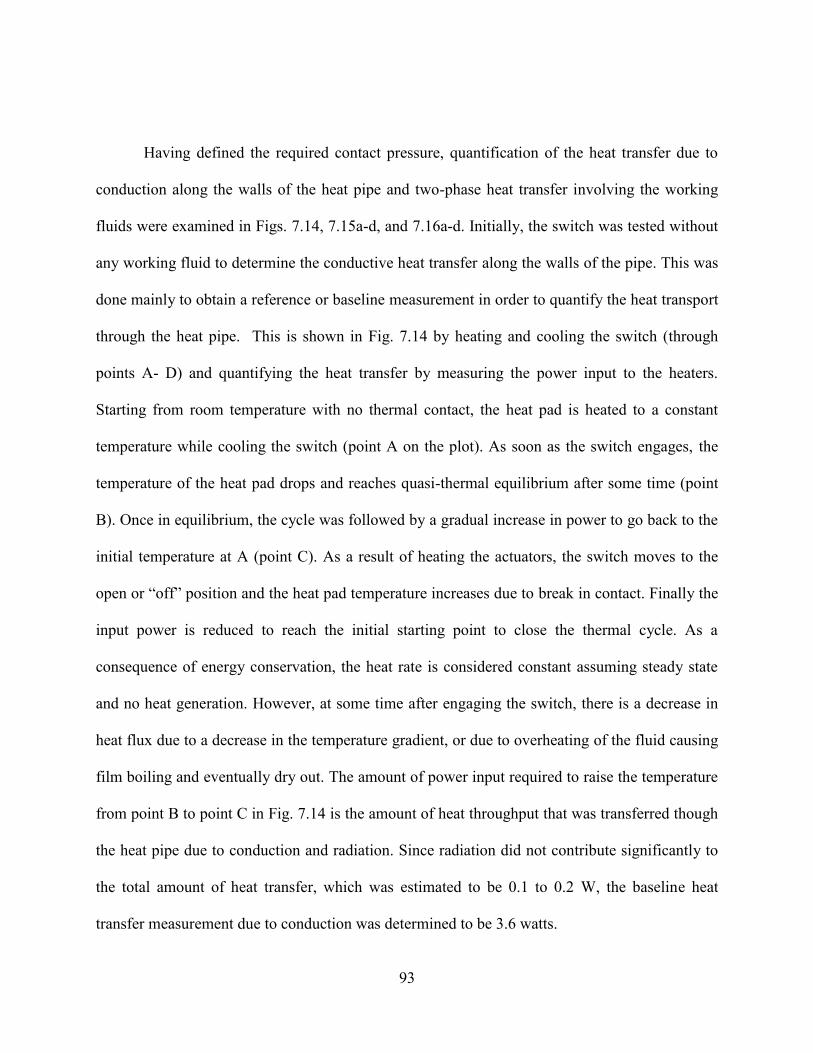
93
Having defined the required contact pressure, quantification of the heat transfer due to
conduction along the walls of the heat pipe and two-phase heat transfer involving the working
fluids were examined in Figs. 7.14, 7.15a-d, and 7.16a-d. Initially, the switch was tested without
any working fluid to determine the conductive heat transfer along the walls of the pipe. This was
done mainly to obtain a reference or baseline measurement in order to quantify the heat transport
through the heat pipe. This is shown in Fig. 7.14 by heating and cooling the switch (through
points A- D) and quantifying the heat transfer by measuring the power input to the heaters.
Starting from room temperature with no thermal contact, the heat pad is heated to a constant
temperature while cooling the switch (point A on the plot). As soon as the switch engages, the
temperature of the heat pad drops and reaches quasi-thermal equilibrium after some time (point
B). Once in equilibrium, the cycle was followed by a gradual increase in power to go back to the
initial temperature at A (point C). As a result of heating the actuators, the switch moves to the
open or “off” position and the heat pad temperature increases due to break in contact. Finally the
input power is reduced to reach the initial starting point to close the thermal cycle. As a
consequence of energy conservation, the heat rate is considered constant assuming steady state
and no heat generation. However, at some time after engaging the switch, there is a decrease in
heat flux due to a decrease in the temperature gradient, or due to overheating of the fluid causing
film boiling and eventually dry out. The amount of power input required to raise the temperature
from point B to point C in Fig. 7.14 is the amount of heat throughput that was transferred though
the heat pipe due to conduction and radiation. Since radiation did not contribute significantly to
the total amount of heat transfer, which was estimated to be 0.1 to 0.2 W, the baseline heat
transfer measurement due to conduction was determined to be 3.6 watts.
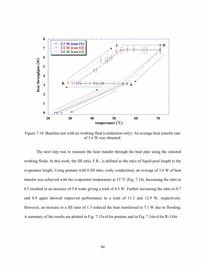
94
0
1
2
3
4
5
6
7
8
20 30 40 50 60 70
3.7 W (run #1) 3.5 W (run #2)3.6 W (run #3)
heat
thro
ug
hp
ut
(W)
temperature (oC)
AB
C D
Figure 7.14: Baseline test with no working fluid (conduction only). An average heat transfer rate of 3.6 W was obtained.
The next step was to measure the heat transfer through the heat pipe using the selected
working fluids. In this work, the fill ratio, F.R., is defined as the ratio of liquid pool length to the
evaporator length. Using pentane with 0 fill ratio, (only conduction), an average of 3.6 W of heat
transfer was achieved with the evaporator temperature at 15 oC (Fig. 7.14). Increasing the ratio to
0.5 resulted in an increase of 5.0 watts giving a total of 8.6 W. Further increasing the ratio to 0.7
and 0.9 again showed improved performance to a total of 11.3 and 12.9 W, respectively.
However, an increase to a fill ratio of 1.5 reduced the heat transferred to 7.1 W due to flooding.
A summary of the results are plotted in Fig. 7.15a-d for pentane and in Fig. 7.16a-d for R-134a.

95
0
2
4
6
8
10
12
10 20 30 40 50 60 70
Q = 8.4 Watts
Q = 8.8 Watts
Q = 8.5 Watts
heat
throu
gh
pu
t (W
)
temperature (oC)
(a)
F.R. = 50 %
0
5
10
15
0 10 20 30 40 50 60 70
Q = 11.5 Watts
Q = 11.1 Watts
Q = 11.2 Watts
hea
t th
ro
ug
hp
ut
(W)
temperature (oC)
(b)
F.R. = 70 %
0
5
10
15
20
0 10 20 30 40 50 60 70
Q = 13.0 Watts
Q = 12.7 Watts
hea
t th
rou
gh
pu
t (W
)
temperature (oC)
(c)
F.R. = 90 %
0
2
4
6
8
10
12
0 10 20 30 40 50 60 70 80
Q = 6.9 Watts
Q = 7.2 Watts
hea
t th
ro
ugh
pu
t (W
)
temperature (o
C)
(d)
F.R. = 150 %
Figure 7.15: Heat throughput using pentane: (a) F.R. = 0.5, Q = 8.6 W (b) F.R. = 0.7, Q = 11.3 W (c) F.R. = 0.9, Q = 12.9 W (d) F.R. = 1.5, Q = 7.1 W
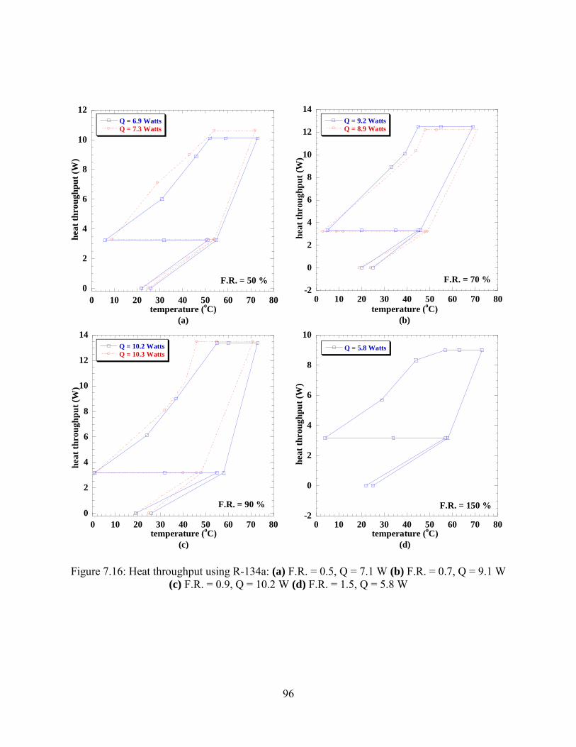
96
0
2
4
6
8
10
12
0 10 20 30 40 50 60 70 80
Q = 6.9 Watts
Q = 7.3 Watts
hea
t th
rou
gh
pu
t (W
)
temperature (oC)
(a)
F.R. = 50 %
-2
0
2
4
6
8
10
12
14
0 10 20 30 40 50 60 70 80
Q = 9.2 Watts
Q = 8.9 Watts
hea
t th
ro
ug
hp
ut
(W)
temperature (oC)
(b)
F.R. = 70 %
0
2
4
6
8
10
12
14
0 10 20 30 40 50 60 70 80
Q = 10.2 Watts
Q = 10.3 Watts
heat
throu
gh
pu
t (W
)
temperature (oC)
(c)
F.R. = 90 %
-2
0
2
4
6
8
10
0 10 20 30 40 50 60 70 80
Q = 5.8 Watts
heat
throu
gh
pu
t (W
)
temperature (oC)
(d)
F.R. = 150 %
Figure 7.16: Heat throughput using R-134a: (a) F.R. = 0.5, Q = 7.1 W (b) F.R. = 0.7, Q = 9.1 W (c) F.R. = 0.9, Q = 10.2 W (d) F.R. = 1.5, Q = 5.8 W
97
Using R-134a with 0.5 fill ratio, the average heat throughput was found to be 7.1 W.
Increasing the fill ratio to 0.7 and 0.9 increased the heat pipe performance to 9.1 and 10.2 W,
respectively. As observed in the results with pentane, increasing the fill ratio to 1.5 decreases the
heat throughput to 5.8 W. The results for R-134a are shown in Fig. 7.16. To better compare the
aforementioned heat transfer results, the heat throughputs are plotted as a function of fill ratio for
both working fluids in Fig. 7.17. Increasing the fill ratio to 1.0 increased the heat transfer for
both fluids. However, a further increase to a ratio of 1.5 showed a decrease in heat transfer due to
flooding and pressure reduction. Flooding occurs due to a large fill ratio that increases the
relative velocity between the vapor and liquid causing high interfacial viscous shear stresses that
entrain the condensate form returning back to the evaporator section.
4
6
8
10
12
14
0 0.5 1 1.5
pentane
R-134a
hea
t ra
te (
W)
fill ratio (Lf/L
e)
Figure 7.17: Heat transfer rate with fill ratio, with pentane and R-134a as working fluids in the heat pipe. Lf is the liquid pool length and Le is the length of the evaporator
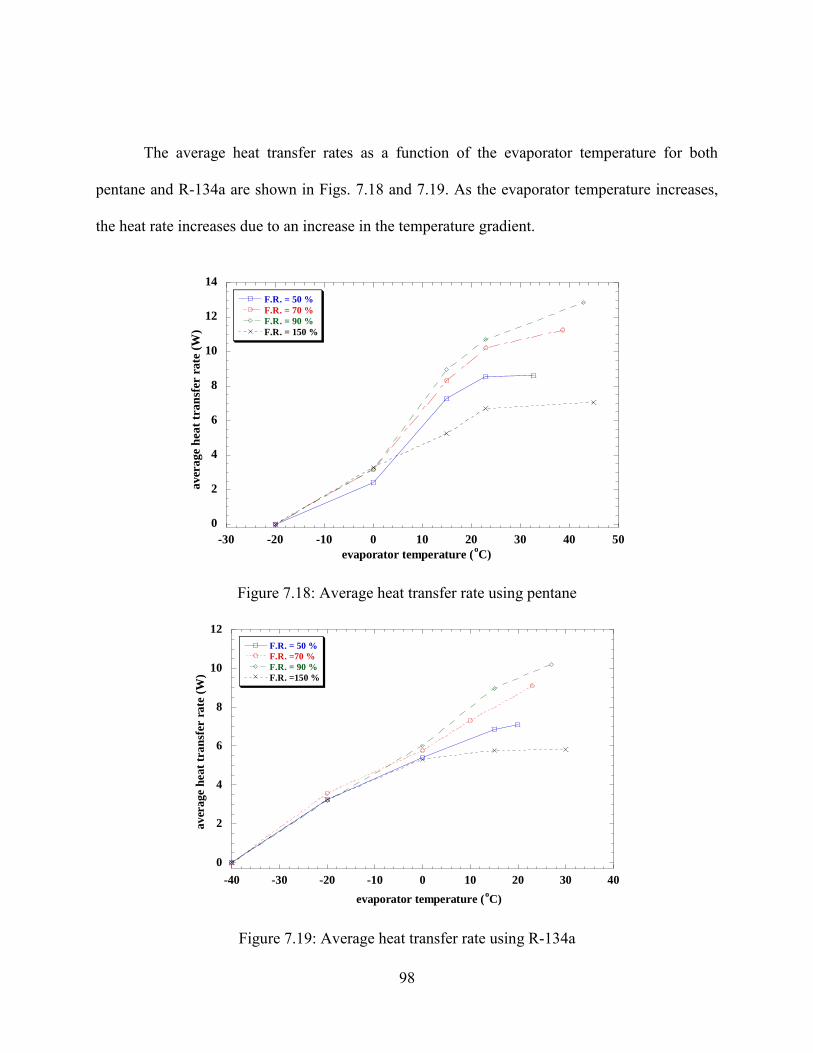
98
The average heat transfer rates as a function of the evaporator temperature for both
pentane and R-134a are shown in Figs. 7.18 and 7.19. As the evaporator temperature increases,
the heat rate increases due to an increase in the temperature gradient.
0
2
4
6
8
10
12
14
-30 -20 -10 0 10 20 30 40 50
F.R. = 50 %
F.R. = 70 %
F.R. = 90 %
F.R. = 150 %
aver
age h
ea
t tr
an
sfer
rate
(W
)
evaporator temperature (oC)
Figure 7.18: Average heat transfer rate using pentane
0
2
4
6
8
10
12
-40 -30 -20 -10 0 10 20 30 40
F.R. = 50 %
F.R. =70 %
F.R. = 90 %
F.R. =150 %
av
era
ge h
eat
tra
nsf
er r
ate
(W
)
evaporator temperature (oC)
Figure 7.19: Average heat transfer rate using R-134a

99
CHAPTER EIGHT: CONCLUSIONS AND FUTURE WORK
8.1 Conclusions
For the first time, the working of a variable length, closed two-phase heat pipe based
thermal switch incorporating low temperature helical shape memory actuators has been
presented to meet NASA‟s thermal management needs on the surface of the moon and other
advanced spaceport applications. Relevant aspects of the design, fabrication and testing
methodology for this thermal switch have been presented in detail. Such a switch integrates
sensor and actuator functions by using SMAs and does not require external sensors or actuators.
The switch can be used to: (i) enhance cryogenic handling methods for liquid and densified
cryogens and zero boil-off systems, (ii) minimize parasitic heat loads for standby cryocoolers,
(iii) control heat flow to radiators that have periodic day/night cycles (e.g., moon), and (iv) to
control heat transfer between two cryogenic storage tanks with varying heat loads (e.g., oxygen
and methane on Mars). A specific objective of this work was to assemble a switch that could
passively reject heat loads from a liquid oxygen tank at 92 K while the surrounding space
environment varies from 40 K to 400 K during the day and night cycles of the moon. The switch
was cycled between the „on‟ and „off‟ position 70 times without failure which corresponds to a
design life of 3 years in the surface of the moon. The desired life of this design is 10 years
without any downtime which can easily be met using this switch.
In terms of material selection, addition of Fe to the binary NiTi system suppressed the
martensitic transformation below room temperature and narrowed the hysteresis due to the

100
formation of a stable intermediate R-phase. This new phase offers a new temperature window for
applications that require actuation below room temperature. The NiTiFe SMA helical actuators
used in this work exhibited favorable and consistent thermo-mechanical properties while
providing a reliable passive actuation mechanism. Large stroke during transformation (up to 7
mm) against bias forces (up to 39 N) with minimal open loop axial deformation were obtained.
The actuators themselves experienced shear stresses of up to 38 MPa and recovered upwards of
99% of these stresses while cycling between low and high temperatures. Integrating these
actuators with a closed variable length two-phase heat pipe produced a thermal switch capable of
transferring up to 13 W. The valve for charging the heat pipe facilitated easy introduction of the
working fluids and two working fluids were used - pentane and R-134a.
8.2 Future Work and Recommendations
1) The NiTiFe helical actuators used in this work transform below room temperature with
transformation temperatures ranging between -15 °C and -75 °C. Applications at cryogenic
regimes cannot benefit from this alloy; hence the alloy composition has to be modified to
even lower temperatures by e.g., adding more iron in the NiTi system. Furthermore, the
thermo-mechanical properties of the SMA material can be optimized by heat treatments and
hot/cold work.
2) A large hysteresis was observed due to the temperature gradient along the length of the
spring. This can be avoided by cooling or heating the spring uniformly and not from one end
only as it is done in the current design.
101
3) The finite element analysis (FEA) performed in this work used linear elastic isotropic
properties for the alloys. It did not consider detwinning in the deformation response. An
improved model needs to be developed to capture these contributions during analyses.
4) Heat transfer analysis was based on conduction and two-phase flow heat transfer through the
heat pipe. For optimum operation, improvement is needed to better control the pipe internal
pressure and seal the pipe completely. Leakages were observed at the threaded coupling that
connected the base to the pipe. Some other mechanism could be used for rigid connection
without welding.
5) During the fluid phase change form vapor to condensate, the liquid film is returned to the
lower end assisted by gravity. For low gravity environments, a capillary wick structure
should be considered to aid the return of the liquid film to the evaporator liquid pool.
Overall, this work has laid the groundwork by demonstrating this unique thermal switch
that combines SMA actuators with a variable length heat pipe and functions without complex
external sensors or actuators. The novelty stems from the use of a low temperature, low
hysteresis NiTiFe alloy as the SMA actuator as well as successfully demonstrating its function in
a passive thermal switch by correctly accomplishing the force balance between the bellows, the
bias spring and the SMA springs. Aforementioned aspects related to optimizing material
behavior (e.g., for use at lower temperatures), heat transfer (by tailoring the mass and pressure of
the working fluid inside the heat pipe and introducing a wick if necessary) and minimizing the
gradient along the actuators can make this technology ready for practical use.

102
APPENDIX A: DESIGN CALCULATIONS

103
A-1 Spring Design Equations and Calculations
Spring design equations:
Spring constant:
Load:
Spring index:
Pitch:
Helix angle:
Spring mass:
Wire length:
SMA material properties and spring parameters:
shear modulus (austenite phase)
shear modulus (R- phase)
wire diameter
mean coil diameter
free length
maximum spring deflection
kd
4G
8 D3
Na
F k y
CD
d
pLf
Na 1
atanp
D
M Lw d
2
4
Lw DNa
cos Nia
GA 19430MPa
GR 8000MPa
dSMA 2.159mm
DSMA 15.24mm
Lf 63.5mm
ySMA 5mm
Nt 5
Nia 1

104
Calculations:
Spring index (C)
Number of active coils
Pitch (p)
Pitch angle (
Wire length (Lw)
Spring mass (M)
Spring constant (KA and KR)
CDSMA
dSMA
C 6.596
Na Nt 1 Na 3
pLf
Na 1 p 0.016m
atanp
DSMA
0.34
Lw DSMANa
cos 180Nia
Lw 0.047m
M Lw dSMA
2
4
kA 4
cos 2
GA J
sin 2
EA I
1
Na DSMA3
sec
kR 4
cos 2
GR J
sin 2
ER I
1
Na DSMA3
sec
M 1.115 103
kg
kA 4.898 103
kg
s2
kR 1.517 103
kg
s2
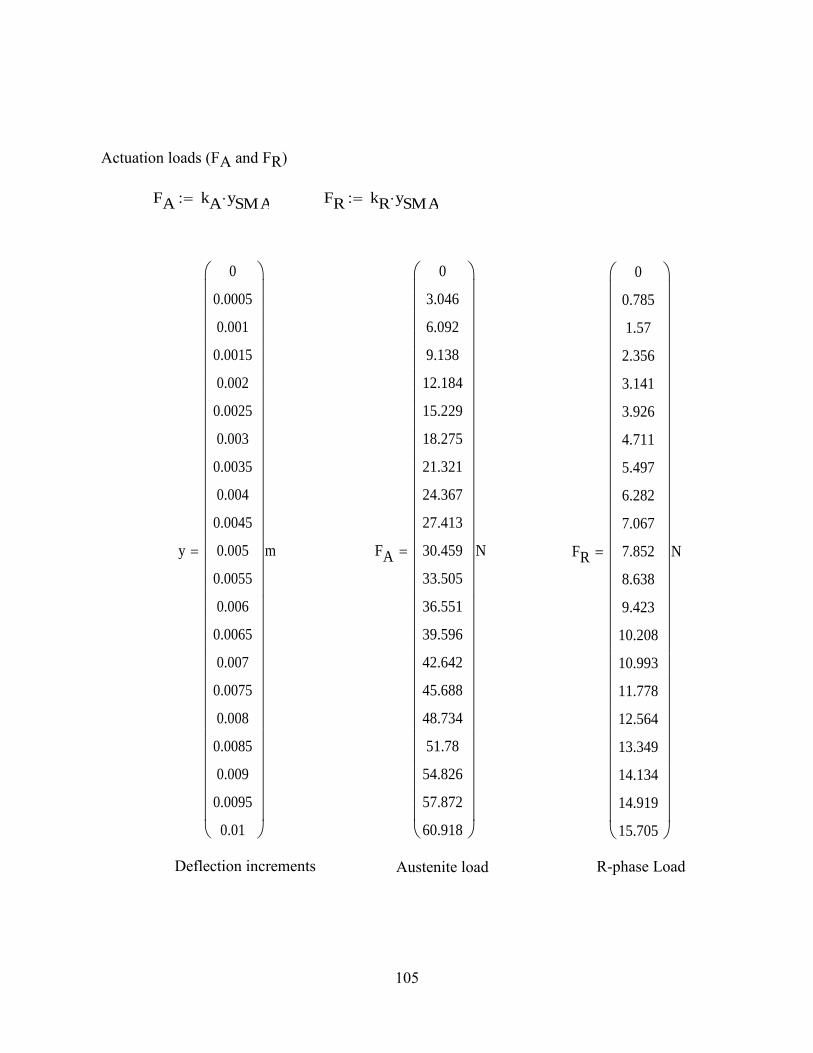
105
Actuation loads (FA and FR)
Deflection increments
R-phase Load Austenite load
FA kA ySMA FR kR ySMA
y
0
0.0005
0.001
0.0015
0.002
0.0025
0.003
0.0035
0.004
0.0045
0.005
0.0055
0.006
0.0065
0.007
0.0075
0.008
0.0085
0.009
0.0095
0.01
m FA
0
3.046
6.092
9.138
12.184
15.229
18.275
21.321
24.367
27.413
30.459
33.505
36.551
39.596
42.642
45.688
48.734
51.78
54.826
57.872
60.918
N FR
0
0.785
1.57
2.356
3.141
3.926
4.711
5.497
6.282
7.067
7.852
8.638
9.423
10.208
10.993
11.778
12.564
13.349
14.134
14.919
15.705
N
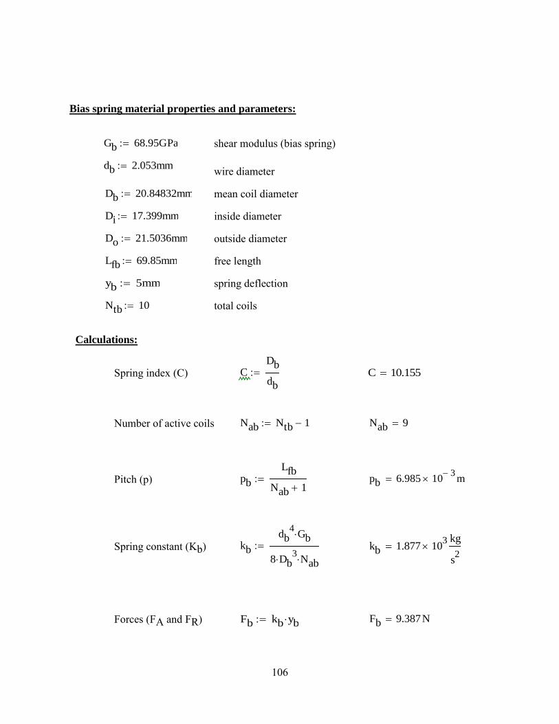
106
Bias spring material properties and parameters:
shear modulus (bias spring)
wire diameter
mean coil diameter
inside diameter
outside diameter
free length
spring deflection
total coils
Calculations:
Spring index (C)
Number of active coils
Pitch (p)
Spring constant (Kb)
Forces (FA and FR)
Gb 68.95GPa
db 2.053mm
Db 20.84832mm
Di 17.399mm
Do 21.5036mm
Lfb 69.85mm
yb 5mm
Ntb 10
CDb
db
C 10.155
Nab Ntb 1 Nab 9
pb
Lfb
Nab 1 pb 6.985 10
3 m
kb
db4
Gb
8 Db3
Nab
kb 1.877 103
kg
s2
Fb kb yb Fb 9.387N

107
SMA shear stress and shear strain:
Austenite shear stress R-phase shear stress Total shear strain
R
0
3.768 106
7.535 106
1.13 107
1.507 107
1.884 107
2.261 107
2.637 107
3.014 107
3.391 107
3.768 107
4.144 107
4.521 107
4.898 107
5.275 107
5.651 107
6.028 107
6.405 107
6.782 107
7.158 107
7.535 107
PaA
0
9.152 106
1.83 107
2.746 107
3.661 107
4.576 107
5.491 107
6.407 107
7.322 107
8.237 107
9.152 107
1.007 108
1.098 108
1.19 108
1.281 108
1.373 108
1.464 108
1.556 108
1.647 108
1.739 108
1.83 108
Pa
0
3.792 104
7.584 104
1.138 103
1.517 103
1.896 103
2.275 103
2.654 103
3.034 103
3.413 103
3.792 103
4.171 103
4.551 103
4.93 103
5.309 103
5.688 103
6.067 103
6.447 103
6.826 103
7.205 103
7.584 103

108
A-2 Comparison of SMA Spring Design Equations
Material properties:
Elastic Modulus Poisson's ratio Shear Modulus
Geometry:
wire diameter: second polar moment of area: coil diameter
# of active coils moment of area: helix angle
spring index Reduced form:
Complete form:
EA 53GPa A 0.33 GA 20GPa
ER 21GPa R 0.31 GR 8GPa
d 0.085in Jd
4
32
D 0.6in
Na 7 Id
4
64
20deg
CD
d
8Na D
3 F
GR d4
21
4Na D
3 F sec
cos 2
GR J
sin 2
ER I
38F D
3 Na
GR d4
13
16C2
3 R
2 1 R tan 2
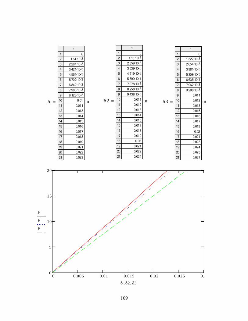
109
1
1
2
3
4
5
6
7
8
9
10
11
12
13
14
15
16
17
18
19
20
21
0
-31.14·10
-32.281·10
-33.421·10
-34.561·10
-35.702·10
-36.842·10
-37.983·10
-39.123·10
0.01
0.011
0.013
0.014
0.015
0.016
0.017
0.018
0.019
0.021
0.022
0.023
m 2
1
1
2
3
4
5
6
7
8
9
10
11
12
13
14
15
16
17
18
19
20
21
0
-31.18·10
-32.359·10
-33.539·10
-34.719·10
-35.899·10
-37.078·10
-38.258·10
-39.438·10
0.011
0.012
0.013
0.014
0.015
0.017
0.018
0.019
0.02
0.021
0.022
0.024
m 3
1
1
2
3
4
5
6
7
8
9
10
11
12
13
14
15
16
17
18
19
20
21
0
-31.327·10
-32.654·10
-33.981·10
-35.308·10
-36.635·10
-37.962·10
-39.288·10
0.011
0.012
0.013
0.015
0.016
0.017
0.019
0.02
0.021
0.023
0.024
0.025
0.027
m
0 0.005 0.01 0.015 0.02 0.025 0.030
5
10
15
20
F
F
F
2 3

110
A-3 Heat Pipe Internal Stress Analysis Equations
Axial stress
Hoop stress
Radial stress
Radial deflection
1
Pi ri2
Po ro2
ro2
ri2
2 r( )Pi ri
2 Po ro
2
ro2
ri2
ri2
ro2
Po Pi
r2
ro2
ri2
3 r( )Pi ri
2 Po ro
2
ro2
ri2
ri2
ro2
Po Pi
r2
ro2
ri2
u r( )r
E2 r( ) 3 r( ) 1

111
A-4 Heat Transfer Design Equations and Calculations (for R-134a)
R-134a properties
saturation temperature
saturation pressure
Liquid Phase Vapor Phase:
thermal conductivity
liquid Viscosity
liquid Density
enthalpy
specific Heat /p
specific Heat /v
surface tension
Heat pipe dimensions: heat pipe inner diameter
condenser length (optimized)
evaporator length (optimized)
condenser surface area
evaporator surface area
Tsat 256K
Psat 0.14989MPa
kl 0.099753W
m K kv 0.010054
W
m K
l 3.342 104 Pa s v 1.0103 10
5 Pa s
l 1349.5kg
m3
v 7.6118kg
m3
hf 177.33103
J
kg hg 388.3110
3J
kg
Cp.l 1.2992103
J
kg K Cp.v 0.8263910
3J
kg K
Cv.l 0.85842103
J
kg K Cv.v 0.7123910
3J
kg K
0.014084N
m
d 25.4mm
Lc 25.4mm
Le 50.8mm
Ac d Lc Ac 2.027 103 m
2
Ae d Le Ae 4.054 103 m
2
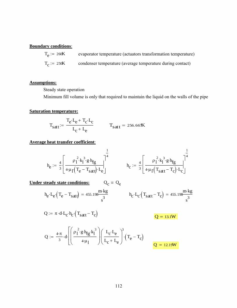
112
Boundary conditions: evaporator temperature (actuators transformation temperature)
condenser temperature (average temperature during contact)
Assumptions:
Steady state operation Minimum fill volume is only that required to maintain the liquid on the walls of the pipe
Saturation temperature:
Average heat transfer coefficient:
Under steady state conditions:
Te 260K
Tc 250K
Tsatt
Te Le Tc Lc
Lc Le Tsatt 256.667K
he4
3
l2
kl3
g hfg
4 l Te Tsatt Le
1
4
hc4
3
l2
kl3
g hfg
4 l Tsatt Tc Lc
1
4
Qc Qe
he Le Te Tsatt 455.198m kg
s3
hc Lc Tsatt Tc 455.198m kg
s3
Q d Lc hc Tsatt Tc
Q4
3d
l2
g hfg kl3
4 l
Lc Le
Lc Le
3
Te Tc 3
1
4
Q 13.1W
Q 12.19W
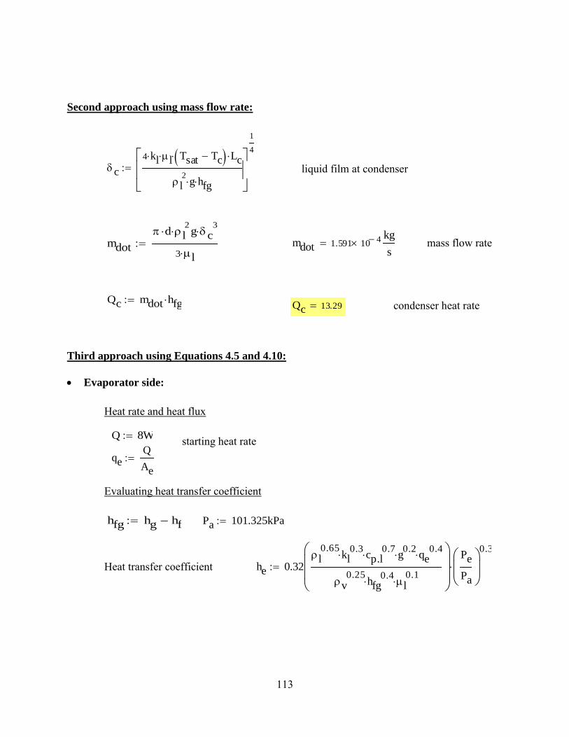
113
Second approach using mass flow rate:
Third approach using Equations 4.5 and 4.10:
Evaporator side:
liquid film at condenser
mass flow rate
condenser heat rate
Heat rate and heat flux
starting heat rate
Evaluating heat transfer coefficient
Heat transfer coefficient
c
4 kl l Tsat Tc Lc
l2
g hfg
1
4
mdot
d l2
g c3
3 l mdot 1.591 10
4kg
s
Qc mdot hfgQc 13.29
Q 8W
qeQ
Ae
hfg hg hf Pa 101.325kPa
he 0.32l
0.65kl
0.3 cp.l
0.7 g
0.2 qe
0.4
v0.25
hfg0.4
l0.1
Pe
Pa
0.3
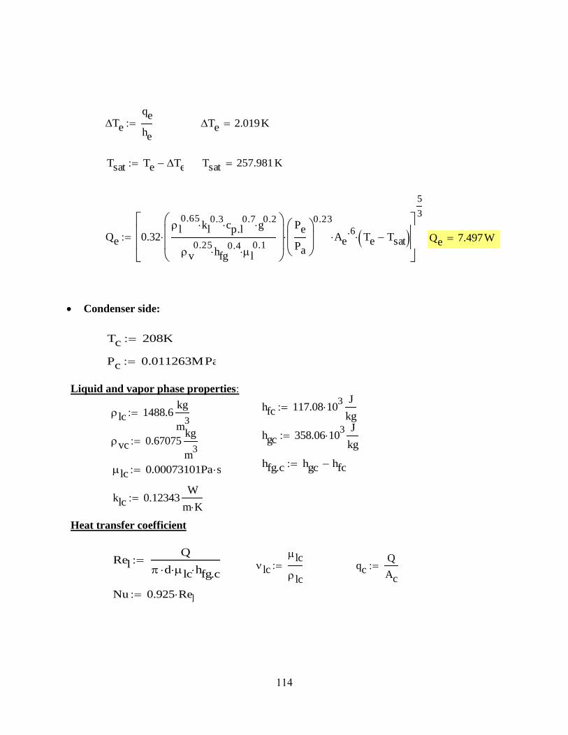
114
Condenser side:
Liquid and vapor phase properties:
Heat transfer coefficient
Te
qe
he
Te 2.019K
Tsat Te Te Tsat 257.981K
Qe 0.32l
0.65kl
0.3 cp.l
0.7 g
0.2
v0.25
hfg0.4
l0.1
Pe
Pa
0.23
Ae.6
Te Tsat
5
3
Qe 7.497W
Tc 208K
Pc 0.011263MPa
hfc 117.08 103
J
kg
lc 1488.6kg
m3
hgc 358.06 103
J
kg
vc 0.67075kg
m3
hfg.c hgc hfclc 0.00073101Pa s
klc 0.12343W
m K
RelQ
d lc hfg.c
lc
lc
lc
qcQ
Ac
Nu 0.925 Rel

115
Heat losses
hc Nu klc lc
2
g
lc
lc vc
1
3
Tc
qc
hc
Tc 1.767K
Tsatt Tc Tc Tsatt 209.767K
Qc hc Ac Tsatt Tc
Qc 7.709WQc 0.943g lc lc vc kl
3hfg.c
lc Lc
1
4
Ac Tsatt Tc
3
4
Qloss Qc QeQloss 0.212W

116
A-5 Heat Transfer Design Equations and Calculations (for Pentane)
Evaporator end:
Boundary conditions
..............................Evaporator Temperature
..............................Evaporator Pressure
Liquid and vapor phase properties
liquid density
vapor density
viscosity
enthalpy liquid
enthalpy vapor
thermal conductivity
specific Heat at constant pressure
Heat pipe dimensions
pipe inner diameter
condenser length
evaporator length
condenser area
evaporator area
Te 260K
Pe 0.012960MPa
l 657.14kg
m3
v 0.43699kg
m3
l 0.00030967Pa s
hf 111.24 103
J
kg
hg 282.86 103
J
kg
kl 0.12649W
m K
cp.l 2.1616 103
J
kg K
d 25.4mm
Lc 25.4mm
Le 50.80mm
Ac d Lc Ac 2.027 103
m2
Ae d Le Ae 4.054 103
m2
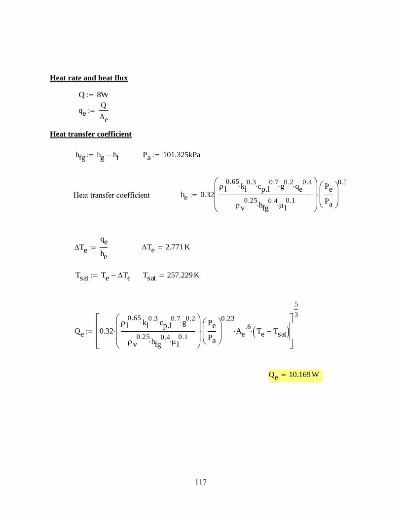
117
Heat rate and heat flux
Heat transfer coefficient
Heat transfer coefficient
Q 8W
qeQ
Ae
hfg hg hf Pa 101.325kPa
he 0.32l
0.65kl
0.3 cp.l
0.7 g
0.2 qe
0.4
v0.25
hfg0.4
l0.1
Pe
Pa
0.3
Te
qe
he
Te 2.771K
Tsat Te Te Tsat 257.229K
Qe 0.32l
0.65kl
0.3 cp.l
0.7 g
0.2
v0.25
hfg0.4
l0.1
Pe
Pa
0.23
Ae.6
Te Tsat
5
3
Qe 10.169W
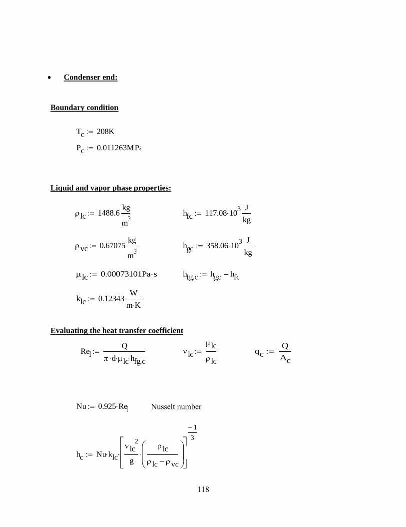
118
Condenser end:
Boundary condition
Liquid and vapor phase properties:
Evaluating the heat transfer coefficient
Nusselt number
Tc 208K
Pc 0.011263MPa
lc 1488.6kg
m3
hfc 117.08 103
J
kg
vc 0.67075kg
m3
hgc 358.06 103
J
kg
lc 0.00073101Pa s hfg.c hgc hfc
klc 0.12343W
m K
RelQ
d lc hfg.c lc
lc
lc
qcQ
Ac
Nu 0.925 Rel
hc Nu klc lc
2
g
lc
lc vc
1
3

119
Heat losses
Tc
qc
hc
Tc 1.767K
Tsatt Tc Tc Tsatt 209.767K
Qc hc Ac Tsatt Tc
Qc 0.943g lc lc vc kl
3hfg.c
lc Lc
1
4
Ac Tsatt Tc
3
4
Qc 14.314W
Qloss 4.145WQloss Qc Qe
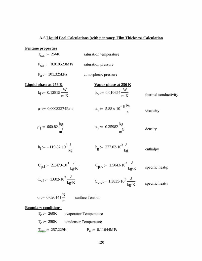
120
A-6 Liquid Pool Calculations (with pentane): Film Thickness Calculation
Pentane properties
saturation temperature
saturation pressure
atmospheric pressure
Liquid phase at 256 K Vapor phase at 256 K
thermal conductivity
viscosity
density
enthalpy
specific heat/p
specific heat/v
surface Tension
Boundary conditions: evaporator Temperature
condenser Temperature
Tsat 256K
Psat 0.010523MPa
Pa 101.325kPa
kl 0.12815W
m K kv 0.010654
W
m K
l 0.00032274Pa s v 5.88 106
Pa
s
l 660.82kg
m3
v 0.35982kg
m3
hf 119.87 103
J
kg hg 277.02 10
3
J
kg
Cp.l 2.1479 103
J
kg K Cp.v 1.5043 10
3
J
kg K
Cv.l 1.602 103
J
kg K
Cv.v 1.3835 103
J
kg K
0.020141N
m
Te 260K
Tc 250K
Tsat 257.229K Pe 0.11644MPa

121
liquid film thickness at any section
liquid film thickness at condenser section
liquid film thickness at evaporator section
Film thickness at the condenser
Film length at the evaporator section (Tf is the average temperature)
Film thickness at the evaporator
x
4 k l x Tsat Tx
hfg l l v g
0.25
c
4 k l Lc Tsat Tc
hfg l l v g
0.25
e
4 k l Lf Tf Tsat
hfg l l v g
0.25
c
4 kl l Lc Tsat Tc
hfg l l v g
0.25
c 7.733 10
5 m
Tf
Te Tsat
2 Tf 258.615K
Lf
3 Qe
d
4
3l
l2
hfg g
1
3
1
4 kl Tf Tsat
Lf 0.016m
e
4 kl l Lf Tf Tsat
hfg l l v g
0.25
e 3.852 105
m
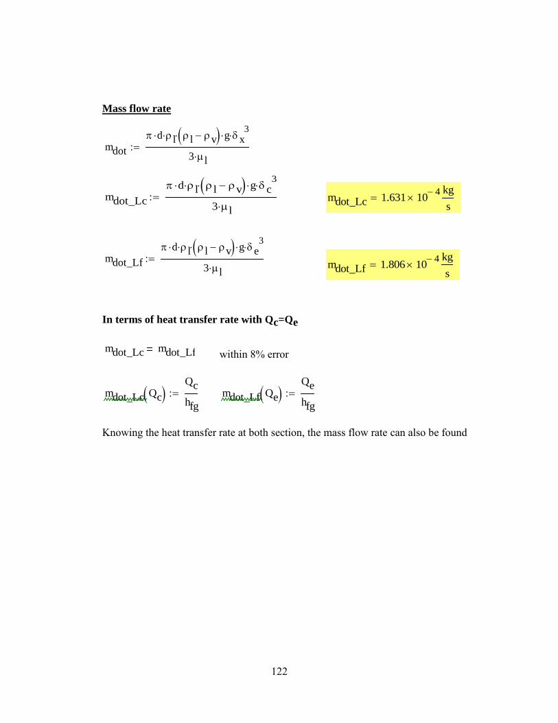
122
Mass flow rate
In terms of heat transfer rate with Qc=Qe
within 8% error
Knowing the heat transfer rate at both section, the mass flow rate can also be found
mdot
d l l v g x3
3 l
mdot_Lc
d l l v g c3
3 l mdot_Lc 1.631 10
4
kg
s
mdot_Lf
d l l v g e3
3 l
mdot_Lf 1.806 104
kg
s
mdot_Lc mdot_Lf
mdot_Lc Qc Qc
hfg
mdot_Lf Qe Qe
hfg

123
Fin Effect:
Fin effect conduction (evaporator)
Fin effect conduction (condenser)
k_copper 406W
m K
Te.s_measured 259K
Te Te Te.s_measured 2
Qf.e
Ae
Le
k_copper Te
Qf.e 1.62W
Tc.s_measured 251.2K
Tc Tc Tc.s_measured 2
Qf.c
Ae
Le
k_copper Tc
Qf.c 2.981W

124
APPENDIX B: DESIGN DRAWINGS
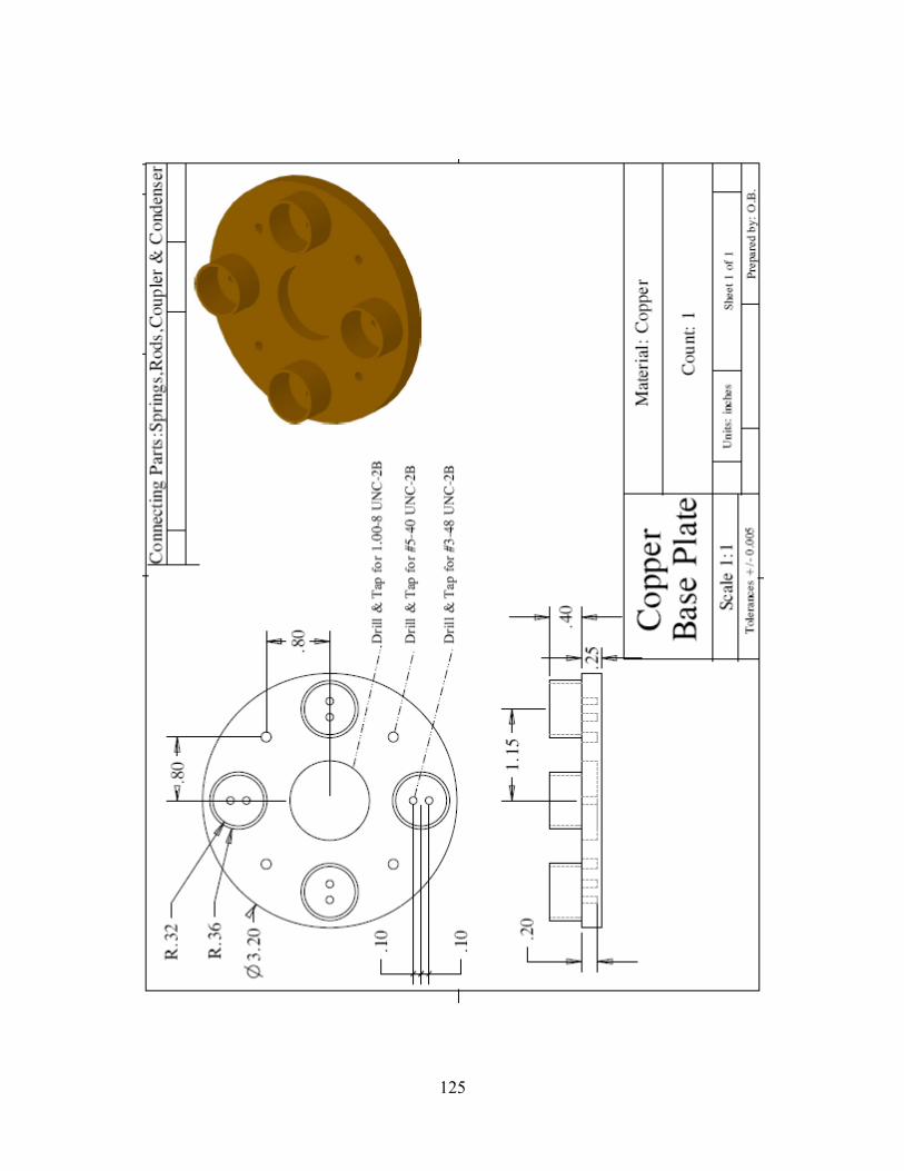
125

126

127
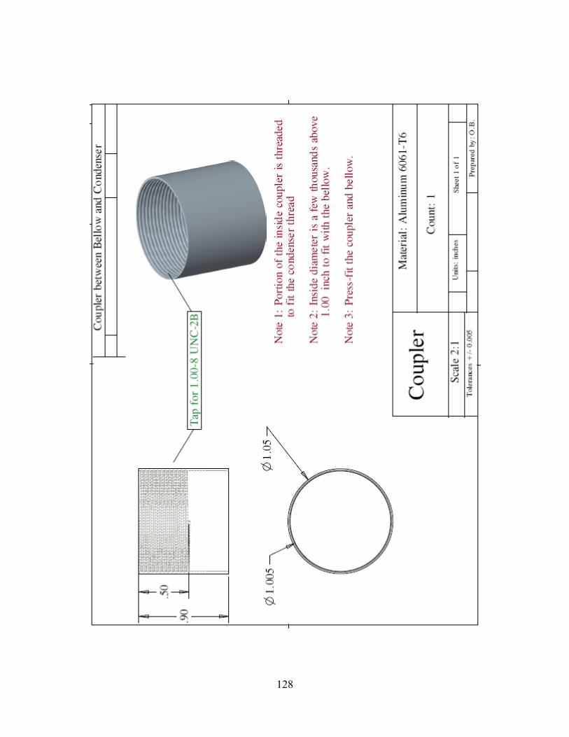
128

129

130
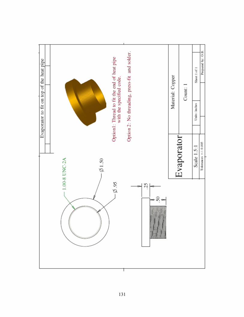
131

132
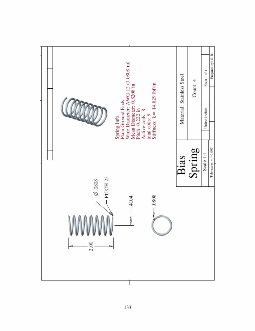
133
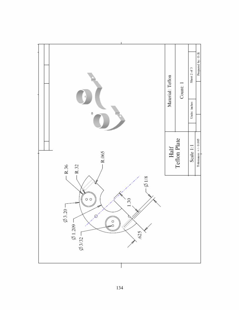
134
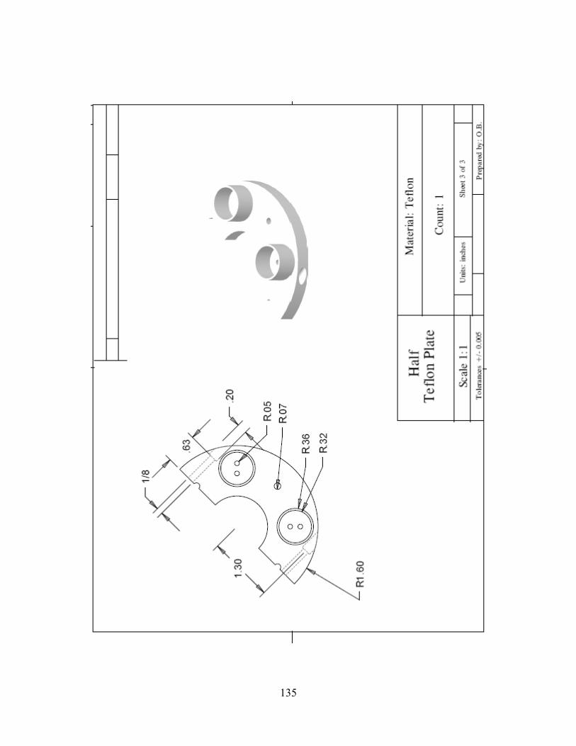
135

136
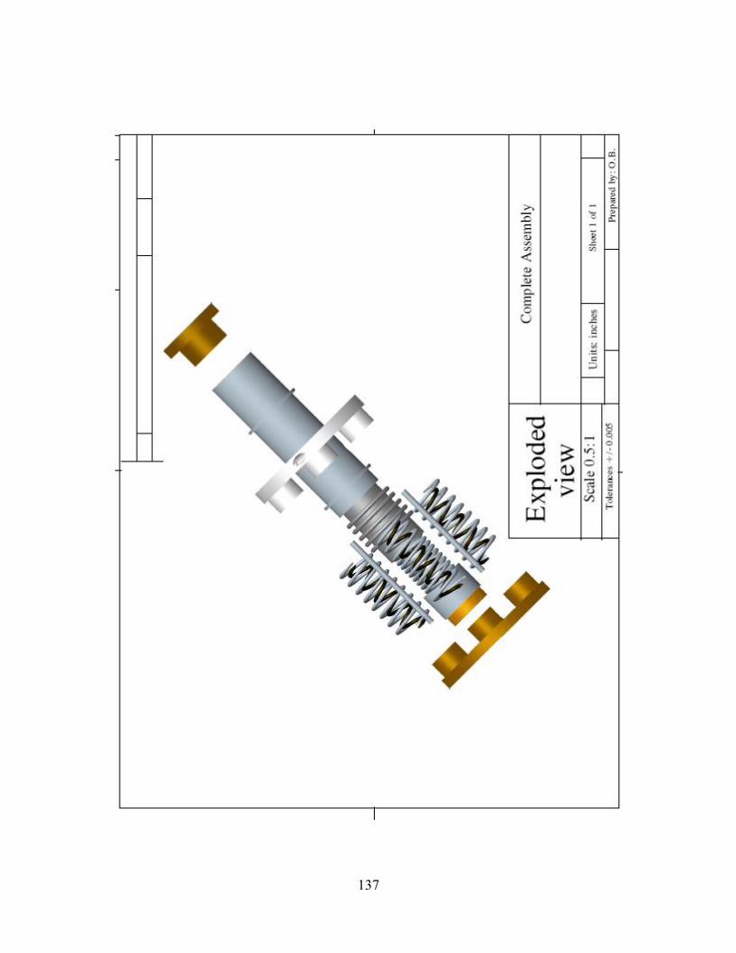
137
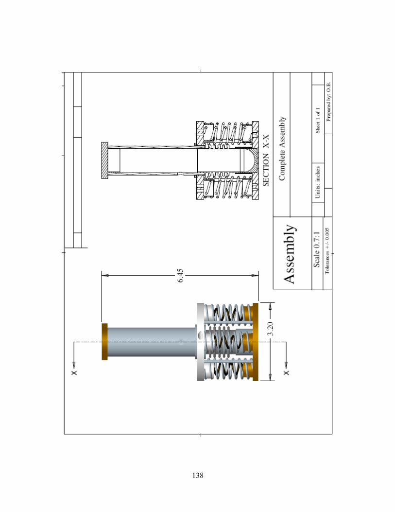
138
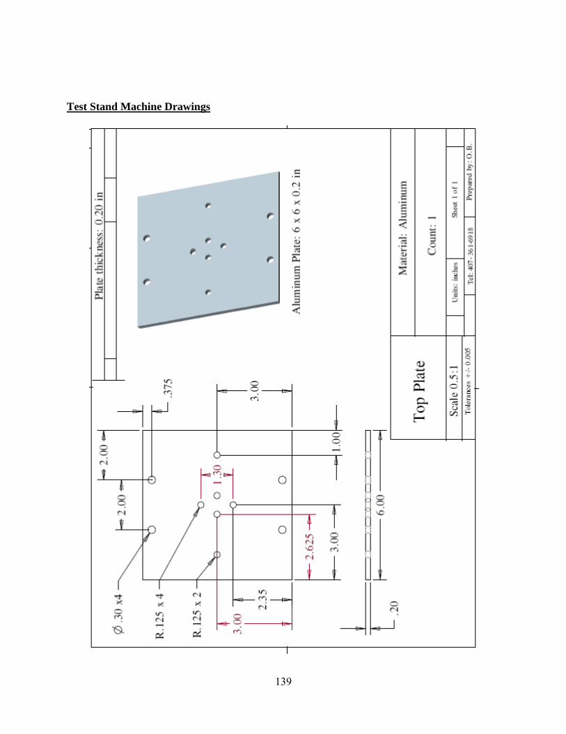
139
Test Stand Machine Drawings
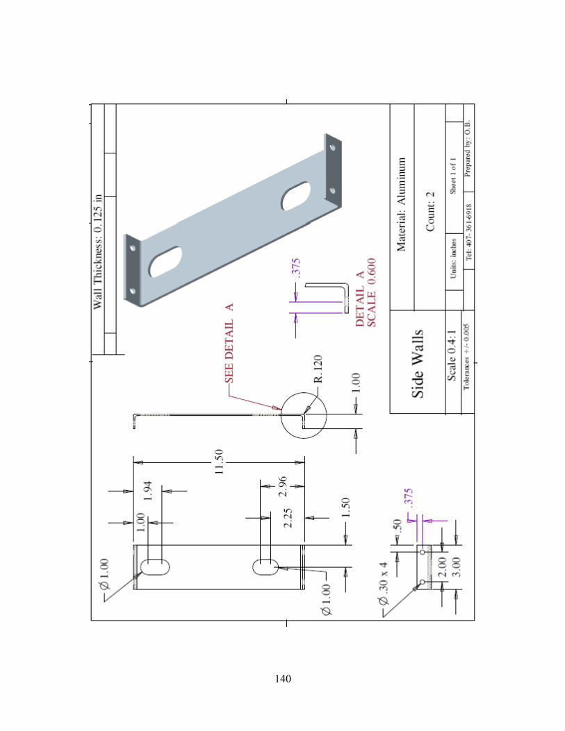
140

141
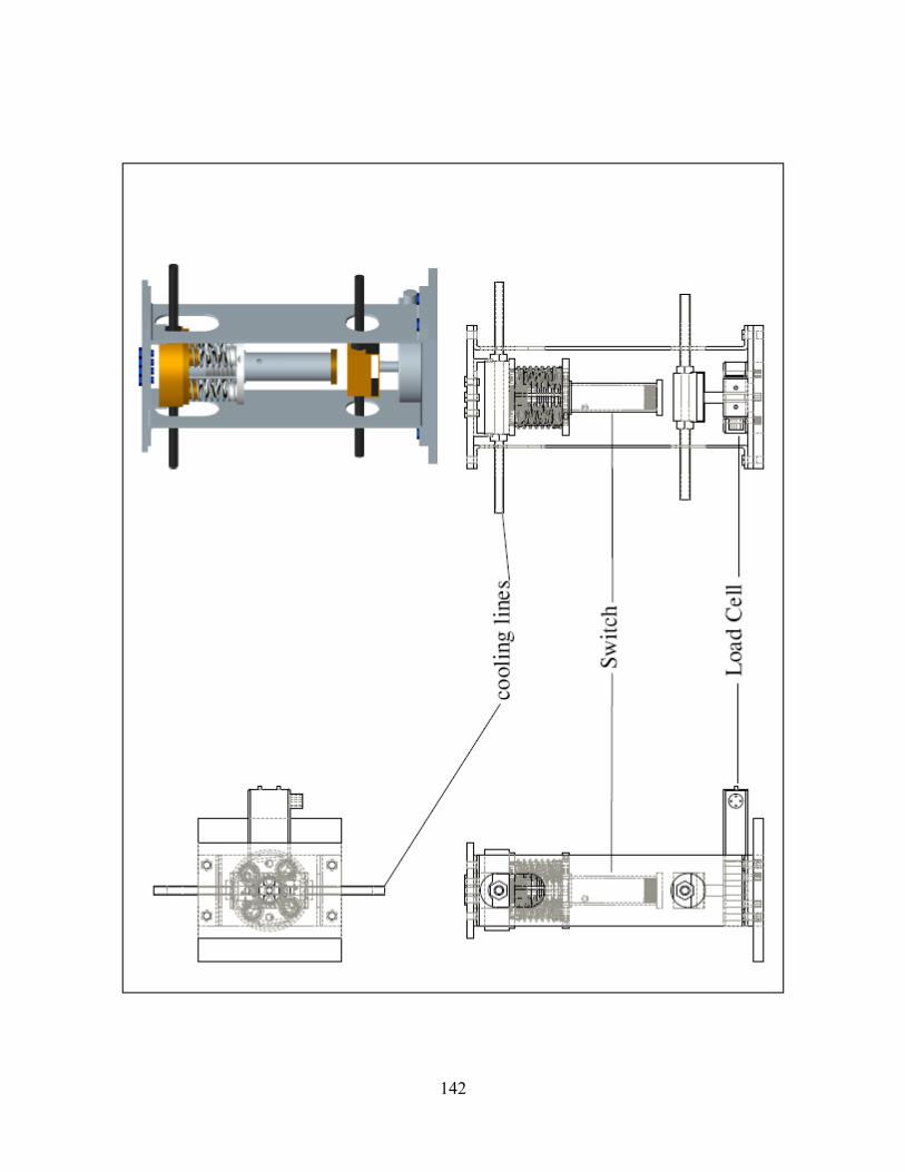
142
143
REFERENCES
[1]Donabedian M., Spacecraft Thermal Control Handbook. Cryogenics Vol. II Cryogenics. 2003, Virginia: The Aerospace Press.
[2]Duband L., A thermal switch for use at liquid helium temperature in space borne cryogenic systems. In Proc. 8th Int. Cryocooler Conf.(Colorado 1994). 1995. New York: Plenum Press.
[3]Catarino I., Bonfait G., and Duband L., Neon Gas-Gap Heat Switch. Cryogenics, 2008. 48: p.
17-25. [4]Frank D. J. and Nast T. C., Getter-activated cryogenic thermal switch. Advances in Cryogenic
Engineering, 1986. 31: p. 933-940. [5]Delaey L., et al., Review--Thermoelasticity, pseudoelasticity and the memory effects
associated with martensitic transformations--Part 2: The macroscopic mechanical behavior. Materials Science, 1974. 9: p. 1536-1544.
[6]Duerig T. W., et al., An Introduction to Martensite and Shape Memory, in Engineering
Aspects of Shape Memory Alloys. 1990, Butterworth-Heinemann: London. [7]McCormick P. G. and Y. Liu, Thermodynamic analysis of the martensitic transformation in
NiTi--II. Effect of transformation cycling. Acta Metallurgica et Materialia, 1994. 42(7): p. 2407-2413.
[8]Miyazaki S., Igo Y. and Otsuka K., Effect of thermal cycling on the transformation
temperatures of Ti---Ni alloys. Acta Metallurgica, 1986. 34(10): p. 2045-2051. [9]Otsuka K. and Ren X., Martensitic transformations in nonferrous shape memory alloys.
Materials Science and Engineering A, 1999. 273-275: p. 89-105. [10]Perkins J., et al., Thermomechanical characteristics of alloys exhibiting martensitic
thermoelasticity. Shape Memory Effects in Alloys, ed. P. J. 1976, New York: Plenum Press. [11]Funakubo H., Shape Memory Alloys. 1987, New York: Gordon and Breach. [12]Goo, E., et al., Mechanical twinning in Ti50Ni47Fe3 and Ti49Ni51 alloys. Acta
Metallurgica, 1985. 33(9): p. 1725-1733. [13]Hwang C. M., Salamon M. B. and Wayman C. M., Transformation Behaviour of a
Ti50Ni47Fe3 Alloy: III. Martensitic Transformation. Philosophical Magazine A, 1983. 47: p. 177-193.
144
[14]Hwang, C.M. and Wayman C.M., Compositional dependence of transformation temperatures in ternary TiNiAl and TiNiFe alloys. Scripta Metallurgica, 1983. 17(3): p. 381-384.
[15]Leclercq S., et al., Thermodynamical modeling of recovery stress associated with R-phase
transformation in TiNi shape memory alloys. Materials Transactions JIM, 1994. 35: p. 325-331.
[16]Miyazaki S. and Otsuka K., Deformation and transition behaviour associated with the R-
Phase in TiNi alloys. Metallurgical and Materials Transactions A, 1986. 17A: p. 53-63. [17]Krishnan, V.B., et al., Analysis of neutron diffraction spectra acquired in situ during
mechanical loading of shape memory NiTiFe at low temperatures. Materials Science and Engineering: A, 2008. 481-482: p. 3-10.
[18]Lemanski, J.L., et al., A Low Hysteresis NiTiFe Shape Memory Alloy Based Thermal
Conduction Switch. AIP Conference Proceedings, 2006. 824(1): p. 3-10. [19]Krishnan, V.B., et al., A THERMAL CONDUCTION SWITCH BASED ON LOW
HYSTERESIS NITIFE SHAPE MEMORY ALLOY HELICAL SPRINGS. AIP Conference Proceedings, 2008. 986(1): p. 3-9.
[20]Olander A., J. Amer. Soc., 1932. 54: p. 3819. [21]Greninger A. B. and Mooradian V. G., trans. AIME, 1938. 128: p. 337-341. [22]Buehler W. J. and Wang F. E., A Summary of Recent Research on the Nitinol Alloys and
their Potential Application in Ocean Engineering. Ocean Eng., 1967. 1: p. 105-120. [23]Melton K. R., ed. General applications of shape memory alloys and smart. Shape Memory
Materials, ed. Otsuka K. and Wayman C. M. 1999, Cambridge University Press: Cambridge 220-239.
[24]Schwartz M. M., New Materials Processes, and Methods Technology. 2006: Taylor and
Francis. 217-233. [25]Pitt D. M., Dunne J. P., and White E. V., Design and Test of a SMA Powered Adaptive
Aircraft Inlet Internal Wall. In 43rd AIAA/ASME/ASCE/AHS/ASC Structures, Structural Dynamics, and Materials Conference 2002. Denver, Colorado: AIAA.
[26]Mabe J. H., Calkins F., and Butler G., Boeing’s variable geometry chevron, morphing
aerostructure for jet noise reduction. In 47th AIAA/ ASME/ ASCE / AHS / ASC Structures, Structural Dynamics and Materials Conference. 1997. Newport, Rhode Island.
[27]Cross W.B., Kariotis A.H. and Stimler F.J., September1969, NASA.
145
[28]Miyazaki, S., et al., J. De Phys., 1982. 43(12). [29]Fan, G., et al., Origin of abnormal multi-stage martensitic transformation behavior in aged
Ni-rich Ti-Ni shape memory alloys. Acta Materialia, 2004. 52(14): p. 4351-4362. [30]Khalil Allafi, J., Ren X., and Eggeler G., The mechanism of multistage martensitic
transformations in aged Ni-rich NiTi shape memory alloys. Acta Materialia, 2002. 50(4): p. 793-803.
[31]Stuart R. W., Wakefield, and Hogan W. H., Thermal Switch for Cryogenic Apparatus. 1969:
USA. [32]Catarino, I., et al., Gas gap thermal switches using neon or hydrogen and sorption pump.
Vacuum, 2009. 83(10): p. 1270-1273. [33]Altoz F. E. and Porter F., Thermal Switch. 1976: USA. [34]Otsuka K. and Wayman C. M., Shape Memory Materials. 1999, Cambridge: Cambridge
University Press. p. 240-266. [35]Stebner A, et al., Development, characterization, and design consideration of
Ni19.5Ti50.5Pd25Pt5 high temperature shape memory alloy helical actuators. Journal of Intelligent Material System and structures (in print), 2009.
[36]Alghamdi S. A., A computer algorithm for the static analysis of circular helicoidal bars.
Comput. Struct, 1991. 43: p. 151-157. [37]Ancker C. J. Jr. and Goodier J. N., Theory of pitch and curvature corrections for helical
spring-I (tension). J. Appl. Mech., 1958. 25: p. 471-479. [38]Ancker C. J. Jr. and Goodier J. N., Pitch and curvature corrections for helical spring. J. Appl.
Mech., 1958. 25: p. 466-470. [39]Kamiya N. and Kita E., Boundary element method for quasi-harmonic differential equation
with application to stress analysis and shape optimization of helical springs. Comput. Struct., 1990. 37 (1): p. 81-86.
[40]Cook R. D., Finite element analysis of closely-coiled springs. Comput. Struct., 1990. 34: p.
179-180. [41]Jiang W. G. and Henshall J. L., A novel finite element for helical springs. Finite Elements
Anal. Design, 2000. 35: p. 363-377.

146
[42]Taktak M., et al., A mixed-hybrid finite element for three-dimensional isotropic helical beam analysis. Int. J. Mech. Sci., 2005. 47 (2): p. 209-229.
[43]Tautzenberger P., ed. Thermal Actuators: A Comparison of Shape Memory Alloys with
Thermostatic Bimetals and Wax Actuators. ed. Duerig T W, et al. 1990, Butterworth-Heinemann: London. 207-218.
[44]Hearn E. J., Mechanics of Materials - An Introduction to the Mechanics of Elastic and
Plastic Deformation of Solids and Structural Materials (3rd Edition). Vol. 1. 1997: Elsevier. 297-325.
[45]Wahl A. M., Mechanical Springs. 1963, New York: McGraw-Hill. [46]Hearn E. J., Mechanics of Materials - An Introduction to the Mechanics of Elastic and
Plastic Deformation of Solids and Structural Materials (3rd Edition). Vol. 1. 1997: Elsevier. 176-198.
[47]Liang C. and Rogers C. A., One-dimensional thermomechanical constitutive relations for
shape memory materials. Journal of intelligent Material System and structures 1990. 2(1). [48]Hodgson D. E., "Using Shape Memory Alloys”, Shape Memory Applications. 1988. [49]Bejan A. and Kraus A. D., Heat Transfer Handbook. 2003, NY: John Wiley & Sons. pp.
1181-1229. [50]Lock G. S. H., The Tubular Thermosyphon. 1992: Oxford University Press. [51]Lock G. S. H. and Fu, Observations on an evaporative elbow thermosyphon. Journal of Heat
Transfer, 1993. 115: p. 501-503. [52]Cheng K. C. and Zarling J. P., Applications of heat pipes and thermosyphons in cold regions.
In Proceedings of the 7th international heat pipe conference. May 1990. Minsk. [53]Harley C. and Faghri A., Complete transient two-dimensional analysis of two-phase closed
thermosyphon including the falling condensate film. Journal of Heat Transfer, 1994. 116 (2): p. 418.
[54]Gross U., Reflux Condensation heat transfer inside a closed thermosyphon. International
Journal of Heat and Mass Transfer, 1992. 35 (2): p. 279-294. [55]Faghri A., Chen M. M. and Morgan M., Heat transfer characteristic in two-phase closed
conventional and concentric annular thermosyphon Journal of Heat Transfer, 1989. 111: p. 611-618.

147
[56]Feldman K. T., Investigation of passive pressure-pumped thermosyphons. In Proceedings of the 6th international heat pipe conference. 1987. Grenoble, France.
[57]Shiraishi M., Influences of evaporator geometry on performance limits in two-phase closed thermosyphon. In Proceedings of the 6th international heat pipe conference. 1987. Grenoble, France.
[58]Shiraishi M., Yoneya M. and Yabe A., Visual study of operating limit in the two-phase
closed thermosyphon. In Proceedings of the 5th international heat pipe conference. 1984. Tokyo.
[59]Wang J.Y., et al., Performance evaluation of cell-based algorithms for domain
decomposition in flow simulation. International Journal of Numerical Methods for Heat and Fluid Flow, 2008. 18(5): p. 657-71.
[60]Tabatabai A. and Faghri A., A new two-phase flow map and transition boundary accounting
for surface tension effects in horizontal miniature and micro tubes. Journal of Heat Transfer, 2001. 123: p. 958-968.
[61]Wang J. Y. and Vafai K., An experimental investigation of the transient characteristics on a
flat plate heat pipe during startup and shutdown operations. Journal of Heat Transfer, 2000. 122: p. 525-535.
[62]Nukiyama, S., The maximum and minimum values of the heat Q transmitted from metal to
boiling water under atmospheric pressure. International Journal of Heat and Mass Transfer, 1966. 9(12): p. 1419-1433.
[63]Drew T. B. and Mueller A. C., Boiling. Transactions of AIChE, 1937. 33: p. 449-471.
[64]Yang, S. A. and Hsu C. H., Free- and forced-convection film condensation from a horizontal elliptic tube with a vertical plate and horizontal tube as special cases. International Journal of Heat and Fluid Flow, 1997. 18(6): p. 567-574.
[65]Shiraishi M., Kikuchi K., and Yamanishi T., eds. Invistigation of heat transfer
characteristics of a two-phase closed thermosyphon. Advances in Heat Pipe Thechnology, ed. Reay D A. 1981, Pergamon Press: New York. 95-103.
[66]Lee Y. and Mital U., A two-phase closed thermosyphon. International Journal of Heat and
Mass Transfer, 1972. 15(9): p. 1695-1707.
[67]Noie, S.H., Heat transfer characteristics of a two-phase closed thermosyphon. Applied Thermal Engineering, 2005. 25(4): p. 495-506.

148
[68]Rohsenow W. M., A method of correlating heat transfer data for surface boiling curves. International Journal of Heat Transfer ASME, 1962. 84: p. 969.
[69]Shalaby M. A., et al. Heat transfer performance of a two-phase closed thermosyphons. In
Proceedings of 6th International Heat Pipe Symposium. 2000. Chiang Mia.
[70]Farber E. A. and Scorah E. L., Trans. ASME, 1948. 70: p. 369.
[71]Incropera F. P., Dewitt D. P., and Bergman T L, Fundamentals of Heat and Mass Transfer. 2007: John Wiley & Sons, Inc. p.629.
[72]Nusselt W., Die oberflachen kondensation des wasserdampfes. Zeitsehrift des Vereines
Deutscher lngenieure, 1916. 60: p. 541-546.
[73]Rosenhow W. M., Heat transfer and temperature distribution in laminar-film condensation. Transactions of ASME, 1956. 78: p. 1645-1648.
[74]Collier J. G., Convective Boiling and Condensation. 1981, London: McGraw-Hill.
[75]Imura H., et al., Heat transfer in two-phase closed-type thermosyphons. Transactions of
Japan Society of Mechanical Engineers, 1977. 22: p. 485-493.
[76]Faghri A., Heat Pipe Science and Technology. 1995, Washington, DC: Taylor & Francis. 221-245.
[77]Uehara H., et al., Filmwise condensation for turbulent flow on a vertical plate. Heat Trans.-
Jpn. Res., 1983. 12((2)): p. 85-96.
[78]Sparrow E. M. and Gregg J. L., A boundary-layer treatment of laminar film condensation. Journal of Heat Transfer, 1959. 81: p. 13-18.
[79]Chen M. M., An Analytical Study of Laminar Film Condensation: Part 1- Flat Plate. Journal
of Heat Transfer, 1961. 83: p. 48-54.
[80]Dunn P D and Reay D A, The heat pipe. Physics in Technology, 1973. 4: p. 187-201.
[81]Faghri, A. and Thomas S., Performance characteristics of a concentric annular heat pipe: Part 1 - Experimental prediction and analysis of the capillary limit. Journal of Heat Transfer (Transactions of the ASME) 1989. 111(4): p. 844-850.