Design and Analysis of a Three Degrees of Freedom (DOF) Parallel Manipulator with

Decoupled Motions

by

Jijie Qian

A Thesis Submitted in Partial Fulfillment of the Requirements for the Degree of

Master of Applied Science

in

The Faculty of Engineering and Applied Science

Mechanical Engineering

University of Ontario Institute of Technology

April 2009

© Jijie Qian, 2009

CERTIFICATE OF APPROVAL Submitted by: Jijie Qian Student #: 100333621 In partial fulfillment of the requirements for the degree of: Master of Applied Science in Mechanical Engineering Date of Defense (if applicable): April 7, 2009 Thesis Title: Design and Analysis of a Three Degrees of Freedom (DOF) Parallel Manipulator with Decoupled Motions The undersigned certify that they recommend this thesis to the Office of Graduate Studies for acceptance: ____________________________ ______________________________ _______________ Chair of Examining Committee Signature Date (yyyy/mm/dd) ____________________________ ______________________________ _______________ External Examiner Signature Date (yyyy/mm/dd) ___________________________ ______________________________ _______________ Member of Examining Committee Signature Date (yyyy/mm/dd) ____________________________ ______________________________ _______________ Member of Examining Committee Signature Date (yyyy/mm/dd) As research supervisor for the above student, I certify that I have read the following defended thesis, have approved changes required by the final examiners, and recommend it to the Office of Graduate Studies for acceptance: Prof. Dan Zhang _________________________________ _______________ Name of Research Supervisor Signature of Research Supervisor Date (yyyy/mm/dd)

- ii -

Abstract

Parallel manipulators have been the subject of study of much robotic research

during the past three decades. A parallel manipulator typically consists of a moving

platform that is connected to a fixed base by at least two kinematic chains in parallel.

Parallel manipulators can provide several attractive advantages over their serial

counterpart in terms of high stiffness, high accuracy, and low inertia, which enable them

to become viable alternatives for wide applications. But parallel manipulators also have

some disadvantages, such as complex forward kinematics, small workspace, complicated

structures, and a high cost. To overcome the above shortcomings, progress on the

development of parallel manipulators with less than 6-DOF has been accelerated.

However, most of presented parallel manipulators have coupled motion between

the position and orientation of the end-effector. Therefore, the kinematic model is

complex and the manipulator is difficult to control.

Only recently, research on parallel manipulators with less than six degrees of

freedom has been leaning toward the decoupling of the position and orientation of

the end-effector, and this has really interested scientists in the area of parallel

robotics. Kinematic decoupling for a parallel manipulator is that one motion of the up-

platform only corresponds to input of one leg or one group of legs. And the input

cannot produce other motions.

Nevertheless, to date, the number of real applications of decoupled motion

actuated parallel manipulators is still quite limited. This is partially because effective

development strategies of such types of closed-loop structures are not so obvious. In

- iii -

addition, it is very difficult to design mechanisms with complete decoupling, but it is

possible for fewer DOF parallel manipulators. To realize kinematic decoupling, the

parallel manipulators are needed to possess special structures; therefore, investigating a

parallel manipulator with decoupling motion remains a challenging task.

This thesis deals with lower mobility parallel manipulator with decoupled motions.

A novel parallel manipulator is proposed in this thesis. The manipulator consists of a

moving platform that is connecting to a fixed base by three legs. Each leg is made of one

C (cylinder), one R (revolute) and one U (universal) joints. The mobility of the

manipulator and structure of the inactive joint are analyzed. Kinematics of the

manipulator including inverse and forward kinematics, velocity equation, kinematic

singularities, and stiffness are studied. The workspace of the parallel manipulator is

examined. A design optimization is conducted with the prescribed workspace.

It has been found that due to the special arrangement of the legs and joints, this

parallel manipulator performs three translational degrees of freedom with decoupled

motions, and is fully isotropic. This advantage has great potential for machine tools and

Coordinate Measuring Machine (CMM).

Keywords

Parallel manipulator; Decoupled motion; Screw theory; Isotropy; Inverse

kinematic; Forward kinematic; Jacobian; Singularity; Stiffness; Workspace; Optimization.

- iv -

Dedication

To my wife Ying, my daughter Casey and my parents.

- v -

Acknowledgments

First, I would like to express my deepest gratitude to my supervisor,

Professor Dan Zhang, for his invaluable supervision, for suggesting the topic of this work,

providing continuous guidance, support and encouragement throughout the research and

critical review of the manuscript.

I am grateful to Professor Ebrahim Esmailzadeh and Professor Xiaodong Lin for

their contributions as my Master thesis defense committee members.

I would like to thank all my colleagues in the Robotics and Automation

Laboratory for their help and cooperation.

I am deeply indebted to my parents for their love, patience and support.

In addition, finally, I am greatly indebted to my wife Ying and my daughter Casey,

for their love and support, for being my courage and my guiding light.

Thank you all from the bottom of my heart!

- vi -

Table of Contents

Title Page……………………………………………………………...…………………i

Abstract………………………………………………….………………….……………iii

Keywords……………………………………………………………………...................iv

Dedication………………………………………………..………………….…………...v

Acknowledgements……………………………………..………………….…………….vi

Table of Contents……………….………………………………………………………..vii

List of Tables……………………………………………………..…………………........x

List of Figures…………………………………………………….………........................xi

Chapters 1. Introduction………………………………………………………………………1

1.1 History of Robots………………………………………………………...1

1.2 Robotic Architectures…………………………………………………….8

1.2.1 Serial Architecture………………………………………………..9

1.2.2 Parallel Architecture……………………………………………..10

1.2.3 Hybrid Architecture……………………………………………...12

1.3 Fully Parallel and Non-fully Parallel Manipulator………………………13

1.4 Summary of the Developed Robot……………………………………….15

2. Conceptual Design……………………………………………………………….19

2.1 Introduction………………………………………………………………19

2.1.1 Classification of Kinematic Decoupling…………………………19

2.1.2 Isotropy…………………………………………………………..21

- vii -

2.1.3 Screw Theory and Mobility Analysis……………………………24

2.1.4 Over-Constrained Parallel Manipulator………………………….33

2.2 Geometrical Design……………………………………………………...34

2.3 Mobility Analysis of the Manipulator……………………………………38

2.4 Inactive Joint……………………………………………………………..39

3. Kinematic Modeling of the 3-CRU Parallel Manipulator………………………..41

3.1 Introduction………………………………………………………………41

3.2 Inverse Kinematics……………………………………………………….42

3.3 Forward Kinematics……………………………………………………...45

3.4 Velocity Analysis………………………………………………………...45

3.5 Singularity Analysis……………………………………………………...46

3.5.1 Constraint Singularity……………………………………………46

3.5.2 Kinematic Singularity……………………………………………47

3.6 Stiffness Analysis………………………………………………………...48

3.6.1 Introduction………………………………………………………48

3.6.2 General Stiffness Model for Parallel Manipulator……………….49

3.6.3 Stiffness Mapping………………………………………………..50

4. Workspace Analysis and Prototype Design……………………………………...55

4.1 Definition of Workspace…………………………………………………55

4.2 Workspace Analysis of the 3-CRU Parallel Manipulator………………..56

4.3 Prototype Design…………………………………………………………57

5. Design Optimization……………………………………………………………..59

5.1 Introduction………………………………………………………………59

- viii -

5.2 Genetic Algorithms………………………………………………………60

5.3 The Optimum Design of the 3-CRU Parallel Manipulator with

Prescribed Workspace……………………………………………………62

6. Conclusions and Future Research………………………………………………..68

6.1 Conclusions……………………………………………………………....68

6.2 Major Contributions……………………………………………………...69

6.3 Future Research………………………………………………………….70

Reference………………………………………………………………………………...71

- ix -

List of Tables

Table 1.1 Comparison between Serial and Parallel manipulator………………………...14

Table 2.1 Reciprocal conditions for two screws…………………………………………26

Table 3.1 Stiffness in X vs. stiffness of actuators………………………………………..51

Table 3.1 Stiffness in Y vs. stiffness of actuators………………………………………..51

Table 3.1 Stiffness in Z vs. stiffness of actuators………………………………………..51

Table 5.1 Original design parameters and optimum design parameters…………………67

- x -

List of Figures Figure 1.1 The first spatial industrial parallel robot………………………………………2

Figure 1.2 The first octahedral hexapod or the original Gough…………………………..3

Figure 1.3 The flight simulator of Klaus Cappel, based on an octahedral hexapod………4

Figure 1.4 Schematic drawing of the platform, proposed by D. Stewart.....………………5

Figure1.5 Contemporary hexapod manipulator…………………………………………...5

Figure 1.6 Schematic drawing for the Delta robot………………………………………..6

Figure 1.7 ABB Flexible Automation’ IRB 340 FlexPicker……………………………...7

Figure 1.8 The agile eye parallel robot..…………………………………………………..8

Figure 1.9 Serial Manipulator……..………………………………………………..……..9

Figure 1.10 Parallel manipulator, Fanus Robotics F200i………………………………..12

Figure 1.11 Hybrid manipulator…………………………………………………………13

Figure 2.1 CAD Model of 3-CRU……………………………………………………….36

Figure 2.2 Schematic Model of 3-CRU………………………………………………….37

Figure 3.1 Kinematic modeling of a leg…………………………………………………43

Figure 3.2 Stiffness mesh graphs in X with k=500 N/m………..………………………..52

Figure 3.3 Stiffness mesh graphs in Y with k=500 N/m………..………………………..53

Figure 3.4 Stiffness mesh graphs in Z with k=500 N/m……….………………………...54

Figure 4.1 Workspace……………………………………………………………………57

Figure 5.1 Genetic algorithm flow chart……………………………………….………...64

Figure 5.2 The best fitness and the best individuals of the design optimization………...66

- xi -

Chapter 1

Introduction

1.1 History of Robots

One of the first documented evidences of a sophisticated mechanism is that of the

Clepsydra (or water clock), which was created by Ctesibius of Alexandria a Greek

physicist and inventor, and can be considered as one of the first primitive robots ever

made in the human history [1].

In the parallel kinematics community, Pollard’s robot is well known as the first

industrial parallel robot design. The first industrial robot to be built was not the above and

cannot be credited to the same Willard Pollard. The engineer who co-designed the first

industrial robot was Willard L.V. Pollard’s son, Willard L.G. Pollard Jr. in 1942 (Figure

1.1) [2].

- 1 -

Figure 1.1 The first spatial industrial parallel robot, patented in 1942 (US Patent No.

2286571)

A couple of years later, in 1947, on the other side of the Atlantic, a new parallel

mechanism was invented, the one that became the most popular, the one that changed an

industry, and the one that has been replicated over a thousand times the variable length-

strut octahedral hexapod (Figure 1.2) by Dr. Eric Gough [3].

- 2 -

Figure 1.2 The First octahedral hexapod or the original Gough (By Dr.

Eric Gough [3])

Nevertheless, during the last thirty years the robot manipulators have found their

places in warehouses, laboratories, hospitals, harmful environments, even outer space.

Numerous applications appeared. The majority of the industrial manipulators were and

still are of the so-called serial morphology, a term that we will define precisely later.

Many of the serial manipulators are of special class, called anthropomorphic.

In the late eighties, demands started appearing for robots possessing lower inertia

and higher robustness, motion rapidity and precision, along with the capability of

manipulating larger loads. This further pushed the research and development in terms of

novel robot morphologies with improved functional characteristics. Bit by bit, the parallel

robots drew bigger interest, to become a central robotic research domain with multiple

- 3 -

application segments: from machining operations to surgery assistance and vehicle,

aircraft and spacecraft simulators. Many scientists moved in this direction, creating novel

parallel robot types. Starting back from the first parallel manipulators, created during the

period of 1945-1970, we could cite here some famous ones, such as:

• The Gough platform - a parallel manipulator (Figure 1.2), created in 1947

by Eric Gough. The motion simulator that Klaus Cappel developed in 1962 at the

request of the Franklin Institute Research Laboratories in Philadelphia to improve

an existing conventional vibration system (Figure 1.3) and the platform of D.

Stewart [4] he proposed to use in a flight simulator (Figure1.4) in 1965, can be

mentioned here as well. These manipulators gave birth to the well-known class of

parallel octahedral hexapods, called also hexapod positioners (Figure 1.5).

Figure 1.3 The flight simulator of Klaus Cappel, based on an octahedral hexapod

(courtesy of Klaus Cappel)

- 4 -

Figure 1.4 Schematic drawing of the platform (Proposed by D. Stewart [4])

Figure 1.5 Contemporary hexapod manipulator (image courtesy of PI Physik

Instrumente GmbH and Co. KG.).

- 5 -

• The Delta robot family. The ingenious idea from the early 80s of

Raymond Clavel [5], professor at the Ecole Polytechnique Federale de Lausanne,

of using light parallelograms as constitutive elements of the legs of a parallel

robot (Figure1.6) gave birth to the Deltas. The use of base-mounted actuators and

low-mass elements allows the manipulator to achieve accelerations of up to 50 g

in experimental environments and 12 g in industrial applications, which makes it

convenient for pick-and-place operations of light objects (from 10 g to 1 kg) at

high speeds. Nowadays, the Delta robots find multiple applications, including

industrial machining operations like drilling, etc.

Figure 1.6 Schematic drawing of the Delta robot (from R. Clavel US patent [5]).

- 6 -

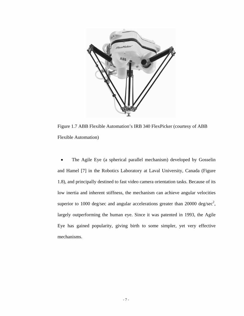
Figure 1.7 ABB Flexible Automation’s IRB 340 FlexPicker (courtesy of ABB

Flexible Automation)

• The Agile Eye (a spherical parallel mechanism) developed by Gosselin

and Hamel [7] in the Robotics Laboratory at Laval University, Canada (Figure

1.8), and principally destined to fast video camera orientation tasks. Because of its

low inertia and inherent stiffness, the mechanism can achieve angular velocities

superior to 1000 deg/sec and angular accelerations greater than 20000 deg/sec2,

largely outperforming the human eye. Since it was patented in 1993, the Agile

Eye has gained popularity, giving birth to some simpler, yet very effective

mechanisms.

- 7 -

Figure 1.8 The Agile Eye parallel robot (images courtesy of Robotics Laboratory at

University of Laval, Canada)

These are, of course, only some examples of widely known parallel manipulator

inventions.

1.2 Robotic Architectures

This section presents the three basic architectures for robot manipulators. These

architectures are characterized by the type of kinematic chains connecting the output

link of the manipulator to the base link. The three basic robot architectures are:

1) Serial architecture

2) Parallel architecture

3) Hybrid architecture

- 8 -

1.2.1 Serial Architecture

This is the classical anthropomorphic architecture for robot manipulators (Figure

1.9). In this architecture, the output link is connected to the base link by a single open

loop kinematic chain. The kinematic chain is composed of a group of rigid links

with pairs of adjacent links that are interconnected by an active kinematic pair

(controlled joint).

Figure 1.9 Serial Manipulator (taken by Jo Teichmann, Augsburg, Germany for

KUKA Robot GmbH, Year 2002)

Serial manipulators feature a large work volume and high dexterity, but suffer

from several inherent disadvantages. These disadvantages include low precision, poor

force exertion capability and low payload-to-weight ratio, motors that are not located at

the base, and a large number of moving parts leading to high inertia.

The low precision of these robots stems from cumulative joint errors and

deflections in the links. The low payload-to-weight ratio stems from the fact that every

- 9 -

actuator supports the weight of the successor links. The high inertia is due to the large

number of moving parts that are connected in series, thus forming long beams with high

inertia.

Another disadvantage of serial manipulators is the existence of multiple solutions

to the inverse kinematics problem. The inverse kinematics problem is defined as finding

the required values of the actuated joints that correspond to a desired position and

orientation of the output link. The solution of the inverse kinematic problem is a basic

control algorithm in robotics; therefore, the existence of multiple solutions to the inverse

kinematics problem complicates the control algorithm. The direct kinematics problem of

serial manipulators has simple and single-valued solution. However, this solution is not

required for control purposes. The direct kinematics problem is defined as calculating the

position and orientation of the output link for a given set of actuated joints values.

The low precision and payload-to-weigh ratio lead to expensive serial robots

utilizing extremely accurate gears and powerful motors. The high inertia disadvantage

prevents the use of serial robots from applications requiring high accelerations and agility,

such as flight simulation and very fast pick and place tasks.

1.2.2 Parallel Architecture

This non-anthropomorphic architecture for robot manipulators, although known

for a century, was developed mainly during the last three decades. This architecture is

composed of an output platform connected to a base link by several kinematic chains

(Figure 1.10). Motion of the output platform is achieved by simultaneous actuation of the

- 10 -

kinematic chains extremities. Similarly, the various kinematic chains support the load

carried by the output link; therefore, this architecture is referred to as parallel architecture.

In contrast to the open chain serial manipulator, the parallel architecture is composed of

closed kinematic chains only and every kinematic chain includes both active and passive

kinematic pairs.

Parallel manipulators exhibit several advantages and disadvantages. The

disadvantages of the parallel manipulators are limited work volume, low dexterity,

complicated direct kinematics solution, and singularities that occur both inside and on the

envelope of the work volume. However, the parallel architecture provides high rigidity

and high payload-to-weight ratio, high accuracy, low inertia of moving parts, high agility,

and simple solution for the inverse kinematics problem. The fact that the load is shared

by several kinematic chains results in high payload-to-weight ratio and rigidity. The high

accuracy stems from sharing, not accumulating, joint errors.

Based on the advantages and disadvantages of parallel robots, it can be concluded

that the best suitable implementations for such robots include those that require limited

workspace, high accuracy, high agility, and robots that are lightweight and compact.

These ideal implementations exploit both the disadvantages and advantages of the

parallel architecture.

- 11 -

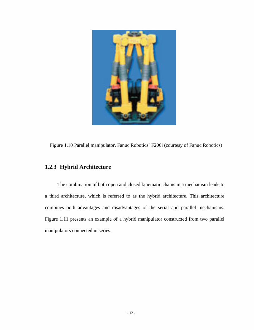
Figure 1.10 Parallel manipulator, Fanuc Robotics’ F200i (courtesy of Fanuc Robotics)

1.2.3 Hybrid Architecture

The combination of both open and closed kinematic chains in a mechanism leads to

a third architecture, which is referred to as the hybrid architecture. This architecture

combines both advantages and disadvantages of the serial and parallel mechanisms.

Figure 1.11 presents an example of a hybrid manipulator constructed from two parallel

manipulators connected in series.

- 12 -

Figure 1.11 Hybrid manipulator

1.3 Fully Parallel and Non-fully Parallel Manipulators

There are two major categories of parallel robots. They are the fully parallel robots,

and the non-fully parallel robots. The distinction between these categories is based on the

following definition. This definition is the same as the one presented in [8].

Definition: Fully parallel manipulator

A fully parallel manipulator is a parallel mechanism satisfying the following

conditions:

1) The number of elementary kinematic chains equals the relative mobility

(connectivity) between the base and the moving platform.

2) Every kinematic chain possesses only one actuated joint.

3) All the links in the kinematic chains are binary links; i.e., no segment of an

elementary kinematic chain can be linked to more than two bodies.

- 13 -

Based on the solution multiplicity of the inverse kinematics problem, this limiting

definition can be summarized as follows. A fully parallel manipulator has one and only

one solution to the inverse kinematics problem. Any parallel manipulator with multiple

solutions for the inverse kinematics problem is a non-fully parallel manipulator. Table 1.1

specifies the physical characteristics of serial and parallel manipulators.

Table 1.1 Comparison between Serial and Parallel manipulators

Property Serial Manipulator Parallel Manipulator

Type of kinematic

chains

Open kinematic chain Closed kinematic chain

Type of joints used Actuated joints Actuated and passive joints

The role of actuated joints Twist applicators Wrench applicators

Direct kinematics

problem

Simple and single-valued

solution

Complicated with up to

40 solutions

Inverse kinematics

problem

Complicated with

multiple solutions

Simple with multiple

solutions

Joint errors Cumulative Non-cumulative

Positional accuracy Poor Average

Payload-to weight ratio Low Very high

Singularity Loss of freedoms Gain and loss of freedoms

Singularity domain On the envelope of the

workspace

Both inside and on the

envelope of freedoms

Jocobian mapping Maps joint speeds to end

effector linear/angular

Maps the end effector

linear/angular velocity to

- 14 -

velocity actuated joint’s speeds

Work volume Large Small

Inertia of moving parts High Low

1.4 Summary of the Developed Robot

The first implementation of a parallel architecture by Gough and Whitehall [3]

presented six degrees of freedom tire test machine with base and moving platforms

interconnected by six extensible screw jacks (Figure 1.2).

In 1965, Stewart’s famous paper appeared in the proceedings of the (British)

IMechE. In that paper, Mr. Stewart describes a 6 –DOF motion platform for use as a

flight simulator (Figure 1.4) [4].

Later, all platforms based manipulators were called Stewart-Gough platform or

Stewart platforms.

Since 1980, there has been an increasing interest in the development of parallel

manipulators. Potential applications of parallel manipulators include mining machines by

Cleary and Arai [9], pointing devices by Gosselin and Angeles [10], and walking

machines by Waldron, Vohnout, Pery, and McGhee [11].

Hunt [12] suggested the use of parallel-actuated mechanisms like the flight

simulator of Stewart as robot manipulators and mentioned that such parallel manipulators

deserve detailed study in the context of robotic applications in view of their specific

advantages (e.g. better stiffness and precise positioning capability) over conventional

- 15 -

serial robots. This can be marked as the starting point of research on parallel

manipulators in general and the Stewart platform in particular in robotic applications.

The recent trend toward high-speed machining has motivated research and

development of new and novel types of machine tools called parallel kinematic machines

(PKMs). PKMs are based on the kinematic architecture of parallel manipulators. A

parallel manipulator typically consists of a moving platform that is connected to a fixed

base by several legs. The number of legs is usually at least equal to the number of degrees

of freedom of the moving platform, such that each leg is driven by no more than one

actuator and all actuators can be mounted on or near the fixed base. Note, that if the

number of legs is less than the number of degrees of freedom, then more than one

actuator will be needed in some legs. Examples of PKMs include the Variax Machining

Center developed by Giddings and Lewis [13], the Octahedral Hexapod by Ingersoll [14].

Most 6-DOF PKMs are based on the Stewart-Gough platform architecture.

However, six degrees of freedom are often not required for machine tools and other

applications due to a high cost. Therefore, parallel manipulators with less than six

degrees of freedom have attracted the researchers and some of them were used in the

structure designs of robotic manipulators. For example, the 3-RPS parallel platform was

adopted as a micromanipulator by Lee and Shah [16]; the 3-DOF spherical parallel

platform was used in the structure design of the “agile eye” by Gosselin and Hamel [7].

The direct drive DELTA manipulator with three translational degrees of freedom was

presented by Clavel [17] to meet the demand of high efficiency manipulation. Wang and

Gosselin [18,19] presented a 4-DOF and a 5-DOF parallel platforms and pointed out that

- 16 -

they can substitute the general 6-DOF parallel platform in the cases where less than six

degrees of freedom are sufficient for task manipulations.

Tsai [20] presented a 3-DOF parallel manipulator with more than three legs. The

additional legs permit a separation of the function of constraint from that of actuation at a

cost of increased mechanical complexity and chances of leg interference.

In a flexible automation approach to batch or job-shop production, the re-

configurability of the elements of a manufacturing system has proved to be important. A

key element of reconfigurable manufacturing systems is the reconfigurable machine tools

(RMT). Zhang and Bi [21] introduced the theoretical design of re-configurable machine

tools using modular design approach.

However, these manipulators have coupled motion between the position and

orientation of the end-effector. Therefore, the kinematics model is complex and the

manipulator is difficult to control.

Recent research on 3-DOF parallel manipulators has been leaning toward the

decoupling of the position and orientation of the end-effector. Kinematics decoupling for

a parallel manipulator is that one motion of the up-platform only corresponds to input of

one leg or one group of legs. In addition, the input cannot produce other motion. Tsai et

al. [22] designed a 3-DOF translational parallel manipulator that employs only revolute

joints and a spatial 3-UPU (Universal-Prismatic-Universal) parallel manipulator [23].

Kim and Tsai [24] discussed the optimal design about a 3-PRRR (Prismatic-Revolute-

Revolute-Revolute) manipulator. Zhao and Huang [25] studied the kinematics of an over-

constrained 3-RRC (Revolute-Revolute-Cylindrical) translational manipulator, and Kong

- 17 -

and Gosselin [26] studied the kinematics and singularity of a 3-CRR (Cylindrical-

Revolute-Revolute) translational parallel manipulator.

- 18 -

Chapter 2

Conceptual Design

2.1 Introduction

2.1.1 Classification of Kinematic Decoupling

The parallel manipulator whose motions are decoupled, i.e., some actuator

movements influence only some motion outputs, is called a decoupled manipulator.

The classification of kinematic decoupling can be sorted as following:

Let U, the kinematic output matrix of a parallel manipulator, to be

, ⎥⎦

⎤⎢⎣

⎡=

)()()()()()(

iii

iii zyxU

θγθβθαθθθ

1=i ~ M , (2.1)

where ),(),( ii yx θθ and )( iz θ denote the components of the origin coordinate of

the moving coordinate system attached to the moving platform with respect to the

reference coordinate system attached to the base platform, )(),( ii θβθα , and )( iθγ denote

the three Euler angles of the moving coordinate system, iθ denotes the generalized

variable of the actuator, and thi M denotes the mobility of the platform.

- 19 -

Take a 6-DOF parallel manipulator as an example; the kinematic relationship

between output and input variables can be classified as follows:

(1) If each of the independent output variable is a function of all input variables

iθ , ( 1=i ~ M ),

such as:

),...,,(),...,,(),...,,(

),...,,(),...,,(),...,,(

621

621

621

621

621

621

θθθγγθθθββθθθααθθθθθθθθθ

======

zzyyxx

(2.2)

the relationship between input and output variables is called coupling.

(2) If each of the independent output variable corresponds to only one input

variable,

such as:

)()()(

)()()(

6

5

4

3

2

1

θγγθββθααθθθ

======

zzyyxx

(2.3)

the relationship between input an output variables is called complete

decoupling .

(3) If the situation that is consistent with neither case (1) nor case (2) is called

partial decoupling. For instance:

- 20 -

)(),(

),,(),,,(

),,,(),,,,(

1

21

321

4321

54,321

654,321

θγγθθββ

θθθααθθθθ

θθθθθθθθθθθ

====

=

=

zzyyxx

(2.4)

Although the complete decoupling is a perfect model for the task specified,

designing mechanisms to truly realize this model is very difficult. Nevertheless, realizing

partial decoupling is also of significance especially when most of the known parallel

manipulators belong to the type of strong coupling. The high decoupling of a mechanism

makes kinematics and dynamics analyses easy, which can evidently simplify the control

and path planning of the manipulator. Therefore, from the point of view of improving

work performance of manipulators, it is necessary to investigate and synthesize

decoupled parallel manipulators.

2.1.2 Isotropy

We know that the Jacobian matrix of robotic manipulator is the matrix mapping (i)

the actuated joint velocity space, and the end-effector velocity space, and (ii) the static

load on the end-effector and the actuated joint forces or torques. Isotropic of a robotic

manipulator is related to the condition number of its Jacobian matrix, which can be

calculated as the ratio of the largest and the smallest singular values. A robotic

manipulator is fully isotropic if its Jacobian matrix is isotropic throughout the entire

workspace, i.e., the condition number of the Jacobian matrix is equal to one. Thus, the

- 21 -

condition number of the Jacobian matrix is an interesting performance index

characterizing the distortion of a unit ball under this liner mapping. The condition number

of the Jacobian matrix was first used by Salisbury and Craig [34] to design mechanical

fingers, and then developed by Angeles [35] as a kinematic performance index of robotic

mechanical systems. The isotropic design improves kinematic and dynamic performance

[36].

For parallel manipulators, the velocities of the moving platform are related to the

velocities of the actuated joint [ ]q& by general equation:

[A] [B] (2.5) =⎥⎦

⎤⎢⎣

⎡

P

O

ων

⎥⎦⎤

⎢⎣⎡ .q

where is the velocity of a point [ ] [ Tzyxv ννν= ] P belonging to the moving platform,

is the angular velocity of the moving platform, [A] is the direct Jacobian,

[B] is the inverse Jacobian, and O is the coordinate system in which the velocities of the

moving platform are expressed.

[ ] [ Tzyx ωωωω = ]

Equation (2.5) can also be written as a linear mapping between joint velocities and the

velocities of the moving platform.

[J] =⎥⎦

⎤⎢⎣

⎡

P

O

ων [ ]q& (2.6)

where [J]=[A]-1[B] (2.7)

is the global Jacobian including the direct and inverse Jacobians. For many architectures

of parallel manipulators, it is more convenient to study the conditioning of the Jacobian

that is related to the inverse transformation, i.e., [J]-1=[B]-1[A]

- 22 -

The isotropic conditions should apply to either Jacobian matrices A and B or only

to Jacobian matrix J or (J-1). If we have a matrix Q (which can be A, B, J, or J-1) whose

all entries have the same units, then we can define its condition number k(Q) as a ratio of

the largest singular value 1τ of Q and the smallest one 2τ . We note that k(Q) can attain

values from 1 to infinity. The condition number attains its minimum value of unity for

matrices with identical singular values.

We know that the singular values of Q are given by the square roots of the

eigenvalues of [Q]T[Q]. A matrix Q is isotropic if [Q]T[Q] is proportional to an identity

matrix I. So, the Jacobian matrices A, B, J, or J-1 are isotropic if [15]

[A]T[A] [I] (2.8) 21σ=

[B]T[B] [I] (2.9) 22σ=

[J]T[J] [I] (2.10) 23σ=

[J]-1[J]T [I] (2.11) 24σ=

where iσ ( 4,3,2,1=i ) is a scalar.

- 23 -

2.1.3 Screw Theory and Mobility Analysis

2.1.3.1 Screw and Reciprocal Screws

Screw theory was developed by Sir Robert Stawell Ball in 1876 [32], for

application in kinematics and statics of mechanisms (rigid body mechanics). It is a way to

express displacements, velocities, forces, and torques in three-dimensional space,

combining both rotational and translation parts. Recently, screw theory has regained

importance and has become an important tool in robot mechanics, mechanical design,

computational geometry, and multi-body dynamics.

In screw theory [33], a straight line in space can be expressed by two vectors, S

and S0. Their dual combination is called a line vector

$ = (S; S0) = (S ; r ×S) = ; o (2.12) l( m n p )q

where S is the unit vector along a straight line or a screw axis; l , , and n are the three

direction cosines of S; o ,

m

p , and q are the three elements of the cross product of r and S;

r is a position vector of any point on the line or screw axis. The (S, S0) is also called the

Plucker coordinates for the line vector and it consists of six components in total.

For a line vector, S ⋅ S0 = 0. When S ⋅ S0 =1, it is a unit line vector. When S ⋅ S0 ≠ 0, it is

a screw $ = (S; S0) = (S ; r × S + hS) and its pitch is finite. If the pitch of a screw is equal

to zero, the screw degenerates to a line vector. In other words, a unit screw with zero-

pitch is a line vector. The line vector can be used to express a revolute pair in )0( =h

- 24 -

kinematics, or a unit force in static along the line in space. If the pitch of a screw goes to

infinity, , the screw is defined as ∞=h

$=(0; S)=(0 0 0; (2.13) l m )n

and called a couple in screw theory, which means a unit screw with infinity-pitch ( ∞=h )

is a couple. The couple can be used to express a prismatic pair in kinematics or a couple

in statics. S is its direction cosine.

Both the revolute joint and prismatic joint is of the single-DOF kinematic pair.

The multi-DOF kinematic pairs, such as cylinder joint, universal joint, or spherical joint

can also be represented by a group of screws because of its kinematic equivalency to a

combination of revolute and prismatic pairs.

The reciprocal product of two screws, say $ = (S ; S0) and, $r = (Sr ; S r0 ) is defined

as [33] [61]

$ ο $r = S ⋅ S + Sr ⋅ S0 (2.14) r0

Where, the symbol “ ” denotes the reciprocal product of two screws. The reciprocal

product of two screws represents the work produced by a wrench acting on a rigid body

undergoing an infinitesimal twist.

ο

Two screws are said to be reciprocal if their reciprocal product is zero

$ ο $r = (2.15) 0=+++++ rrrrrr qnpmolnqmplo

Equation (2.15) shows that the wrench $r acting on a rigid body undergoing an

infinitesimal twist $ yields no work. Then, the wrench $r denotes a constraint force when

its pitch is zero, or a constraint couple when its pitch is infinite. The former restricts a

translational freedom of the rigid body along the direction of the force, and the latter

restricts a rotational freedom around the axis of the couple.

- 25 -

The reciprocal equation of two screws is also expressed as follows [61]:

0sincos)( 12121221 =−+ λλ rhh (2.16)

Where, is the normal distance of the two screws and 12r 12λ is the twist angle between the

two screws. Clearly, when two line vectors intersect or are parallel to each other, the two

screws are reciprocal.

According to equations (2.15) and (2.16), some useful reciprocal conditions for

two screws can be concluded simply as in Table 2.1.

Table 2.1 Reciprocal conditions for two screws

Number Reciprocal conditions

1 The sufficient and necessary condition for reciprocity of two line

vectors is coplanar.

2 Any two couples are consequentially reciprocal

3 A line vector and a couple are reciprocal only when they are

perpendicular

4 Any two screws are consequentially reciprocal when they are

perpendicular and intersecting

5 Both the line vector and couple are self-reciprocal, respectively

For mobility analysis, from equation (2.15) we can get the reciprocal screws.

Sometimes, using Table 2.1 is more convenient than that of equation (2.15). The

correctness of these two methods is often proven by each other.

Furthermore, reciprocity of screws is origin independent, which is easy to prove from

equation (2.16). There also exist similar results for the linear dependency of screws.

- 26 -

2.1.3.2 Screw Systems and Reciprocal Screw Systems

A screw system of order N )60( ≤≤ N comprises all the screws that are linearly

dependent on N given linearly independent screws. A screw system of order N is also

called an N -system. Any set of N linearly independent screws within an N -system

forms a basis of the N -system. Usually, the basis of an N -system can be chosen in

different ways. Given an N -system, there is a unique reciprocal screw system of

order , which comprises all the screws reciprocal to the original screw system. )6( N−

2.1.3.2 Twist Systems and Wrench Systems

A screw $ multiplied by a scalar ρ , i.e., ρ $, is called a twist if it represents an

instantaneous motion of a rigid body, and a wrench if it represents a system of forces and

couples acting on a rigid body.

The twist system of a kinematic chain, in the form of a kinematic joint, serial

kinematic chain or parallel kinematic chain, is an -system where and

denotes the DOF of the kinematic chain. The wrench system of a kinematic chain is a

-system. The twist system of a kinematic chain is the reciprocal screw system of

its wrench system, and vice versa.

f Ff ≤ F

)6( f−

The twist systems and wrench systems of revolute (R) joint, prismatic (P) joint,

universal (U) joint and Cylinder (C) joint are presented below.

(i) R (Revolute) joint

- 27 -

The twist system of an R joint is a 1-system. The wrench system is a 5-system

(ii) P (Prismatic) joint

The twist system of a P joint is a 1-system. The wrench system is a 5-system

(iii) U (universal) joint

The twist system of a U joint is a 2-system. The wrench system is a 4-system

(iv) C (Cylinder) joint

The twist system of a C joint is a 2-system. The wrench system is a 4-system

- 28 -

2.1.3.3 Mobility Analysis Based on Screw Theory

The general Chebyshev-Grubler- Kutzbach formula is:

∑=

+−−=g

iifgdM

1

)1(η (2.17)

where:

M : Mobility or the degree of freedom of the system.

d : The order of the system ( = 3 for planar mechanism, and = 6 for spatial d d

mechanism).

η : The number of the links including the frames.

g : The number of joints.

if : The number of degrees of freedom for the ith joint.

One drawback of the Chebyshev-Grubler-Kutzbach formula is that it can only

derive the number of DOF of some mechanisms, but cannot obtain the properties of the

DOF, i.e., whether they are translational or rotational DOF.

For a lower-mobility parallel mechanism, each leg exerts some structural

constraints on the moving platform. The combined effect of all the leg structural

constraints determines the mobility of the mechanism. We use the leg constraint system

to describe the structural constraints of a single leg, which is defined as a screw system

formed by all screws reciprocal to the unit twist associated with all kinematic pairs in a

leg. We use the mechanism constraint system to describe the combined effect of all leg

constraints.

- 29 -

Based on linear dependency of the leg structural constraints under different geometrical

conditions, we can obtain the mechanism constraint system as well as the constrained

DOF of the moving platform.

Because twists and wrenches are instantaneous, it is necessary to identify whether

the mechanism is instantaneous. This can be obtained by verifying the mechanism

constraint system after any arbitrary finite displacement. If the mechanism constraint

system remains unchanged, the mechanism is non-instantaneous. Such verification can

be done by simple analysis and inspection of structural or geometrical conditions

among the kinematic pairs in each leg and the mechanism. It is not necessary to know

the analytical expressions of the mechanism constraints including the analytical

expressions of the finite displacements in all joints of each leg.

Let $ represent the unit twist associated with the kinematic pair in the leg;

$ rij is used to represent the unit wrench exerted by the leg; $ is used to represent

the unit twist in the mechanism twist system; $ is used to represent the unit

wrench in the mechanism constraint system.

ijthj thi

thj thi mj

thj rmj

thj

Assume that a M-DOF (M< 6) parallel mechanism has ξ legs and each leg exerts

ζ structural constraints on the moving platform. The ζξ ⋅ constraints form the

mechanism constraint system, which must be a 6- M system in the general non-singular

configuration.

Because most of the lower-mobility parallel mechanisms are over-constrained, it

is necessary to take the common constraints of mechanism and the passive constraints

into consideration in mobility analysis. Thus, we rewrite the general Chebyshev-Grubler-

Kutzbach formula as

- 30 -

(2.18) νη ++−−= ∑=

g

iifgdM

1

)1(

where ν is the number of passive constraints.

The order of a mechanism is given by

ε−= 6d (2.19)

where ε is the number of the common constraints. The common constraint is defined

as a screw reciprocal to all unit twists associated with kinematic pairs in a lower-

mobility parallel mechanism. A common constraint exists if and only if each leg

provides one constraint and all the ξ constraints are coaxial; namely, they form an l-

system.

Considering the remaining leg constraints except those leg constraints, which

form the common constraints. If they are linearly dependent, there exist passive

constraints.

Assume that the remaining leg constraints form a l - system, the number of

passive constraints is given by

l−⋅−⋅= ξεζξν (2.20)

It should be noted that the ζξ ⋅ leg constraints must equal the sum of the 6-M

mechanism constraints, the leg constraints which form the common constraints, and

the passive constraints. Considering that each common constraint constrains one DOF

of the moving platform, we have

vM +⋅+−−=⋅ ξεεζξ )6( (2.21)

Thus, a general mobility criterion for the lower-mobility parallel mechanisms can

also be obtained [62]

- 31 -

νξεζξ +−+⋅−= )1(6M (2.22)

Equations (2.20) and (2.22) are actually established based on constraint analysis.

They’re applicable to both symmetrical and asymmetrical lower-mobility parallel

mechanisms.

The mobility analysis of lower-mobility parallel manipulators can be performed

following the steps below:

Step 1 In the initial configuration, first write out the leg twist system, and then

obtain the leg constraint system. Hence, ζ is available in this step.

Step 2 According to the linear dependency of all leg constraints under different

geometrical conditions obtain the mechanism constraint system as well as the

constrained freedoms. In this step, ε and ν are also available.

Step 3 Check whether the mechanism is instantaneous. Simply judging if the

mechanism constraint system remains unchanged after any non-singular feasible finite

displacement can do this.

Step 4 Use equations (2.19) and (2.22) to verify the mobility.

- 32 -

2.1.4 Over-Constrained Parallel Manipulator

Usual parallel manipulators, like the Stewart platform, suffer from the problems

of difficult forward kinematics, coupled motion, and small workspace, so as to make

motion planning and control difficult in applications. The parallel manipulator with lower

mobility (DOF<6) can relatively reduce the complexity. However, most of the parallel

manipulators with lower mobility are over-constrained when assembly errors are

considered [29].

Over-constrained parallel kinematic manipulators are those with limbs that

provide similar constraint(s) [12]. That is, the other limb also provides the motion

constraint provided by one limb. These over-constrained mechanisms do move despite

the fact that Grubler / Kutzbach criterion in its original form [6,12,30] concludes that they

should not, and they (over-constrained mechanisms) are mobile only when certain

geometrical conditions are satisfied. Although they have some advantages, such as using

fewer joints and links, resulting in a simple mechanism, the main price of these over-

constrained mechanisms is the need for strict manufacturing tolerance and the excessive

loads on some links and/or joints. Therefore, these parallel manipulators cannot be

assembled without joint clearance, which imposes negative impacts on the accuracy of

the end-effector.

However, using inactive joints can reduce the number of over-constraints of a

parallel manipulator [31].

- 33 -

2.2 Geometrical Design

In this section, we focus on the conceptual design of a 3-DOF non-over

constrained translational PKM with decoupled motions. It can be used for parts assembly

and light machining tasks that require large workspace, high dexterity, high loading

capacity, and considerable stiffness. Kinematically, a 3-DOF non-over constrained PKM

also implies that each leg should have an inactive joint.

To simplify the design and development efforts, we have the following additional

considerations:

• The PKM is composed of a base and a moving platform connected by three legs

• Symmetric design - each leg is identical to the others. Hence, each leg should

have the same number of actuated joints.

• Type of joints – four types of commonly used joints are considered:

(i) 1-DOF revolute (R) joint

(ii) 1-DOF prismatic (P) joint

(iii) 2-DOF universal (U) joint

(iv) 2-DOF cylinder (C) joint

Among them, the revolute and universal joints are only meant for passive (i.e. not

actuated) joint, the prismatic or the prismatic in the cylinder joints are only meant

for actuated joints.

• Actuated joints are placed close to the base so as to reduce the moment of inertia

and increase the loading capacity and motion acceleration.

- 34 -

• At most one (actuated) prismatic or cylinder joint can be employed in each of the

legs due to its heavy and bulky mechanical structure.

• The number of redundant DOF of a leg is not greater than one (1).

• The number of inactive joint of all legs is not greater than one (1).

• Each leg is composed of a group of at least three revolute joints with parallel axes

and at most one revolute joint whose axis is not parallel to the axes of the revolute

joints in the group of revolute joints with parallel axes, while the axis of the

actuated joint (prismatic or cylinder) is not perpendicular to the axes of the

revolute joints in the group of revolute joints with parallel axes.

• The axes of all the revolute joints in the group of revolute joints with parallel axes

are not parallel to a plane.

• The axes of all three actuated joints should be arranged perpendicular to each

other to satisfy the parallel manipulator featuring decoupled motion.

With these design considerations, a novel 3-CRU non-over constrained

translational PKM with decoupled motions has been proposed. The 3-CRU (Figure 2.1) is

composed of a base and a moving platform connected by three CRU legs.

The axes of the C and R joints, as well as the axe of the U joint, are arranged such

that their joint axes are parallel to a common plane. As a result, the axe of outer R joint

(the one connects to the moving platform) of the U joint is perpendicular to the axe of the

U joint as well as all the axes of the C and R joints within a given leg. All above

guarantee that instantaneous rotation of the moving platform about a direction that is

perpendicular to the common plane of all the axes of the C, R, and inner R of the U joint

is impossible. Since each C joint can be considered as a combination of one R joint and

- 35 -

one P joint with parallel axes, each U joint consists of two intersecting R joints; each leg

is kinematically equivalent to a PRRRR chain.

Through preliminary analysis, a 3-DOF PKM with such three CRU legs possesses

the following advantages:

Simple kinematics and easy for analysis, design, trajectory planning, and motion

control

Large and well shaped workspace

High stiffness

High loading capacity

“ ” is the direction of the liner motor

Figure 2.1 CAD Model of 3-CRU

- 36 -

- 37 -

A1

A2

z y

o

x

Figure 2.2 Schematic Model of 3-CRU

R2 R1 B22

R3

A3

B21

B11 w

B31

B32

B12 u

v

2.3 Mobility Analysis of the Manipulator

For the 3-CRU manipulator, we have ,1=ζ and mechanism obviously contains

no common constraints and redundant constraints, then we have ,0=ε and 0=υ .

Using equation (2.18), we have:

30)212(*3)198(*6 =++++−−=M (2.23)

Using equation (2.22), we have

301*36 =+−=M (2.24)

For a parallel manipulator with less than six degrees of freedom, the motion of

each leg that can be treated as a twist system is guaranteed under some exerted structural

constraints, which are termed as a wrench system. The wrench system is a reciprocal

screw system of the twist system for the same leg, and a wrench is said to be reciprocal to

a twist if the wrench produces no work along the twist. The mobility of the manipulator is

then determined by the combined effect of wrench systems of all legs.

For the 3-CRU manipulator, the wrench system of a leg is a 1-system, which

exerts one constraint couple to the moving platform with its axis perpendicular to the axis

of C joint within the same leg. The wrench system of the moving platform, that is a linear

combination of wrench systems of all the three legs, is a 3-system, because the three

wrench 1-systems consist of three couples, which are linearly dependent and form a

screw 3-system. Since the arrangement of all the joints shows on Figure 2.1, the wrench

systems restrict three rotations of the moving platform with respect to the fixed base at

any instant, thus leading to a translational parallel manipulator.

- 38 -

2.4 Inactive Joint

A general leg for a translational parallel manipulator with a liner actuator is

composed of ( 1−ψ ) R joints and one P or C joints. For the purposes of simplification,

the P joint (or the P joint of the C joint) is labeled with 1, while the R joints (including

the R joint of C joint) are labeled with 2, 3…, and ψ is the sequence from the base to the

moving platform.

The infinitesimal change of orientation of the moving platform is a serial

kinematic chain undergoing infinitesimal joint motion is [31]

si) (2.25) ∑=

Δ=Δn

iiR

2( θ

where RΔ and iθΔ denote the infinitesimal change of orientation of the moving platform

and the infinitesimal joint motion of joint i respectively; si denotes the unit vector along

the axis of joint i before the infinitesimal motion.

For a translational parallel manipulator, there exists

(2.26) 0=ΔR

Substitution of equation (2.25) into equation (2.26), yields

si ) = 0 (2.27) ∑=

Δn

ii

2

( θ

For the 3-CRU parallel manipulator, the only R joint whose axis is not parallel to

the axes of the other R joints is labeled with 5. It exits

s5 s4 = s3 = s2 (2.28) ≠

- 39 -

Substitution of equation (2.28) into equation (2.27), yields

s5 si =0 (2.29) ∑=

Δ+Δ4

25

iiθθ

To satisfy equation (2.29), we have

05 =Δθ (2.30)

and

(2.31) ∑=

=Δ4

2

0i

iθ

Equation (2.30) proves that the outer R joint of the U joint of each leg is inactive.

Equation (2.31) shows that the R joints with parallel axes within the same leg constitute a

dependent joint group.

An inactive joint is a joint in a leg whose joint variable is constant during the motion of

the manipulator. Although when an inactive joint is removed, the relative motion within

the leg will not be changed, by using inactive joints, the number of over-constraints of the

translational parallel manipulator in this thesis can be reduced.

- 40 -

Chapter 3

Kinematic Modeling of the 3-CRU Parallel

Manipulator

3.1 Introduction

The kinematics of a robot deal with finding the analytical relations between its

input variables (the values of the actuated joints) and output variables (the position and

orientation of the moving platform); the equations that connect the input and the output

variables of a mechanism are called the kinematic equations of the mechanism. The

equations that connect input and output velocities in a mechanism are called the

instantaneous kinematic variables of the robot, i.e., the position and orientation of the

moving platform, for a given set of input variables, namely, the actuated joints’ variables.

The inverse kinematics problem deals with finding the required input variables (actuated

joints’ values) that correspond to a given set of output variables (position and orientation

of the moving platform).

- 41 -

The inverse kinematics problem of the Stewart-Gough manipulator [6] is trivial

with single solution, but when the number of kinematic chains is reduced, the number of

solutions of the inverse kinematics problem increases and the problem becomes more

challenging. The direct kinematics problem of parallel manipulators is by far more

challenging than the inverse kinematics problem since it requires solving a set of

polynomial equations in the output variables. While the inverse kinematics problem for a

general Stewart-Gough manipulator has only one solution, the direct kinematic problem

has up to forty (40) real solutions [30]. Dietmaier [65] systematically changed the

geometric properties of a general Stewart-Gough manipulator and for the first time, gave

an example of a manipulator with forty (40) real solutions to the direct kinematics

problem.

3.2 Inverse Kinematics

The purpose of the inverse kinematics issue is to solve the actuated variables

from a given position of the mobile platform.

To facilitate the analysis, referring to Figure 3.1, we define a fixed reference

frame -O xyz at the centered point O on the base and a moving reference frame -uvw

at the centered point P on the moving platform, with the and w axes perpendicular to

the platform, and the

P

z

x and axes parallel to the u and axes, respectively. The

direction of the ith fixed C joint is denoted by unit vector ci . A reference point is

defined on the axis of the ith fixed C joint, and the sliding distance is defined by ;

y v

iM

id

- 42 -

point defined as the interaction of the axes of the U joint. Furthermore, the position

vector of point in the fixed frame is denoted by mi = [ ]T, while the

position vector of point is noted by b i = [ ]T in the moving frame and bi in

the fixed frame. The ui is defined as a vector connecting Ai to Bi, and is orthogonal to the

unit vector ri = [ ]T .

iB

iM ziyixi mmm ,,

iB pziyixi bbb ,,

ziyixi rrr ,,

Generally, the position and orientation of the moving platform with respect to the

fixed base frame can be described by a position vector p= [ ]T and a 3 x 3 matrix

R .

zyx ppp

op

ci ei ri w Ai vv ui Bi l1i ri l2i di Ri p Mi mi O

Figure 3.1 Kinematic modeling of a leg

x

y z

v up bi

- 43 -

Since the moving platform of a 3-CRU possesses only translational motion, o R .

becomes an identity matrix. Then, we have

p

bi = b i (3.1) p

Referring to Figure 3, a vector-loop equation can be written for each leg as follows:

ui = p + bi - mi – dici (3.2)

Substituting equation (3.1) into equation (3.2), we have:

ui = p + b i - mi - dici (3.3) p

As vectors ui and ri are orthogonal, we yield:

u ri = 0 (3.4) Ti

Substituting equation (3.3) into equation (3.4), we get: (p + p b i - mi -dici)Tri = 0 (3.5)

For geometric parameters of this parallel manipulator, we have:

c1 = r1 = [1,0,0]T (3.6)

c2 = r2 = [0,1,0]T (3.7)

c3 = r3 = [0,0,1]T (3.8)

e1 = [0,0,1]T (3.9)

e2 = [0,0,1]T (3.10)

e3 = [1,0,0]T (3.11)

Substituting equations (3.6) to (3.11) into equation (3.5), we yield the solution of the

inverse displacement analysis for the 3-CRU parallel manipulator as:

d1 = px + bx1 – mx1 (3.12)

- 44 -

d2 = py + by2 – my2 (3.13)

d3 = pz + bz3 – mz3 (3.14)

From equations (3.12) to (3.14), we can easily observe that the motions of the 3-

CRU parallel manipulator are decoupled. The actuator in leg 1 controls the translation

along the X direction; the actuator in leg 2 controls the translation along the Y direction

while the actuator in leg 3 controls the translation along Z direction.

The distance between the center of the moving plate and base is mi = l2i + b

3.3 Forward Kinematics

The forward kinematics is to obtain the end-effector position, [ ] ,

when the input sliding distance di is given.

zyx ppp ,, T

By solving Equations (3.12) to (3.14) for variables x, y, and z, the forward

kinematics can be performed. Thus, we yield:

111 xxx mbdp +−= (3.15)

222 yyy mbdp +−= (3.16)

333 zzz mbdp +−= (3.17)

3.4 Velocity Analysis

Equations (3.15) to (3.17) can be rewritten as:

- 45 -

(3.18) ⎥⎥⎥

⎦

⎤

⎢⎢⎢

⎣

⎡

−+−+−+

=⎥⎥⎥

⎦

⎤

⎢⎢⎢

⎣

⎡

33

22

11

3

2

1

zzz

yyy

xxx

mbpmbpmbp

ddd

Taking the derivative of equation (3.18) with respect to time yields:

J (3.19) =

⎥⎥⎥⎥

⎦

⎤

⎢⎢⎢⎢

⎣

⎡

3

.2

.1

.

ddd

⎥⎥⎥⎥⎥

⎦

⎤

⎢⎢⎢⎢⎢

⎣

⎡

z

y

x

p

p

p

.

.

.

where J is the 3 x 3 identity matrix. Since J is an identity matrix, the manipulator is

isotropic everywhere within its workspace.

Therefore, the velocity equations of the 3-CRU parallel manipulator can be written as:

xpd.

1 =&

ypd.

2 =& (3.20)

zpd.

3 =&

3.5 Singularity Analysis

3.5.1 Constraint Singularity

The constraint singularity [63] occurs when the moving platform of a translational

parallel manipulator can rotate instantaneously. The constraint singularity occurs for a

- 46 -

translational parallel manipulator if and only if its wrench system (a 3-system of −∞

pitch) degenerates into a 2-system or a 1-system.

For the 3-CRU translational parallel manipulator, as ri≠ ei, the CRU leg exerts

one constraint on the moving platform, which prevents it from rotating about any axis

parallel to ri × ei. Therefore, the wrench system of the leg is invariant. The order of the

wrench system of the 3-CRU is thus a constant. That is to say, the 3-CRU translational

parallel manipulator is free from constraint singularity.

3.5.2 Kinematic Singularities

When type II kinematic singularity occurs for a parallel manipulator, the moving

platform can undergo infinitesimal or finite motion when the inputs are specified. It will

be proved below that, there is no type II singularity for the 3-CRU translational parallel

manipulator.

From Section 3.5.1, it is known that no rotation singularity exists for the 3-CRU

translational parallel manipulator. Thus, equation (3.19) is always satisfied. Uncertainty

singularities for the 3-CRU translational parallel manipulator occur if and only if J is

singular.

From Section 3.4, it is known that the Jacobian matrix, J, is an identity matrix.

Thus, no type II singularity exists for the 3-CRU translational parallel manipulator.

- 47 -

3.6 Stiffness Analysis

3.6.1 Introduction

Compare with serial manipulators, parallel manipulators offer an improved

stiffness and better accuracy. This feature makes them attractive for innovative machine

tool structures for high speed machining [37, 38, 39].

The stiffness properties of a manipulator can be defined through a 6 x 6 matrix

that is called stiffness matrix K.

Several methods exist for the computation of the stiffness matrix: the Finite

Element Analysis (FEA) [40], the matrix structural analysis (SMA) [41], and the virtual

joint method (VJM) which is also called the lumped modeling [42, 43].

The FEA is proved to be the most accurate and reliable; however, this method has

the disadvantage that it requires an extensive computation time [44]. The SMA also

incorporates the main ideas of the FEA, but operates with rather large elements, 3D

flexible beams describing the manipulator structure. This leads obviously to the reduction

of the computational expenses, but does not provide clear physical relations required for

the parametric stiffness analysis. Finally, the VJM method is based on the expansion of

the traditional rigid model by adding the virtual joints, which describe the elastic

deformations of the links.

- 48 -

3.6.2 General Stiffness Model for Parallel Manipulator

As introduced in Section 3.6.1, there are three methods to build mechanism

stiffness models. Among them, the method that relies on the calculation of the parallel

mechanism’s Jacobian matrix is adopted in this thesis [42, 43].

The stiffness of a parallel mechanism is dependent on the joint’s stiffness, the legs

structure and material, the platform and base stiffness, the geometry of the structure, the

topology of the structure and the end-effector position and orientation.

The stiffness of a parallel mechanism at a given point of its workspace can be

characterized by its stiffness matrix. This matrix relates the forces and torques applied at

the gripper link in Cartesian space to the corresponding linear and angular Cartesian

displacement. It can be obtained using kinematic and static equations.

Note, that link stiffness is not considered in conventional joint stiffness analysis

approach. That means links of the mechanism are assumed strictly rigid.

The joint displacement, qΔ , is related to the end-effector displacement in

Cartesian space rΔ , by the conventional Jacobian matrix J,

=Δq J rΔ (3.22)

Under the principle of virtual work, the end-effector force F in terms of the

actuated joint torques τ is given as the following:

=F JTτ (3.23)

Then τ can be related to qΔ by a diagonal actuated joint stiffness matrix

K whose elements are the stiffness of each actuator, as follow: ],,.......[ 1 nJ kkdiag= ik

=τ K J qΔ (3.24)

- 49 -

Substituting equation (3.22) into equation (3.24) and the resulting equation into equation

(3.23), then we have:

=F JTK JJ rΔ (3.25)

Therefore, the stiffness matrix of a parallel manipulator is given by:

Kr = JT K J (3.26) J

Particularly, in the case for which all the actuators have the same stiffness, i.e.,

, then equation (3.26) will be simplified to: nkkk === .....21

K = k JTJ (3.27)

which is the equation given in [42]

3.6.3 Stiffness Mapping

As introduced in Section 3.4, J is a 3 x 3 identity matrix, so we have JTJ = 1, the

stiffness matrix of this 3-CRU manipulator is

K = k (3.28)

The above model is now used to obtain the stiffness maps for this 3-DOF

decoupled parallel manipulator. A program has been written with the software Matlab.

Given the value in Tables 3.1 to 3.3, the stiffness mesh graphs in X, Y, Z are shown in

Figures 3.2 to 3.4.

From the stiffness mesh graphs in X (Figure 3.2), Y (Figure 3.3), and Z (Figure

3.4), one can conclude that the stiffness in X, Y, and Z will not change while the position

and orientation are changing. That means the stiffness of the actuators is the main factor

- 50 -

to determine the stiffness in the situations. The results also indicate that the stiffness is a

constant within its workspace; this will improve the kinematic accuracy.

As a result, the desired stiffness on X, Y, and Z directions can be achieved by

adjusting the stiffness of the actuators. Moreover, when using this 3-DOF parallel

manipulator for parts assembly or as a machine tool, one can judge if the parallel

manipulator is stronger enough to perform the tasks by considering the workloads in X, Y,

and Z directions.

Table 3.1 Stiffness in X vs. Stiffness to actuators

K N/m k N/m

500 500

Table 3.2 Stiffness in Y vs. Stiffness of actuators

K N/m k N/m

500 500

Table 3.3 Stiffness in Z vs. Stiffness of actuators

K N/m k N/m

500 500

- 51 -

-100-50

050

100

200

250

300499

499.5

500

500.5

501

stiff

ness

Stiffness in X with k=500 N/m

xy

Figure 3.2 Stiffness mesh graphs in X with k =500 N/m

- 52 -

-100-50

050

100

200

250

300499

499.5

500

500.5

501

stiff

ness

Stiffness in Y with k=500 N/m

xy

Figure 3.3 Stiffness mesh graphs in Y with k = 500 N/m

- 53 -

-100-50

050

100

200

250

300499

499.5

500

500.5

501

stiff

ness

Stiffness in Z with k=500 N/m

xy

Figure 3.4 Stiffness Mesh Graphs in Z When k = 500 N/m

- 54 -

Chapter 4

Workspace Analysis and Prototype Design

4.1 Definition of the Workspace

The workspace of the Parallel robot can be defined as a reachable region of the origin

of a coordinate system attached to the center of the moving plate. Since its major

drawback is a limited workspace, it is of primary importance to develop algorithms by

which the workspace can be determined and the effect of different designs on the

workspace can be evaluated.

There are several types of workspace [6]:

• Constant orientation workspace or translation workspace

• Orientation workspace

• Maximal workspace or reachable workspace

• Inclusive orientation workspace

• Total orientation workspace

• Dextrous workspace

• Reduced total orientation workspace

- 55 -

Various approaches may be used to calculate the workspace of a parallel

manipulator, such as geometrical approach, discretisation method, and numerical

methods [6].

The most common one is the geometrical approach. The purpose of this approach

is to determine the boundary of the robot workspace geometrically.

4.2 Workspace Analysis of the 3-CRU Parallel Manipulator

From equations (3.15) to (3.17), it appears clearly that the Cartesian workspace

consists of a parallelepiped. A regular workspace (parallelepiped) is very attractive in

practice.

Since we use linear actuators for the 3-CRU parallel manipulator, the workspace

is limited by the stroke lengths di. However, it is preferable to make the links of length l1i

and l2i sufficiently long to ensure that additional constraints are not imposed on the

mechanism, so that the ranges of motion of all linear actuators can be fully utilized. To

implement this, we applied the constraint that the workspace volume is always equal to

the product of the stroke lengths of the linear actuators.

Finally, we obtain the workspace of the parallel manipulator shown in Figure 4.1.

- 56 -

-100

1020

3040

-100

1020

3040

-10

0

10

20

30

40

x(cm)y(cm)

z(cm

)

Figure 4.1 Workspace

4.3 Prototype Design

Based on the 3-CRU architecture described in Chapter two, we focus on the

prototype design of the manipulator in this section.

The key issues in the detailed design of the 3-CRU translational parallel

manipulator are described as follows:

1. Adopt linear actuation layout; a linear actuator drives the C joint in each leg (see

Figure 2.1 for detail), whereas all the other joints are passive. One of the advantages is to

- 57 -

have all actuators installed on the fixed base. The C joints will be driven using toothed

belts connected to DC servomotors.

2. The selection of the assembly modes of each leg

In selecting the assembly modes of each leg, the location of the work piece to be

placed should be taken into consideration.

For the 3-CRU translational parallel manipulator, the work piece is placed under

the moving platform.

3. The determination of the link lengths of and il1 il2

In determining the link lengths and , the issue of avoiding link interferences

should be taken into consideration.

il1 il2

To address this issue, and are adjusted to avoid interference among links in

the three legs and the moving platform by simulating the motion of the parallel

manipulator using a CAD software.

il1 il2

Consider the requirements of feasibility concerning dimensional limits for

manufacturing parts, encoders available in the market, and the need for a continuous

working space with no interference of moving parts, the following choices for the

geometric parameters of the 3-CRU manipulator (see Figure 3.1 for d, l, b, and m):

Stroke length: mm 220321 === ddd

Length of leg: mm 32521 == ii ll

Dimension of the moving plate: 30=b mm

The distance between the center of the moving plate and base: 3552 =+= blm i mm

- 58 -

Chapter 5

Design Optimization

5.1 Introduction

Optimization is to find the best solution for a problem under given circumstance.

Mathematical optimization means that the problem at hand is formalized in a stringent

mathematical way and the best solution under the given circumstances is found by using

mathematical algorithms. When it comes to design optimization, Papalambros et al. give

the following definition in [45]:

Informally, but rigorously, we can say that design optimization involves:

1. The selection of a set of variables to describe the design alternatives.

2. The selection of an objective (criterion), expressed in terms of the design

variables, which we seek to minimize or maximize.

3. The determination of a set of constraints, expressed in terms of the design

variables, which must be satisfied by an acceptable design.

4. The determination of a set of values for the design variables, which minimize

(or maximize) the objective, while satisfying all the constraints.

- 59 -

There are many different optimization algorithms used in engineering design. The

algorithms can be divided into gradient-based and non gradient-based methods. The

gradient-based methods have been thoroughly studied and a considerable body of

literature is available on the subject [46-48]. The gradient- based methods are suitable for

problems with continuous variables and differentiable functions since they operate with

gradients of the problem functions.

Direct search methods are one example of algorithms, which do not calculate

derivatives. Examples of direct search methods include the Nelder-Mead simplex method

[49], Box’s Complex method [50], the Hooke and Jeeves pattern search [51], and the

Dennis and Torczon parallel direct search algorithm (PDS) [52]. A thorough review of

direct search methods can be found in [53]. Other non-gradient methods are stochastic

methods such as Genetic algorithms (GA) [54] are comprehensively studied in [55].

Simulated annealing was developed by Kirkpatrick [56] in the early 1980s. More recent

methods include Tabu search, developed by Glover [57], response surface

approximations [58], Taguchi methods [59], and Particle Swarm (PS) [60].

5.2 Genetic Algorithms

Genetic algorithm (GA) is a search algorithm based on the hypothesis of natural

selection and genetics. In the methods, each optimization variable is encoded by a gene

using an appropriate representation. The corresponding genes for all parameters form a

chromosome (or point) capable of describing an individual design solution. A finite

- 60 -

length string, such as a binary string of zeros and ones, is usually used to represent each

chromosome.

Today real value chromosomes are common, whereas original GAs used binary

representations of the optimization variables. A set of alternative points (called

population) at an iteration (called generation) is used to generate a new set of points. In

this process, combinations of the most desirable characteristics of the current members

(individuals) of the population are used to generate new populations better than the

current ones. When comparing different points the term fitness is used. Fitness is defined

using the objective function or the penalty function for constrained problems. The fitness

value is calculated for each member of the population, such that the fittest individuals are

the ones with the highest likelihood of survival.

The Genetic Algorithm starts with a set of randomly generated individuals (points). Three

operators are then needed to implement the algorithm: (i) selection; (ii) crossover; and (iii)

mutation. Selection is an operator where an old string (point) is copied into the new

population according to its fitness. Individuals with higher fitness are more likely to

produce offspring. The crossover operator corresponds to allowing the selected

individuals to exchange characteristics among themselves. Crossover entails selection of

starting and ending positions on a pair of mating strings at random and simply

exchanging the strings of zeros and ones between these positions. Mutation corresponds

to selection of a few individuals of the population, determining a location on the string at

random and switching the 0 to 1 or vice versa. The foregoing three steps are repeated for

successive generations of the population until no further improvement in the fitness is

- 61 -

possible, or the number of generation reaches a specified limit. The individual in this last

generation with the best fitness value is taken as the optimum.

5.3 The Optimum Design for the 3-CRU Manipulator with

Prescribed Workspace

Parallel mechanisms create great interest because they can be used for many

applications in industrial such as machine tools or light assembly.

Obtaining high performance requires the choice of suitable mechanism

dimensions especially as there is much larger variation in the performances of parallel

architectures according to the dimensions than for classical serial ones. Indeed, with the

development of manipulators for performing a wide range of tasks, the introduction of

performance indices or criteria, which are used to characterize the manipulator, has

become very important. A number of different optimization criteria for manipulators may

be appropriate depending on the resources and general nature of tasks to be performed.

The choice of any of the criteria for a given set of data would result in a manipulator

whose performances do not necessarily match the optimum values of the other criteria.

Workspace is one of the most important properties because workspace determines

geometrical limits on the task that can be performed. Most of the done works are related

to maximize the position workspace [66], or to try to obtain a position workspace as close

as possible to a prescribed one [67-68].

- 62 -

In this thesis, we will optimize the design of the 3-CRU architecture with its

position workspace is suitably prescribed. The approach presented in [69] will be adopted

and GA is applied. The flow chart in Figure 5.1 shows the sequence of the basic operators

used in genetic algorithms.

- 63 -

Figure 5.1 Genetic algorithm flow chart

- 64 -

The optimum design problem for the 3-CRU architecture can be formulated as:

Objective function 222

21 bllL ii ++= )3,2,1( =i (5.1)

where L denotes the size measure of the manipulator.

We assume that 232221131211 , llllll ====

In order to complete the design characterization and use prescribed data, the

optimization problem is also subject to constraints from the position point of view:

(5.2) 'maxmax

'maxmax

'maxmax

ZZ

YY

XX

≤

≤

≤

where the left-hand values correspond to the orientation volume and the prime values

describe the prescribed parallelepiped

*LW

LW

Summarizing the optimum design for the 3-CRU architecture has been formulated

by equations (5.1) to (5.2) and the by taking into account only workspace

characteristics to give the smallest manipulator fitting the prescribed workspaces. Here

the prescribed workspace is the one we have in chapter 4, which is 0.0106 m3.

LW

In addition, the forward kinematics presented in equations (3.15) to (3.17) is

useful and computationally efficient to determine extreme reaches of equation (5.2).

The number of variables is to be determined. In this design, they are and .

So the vector of optimization variables is therefore:

11, lb 21l

a = (5.3) ],,[ 2111 bll

and their bounds are:

]350,300[11 ∈l , ]350,300[21 ∈l , ]50,30[∈b mm

- 65 -

The population size and the generation number have to be selected. The

generation number is the maximum number of iterations the GA performs and the

population size specifies how many individuals there are in each generation. In this case,

the population size is set to 10; the maximum generation number is 100.

The Figure 5.2 displays a plot of the best and mean values of the fitness function

at each generation.

The following figure also displays the best and mean values in the current

generation numerically at the top of the figure.

0 10 20 30 40 50 60 70 80 90 1009.2

9.4

9.6

9.8

10x 104

Generation

Fitn

ess

valu

e

Best: 92599.0302 Mean: 92643.81

1 2 30

100

200

300

400

Number of variables (3)

Cur

rent

bes

t ind

ivid

ual

Current Best Individual

Best f itnessMean fitness

Figure 5.2 The best fitness and the best individuals of the design optimization

- 66 -

The optimal parameters are obtained after 51 generations as follows:

a = = [302.50511, 324.9706, 33.01029] ],,[ 2111 bll

which suggest the optimal design values for the length of links of the leg and the

dimension of the end-effector are:

mmbmmlmmld 51.33,97.324,51.302 2111 ====

Table 5.1 below shows the original design parameters and optimum design parameters

of the 3-CRU parallel manipulator with the same workspace.

Table 5.1 Original design parameters and optimum design parameters l11 (mm) l21 (mm) b (mm) Workspace (m3)

Original design 325 325 30 0.0106 Optimum design 302.51 324.97 33.51 0.0106

- 67 -

Chapter 6

Conclusions and Future Research

6.1 Conclusions

In this thesis, a study has been presented on the design of a translational parallel

manipulator with decoupled motions.

The parallel manipulator has 3-DOF, and can be used for parts assembly and light

machining tasks that require large workspace, high dexterity, high loading capacity, and

considerable stiffness.

In chapter 1, an overview of the history of robots was presented. The research on

3-DOF parallel manipulators has been leaning toward the decoupling of the position and

orientation of the end-effector. Therefore, this thesis set out to design a novel 3-DOF

non-over-constraints translational parallel manipulator with decoupled motions.

The classifications of kinematic decoupling, isotropy and constitution principal

for parallel manipulators as well as screw theory have been studied in chapter 2. In this

chapter, we focus on the conceptual of the new design, and a novel 3-DOF non-over-

constraint translational parallel manipulator with decoupled motion has been proposed.

The screw theory has been adopted for the mobility analysis of the parallel manipulator.

In chapter 3, kinematic modeling of the new parallel manipulator has been

examined, in terms of inverse and forward kinematics study, velocity analysis, singularity

- 68 -

analysis, as well as stiffness analysis. It has been noticed that due to the isotropy and

motion decoupling, the inverse and forward kinematic are easy for analysis; The Jacobian

is a 3 x 3 identity matrix; and the kinematic accuracy can be well improved, as the

stiffness is a constant within the parallel manipulator’s workspace.

The geometrical method was selected to determine the workspace of the parallel

manipulator in chapter 4. The workspace simulation graphically describes all the

locations of operation points, which the end-effector can reach, which is very useful to

define the reach ability of the parallel manipulator. In this chapter, some of the key issues

in the detailed prototype design of the 3-CRU manipulator were discussed as well.

Geometric parameters of the manipulator have been given for further work.

GA has been adopted in chapter 5 to optimize the design parameters of the

manipulator with suitable prescribed workspace.

6.2 Major Contributions

The major contribution of this thesis is to have proposed a novel 3-DOF parallel

manipulator with features such as lower mobility, decoupled motions, and isotropic.

These advantages have great potential for machine tools and Coordinate Measuring

Machine.

- 69 -

6.3 Future Research

The following issues may deserve more attentions in the future.

• To build prototype of this design

• To conduct kinematics calibration and error compensation study

• To perform a comprehensive study of new parallel manipulator with

kinematic decoupling of great potential application. The comprehensive study

will include the constraint singularity analysis, the forward kinematics, the

inverse kinematics, the kinematic error analysis, the workspace analysis and

the kinematic design.

• To investigate other practical applications, such as a parallel module with

kinematic decoupling of a hybrid machine tool.

- 70 -

References:

[1]. Vitruvius, M., Vitruvius: ten books on architecture/translation [from the Latin] by

Ingrid D Rowland; commentary and illustrations by Thomas Noble Howe; with

additional commentary by Ingrid D Rowland and Michalel Dewar，ed. I D

Rowland, T N Hown, and M J Dewar. 1999, Cambridge; New York: Cambridge

University Press. xvi, 333 p: ill; 28 cm

[2]. Pollard, W.L.V., “Position controlling apparatus,” US Patent No. 2,286,571, June

16, 1942

[3]. Gough, V.E. and Whitehall, S.G., “Universal Tyre Test Machine.” Proceedings of

the F.I.S.I.T.A. Ninth International Technical Congress, pp 117-137, T May 1962,

[4]. Stewart, D., “A platform with six degrees of freedom”. Proceedings of the IMechE,

Vol. 180, Pt. 1, No. 15, pp. 371-385, 1965-

[5]. Clavel, R. “Device for the movement and positioning of an element in space”. US

Patent No. 4,976,582, December 11, 1990.

[6]. Merlet, J.P., “Parallel Robots”, 2nd Edition, Springer, 2006

[7]. Gosselin, Cl., Hamel, J.-F., “ The agile eye: a high-performance three-degree-of

freedom camera-orienting device”. In IEEE International Conference on Robotics

and Automation, pages 781–786, San Diego, California, USA, 1994.

[8]. Chablat, D., Wenger, Ph., “Working Modes and Aspects in Fully Parallel

Manipulators,” IEEE International Conference on Robotics and Automation,

pp.1964-1969, 1998.

[9]. Arai, T., Cleary, K., Homma, K., Adachi, H. and Nakamura, T.,

"Development of parallel link manipulator for underground excavation task",

- 71 -

Proceedings of 1991 International Symposium on Advanced Robot Technology,

pp. 541-548.

[10]. Gosselin, C. and Angeles, J., "The optimum kinematic design of a planar

Three-degree-of-freedom parallel manipulator", ASME J. Mechanical

Transmission, Automation and Design, Vol. 110, pp. 35-41.

[11]. Waldron, K.J., Vohnout, V.J., Pery, A., McGhee, R.B., “Configuration Design of

the Adaptive Suspension Vehicle”, International Journal of Robotics Research,

Summer 1984

[12]. Hunt, K.H., “Kinematic Geometry of Mechanisms”, Clarendon Press, Oxford,

1978

[13]. Giddings and Lewis, “Giddings and Lewis Automation technology,”, Fond Du

Lac, Wi, 1996

[14]. Aronson, R. B., “A bright horizon for machine tool technology,” Manuf. Eng., pp.

57-70,1996

[15]. Grigore, G., Structural synthesis of fully-isotropic translational parallel robots

via theory of linear transformations, European Journal of Mechanics A/Solids 23

(2004) 1021–1039

[16]. Lee, K. M., Shah, D. K., “Kinematic Analysis of A Three-degree-of-Freedom In-

Parallel Actuated Manipulator”, IEEE J. of robotics and Automation, 1988, Vol.4,

No.3, 354-360

[17]. Clavel, R., “Delat, A Fast Robot with Parallel Geometry”, Proceedings of the 18th

Int. Symp. On Industrial Robots, 1988, Vol.1, 91-100

[18]. Wang, J., Gosselin,C. M., “Kinematic Analysis and Singularity Loci of

- 72 -

Spatial Four-Degree-of-Freedom Parallel Manipulators Using A Vector

Formulation”, ASME J. of Mechanical Design, 1998, Vol.120, 555-558

[19]. Wang, J., Gosselin, C. M., “Kinematic Analysis and Singularity Representation

of Spatial Five-Degree-of-Freedom Parallel Manipulators”, Int. J. of Robotic

System, 1997, Vol.14, 851-869 mechanical Design, 1998, Vol.120, 555-558

[20]. Tsai, L. W., 1999, “Then Enumeration of a Class of Three-DOF Parallel

Manipulators,” 10th World Congress on the Theory of Machine and Mechanisms

Olulu, Finland, June 20-24, 3, pp. 1121-1126

[21]. Zhang, D., Bi, Z., “Development of Reconfigurable Paralel Kinematic

Machines using Modular Design Approach”.

[22]. Tsai, L.W., Walsh, G.C., Stamper, R., “Kinematics of a Novel Three DOF

Translational Platform,” Proc. of the 1996 IEEE International Conference

on Robotics and Automation, Minneapolis, MN, 3446-3451 (1996).

[23]. Tsai, L.W., “Kinematics of a Three-DOF Platform Manipulator with Three

Extensible Limbs,” in Recent Advances in Robot Kinematics, Edited by J.

Lenarcic and V. Parenti-Castelli, Kluwer Academic Publishers, London,

401-410 (1996).

[24]. Kim, H. S., Tsai, L.W., “Design Optimization of a Cartesian Parallel

Manipulator.” Journal of Mechanical Design 125 (1) (2003) 43-51

[25]. Zhao, T.S., Huang, Z., “A Novel Three-DOF Translational Platform

Mechanism and Its Kinematics,” Proc. of the 2000 ASME Design

Engineering Technical Conferences, Baltimore, MD, MECH-14101(2000)

[26]. Kong, X.W., Gosselin, C. “Kinematios and singularity analysis of a novel type of

- 73 -

3-CRR 3-DOF translational parallel manipulator”, International Journal of Robotic

Research 21 (9) (2002) 791-798

[27]. Yang, T.L., and Yao, F.H., “The Topological Characteristics and Automatic

Generation of Structural Analysis and Synthesis of Plane Mechanisms, Part 1:

Theory; Part 2: Application,” Proceedings of ASME Mech. Conf., Vol 15 (1), pp.

179-190. , 1988

[28]. Yang, T.L., Yao, F.H., “Topological Characteristics and Automatic Generation of

Structural Analysis of Spatial Mechanism, Part 1: Topological Characteristics of

Mechanical Networks; Part 2: Automatic Generation of Structural Types of

Kinematic Chains,” Proceedings of SAME Mech. Conf., Phoenix, DE-47, pp.179-

190, 1992

[29]. Meng, J., an Li,Z., “A general approach for accuracy analysis of parallel

manipulators with joint clearance,” in Proceeding of IEEE/RSJ International

Conference on Intelligent Robots and Systems, (Edmonton, Alberta, Canada),

pp 790-795, Aug.2-6,2005

[30]. Tsai, L.W., “Robot Analysis: The Mechanisc o Serial and Parallel Manipulators.”,

Wiley, New York, 1999

[31]. Kong, Xianwan, Gosselin, C., “A Class of 3-DOF Translational Parallel

Manipulators with Linear Input-Output Equations.” Proceedings of the workshop

on Fundamental Issues and future Research Directions for Parallel Mechanisms

and Manipulators, October 3-4,2002, Quebec City, Quebec, Canada

[32]. Ball, R.S., “A Treatise on the Theory of Screws”, Cambridge Mathematical

Library, 1876

- 74 -

[33]. Hunt, K.H., Kinemutic Gewemtm of Mechanirms. Oxford University Press, 1978

[34]. Salsbury, J.K., Craig, J.J., “Artoci;ated jamd:force and kinematic issure”, Int. J.

of Robotics Research, vol. 1(1), pp.1-17,1982

[35]. Angeles, J., “Fundamentals of Robotic Mechanical Systems: Theory, Methods,

and Algorithms”, New York: Springer, 1987

[36]. Fattah, A., Hasan Ghasemi, A.M., “Isotrpic design of spatial parallel

manipulators”, Int J. of Robotics Research, vol. 21(9), pp. 811-824, 2002

[37]. Tlusty, J. Z., Ridgeway, S., “Fundamental Comparison of the Use of Serial and

Parallel Kinematics for Machine Tools”, Annals of the CIRP, vlo. 48(1),

1999.

[38]. Wenger, P., Gosselin, C.M., and Maille, M, “A Comparison study of Serial and

Parallel”, Mechanism Topologies for Machine Tools, PKM’99, pp.23-32,

Milano, 1999

[39]. Majou, F., Wenger, P., and Chablat, D., “The design of Parallel Kinematic

Machine Tools using Kinetostatic Performance Criteria”, 3rd International

Conference on Metal Cutting and High Speed Machining, Metz, France, June

2001

[40]. Majou, F., Gosselin, C., Wenger, P., and Chablat, D., “Parametric stiffness

analysis of the orthoglide”, Mechanism and Machine Theory, vol. 42(3), pp.

296-311, March 2007

[41]. Bouzgarrou, B.C., Fauroux, J.C., Gogu, G., and Heerah, Y., “rigidity analysis

or T3R1 parallel robot uncoupled kinematics”, Proc. Of the 35th International

Symposium on Robotics (ISR), Paris, France, March 2004

- 75 -

[42]. Gosselin, C.M., “Stiffness mapping for parallel manipulators”, IEEE

transactions on Robotics and Automation, vol.6, pp.377-382,1990

[43]. Gosselin, C.M., and Zhang, D., “Stiffness Analysis of Parallel Mechanisms

Using a Lumped Model”, International Journal of Robotics and Automation,

vol. 17, No.1 2002

[44]. Company, O., Pierrot, F., “Modeling and design issues of a 3-axis parallel

machine-tool, Mechanism and Machine theory, 37, 2002, 1325-1345

[45]. Papalambros Y. P. and Wilde J. D., Principles of Optimal Design – Modeling

and Computation, Cambridge University Press, 1988.

[46]. Nash S. and Sofer A., “Linear and nonlinear programming”, McGraw-Hill,

1996.

[47]. Nocedal J. and Wright S. J., “Numerical optimization”, Springer-Verlag, 2006.

[48]. Ruszczynski A., “Nonlinear optimization”, Princeton University Press, 2006.

[49]. Nelder J.A. and Mead R., “A simplex method for function minimization”,

Computer Journal, Vol. 7, pp. 303-313, 1965.

[50]. Box M. J., “A new method of constrained optimization and a comparison with

other methods”, Computer Journal, 8:42-52, 1965.

[51]. Hooke R. and Jeeves T. A., “Direct search solution of numerical and statistical

problem”, Journal of the Association for Computing Machinery, Vol. 8, pp.

212- 229, 1961.

[52]. Dennis J. E. and Torczon V., “Direct search methods on parallel machines”,

SIAM Journal of Optimization, Vol. 1, pp. 448-474, 1991.

[53]. Kolda G.T., Lewis R.M. and Torczon V., “Optimization by Direct Search :New

- 76 -

Perspectives on Some, Classical and Modern Methods”, SIAM REVIEW, Vol. 45,

No. 3, pp. 385–482, Society for Industrial and Applied Mathematics, 2003.

[54]. Holland J. H., “Adaption in Natural and Artificial System”, University of

Michigan Press, Ann Arbor, 1975.

[55]. Goldberg D. E., “Genetic Algorithms in Search and Machine Learning”,

Addison Wesley, Reading, 1989.

[56]. Kirkpatrick S., Gelatt C. D., and Vecchi M. P., “Optimization by simulated

annealing,” Science, Vol. 220, pp. 671-680, 1983.

[57]. Glover F., “Tabu Search - Part I, ORSA Journal on Computing”, Vol. 1, pp.

190- 206, 1989.

[58]. Marvis D. and Qiu S., “An Improved Process for the Generation of Drag Polars

for use in Conceptual/Preliminary Design”, in Proceedings of SAE World

Aviation Conference, San Francisco, USA, October 19-21,1999.

[59]. Connor A. M., “Parameter Sizing for Fluid Power Circuits Using Taguchi

Methods”, Journal of Engineering Design, Vol. 10, No. 4, 1999.

[60]. Kennedy J. and Eberhart R., Particle swarm optimization, in Proceedings of the

IEEE International Conference on Neural Networks, Piscataway, NJ, pp. 1942–

1948, 1995.

[61]. Ball, R. S., The Theory of Screws, Cambridge University Press, London, UK.,

1990

[62]. Wang, L., Xi., J., Smart Devices and Machines for Advanced Manufacturing

Springer London, 2008

[63]. Zlatanov, D., Bonev, I., Gosselin C.M., Constraint Singularities of Parallel

- 77 -

Mechanism, Proceedings of the 2002 IEEE International Conference on

Robotics and Automation, Washington DC, May 2002, pp. 496-502

[64]. Gosselin, C.M., angeles, J., Singularity Analysis of Closed-Loop Kinematic

Chains, IEEE Trans. Rob. Autom., 6(3), pp. 281-290, 1990

[65]. Dietmaier, P. 1998. The Stewart–Gough platform of general geometry can have

40 real postures. Proceedings of ARK, Strobl, Austria, June 29–July 4, pp. 7–16.

[66]. Gosselin, C.M., Guillot, M., The Synthesis of Manipulators with Prescribed

Workspace, Journal of Mechanical Design, Vol. 113, pp. 451-455, 1991

[67]. Boudreau, R., Gosselin, C.M., The Synthesis of Planar Parallel Manipulators

with a Genetic Algorithm, Proceedings of the ASME Design Engineering

Technical Conference, Atlanta, Paper DET2000/MECH-5957, 1998

[68]. Schonherr, J., Evaluation and Optimum Design of Parallel Manipulator

Having a Defined Workspace, Proceeding of the ASME Design

Engineering Technical Conference and Computers and Information in

Engineering Conference, Baltimore, Paper DET/2000/MECH-14092, 2000

[69]. Laribi, M.A., Romdhane, L., Zeghloul, S., Analysis and dimensional

synthesis of the DELTA robot for a prescribed workspace, Mechanism

and Machine Theory 42 (2007) 859 – 870

- 78 -