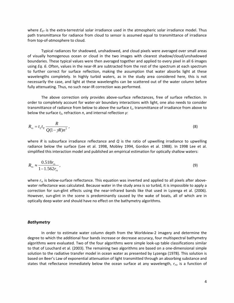
1

Derivation of bathymetry from multispectral imagery in the highly turbid waters of Singapore’s south islands: A comparative study

James F. Bramante, Durairaju Kumaran Raju, Sin Tsai Min Tropical Marine Science Institute, National University of Singapore

Abstract

Four algorithms for the determination of bathymetry from multispectral imagery were utilized with new 8-band images from DigitalGlobe’s Worldview-2 satellite. All four were evaluated for accuracy in Singapore’s extremely turbid coastal waters and were used to evaluate the effects of Worldview-2’s additional four multispectral bands. Of the four, the linear band algorithm developed by Lyzenga et al. and a comparative classification algorithm performed best, with normalized RMSE of 0.229 and 0.313 meters, respectively. The additional four bands provided by Worldview-2 decreased RMSE by 9% and 27% for these two algorithms, respectively. Possibly due to the domination of particle backscatter over pigment absorption in these turbid waters, the linear ratio algorithm developed by Stumpf et al. was found lacking. Analysis found that the usual relationship between ratios of low absorption to high absorption bands and depth does not hold for these waters, likely due to backscatter dominating leaving-water signals, masking relative absorption effects. High turbidity with secchi disk depth of 2 meters limited analysis to shallow reefs and coastline, and may have impacted sensitivity of the bathymetric algorithms.

Introduction

Accurate and high-resolution bathymetric data is a necessity for a wide range of coastal oceanographic research, but especially when studying the environmental health of benthic habitats, especially in areas that are often disturbed by human and natural phenomena. Active sensing methods, such as ship-based soundings and LIDAR can be unwieldy and expensive. Ship-based soundings often have very low spatial resolution and have trouble navigating shallow waters (Lyzenga et al. 2006). LIDAR, with its reliable accuracy and high resolution, is still too expensive for many applications, especially when updates to a bathymetric dataset are required with any frequency. Thus, passive remote sensing systems are an attractive option for sea depth determination.

Several broad approaches have been applied to this passive determination. Recently, inversion and optimization of quasi- or semi-analytical algorithms has been used with hyperspectral imagery to determine water properties and/or depth (Albert and Gege 2006, Brando and Dekker 2003, Lee et al, 2002, Maritorena et al. 2002, Gould et al. 2001, Lee et al. 1999). In particular, the semi-analytical model produced by Lee et al. (1998/1999), based on a model by Maritorena et al. (1994), has shown promise in accurately determining many constituent concentrations along with depth (Brando et al. 2009, IOCCG 2006, Cannizzaro and Carder 2006, Carder et al. 2005). Comparative approaches with look-up tables have also been used with accurate depth and constituent determination (Mobley et al. 2005, Louchard et al. 2003). However, there are no commercially available hyperspectral satellite platforms with a spatial resolution comparable to many multi-spectral satellites. Instead, high-resolution hyperspectral images must be acquired with aircraft or shipboard platforms, the use of which can be expensive, especially when planning for multiple surveys (Canizzaro and Carder 2006). In addition, processing of hyperspectral data is often computationally expensive, making multispectral images an attractive alternative.

2

When using multispectral imagery, empirical approaches are primarily used to derive bottom depth (Lyzenga et al. 2006, Stumpf et al. 2003, Philpot 1989, Lyzenga 1985). One of the major constraints in accuracy of these empirical approaches, when compared to hyperspectral derivations, is spectral resolution, either for comparison with look-up tables or accounting for variable water quality and bottom properties. With only 4 bands in the visible and near infrared spectrum, most multispectral satellites are unable to account for too many unknown parameters in radiative transfer models. However, DigitalGlobe just launched a multispectral satellite, Worldview-2, with 8 bands in the V-NIR spectrum, including a second band in the lower blue wavelength range, which could prove invaluable in coastal research for its greater depth penetration and the possibility of greater particle and pigment discrimination (Hoepffner and Zibordi 2009). This paper aims to evaluate several depth-determination algorithms for the new Worldview-2 imagery in the extremely turbid coastal waters surrounding Singapore. The algorithms themselves will be compared for accuracy and an assessment will be made on how the additional multispectral bands affect accuracy in general.

Background

Atmospheric Correction

Most common atmospheric correction regimes for satellite imagery involve using premeditated empirical field measurements or expensive radiative transfer modeling software. With persistent cloud cover over Singapore, the former is difficult and the investigator had no access to the latter. Lacking concurrent field measurements, ground targets of known reflectance, and the models necessary for radiative transfer theory-based corrections (Gao et al. 2009), the cloud shadow method outlined by Lee et al. (2005) was considered sufficient for the purposes of this comparative study. This method was considered especially effective because of clearly delineated opaque clouds, cloud shadow, and sunlit open waters in close proximity in two of the six images. The theory behind these atmospheric corrections and corrections for the air-water interface are outlined below.

The total radiance measured at sensor, here determined from digital number values using DigitalGlobe’s specified absolute calibration factors for each band, is generally understood to be the sum of path radiance due to Rayleigh and aerosol scattering and water-leaving radiance after atmospheric transmittance, all as a function of wavelength, or:

)()()( λλλ Wpatht LtLL ×+= , (1)

where t is the transmittance from surface to sensor and Lpath is radiance due to light scattered into the sensor from adjacent areas. Wavelength dependence for optical terms (denoted by λ) is omitted for brevity hereon, except where needed for clarity. Remote sensing reflectance at the ocean surface is defined as:

d

Wrs E

LR = , (2)

3

where Ed is downwelling spectral irradiance at the surface, and the surface is not considered Lambertian. Thus, to determine Rrs and correct for atmospheric distortions we must first evaluate path radiance, path transmittance, and downwelling solar irradiance.

The cloud shadow model, developed by Reinersman et al. (1998), assumes that radiance leaving pixels shadowed by a compact, opaque cloud results from diffuse skylight reflected off the water’s surface or scattered beneath it:

rsdiffpathsh REtLL ××+= , (3)

where Ediff is the diffusely scattered irradiance illuminating the shadowed pixels. If we assume that a.) the path radiance is spatially homogenous over a small area encompassing shadowed and neighboring unshadowed pixels, and b.) the ocean water’s inherent optical properties, and thus reflectance (Gordon et al. 1988), are uniform over the same area, we can calculate path radiance using at-sensor radiances for neighboring shadowed and unshadowed pixels. Specifically, if we define radiance in a neighboring unshadowed pixel as

rsdpathne REtLL ××+= (4)

we can determine that:

d

diff

shnenepath

EE

LLLL−

−−=

1

)( (Lee et al. 2005) (5)

The ratio of diffuse to total solar irradiance,d

diff

EE

, was estimated using the atmospheric solar irradiance

model created by Gregg and Carder (1990), with absorption coefficients of atmospheric constituents taken from Bird and Riordan (1986). Although the irradiance was calculated over a wide range of wavelengths at single-nanometer resolution, it was consolidated into averaged, WV2-equivalent bands using spectral response curves provided by DigitalGlobe. Once path radiance is known, t is estimated using radiance reflected from the top of the cloud. Since cloud-top radiance is defined identically to Eq. 4, if we assume a value for cloud remote sensing reflectance we can derive t*Ed and finally Rrs for each pixel as:

rsCloudpathcloud

pathtrs R

LLLL

R ×−

−=

)( (6)

Lee et al. defined RrsCloud as a spectrally constant value determined somehow through absolute cloud radiance. Here it was instead assumed to be a Lambertian reflector with:

ET

cloudrsCloud E

LR π= , (7)

4

where EET is the extra-terrestrial solar irradiance used in the atmospheric solar irradiance model. Thus path transmittance for radiance from cloud to sensor is assumed equal to transmittance of irradiance from top-of-atmosphere to cloud.

Typical radiances for shadowed, unshadowed, and cloud pixels were averaged over small areas of visually homogenous ocean or cloud in the two images with clearest shadow/cloud/unshadowed boundaries. These typical values were then averaged together and applied to every pixel in all 6 images using Eq. 6. Often, values in the near-IR are subtracted from the rest of the spectrum at each spectrum to further correct for surface reflection, making the assumption that water absorbs light at these wavelengths completely. In highly turbid waters, as in the study area considered here, this is not necessarily the case, and light at these wavelengths can be scattered out of the water column before fully attenuating. Thus, no such near-IR correction was performed.

The above correction only provides above-surface reflectances, free of surface reflection. In order to completely account for water-air boundary interactions with light, one also needs to consider transmittance of radiance from below to above the surface tL, transmittance of irradiance from above to below the surface tE, refraction n, and internal reflection γ:

2)1( nRQRttR ELrs γ−

= , (8)

where R is subsurface irradiance reflectance and Q is the ratio of upwelling irradiance to upwelling radiance below the surface (Lee et al. 1998, Mobley 1994, Gordon et al. 1988). In 1998 Lee et al. simplified this interaction model and published an empirical estimation for optically shallow waters:

rs

rsrs r

rR562.11

518.0−

≈ , (9)

where rrs is below-surface reflectance. This equation was inverted and applied to all pixels after above-water reflectance was calculated. Because water in the study area is so turbid, it is impossible to apply a correction for sun-glint effects using the near-infrared bands like that used in Lyzenga et al. (2006). However, sun-glint in the scene is predominantly caused by the wake of boats, all of which are in optically deep water and should have no effect on the bathymetry algorithms.

Bathymetry

In order to estimate water column depth from the Worldview-2 imagery and determine the degree to which the additional four bands increase or decrease accuracy, four multispectral bathymetry algorithms were evaluated. Two of the four algorithms were simple look-up table classifications similar to that of Louchard et al. (2003). The remaining two algorithms are based on a one-dimensional simple solution to the radiative transfer model in ocean water as presented by Lyzenga (1978). This solution is based on Beer’s Law of exponential attenuation of light transmitted through an absorbing substance and states that reflectance immediately below the ocean surface at any wavelength, rrs, is a function of

5

bottom albedo rB, reflectance of an infinitely deep water column rW, the sum of the upwelling and downwelling diffuse attenuation coefficients of light α, and depth h:

hWBWrs errrr α−−+= )( (10)

When applied to multispectral imagery, rW is often defined as the average below-surface reflectance over optically deep water (typically, that which is greater than 30 meters deep). When this model is inverted to find depth, the accuracy is mostly predicated on the values of bottom albedo and attenuation coefficients used. If this algorithm is applied to an entire image, any heterogeneity in water quality or bottom type will cause large errors in the output. This paper examines two algorithms used to account for such heterogeneity.

Linear Band Model

In his 1978 paper, Lyzenga attempted to account for variability in bottom type by using multiple spectral bands and a rotational matrix. First he defined a variable, Xj, for each of bands 1 – N as:

)ln( Wjjj LLX −= , (11)

where Lj is the above-surface radiance in band j and Lwj is averaged deep-water radiance. The radiances were log-transformed to create a linear relationship between input radiance and depth. Deep-water radiance was used to account for reflection due to surface effects and volume scattering in the water column and was assumed to result mainly from external water reflection, including sun-glint effects, and atmospheric scattering. Secondly, he used a rotational matrix, similar to principle components analysis, to account for depth-independent variability in radiance values between bands. He defined N variables as:

∑==

N

i jiji XAY1

, (12)

where Aij is the i-th variable in the rotational matrix for band j. This produced N – 1 depth-independent variables that could be used as indices of bottom type, and 1 variable, YN that had a linear relationship to depth and was used for bathymetric determination. Although this algorithm accounted for bottom type variability and did not require any existing depth measurements, it failed to account for any heterogeneity in water column properties across an image. This algorithm was updated by Lyzenga in 1985, and again in 2006 by Lyzenga et al., to account for water quality heterogeneity, finally modeling depth as:

∑ =−=

N

j jjo Xhhh1

ˆ , (13)

where ho and each hj are constants defining a linear relationship between Xj, again defined as above, and depth. ho and all of h1-hj are determined through multiple linear regression between a set of known depths and the log-transformed radiances found at those depths. Because radiance is converted to reflectance using the same irradiance values throughout an image, the above relationship holds if one uses log-transformed reflectances instead of radiance, as was done in this paper for consistency among different methods. Lyzenga showed that theoretically this algorithm should account for heterogeneity in

6

bottom type and water quality and still achieve accurate results (RMSE of 2.3 m for depths up to 20 meters in the 2006 validation). Theoretically, the number of significantly different bottom types and water masses for which this algorithm accounts is directly proportional to the number of bands used, implying that Worldview-2 imagery, with 8 bands, should produce more accurate results over heterogeneous waters than conventional multispectral satellites.

Linear Ratio Model

In 2003, Stumpf et al. published an alternative model for determining bathymetry that better accounts for water turbidity. The primary motive for developing this new model involved one of the major weaknesses of the Linear Band model. Some benthic communities are highly absorbing, especially in the blue and green spectral region. Closely packed sea grass and macroalgae can absorb enough light that when the deep-water signal is subtracted from total radiance as outlined above, the resulting signal is negative, resulting in a non-real number when log-transformed. In addition, in especially turbid waters frequented by large boat traffic, as with Singapore, deep-keeled vessels and sea bottom dredging can raise suspended sediment levels in near-surface deep waters, resulting in a much higher deep-water signal across the V-NIR spectrum and overestimated depths in shallower areas.

Stumpf et al. base their model on the same simplified one-dimensional radiative transfer solution as Lyzenga et al. and also use a log-transform to linearize the relationship between band spectral values and depth. Instead of using a multiple linear regression with band radiances or reflectance, Stumpf et al. used a simple linear relationship between the ratio of reflectances in two bands and depth. Specifically, water absorbs light differently throughout the spectrum and log-transformed reflectance should decrease linearly with depth. Low-absorption bands will have reflectance values that decrease with depth more slowly than high-absorption bands. Thus, the ratio of a low-absorption band reflectance to high-absorption band reflectance should display a linear increase with depth when both are log-transformed. Thus:

)ln()ln(ˆ

1rsLO

rsHIo nr

nrhhh += , (14)

where ho is an offset for zero depth as in Lyzenga's model, h1 is a tunable constant defining the slope of the relationship between the ratio and depth, and n is a large constant used to ensure positive log values and a linear response. The value of n was set to 1000 throughout this investigation, as variation in n has been shown to have no significant effect on estimated depth (Stumpf 2003). This model assumes that changes in bottom reflectance are either equal in both bands or affect the ratio insignificantly relative to depth, resulting in relatively constant ratios over different bottom types and constant depth. In Stumpf et al.'s paper they compare this ratio-transformed method to the Linear Band method, using LIDAR-derived depths to perform the latter multiple linear regression and nautical chart derived depths to tune the former linear relationship. Both methods produced comparable results for their study area, with maximum normalized RMSE below 0.6 up to 25 meters depth and 0.3 up to 15 meters depth. Although only two bands are used in the ratio-transformed model, it has been shown that the extra bands provided by Worldview-2 may better account for depth (Loomis 2009). Preliminary investigation for this paper showed agreement, with ratios of the “coastal blue” band to the “yellow” band especially having greater correlation with depth than the more customary blue-to-green ratios.

7

Classifications

In addition to the two algorithms based on an optical model of ocean depth and bottom type, two classifications using spectral look-up tables (LUT) were performed. The first classification, similar to that of Louchard et al. (2003), simply compared each reflectance spectrum in an image to an LUT of sample spectra using a linear least squares approach. Unlike in Louchard et al., the sample spectra were taken from image pixels with known depth, and not simulated. The accuracy and validity of any classification is dependent on the separability of the classification input variable or property and its relationship to the physical property defining unique clusters (Gordon 1994). In this paper, the physical property is depth and the classification input property is reflected solar radiation. The strong relationship between these two properties and the separability of the latter have been extensively validated (Hochberg et al. 2003, Lee et al. 1998, Maritorena et al. 1994). However, as discussed above, there are other properties, such as water quality and bottom type, that also strongly influence spectral signal and can confound its relationship with depth (as when highly absorbing sea grass causes overestimation of depth based on upwelling radiance). In order for a classification using an LUT to be accurate, the LUT must account for these confounding factors as well as depth. Specifically, a spectral library like the LUTs used must contain spectral signatures related to each depth over each combination of water mass and bottom type. The spectral LUT data used in this investigation were collated from nautical chart sounding depths that were taken irrespective of bottom type and water quality. It is assumed that with a large enough training dataset collected randomly with respect to these confounding variables the LUTs should sufficiently account for all water column regimes and bottom types found in the study area. The accuracy of the classification is predicated heavily on the accuracy of this assumption.

Because the spectral look-up tables used in this investigation were small enough to likely cause significant errors in the band-comparison classification, a second classification was performed using an LUT of log-transformed band ratios. As with the Linear Ratio model, band ratios should account for much of the variability in water quality and bottom type and represent variability in depth more completely. When used in a classification, this could make up for the error inherent in a small training set, assuming spectral band ratios change significantly more with depth than with other variables. However, the limiting of spectral signals (from N bands to at most N/2 band ratios) for comparison could make this classification more inaccurate than a simple band-comparison.

Study Area

The study area examined in this investigation extends roughly 8 km by 10 km south of the Singaporean mainland, encompassing several islands and coral patch reefs. DigitalGlobe Worldview-2 satellite imagery acquired for the site were tiled into six sections and given row/column designations. That imagery can be found in Figure 1 displayed as a true-color image with bands 5, 3, and 2 (conventional red, green, and blue bands). The images will be individually referred to by their row/column designations as displayed in Figure 1 for convenience. Images R1C1 through R2C2 contain three large islands, one smaller island, and several patch reefs. The northernmost island in R1C1 is Pulau Bukom, used exclusively by Shell for oil refinement and petrochemical manufacture. The large island just to the south of it is Pulau Semakau, consisting mostly of land reclaimed using landfill waste from the mainland. The northwestern portion of Semakau is characterized by natural forest and mangroves along the coast. The third large island, mostly encompassed in R2C2, is Pulau Sebarok, used as an oil storage

8

and refueling port. Fringe reefs exist along the western edge of Pulau Semakau and between the two land segments of Pulau Jong, the small, mostly untouched island just northwest of Sebarok. There are also three patch reefs in this area partially exposed during low tide, one just north of Semakau, another between Jong and Bukom, and one protected by a pier off of Sebarok in R2C2. Although the region of water surrounded by these islands sees relatively less traffic, the waters bordering this area are heavily trafficked by large tankers and shipping vessels. This traffic, exemplified by the many large vessels visible in R1C2, along with sea bottom dredging near the mainland northwest of R1C1 stir up vast amounts of suspended sediment. Secchi disk measurements placed in-water visibility at 2 meters the day after the WV2 images were taken, a typical value for Singapore’s “dry” season. Image R1C3 is dominated by Sentosa Island in the north, Pulau Tekukor in the center of the image and two islands called The Sisters further south, all of which are used for mainly recreational purposes and thus have some small-boat traffic. Sentosa’s beaches facing the south are primarily artificial and harbor no known reefs or significant benthic communities. The smaller islands in R1C3, including the tip of St. John’s Island to the east, are bordered by fringe reefs. When validating the depth calculations, most attention will be paid to depth of the water columns above reefs and small island bays. While most of the reefs visible in the image are intertidal and therefore very shallow, depth increases steeply from the edges of the patch and island reefs, dropping to 5 and 10 meter depths within 5 meters distance.

Materials and Methods

Worldview-2 is a new satellite imaging platform recently launched in October, 2009 by DigitalGlobe, Inc. WV2 produces panchromatic images with roughly 0.5 m resolution (after US governmental restrictions) and 8-band multispectral images with 2 m resolution at nadir. The 8 multispectral bands include 4 conventional visible and near-infrared bands common to multispectral satellites (wavelengths in nanometers)– Blue (450-510), Green (510-580), Red (630-690) and Near-IR1 (770-895) – as well as 4 new bands – Coastal (400-450), Yellow (585-625), Red Edge (705-745), and Near-IR 2 (770-895). WV2 images were acquired for the study area on April 27th, 2010 during mid-high tide. In the images there is significant cloud cover and haze, especially in the northern halves of R1C1 and R1C2. R1C2 also displays a significant amount of large shipping vessel traffic. At the time the image was taken, visibility measured at 6.9 km, temperature at 33° C, relative humidity at 72%, and wind speed at a high 6 m/s. Atmospheric data were collected from weather stations surrounding the study area and extrapolated to the exact time of day using historic hourly averages for that month. The WV2 images were orthorectified and tiled by DigitalGlobe, with no visible errors. The cloud shadow atmospheric correction was applied to each image, but haze was still visible after correction. Masks of each image were made to exclude pixels of land, cloud, cloud-shadow, and deep haze from the calculations. These masks were created using boundary values of bands 2 and 8, resulting in good fits for most of the images, but patchiness in R1C1 and R1C2 due to the prevalent haze.

Bathymetry training data for the algorithms and look-up tables was taken from an electronic nautical chart (ENC), provided by Singapore Marine and Port Authority (MPA). All data points in this set were acquired using echo-sounder and multi-beam sonar platforms in July 2008. The data (hereon referred to as ENC08) were displayed using ArcGIS and their point-value positions were associated with the pixel of WV2 image in which they were located. Look-up tables and training sets were then constructed using the depths from ENC08 and the 8-band spectral values from their corresponding image pixels. Care was taken in choosing training data to avoid depth data located in cloud or cloud-shadowed pixels. The depths were corrected for tide by adding a tidal height of 0.9 meters,

9

Stud

y A

rea

– Si

ngap

ore

Sout

h Is

land

s

Figu

re 1

: Mos

aic

of th

e or

igin

al s

ix W

orld

view

-2 im

ages

enc

ompa

ssin

g th

e st

udy

area

, with

out

atm

osph

eric

cor

rect

ion.

Red

line

s de

linea

te im

age

tiles

as

proc

ured

from

Dig

italG

lobe

.

10

extrapolating from hourly tide tables calculated for Pulau Bukom and Sentosa by Singapore MPA. Even after taking tidal height into account, however, some depths from ENC08 indicated that locations over the patch reefs were above water, when analysis of the image clearly demonstrated this to not be the case. Depths reported in these areas may be prone to greater inaccuracy due to the inability of ships making sounding measurements to traverse very shallow water. Depths indicated as above-water were removed from the training and validation data sets, which may have led to greater error over very shallow reefs.

For the LUT classification algorithms, two-thirds of the ENC08 depth values were used for look-up and one-third reserved for validation. For the empirical algorithms, all ENC08 depth data were used for calculation of coefficients in order to have the greatest representation of variance possible for overall accuracy. Because the study area waters exhibited such high turbidity and low visibility, it was deemed unnecessary to include depth data for optically deep waters where radiance could be assumed wholly the result of volume and residual atmospheric scattering. Training sets for the LUT comparisons were restricted to depth values 5 meters and shallower to speed up computation. For each of the empirical algorithms, coefficients were separately tuned to depths of 5m, 3m, and 2m, results for each run used and compared separately. The ENC08 data represented depths greater than 5 meters more completely than shallower depths, and below 1 meter there was relatively little data. The dearth of data at these depths was most likely a major source of error in the following depth estimations.

Because all ENC08 training data was used to calculate coefficients for the empirical algorithms, a second bathymetry dataset was obtained to perform validation independent of initial training values. This second dataset was extracted and corrected from an electronic navigation chart constructed in 2004 (ENC04) in the same manner as ENC08. It contained slightly higher spatial resolution data than ENC08, and all of its values were collected using multi-beam sonar. Although it is possible depths may have changed slightly between 2004 and 2008, it was assumed that the larger, independent dataset would provide more robust analysis for comparison between algorithms and between multispectral band combinations. After an algorithm had been applied across the entire study area, validation depths were extracted from the images using coordinates from ENC04 and compared to ENC04 depths for accuracy and precision. After comparing the two datasets for any obvious discrepancy, ENC04 was also used for validation purposes with the classification algorithms, discarding the initial ENC08 validation dataset.

The Linear Band algorithm was slightly modified for the current study. Because the area of interest is so turbid and impacted by large vehicle traffic, it would be inaccurate to assume that deep-water signals are due mostly to atmospheric scattering and surface reflection. In fact, highly absorbing benthic communities in shallow waters resulted in lower reflected signals over very shallow water than over deep water for some bands in the image. Because atmospheric corrections accounting for surface reflection and sky radiance were made across every image, it was deemed unnecessary to also subtract out deep-water signals. Instead, the log-transformed radiance was defined as in Stumpf et al. (2003):

)ln( rsj nrX = (15)

where n = 1000 was used for consistency between algorithms, with no detectable difference between depths modeled with and without the constant, and only the base coefficient, ho, being affected. This study also briefly evaluated the relative worth of using NIR bands in these computations, considering NIR signals are assumed to be mostly the effect of water column scattering and could therefore result in

11

unwanted noise. Including the NIR bands resulted in small but significant decreases in RMSE on the order of 0.001 meters, and they were included in this model. For comparison of WV2 bands with typical multispectral bands, the above algorithm was run using all 8 WV2 bands and again using only the 4 WV2 bands typifying most multispectral platforms (Blue, Green, Red, and Near-IR1). The results of these two runs were then compared.

The Linear Ratio algorithm was used unchanged from the theoretical form outlined above. Band ratios were chosen based on calculated correlation with depth in each training set. Coefficients of correlation were calculated for each band pair and depth, and the band pair with greatest correlation was used for further analysis. Results obtained using less correlated band ratios corroborated the use of coefficient of correlation as a valid measure of suitability. Comparison with typical multispectral bands was difficult, as the best band ratio for both the 3-meter and 2-meter datasets was Blue-to-Green. This made a realistic comparison using the additional WV2 bands impossible with the given training datasets.

LUT classifications were performed as outlined above. Each pixel in an image was compared to representative pixels in an LUT, its closest match calculated using least-squared error. For the ratio classification using all 8 WV2 bands, the three ratios Coastal-to-Green, Coastal-to-Yellow, and Coastal-to-Red were calculated and used for comparison. For the 4 band ratio classifications, the three ratios Blue-to-Green, Blue-to-Red, and Blue-to-Near IR1 were used.

12

0

0.5

1

1.5

2

2.5

0 0.5 1 1.5 2 2.5

Mod

eled

dep

th (m

)

0

0.5

1

1.5

2

2.5

0 0.5 1 1.5 2 2.5

Mod

eled

dep

th (m

)

Sounding depth (m)

0

0.5

1

1.5

2

2.5

0 0.5 1 1.5 2 2.5

Sounding depth (m)

a.

c.

0

0.5

1

1.5

2

2.5

0 0.5 1 1.5 2 2.5b.

d.

Figure 2: Modeled vs. Actual depth for 8-band algorithms. a.) is Linear Band, b.) is Linear Ratio, c.) is Band Classification, and d.) is Ratio Classification. The dotted lines represent perfect fit.

13

Line

ar B

and-

Det

erm

ined

Bat

hym

etry

Depth (m)

Figu

re 3

: Bat

hym

etry

der

ived

usi

ng L

inea

r-Ba

nd a

lgor

ithm

tune

d to

2 m

eter

s. N

ote

that

dep

th v

alue

s of

-1 m

indi

cate

pix

els

mas

ked

out b

ecau

se o

f clo

ud, c

loud

-sha

dow

, lan

d, o

r thi

ck h

aze.

The

nor

thw

este

rn p

ortio

n of

the

imag

e is

ove

r-m

aske

d, p

roba

bly

due

to s

uspe

nded

sed

imen

t ref

lect

ed s

igna

ls c

onfu

sed

as c

loud

/thi

ck h

aze

sign

al w

hen

deve

lopi

ng th

e sp

ectr

al m

asks

. N

ote

also

the

deep

wat

er c

lass

ified

as

haze

in th

e ce

nter

-sou

th.

This

ano

mal

y is

due

to in

finite

log

valu

es d

urin

g de

riva

tion,

des

pite

the

corr

ectin

g co

nsta

nt n

. In

this

imag

e, d

epth

val

ues

over

1.4

m w

ere

cons

ider

ed o

ptic

ally

dee

p an

d di

spla

y lim

ited

to v

alue

s be

low

1.4

m.

Not

e al

so th

at d

espi

te th

is c

utof

f, th

ere

are

still

som

e de

ep-w

ater

pix

els

estim

ated

as

less

than

1.4

m d

epth

.

14

Results and Discussion

The results of the algorithms produced for the LUTs with depths ≤ 2 meters and coefficients tuned to 2 meters, using all eight WV2 bands, are displayed in Figure 2. It is evident that even the use of ENC04 data for validation provides few data at this depth, although some data points are hidden beneath others with the same value when displayed, especially in the classification graphs. The Linear Band model (Fig. 2a) produces results that fit well relative to results in Stumpf et al. (2003) and Lyzenga et al. (2006). It is still hard to compare results with those reported in these papers because they don’t report such shallow derived depths. However, with a normalized RMSE of 0.229 meters, the depth derivation here performs better than the corresponding derivation at 2.5-5 meters as reported by Stumpf et al. The Linear Ratio model (Fig. 2b) did not perform so well. While it has a similar precision, indicated by a normalized RMSE value of 0.260 meters, the data displays less overall accuracy, as shown in its deviation from perfect fit. Plotted derivations using the Linear Ratio algorithm seem almost independent of true depth between 0.5-1 m and 1.6-2 m. The band classification (Fig. 2c) was less precise than either with a normalized RMSE of 0.313 meters. Compared to the similar approach by Louchard et al. (2003), this band classification performs worse, with a median error of 25%, but this is more accurate than the Linear Band algorithm. The results produced by the ratio classification (Fig. 2d) perform much worse, with slightly higher RMSE and median error, but nearly 30% greater average error. These results may indicate that empirical algorithms perform better than LUT classification when considering such shallow depths and small initial training sets.

Figure 4 displays the results for the algorithms performed with just the conventional 4 multispectral bands. It is obvious from the plots alone that the band classification performs much worse with only 4 bands to compare between the LUT and image, having a normalized RMSE of 0.428 meters and 40% worse median accuracy. The 4-band Linear Band algorithm has slightly worse precision than its complement with a normalized RMSE of 0.252 meters and 10% worse average accuracy, though it has insignificantly better median error. As stated earlier, a 4-band comparison of the Linear Ratio algorithm was not possible for these depths because the ratio used was conventional Blue-to-Green. The 4-band ratio classification performed better than its 8-band counterpart. This investigation found that these results held even when replacing the Coastal-to-Green ratio with Blue-to-Green in the 8-band algorithm. Although individual ratios involving the coastal and yellow band were more highly correlated to depth than ratios using only conventional multispectral bands, the wider separation in wavelength between the conventional bands may account for more variation with depth, resulting in more accurate classification. The band classification produces more accurate results with a small trade-off in computation time. RMSE and median percent error for all derivations are displayed in Figures 5 and 7.

The calculations performed using LUTs and coefficients tuned to depths greater than 2 meters proved significantly less accurate than those calculated up to 2 meters and are not examined here.

15

-0.5

0

0.5

1

1.5

2

0 0.5 1 1.5 2 2.5

Mod

eled

dep

th (m

)

Sounding depth (m)

0

0.5

1

1.5

2

2.5

0 0.5 1 1.5 2 2.5

Sounding depth (m)

0

0.5

1

1.5

2

2.5

0 0.5 1 1.5 2 2.5

Mod

eled

dep

th (m

)

Sounding depth (m)

Figure 4: Modeled vs. Actual depth for 4-band algorithms. a.) is Linear Band, b.) is Band Classification, and c.) is Ratio Classification

a. b.

c.

16

Although the 8-band Linear Band algorithm and band classification do perform relatively well for depths below two meters, all of the algorithms considered in this study showed substantial error. There are several possible sources for this error, and we will analyze them here. First, the time difference between the first and second bathymetry datasets used for training and validation may result in perceived error due to changes in depth over time. However, the algorithms are not significantly more accurate when judged solely on data from ENC08. Another possible source of error is the atmospheric correction used. Incorrect estimations of gas and aerosol absorption coefficients in the atmosphere could cause some error, but it is improbable that these estimates would be inaccurate enough to cause significant error. To test whether the water-air boundary interaction equation taken from Lee et al. (1998) held true for the study area, a second atmospheric correction was run without it and the results of bathymetry algorithms compared to these results, but there were no changes in precision or accuracy.

The training sets and LUTs used in this study are highly probable sources of error. The LUTs and training sets were statistically small due to the small size of bathymetry data from which they were extracted. If more extensive training sets were used, either with broader measured or simulated data, the accuracy of these algorithms might improve significantly. It is also possible that the relationships between depth and spectral signal utilized by these algorithms are simply not sensitive enough over such a small range of depths, leading to a baseline error equivalent to those reported here. A larger training and validation dataset, with greater representation at shallower depths, would help explore this possibility.

Assumptions made in the construction of the algorithm could also be sources of error.

Both of the empirical algorithms are based on the concept of exponential attenuation of light through water. Both algorithms also assume

that the main mechanism for this attenuation is absorption. Lyzenga et al.’s model initially makes this assumption through the subtraction of deep water values from reflectance values throughout an image. As Stumpf et al. pointed out, shallow water with highly-absorbing bottoms may have lower reflectance values than deep water with significant particle backscattering. This situation is exemplified by comparing reflectance over the sea grass beds and coral surrounding Pulau Semakau in R1C1 to deep water reflectance in R1C2 where traffic has significantly raised levels of suspended sediment, visible as plumes beneath the ocean surface. This study avoids the error caused in that assumption by leaving out the deep-water term, though this step most likely adds its own error as well. Stump et al.’s Linear Ratio algorithm implicitly assumes a water column is dominated by absorption when specifying ratios of high-to-low absorbing bands. In a regime as highly turbid as Singapore waters, particle backscattering may be the primary mechanism for attenuation. Since many ocean sediments scatter relatively equally across the V-NIR spectrum, ratios of differently absorbing bands may change less with depth than in an absorbing regime, flattening the linear relationship between depth and the log-transformed ratios. This

Figure 5: Comparison of root mean squared error for all of the algorithms.

0

0.1

0.2

0.3

0.4

0.5

0.6

0.7

0.8

0.9

Root

Mea

n Sq

uare

Err

or (m

)

RMSE

8-band

4-band

17

Band

-Cla

ssifi

ed B

athy

met

ry

Depth (m)

Figu

re 6

: Ban

d Cl

assi

ficat

ion-

deri

ved

bath

ymet

ry o

f the

stu

dy a

rea.

Pix

els

repo

rtin

g 0

dept

h ha

ve b

een

mas

ked

out b

ecau

se o

f the

pre

senc

e

of la

nd, c

loud

, clo

ud-s

hado

w, s

hipp

ing

vess

els,

or t

hick

haz

e. A

s in

Fig

ure

7, s

ome

of th

e no

rthw

este

rn c

orne

r of t

he im

age

has

been

ove

r-

mas

ked.

Not

e ho

w in

dee

p w

ater

(cla

ssifi

ed a

s ab

out 2

m),

wat

er m

asse

s w

ith h

igh

susp

ende

d se

dim

ent c

once

ntra

tions

are

cla

ssifi

ed a

s

rela

tivel

y sh

allo

w w

ith s

edim

ent p

lum

es v

isib

le s

tret

chin

g fr

om th

e sh

ippi

ng v

esse

ls in

the

cent

er o

f the

stu

dy a

rea

to th

e so

uthe

ast c

orne

r.

18

would decrease the accuracy and precision of the Linear Ratio model, and if backscattering dominates attenuation within the water column, it could be assumed that band ratios stay constant with changing depth. This possibility was analyzed and the inseparability of these ratios by depth, as displayed in Figure 8, seems to support the hypothesis that these waters are not absorbing regimes and may not be effectively analyzed by the Linear Ratio algorithm.

Bathymetric maps produced using the Linear Band model and band classification are displayed in Figures 3 and 6. Both algorithms delineate well between shallow water benthic habitats and optically deep water. The patch and fringe reefs are well defined in both images, including steep drop-offs to deeper water. The depths in Figure 3 show better transitions from shallow to deep water, with less speckle error and less sensitivity to bottom type over the Semakau fringe reefs and sea grass beds. Figure 3 only displays water with depth values equal to or shallower than 1.4 meters, waters classified as deeper than that considered optically deep. Figure 6 displays classification with unaltered and unrestricted values. In Figure 6, a large sediment plume, misclassified as shallower water, is visible stretching from the centrally located shipping vessels to the southeast corner of the study area. In Figure 3 this plume and other more localized plumes were also visible before restricting depth values to 1.4 meters.

2.8

3.3

3.8

4.3

4.8

5.3

5.8

2 2.5 3 3.5 4 4.5 5 5.5 6

ln(n

*Blu

e)

ln(n*Green)

Blue-to-Green Band Ratio

0.1 - 0.5 m

0.6 - 1 m

1.1 - 1.5 m

1.6 - 2 m

0

10

20

30

40

50

60

70

Med

ian

Perc

ent A

bsol

ute

Erro

r (%

)

Median Absolute Error

8-band

4-band

Figure 7: Comparison of median absolute error for all of the algorithms

Figure 8: Comparison of Blue-to-Green band ratios in Singapore shallow waters with respect to depth. Ratios appear inseparable by depth, especially below 0.5 meters.

19

Conclusions

Four algorithms used to determine water column depth using multispectral satellite images were examined in this paper. Because of the high turbidity of Singapore waters, this investigation was restricted to studying and deriving depths shallower than two meters. Within this narrow band of depth, it is difficult to obtain accurate results because of variable bottom type, instrument error, and inaccurate assumptions regarding the water column. Two of the algorithms have the potential to accurately determine shallow depth in highly turbid waters given sufficiently representative training data sets. The Linear Band algorithm modified from Lyzenga et al. (2006) obtained a normalized RMSE of 0.229 meters and a median error of 26%. A band classification using look-up tables obtained a normalized RMSE of 0.313 meters and a median error of 25%. The additional 4 V-NIR spectral bands provided by the Worldview-2 improved the Linear Band algorithm marginally, but decreased median error of the band classification from 65% to the 25% reported here. A classification using band ratios instead of raw band values achieved results comparable to the Linear Band algorithm. Although its data input requirements are the same as the more accurate band classification, its lower computation requirements may make it attractive after further validation. Another algorithm considered here, the Linear Ratio algorithm developed by Stumpf et al. (2003), may prove completely ineffective in waters where turbidity is the predominant factor defining attenuation in the water column. In order to achieve better results in the future, training sets should be constructed with more care given to representing a wide range of variance in bottom type and water column properties with statistically significant sample sizes at critical depths. Better quality images free of cloud cover and haze would allow for a more accurate assessment of bathymetry in Singapore, possibly removing most error affecting the classification methods. Using tide-linked bathymetric datasets with higher spatial coverage and vertical resolution may remove much of the error in these shallow depths for all of the algorithms considered.

References

Albert, Andreas and Peter Gege. (2006). “Inversion of irradiance and remote sensing reflectance in shallow water between 400 and 800 nm for calculations of water and bottom properties.” Applied Optics 45.10: 2331-2343.

Bird, Richard E. and Carol Riordan. (1986). “Simple Solar Spectral Model for Direct and Diffuse Irradiance on Horizontal and Tilted Planes at the Earth's Surface for Cloudless Atmospheres.” Journal of Climate and Applied Meteorology 25: 87-97.

Brando, Vittorio E., Janet M. Anstee, Magnus Wettle, Arnold G. Dekker, Stuart R. Phinn, and Chris Roelfsema. (2009). “A physics based retrieval and quality assessment of bathymetry from suboptimal hyperspectral data.” Remote Sensing of Environment 113: 755-770.

Brando, Vittorio E. and Arnold G. Dekker. (2003). “Satellite Hyperspectral Remote Sensing for Estuarine and Coastal Water Quality.” IEEE Transactions on Geoscience and Remote Sensing 41.6: 1378-1387.

Cannizzaro, Jennifer Patch and Kendall L. Carder. (2006). “Estimating chlorophyll a concentrations from remote-sensing reflectance in optically shallow waters.” Remote Sensing of Environment 101: 13-24.

20

Carder, Kendall L., Jennifer P. Cannizzaro, and Zhongping Lee. (2005). “Ocean color algorithms in optically shallow waters: Limitations and improvements.” Proceedings of SPIE 5885: 06.1-06.11.

Gao, Bo-Cai, Marcos J. Montes, Curtiss O. Davis, and Alexander F. H. Goetz. (2009). “Atmospheric correction algorithms for hyperspectral remote sensing data of land and ocean.” Remote Sensing of Environment 113: S17-S24.

Gordon, A.D. (1994). “Identifying genuine clusters in a classification.” Computational Statistics and Data Analysis 18: 561-581.

Gould, R.W. Jr., R. A. Arnorne, and M. Sydor. (2001). “Absorption, Scattering, and Remote-Sensing Reflectance Relationships in Coastal Waters: Testing a New Inversion Algorithm.” Journal of Coastal Research 17.2: 328-341.

Gregg, Watson W. and Kendall L. Carder. (1990). “A Simple Spectral Solar Irradiance Model for Cloudless Maritime Atmospheres.” Limnology and Oceanography 35.8: 1657-1675.

Hochberg, Eric J., Marlin J. Atkinson, and Serge Andrefouet. (2003). “Spectral reflectance of coral reef bottom-types worldwide and implications for coral reef remote sensing.” Remote Sensing of Environment 85: 159-173.

Hoepffner, N. and G. Zibordi. (2009). “Remote Sensing of Coastal Waters.” Encyclopedia of Ocean Sciences (2nd ed.): 732-741.

IOCCG (2006). “Remote Sensing of Inherent Optical Properties: Fundamentals, Tests of Algorithms, and Applications.” Lee, Z.-P. (ed.), Reports of the International Ocean-Colour Coordinating Group, No. 5, IOCCG, Dartmouth, Canada.

Lee, ZhongPing, Casey Brandon, Rost Parsons, Wesley Goode, Alan Weidemann, and Robert Arnorne. (2005). “Bathymetry of shallow coastal regions derived from space-borne hyperspectral sensor.” Oceans-IEEE: Oceans 2005 Proceedings 2160-2170.

Lee, Zhongping, Kendall L. Carder, and Robert A. Arnorne. (2002). “Deriving inherent optical properties from water color: a multiband quasi-analytical algorithm for optically deep waters.” Applied Optics 41.27: 5755-5772.

Lee, Zhongping, Kendall L. Carder, Curtis D. Mobley, Robert G. Steward, and Jennifer S. Patch. (1999). “Hyperspectral remote sensing for shallow waters: 2. Deriving bottom depths and water properties by optimization.” Applied Optics 38.18: 3831-3843.

Lee, Zhongping, Kendall L. Carder, Curtis D. Mobley, Robert G. Steward, and Jennifer S. Patch. (1998). “Hyperspectral remote sensing for shallow waters: I. A semianalytical model.” Applied Optics 37.27: 6329-6338.

Louchard, Eric M., R. Pamela Reid, Carol Stephens, Curtiss O. Davis, Robert A. Leathers, and T. Valerie Downes. (2003). “Optical Remote Sensing of Benthic Habitats and Bathymetry in Coastal Environments at Lee Stocking Island, Bahamas: A Comparative Spectral Classification Approach.” Limnology and Oceanography 48.1: 511-521.

21

Lyzenga, David R., Norman P. Malinas, and Fred J. Tanis. (2006). “Multispectral Bathymetry Using a Simple Physically Based Algorithm.” IEEE Transactions on Geoscience and Remote Sensing 44.8: 2251-2259.

Lyzenga, David R. (1985). “Shallow-water bathymetry using combined LIDAR and passive multispectral scanner data.” International Journal of Remote Sensing 6.1: 115-125.

Lyzenga, David R. (1978). “Passive remote sensing techniques for mapping water depth and bottom features.” Applied Optics 17.3: 379-383.

Maritorena, Stephane, David A. Siegel, and Alan R. Peterson. (2002). “Optimization of a semi-analytical ocean color model for global-scale applications.” Applied Optics 41.15: 2705-2714.

Maritorena, Stephane, Andre Morel, and Bernard Gentili. (1994). “Diffuse Reflectance of Oceanic Shallow Waters: Influence of Water Depth and Bottom Albedo.” Limnology and Oceanography 39.7: 1689-1703.

Mobley, Curtis D., Lydia K. Sundman, Curtiss O. Davis, Jeffrey H. Bowles, Trijntje Valerie Downes, Robert A. Leathers, Marcos J. Montes, William Paul Bissett, David D. R. Kohler, Ruth Pamela Reid, Eric M. Louchard, and Arthur Gleason. (2005). “Interpretation of hyperspectral remote-sensing imagery by spectrum matching and look-up tables.” Applied Optics 44.17: 3576-3592.

Philpot, William D. (1989). “Bathymetric mapping with passive multispectral imagery.” Applied Optics 28.8: 1569-1578.

Reinersman, Phillip N., Kendall L. Carder, and Feng-I R. Chen. (1998). “Satellite-sensor calibration verification with the cloud-shadow method.” Applied Optics 37.24: 5541-5549.

Stumpf, Richard P., Kristine Holdried, and Mark Sinclair. (2003). “Determination of Water Depth with High-Resolution Satellite Imagery Over Variable Bottom Types.” Limnology and Oceanography 48.1 Part 2: Light in Shallow Waters: 547-556.