DEPRECIATION - Australian Competition and Consumer … · FINAL 11 AUGUST 2008 DEPRECIATION PAGE 1...

REPORT

DEPRECIATION

Report by Henry Ergas

Prepared for: Mallesons Stephen Jaques

Date: August 2008

Concept Economics:27 Jardine Street, PO Box 5430 Kingston ACT 2604 Australia

FINAL

11 AUGUST 2008 DEPRECIATION PAGE ii

© Concept Economics Pty Ltd 2008 ABN 73 129 990 530 This work is copyright. The Copyright Act permits fair dealing for study, research, news reporting, criticism or review. Selected passages, tables or charts may be reproduced for such purposes provided the acknowledgment of the source is included. Permission must be obtained from Concept Economics’ Knowledge Manager, Shirley Carpenter on +61 2 8233 4090 or email [email protected].

FINAL

11 AUGUST 2008 DEPRECIATION PAGE iii

Disclaimer

Concept Economics and its author(s) make no representation or warranty as to the accuracy or completeness of the material contained in this document and shall have, and accept, no liability for any statements, opinions, information or matters (expressed or implied) arising out of, contained in or derived from this document or any omissions from this document, or any other written or oral communication transmitted or made available to any other party in relation to the subject matter of this document. The views expressed in this report are those of the author(s) and do not necessarily reflect the views of other Concept Economics staff.

11 AUGUST 2008 DEPRECIATION

FINAL

PAGE iv

Table of contents

1. INTRODUCTION 1 1.1. TERMS OF REFERENCE 1 1.2. SUMMARY OF FINDINGS 1 1.3. STRUCTURE OF THIS REPORT 4 1.4. SUPPORTING INFORMATION 5

2. THE REGULATORY BARGAIN 6 2.1. EXPECTATIONAL CAPITAL MAINTENANCE 6 2.2. ACCOUNTING SYSTEMS AND THE CHOICE OF COST BASE 2.2.1. Historical cost accounting 8 2.2.2. Current cost accounting and forward-looking costs 9 2.3. INCENTIVES FOR INVESTMENT 12 2.3.1. Risk of time inconsistency 12 2.3.2. “Inefficient” prices versus dynamic (investment) inefficiencies 14 2.4. CONCLUSIONS 15

3. DEPRECIATION AND EX ANTE CAPITAL MAINTENANCE 17 3.1. ECONOMIC DEPRECIATION 18 3.1.1. Economic depreciation and prices 18 3.1.2. Depreciation, revaluation, and obsolescence 19 3.1.3. Economic depreciation profiles 22 3.1.4. Measuring economic depreciation 28 3.2. ACCOUNTING DEPRECIATION 30 3.2.1. The accounting theory debate 30 3.2.2. Accounting depreciation profiles 31 3.3. DEPRECIATION IN A REGULATORY SETTING 33 3.3.1. The Invariance Proposition 33 3.3.2. Optimal depreciation policy 35 3.3.3. Competition and technical progress 37 3.3.4. Uncertainty and regulatory error 38 3.4. CONCLUSIONS 39

4. WHETHER THE DEPRECIATION APPROACHES ADOPTED BY TELSTRA AND THE ACCC ARE “REASONABLE” 41

4.1. THE STATUTORY CRITERION 41 4.2. DEPRECIATION IN THE TEA MODEL 43 4.2.1. Telstra approach 43 4.2.2. ACCC approach 44 4.3. ASSSESSMENT OF THE CHOICE OF DEPRECIATION

ROFILE 46 4.3.1. Whether straight-line depreciation is reasonable 46 4.3.2. Whether the tilted annuity approach is reasonable 48 4.4. CONCLUSIONS 54

APPENDIX A: TERMS OF REFERENCE 56

APPENDIX B: CURRICULUM VITAE FOR HENRY ERGAS 62

8

P

FINAL

11 AUGUST 2008 DEPRECIATION PAGE 1

1. INTRODUCTION

I am instructed that on 3 March 2008 Telstra submitted to the Australian Competition and Consumer Commission (“ACCC”) an ordinary access undertaking for Unconditioned Local Loop Service (“ULLS”). In support of the Undertaking Telstra relies, amongst other things, upon an engineering cost model known as the TEA Model, which it has developed for the purposes of calculating the total service long-run incremental cost (“TSLRIC”) of supplying ULLS.

I am instructed that the TEA model calculates the capital cost of deploying a current best practice Customer Access Network (“CAN”) and then calculates the required depreciation for that capital base. Depreciation is one component of the building block approach used to calculate the TSLRIC of supplying ULLS. For the purposes of calculating depreciation the TEA Model uses what is commonly referred to as a “straight line” depreciation (“SLD”) profile. Other components of the building block approach are added, then the sum of these components is levelised over time using an annuity formula. In contrast, the ACCC has in the past taken the view that a tilted annuity should be used to calculate the annual cost of depreciation for the purposes of calculating the TSLRIC of supplying ULLS.

1.1. TERMS OF REFERENCE

I have been asked by Mallesons Stephen Jacques (“Mallesons”) to provide:

1. my views as to whether application of commonly accepted economic theory would reasonably lead to the use of a tilted annuity to calculate depreciation, in the way that the ACCC has done in the past;

2. having regard to (1.) above, my views as to whether the ACCC’s use of the tilted annuity formula for depreciation achieves the stated objectives of Part XIC of the Act, in particular the statutory criteria relevant to ordinary access undertakings set out in sections 152AH and 152AB of the Trade Practices Act 1974;

3. in support of my views, a succinct survey of the relevant accepted economic literature in relation to the calculation of depreciation.

My instructions are contained in letters of instructions from Mallesons dated:

1. 5 June 2008; and

2. 26 June 2008.

Copies of these letters are contained in Appendix A of this report.

1.2. SUMMARY OF FINDINGS

ense, depreciation refers to the way in which certain kinds of long-lived assets fall in value (price) over their useful life. Depreciation charges are intended to recover total outlays for the capital equipment required to deliver a product or service. In this statement I am concerned with the structure of depreciation charges for the ULLS service.

In a general s

FINAL


The ACCC’s tilted annuity formula for depreciation has the effect of postponing – and putting at risk – cost-recovery for regulated assets.

e or expectational ust reasonably

r. If, in the ested, for

example, in Telstra, will not be returned to them, they will only make such funds available investment that

consumers.

capital being assured

ugh they may

In Australian regulation, there is generally no such guarantee, as regulators base charges ept of efficient costs with costs being periodically re-estimated.

cally nflicting

ver time, in particular in relation to how it values Telstra’s assets. by effectively

petition or substantial changes in circumstances may undermine cost recovery. For example, some

ly obsolete by a National Broadband Network incorporating Fibre to

HFC”) cable network is also a at in major metropolitan areas. Moreover, developments in HFC technology

ts own HFC. Finally, there is the prospect of m wireless services.

portant factor in ensuring expectational ustries with high capital intensity and very long lived assets, such

as telecommunications. The return of capital, i.e. depreciation, is a crucial component of issues looms

effect of

as long been an issue of concern both to economists and to accountants. There are significant differences between the “economic” and “accounting” approach to depreciation:

• The economic approach to depreciation seeks to mimic the pattern of asset prices that would be revealed in well-functioning markets for (aging) second-hand assets, and hence to reflect the opportunity cost of making asset services available.

In my opinion, a key element in any durable regulatory contract is ex antcapital maintenance. That is, if investors prudently invest a dollar, they mexpect both a reasonable return on, and the ultimate return of, that dollaalternative, investors perceive that there is a significant risk that funds inv

at a higher cost, if at all. In turn, higher funding costs would reduce the Telstra would choose to undertake, an outcome that would eventually harm

In some systems of regulation – notably pure “rate of return” regulation –maintenance is more or less guaranteed, with investors and regulated firmsof cost recovery. These systems do a good job of ensuring investment, thonot provide incentives for cost-efficiency.

on a “forward-looking” conc

Expectational capital maintenance poses challenges because of the risk of time inconsistency in regulation, a risk which is magnified when costs are periodiredetermined. That is, the regulator (in this case, the ACCC) may adopt coregulatory approaches oTime inconsistent policies harm shareholders’ interests if their capital is therereduced, and will ultimately harm consumers.

Expectational capital maintenance also poses specific challenges when com

part of Telstra’s copper loops and local network may be rendered effectivethe Government’s decision to buildthe Node (“FTTN”) architecture. Optus’ hybrid fibre coaxial (“competitive thremight lead Telstra itself to shift usage to iincreased competition fro

The setting of the capital charge is an especially imcapital maintenance in ind

the capital charge. Moreover, it is the component where timing of recoverylargest, as different ways of determining the capital charge may have thesignificantly deferring that return.

The proper approach to depreciation h

FINAL


• The accounting approach seeks to allocate the loss in value of an agingparticular periods of time and units of output, with less concern aboutopportunity costs. It has the advantage of greater verifiability, though aof the extent to which potentially relevant oppo

asset to reflecting notional

t a cost in terms rtunity costs are being measured.

f depreciation s

iscount rates, e, in turn, determined

et). In some (unusual) ly “back-

t’s useful life. However, and-side)

omic lier years of the

“Invariance ectational

). For any ch a way that the unted at the

of capital) is zero at all points in time over the useful life of the asset. This

omic literature that the Invariance Proposition ut the

of obsolescence, sed” as a result of

inty about future preciation use they

er the cost of its

e economic iods and units of cluding

lated service arges (including

of them mptions.

The statutory test in sections 152AH and 152AB of the Trade Practices Act 1974 asks whether an approach is reasonable. This does not mean that it is the only approach that is reasonable, but that it itself is reasonable.

Telstra applies a SLD profile to the asset categories required to produce the ULLS. SLD reduces the written down value of assets by an equal increment in each year of an asset’s useful life. As such, SLD can be viewed as a “compromise” between a front-loaded and a

To the extent to which an economic approach is adopted, the time profile ocharges depends on a number of factors, including the time-efficiency profile of the asset(the extent to which the asset’s productive capability “decays” as it ages), d

hich arand expectations of future changes in the value of the asset (wby demand and supply trends for the output produced by the assinstances, these combined factors can lead to a time profile that is effectiveloaded”, so that depreciation is greater in the later years of the assewhen assets physically deteriorate, where there is a risk of (technical or demobsolescence, and, in general, when future price trends are uncertain, econdepreciation is “front-loaded”, so that depreciation is greater in the earasset’s useful life.

In a regulatory context, and as demonstrated by Schmalensee in hisProposition”, there is a family of depreciation profiles that are consistent with expcapital maintenance (so that shareholders are “indifferent” between themparticular regulated asset, these depreciation profiles are determined in supresent value of the future income stream associated with the asset (discoregulated costcondition implies that investors are assured of full cost recovery.

However, it is widely recognised in the econonly holds under idealised conditions, and breaks down when assumptions aboregulated firm’s future revenues are more realistic: where there is a riskbecause (say) existing infrastructure can effectively be “bypastechnological innovations, and, more generally where there is uncertarevenues, including regulated revenues. In these circumstances, certain deprofiles, in particular back-loaded depreciation profiles are more risky, becaincrease the probability that the regulated firm will not be able to recovinvested capital in some circumstances.

In a regulatory setting, there may also be circumstances where no uniqudepreciation profile (that would match cost causality to particular time peroutput) exists. “Ramsey” pricing principles whereby regulated charges (indepreciation) are set to reflect the price sensitivity of consumers of the regucan then ensure full cost recovery. However, calculating such regulated chthe implicit depreciation component) involves numerous assumptions, manydifficult to test, and the results can be highly sensitive to these assu

FINAL


back-loaded depreciation profile. There are, however, a number of factors a front-loaded depreciation preferable from an ex ante capital maintenan

that would make ce perspective,

me, for ive and/or offer

e ACCC in the reater commercial

ings of the C competition, or

longer assured. As ely lead to

be offset by a cing Model

f return in Australia, s never been

tilted annuity

1.3

enance in the r. The ability of a

financial capital this is achieved

ng” accounting system to significant

ined, so that capital maintenance objectives may not be met. As a result, the time reciation “profile”) that is applied to a service provider’s

ignificance.

Section 3 examines economic and accounting approaches to depreciation. While economic reciation provides

iles are likely to may generate,

other factors) s, investors in a

depreciation profiles. This .

However, this “Invariance Proposition” breaks down when there is a risk that, for instance as a result of competitive or technological trends, the regulated firm cannot recover its (historical) investment expenditures (the Invariance Proposition resting, among other things, on the assumption that actual returns equal allowed returns, and that allowed depreciation sums to the asset’s original value).

Section 4 sets out my assessment of whether commonly accepted economic theory would reasonably lead to the use of a “tilted annuity” to calculate depreciation in the way that the

including risks of competitive bypass. These risks are likely to be rising over tiinstance, as wireless alternatives and HFC become more cost-effectequivalent or better service.

In contrast, a tilted annuity approach to depreciation as has been used by thpast imposes a high degree of back-loading and exposes investors to gand regulatory risk. If there is, at the same time, a risk that the future earnrelevant assets are reduced, for instance as a result of FTTN or HFbecause the asset is revalued, expectational capital maintenance is no a result, I would expect Telstra’s cost of capital to increase, which would likinefficiently low levels of investment. In principle, the resulting risk could higher rate of return, but that would be a departure from the Capital Asset Pri(“CAPM”), which is commonly applied to determine regulated rates oand which only rewards systematic risk. In practice, such an approach hataken in a regulatory context in Australia. As a result, I consider that a approach to depreciation is not reasonable.

. STRUCTURE OF THIS REPORT

This report is structured as follows.

Section 2 sets out the central importance of ex ante financial capital maintcontext of the “regulatory bargain” between a regulated firm and the regulatoregulated firm to attract the financing it requires to invest is premised onmaintenance, and the depreciation charge is the mechanism through whichin all accounting systems. However, in the context of the “forward-lookiadopted in Australian telecommunications regulation, investors are exposed risks of “time inconsistency” in regulation, particularly since costs are periodically redetermpattern of depreciation (or the depregulated assets is of particular s

depreciation is complex to derive in practice, the theory of economic depimportant insights about the circumstances when particular depreciation profemerge. Specifically, risks relating to the future earnings that a firm’s assetsincluding risks arising from technical or demand-side obsolescence (but also would lead to front-loaded depreciation profiles. Under idealised conditionrate-of-return regulated firm would be indifferent between differentis because the regulated firm is left financially neutral in net present value (“NPV") terms


FINAL

PAGE 5

CCC’s use of a tilted annuity formula for depreciation to be the case.

cantly back-loaded oking” accounting

h Telstra is recoup the cost of

investors in the and would prevent

ither in the nt with the objectives of

d relied on a uch as SLD) for

nable and more likely to achieve the objectives of the Act.

1.4

competition atters related

sisted Telstra in range of

ting and wholesale line

ork.

e Federal Court of rt.

Appendix B.

ACCC has done, and whether the Aachieves the stated objectives of Part XIC of the Act. I do not consider this The tilted annuity approach to calculating capital charges leads to a signifidepreciation profile where asset prices are increasing. Given the “forward-losystem applied by the ACCC, and given broader competitive trends to whicexposed, this approach magnifies the risk that Telstra would not be able toinvestments prudently undertaken. A regulatory bargain that does not assureregulated firm of ex ante financial capital maintenance is not sustainable,Telstra from attracting the funds it requires to invest. Such an outcome is neinterests of shareholders, nor of customers, and cannot be consistethe Act. Instead, an approach that locked in Telstra’s efficient asset base anmore transparent and less arbitrary (accounting) depreciation approach (scost recovery is more reaso

. SUPPORTING INFORMATION

I confirm that I have advised Telstra since the early 1990s on regulatory andissues, including analysing costing and pricing issues, access charging, and mto cost-recovery under the Universal Service Obligation. I have also asrespect of major ACCC inquiries and proceedings. These include advice on aservices, including ULLS, public switched telephone network (PSTN) originaterminating access services, local carriage service, line sharing service andrental, as well as the proposed fibre-to-the-node National Broadband Netw

I have reviewed the Guidelines for Expert Witnesses in Proceedings in thAustralia and I have complied with those Guidelines in preparing this repo

My curriculum vitae is attached in

FINAL


2.

section I explain what I consider to be the relevant economic considerations for sonable”. In

ed firm is that of ex ante

s service h that ex ante financial capital maintenance is not assured;

nt investment by the

ctions below, latory contract”

. That is, if rn on, and the

iation charge must assets is returned capital

very long

ly linked to the regulated firm’s

. To the extent that a regulatory accounting pital, there will be a shortfall in the amount

of depreciation that can be recovered. In other words, while it is the case that from an ex of efficient costs,

systems – in t a regulated firm

opted by the o guarantee of s likely.

ing on the in the context of

the Australian and international telecommunications industries.

2.1. EXPECTATIONAL CAPITAL MAINTENANCE

It is commonly accepted by economists, including by myself, that any system of price regulation, if it is to be sustainable, must take account of the costs suppliers incur in the

THE REGULATORY BARGAIN

In thisassessing whether a particular approach to determining depreciation is “reashort, I find that:

• The most important and overriding policy objective for a regulatfinancial capital maintenance;

• The nature of the regulatory framework applied to telecommunicationproviders in Australia is sucand

• Where capital maintenance is not assured, the risk is that efficieregulated firm will be compromised.

I come to these conclusions, as will be explained in more detail in the subseas follows. As a general matter, a key element in any sustainable “regubetween a regulated firm and the regulator is ex ante capital maintenanceinvestors prudently invest a dollar, they can expect both a reasonable retuultimate return of, that dollar. To provide capital maintenance, the deprecfirst and foremost ensure that every dollar (prudently) invested in capital to investors. Depreciation is central to ensuring capital maintenance, andmaintenance is particularly important in industries with high capital intensity and lived assets.

How depreciation is defined in any particular regulatory setting is inextricabbroader accounting system that is adopted, and specifically to how aassets are valued within that accounting systemsystem fails to maintain the value of investors’ ca

ante perspective, all accounting systems provide for the full recoveryincluding depreciation, from an ex post perspective, certain accountingparticular those relying on “forward-looking” costs – increase the risk thawill not (fully) recover the cost of capital assets that it has invested in.

The forward-looking cost approach that periodically redetermines costs adACCC raises the risk of time inconsistency. As a result, there is generally nexpectational capital maintenance, thereby making efficient investment les

In the following subsections I elaborate on these important concepts, drawrelevant economic literature, as well as my own experience and research

FINAL


provision of the regulated service.1 Moreover, if investment is to be forthcommust expect that, on average (i.e. in expectation), they will maintain their finaintact – they will, in other words, secure both the return of the capital they ha

ing, investors ncial capital ve invested, and

a payment that reflects the opportunity cost of that investment, taking account of its risk. This tructure that aims

en provision of the ic investment” (i.e.

s to whether or tary, private off from

sting in the regulated entity than they would have been had they instead chosen other rdless of whether it

it provides services), vestment in the capital

e system of le: investors prices are

at capital, along with her investments with

lated firm to recover n to investors.

ities are involved quantum of omics of

d on ds or penalties

ingent on a state of the world occurring, it must be possible to verify whether that state of eat cost,

g relationships between

bedrock condition of “capital maintenance” must be met by any regulatory sto ensure service provision on a durable basis.

Expected capital maintenance is obviously of the greatest importance whregulated service relies on voluntary, private investment, rather than “publinvestment by taxpayers, made without any direct choice by the investors anot to thus invest). Irrespective of the use to which funds will be put,2 if voluninvestment is to be forthcoming, the investors must expect to be no less well inveinvestment opportunities. In that sense, every regulated entity, quite regais or is not a monopolist in its output market (i.e. in the markets in whichmust – if it is to be financed by private investment – compete for that inmarket.

The regulated entity will only be able to do so if it can assure investors that thregulation reflects a “fair bargain”.3 The essence of that fair bargain is simpprovide the capital required for the service to be supplied; regulators ensuresufficient to allow investors to reasonably expect the ultimate return of tha rate of return that reflects the returns they could have obtained in otsimilar risks. The prices set by the regulator must therefore allow the regu(or reasonably expect to recover) all of its costs, including a reasonable retur

While this “fair bargain” is readily explained and understood, many complexin its implementation. Central among these is the actual determination of thecosts that needs to be recovered. In effect, it is a central element in the econcontracts that if they are to be viable, contracts – actual or implied – must be baseconditions that are verifiable. That is, if the terms of a contract impose rewarcontthe world has or has not occurred. If it is not possible to do so, or only possible at grthe contract will not provide an effective or efficient way of governin 1 Levy and Spiller, for instance, analyse the performance of regulated utilities drawing on case studies from five

term investment will mmitment: a ganisation 10: 201-mers, and the regulator giance lies wholly with and R. Zeckhauser

lation 9(1): 73-105. Gilbert and e of demands and a

gulation designed with a constitutional commitment to an adequate rate of return on capital prudently invested is able to support an efficient investment program for a larger set of parameter values than rate-of-return regulation without such a commitment. Gilbert, R. and D. Newbery 1994, ‘The Dynamic Efficiency of Regulatory Constitutions’, RAND Journal of Economics 25(4): 538-54.

2 That is, irrespective of whether the funds will be invested for purely “commercial” purposes or with some public (social) benefit in mind.

3 The regulatory bargain or contract commonly described in the economic literature should be thought of as an implicit rather than an explicit (or formal legal) contract. The concept of an implicit regulatory bargain arises because it is not possible to write time-consistent, enforceable long-run contracts that can cover all necessary contingencies. See: Stern, J. and S. Holder 1999, ‘Regulatory governance: Criteria for assessing the performance of regulatory systems’.

countries and conclude that without regulatory commitment, including to cost-recovery, long-not take place. Levy, B. and P. Spiller 1994, “The institutional foundations of regulatory cocomparative analysis of telecommunications regulation”, Journal of Law, Economics & Or246. Blackmon and Zeckhauser explore the incentives and strategies of investors, consuin a game-theoretical model of regulation. They find that a regulator, even one whose alleconsumers, will find it advantageous to commit to repaying investor capital. Blackmon, G.1992, ‘Fragile Commitments and the Regulatory Process’, Yale Journal on ReguNewbery model regulation as a repeated game between a utility facing a random sequencregulator tempted to under-reward past investment. The model finds that rate-of-return re

FINAL


the parties. It follows that a contract or bargain – actual or implied – betwa regulated entity for cost recovery will only be credible if it is based on a set orules for determining the quantum of costs to be recovered. Those principles make the quantum of costs more or less verifiable, can be viewed as desystem.

“Accounting systems” are social conventions that structure the collection, andisclosure of cost and revenue information.

een a regulator and f principles and

and rules, which fining an accounting

alysis and ce the

s costs involved in designing and implementing the explicit and implicit contracts iven that this is their ms are needed to

accounting differs formation to the

ments to impose . In the control of ementation of the

between on which services

2.2 BASE

nable regulatory bargain, no matter what accounting system it relies ancial capital maintenance so that investors are assured that they

y accounting t degrees of

The cost of such mers via a

e main accounting ra.

m is that different asset the risk that cost

eful life. All other things equal, and ciation is adopted,

ly) reduction in an asset’s useful life implies that its cost must be recovered over a shorter timeframe so that an asset must be depreciated more rapidly than might otherwise be the case.

2.2.

es. The first involves rules that only recognise historical prices and quantities. These rules, generally referred to as forming part of “Historical Cost Accounting” (“HCA”), are, in theory, only concerned with market prices at the time of asset acquisition or disposal; at all other times, they look only within the firm for information relevant to the accounting process.

4 By so doing, they serve to redutransactionthat regulate relations between suppliers and users of resources. Gpurpose, it is not surprising that somewhat differing accounting systesupport differing types of transactions. For example, in most countries, taxin important respects from the financial accounting systems used to provide insuppliers of firms’ financial resources. Equally, it is common for governspecial accounting requirements as part of the public procurement processpublic utilities, regulatory accounting serves to support the design and implregulatory bargain – that is, the complex of more or less formalised understandings regulatory authorities and regulated entities as to the terms and conditionswill be provided.

. ACCOUNTING SYSTEMS AND THE CHOICE OF COST

In principle, any sustaion, must provide for finwill recover efficiently incurred costs. In practice, however, certain regulatorsystems (or rather, the asset valuation framework they imply) entail differen“asset stranding” risks and corresponding risks to capital maintenance. stranded assets must be “written off” and can no longer be recovered from custodepreciation charge. With this context in mind, below I briefly describe thsystems, including the “forward-looking cost” system that is applied to Telst

The relevance of the accounting system to the depreciation problevaluation rules affect the likely “useful life” of the relevant assets andrecovery will be impossible over the asset’s usirrespective of whether an economic or an accounting approach to deprea (like

1. Historical cost accounting

It is conventional to view valuation rules as falling into two broad categori

4 See especially Sunder, S., 1997, The Theory of Accounting and Control, South Western Publishing, Cincinnati,

Ohio.

FINAL


HCA in a regulatory setting has its origins in the Unites States. The Unitedhad a clear formal separation between regulatory entities and telecommproviders. Issues of regulatory accounting therefore emerged early on, wsystems being designed to supply the regulatory authorities with cost andinformation.

States has long unications service ith complex revenue ilar needs arose

ewhere.

United States were based on

s at issue; and

• The claim these investors had on the revenues the utilities generated.6

is typically applied, the efficient have been

rd-looking “prudency” test and the forward-looking “used-and-useful” test.7 If a d-useful test”, the utility cannot recover the

sted ecover, through its

he historical cost of its investments, provided that they were “prudent” when

al cost approach

l reporting, and n in the

there can be little doubt ent to reimburse ng.

ate, especially on the cost side, to transactions that have occurred. As a result, they are readily

mponent of

2.2.2

on the basis of nce is generally referred to as forming part of “Current Cost

).

5 These systems formed a natural point of reference when simels

The systems of regulatory accounting developed in thehistorical costs, which were generally viewed as reflecting:

• The resources investors had, as a matter of fact, devoted to the utilitiehence,

Within the context of rate of return regulation in which HCA was and traditional standards applied by regulators to ensure that investment is the backwaparticular asset is disallowed under the “used-ancost of depreciation on the asset, nor earn a regulated rate of return on the invecapital. The prudent-investment test, in contrast, permits the utility to rallowed rates, tthey were made.

While the HCA approach has been criticised on various fronts, the historicto cost determination has two clear benefits in terms of verifiability:

• First, because historical cost accounts are central to statutory financiaare required to be comparable between entities, the scope for discretioconstruction of those accounts is relatively limited. As a result, that contracts based on those accounts will be verifiable: a commitmcosts as determined by the historical cost accounts has clear meani

• Second, the historical cost accounts are, by definition, ex post: they rel

audited, including by independent third parties, which is an essential coverifiability.

. Current cost accounting and forward-looking costs

The second set of accounting systems seeks to update asset valuationsmarket information, and heAccounting” (“CCA”

5 On the early evolution of regulatory accounting for the telephone system see Danielian (1939), notably p. 334

and following; and Weinhaus and Oettinger (1988). Danielian, N. R. 1939, AT&T, The Vanguard Press, New York. Weinhaus, C. L. and A. G. Oettinger 1988, Behind the Telephone Debates, Ablex, Norwood, N.J.

6 A clear formulation of the philosophy underpinning conventional US regulatory accounting, as well as some of the major criticisms levelled against it, can be found in Bonbright, Danielsen and Kamerschen (1988). Bonbright, J. C., A. L. Danielsen and D. R. Kamerschen 1988, Principles of Public Utility Rates, 2nd ed., Public Utilities Reports, Inc: Arlington, Virginia.

7 Baumol, William J. and Sidak, J. Gregory, "The Pig in the Python: is Lumpy Capacity Investment Used and Useful?". Energy Law Journal, Vol. 23, pp. 383-399, 2002.

FINAL


Accounts based on “current” valuation approaches are intended to provide information ortunity costs).8

count for inflation or titutes the

des current entry g prices less the

net present values of of these three

ractice, ssociated with different interpretations, advantages and drawbacks.11

f the firm’s regulators have

m of CCA system. The on current input echnologies),

se “forward”

e asset base, which f return may be

t CCA systems, this re-onetary outlays) required to

porting time. es change, the

ange. The existing service

xercise of judgement.

ccounting ings, as describe in the following

imply a greater risk than others. This, in turn,

has consequences for the type of depreciation profile that is likely to be reasonable.

rs to op down”

se on a forward-asset class the

gh a “modern eplaces each asset in the class with its most

efficient modern equivalent) or by the reproduction cost approach, that is, by repeated

about “current” (rather than historical) costs (which may or may not be oppAt its simplest, CCA entails revaluing the historical costs of assets to acasset-specific price changes.9 In an imperfect world, however, what cons“current” value of an asset is generally ambiguous, and potentially incluvalues (purchase prices or replacement costs), current exit values (sellincosts of disposing of an asset), and present values (the discountedreturns expected from use in the ordinary course of the business).10 Eachvaluation concepts in turn leads to further variations in how assets are valued in peach a

In a regulatory setting, CCA systems sometimes involve the revaluation oregulated assets’ service potential using external benchmarks. Australian generally chosen to value sunk assets on the basis of some forcommon feature of these methodologies is that cost estimates are basedprices and technologies (and expectations about future input prices and trather than on the amounts actually outlaid in the past. They are in this senrather than “backward” looking.

If assets are valued on a “forward-looking” cost basis, the valuation of this ultimately depreciated and for which the regulated firm receives a rate odetermined by periodic re-estimations or “optimisations”. Under mosestimation involves determining the “cost” (i.e. the minimum mhypothetically secure that service potential in the market as it is at the reHowever, as technology moves on and demand conditions and relative pricleast-cost way of obtaining “used and useful” service potential will itself choptimisation inherent in CCA valuation therefore requires estimating how anpotential would be replaced, a task that necessarily involves a considerable e

While difficulties relating to subjectivity and to do with the extent to which afigures can be verified are inherent in forward-looking costparagraphs, in my opinion some approaches to forward-looking costing that the regulated firm will not be able to fully recover its costs

In my experience, the approaches adopted by telecommunications regulatoimplementing forward-looking costing fall into two broad types. The first takes a “tperspective. It starts from the firm’s management accounts and revises thelooking perspective. On the asset side, it does this by estimating for each cost of replacing that asset class’ outstanding service potential, either throuequivalent asset” approach (which notionally r

8 Opportunity costs measure the cost of the best foregone alternative. 9 See Whittington, Geoffrey, 1997, Inflation Accounting, An Introduction to the Debate, Cambridge Studies in

Management. Pp. 131-136. 10 Whittington, (1997), P.34. 11 Whittington, (1997), P.115 ff.

FINAL


application of price indices measuring the asset’s reproduction cost.12 At the same time, on a basis that is (or can be)

st accounts by creating reserves in the balance sheet for sses.

g an network.13 These but essentially

ger term. As be incurred by such a supplier in the

run proaches take in

costed is defined as the total volume of the service at issue (for instance, the total telephony traffic carried over the network);

– so that the d

h the resources that would be needed to provide this service with and management practices, as against those that may have been

r periods.

t.14 In practice, can (and

In my opinion, “top down” costing approaches are less subjective and more readily verified than are those based on “bottom up” models. “Top down” costing methodologies have at

ting, because they cords. As such, the “top down”

he firm actually time.

m up” costing the regulated rcises that

adjustments are made to current (non-capital) outlays so as to put thesereflects market prices and available technologies. Finally, a reconciliationeffected to the historical cosupplementary and backlog depreciation and for holding gains and lo

The second, “bottom up” approach to costing, centres on developing and estimatinengineering cost model of a hypothetical, “optimised” telecommunicationsmodels may reflect some features of a service provider’s existing network, measure the costs that a hypothetical efficient supplier would incur in the lonsuch, they define the relevant costs as those that wouldprovision of a specified increment of output.

TSLRIC (total service long run incremental cost) and TELRIC (total element longincremental cost) are the main practical forms these “bottom up” costing aptelecommunications. In essence, these concepts involve three elements:

• The relevant increment that is

• The decision at issue is the supply of the increment over the longer runcapital stock is fully variable, and hence is included in the cost pool; an

• The concern is witcurrent technologyinherited from earlie

In theory, the top down and bottom up approaches should be equivalenhowever, such reconciliation is never complete, so that the two approachesusually do) yield quite different estimates.

least some basis in, and continuing role in, conventional financial accounare “keyed off” the regulated firm’s own accounting recosting approach is necessarily capable of being connected back to what tdoes and the investments that have actually been made in the firm over

This linkage does not exist (or does not exist to the same degree) for “bottomodels. This means that “bottom up” approaches have less of an anchor tofirm’s operational environment. Rather, they are inherently hypothetical exe 12 Although the reproduction cost approach is less frequently used, it can be shown that t

in using reproduction accounting in the fhe risk of error is smaller

ace of obsolescence relative to conventional Modern Equivalent Asset valuation. See Revsine, J., 1979, “Technological Change and Replacement Costs”, The Accounting Review, vol. 54, pp. 306-322.

13 These models thereby combine the optimisation emphasis that characterises the optimised deprival value (ODV) approach to valuation of the asset base with an emphasis on the relevant output increment, characteristic of economic decision analysis. See, for example, Fabrycky, Thuesen and Verma (1998). Fabrycky, W. J., G. J. Thuesen and D. Verma 1998, Economic Decision Analysis, 3rd ed., Prentice Hall, Upper Saddle River, New Jersey. The ODV valuation approach takes as value the lesser of the replacement cost of an asset, compared with the greater of the present value of net receipts or its net realisable value. Godfrey, J., Hodgson, Al,; Homes, S.; Kam, V., Accounting Theory, John Wiley & Sons, 1994, 407-408.

14 Indeed, if a “bottom up” costing is properly constructed, it should be capable of being reconciled with the “top down” accounts and hence ultimately traced back to the historical cost accounts.

FINAL


involve constructing ”optimal” networks. The extent of the resulting cost rthe regulated firm is further increased by the scope for errors to be made inkey parameters on which accounting constructs such as TSLRIC and Tthrough a “bottom up” costing exercise rely.

ecovery risk for determining the

ELRIC that are built

2.3

) system adopted in of ex ante

istency in . Yet ensuring

f far greater consequence from a social welfare perspective than

2.3.

of regulatory emands, and

ns of access prices.17 ator, the greater

to economic

r term. In the short how much to

ng suppliers. In the rage efficient

their costs are made – may have

ould have led to time

15

. INCENTIVES FOR INVESTMENT

As I describe below, given the “forward-looking” accounting (costingAustralian telecommunications regulation, there is generally no guaranteefinancial capital maintenance. In combination with the risk of time inconsregulation, this poses specific challenges to ensuring adequate investmentefficient investment is oensuring that short-term pricing outcomes are efficient.

1. Risk of time inconsistency

In my opinion, and as is generally accepted by economists, some degreeerror is inevitable.16 Regulators have limited information about costs and deven if they wanted to, could not set fully efficient terms and conditioAdditionally, in my experience, the greater the discretion vested in a regulthe risk that the regulator may seek to pursue objectives that are unrelated efficiency.

Regulatory error will distort outcomes both in the short run and in the longerun, errors in regulatory price-setting will alter consumers’ choices, both as toconsume and as to the allocation of that consumption as between competilonger term, regulatory discretion and the risk of regulatory error will discouinvestment. Thus, investors will fear that once investments are made andsunk,18 the regulator – regardless of whatever commitments it may haveincentives to set prices at levels that, had they been known at the outset, wthe investment not being made. This is the problem economists refer to as “inconsistency”.19

15 These assumptions include: the relevant increment of output and the time path of that output; the relevant prices

y to be used to supply t; the base of

es to which this new network is to be added; provisioning rules with respect to the e outlays; the level of

the opportunity cost of

mmission’s review of quiry Report No. 31”,

17 Moreover, outside of a world with complete markets, there are generally more dimensions of efficiency than instruments (especially if prices are constrained to be linear), so the different dimensions of efficiency may conflict and trade-offs must be made between them.

18 Costs are said to be sunk when once committed to a particular use the value in alternative uses of the assets purchased through those costs is low. The costs of a truck purchased to serve a particular freight route are usually not sunk to any material extent, as the truck can be readily redeployed elsewhere. In contrast, once a trench is dug between two places, the costs of that trench are just about completely sunk. Most of the costs associated with building a CAN in telecommunications are sunk once incurred.

19 See Kyland, F. and E. Prescott 1977, “Rules Rather than Discretion: The Inconsistency of Optimal Plans”, Journal of Political Economy, vol. 85, pp 473-92,. and Calvo, G. 1978, “On the Time Inconsistency of Optimal Policy in a Monetary Economy”, Econometrica, vol. 46. pp. 1411-28.

of inputs over time that potentially could be used in producing that output; the technologthat increment; the time frame in which a network corresponding to that technology will be builexisting assets and serviccapacity/demand balance; the appropriate level and time path of operating and maintenancindirect costs; and the treatment of capital charges, including with respect to depreciation,capital and the cost of not deferring investment.

16 For a discussion of the costs of market intervention and regulation, see the Productivity Cothe Gas Access Regime. Productivity Commission, “Review of the Gas Access Regime, In11 June 2004, see P. 159.

FINAL


Time-inconsistency arises when a policy that is optimal (from the point of viregulator) ex ante turns out not to be the optimal policy ex post. If a regulatoto a policy, it may then find itself wanting to change its policy ex post (say, aftermade its investment decision), regardless of what it said ex ante. Such anis said to be time-inconsistent.

ew of the r cannot commit

a firm has approach to policy

time-inconsistent stors to avoid

t to require t in the long run, mit ex ante to a

less of whether the ehaviour.

gulation, they can sated, an access

unk capital, even if the absence of

arly, an access provider can be expected to avoid projects that are ed to earn returns

also likely delay ime-inconsistency

required later in ts are particularly

responses are likely lity services and/or

level of

ommunications e regulator to

ave actually been incurred historically play sset base. Rather, and as

odically redetermined on a l efficient network

Unless the regulator takes steps to convince investors it will not engage inbehaviour, investors will rationally expect it to occur.20 This will lead inveinvesting in projects that are subject to time-inconsistent regulation, or at leasadded compensation for the risk of such outcomes. The consequence is thathe objectives of the regulator may be better served if the regulator can compolicy of not engaging in time-inconsistent behaviour.21 This is true regardregulator actually engages (or even plans to engage) in time-inconsistent b

More generally, where investors expect a likelihood of time-inconsistent rebe expected to take steps to avoid it.22 For instance, unless suitably compenprovider can be expected to avoid projects that involve large amounts of sthose projects are expected to be profitable (and hence socially desirable) intime-inconsistency. Similvery risky even if – absent time-inconsistency – those projects are expectmore than sufficient to justify the risk involved. An access provider wouldrisky investment until major uncertainty is resolved, thereby avoiding the tproblem. Finally, investors will tend to avoid projects where high returns arethe asset’s life to compensate for low returns earlier on, as such projecsusceptible to time-inconsistency. Individually and in combination, these to harm consumers, who are likely to end up with fewer and poorer quawho will have to compensate the access provider more to obtain the same investment and service.

In my opinion, the risk of time inconsistency is of particular concern in telecwhere the relatively open-ended nature of Part XIC makes it possible for thchoose a cost methodology in which costs that hat most a subsidiary role in the valuation of the regulated firm’s aI have described in the previous section, all costs are peri“forward-looking”, “bottom up” basis to reflect the costs that a hypotheticaprovider would incur.

20 regulation: these service

at they cannot be removed nd used elsewhere or sold on second-hand markets at their original cost. Private investors are therefore at risk

, which in turn drives red rate of return and the cost of capital. Levine, P., J. Stern and F. Trillas 2005, ‘Utility Price

Papers 57(4); P.

21 For a discussion of mechanisms to address time-inconsistency in regulation, see Evans, J., P. Levine and F. Trillas 2008, ‘Lobbies, Delegation and the Under-Investment Problem in Regulation’, International Journal of Industrial Organization 26(1): 17-40.

22 Teisberg (1993), for instance, models investment choice by regulated firms subject to long lead times for capital investment during which the value of the completed project is uncertain. Rational firms are shown to prefer to invest in smaller, shorter lead time plants or delay investment when faced with returns made more uncertain by regulatory profit restrictions. Teisberg, E. 1993, ‘Capital investment strategies under uncertain regulation’, Rand Journal of Economics 24(4). Guthrie argues that the prospect of regulatory opportunism means that the firm will not fully exploit economies of scale in investment, and will favor reversible rather than irreversible investment since the resulting capital will have a higher salvage value. Guthrie, G. 2006, ‘Regulating infrastructure: The impact on risk and investment’, Journal of Economic Literature XLIV: 925-972.

Utility services, such as telecommunications are particularly prone to time-inconsistent require large volumes of investment which, once installed become ‘sunk assets’ so thaof opportunistic behaviour by governments or regulators once investments have been madeup the requiRegulation and Time Inconsistency: Comparisons with Monetary Policy’, Oxford Economic 449.

FINAL


Corresponding findings are reported in the economic literature. Guthriediscuss the additional risk placed on regulated firms as a result of a foframework for a firm undertaking an irreversible investment.23 Forward

, Small and Wright rward-looking costing -looking costs imply

initial value over time tment decision

te for this here is a strong unting system

comes, in social n a forward-looking cost rule.

up” TELRIC type since it is based on the

. As f technological

ications firms are investors know

it less new capital in

s becomes e, if there is

sonable to sunk costs

vestment is crucial. cient new

w s networks. If

aint that will not

xpand

2.3.2 t) inefficiencies

A regulator may take the view that certain accounting systems (such as the forward-looking s that are more

weigh the risks to , unless prices

elfare from eater than the

welfare increase from moving prices towards first best allocatively efficient levels.

that the access price under the forward-looking rule diverges from itsand therefore subjects the firm to additional risk. To achieve the same inveswith forward-looking rules, access prices must be increased to compensaadditional risk. In particular, where investment costs ”drift” downwards, tincentive to delay investment. Overall, the authors conclude that an accobased on conventional “backward looking” costs can result in better outwelfare terms, tha

Pyndyck specifically describes the consequences of adopting a “bottomcosting model.24 In effect TELRIC pricing prevents cost recovery,current cost of network equipment, rather than cost that have actually been incurredtelecommunications equipment costs tend to fall over time as a result oimprovements and increasing competition among suppliers, telecommungenerally unable to recover the costs they have actually incurred. When that new capital outlays will not be recouped, they will rationally commanticipation of inadequate returns. Pyndyck concludes:25

In short, a rule depriving investors of the ability to recoup sunk costpart of the forward-looking analysis for capital not yet sunk. Of coursno concern about creating incentives for new investment, it is reaargue that efficient pricing should be entirely “forward-looking” andshould indeed be ignored. But creating incentives for new inCapital depreciates and must be maintained or replaced, and effitechnologies require new investment. The investment needed to adopt netechnologies is especially important in local telecommunicationfirms considering investing in more modern systems face the constrTELRIC pricing will not allow them to recover sunk costs, they simply have the incentive to make the investments needed to update and etelecom networks.

. “Inefficient” prices versus dynamic (investmen

cost models described above) are preferable because they produce price“allocatively” efficient (that is, cost-reflective), and that such price effects outfuture investment from a failure to permit cost-recovery. But in my opinioncharged of customers are very highly distorted, the reduction in economic winefficient production and investment decisions are likely to be relatively gr

23 Guthrie, G., J. Small and J. Wright 2006, ‘Pricing Access: Forward-looking versus Backward-looking Cost

Rules’. 24 Pindyck, R. 2007, ‘Mandatory Unbundling and Irreversible Investment in Telecom Networks’, Review of Network

Economics 6(3). 25 Pindyck, R. 2007, ‘Mandatory Unbundling and Irreversible Investment in Telecom Networks’, Review of Network

Economics 6(3).

FINAL


In general, a firm’s incentive to invest in infrastructure is a function of the returnexpects from this investment relative to other investments it can undertakeregulatory constraints that serve to reduce price-cost margins (to improveefficiency) may be expected to reduce the returns that a regulated firm coulits infrastructure investment, and thereby weaken incentives to invest.26 In cdead

s that it . Hence,

allocative d expect from ontrast, the

weight losses from monopoly pricing are likely limited and are typically outweighed by dynamic efficiency losses that arise as a result of regulation, especially regulation that distorts investment.27

2.4. CONCLUSIONS

In this section I have set out the economic framework within which I have considered the ACCC’s tilted annuity approach to depreciating Telstra’s regulated capital assets.

I have described above that it is a commonly held opinion, and it is also my view, that all industry regulation, if it is to be sustainable, must offer investors in the regulated entity a reasonable prospect of full cost recovery. If voluntary, privately-funded investment is to be forthcoming, investors must be offered a “fair bargain” by the regulator with the prospect of full cost recovery being at the centre of that bargain. In this context, ensuring adequate investment depends heavily on whether the approach adopted to cost determination is consistent with expectational capital maintenance.

In my experience, different regulatory regimes and their corresponding accounting systems place different degrees of financial risk (that is, risk that investors will not be able to maintain the financial capital they have invested in the firm) on regulated firms. Specifically in the context of Australian telecommunications regulation, and given the far-reaching nature of revaluation processes adopted, there is generally no guarantee of financial capital maintenance. In accounting systems that rely on forward-looking costs, the regulatory objective of estimating the gap between a firm’s actual costs and the costs that would be incurred by an efficient firm leads to periodic re-optimisations that involve not just individual assets, but wider network configurations. Added to this is the substantial scope for the regulator to adopt policies that are “time inconsistent”; that is, that allow for the (arbitrary) ex post revision of costs. As a result, when assets are “stranded” in this way, the regulated firm’s financial capital is not maintained: the cost of the assets may no longer be recovered via depreciation, nor does the firm earn a rate of return on the corresponding capital invested. In general, these types of policies are likely to affect investment negatively, an effect that is likely to outweigh any short-term gains in terms of lower prices.

As I explain in the next section, the potential for regulatory behaviour that is time inconsistent (so that cost recovery may be in doubt) has implications for the depreciation profile that a regulated firm’s shareholders would want it to adopt. This is all the more so when cost recovery may be undermined by competition or other substantial changes in

26 Bernstein, J. 2007, ‘Dynamics, Efficiency and Network Industries: A Special Issue of the Review of Network

Economics (Introduction and Overview)’, Review of Network Economics 6(3). P.364. 27 Bradburd, R. 1992, ‘Privatization of natural monopoly public enterprises: the regulation issue’, The World Bank,

Policy Research Working Paper Series: 864. Timmins (2002), for instance, measures the deadweight losses resulting from municipal water utility administrators in the western US pricing water significantly below its marginal cost and, in so doing, inefficiently exploiting aquifer stocks and inducing social surplus losses. It is estimated that the deadweight losses amounted to $110.68 per household in 1995 dollars while the benefit to consumers was only 45 cents per household. Timmins, C. 2002, ‘Measuring the Dynamic Efficiency Costs of Regulators' Preferences: Municipal Water Utilities in the Arid West’, Econometrica 70(2): 603-29.


FINAL

PAGE 16

g shareholders to finance assets that cannot be fully depreciated – is likely to be an increase in the cost of

t. The either in the form

circumstances. The price of not doing so – that is, the price of requirin

capital of capital of the regulated firm, which will in turn affect investmenconsequences of underinvestment are ultimately borne by consumers –of higher prices, or of fewer services, or both.

FINAL


3. DEPRECIATION AND EX ANTE CAPITAL MAINTEN

In the preceding section I described the importance of capital m

ANCE

ex ante aintenance and ry behaviour in enabling a regulated firm to finance its

nvestment. The setting of the capital charge is an especially tries with high

eciation, is a ere timing of charge may have

the economic and hat should be

of long-lived depreciation is

rally concerned with production or “capital” assets whose application results in some ue then declines. Machines wear out, trucks break down,

solete, and at some point such assets are withdrawn declines, their

lue occurs.

ontribution to input.29 The

f the value of an set, objectively ints in time: when tive life.30 If these m arises

cated to and

ually the case with long-lived capital

ach period.

ragraphs of the problem of depreciation is generic, iffer in how they

e this problem:

f asset prices that d hence to reflect

the opportunity cost of making the services that the asset provides available.

therefore of time-consistent regulatobusiness activities, including iimportant factor in ensuring expectational capital maintenance in induscapital intensity and very long lived assets. The return of capital, i.e. deprcrucial component of the capital charge. Moreover, it is the component whrecovery issues loom largest, as different ways of determining the capital the effect of significantly deferring that return.

In this section I explore the general lessons that might be learned from theoretical accounting literature as regards the depreciation approach tadopted for Telstra’s ULLS assets.

In a general sense, depreciation refers to the way in which certain kindsassets fall in value (price) over their useful life. The economic literature ongenetype of “output” and whose valelectronic equipment becomes obfrom service.28 As assets physically deteriorate or their economic value productive capacity also falls, and a parallel loss in the assets’ financial va

In the context of a firm, depreciation measures an asset’s successive cproduction in different periods, and the implied (opportunity) cost of that specific problem of how an asset should be depreciated (that is, how the evolution oasset should be assessed over its productive life) arises because for any asverifiable values that are based on external transactions exist at only two pothe asset is first acquired and when it is disposed of at the end of its productwo events occur within the same accounting period, no depreciation proble(although there may still be issues about how the asset’s costs should be alloindividual units of output during that accounting period). But where the acquisition disposal of an asset are separated in time (as is usassets), a firm’s opportunity costs and profits in each intervening period cannot be determined without also establishing the value of the asset at the end of e

The description in the preceding few pabut as I explain in the following subsections, economists and accountants dsolv

• The economic approach to depreciation seeks to mimic the pattern owould prevail in well-functioning markets for second hand assets, an

28 Hulten, Charles R., and Frank C. Wykoff, "Issues in the Measurement of Economic Depreciation," Economic

Inquiry, Vol. XXXIV, No. 1, January 1996, Pp. 10-23. 29 Baxter, W.T., Depreciation, Sweet & Maxwell, London, 1971. P.25. 30 Towards a General Theory of Depreciation, F. K. Wright, Journal of Accounting Research, Vol. 2, No. 1 (Spring,

1964), Pp. 81.

FINAL


• The accounting approach seeks to allocate cost recovery to particular pand units of output, with less concern about reflecting notional opportunity cothe advantage of greater verifiability, though at a cost in terms of thpotentially relevant opportunity costs are being measured.

To the extent to which the economic approach to depreciation is adocharges depends on a number of factors, including the time-efficiency pexpectations of future price changes and discount rates. In s

eriods of time sts. It has

e extent to which

pted, the time profile of rofile of the assets,

ome instances, these can lead gnised in the y) competitive

angerous, as it

3.1

Economic depreciation emerges as a residual: it is the difference between the economic alue of an asset at

of its discounted future services. In other words, under ined by the future net

ne in that

us (complex) g economic

of the ond-hand markets.

Determining the economic depreciation profile for specialised and sunk assets then risks becoming a rather hypothetical exercise, since “market” prices for such assets commonly do not exist.

3.1.1. Economic depreciation and prices

The concept of economic depreciation as a change in asset values is often traced back to ces some output

lly turns to scrap. Under perfect foresight, the value of a capital accruing to the

ues are “forward-

is also a sset as it ages.

nomic depreciation concept is that an asset’s useful life is not a “given”, but is determined jointly with the asset’s value at any point in time by the

to a time profile that is effectively back-loaded. However, it is widely recoeconomic literature that where there is a risk of obsolescence through (sabypass, or where regulatory uncertainty is costly, such back-loading is dmay lead to expected losses.

. ECONOMIC DEPRECIATION

value (that is, price) of an asset at different ages. In turn, the economic vany point in time is the present valuean economic approach to depreciation, the value of an asset is determearnings it embodies, and the depreciation profile is determined by the decliearnings potential as the asset ages.31

As I explain below, the economic literature suggests that conceptually, variofactors determine the economic depreciation profile of an asset. Measurindepreciation is practically difficult, because, for a particular asset, the shapedepreciation profile can only be determined by ascertaining its price in sec

Hotelling.32 Hotelling considered a capital asset, say a machine, that produover its useful life and eventuaasset (such as a machine) is the present value of the future net incomemachine (referred to as “rentals”), and economic depreciation is the change (usually adecrease) in the value of the machine as a result of aging.33 Since asset vallooking” (i.e. determined by expectations of future “rentals”), economic depreciationforward-looking concept, being the difference in value (price) of the a

A corollary of the eco

31 At the outset of the asset’s life, the sum of the expected changes will, in present value terms, equal the initial

value of the asset and the same will hold ex post so long as all expectations are realised (i.e. in equilibrium). 32 Harold Hotelling, A General Mathematical Theory of Depreciation, Journal of the American Statistical

Association, Vol. 20, No. 151 (Sep., 1925), pp. 340-353. 33 Hulten, C and F. Wykoff, “The measurement of economic depreciation”, Pp.81-125, in: Hulten, C., (Ed.),

Depreciation, inflation, and the taxation of income from capital”, Urban Institute Press Washington, D.C., 1981. P.84.

FINAL


interaction of demand and supply conditions. This follows from the fact that a profit-maximising firm would wish to maximise the present value of the rentals generated by a productive asset, such as a machine. In a simple, one-machine context, profit maximisation implies that the machine is no longer worth operating if its rentals become zero; that is, if the value of the output the machine produces is equal (or less) than its operating costs.34

3.1.2. Depreciation, revaluation, and obsolescence

Many models (including Hotelling’s) loosely refer to economic depreciation as the changing of asset values over time,35 but in a world with changing prices there is a distinction between value changes as a result of aging (i.e. depreciation) and those as a result of changes in relative price levels (referred to as “revaluation“).36 The relevance of this distinction arises because it means that a change in the value of an existing asset (say, an increase in the price of copper wires) does not necessarily imply that the asset’s depreciation profile has changed. Rather, as is explained below, it may imply that the holder of the asset has benefited from a revaluation gain (or loss, as the case may be). It is therefore not straightforward to go from relative price changes of assets (such as those that may have occurred in the context of ULLS assets) into changed depreciation profiles.

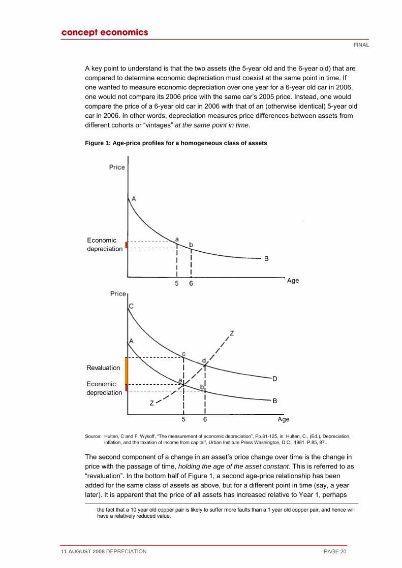
A change in the price of an asset between two points in time can be decomposed into two components. The first component is the decline in price from aging holding time constant. This is what is referred to as economic depreciation and is shown in the top half of Figure 1. The top graph in Figure 1 plots the age-price relationship of a group of otherwise identical assets of different ages at one point in time, so that the value of a 5-year old asset is represented by point a on the curve, and the value of a 6-year old asset by point b. Economic depreciation for the 5-year old asset as it ages to a 6-year old asset is the

37

age-price curve for

its useful life

ses, the efficiency of the asset is reduced as it ages (say, ntenance or

h further causes the age-price curve to slope downwards.38

difference on the vertical (price) axis between a and b (the thick red line).

With few exceptions, and unless the asset has an infinite useful life, the a given class of assets is always downward sloping, for two reasons:

• Any asset that has aged by a year has fewer “productive” years left in during which it can generate rentals; and

• Additionally, in most cabecause it is more prone to break-downs, or because it requires more maifuel), whic

f production (say, t life are directly linked

n is not a strict price taker, but where demand for the firm’s output – and how demand evolves over time – varies in response to the firm’s pricing decisions. In this case, the depreciation profile determines the price at which the asset’s output is sold, which in turn determines demand and therefore asset value and asset life. I return to this point in the context of depreciation in a regulated environment in Section 3.3 below.

35 In this (inter-temporal) formulation, dt = vt – vt+1, where vt is the value of the asset at the start of period t. 36 The following discussion draws on Wykoff, Frank C., “Obsolescence in Economic Depreciation from the Point of

View of the Revaluation Term”, February 28, 2003. 37 The rate of depreciation – the speed at which an asset’s value declines – is the elasticity of the price (AB) curve

between a and b (that is, the percentage decline in asset price between these two points). 38 Of course, an asset may experience favourable or adverse cost shocks as it ages: it may become obsolete, or

conversely, new uses for the asset may increase its value. For instance, it might be argued that the development of DSL technology increased the economic value of copper pair networks. But that in no way alters

34 Here operating costs are broadly defined to include ongoing costs arising in the course olabour and materials), but also repairs and overhauls. The fact that asset value and assecreates a circularity in a world where the firm in questio

FINAL


A key point to understand is that the two assets (the 5-year old and thecompared to determine economic depreciation must coexist at the same po

6-year old) that are int in time. If

one would not compare its 2006 price with the same car’s 2005 price. Instead, one would ntical) 5-year old en assets from

one wanted to measure economic depreciation over one year for a 6-year old car in 2006,

compare the price of a 6-year old car in 2006 with that of an (otherwise idecar in 2006. In other words, depreciation measures price differences betwedifferent cohorts or “vintages” at the same point in time.

Figure 1: Age-price profiles for a homogeneous class of assets

Economic depreciation

Economic depreciation

Revaluation

., (Ed.), Depreciation,

tion, and the taxation of income from capital”, Urban Institute Press Washington, D.C., 1981. P.85, 87..

The second component of a change in an asset’s price change over time is the change in price with the passage of time, holding the age of the asset constant. This is referred to as “revaluation”. In the bottom half of Figure 1, a second age-price relationship has been added for the same class of assets as above, but for a different point in time (say, a year later). It is apparent that the price of all assets has increased relative to Year 1, perhaps

Source: Hulten, C and F. Wykoff, “The measurement of economic depreciation”, Pp.81-125, in: Hulten, Cinfla

the fact that a 10 year old copper pair is likely to suffer more faults than a 1 year old copper pair, and hence will have a relatively reduced value.

FINAL


because of general inflation or some price effect that is specific to the assetthe price of a 5-year old asset is c and the price of a 6-year old asset is asset with a price of a in Year 1 now has a price of d in Year 2. The

. A year later, d. A 5-year old

price change from a to

ce change

change from a

r older, its

reciation works in rticular way – the asset loses about half of its value in the first five years; thereafter its

e of the price-age curve defines the asset’s an asset of a certain vintage changes as it

r decomposed

“vintages” of the rior technology the presence of

a result of eferred to as “deterioration” or sometimes “decay”.

old Toshiba ter and a 2-year old Toshiba laptop computer in 2006 can be separated into

y to fail; ar old Toshiba laptop

aster processor and more memory than the 2-year old Toshiba laptop. This is eigh the deterioration

cts determines an asset’s particular age-price profile and therefore its depreciation profile; these can therefore be

urves in Figure 1 annot separately

ne the effects caused by aging (deterioration), passage of time (capital gains or losses), and changes in vintage (obsolescence).40 What this means in the context of Figure 1 is that the depreciation effect measured by the move from a to b combines pure depreciation with obsolescence, and that the shape of the age-price curve itself embodies this effect. For example, once one specifies two of the three terms – time,

d can now be decomposed into two components:

• A pure aging effect (economic depreciation), which corresponds to the prifrom a to b; and

• Superimposed, a pure revaluation effect, which corresponds to the price to c.

These two price changes work in opposite direction, and since the asset is a yeaprice does not increase by the full effect of the revaluation.

Figure 1 assumes that the loss in the value of the asset as a result of depa pavalue does not change that much. The shapdepreciation profile, that is, how the value of ages.

The economic depreciation of an asset as drawn in Figure 1 can be furtheinto two distinct price effects:39

• The first effect on an aging asset is caused by the introduction of new asset, such as an asset constructed in a later year that embodies supeand quality improvements. This effect on the price of an aging asset of a new vintage is referred to as “obsolescence”.

• All other effects that affect the extent to which an asset deteriorates asphysical aging are r

To take the example of a computer, the difference in the price of a 1-yearlaptop computwo effects. First, and all other things equal, the 2-year old computer is more likelthis is the deterioration component of depreciation. Second, the 1-yemay have a fthe obsolescence component of depreciation, which may far outweffect. The relative importance and magnitude of these effe

expected to vary for different types of assets.

Isolating the effect of obsolescence and that of deterioration in the price cis not possible, however. Hall’s Impossibility Theorem states that one cidentify from price data alo

39 The revaluation effect can similarly be decomposed into a time and an obsolescence effect. 40 Hall, Robert E., (1968), “Technical Change and Capital from the Point of View of the Dual.” Review of

Economics and Statistics. 35, January: pp. 35-46. Wykoff (2003), P.17.

FINAL


age, and vintage – the third is determined. A three-year-old wine in 2004 m2001 wine. A vintage 2001 wine is, by definition, obse

ust be a vintage rved at age three only in 2004.

3.1.

ected in different sset loses its value

rly on in the loses more value later

are less valuable 42

at, with a finite , the present value of an asset’s future rentals declines with advancing age. In

utput before et.

accompanied by uctive capability

down time and/or the cost of repairs has e cost of

rice changes, the values of older assets change over time as a result of technological innovations that are embodied in younger assets, but also because changes in consumer preferences may make some assets obsolete.

This distinction between the underlying causes of economic depreciation – the effects of time, physical decay, and technological obsolescence on asset values – are important, because they illuminate the circumstances in which different economic depreciation profiles are likely to arise.

3.1.3.1 The effects of aging and physical deterioration

a number of landmark papers, notably by k illuminates the precise origin and meaning of economic

ferent reasons ally, Jorgenson

there is a parallel (“duality”) between assets’ relative rentals and therefore

Statistically these effects cannot be separated from price data alone.41

3. Economic depreciation profiles

In this section I explain the economic depreciation profiles that can be expcircumstances in more detail. The depreciation profile refers to how an aover time; for instance, whether an asset’s value declines more steeply eaasset’s useful life (so that depreciation is “front loaded”) or whether itin its life (so that depreciation is “back-loaded”).

Ignoring revaluation (specific or general inflation) effects, older assetsthan newer assets for a number of reasons:

• In the first instance, the decline in an asset’s value reflects the fact thuseful lifeother words, all else equal, an older asset will generate fewer units of oretirement and hence have lower economic returns than a younger ass

• Second, the decline in an asset’s value is greater in early years if it isa loss of its productive capability or “efficiency”. Such a loss in prodarises, for instance, if the likelihood of increased, or if the quality of the service flow has degenerated, or if thoperations has increased.

• The third effect relates to obsolescence. Abstracting from general p

Hotelling’s theory of depreciation was refined inJorgenson and Hall.43 This wordepreciation, but it also makes a number of subtle distinctions between diffor why assets’ prices change so that terminology is important. Specificestablished that

41 I comment on other (hedonic) techniques for estimating the relative importance of these effects below. 42 Baldwin, John, Guy Gellatly, Marc Tanguay, and André Patry, “Estimating Depreciation Rates for the

Productivity Accounts”, Statistics Canada, September 15, 2005, Pp.6ff. Fraumeni, B.M. 1997. “The Measurement of Depreciation in the U.S. National Income and Product Accounts” Survey of Current Business. July: 7-23.

43 Hall, Robert E., (1968), “Technical Change and Capital from the Point of View of the Dual.” Review of Economics and Statistics. 35, January: pp. 35-46. Jorgenson, Dale W., (1974). “The Economic Theory of Replacement and Depreciation.” in W. Sellekraets, (ed.) Econometrics and Economic Theory. MacMillan, New York.

FINAL


value over time, and the same asset’s relative productive capability. In other words, all other things equal, a more efficient asset (say, a truck that can drive further on a litre of petrol than another) is worth more than a less efficient version of the same asset.

As an asset experiences wear and tear, its productive efficiency declines. In the neoclassical capital vintage model, the decline of the physical efficiency of an asset as it ages is measured by an index φ.44 That is, the efficiency or output of an asset of a certain age τ (or “vintage” τ) is assumed to be equivalent to some fraction “φτ” of an asset of the newest vintage 0. In other words, the efficiency index φτ expresses the productive capacity of a τ year old asset relative to that of a new asset. How an asset’s efficiency evolves as it ages is a key determinant of the asset’s depreciation profile:

• The efficiency profiles describe how the productive efficiency of an asset deteriorates over time;

• The efficiency profile then translates into a corresponding age-price profile for the asset (since an asset’s value at any point in time is just the present value of its future earnings); and

• The asset’s age-price profile defines its depreciation profile (since economic depreciation is the difference between an asset’s value at two ages).

Figure 2 illustrates this sequence for three types of assets, each with a different (physical) deterioration profile. Figure 2 plots, in the top graph, an efficiency profile for each asset, next, the age-price profile corresponding to that efficiency profile (for each asset), and in the bottom graph, a corresponding depreciation profile (for each asset).

I first consider an asset whose productive capability does not physically deteriorate as it ages. This constant efficiency pattern is known as a “one-hoss-shay” pattern; it refers to assets that retain their full efficiency until they suddenly and utterly cease to function.45 All other things equal, such an asset will, in each of the productive periods over its useful life, generate a rental that is directly proportional to its productive capacity φ.

The top part of Figure 2 plots a constant efficiency (one-hoss shay) profile over the asset’s 20-year life, where it is assumed that the asset earns $1 in each year. Assuming unchanged prices, such an asset – say, a light bulb – would generate a constant stream of output and hence revenue until the end of its life. In turn, the asset a t) income

es.46 The value is high head of it and decline nomic deprec l from this calcula the discount rate is positive (i.e. there is a positive time value of money), the one-hoss shay efficiency pattern gives rise to a back-loaded economic depreciation profile.

In all circumstances where there is some form of physical deterioration of the asset (in addition to the pure aging effect), economic depreciation profiles are front-loaded. Figure 2

’s (const npattern determines its value (the present value of its future rentals) as it ag

est at the beginning of Year 1, where it has 20 years of useful life as thereafter, slowly at first and then more rapidly in later years. Ecoiation (i.e. the annual depreciation charge) emerges as a residuation, and the bottom graph plots this. It is apparent that so long as

44 Formally, the φτ is the marginal rate of substitution in production between the τ-year-old asset and the new

asset. Hulten Wykoff (1981), P.88. 45 Light bulbs are often cited as exemplifying assets of this type. 46 These numbers have all been normalised to 1.

FINAL


repeats the same logic for an asset in which efficiency deteriorates in a strageometric manner:

• Under a straight-line efficiency profile, the productive efficiency of the aequal absolute increments until the asset is retired. All other things equthat this type of asset generates similarly decline in linear increments ouseful life. With discounting, the asset’s value declines more rapidly ithan in later years, and the depreciation charge is corresp

ight-line and a

sset declines in al, the revenues ver the asset’s

n its early years ondingly higher in earlier

ncy declines is d in earlier periods

-loaded.

years (i.e. front loaded) and less in later years.47

• Under a geometric efficiency profile the rate at which an asset’s efficieconstant over the asset’s life. Revenue declines are more pronounceof the asset’s service life than in later periods, and depreciation is front

47 In a regulated setting, this depreciation profile matches that described by Jaffee for a firm that earns a constant

amount of revenue from a fixed amount of capital in an environment of certainty. Bruce L. Jaffee, 1973. "Depreciation in a Simple Regulatory Model," Bell Journal of Economics, The RAND Corporation, vol. 4(1), pages 338-342, Spring.

FINAL


Figure 2: Asset efficiency, asset prices and depreciation

Efficiency profile

$0.0

$0.2

1 2 3 4 5 6 7 8 9 10 11 12 13 14 15 16 1

Time

$0.4

$0.6

$0.8

$1.0

7 18 19 20

Geometric

One hoss shay

Straight-line

Price-age profile

$0.0

$0.2

$0.4

$0.6

1 2 3 4 5 6 7 8 9 10 11 12 13 14 15 16 17

$0.8

$1.0

18 19 20

Time

Depreciation profile

$0.0

.2

$0.4

1 2 3 4 5 6 7 8 9 10 11 12 13 14 15 16 17 18 19 20

Time

Notes: All values standardised to a maximum of $1. Calculations assume interest rate of 10%, useful asset

life of 20 years. For geometric efficiency profile, σ = 0.2. These stylised relationships between asset

efficiency and depreciation assume two simplifications: 1. Service lives and efficiency patterns are

known with certainty. 2. Asset prices reflect the actualised value of its future stream of revenues

where these revenues are a linear function of the capacity of the asset. Baldwin, John, Guy Gellatly,

Marc Tanguay, and André Patry, “Estimating Depreciation Rates for the Productivity Accounts”,

$0

$0.6

$0.8

$1.0

FINAL


Statistics Canada, September 15, 2005, Pp.6ff. Fraumeni, B.M. 1997. “The Measurement of

urvey of Current Business. July:

3.1

ermining the s and therefore

s” of capital are hnology. If this new

of “new” assets over time, but the arrival of new, better vintages may also depress prices of existing “old”

, prices of new and s of service

the is referred to as

ied obsolescence as reflected in the decline in the real price of capital assets s

t). In contrast, ital asset declines

as a result of for making

shift in demand for some product will he disposal prices duct.

the efficiency d by the

perior assets becomes (negatively) capitalised into the prices of the older, ” version of an ld”) asset’s price.

d therefore depreciation) for existing assets.

Assessing the extent to which this (depressing) price effect arises is not straightforward, becomes relatively

of the used asset ced, since the older vintage asset remains as productive as it was appeared.50 Hulten, in turn, suggests that whether price shifts from

ur depends on whether quality improvements are achieved at a cost or not, so that a price reduction from obsolescence is more likely for older assets if quality

Depreciation in the U.S. National Income and Product Accounts” S

7-23. P.6.

.3.2 The effect of obsolescence

Obsolescence is another, separate factor that plays a major role in deteconomic depreciation of an asset.48 Obsolescence changes asset pricegives rise to an economic depreciation effect, because when new “vintageintroduced into the market, they often contain new “state of the art” tectechnology is superior to what exists already, it will ordinarily raise prices

vintages of capital, which do not contain the new technology. In that wayold assets are equalised when measured in efficiency unit terms (i.e. in termpotential). This decline in value of older vintages of an asset class as a result of introduction of innovations embodied in newer vintages of the asset class“embodied obsolescence”.

Emboddescribed above is caused by new technologies that render the existing capital serviceobsolete (such as motor vehicles replacing horses as a means of transpor“disembodied” obsolescence occurs when the value of the underlying capover time due to shifts in demand or other exogenous factors.49 For instance,the declining demand for cigarettes, the demand for capital equipmentcigarettes has also declined. Thus a downwardgenerally lead to a downward shift in the demand for capital assets (and tof existing assets) in the industry that produces the declining demand pro

To summarise, while the arrival of the superior competitors does not reduceof existing assets, it can reduce their prices when the cost savings realisetechnically su(now) obsolescent vintages. In other words, the fact that a newer, “betterasset becomes available in the market has a depressing effect on the (“oIn those cases, obsolescence translates into larger price declines (an

however, and opinions differ. Griliches has argued that even if an asset obsolete because new technology generates a superior one, the value should not be redubefore the new oneobsolescence occ

48 The following discussion draws on: Hulten, Charles R., and Frank C. Wykoff (1996), Issues In The

Measurement Of Economic Depreciation, Introductory Remarks, Economic Inquiry 34 (1), P.19ff. 49 This concept goes back to Matheson, Church and Pigou. Diewert, Erwin, and Frank C. Wykoff, “Depreciation,

Deterioration and Obsolescence when there is Embodied or Disembodied Technical Change”, Revised July 12, 2007. P.11.

50 Wykoff (2003).

FINAL


improvements are costless.51 Diewert and Wykoff argue that, irrespective of its origin, rapid ing capital t is analogous to

xplain asset ristics of

assets (such as memory or computing power) suggest that, at least for certain types of sult of obsolescence are profound (so that Griliches’ thesis

rs, for instance, e-hoss-shay

d once lescence was

on profile.

3.1

ic depreciation assumes away uncertainty, so that there is no doubt about future asset prices or about the length of an asset’s useful life. Baldwin et al.

t be geometric (that is, ccount.54

nown with retired after T. If

fore T than after T), the price-en the

ss shay d.

tion profile appears ofile. Hulten and

ssets eometric

ent assets in the red at different dates; some may last a year or two, others ten to fifteen years.

rience of 1/1,000 g much closer to a

s are uncertain and when merge.

anticipated obsolescence translates into real declines in the prices of existassets, and can be interpreted as an obsolescence charge on income thawear and tear depreciation or deterioration.52

More recent empirical studies using “hedonic” estimation techniques that eprices using “objective” factors such as age, as well as “qualitative” characte

assets, declines in prices as a redoes not seem to be borne out in practice). In a study of laptop computeWykoff found that even if physical deterioration of computers follows a onpattern, value declines are steep and depreciation is very much front-loadeobsolescence is taken into account.53 In other words, in this example obsosufficiently important to reverse the “standard” one-hoss-shay depreciati

.3.3 Uncertainty and groups of assets

Most research on econom

suggest that in reality most economic depreciation profiles may in facfront-loaded), if the uncertain timing of when assets are discarded is taken into aIn Baldwin et al.’s model, the time when an asset is discarded (“T”) is not kcertainty, because some assets will be retired before T and others will be T is random and skewed (so that more units are discarded beage profile resembles that of a geometric asset shown in Figure 2, even whefficiency profile of an asset is constant (i.e., when the asset has a one hoefficiency profile).55 Depreciation correspondingly becomes front-loade

It is relevant to note that a similar geometric (i.e. front-loaded) depreciato arise in practice for groups of assets with a one-hoss shay efficiency prWykoff point out that while it may be true that every single asset in a group of 1,000 adepreciates as a one-hoss-shay, the group as a whole experiences near-gdepreciation.56 This fallacy of composition arises from the fact that differgroup are retiThus the average asset (in the sense of an asset that embodies the expeeach of 1,000 assets in the group) is not one hoss shay, but somethingeometric pattern.

To summarise, the literature suggests that when useful asset livegroups of assets are considered, a front-loaded depreciation profile is likely to e

“Endogenous Growth and the Cost of Quality Change in Capital Goods”, National Bureau of

Economic Research Summer Institute Working Paper, 1995. 52 This concept goes back to Matheson, Church and Pigou. Diewert, Erwin, and Frank C. Wykoff, “Depreciation,

Deterioration and Obsolescence when there is Embodied or Disembodied Technical Change”, Revised July 12, 2007. P.12.

53 Wykoff (2003). 54 Baldwin et al (2005), P.11ff. 55 The distribution is taken to be asymmetric—skewed to the left—with more units being discarded before T than

after. 56 Hulten Wykoff (1996), P.18.

51 Hulten, Charles R.,

FINAL


3.1.

ly calculated: it s. But although

the factors that are likely to be important in determining an economic depreciation profile – ll understood,

ust be xpected useful

eciation profiles. rly for long-lived

ntals” for stinguishes

users), and implicit). The

at of the rental, hen using a

tilised assets) may be d the quasi-rental is

xpenses are paid. to use an asset for

will converge, but with ty they may not.58 The implication is that even conceptually, determining the

assets (i.e. assets for which no explicit “rental” is apparent) ning the depreciation profile of such assets is also

economic sets in second-

d deriving economic depreciation profiles from these. However, (arguably) most assets, and in particular owner-utilised and specialised assets are never traded once

e in these , described in Table 1 below, for instance, second hand markets are unlikely to

uch assets also have a remaining value, namely the remaining outcomes resulting

ake such valuations tenuous.

d in second-hand markets, there are a number of reasons for thinking that the resulting (observed) prices are not representative of the values (in terms of their future rentals) of these assets:

4. Measuring economic depreciation

As I explained above, in theory, economic depreciation need not be explicitsimply emerges as a residual from a comparison of assets of different age

the effects of aging, deterioration, and obsolescence – are reasonably wehow these different factors interact is complex. In particular, these factors mcombined with “rentals” or the assets’ expected income streams over the elife of the asset in order to, first, derive asset prices, and, second, deprThis is a formidable computational exercise and one requiring, particulaassets, projections well into an uncertain future.

An additional complication arises from the importance of future asset “redetermining asset prices and, in turn, depreciation profiles. The literature dibetween “rentals” (the return obtained by renting the asset to subsequent “quasi-rentals” (if the machine is owner-utilised and the rental is thereforequasi-rental or “user cost of capital” concept is notionally equivalent to thsince the quasi-rental is the opportunity cost that the owner must forego wcapital asset.

However, determining quasi-rentals (and therefore values of owner-uproblematic.57 Most owner-utilised capital is fixed in the short run, anan ex post residual – the amount left over from revenue after current eThe rental is instead an ex ante concept that refers to an acquired right a stipulated period of time. Under perfect foresight, the two conceptsuncertainprices of aging, owner-utilisedis difficult, and that hence determicorrespondingly challenging.

It might be thought that, irrespective of these theoretical complications,depreciation could simply be measured by observing prices of capital ashand markets an

they have been purchased. For the majority of the assets that are at issuproceedingsexist. Theoretically, sexpected returns or quasi-rentals, but in practice, uncertainty about future(including expected demand and supply conditions, technical change andobsolescence) m

Moreover, even when assets are trade

57 Hulten Wykoff (1996), P.12. 58 Even if demand fluctuations are correctly anticipated, the ex ante expected utilisation of a capital asset may

differ from its ex post utilisation, which also leads ex ante rentals and ex post quasi-rentals to diverge. See Hulten Wykoff (1996), P.12.

FINAL


• In practice, market valuations of used assets are hard to come by.59 Smarkets tend to be “thin” or non-existent for specialised (capital) assetsfirms typically regard their own worn assets as different from (and probreplicas in the market, because their history, condition and foiblesresult, in many cases, there is a perceived “adverse selection” pfor second hand equipment, especially for specialised assets, which

econd-hand . Additionally, ably better than)

are known. As a roblem in the market

limits the “depth” of that market and distorts price formation (as it results in a gap between bid and ask

ce sampling s arises because ve survived long

of 15-year old cars sents the value of cars that have survived 15 years – many other cars of this

f the various ciation profiles

rt. It is nonetheless ndertaken for the

point to a pattern r of asset classes. aches to

inery and equipment preciation are

ken by Statistics Canada most

ing plants and

To summarise the previous discussion, while conceptually appealing, determining eciation profiles in practice is fraught with difficulties. The accounting theory

ory of d how this is translated into practice, is therefore concerned with developing

est as possible, “match” accounting depreciation approaches depreciation. At least in the accounting theory literature, the objective of

accounting depreciation is fundamentally the same as for economic depreciation: to derive a measure of the cost of holding and/or using an asset over a particular accounting period.

prices).

• Even where market valuations of used assets are available, any simple priprocedure suffers from a “censored sample bias” problem.60 The biamarket prices of used assets reflect only the value of assets which haenough to be eligible for sampling. Hence the average market price reprevintage would have already been retired from service.

Correcting for these difficulties is not straightforward, and a description oempirical approaches that have been adopted to estimate economic deprefor different classes of assets would go beyond the scope of this reporelevant to observe that recent empirical studies that have been upurposes of measuring the value of the capital stock in national accountsof geometric (i.e. front-loaded) depreciation for the overwhelming numbeFor instance, Baldwin et al conclude from their survey of empirical approestimating economic depreciation that:61

The depreciation profiles generated by the econometric techniques are, on balance, accelerated, producing convex age-price curves. Declines in value early in life are apparent for many assets in the machclass, as well as for certain structures. Evidence that rates of deconstant over service life is, on balance, mixed.

Similarly, a very recent and comprehensive study undertasuggests that geometric depreciation profiles are a good approximation formanufacturing and engineering (M&E) assets, as well as for manufacturoffice buildings.62

economic deprliterature, which can be viewed as the interface between the economic thedepreciation anaccounting rules that, as bwith economic

59 Baxter (1971), P.31. 60 Hulten Wykoff (1981),. P.91. 61 Baldwin et al., 2003. P. 53. 62 Patry, André, Statistics Canada, “”Economic Depreciation and Retirement of Canadian Assets: A

Comprehensive Empirical Study”, Catalogue no. 15-549-XIE, September 2007.

FINAL


3.2. ACCOUNTING DEPRECIATION

Broadly speaking, what I refer to as the “accounting” approach to depreciatiothe initial purchase price of an asset as its value, and to adopt accounting “rules”

n is to accept for “writing

down” that asset value over time. That is, the accounting rule determines how much value an be in each

eciation then between “time-

sponding to the causes that may bring an asset’s life to an

ne in value of t the asset valuation concept that is

eaking, the traditional accounting se price of an asset as the asset’s “value”,

over the life of

d considerably mined the notion t values. The

t financial formation contained therein serve a wide variety of users and uses.64

ntained in accounts should inform the future decisions that account users would make, less emphasis was placed on historical cost as a basis for valuing assets

ition over time), alues or future

h to depreciation nts and its ctive (in the

les should arrive at a similar figure), but may be meaningless as far as capturing the actual value or opportunity cost of an asset is concerned. In turn, current values, or “economic” present values obtained by discounting prospective receipts may be more informative about the opportunity cost or future

ify and less

the objectivity or reliability of information presented in accounts prepared on the basis of forward-looking valuation concepts are compounded in a world characterised by

asset has lost from one period to the next, and therefore what depreciation shouldaccounting period to account for that value loss. Accounting methods of deprconsider how many units of output an asset can still deliver, and distinguishassets” and “use-assets”, correend – the passage of time or “wearing out” by use.

3.2.1. The accounting theory debate

Like the economist, the accountant considers depreciation to be the declicertain capital assets between two accounting dates, buused differs from that used by economists. Broadly spapproach to depreciation takes the original purchaand requires that value (less the asset’s scrap value, if any) to be distributedthe asset, in accounting terminology, “in a systematic and rational manner.”63

Traditional accounting and its approach to measuring depreciation has evolveover the years, particularly in the 1970s and 80s, where high inflation underthat historical prices paid for assets accurately reflected contemporary assestarting point for the theoretical accounting literature from that period was thaaccounts and the inSince the information co

(other than as an element in reconciling changes in the owners’ financial posand the focus turned instead to asset values that reflected current market vearnings prospects.

But this changing focus on something more akin to an “economic” approacled to a conflict between the objectivity of the information presented in accourelevance. Historical cost data are more easily verified and are relatively objesense that two independent accountants applying the same ru

income stream associated with an asset65, but are clearly less easy to verobjective.

Problems with

63 F. K. Wright, Towards a General Theory of Depreciation, Journal of Accounting Research, Vol. 2, No. 1 (Spring,

1964), pp. 81. 64 Whittington, (1997), P.24ff. 65 At least for assets traded in secondary markets. Moreover, note that if the services provided by an asset are

regulated (in the sense of having regulated prices), there are circularity issues in basing asset valuation on expected income.

FINAL


uncertainty.66 Uncertainty implies that ex post income and value outcomes do not necessarily equal ex ante expectations, and that the present economic value of an asset cannot be established objectively in the absence of perfect and complete forward markets. In other words, there is no objective way of determining the current value of a machine that might generate one set of earnings in one set of economic circumstances (or “state of the world”), and another set of earnings in another set of circumstances.67 A further complication with user-orientated accounts is that there are a variety of users and uses, each of which might have different information requirements. To summarise, “any attempt to report the ‘true’ value of the firm’s assets or its profit for the period will encounter the problem of uncertainty, and a single choice from among the variety of measures available is unlikely to meet the needs of all potential users”.68 It is probably fair to say that, overall, and although much effort was expended on developing new, more “realistic” (accounting) valuation concepts, none (with the possible and rather limited exception of top-down current cost valuation approaches that are described below) have gained general acceptance.

A balanced assessment of accounting depreciation would then acknowledge that in an “imperfect” world, deriving depreciation on the basis of the (forward-looking) economic valuations would almost certainly be impossibly costly to undertake and would also be unacceptably subjective. Nonetheless, and as a result of the debate about asset values, more attention has been paid to developing accounts that provide important stakeholders with more meaningful measures of profits and asset valuations, and therefore also of depreciation.

3.2.2. Accounting depreciation profiles

In order to define particular depreciation profiles over time, accounting depreciation relies on (mechanical) depreciation profiles that are thought to appropriately reflect deterioration patterns of different types of assets.69 These accounting depreciation profiles allocate an asset’s price (either in historical or in current cost terms) over its useful life to arrive at the asset’s net book value.

The starting point for an accounting depreciation profile is to consider how many units of output an asset can still deliver. Here the distinction is made between “time-assets” and “use-assets”, corresponding to the causes that may bring an asset’s life to an end – the passage of time or “wearing out” by use.70 Use-assets are those where there is a cause-and-effect link between an asset’s use and the point in time at which it has to be replaced, say, an aircraft

assets include assets whose life will be ended by obsolescence; other time limits arise from patents,

engine that must be replaced after it has run for a thousand hours. Time

66 Whittington, (1997), Pp.26-27. 67 Moreover, in such a world of incomplete markets, the traditional (Hicksian) economic concept of “income” may

not have an unambiguous meaning, so that there is no ready ‘anchor’ for determining an approach to depreciation. See Beaver W. H. (1997, 3rd ed.) Financial Reporting: An Accounting Revolution, Prentice Hall, Inglewood N.J.

68 Whittington, (1997), P.27. 69 Baxter (1971) provides an excellent overview of how economic depreciation concepts are translated into

accounting depreciation approaches. 70 Baxter (1971), P.61ff.

FINAL


contracts, time-limited franchises or general physical deterioration from causes other thanuse.

rofile are then the cost depends on

With time-time and the

approach of the asset’s removal from service. In other words, use-depreciation is a function tion of “time-units”

ermined there are that I will not go into

the initial price tricity), and the cost of

ut how such certain types of revenues) are reflected in depreciation patterns.

logy is appropriate cash flow and

. Recurring outlays for an asset may increase, decrease or stay constant, and may include one or more regular

activity pattern of use-assets may increase, decrease, or stay whole cost of

ears affects a firm’s costs

calculating useful life, first,

d third, the depreciated alue, and it does so for the following depreciation methodologies:

al percentage o-period, the riod-to-period –

t the diminishing net value of an asset is written down by a constant percentage in each accounting

d, so that the charges t would lead to such

increasing repair

71

What is relevant for the purposes of deriving an accounting depreciation ppatterns of the relevant activity.72 With use-assets, a figure for depreciationthe extent of usage; it is high in years of high use, and low in years of low use. assets, use costs nothing: the depreciation charge measures the passage of

of “service-units” such as miles run, whereas time-depreciation is a funcsuch as years.

Even when asset valuation and depreciation methodology have been detmany additional complications that arise from an accounting perspective here. Often a wide range of outlays are connected with an asset, including paid for it, the cost of operating it (such as operatives’ wages and elecnormal and abnormal repairs.73 There are then a number of questions abooutlays (but also

What is clear however, is that whether a particular depreciation methodofor a particular asset depends on whether it fits in with the asset’s pattern of activity.74 These patterns vary greatly for different kinds of assets

overhauls. Likewise, theconstant. Even though all accounting depreciation methods aim to write off thean asset by the end of its life, the spread of this burden between yand profits, particularly where depreciation is a big part of a firm’s costs.

Figure 3 charts the most commonly used traditional accounting methods fordepreciation for time assets. Figure 3 illustrates, for each year of an asset’s how depreciation is calculated, second, cumulative depreciation, anasset v

• SLD assumes that the value of the asset declines by a constant and equin all accounting periods. Although the dollar loss is equal from period-trate of depreciation – that is, the percent change in asset value from peincreases progressively over the course of an asset’s service life.

• Fixed percentage of the declining balance depreciation assumes tha

period. This is an accelerated (front-loaded) depreciation methohave a high-low pattern and the value curve sags. The factors thaa depreciation profile are rapid early deterioration, obsolescence, andcosts.

71 In practice, of course, assets may combine both time and use aspects of depreciation, so that the distinction is

not necessarily clear. 72 Baxter (1971), P.66ff. 73 Baxter (1971), 41ff. 74 Baxter (1971), P.69ff.

FINAL


• Sum-of-years’-digits depreciation assumes that the value of the asset ddecreasing fraction in each accounting period. Sum-of-years'-digits depin a more accelerated write-off than SLD, but less than the declining-bUnder this method annual depreciation is determined by multiplyinamount by a schedule of fractions.

eclines by a reciation results

alance method. g the depreciable

t in all years), nt-loaded forms of sset’s life. All of

e “service-unit” method its an asset can

3.3

d to the economic circumstances, this leads

ers of a e essence of the

ariance Proposition es, and once more

are adopted about the context in which the regulated firm operates, the

of “forward- its economic

general, be or has determined future

wed revenues), ce

aths price path

is such that a forward-looking appraisal of the asset (that is, the present value of its future earnings) at

al, it can be

With the exception of SLD (which provides for a constant depreciation amounthe depreciation methods pictured in Figure 3 represent “accelerated” or frodepreciation, since dollar depreciation is higher in the earlier periods of an athe methods illustrated here also relate to time assets. In contrast, thfor use-assets begins with an assumption about the number of service unyield over its lifetime, and simply allocates depreciation accordingly.

. DEPRECIATION IN A REGULATORY SETTING

In a regulatory setting, depreciation profiles are no longer immediately linkecharacteristics of the capital assets in question. In certain restrictiveto a circularity between regulated prices and asset values, so that shareholdregulated firms are indifferent which depreciation profile is adopted. This is th“Invariance Proposition”. However, even in circumstances where the Invholds, different depreciation profiles have different social welfare propertirealistic assumptionsproposition breaks down.

3.3.1. The Invariance Proposition

In a regulatory setting where regulated prices are calculated on the basislooking” costs, the link between an asset’s future earnings, its value anddepreciation profile is a circular one, and economic depreciation cannot, ininterpreted as an opportunity cost.75 That is, once the regulatprices that may be charged for the regulated service (and therefore alloasset values and therefore depreciation profiles over time follow. In this sense, the choion the part of the regulator of one of any number of future regulated price pcorresponds to a choice of a depreciation profile, since each regulated corresponds implicitly to an asset value. As long as the depreciation profile

any point in time yields an internal rate of return equal to the cost of capitdescribed as economic depreciation.76

75 Salinger, Michael Al, “Regulating Prices to Equal Forward-Looking Costs: Cost-Based Prices or Price-Based

Costs?” Journal of Regulatory Economics; 14: 149-163 (1998). 76 This concept of depreciation is referred to as “Hotelling depreciation”: the allocation of the cost of a durable

asset over its life so that the expected profit in each period divided by the expected net asset value equals the internal rate of return.


FINAL

Figure 3: Common accounting depreciation methods

Depreciation

$80

$120

$160

$200

$0

$40

1 2 3 4 5 6 7 8 9 10 11 12 13 14 15 16 17 18 19 20

Time

Straight-line

Declining balance

Sum of digits

Cumulative depreciation

$1,000

$01 2 3 4 5 6 7 8 9 10 11 12 13 14 15 16 17 18 19 20

Time

$200

$400

$600

$800

Asset value

$1,000

$600

$400

$200

$0

$800

1 2 3 4 5 6 7 8 9 10 11 12 13 14 15 16 17 18 19 20

Time

Notes: Figures assume an initial outlay of $1,000, an asset life of 20 years, and a scrap value of $50.

PAGE 34

FINAL


It could be argued that, as long as a regulated firm’s shareholders are fully compensated for ecise form of ern them too where a regulated ce Proposition

preciated original then the NPV of all

r any method of computing depreciation (so that shareholders neither profits).

, the choice of arge to recover the regulation adjusts

ir discounted ation schedules always equal the differences in these assets’

alue of an asset as long as the sum of depreciation precisely recovers

the cost of the original investment, shareholders are indifferent between depreciation set will equal its

However, as I explain in the next sections, the Invariance Proposition does not consider nment under

is not generally the rent depreciation profiles.

be assured that they will recoup e that all

rofiles are equally socially desirable.79 An inappropriate choice of depreciation s no relation to the oreover, and even in n that shareholders

optimal

, the choice of depreciation policy is equivalent to selecting one of many intertemporal patterns of regulated prices, all of which will yield a revenue stream

ach of which can oice of depreciation policy may then be

defined as the selection of one of these intertemporal patterns of prices, which will yield one of the revenue streams adequate to compensate investors.

the cost of the asset the firm invests in (including the cost of capital), the prdepreciation (that is, which depreciation profile is adopted) should not concmuch. Schmalensee’s “Invariance Proposition” defines the circumstances firm77 is indifferent between alternative depreciation profiles.78 The Invarianstates that if a regulated firm is allowed to earn its cost of capital on the decost of its investments, and if actual revenues equal allowed revenues, investments is zero fomake a net loss nor earn extra

The Invariance Proposition arises because under rate-of-return regulationdepreciation profile determines the stream of prices that the firm may chcost of the investment in the asset. The proposition implies that “perfect” prices and therefore allowed revenues so that asset prices always equal thefuture earnings, and depreciprices. Depreciation then becomes a balancing item for the economic vbetween two accounting periods, and

schedules: the internal rate of return on the cash flows of any particular asallowed rate of return.

broader, social welfare objectives, and only holds in a highly stylised envirowhich cost recovery by the regulated firm is guaranteed. In other words, itcase that a regulated firm is indifferent between diffe

3.3.2. Optimal depreciation policy

Even in a “perfect” regulatory world where shareholders canthe value of their investment and a corresponding return, it is not the casdepreciation ppolicy can lead to an intertemporal pattern of regulated prices that bearcorresponding intertemporal pattern of the opportunity cost of capital. Mthe absence of competition, the choice of a depreciation profile may meado not recover the cost of their investment, and more generally lead to subinvestment.

In the Schmalensee world

adequate to compensate investors. Given an asset’s costs there may be many alternative streams of regulated prices (containing a depreciation component), edeliver investors their required returns. The ch

77 Of course, references to a “regulated firm” having preferences in this context refer to its shareholders. 78 Schmalensee, Richard, 1989. "An Expository Note on Depreciation and Profitability under Rate-of-Return

Regulation," Journal of Regulatory Economics, Springer, vol. 1(3), pages 293-98, September. 79 William J. Baumol, 1971. "Optimal Depreciation Policy: Pricing the Products of Durable Assets," Bell Journal of

Economics, vol. 2(2), pages 638-656, Autumn.


FINAL

PAGE 36

nother. In efficient use of ther an

ther or not an e time pattern of

tion profile) may me asset may e, some

comes an eir investment.

files that permit the supply and capital assets and

m the point of investors, an initial investment decision estment and a rate of

investment f consumers of the

ing to pay the ition, wasteful. ith a fixed life and

the one-hoss shay efficiency profile described in Section 3.1.3. If general price levels are is optimal:

, regulated prices should reflect only short ent; while

ld be charged a t. In other words, d, and any

depreciation

ad pricing problem. In “off-peak” years se of the asset by nce demand

mand with supply and ol’s scenario

asset. If it is assumed that the asset in que at it becomes

optimal regulated price must contain a payment for the marginal cost of this deterioration, which is essentially a payment for future output losses.

However, one depreciation profile may then be better than another if one set of intertemporal (regulated) prices results in a better allocation of resources than athis sense, an optimal depreciation profile is one that results in the most resources. At the same time, the depreciation profile becomes key to wheinvestment is efficient in the first place. Unless demand is fixed, wheinvestment in a particular asset will turn out to be profitable depends on thprices selected.80 One pattern of prices (corresponding to one depreciamean that the investment is profitable, while another may mean that the sanot be worth its cost. In other words, if consumers are at all price responsivdepreciation profiles will produce regulated prices at which the asset beuneconomic investment and shareholders do not recover the cost of th

Baumol develops a simple investment model to identify depreciation proregulated firm to recover the cost of an investment in a way that equates demand, and results in an optimal intertemporal pattern of investment in the use of those capital assets.81 Frowill only be worthwhile if they are returned the cost of the original invreturn on that investment. Furthermore, from the point of view of society anshould be undertaken only if it is expected to offer at least this return. Igoods or services to be produced with the aid of the investment are unwillopportunity cost of the asset in question, then the investment is, by definBaumol examines the case of an (incremental) investment in an asset w

constant and there is no uncertainty, the following depreciation policy

• In years in which the asset is not fully usedrun marginal costs and should not contain a depreciation compon

• In those years in which the asset is used to capacity, consumers shouprice which just induces them to purchase the output of the investmenregulated prices should be set with reference to the elasticity of demandifference between regulated prices and marginal costs makes up thepayment for that period.

In effect, Baumol describes an intertemporal peak-lo(when the asset is not fully used) it is always desirable to increase the ulowering regulated prices, provided that marginal costs are recovered. Oreaches capacity, price becomes the rationing device to equalise dethe regulated firm recovers (some or all of) the cost of the investment. Baumcan also be expanded to take into account the physical deterioration of an

stion physically deteriorates over time (so thless productive), the

80 In other words, there is a duality relationship between the optimal investment program and the optimal pricing

(depreciation) policy. William J. Baumol, 1971. "Optimal Depreciation Policy: Pricing the Products of Durable Assets," Bell Journal of Economics, vol. 2(2), pages 638-656, Autumn.

81 William J. Baumol, 1971. "Optimal Depreciation Policy: Pricing the Products of Durable Assets," Bell Journal of Economics, vol. 2(2), pages 638-656, Autumn. P.642ff.

FINAL


Baumol’s results relate to an investment that is perfectly divisible, so that apricing rule will recover the cost of the investment. If this is not the case, a

marginal cost revenue

constraint has to be added to the optimisation problem to ensure that sufficient depreciation is collected to recover the original cost of the investment, which will in turn determine deviations of prices from marginal costs. In this sense, Baumol’s approach reverts to the rules for maximising welfare (or rather, minimising efficiency losses) subject to a revenue constraint, and therefore the “Ramsey-Boiteux” theorems for optimal departures from marginal cost pricing.82 In other words, to recover the cost of the asset, regulated prices should be set in inverse proportion to the price sensitivity of consumers’ demand, so as to ensure that demand is “distorted” (that is, changed from what it otherwise would have been had all prices been set at marginal cost) as little as possible.

Baumol and Sidak comment in more detail on cost recovery for “lumpy” investment in regulated industries, such as the electricity industry.83 Here it is the case that timely investment is typically undertaken in step increments, so that there will always be some “excess” capacity in the system. In that context, Baumol and Sidak argue that in recovering the cost of a lumpy plant over its lifetime, the payments should be timed as they are in any competitive market. Thus, the sum of the revenues over the lifetime of the investment should be sufficient to cover all costs, including replacement of the investment (as well as the cost of the capital tied up in the investment during its lifetime). The timing of these revenues, however, cannot be determined definitively by the regulator, but is ultimately affected (if not entirely determined) by the state of the market at different periods during the lifetime of the investment.

In Baumol’s analysis, the firm’s profit maximisation objective and the regulator’s social welfare objectives generally coincide. Burness and Patrick investigate a similar model of a firm that is operating under a rate of return constraint and invests in a single asset.84 In this case, the firm’s objective may diverge from that of the regulator, depending on the relationship between the allowed rate of return and its cost of capital: if the allowed rate of return exceeds the regulated firm’s cost of capital, the firm will prefer a back-loaded depreciation profile (since it can increase its profits by depreciating the asset as slowly as possible); the firm will prefer a front-loaded depreciation profile if the allowed rate of return is less than its cost of capital. In that sense, a preference for a front-loaded profile will tend to be stronger, the greater the probability investors attach to the risk that the regulator will set the allowed rate of return below the cost of capital.

3.3.3. Competition and technical progress

Schmalensee’s model (and the regulatory literature of depreciation in general) assumes ex ante capital maintenance, that is, the regulatory bargain provides for full cost recovery of any investment. Even if this assumption is maintained, once competition and technological

82 Frank Ramsey, “A Contribution to the Theory of Taxation, Economic Journal, Vol. XXXVII (March 1927), and M.

Boiteux, “Sur la gestion de Monopoles Publics astreints à l’équilibre budgétaire,” Econometrica, Vol. 24 (April 1956). Baumol paper is itself an extension of: S. C. Littlechild, “Marginal-Cost Pricing with Joint Costs”, The Economic Journal, Vol. 80, No. 318 (Jun., 1970), pp. 323-335; and Ralph Turvey, “Marginal Cost”, The Economic Journal, Vol. 79, No. 314 (Jun., 1969), pp. 282-299.

83 William J. Baumol & J. Gregory Sidak, The Pig in the Python: Is Lumpy Capacity Investment Used and Useful?, 23 Energy Law Journal. 383, 390 (2002).

84 Burness, H Stuart & Patrick, Robert H, 1992. "Optimal Depreciation, Payments to Capital, and Natural Monopoly Regulation," Journal of Regulatory Economics, Springer, vol. 4(1), pages 35-50, March.

FINAL


change are introduced into Schmalensee’s model, the Invariance Proposholds.

ition no longer

logical progress of its

restricts the price nues generated

at then the ability of the regulated firm to recover n: if there is iation is essential if plies that the same

ds more cheaply than in current periods, so that, in the e cheaply than

stance, if regulated the asset’s life), this effectively eliminates

outlays, so that the regulated st of historical

is technological requires that

depreciation is set optimally.

3.3.4

rd-looking cost etition and

y practice, the or

elimina

• De sses could re

• hnologies; and

• Al it is no longer in

rate recovers re price trends, price

st of new equipment, discount rates, and future asset utilisations, as well as asset lives and demand growth. Specifically Salinger notes that:

Crew and Kleindorfer consider a regulated firm that is confronted with techno(so that existing assets become technically obsolescent) and competition in some

85product lines. Under these circumstances, the threat of competitive entry of the output produced by an asset and therefore the timing of regulated reveby the asset. Crew and Kleindorfer show thits investment is affected both under rate of return and price cap regulatiocompetition and technological progress, accelerated (front-loaded) deprecthe regulated firm is to remain viable. Technological change essentially imoutput can be produced in future perioabsence of barriers to entry, new entrants can produce the same output morincumbents.

If, in addition, accelerated depreciation is delayed by the regulator (for inprices do not permit for cost recovery early on in any “window of opportunity” for the regulated firm to recover its investmentpast mistakes can no longer be rectified. Once costs have fallen sufficiently, firm must charge a “competitive” price, so that it can no longer recover the coinvestment. This window of opportunity becomes shorter, the more rapidchange and the stronger is competition facing the firm, and therefore

. Uncertainty and regulatory error

Salinger considers in more detail the challenges to implementing a forwastandard in an industry such as telecommunications that is exposed to comptechnical change.86 Salinger notes that, in contrast to “traditional” regulatorthreat of competition to (some aspects of) regulated firms’ activities substantially weakens

tes the ability of regulators to:

lay the introduction of new technology (so that the regulated businecover the cost of old assets);

sulate regulated businesses from competition from old and new tecIn

low a regulated business to recover part of the cost of an asset afteruse.

Implementing a forward-looking cost model whereby the implied depreciationthe cost of the initial investment requires forecasts, inter alia, of futuchanges of co

85 Crew, Michael A & Kleindorfer, Paul R, 1992. "Economic Depreciation and the Regulated Firm under

Competition and Technological Change," Journal of Regulatory Economics, Springer, vol. 4(1), pages 51-61, March.

86 Salinger, Michael Al, “Regulating Prices to Equal Forward-Looking Costs: Cost-Based Prices or Price-Based Costs?” Journal of Regulatory Economics; 14: 149-163 (1998).

FINAL


• Th the as depreciation when a firm m ice; and

• Uncerta creases forward-looking costs, potentially

Invariance lop a

er practical e include differences

prices come

3.4

economic and files, the

ecific

usual instances re and when

reciation profile over olution of the

nd sampling asset omic depreciation is fraught with difficulties since markets for used

election problems, pling bias. epreciation hold even for

“complete” locate an

ccounting eek to mimic economic

l complexities that are inherent in economic depreciation approaches.

The regulatory depreciation literature focuses specifically on how the capital assets of regulated firms should be depreciated. In an “ideal” system of regulation in which “regulators are assumed to follow basic textbooks and thus to allow the firm to recover depreciation expense .. plus the allowed rate of return on the depreciated original cost of the investment”, regulated firms are indifferent between depreciation profiles.88 Within the context of this

e possibility of competition decreases the length of time over which the cost ofset can be recovered and therefore results in “front-loaded”u unst dertake sunk investments to provide a good or serv

inty about asset lives similarly insubstantially so.

It is worth finally briefly mentioning Awerbuch, whose focus in analysing theProposition is more on uncertainty and regulatory error.87 Awerbuch does not deveformal model of the regulated firm, but nonetheless points to a number of othfactors that would also render the Invariance Proposition invalid. Thesbetween actual and allowed revenues, arising, for instance, as a result of forecasting errors, differences in timing between when the asset is installed and when regulatedinto effect, and a number of others.

. CONCLUSIONS

In this section I have described the factors that are identified in theaccounting theoretical literature as determining different depreciation prodistinction and rationale for accounting depreciation profiles, and the spconsiderations that apply for depreciation in a regulatory setting.

Economic depreciation only leads to back-loaded depreciation profile in un– namely when assets generate constant or increasing rentals into the futuobsolescence plays no role. More generally, deriving an economic deptime requires a detailed understanding of and foresight about the future evprices of the assets that must be depreciated. In practice, observing aprices to measure econassets tend to be “thin” or non-existent, and may suffer from adverse sand because those asset prices that are observed inherently reflect a samMoreover, it is important to avoid “fallacies of composition” in determining dprofiles, as the patterns that may seem justified for a single asset can fail tocollections of assets that are seemingly identical.

Instead of attempting to infer the price patterns that would be generated bymarkets for used assets, accounting depreciation instead relies on “rules” that alasset’s price over its useful life to arrive at the asset’s net book value in each aperiod. There is a wide range of choices of accounting profiles that sdepreciation profiles, but that avoid the conceptual and practica

87 Awerbuch, Shimon, “Depreciation and profitability under rate of return regulation”, Journal of Regulatory

Economics, Issue Volume 4, Number 1 / March, 1992, Pages 63-70. 88 Schmalensee (1989), P.294.


FINAL

PAGE 40

applied to e.

I conclude from the economic literature that I have reviewed that there are at least two ould not be the case that Telstra (and indeed, society) would be indifferent

Invariance from an economic

welfare perspective: an arbitrary depreciation profile can lead to a pattern of regulated prices opportunity cost of capital. Having said that, in

periods for the ds to be complex. In those circumstances, “Ramsey” pricing

o are the least price tend to be difficult

t, and the results can be highly sensitive to the assumptions.

Second, and irrespective of these general welfare implications, the Invariance Proposition breaks down when financial capital maintenance is not assured. The literature points to a range of circumstances when this is the case, most importantly if the regulated firm is exposed to competition and technological change that reduce asset prices. In particular these last two factors, which potentially threaten the ability of the regulated firm to recover the cost of its investment would reasonably lead the firm to adopt front-loaded depreciation profiles. The preference for such front-loaded depreciation profiles would be accentuated by any risk that the regulator would act in a time-inconsistent manner, as that risk reduces the credibility of promises by the regulator to ensure future recovery of amounts deferred to future periods.

“Invariance Proposition”, questions about whether or not the depreciation profileTelstra’s ULLS assets is “reasonable” should therefore (theoretically) not aris

reasons why it wbetween different depreciation profiles for its ULLS assets.

First, even if financial capital maintenance is assured (as is assumed by theProposition), different depreciation schedules are not equally desirable

over time that bears little resemblance to thethe presence of fixed and sunk capital assets, attributing costs to different timepurpose of recovering costs tenprinciples are applied, which place the bulk of charges on customers whsensitive. Ramsey pricing, however, involves numerous assumptions thatto tes

FINAL


4. WHETHER THE DEPRECIATION APPROACHES ADOPTED BY TELSTRA AND THE ACCC ARE “REASONABLE”

In the previous sections of this report I described the economic framework I have adopted for assessing whether a particular approach to depreciation is “reasonable”. In my opinion, any depreciation approach applied to a regulated firm must first and foremost ensure that the firm recovers efficiently incurred costs.

I have reviewed the relevant economic and theoretical accounting literature on depreciation, including the research on depreciation in a regulatory setting. The general conclusions I draw from that literature in the context of this report are that:

• Economic depreciation profiles, while economically “correct”, are complex to derive, particularly in an uncertain world. They also cannot be observed easily, and this is in particular the case for certain types of fixed and sunk assets for which there are no second-hand markets as is the case here.

• While it may be the case that in some stylised circumstances any depreciation profile – provided it meets the financial capital maintenance criterion – can be applied in a regulatory setting, in practice that is not the case. More specifically, when the regulated firm’s future revenues are at risk, for instance, because of the risk of technological bypass, depreciation profiles should be front-loaded.

corresponding interpretation of the statutory criterion that must pproach to ast been applied

above – that of ex regulated firm – is consistent with the

xtent that the ACCC’s tilted annuity approach implies that capital is not maintained, I consider that this approach is not

4.1

achieve the Act”).

The Australian Competition and Consumer Commission must not accept an undertaking e undertaking at are relevant

er particular terms and conditions of an access

(a) whether the terms and conditions promote the long-term interests of end users of carriage services or of services supplied by means of carriage services;

(b) the legitimate business interests of the carrier or carriage service provider concerned, and the carrier’s or provider’s investment in facilities used to supply the declared service concerned;

In this section I describe mybe applied to the terms and conditions of Telstra’s undertaking, Telstra’s adepreciation, and the (alternative) depreciation approach that has in the pby the ACCC. In my opinion, the central policy objective that I describedante (expectational) capital maintenance for a statutory criterion. To the einvestors’ financial reasonable.

. THE STATUTORY CRITERION

I have been asked to consider whether the ACCC’s depreciation approachstated objectives of Part XIC of the Trade Practices Act 1974 (“the

unless it is satisfied that, inter alia, the terms and conditions specified in thare reasonable (s 152BV(2)(d)). Section 152AH(1) sets out the matters th(without limitation) to determining whethundertaking are reasonable:

FINAL


(c) the interests of persons who have rights to use the declared service

(d) the direct costs of providing access to the declared service concerned;

(e) the operational and technical requirements necessary for the safe and reliable operation of a carriage service, a telecommunications network or a facility;

(f) the economically efficient operation of a carriage service, a telecommunications network or a facility.”

Section 152AB(2) furthermore provides that in determining whether the terms and conditions of an undertaking promote the long-term interests of end users of carriage services or services supplied by means of carriage services (“listed services”), regard must be had to the extent to which the terms and conditions are likely to ach g

d services;

n to carriage

ctive of encouraging the economically efficient use of, and the

; and

(ii) any other infrastructure by which listed services are, or are likely

of expectational sent context I

rinciples. asonable” to imply

is consistent with a sustainable regulatory bargain, and specifically that is consistent with financial capital maintenance and time consistency objectives.

The essence of the ACCC’s chosen approach to modelling costs – the TSLRIC approach – is to evaluate the costs that would be incurred were an entirely new, hypothetically fully efficient, network constructed. That evaluation will result in a quantum of capital costs (the costs of the assets required for the network) and of O&M costs. In principle, the return of the sum of these capital costs in the form of depreciation is then “promised” to the investor,

argain” required for the investment to take place. Given that promise, an investor starting from scratch in a hypothetical, fully contestable, market would be willing to enter into a long-term contract with the regulator for the supply of that network and its services. A depreciation regime that meets that “promise” is time consistent and “reasonable”. In contrast, varying the depreciation regime once it is made – in a way which reneges on the return of the promised amount – is the essence of time inconsistency.

concerned;

ieve the followin(limited) objectives:

(c) the objective of promoting competition in markets for liste

(d) the objective of achieving any to any connectivity in relatioservices that involve communication between end users;

(e) the objeeconomically efficient investment in:

(i) the infrastructure by which listed services are supplied

to become, capable of being supplied.”

In Section 2 of this report I have referred to the central economic objectivecapital maintenance and time-consistency of regulatory policies. In the preinterpret the term “reasonable” as being consistent with general economic pSpecifically, and from an economic perspective, I interpret the term “rean approach that

and it is that “promise” that constitutes the “fair b

FINAL


In my opinion, this interpretation is consistent with the formulation of Section 152AH(1) and Section 152AB(2).

From an economic perspective, the requirement for expectational capital maintenance is reflected in clauses (a) (b), and (c) of Section 152AH(1), which refer to the long-term interests of end users, the legitimate business interests of the carrier or carriage service provider, and the interests of persons who have rights to use the relevant service. Quite simply, and as I have explained in Section 2, any approach to depreciation that does not assure cost recovery of efficiently incurred investment is not sustainable in the sense that such an approach would fail to attract the investment required to maintain and augment an infrastructure network. Such an outcome would serve neither the interests of the carrier (or rather its shareholders), nor those of end users or any other party with a right to use the relevant service.

In my ulated in

cover the and for the

service (since prices would have been set “too low”), and thereby encourage additional utput and competition predicated on prices that

e), to the extent that depreciation failed to recover the costs of subsidy with no

nsistent with the ces that failed to

ncentive of ers to enter the market with lower cost facilities.

Below I first describe the approach that Telstra has adopted for determining depreciation this has been

eploying a current pproach.89 This

ital. st factors” for each year of the assets’

lives, which comprise depreciation and the opportunity cost of capital:

• Depreciation is calculated using the SLD method;

• The opportunity cost of capital is calculated by applying the vanilla post-tax WACC to the written down value of the asset.

opinion, such an interpretation is also consistent with the objectives formSection 152AB(2). Specifically:

• In relation to clause (c), although a depreciation approach that fails to reprovider’s investment costs may, in the short term, generate additional dem

entry, over the longer term, patterns of oare not viable for the access provider are not sustainable.

• In relation to clause (efficient investment, prices charged to consumers would incorporate a apparent and offsetting social benefit and would therefore not be coeconomically efficient use of the asset. Additionally, inefficiently low prirecover the full costs of an investment would reduce the ability and icompeting service provid

4.2. DEPRECIATION IN THE TEA MODEL

for the various assets required to provide the ULLS. I then set out how modified by the ACCC.

4.2.1. Telstra approach

I am instructed that Telstra’s TEA Model calculates the capital cost of dbest practice Customer Access Network (“CAN”) using a “building block” aapproach separately calculates depreciation and the opportunity cost of capSpecifically, the TEA Model calculates “capital co

89 Telstra, Telstra’s Efficient Access Model, Model Documentation, 3 March 2008, P.51ff.

FINAL


The capital cost factors are calculated for each asset category and vary over the assets’ l asset categories lives. The TEA Model assumes a range of asset lives for different capita

(Table 1).

Table 1: TEA Model default asset lives

Source: ACCC Discussion Paper, P.41.

Each of the annual capital cost factors, which are calculated for each year of an asset’s life, are converted into an annuity over the relevant asset’s life. The effect of this calculation is

t regulated prices

4.2.2. ACCC approach

The ACCC has and Telstra have, since its first PSTN Undertaking assessment, relied on a tilted annuity for estimating the TSLRIC of both PSTN OTA and ULLS.90

to deliver a payment stream that delivers the same NPV, but evens ouover the life of the asset. At the same time, it has the effect of converting a SLD (accounting) depreciation profile into a back-loaded depreciation profile.

90 The ACCC’s tilted annuity, TXt, is given by TXt = (1+g)t-1 ·V· (r-g) / {1-((1+g)/(1+r))N} t = 1, 2, …N, where V is the

cost of the asset, r is the rate of return, g is the tilt factor and N is the asset life. See Australian Competition and Consumer Commission, 2000, A Report on the Assessment of Telstra’s Undertaking for Domestic PSTN Originating and Terminating Access Services, July. P. 102.

FINAL


For example, in its draft decision on ULLS pricing principles and indicative prices, the applied a “tilt” to the

ach. By regulated assets) into

cost of capital ction that

ACCC states that it has used Telstra’s calculated price trends and has annuitised capital charge derived by Telstra.91 Figure 4 illustrates this approinserting a “tilt factor” (corresponding to the expected price trend for the formula used to annuitise an income stream (in this case, the sum of theand depreciation), the annuity is transformed from a “flat” function into a funslopes upward.92

Figure 4: Flat versus tilted annuity

$0

$5

$10

$15

$20io

$25

$30

$35

1 2 3 4 5 6 7 8 9 10 11 12End of year

Dep

reci

atn

Flat annuity

Tilted annuity (3% asset price trend)

Tilted annuity (6% asset price trend)

Notes: Calculations assume the initial cost of the asset to be $100, the discount rate is 15.89%, the life of

the asset is 12 years.

nt of back-loadin ng the time when

ts of historical 5 illustrates this

• A SLD profile;

• The depreciation profile implicit in a (flat) annuity;

• The depreciation profile implicit in a tilted annuity that has been constructed assuming that the price of the relevant asset increases by 3 per cent each year; and

• The depreciation profile implicit in a tilted annuity that has been constructed assuming that the price of the relevant asset increases by 6 per cent each year.

It is apparent that the effect of annuitising the capital charge is to back-load depreciation, and that this effect is more pronounced if a tilted annuity is used. If the (assumed) trend in asset

The effect of the tilted annuity approach is to superimpose a further elemeg on the depreciation profile applied to the relevant assets, postponi

the historical cost of these assets can be recovered.

All things equal, a delay in the time when Telstra is able to recover the cosinvestment increases commercial and regulatory risks for Telstra. Figureeffect. It compares different depreciation profiles, namely:

91 ACCC, DRAFT Unconditioned Local Loop Service Pricing Principles and Indicative Prices, April 2008. P.9. 92 Conversely, a negative tilt factor results in a downward sloping function.

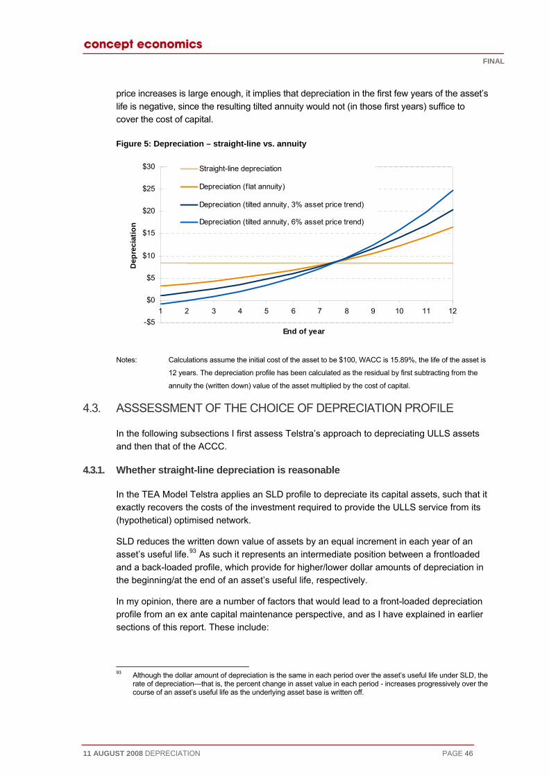
FINAL


price increases is large enough, it implies that depreciation in the first few years of the asset’s life is negative, since the resulting tilted annuity would not (in those first years) suffice to cover the cost of capital.

Figure 5: Depreciation – straight-line vs. annuity

-$5

$0

$5

1 2 3 4 5 6 7 8 9 10

De $10

$15

$20

$25

$30

11 12

prec

iatio

n

End of year

Straight-line depreciation

Depreciation (f lat annuity)

Depreciation (tilted annuity, 3% asset price trend)

Depreciation (tilted annuity, 6% asset price trend)

the life of the asset is

12 years. The depreciation profile has been calculated as the residual by first subtracting from the

asset multiplied by the cost of capital.

4.3 OFILE

ULLS assets

4.3.

sets, such that it rvice from its

(hypothetical) optimised network.

ch year of an a frontloaded

preciation in

that would lead to a front-loaded depreciation profile from an ex ante capital maintenance perspective, and as I have explained in earlier sections of this report. These include:

Notes: Calculations assume the initial cost of the asset to be $100, WACC is 15.89%,

annuity the (written down) value of the

. ASSSESSMENT OF THE CHOICE OF DEPRECIATION PR

In the following subsections I first assess Telstra’s approach to depreciatingand then that of the ACCC.

1. Whether straight-line depreciation is reasonable

In the TEA Model Telstra applies an SLD profile to depreciate its capital asexactly recovers the costs of the investment required to provide the ULLS se

SLD reduces the written down value of assets by an equal increment in eaasset’s useful life.93 As such it represents an intermediate position betweenand a back-loaded profile, which provide for higher/lower dollar amounts of dethe beginning/at the end of an asset’s useful life, respectively.

In my opinion, there are a number of factors

93 Although the dollar amount of depreciation is the same in each period over the asset’s useful life under SLD, the

rate of depreciation—that is, the percent change in asset value in each period - increases progressively over the course of an asset’s useful life as the underlying asset base is written off.

FINAL


• Risks associated with regulatory discretion and error, in particular in reperiodic revaluation of Telstra’s capital base, whic

lation to the h threaten the ability of the firm to

ould tend to s network. These

ld translate into a er way, the objective of deriving, from

y opinion, not only difficult, but in all likelihood extremely contentious. Specifically, given the

rates, deriving

e useful life of

mand for the

their future efficiency .

ould reflect the d-hand markets

the SLD approach hat is both easily

es no particularly s or efficiency trends

underlying asset

s that I have ope for

Telstra is reasonable, and is consistent with the formulation of Section 152AH(1) and Section

). Specifically, the SLD approach provides for financial capital maintenance, and is re consistent with the long-term interests of end users and the legitimate business s of Telstra.

transparent and widely applied in private and regulated industries, and takes a mes that the value

of the relevant asset is reduced in equal increments in each year of an asset’s useful life. This does not mean that SLD is the only depreciation approach that is reasonable, but in my opinion it is reasonable.

recover legitimately incurred costs; and

• Risks of technological obsolescence and competitive bypass, which wreduce the future revenues that Telstra can earn from the use of itrisks are likely to be rising over time, as wireless alternatives and HFC improve.

Arguably these risks and their timing are uncertain, and how these wouvaluation of asset prices is unknown. Put in anothscratch, something akin to an economic depreciation profile would, in mbe practically veryfactors that would be relevant in the regulatory context in which Telstra opesuch a profile would require forecasts of the combined effect of:

• Future regulatory determinations in relation to regulated prices over ththe relevant assets; and

• Information about future market trends, both in terms of customer deservice and for other, substitute or otherwise competing services; and

• Specific information about the assets in question, includingprofiles and susceptibility to (embodied or disembodied) obsolescence

Such economic depreciation profiles, if they could be derived at all, wopportunity cost of holding the relevant assets over time, assuming seconexisted for the assets (and combinations of assets) at issue. In contrast, adopted by Telstra is one of a family of simple depreciation profiles tunderstood and widely used, including in a regulatory context.94 SLD maksophisticated assumptions about regulated prices, future market trendand simply assumes that these factors combine to reduce the value of the by an equal increment in each year.

Given the undoubted complexities in deriving economic depreciation profileexplained in earlier sections of this report, and the correspondingly likely scregulatory error and dispute, I consider that the SLD approach adopted by

152AB(2therefointerest

SLD isneutral stance on the depreciation profile of assets, since it simply assu

94 For instance, the survey of depreciation approaches applied in other regulated Australian industry sectors

suggests that SLD is the most common approach adopted. See, “ACCC Industry Depreciation Survey", Report by Paul Paterson, August 2008.

FINAL


4.3.

CC’s rationale for suggests that

rovide the ULLS) uity approach and

4.3 e

ading on cost ial and regulatory

t revaluations.

ce an undertaking CCC. To my

d in large reductions assets have been

epreciation inancial loss is periods of the

cally been then to

tum of costs that

f 12 years and an ree years (i.e. at

tions is to ting” the tilted

turn, implies an eceived in the

sset revaluations (the dashed lines in Figure 6). For instance, the effect of aining life of the aded (so that

at the overall loss reater. The

en to further undermine ex ante financial capital

tion profile were bined with periodic upward asset revaluations. In other words, if the regulator were to

adopt such an approach, the application of a back-loaded depreciation profile to increasing asset values would allow the regulated business to earn a pure economic profit in addition to its regulated rate of return.

2. Whether the tilted annuity approach is reasonable

As is explain in more detail below, the most recent description of the ACapplying a tilted annuity with a positive tilt factor to the ULLS capital chargethe ACCC assumes that the prices of ULLS assets (that is, the inputs to pare rising. I begin, by describing the implications of the ACCC’s tilted annthen comment on the ACCC’s justification for its approach.

.2.1 Back-loaded depreciation and ex ante financial capital maintenanc

In these circumstances, a tilted annuity imposes a high degree of back-lorecovery, and as such exposes investors to a high degree of commercrisk. This effect is compounded by the ACCC’s policy of successive asse

The maximum term of an undertaking under Part XIC is three years. Onhas expired, the relevant assets are “optimised”, that is, revalued by the Aknowledge, these successive asset revaluations have, to date, resultein asset values, compared to earlier valuations.95 Once the relevantwritten down, their remaining value can no longer be recovered via the dcharge, and Telstra (or rather its investors) suffers a financial loss. This fmagnified because the tilted annuity implicitly defers depreciation to later asset’s useful life. In other words, the outcome of the approach that has historiadopted by the ACCC is to first postpone cost recovery to the future, and retrospectively (after the assets have been put in place) reduce the quanmay be recovered.

Figure 6 below illustrates this effect for a hypothetical asset with a life oinitial cost of $100 that is successively revalued by (-)10 per cent every ththe beginning of Year 4, Year 7, and Year 10). The effect of the revaluasuccessively reduce the undepreciated value of the asset, in effect “resetannuity that corresponds to the capital charge to a lower level. This, inincreasing “wedge” between the dollar amount that investors would have rabsence of the athe Year 10 revaluation is to immediately reduce depreciation for the remasset by about one third. The fact that depreciation is substantially back-lomost of the asset’s value is recovered in later years of its life) implies thsuffered by an investor, compared to the amount initially outlaid, is all the geffect of the tilted annuity approach is thmaintenance for Telstra’s shareholders.

I note that the opposite effect would be achieved if a back-loaded depreciacom

95 Thus, I calculate that in real (inflation-adjusted) terms, regulated access charges for the ULLS declined at an

annual rate of 12.7 per cent over the period from April 2002 to September 2007.

FINAL


Figure 6: Combination of depreciation from a tilted annuity with successive asset revaluations

$0

$5

1 2 3 4 5 6 7 8 9 10 11Year

$10

$15

$20

$25

Dep

reci

atio

n

12

Depreciation (tilted annuity)

s year-on-year asset

tion is calculated

ations on apital maintenance is far less pronounced if depreciation is calculated on a

ion following riginal $100 d over the life of preciation, the

aluations

Notes: Asset has an initial cost of $100 and a useful life of 12 years. Tilt factor assume

price increase of 4%. Assets are revalued by -10% at years 4, 7, and 10. Deprecia

as the difference between the tilted annuity amount and the cost of capital.

It is important to note that, while still material, the effect of the asset revalufinancial cstraight-line basis (Figure 7). For instance, for the same asset, depreciatseveral successive asset revaluations reduces from $8.33 (to recover the ovalue of the asset) to $6.08. In other words, while in the above example anthe asset, the overall shortfall under SLD is $14.03, under tilted annuity deoverall shortfall is $47.81.

Figure 7: Combination of straight-line depreciation with successive asset rev

$01 2 3 4 5

$5

$10

Dep

$15

6 7 8 9 10 11 12Year

io

$20

n

$25

reci

at

Straight-line depreciation

Notes: Asset has an initial cost of $100 and a useful life of 12 years. Assets are revalued by -10% at years

4, 7, and 10. Depreciation is calculated using the straight-line formula.

FINAL


In summary, and on the basis of the above analysis, in combination with thof successive asset revaluations, the highly back-loaded depreciation profiACCC’s tilted annuity approach is fundamentally in tension with a financiamaintenance objective, imposing on in

e ACCC’s policy le implied by the l capital

vestors a substantial risk that capital prudently proceed with

end-users t, in my opinion, the

with its reliance on er of trends that,

uncertainty etitive bypass.

4.3

in its most reference for a

96 , the most set out in its Statement of

elstra and Primus

ect that the use of itions that would

ill know that a sult, incumbent

operators will only invest in the market today if they recover more of their capital entrant in the

(b) when input prices are rising, the incumbent operators will know that a new entrant in the future will have a high cost base, therefore their future return

erefore afford to invest and compete price down today in the knowledge they will not face a new entrant with a lower cost base in the future.

Accordingly, and in relation to the statutory criteria, the ACCC claims that access charges that reflect “forward-looking efficient costs” will better promote competition, as they will allow the access provider and access seeker to compete in downstream markets on their

invested will not be recovered. Given that risk, a rational investor would notthe investment absent an additional risk premium, which must increase costs toand society. As there is no obvious efficiency gain that offsets this cosACCC’s approach is not reasonable.

Additionally, and as I have explained earlier, the tilted annuity approachbback-loaded depreciation would, in my opinion, seem to contradict a num

if anything, would lead to more front-loaded depreciation profiles. These areabout future regulated revenues and regulatory error, and the risk of comp

.2.2 ACCC rationale for “tilted annuity” approach

The ACCC does not comment on the rationale for a tilted annuity approachrecent ULLS Discussion Paper. While the ACCC occasionally refers to its ptilted annuity approach in the context of other decisions, to my knowledgerecent description for the ACCC’s preference for this approach is Reasons for its final determination in the ULLS access dispute between TTelecommunications, dated December 2007.

In that decision, the ACCC extensively cites Optus’ submission to the effa tilted annuity would allow “regulators to replicate the cost recovery condbe faced by a firm in a competitive market”:97

(a) when input prices are falling, the incumbent operators wnew entrant in the future will have a lower cost base. As a re

in the early periods, because they know they will face a lower costfuture; or alternatively

will be ‘protected’, they are [sic] can th

96 In its Final Determination in relation to the access dispute between Telstra and Optus for the ULLS, the ACCC

similarly argues in support of a tilted annuity. In that determination. ACCC, Unconditioned Local Loop Service Access Dispute Between Telstra Corporation Limited (access provider) and Primus Telecommunications Pty Ltd (access seeker) (monthly charges), Statement of Reasons for Final Determination Version published under section 152CRA of the Trade Practices Act 1974, December 2007. ¶424.

97 Australian Competition and Consumer Commission, “Unconditioned Local Loop Service Access Dispute Between Telstra Corporation Limited (access provider) and Primus Telecommunications Pty Ltd (access seeker) (monthly charges), Statement of Reasons for Final Determination”, Version published under section 152CRA of the Trade Practices Act 1974, December 2007. ¶416.

FINAL


relative merits.98 This approach would be99

more consistent with outcomes in a competitive market.

In relation to the objective of encouraging economic efficiency in use or investment (152AB(2)(e)), the ACCC states that the tilted annuity approach would better encourage efficiencies, since:100

• A “cost-reflective” price would encourage competition in downstream services and encourage efficiencies in markets for these services; and

• ULLS prices that reflected the efficient cost of the CAN would lead to more efficient build/buy decisions.

The ACCC furthermore argued in relation to the factors identified in section 152CR(1)(b) that its tilted annuity approach would lead to Telstra recovering an amount commensurate with its legitimate commercial or business interests, including its recovery of direct costs.101 This would be the case, since the increased asset base in each subsequent period would lead to a cost profile that reflected the cost to Telstra of its network assets. In relation to 152CR(1)(d), the ACCC argued that Telstra would be able to recover its network costs inclusive of a normal risk-adjusted return on its capital employed.

In summary, as I understand it, the ACCC appears to advocate the use of a tilted annuity approach for determining the capital charge (thereby implicitly imposing a significantly back-loaded depreciation profile) for ULLS assets, because it assumes that the prices of these assets are rising. The consequence of applying a tilted annuity to the capital charge for ULLS assets would then be to impose a correspondingly rising cost trend for ULLS.

I note that the ACCC does not appear to discuss those factors that would, prima facie, indicate that a back-loaded depreciation profile would not be reasonable, namely, the risk of competitive bypass. However, irrespective of whether it is the case or not that the costs of ULLS assets are rising, for the reasons set out below, I do not believe that the ACCC’s rationale for its approach is correct.

First, to my knowledge it is not the case that successive revaluations have led to increased valuations of ULLS assets. While some part of the reduction in charges is due to falls in ULLS-specific costs,102 a substantial share of the reduction arises from successive re-optimisations. Therefore, as an empirical matter, the assumption that this is an asset that is increasing in value over time does not appear consistent with the experience to date.

Second, it is difficult to understand the argument that the tilted annuity leads to “better” signals for competing entry than would occur under alternative approaches to depreciation. From society’s perspective, entry is efficient if it leads to lower costs than would otherwise be incurred. In my opinion, this does not depend on the costs that would be incurred in a hypothetical replication of the existing network on a fully efficient basis, but on the costs

98 Ibid. ¶424. 99 Ibid. ¶425. 100 Ibid. ¶427. 101 Ibid. ¶428. 102 That is, the costs associated with the systems and other assets specifically required to provide service to access

seekers.

FINAL


that are actually going to be incurred.103 As a result, in my opinion, purely hypothetical ose generated by a TSLRIC model), regardless of the depreciation profile provide the socially correct signal for competing entry to the extent that

not reflect the costs society actually incurs when service is provided by the access access seeker.104 Even setting that aside, from an analytical us whether the choice of cost standard has an effect on entry

isions.105 Finally, it seems highly unlikely that any actual entry would take the form of depreciation for that network

culated.

ty reflects what would occur in a textbook point. In such a market, firms do not incur substantial sunk regulatory time-inconsistency. There are workably

n which firms do incur substantial sunk costs, and it is conceivable so in a market where there was effectively a single buyer (thus

replicating at least in part the situation of a price-regulated firm). However, under those ld expect the supplier and the buyer to enter into a “whole of life”

ich would protect the supplier from ex post opportunism by the buyer. The limited term of Undertakings rules out such a “whole of life” agreement in this context. Moreover, the ACCC is unable to bind its future decisions outside of the Undertaking

ract outcome one

better reflects lear what the

s a practical matter, of the network is not available.

d annuity is that it d promise that ed at the costs it has

redible, deferral of an efficiency

ices today, if the trade-off is simply correspondingly higher prices tomorrow.106 However, the greater

hen experience

costs (such as thadopted, will notthey doprovider rather than by theperspective, it is contentiodecreplicating Telstra’s copper pair network, regardless of howwas cal

Third, in my opinion, the claim that a tilted annuicompetitive market misses thecosts and are not vulnerable to competitive markets ithat they might do

circumstances, one woucontract, wh

mechanism. As a result, it lacks the ability to replicate the long-term contwould expect to see in a workably competitive market.

Fourth, in my opinion, there is no obvious sense in which the tilted annuity opportunity costs than alternative depreciation profiles. In effect, it is not crelevant foregone opportunity is that the tilted annuity better reflects. Athe opportunity of deferring construction and operation

Given these considerations, it seems that the primary benefit of the tilteleads to lower prices in the short-term. However, if one accepts the implieamounts deferred to future periods will be recovered, this benefit is obtainexpense of what must be higher prices in future (if Telstra is to recover theincurred); conversely, if that promise is not capable of being made fully ccost recovery implies greater regulatory risk for the access provider. Fromperspective, there is no particular gain to be made from securing lower pr

uncertainty about ultimate recovery is definitely socially costly, especially w

103 In fact, society can be worse off if the use of optimised costs for pricing access services deters entry by an

access seeker whose actual costs are lower than those of the access provider. 104 For example, assume the access provider’s actual costs are 100 but optimised costs (and hence prices as set

by a TSLRIC model) are 50. If the access seeker’s actual costs are 60, and those costs lead the access provider to avoid costs of 100, efficiency requires a price signal of 100.

105 See Sappington D. (2005), “On the Irrelevance of Input Prices for Make or Buy Decisions,” American Economic Review, 95, 1631-1638.

106 As noted above, there can be a welfare gain from altering the time pattern of prices when willingness to pay is expected to rise over time. However, there is no reason to think this is relevant in the case at hand. Moreover, even if there were such a trend, it is well-known that the gains associated with a move from fully distributed cost prices (as would occur under time-invariant cost allocation) to Ramsey prices are generally small to very small. See for example Brown, S. J. and D. S. Sibley (1986). The Theory of Public Utility Pricing. Cambridge, UK, Cambridge University Press, at page 193.

FINAL


sho gulated costs for the service tend mainly to decline ovin my opinion, any gain from the low/high pattern of prices

ws that re er time.107 As a result, is likely to be more than offset by

owed rticular merit in so

ceedi capital asset cing m date, which only

compens vestors for systematic risk. Additionally, it is far from obvious how the red adju ned. Finally, and importantly, there is no

idence h offsetting adjustment to the WACC.

I note that if it were the case that ULLS assets are certain to be increasing in price and that upwards) then SLD

applied t dition I described in Section 3.3 such an approach (in which positive revaluation was

ica he cost of historic investme

e first ould be t gain off against

current in apital maintenance accounting approach. In my ach extends the complexities I have described in the context of the

ACCC’s “forward-looking” valuation framework, in that it locks in a process of continuous , most likely with little or no reference to economic

ch would require the nally, to balance

tes.110

nting system in” the

-looking” cost and revaluation o “roll-forward”

approach that has also been adopted in other regulated industries in Australia. The “roll-t of electricity

providers “facing an unpre le revenue stream which could deter investment” through the potential for

evaluation to result in a significant variation in the regulated asset base from one

the increased regulatory risk.108

It is of course possible for the greater regulatory risk to be offset by a higher allWACC (weighted average cost of capital). However, there is no papro ng. Moreover, such an approach would be inconsistent with thepri odel (CAPM)-based WACC, on which the ACCC has relied to

ates inrequi stment could be properly determiev to date of the ACCC making any suc

the ACCC intended to periodically revalue assets accordingly (that is,o the revalued asset base would breach the “zero NPV ” con

.109 In other words, under period lly built into the asset base), Telstra would “over-recover” t

nts.

There are two mechanisms to address a potential for over-recovery of costs. Thw to define a “revaluation” item in the balance sheet, and write tha

come, consistent with a financial copinion, such an appro

(upward and downward) revaluationsasset values. Moreover, to be applied consistently, such an approamaintenance of a balance sheet, in which a revaluation item would occur. Additiothe best of my knowledge, the ACCC has not, to date, adopted a fully articulated sheet/income statement approach to regulation in any of the areas it regula

The second would be to follow regulatory precedent in relation to the accou(and therefore depreciation) in other regulated industries in Australia by “lockinginitial asset base. This would imply setting aside the “forwardframew rk currently applied by the ACCC, and moving instead to the

forward” approach is consistent with the ACCC’s own finding (in the contexregulation) that periodic revaluation of assets could result in transmission

dictab“periodic r

backward-looking

108 Indeed, as I describe below, the ACCC has elsewhere recognised that periodic revaluation of assets places significant risks on regulated businesses. For this reason, the ACCC stated its preference, under the regulatory regime for transmission then in place, for locking in the regulated asset base and its main parameters. Presumably, the greater the revenue at risk, the greater this deterring effect will be. A tilted annuity defers a greater share of capital recovery to future periods, so it is reasonable to assume it increases the risk the ACCC notes.

109 Discounted at the (regulated) rate of return, the NPV of a regulated entity’s outlays and revenues must always equal zero.

110 An accounting system is said to be fully articulated where there is comprehensive reconciliation of the balance sheet and the income statement. That reconciliation is at the heart of the various price change adjustment mechanisms that are used in current cost accounting and that ensure consistent treatment of revaluations.

107 See See Guthrie, G., J. Small, and J. Wright (2005). "Pricing access: Forward-looking versus cost rules." European Economic Review 50(7): 1767-1789.

FINAL


period to the next”.111 It was precisely on the basis of that finding – which isapplicable in the context of telecommunications – that the ACCC decided ongoing asset revaluation in electricity transmission, after the initial regulathe same assets.

Under the roll-forward approach to asset valuation, the initial capita

no less to forbear from tory valuation of

l base, once estimated, n, and net increments are added as incurred. If this model were

at the end of the preciation, would

n on a straight-o any breach

of the zero NPV condition.

ntails some allocative re not necessarily ave set out in

tions of this report, the ACCC’s current process of asset “optimisation” to arrive lies a

to an established network, and is therefore fraught with scope for at the roll-forward

cative inefficiencies, these would likely be ult of the

would be further magnified by the application

4.4. CONCLUSIONS

al capital maintenance -consistent

not only consistent with, but central to the objectives of the Act. Simply put, no at efficient costs

returned to investors. interpretation of

N has been consecutively ess of “optimisation” directly

income stream these ould otherwise have obtained from the assets.

stra’s ULLS assets would further compound this effect. That approach further back-loads the

“optimisation” would likely ensure that a substantial portion of the costs of these assets could never be recovered. Additionally, and even in the absence of the ACCC’s periodic asset revaluation process, back-loaded depreciation increases the risk that Telstra will not be able to recover the cost of its assets. The ACCC’s approach therefore implies a significant financial risk for Telstra’s shareholders, and would deter rational investors from funding Telstra’s future

is treated as a giveadopted, no further revaluations of a TSLRIC kind would be required, andundertaking period, the initial asset base, as adjusted for additions and desimply be rolled forward. Telstra’s current policy of estimating depreciatioline basis would be entirely consistent with this approach and would not lead t

It may be argued that the roll-forward approach to asset valuation einefficiencies, in the sense that prices that are based on historical costs areflective of the current opportunity cost of these assets. However, as I hearlier secat what it considers to be the “true” opportunity cost of Telstra’s assets apphypothetical model regulatory discretion and error. Second, even if it were the case thapproach to asset valuation resulted in some allofar outweighed by the risks to future efficient investment that is a direct resACCC’s current “optimisation” approach (and of a tilted annuity formula).

In the preceding sections I explained that, in my opinion, a financiobjective, and the corresponding requirement on the regulator to adopt timepolicies are regulatory bargain is sustainable without the accompanying “promise” ththat must be incurred to deliver the relevant regulated service will beAt the same time, the ACCC has, in past decisions, consistently revised its efficient costs, so that the regulatory valuation of Telstra’s CAreduced. The extent of value reduction as a result of this proctranslates into a financial loss to Telstra’s shareholders, relative to theshareholders w

In my opinion, the tilted annuity approach used previously by the ACCC for Tel

depreciation profile for Telstra’s ULLS assets, so that the process of asset

111 ACCC, Decision: Statement of Principles for the Regulation of Electricity Transmission Revenues —background

paper, December 2004. P. 39. I note that the Australian Energy Regulator (AER) has recently confirmed the “roll forward” approach to asset valuation for transmission. AER, “Final decision, Electricity transmission network service providers, Roll forward model”, September 2007.


FINAL

PAGE 55

creased accordingly (which to date it

le that is

e the asset. In my

experience, this has not occurred in relation to the relevant service to date. However, even aluation

component and a depreciation component. The revaluation component should then be cient investment,

ut creating added regulatory risk would CCC has itself recommended in other contexts,

that commonly accepted economic theory would not reasonably lead to the use C has done. More

s not, in my opinion, achieve the stated

In principle, an alternative approach to compensating financial risks to shareholders arising a higher allowed

ld represent a departure from the Capital Asset stralia in a regulated setting.

the underlying risk is et or firm in

rded. knowledge an approach that compensates

a.

d no matters of significance that I regard as relevant have, to my knowledge, been withheld.

Henry Ergas Date

investment, unless the allowed rate of return were inhas not been).

Additionally, there are some reasons to suppose that the depreciation profiinherent in the ACCC’s tilted annuity approach is not an “economic” one. Asset price changes such as those implied by the tilted annuity could only be justified on thexpectation of a significant rise in the future earnings associated with

if it were, such price changes would need to then be decomposed into a rev

dealt with separately. Indeed, given the costs to society of deterring effithe best way of dealing with that component withobe to lock in the initial valuation, as the Aand consistently apply a conventional depreciation approach (such as SLD).

I concludeof a tilted annuity to calculate depreciation in the way that the ACCimportantly, the ACCC’s tilted annuity approach doeobjectives of Part XIC of the Act.

from the back-loading of capital recovery would be to offset these risks byrate of return. However, this approach wouPricing Model (CAPM) approach that is consistently used in AuThe CAPM only rewards systematic risk, that is, the extent to whichcorrelated with that of the “market”. Specific risks that are unique to the assquestion (such as the risk of expropriation from regulatory intervention) are not rewaFurthermore, in practice, to the best of myinvestors for anticipated asset write-downs has never been applied in Australi

I have made all the inquiries that I believe are desirable and appropriate an

FINAL


APPENDIX A: TERMS OF REFERENCE

FINAL


AP AS

Concept Economics

.au

PENDIX B: CURRICULUM VITAE FOR HENRY ERG

Contact Details Henry Ergas Chairman

Phone: +61 2 61265002 Fax +61 2 62326188 Email: [email protected]

Australian

B.A. (Econ) First-Class Honours

Nationality: Country of Residence: Australia

Professional Qualifications M.Ec.Stud. (High Distinction) University of Queensland

Sussex University

Henry Ergas spent a decade as a micro economist at the OECD in the 19the analysis of issues affecting efficient resource allocation. At the OECD, he

80’s, focusing on headed the

ed on improving ies in a wide range of areas. As part of this work, and

ce resources over a ongestion

licies, originally carried out at the OECD, has been

ry’s work has focused on competition policy and regulatory in a range of port, and financial

Committee for the Australian Government in 1999-2000, and was a member of the Prime Minister’s Export

e Group in 2006.

Henry was the founder and Managing Director of the Network Economics Consulting Group (NECG) Pty Ltd, which became part of CRA in November 2004.

Henry Ergas is currently the Chairman of Concept Economics, an economics consultancy firm with offices in Canberra and Sydney. He is also a Professor in the Faculty of Economics at Monash University in Melbourne, and a Lay Member of the New Zealand High Court.

Secretary-General’s Task Force on Structural Adjustment, which concentratthe efficiency of government policsubsequently, he has examined the design of systems for allocating scarrange of issues from the allocation of R&D funds through to the design of ccharging. His work on innovation poinfluential in the design of R&D policies in a wide range of countries.

Since leaving the OECD, Heneconomics. He has been closely involved in dealing with regulatory issuesindustries, including telecommunications, electricity, aviation, surface transservices. He chaired the Intellectual Property and Competition Policy Review

Infrastructure Task Force in 2005 and of the Defence Industry Consultativ

http://www.crai.com/pubs/pub_4671.pdf



FINAL


External Appointments 2007 Professor, Department of Economics, Monash University

2006 Member, Defence Industry Consultative Group reporting to the Australian Minister for Defence

cture

niversity of Singapore

ACORE) Advisory

2002– Editorial Board, The Review of Network Economics at www.rnejournal.com

2005 Member, Prime Minister’s Taskforce on Exports and Infrastru

2004– Adjunct Professor, School of Economics, National U

2004– Member, Australian Centre of Regulatory Economics (Board

2004- Member, French Ordre Nationale du Merite

ppeals from rs under the

mmittee,

1998-2004 , Commissione Scientifica, Telecom Italia, Rome, Italy

Minister for

2004-2007 Vice President and Regional Head, Asia Pacific, CRA International

(NECG), Australia

and Communications,

vard University

ralia

1991–1993 Counsellor for Structural Policy, Economics Department, OECD, Paris

1987–1991 Professor, Graduate School of Management, Monash University, Melbourne

1978–1987 Administrator, Principal Administrator, and subsequently Counsellor, OECD, Paris

Academic Henry Ergas has held teaching positions at a number of leading institutions. He has taught at the Kennedy School of Government at Harvard University and been a consultant to the

2001- Lay Member, New Zealand High Court in cases involving adecisions of the Commerce Commission and other matteCommerce Act

1999-2000 Chairman, Intellectual Property and Competition Review CoAttorney-General’s Department, Australia

Member

1997 Member, Advisory Panel on Telecommunications Reform to the Communications and the Arts, Australia

Employment History 2008- Chairman, Concept Economics

1996–2004 Managing Director, Network Economics Consulting Group

1995–1997 BellSouth NZ Visiting Professor of Network EconomicsThe University of Auckland, New Zealand

1994–1995 Visiting Professor, Kennedy School of Government, Har

1993–1997 Advisor, Trade Practices Commission, Canberra, Aust

FINAL


RAND Corporation in Santa Monica, California; an adviser to the Australian Trade Practices Commission (now the ACCC); and a visiting professor at the Centre for Research in Network

Professor in the Graduate School of Management at Monash University and taught at the Ecole Nationale de

rnal Professor in Professor in the

ersity of Singapore.

Magazine, vol /article_view.php?article_id=3749

Economics and Communications at the University of Auckland. He was a

la Statistique et de l'Administration Economique in Paris. He is also an extethe Faculty of Economics at Monash University, Melbourne and an Adjunct Department of Economics at the National Univ

Journal Articles

2008, ‘Shelter from the Storm: Reflections on “The Risk Society”’’, Quadrant 52, no 1- 2, available at http://quadrant.org.au/php .

lian Financial Review),

nal of the New South

07.pdf

2007, ‘The Owl of Minerva’, The Review (a supplement to the Austra30 November 2007, p. 1.

2007, ‘Reflections on Expert Economic Evidence’, Bar News, The JourWales Bar Association, Summer 2006-2007, available at http://www.nswbar.asn.au/docs/resources/publications/bn/bn_summer06

ment to the Australian Financial Review), 18

lement to the Australian Financial

The Review (a l Review), 18 May 2006.

mmentary’, Review

Jason Soon), Review

Mitchell

io Menezes), Agenda vol. 11,

), Agenda, vol. -1-A-4.pdf

nomists Perspective’, Bar News, The Journal of the New South Wales Bar Association, Winter 2002, available at

ar.asn.au/docs/resources/publications/bn/bn_winter2002.pdf

2007, ‘Pillars of Sand’, The Review (a suppleMay 2007, p. 1.

2007, ‘In the Dark: Defence Spending’, The Review (a suppReview), 9 February, p. 1.

2006, ‘Carbon Trading is Smoke and Mirrors’, (with Anna Matysek), supplement to the Australian Financia

2005, ‘Panel on Competition Policy in Card-Based Payment Systems: Coof Network Economics, vol. 4, issue 4, pp. 415-419.

2004, ‘Exclusive Licensing in Harbour Towage’, (with Teresa Fels and of Network Economics, vol. 3, issue 2, pp. 145-167.

2004, ‘Not another article about Section 46 of the Trade Practices Act’, (withLandrigan), Australian Business Law Review, vol. 32, no. 6, pp. 415 -435.

2004, ‘The Economics of Buying Complex Weapons’, (with Flavno. 3, pp. 247-64.

2003, ‘New Directions in Australian Air Transport’, (with Christopher Findlay10, no. 1, pp. 27-41 available at http://epress.anu.edu.au/agenda/010/01/10

2002, ‘Public Liability : An Eco

http://www.nswb

1998, ‘Are the ACCC's Merger Guidelines too Strict?’, Competition and Consumer Law Journal, vol. 6, p. 171.

1998, ‘Telecommunications Issues in Market Definition’, (with Deena Shiff and Mitchell Landrigan), Competition and Consumer Law Journal, vol. 6, p. 32.

1995, ‘ Competition Policy in Deregulated Industries’, International Business Lawyer, vol. 23, no. 7, p. 305.

FINAL


1994, ‘The Interconnection Problem with a Focus on Telecommunications’, (with Eric Ralph),

gic Libretto ‘,CommunicationsWeek International, 21 February, Issue 119, p. 8.

mmunicationsWeek International, 17 January, Issue 117, p.

sustainable ance?’ (with Dr Paul Paterson),Telecommunication Policy, vol. 15, pp. 29-48.

y for Government’, (with Frank Castles, Discussant), Australian Journal of Management, vol. 16 (Special Issue): pp. 50-52, 54-55.

iva: Perche’ Alcuni Paesi Innovano Piu’ Di

Papers, Books, Chapters in Books

It, Allen & in, in press.

8, ‘Telecommunications Access Pricing: the Australian Experience’, available at http://papers.ssrn.com/sol3/papers.cfm?abstract_id=1086856

Communications & Strategies, no 16, 4th quarter, 1994, pp. 9-24.

1994, ‘Oftel: A Tra

1994, ‘MCI's $20B Posturing’, Co12.

1991, ‘International Telecommunications Settlement Arrangements: An UnInherit

1991, ‘Implications of Positive Adaptation as a Strateg

1984, ‘Le Determinanti Della Capacita’ InnovatAltri?’, Economia e politica industriale, fasc. 43, p. 45.

2008, Wrong Number: Australia's Telecommunications Mess and How to FixUnw

200

perators (MVNOs)’, in Regulating

2005, Establishing an Efficient Regulatory Regime for Telecommunications in Canada, (with a to the

w Panel, available at

df

2003, ‘Quantifying Differences between Broadband Penetration rates for Australia and Other mber, available at

uiries/2002-

2005, ‘Regulatory Approaches to Mobile Virtual Network Oaccess to networks, Vodafone Policy Paper No. 3, London, 10-15.

Frank Mathewson), a CRA International Submission on behalf of Bell CanadTelecommunications Policy Reviehttp://www.telecomreview.ca/epic/site/tprp-gecrt.nsf/vwapj/Appendix_D6_Annex_A.pdf/$FILE/Appendix_D6_Annex_A.p

Countries’, (with John Fallon, Olivier Renard and Iain Little), Septehttp://www.aph.gov.au/Senate/Committee/ecita_ctte/completed_inq04/broadband_competition/submissions/sub21att.pdf

2003, ‘Doubts About Dawson’, available at http://www.crai.com/pubs/pub_4676.pdf

s’, available at 2003, ‘Some Economic Aspects of the Weapons Systems Acquisition Proceshttp://www.crai.com/pubs/pub_4717.pdf

2003, ‘The Economics of Exclusive Distribution’, available at http://www.crai.com/pubs/pub_4728.pdf

2003, ‘Australian Competition Tribunal Condemns ACCC Approach to Setting Allowed Returns for Regulated Firms’, available at http://www.crai.com/pubs/pub_4674.pdf

2003, ‘Epic in Retrospect and Prospect’, available at http://www.crai.com/pubs/pub_4678.pdf

2002, ‘Intellectual Property Rights and Competition’, available at http://www.crai.com/pubs/pub_4683.pdf

2002, ‘Technological Change and Regulatory Approaches to an Australia-United States Free Trade Agreement’, available at http://www.crai.com/pubs/pub_4722.pdf


FINAL


2002, ‘The (Uneasy and Somewhat Messy) Interaction of the IP Laws and the Competition laws’, available at http://www.crai.com/pubs/pub_4726.pdf

2002, ‘Treatment of Unilateral Refusals to License and Compulsory Licensing in Australia’, available at http://www.crai.com/pubs/pub_4729.pdf

2002, ‘Fair Dealing, Libraries, and Competition in the Digital Era’, (with Saraavailable at

h Strasser), http://www.crai.com/pubs/pub_4670.pdf

2002, ‘Regularities and Essential Facilities: Some Key Issues,’ Network Economics

petition Regulation’, f

Consulting Group, Rome.

2001, ‘Productivity Commission Draft Report: Telecommunications Com(with Tim Kuypers), available at http://www.crai.com/pubs/pub_4701.pd

2001, ‘Price Caps and Rate-of-Return Regulation’, (with John Small), available at aBCksQJ:www.necg.co

perience‘, Room document for May 30th

OECD Joint Group on Trade and Competition for the Synthesis Report on Parallel Imports

h Jeremy Hornby, Iain Little and Ian Small), a paper prepared for t

f

http://64.233.179.104/scholar?num=100&hl=en&lr=&q=cache:R0glFm.au/pappub/papers-ergas-org-may01.pdf+author:h-ergas

2001, ‘Parallel Imports: The Australian Exdiscussion,by

2001, ‘Regulatory Risk’, (witthe ACCC Regulation and Investment Conference, March 2001, available ahttp://www.crai.com/pubs/pub_4708.pd

e Economic 2001, ‘Stirling Harbour Services v. Bunbury Port Authority: A Review of SomIssues’, http://www.crai.com/pubs/pub_4718.pdf

2001, ‘The "Uneconomic to Develop" Criterion after Duke’, available at http://www.pc.gov.au/inquiry/access/subs/subdr116.pdf

2000, ‘Land Valuation at Sydney Airport’, http://www.crai.com/pubs/pub_4689.pdf

2000, ‘Some Economic Aspects of Asset Valuation’, available at http://www.crai.com/pubs/pub_4713.pdf

2000, ‘Real Options and Economic Depreciation’, (with John Small), NECG Pty Ltd and

t_depn.pdfCRNEC, University of Auckland, March, http://www.business.auckland.ac.nz/comwebContent/docs/Economics/op

a Critical

lian Federal Government Review of Intellectual Property Legislation under the Competition Principles Agreement (also known as the Ergas Committee), Recommendations and report available at http://www.ag.gov.au/www/agd/agd.nsf/Page/Copyright_IssuesandReviews_IPandcompetition

1999, ‘What is Regulatory Best Practice?’, available at http://www.crai.com/pubs/pub_4731.pdf

2000, ‘Land and Easement Valuation in Pricing for Networked Businesses –Appraisal’, (with Mike Smart), Network Economics Consulting Group.

1999, Chairman of the Austra

1999, ‘Economic Depreciation in Telecommunications Cost Models’, (with Alexis Hardin and John Small), available at http://www.crai.com/pubs/pub_4677.pdf


FINAL


1999, ‘Internet Peering: A Case Study of the ACCC's Use of its Powers Under Part XIB of the bs/pub_4687.pdfTrade Practices Act, 1974’, available at http://www.crai.com/pu

lated Capital’, (with John Small), Working Paper, University of Auckland, Business School,

s/wp17.pdf

1999, ‘The Rental Cost of Sunk and Regu

http://www.business.auckland.ac.nz/comwebContent/docs/Economic

pplications to Principles and ralia: ACCC and

RC, pp. 91-112, available at http://bear.cba.ufl.edu/centers/purc/publications/accc/09.pdf

etting a Raw

nd Maeleng, P. (eds) rade Policies: Coherence or Conflict?, Studies in the Modern World

Economy, Vol. 13. London and New York: Routledge, pp. 81-114. Also in Economia e politica industriale, 1997, vol. 24, fasc. 95, pp. 53-88. Also at http://www.crai.com/pubs/pub_4671.pdf

1998, ‘Valuation and Costing Issues in Access Pricing with Specific ATelecommunications’, in Infrastructure Regulation and Market Reform: Practice, Margaret Arblaster and Mark Jamison. (eds.), Canberra, AustPU

1998, ‘Telecommunications Services in the Bush: Are Rural Consumers GDeal?’, (with H., T Warren and J Thorn), Network Economics Consulting Group.

1998, ‘Access and Interconnection in Network Industries’, in Hope, E. aCompetition and T

1998, ‘The Todd Report on Competition in New Zealand Telecommunications: A critique’, 23 November.

1998, ‘Declaration of GSM Roaming: An Economic Analysis’, (with Eric Ralph and John Small), http://www.crai.com/pubs/pub_4675.pdf

1998, ’New Models of Foreclosure: Should Antitrust Authorities Be Concerned?’, (with Eric Kodjo Ralph), available at http://papers.ssrn.com/sol3/papers.cfm?abstract_id=55775.

1998, ‘L'economia delle Autorità Indipendenti: Alcune Riflessioni Sui Criteri di Scelta Degli Assetti Istituzionali’, (with Alberto Heimler), available at http://www.crai.com/pubs/pub_4690.pdf

1998, ‘International Trade in Telecommunications Services: An Economic Perspective’ in Hufbauer, G. C. and Wada, E. (eds), Unfinished Business: Telecommunications after the Uruguay Round, Washington DC: Institute for International Economics (IIE), pp. 89-106.

1998, ‘Should s.36 of the Commerce Act be Amended to Include an Effects Test?’, available at http://www.crai.com/pubs/pub_4712.pdf

1997, ‘Cluster Markets: What They Are and How to Test For Them’. Working Paper, The Centre for Research in Network Economics and Communications, School of Business and Economics, The University of Auckland.

1997, ‘Technology Institutions and Policies. Their Role in Developing Technological Capability in Industry’, (with M. Goldman, Eric Kodjo Ralph and G. Felker), Working Paper No 383, World Bank - Technical Papers.

1996, ‘Telecommunications Across the Tasman : A Comparison of Regulatory Approaches and Economic Outcomes in Australia and New Zealand’, in Richardson, Megan (ed) Deregulation of Public Utilities: Current Issues and Perspectives, Centre for Corporate Law and Securities Regulation.

1996, ‘New Zealand’s National Grid : Transmission Pricing and Ownership Issues’, (with John Small), Centre for Research in Network Economics and Communications, Auckland Business School, The University of Auckland, Working paper no. 6.




FINAL

PAGE 68

1996, ‘Pricing Network Interconnection: Is the Baumol-Willig Rule the Answer’, (with Eric Kodjo Ralph), Prepared for Trade Practices Commission (Australia), available at http://www.ekonomicsllc.com/Ergas&Ralph1993Ix&ECPR.pdf

1995, ‘Structure and Change in Distribution System: An Analysis of Seven OECD Member Countries’, Felli, Ernesto; Furio C. Rosati and Giovanni Tria (eds.), in The service sector: Productivity and growth, Proceedings of the international conference held in Rome, Italy, May 27-28, 1993, pp. 177-242, Contributions to Economics series. Heidelberg: Physica, 1995.

1995, ‘Internal and External Sources of Information in the Innovation Process: The Results of a six Country Survey’.

1995, ’A New Access Regime for New Zealand‘ University of Auckland, September.

1995,’The Control of Price Discrimination in Australian Telecommunications: A Critical Review‘ prepared in role of Visiting Adviser, Trade Practices Commission.

1995, ‘Prices, Costs and Subsidies in a Telecommunications Network - the Australian Experience’. in Universal Service Obligations in a Competitive Telecommunications Environment, Analysys Publications.

1995, ‘Discussion of 'Productivity Change in the Australian Steel Industry: BHP Steel 1982-1995', 'The Performance of the NSW Electricity Supply Industry', 'Measuring Productivity in the Australian Banking Sector' and 'Micro Reform in the Australian Labour Market: Implications for Productivity and Growth'’, (with Barry Hughes), Reserve Bank of Australia 1995 Conference, Productivity and Growth, 10-11 July available at http://www.rba.gov.au/PublicationsAndResearch/Conferences/1995/ErgasHughesDisc.pdf

1994, ‘An Alternative View of Australian Telecommunications Reforms’, Wellenius, Bjorn and Peter A. Stern (eds.), in Implementing reforms in the telecommunications sector: Lessons from experience, pp. 247-60, Regional and Sectoral Studies. Washington, D.C.: World Bank.

1994, ‘Internationalisation, Firm Conduct and Productivity’, (with Mark Wright), Reserve Bank of Australia 1994 Conference, International integration of the Australian economy, 11-12 July.

1994, ‘The Failures of Mission-Oriented Technology Policies’, in P. Bianchi and M. Quere, (eds.), Systems of Innovation: the International and Local Levels, Kluwer, Amsterdam.

1994, ‘Comment on 'Appropriate Regulatory Technology’’, Bruno, Michael; Pleskovic, Boris, (eds), Proceedings of the World Bank Annual Conference on Development Economics, 1993, Supplement to The World Bank Economic Review and The World Bank Research Observer, Washington, D.C.: World Bank, pp. 205-10.

1993, Industrial Policy in Europe, Industrial policy for agriculture in the global economy. CARD Publications. Ames: Iowa State University Press for the Center for Agricultural and Rural Development, pp. 149-68.

1993, ‘Resale of International Service: How Big an Impact?’ Working Paper, Columbia University, available at HUhttp://www.columbia.edu/dlc/wp/citi/citi522.htmlUH.

1993, ‘Europe’s Policy for High Technology: Has Anything Been Learnt?’, Paris, OECD.

1990, ‘Reforming Australian Telecommunications: A Review of Issues and Options’, A research paper prepared for the Business Council of Australia Reference Group on Telecommunications, (with Eric Ralph and Siva Sivakumar), 9 July.


FINAL

PAGE 69

1989, ‘Liberalisation of Cellular Mobile Telephone Service’ (with Eric Ralph, Sophie Cobee and Siva Sivakumar), Monash Information and Technology Centre, Graduate School of Management, Monash University.

1989, ‘Global Technology and National Politics’, for the Council of Foreign Relations, New York.

1988, ‘Countervailing Duty Laws and Subsidies to Imperfectly Competitive Industries: Comment’, Baldwin, Robert E.; Carl B Hamilton and Andre Sapir, (eds), in Issues in U.S.-EC trade relations, pp. 334-41, National Bureau of Economic Research Conference Report series, Chicago and London: University of Chicago Press.

1988, ‘Deregulating International Telecommunication: Costs and Benefits’, Current Economic Issues Forum on Structural Adjustment, Economic Society of Australia (Vic), 22 June.

1988, ‘A Survey of the Role of Entry Barriers’, in Ergas, H. et al Firm-Environment Interaction in a changing Productive System, Milano, Italy, Franco Angeli.

1987, ‘The Importance of Technology Policy’ in Economic Policy and Technological Performance, Dasgupta, P. and P. Stoneman, (eds.), Cambridge University Press.

1987 ‘Does Technology Policy Matter?’ in Technology and Global Industry : Companies and Nations in the World Economy, National Academy of Engineering of the United States, National Academies Press, Washington DC. Reprinted in Stephan, Paula E.and David B. Audretsch, (eds.), in The economics of science and innovation, vol. 2, pp. 438-492, Elgar Reference Collection, International Library of Critical Writings in Economics, vol. 117, Cheltenham, U.K. and Northampton, Mass. 2000.

1987, ‘Regulation, Monopoly and Competition in Telecommunications’, OECD.

1986, ‘Information Technology Standards: The Issues.’ Special Report in Telecommunications, September 1986, pp 127-133.

1984, ‘Corporate Strategies in Transition’, Jacquemin, Alexis, (ed), in European Industry: Public Policy and Corporate Strategy, Oxford; New York; Toronto and Delhi: Oxford University Press, Clarendon Press, pp. 327-42.

1984, ‘Monopoly and Competition in the Provision of Telecommunication Services’, Henry Ergas and Jun Okayama (eds) in Changing Market Structures in Telecommunications : Proceedings of an OECD Conference, North Holland.

1984, ‘International Aspects of Telecommunications Regulation’, Henry Ergas and Jun Okayama (eds) in Changing Market Structures in Telecommunications : Proceedings of an OECD Conference, North Holland.

1984, ‘Why Do Some Countries Innovate More than Others?’, Centre for European Policy Studies, CEPS Papers No. 5.

1984 ‘Servizi pubblici e politica industriale : il caso della politica francese delle telecomunicazioni’, in La Politica Industriale In Europa E Negli Stati Uniti, Alfredo Del Monte & Salvatore Vinci (eds), Liguori.

1983, The Inter-Industry Flow of Technology: Some Explanatory Hypotheses, Paris, OECD.

1975, The Confederazione generale italiana del lavoro and the evolution of the system of industrial relations in Italy, 1945-1963.

Presentations


FINAL

PAGE 70

2008, Discussant, Commercial Implications of the Birdsville Amendments - Issues for Clients and Practitioners, 2008 Competition Law Conference, 24 May.

2008, Presentation, Dealing with the Regulatory Burden, Economic and Social Outlook Conference, Melbourne Institute of Applied Economics and Social Research, The University of Melbourne, 28 March.

2008, Panel Discussion, Ageing and the Intergenerational Report: A policy perspective, ACERH Policy Forum 2008, 22 February.

2007, Future Funds and Infrastructure Investments: What Role, If Any?, Comments at the ANU/Lowy Institute Conference on and Intergenerational Financial Funds, Sydney, August 24th, 2007.

2007, Discussant, Behavioral economics and consumer policy, Productivity Commission Roundtable on Behavioral Economics and Public Policy, 9 August.

2007, ‘Presentation, The Economics of Alternative Infrastructure Funding Arrangements’, 2007 Residential Development Leaders Summit, 18 June.

2007, Keynote address, ‘The Competition Policy Experiment’, Australian Law and Economics Conference, 2 June.

2007, Paper on ‘State of the States’, Presentation to Menzies Research Centre State Policy Conference, available at HUhttp://www.statewatch.com.au/state_of_the_states_HenryErgas.pdfUH, 1 June.

2007, Presentation, ‘Strategies for the Future’, Aged Care Queensland State Conference, 22 March.

2006, Presentation, ‘Tanks versus Helicopters: Defence Decision-Making: The Conceptual Approach’, CRA/ASPI Defence Economics Short Course, 2 November.

2006, Presentation, ‘Should Trucks Pay More?’, CRA Seminar on Implications of the Productivity Commission’s preliminary findings on road and rail freight, 29 September.

2006, ‘Achieving Market Oriented Outcomes in Aged Care’, Presentation to CRA Seminar on The Economics of Aged Care, 31 October.

2006, ‘Regulating with a lighter touch: reality or mirage?’, Presentation to Bureau of Transport & Regional Economics' Annual Colloquium, May 14 available at HUhttp://www.bte.gov.au/presentations.aspxU

2006, ‘Road pricing and modal choice’, Presentation to CRA Seminar on Freight Infrastructure: What are the Challenges in Achieving Efficient Pricing?, 28 April.

2006, ‘Identifying the areas where the current regulatory framework needs reform and where improvements can be made’, Presentation to DCN Summit on Transport and Infrastructure Regulation, 8 March.

2005, ‘Is Competition Feasible in Defense Procurement?’ Presentation (with Flavio Menezes) to CRA Asia Pacific Summit, 10 December, available at HUhttp://www.crai.com/pubs/pub_5045.pdfU

2005, ’Implementing the Recommendations of the Prime Ministerial Taskforce on Export Infrastructure - 6 months on’, Presentation to Transport Victoria Conference, 29 November.


FINAL

PAGE 71

2005, ‘The Transition to an IP World: Key Commercial and Regulatory Issues’, Presentation to Australian Telecommunications Conference, 21 November.

2005, ‘Level Playing Fields and Competition’, Presentation to National Insurance Outlook Conference, 11 November.

2005, ‘Mapping the Future of Transport Infrastructure Investment’, Presentation to Investment for Transport Infrastructure Conference, 31 October.

2005, Productivity Commission - Roundtable on Productive Reform in a Federal System, 28 October, Discussant comments available at http://www.pc.gov.au/research/confproc/productivereform/productivereform.pdf.

2005, ‘Economic Issues in Telstra's Privatisation’, Industry Economics Conference, La Trobe University, 29 September.

2005, Discussant, Federal Reserve Bank of New York - Antitrust Activity in Card-Based Payment Systems: Causes & Consequences, New York, 15 September. http://www.rnejournal.net/articles/ergas_RNE_dec05.pdf

2005, ‘Tort Reform’, Presentation to NSW Bar Association Conference, 30 August.

2005, ‘Prime Minister’s Infrastructure Taskforce Report’, Presentation to National Australia Bank - Infrastructure Forum, Canberra, 24 August.

2005, ‘Translating Forecast Demand into Growth Strategies for Australian Ports and Rail’, Presentation to Transport Infrastructure for Export Commodities Conference, 22 August.

2005, ‘Investment in Bulk Transport Infrastructure: Regulatory Hurdles and Competition’, Ausintermodal Conference, 26 July.

2005, ‘Delivering a Competitive and Robust Electricity and Gas Sector’, 5th Annual Western Australian Energy Outlook Conference, 23 June.

2004, ‘Telecommunications: Competition Regulation and Communication via the Internet’, ACCC Regulation Conference – Evaluating the effectiveness of Regulation, July, available at HUhttp://www.crai.com/pubs/pub_4724.pdfU

2004, ‘Price Caps — How Useful Are They?’, presentation to the Forum on Price Cap Regulation in Australia, Australian Centre of Regulatory Economics, The Australian National University, Canberra, 27 August.

2002, Discussant Remarks on ‘Competitive Neutrality: Regulating Interconnection Disputes in the transition to competition’ ACCC Regulation & Competition Conference, July 2

http://www.accc.gov.au/content/item.phtml?itemId=259730&nodeId=2c5b219151e6cf1f0a18407676fae22d&fn=Session+2+-+Mr+Henry+Ergas.pdf

1999, ‘Annuity and Levelisation Issues in Forward-looking Cost Models: the Case of Telecommunications’, paper presented for the ACCC Depreciation Forum, 30 September (with Alexis Hardin).

1999, ‘Economic Depreciation in Telecommunications Cost Models’, paper presented to the 1999 Industry Economics Conference on Regulation, Competition and Industry Structure, 12-13 July (with Alexis Hardin and John Small), available at http://www.necg.com.au/papers.shtml


FINAL

PAGE 72

1999, ‘Providing a Right of Access to Essential Facilities:The Australian Experience’, (with Linda Evans), paper presented at the CRNEC Policy Conference, Auckland 1999.

1998, ‘TSLRIC, TELRIC and other Forms of Forward-Looking Cost Models in Telecommunications: a Curmudgeon's Guide’, paper to the EU Competition Workshop, available at HUhttp://www.crai.com/pubs/pub_4730.pdfU

1995, ‘Managing Interconnection: Issues of Institutional Design’, delivered to the ITS Conference on Interconnect, Wellington, New Zealand, April 10-12.

1994, H. Ergas, Comment on “Appropriate Regulatory Technology: The Interplay of Economics and Institutional Conditions,” by L. Jones in Proceedings of the World Bank Annual Conference on Development Economics 1993 (Washington, D.C.: World Bank, 1994).

1992, ‘France Telecommunication: Has the Model Worked?’ Paper for the workshop on International Experiences in Telecommunications Reform and its Relevance to India, New Delhi.

1983, ‘Transborder Data Flows and the International Firm’, Paper presented at OECD Conference, December.

DEPRECIATION - Australian Competition and Consumer … · FINAL 11 AUGUST 2008 DEPRECIATION PAGE 1...

Documents

Transcript of DEPRECIATION - Australian Competition and Consumer … · FINAL 11 AUGUST 2008 DEPRECIATION PAGE 1...