Dependence and Measuring of Its Magnitudes Boyan Dimitrov Math Dept. Kettering University, Flint,...

Dependence and Dependence and MeasuringMeasuring

of Its Magnitudesof Its Magnitudes

Boyan Dimitrov

Math Dept. Kettering University, Flint, Michigan 48504, USA

OutlineOutline

What I intend to tell you here, can not be What I intend to tell you here, can not be found in any contemporary textbook. found in any contemporary textbook.

I am not sure if you can find it even in the I am not sure if you can find it even in the older textbooks on Probability & Statistics. older textbooks on Probability & Statistics.

I have read it (1963) in the Bulgarian textbook I have read it (1963) in the Bulgarian textbook on Probability written by Bulgarian on Probability written by Bulgarian mathematician Nikola Obreshkov .mathematician Nikola Obreshkov .

Later I never met it in other textbooks, or Later I never met it in other textbooks, or monographs. monographs.

There is not a single word about these basic There is not a single word about these basic measures in the Encyclopedia on Statistical measures in the Encyclopedia on Statistical Science published more than 20 years later.Science published more than 20 years later.

1.1. IntroductionIntroduction All the prerequisitesAll the prerequisites are: are: 1.1. What is probability P(A) of a random event A,What is probability P(A) of a random event A,2.2. When we have dependence between random events, When we have dependence between random events, 3.3. What is conditional probability P(A|B) of a random What is conditional probability P(A|B) of a random

event A if another event B occurs, and event A if another event B occurs, and 4.4. Several basic probability rules related to pairs of Several basic probability rules related to pairs of

events. events. 5.5. Some interpretations of the facts, related to Some interpretations of the facts, related to

probability content.probability content.

Who are familiar with Probability and Statistics, will Who are familiar with Probability and Statistics, will find some known things, and let do not blame the find some known things, and let do not blame the textbooks for the gaps we fill in here. textbooks for the gaps we fill in here.

For beginners let the written here be a challenge to For beginners let the written here be a challenge to get deeper into the essence of the concept of get deeper into the essence of the concept of dependence.dependence.

2. Dependent events. Connection 2. Dependent events. Connection between random eventsbetween random events

– LetLet А and B be two arbitrary random events.

– А and B are independent only when the probability for their joint occurrence is equal to the product of the probabilities for their individual appearance,

i.e. when it is fulfilled

(1)

).()()( BPAPBAP

2. Connection between random 2. Connection between random

eventsevents (continued)(continued)

the independence is equivalent to the fact, that the the independence is equivalent to the fact, that the conditional probability of one of the events, given that the conditional probability of one of the events, given that the other event occurs, is not changed and remains equal to its other event occurs, is not changed and remains equal to its original unconditional probability, i.e. original unconditional probability, i.e.

(2)(2)

The inconvenience in (2) as definition of independence is The inconvenience in (2) as definition of independence is that it requires that it requires P(B)>0 P(B)>0 i.e.i.e. BB has to be a possible has to be a possible event.event.

Otherwise, when P(B)=0, the conditional probabilityOtherwise, when P(B)=0, the conditional probability

(3)(3)

is not definedis not defined

).()|( APBAP

)(

)()|(

BP

BAPBAP



A zeroA zero event, as well as a sure event is independent event, as well as a sure event is independent with any other event, including themselves.with any other event, including themselves.

The most important fact is that when equality in The most important fact is that when equality in

does not hold, the eventsdoes not hold, the events А А andand В В are dependent. are dependent.

The dependence in the world of the uncertainty is a complex The dependence in the world of the uncertainty is a complex concept. concept.

The textbooks do avoid any discussions in this regard. The textbooks do avoid any discussions in this regard. In the classical approach equation (3) is used to determine In the classical approach equation (3) is used to determine

the conditional probabilities and as a base for further rules in the conditional probabilities and as a base for further rules in operations with probability. operations with probability.

We establish a concept of dependence and what are the We establish a concept of dependence and what are the ways of its interpretation and measuring when ways of its interpretation and measuring when АА and and ВВ are are dependent events. dependent events.

).()()( BPAPBAP



DefinitionDefinition 1. 1. The numberThe number

is called is called connection between the events connection between the events А А andand В.В.

Properties Properties δ1)δ1) The connection between two random The connection between two random

eventsevents equals zero if and only if these events equals zero if and only if these events are independent. This includes the cases when are independent. This includes the cases when some of the events are zero, or sure events.some of the events are zero, or sure events.

δ2)δ2) The connection between eventsThe connection between events АА andand ВВ is is symmetric, i.e. it is fulfilled symmetric, i.e. it is fulfilled

)()()(),( BPAPBAPBA

).,(),( ABBA

2. Connection between random 2. Connection between random eventsevents (continued)(continued)

δ3)δ3)

δδ44)) δδ55))

δδ66))

These properties show that the connection function These properties show that the connection function between events has properties, analogous to between events has properties, analogous to properties of probability function (additive, properties of probability function (additive, continuity).continuity).

).,(),( ABBA

),(),( BABA jj

),(),(),(),( BCABCBABCA

)](1)[(),(),( APAPAAAA


δδ77)) The connection between the complementary The connection between the complementary eventsevents

andand is the same as the one between is the same as the one between АА andand ВВ;;

δδ88)) If the occurrence of If the occurrence of АА implies the occurrence of implies the occurrence of ВВ, , i.e. ifi.e. if

then then and the connection and the connection between between АА and and В В is positive. The two events are is positive. The two events are called called positively associated. positively associated.

δδ99)) WhenWhen АА andand В В are mutually exclusive, then the are mutually exclusive, then the connection between connection between АА and and В В is negative. is negative.

δδ1010)) WhenWhen the occurrence of one of the the occurrence of one of the two events increases the conditional probability for two events increases the conditional probability for the occurrence of the other event. The following is the occurrence of the other event. The following is true:true:

A

B

,BA )()(),( APAPBA

,0),( BA

.)(

),()()|(

BP

BAAPBAP


δδ1111)) The connection between any two eventsThe connection between any two events АА andand ВВ satisfies the inequalitiessatisfies the inequalities

We call it Freshe-Hoefding inequalities. They We call it Freshe-Hoefding inequalities. They also indicate that the values of the connection also indicate that the values of the connection as a measure of dependence is between – ¼ as a measure of dependence is between – ¼ and + ¼ .and + ¼ .

),()]}(1)][(1[),()(max{ BABPAPBPAP

)}()](1[)],(1)[(min{),( BPAPBPAPBA


One more representation for the connection between One more representation for the connection between the two events the two events А А andand ВВ

If the connection is negative the occurrence of one If the connection is negative the occurrence of one event decreases the chances for the other one to occur. event decreases the chances for the other one to occur.

Knowledge of the connection can be used for Knowledge of the connection can be used for calculation of posteriori probabilities similar to the calculation of posteriori probabilities similar to the Bayes rule! Bayes rule!

We call We call АА andand ВВ positively associated whenpositively associated when

, , and and negatively associated when negatively associated when . .

).()]()|([),( BPAPBAPBA

0),( BA0),( BA

2. Connection between random 2. Connection between random eventsevents (continued)(continued) Example Example There are 1There are 1000 000 observations on the stock observations on the stock

market. In 80 cases there was a market. In 80 cases there was a significant significant increase in the oil pricesincrease in the oil prices (event (event AA). Simultaneously ). Simultaneously it is registered it is registered significant increase at the significant increase at the Money Money MarketMarket (event (event ВВ) в 50 ) в 50 cases. Significant increase in cases. Significant increase in both investments both investments ((event event ) ) is observed in 20 is observed in 20 occasions. occasions. The frequency estimated probabilities The frequency estimated probabilities produce:produce:

, , , ,

Definition 1 says Definition 1 says =.02 – (.08)(.05) = .016.=.02 – (.08)(.05) = .016.

If it is known that there is a significant increase in If it is known that there is a significant increase in the investments in money market, then the the investments in money market, then the probability to see also significant increase in the probability to see also significant increase in the oil price is oil price is

= .08 + (.016)/(.08) = .4.= .08 + (.016)/(.08) = .4.)|( BAP

08.1000

80)( AP 05.

1000

50)( BP 02.

1000

20)( BAP

),( BA

2. Connection between random 2. Connection between random eventsevents (continued)(continued) Analogously, if we have information that Analogously, if we have information that

there is a significant increase in the oil there is a significant increase in the oil prices on the market, then the chances prices on the market, then the chances to get also significant gains in the money to get also significant gains in the money market at the same day will be: market at the same day will be:

= .0= .055 + (.016)/(.08) = .25. + (.016)/(.08) = .25.

Here we assume the knowledge of Here we assume the knowledge of the connection the connection , , and the and the individual prior probabilities individual prior probabilities РР((АА)) andand РР((ВВ)) only only. . It seems much more It seems much more natural in the real life than what natural in the real life than what Bayes rule requires.Bayes rule requires.

)|( ABP

),( BA


RemarkRemark 1. 1. If we introduce the indicators of the If we introduce the indicators of the

random events, i.e. random events, i.e. , , when eventwhen event A A occurs, occurs, andand

when the complementary event occurswhen the complementary event occurs, ,

then then and and

Therefore, the connection between two Therefore, the connection between two random events equals to the covariance random events equals to the covariance between their indicators.between their indicators.

1AI

)()( APIE A

0AI

),()()()()()().(),( BABPAPIEIEIEIIEIICov BABABABA


Comment:Comment: The numerical value of the connection does not The numerical value of the connection does not speak about the magnitude of dependence between speak about the magnitude of dependence between АА andand ВВ. .

The strongest connection must hold when The strongest connection must hold when А=В.А=В. In such In such cases we havecases we have

Let see the numbers. Assume Let see the numbers. Assume АА = = ВВ, , and and P(A)P(A)= .05. = .05. Then Then the event the event AA with itself has a very low connection with itself has a very low connection value .0475value .0475.. Moreover, the value of the connection varies Moreover, the value of the connection varies together with the probability of the event together with the probability of the event A. A.

Let Let P(A)=.3, P(B)=.4P(A)=.3, P(B)=.4 butbut АА may occur as with may occur as with В,В, as well as as well as withwith and and P(A|B)=.6P(A|B)=.6. . ThenThen

The value of this connection is about 3 times stronger then The value of this connection is about 3 times stronger then the previously considered, despite the fact that in the firs the previously considered, despite the fact that in the firs case the occurrence of case the occurrence of В В guarantees the occurence of guarantees the occurence of А.А.

).()(),( 2 APAPBA

12.)4)(.3.6(.),( BA

3. Regression coefficients as 3. Regression coefficients as measure of dependence measure of dependence between random events.between random events. The conditional probability The conditional probability is the conditional is the conditional

measure of the chances for the event measure of the chances for the event A A to occur, when it is to occur, when it is already known that the other event already known that the other event B B occurred. occurred.

When When ВВ is a zero event the conditional probability can not is a zero event the conditional probability can not be defined. It is convenient in such cases to set be defined. It is convenient in such cases to set =P(A).=P(A).

DefinitionDefinition 2. 2. Regression coefficient Regression coefficient of the eventof the event АА with with respect to the eventrespect to the event ВВ is is

= -- .= -- .

The regression coefficient is always defined, for any pair of The regression coefficient is always defined, for any pair of

events events АА andand В В ((zero, sure, arbitraryzero, sure, arbitrary).).

)|( BAP

)|( BAP

)(ArB )|( BAP )|( BAP

3. 3. Regression coefficients Regression coefficients (continued)(continued) Properties Properties ((rr11)) The equality to zeroThe equality to zero = = 0 = = 0

takes place if and only if the two events are independent. takes place if and only if the two events are independent. ((r2r2)) ; . ; .

((r3r3) )

((r4r4) )

((r5r5) ) The regression coefficients The regression coefficients and and are numbers with are numbers with equal signs - the sign of their connection equal signs - the sign of their connection . . However, their However, their numerical values are not always equal. To be valid numerical values are not always equal. To be valid = =

it is necessary and sufficient to haveit is necessary and sufficient to have

==

)(ArB )(BrA

1)( ArA 1)( ArA

)()( jBjB ArAr

0)()( ø ArArS

)(ArB )(BrA

)](1)[( APAP )](1)[( BPBP

3. 3. Regression coefficients Regression coefficients (continued)(continued)

((r6r6) ) The regression coefficients The regression coefficients and and are numbers between –are numbers between –1 and 1, i.e. they satisfy the inequalities 1 and 1, i.e. they satisfy the inequalities

; ;

((r6.1r6.1) ) The equalityThe equality = 1 = 1 holds only when the random holds only when the random event event АА coincides coincides ((is equivalent) with the event is equivalent) with the event ВВ. Т. Тhen is hen is also valid the equality also valid the equality =1;=1;

((r6.2r6.2) ) The equalityThe equality = - 1 = - 1 holds only when the random holds only when the random event event АА coincides coincides ((is equivalent) with the event is equivalent) with the event - - the complement of the event the complement of the event ВВ. .

ТТhen is also valid hen is also valid = - 1, = - 1, and respectively and respectively . .

1)(1 ArB 1)(1 BrA)(ArB

)(BrA)(ArB

B

)(BrA BA


((r7r7) ) It is fulfilled It is fulfilled

= - = - ,, = - = - , . , .

((r8r8) ) Particular relationshipsParticular relationships

, ,

((r9r9))

)(BAr )(ArB )(ArB)(ArB )()( ArAr BB

)](1)[(

),()(

BPBP

BAArB

)](1)[(

),()(

APAP

BABrA


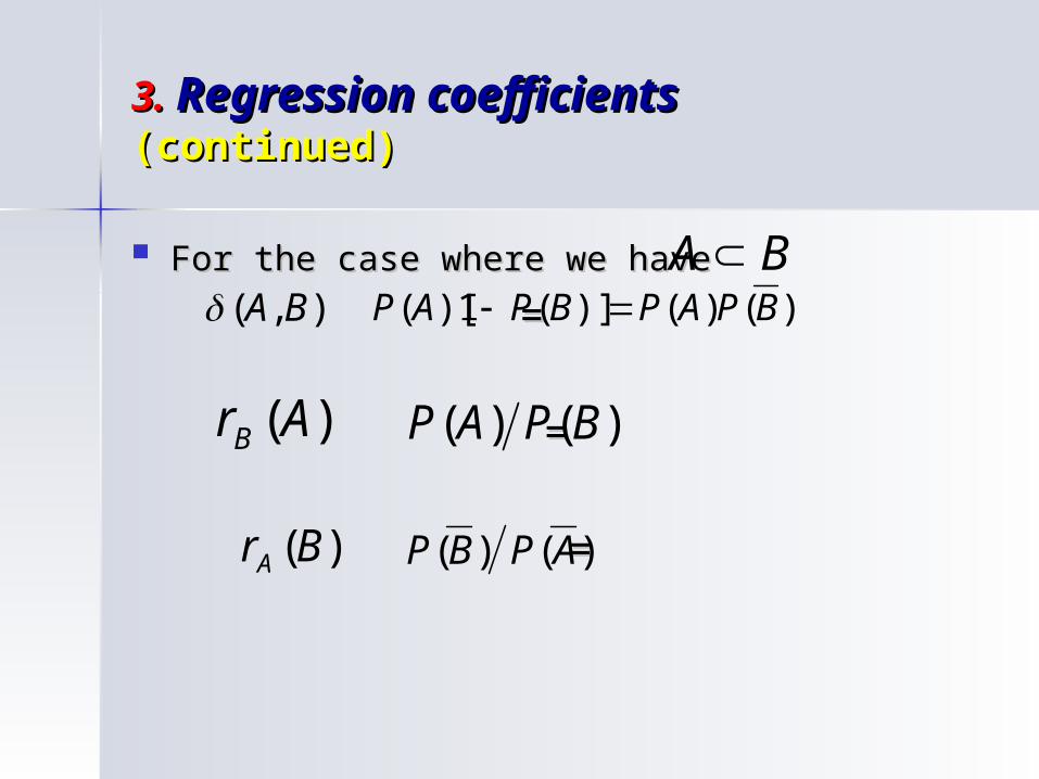
For the case whereFor the case where we havewe have

= =

==

==

BA),( BA )()()](1)[( BPAPBPAP

)(ArB )()( BPAP

)(BrA )()( APBP


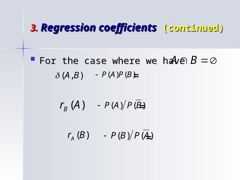
For the case whereFor the case where we havewe have

= =

==

==

),( BA )()( BPAP

)(ArB )()( BPAP

)(BrA )()( APBP

BA


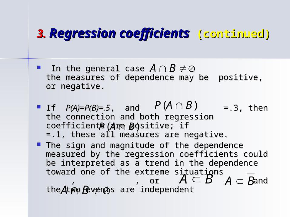
In the general case the measures In the general case the measures of dependence may be positive, or negative. of dependence may be positive, or negative.

If If Р(А)=Р(В)=.5Р(А)=Р(В)=.5, , andand =.3=.3, then the , then the connection and both regression coefficients are connection and both regression coefficients are positive; if positive; if =.1 =.1, these all measures are , these all measures are negative. negative.

The sign The sign and magnitude of and magnitude of the dependence the dependence measured by the regression coefficients measured by the regression coefficients could be could be interpreted as a trend in the dependence toward interpreted as a trend in the dependence toward one of the extreme situations one of the extreme situations , , , , or or and the two events are and the two events are independent independent

BA

)( BAP

)( BAP

BA BA BA


Example 1 (continued): Example 1 (continued): We calculate here We calculate here the two regression coefficients the two regression coefficients and and according to the data of Example 1. according to the data of Example 1.

The regression coefficient of the significant The regression coefficient of the significant increase of the gas prices on the market (event increase of the gas prices on the market (event A), in regard to the significant increase in the A), in regard to the significant increase in the Money Market return (event B) has a numerical Money Market return (event B) has a numerical valuevalue

==(.016)/[(.05)(.95)] = .3368 (.016)/[(.05)(.95)] = .3368 In the same time we have In the same time we have

= = (.016)/[(.08)(.92)] = .2174 .(.016)/[(.08)(.92)] = .2174 .

)(ArB )(BrA

)(ArB

)(BrA

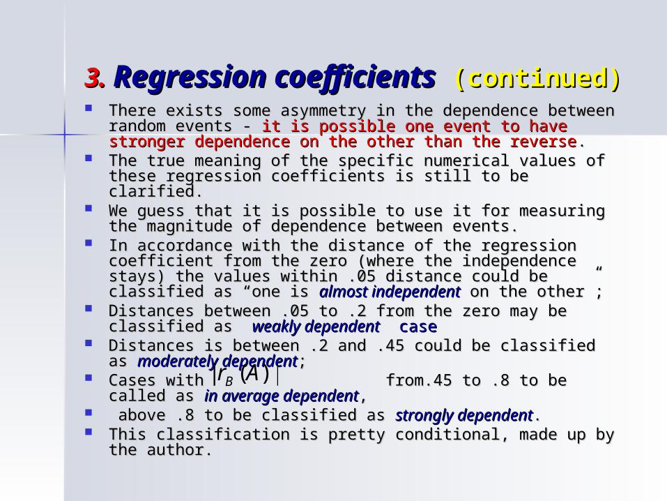
3. 3. Regression coefficients Regression coefficients (continued)(continued) There exists some asymmetry in the dependence between There exists some asymmetry in the dependence between

random events - random events - it is possible one event to have stronger it is possible one event to have stronger dependence on the other than the reversedependence on the other than the reverse. .

The true meaning of the specific numerical values of these The true meaning of the specific numerical values of these regression coefficients is still to be clarified. regression coefficients is still to be clarified.

We guess that it is possible to use it for measuring the We guess that it is possible to use it for measuring the magnitude of dependence between events.magnitude of dependence between events.

In accordance with the distance of the regression coefficient In accordance with the distance of the regression coefficient from the zero (where the independence stays) the values from the zero (where the independence stays) the values within .05 distance could be classified as “one is within .05 distance could be classified as “one is almost almost independentindependent on the other”; on the other”;

Distances between .05 to .2 from the zero may be classified Distances between .05 to .2 from the zero may be classified as as weakly dependentweakly dependent case case

Distances is between .2 and .45 could be classified as Distances is between .2 and .45 could be classified as moderately dependentmoderately dependent;;

Cases with from.45 to .8 to be called as Cases with from.45 to .8 to be called as in in average dependentaverage dependent, ,

above .8 to be classified as above .8 to be classified as strongly dependentstrongly dependent. . This classification is pretty conditional, made up by the This classification is pretty conditional, made up by the

author. author.

|)(| ArB


The regression coefficients satisfy the inequalitiesThe regression coefficients satisfy the inequalities

These also are called Freshe-Hoefding These also are called Freshe-Hoefding inequalities.inequalities.

)(1

)(1,)(

)(min)(

)(

)(1,)(1

)(max

AP

BP

AP

BPBr

AP

BP

AP

BPA

)(1

)(1')(

)(min)(

)(

)(1,)(1

)(max

BP

AP

BP

APAr

BP

AP

BP

APB

4. 4. Correlation between two random Correlation between two random

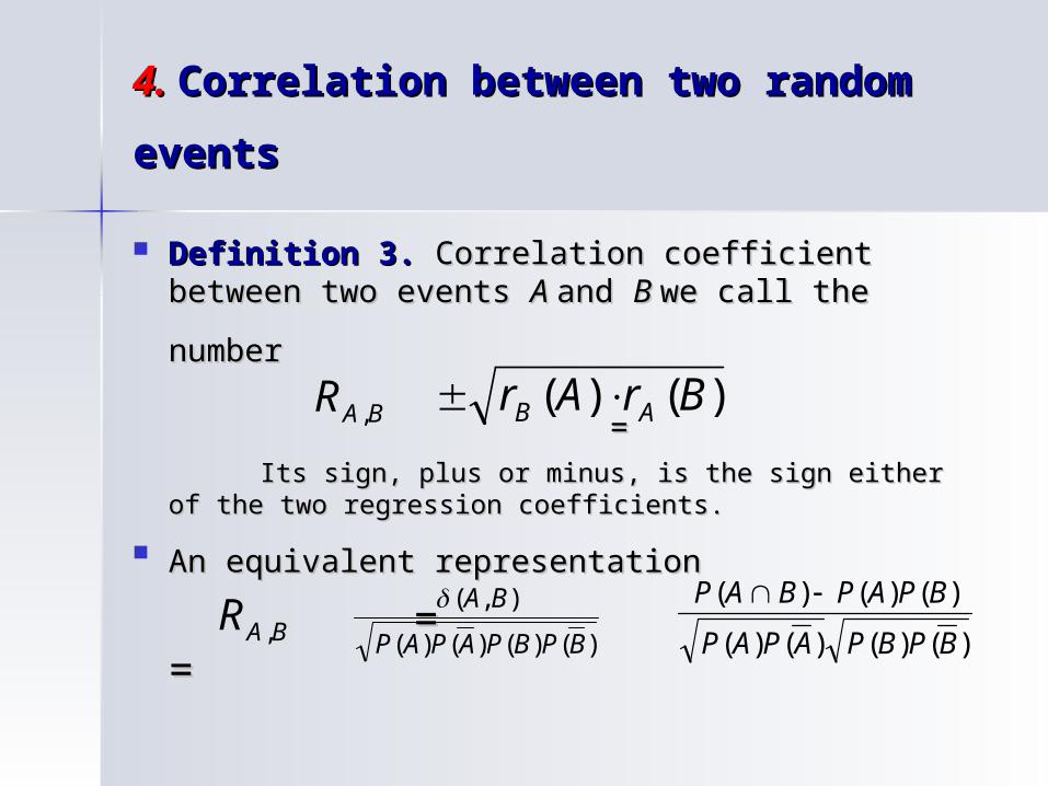
eventsevents Definition Definition 3.3. Correlation coefficient between Correlation coefficient between

two eventstwo events A A and and B B we call the numberwe call the number

== Its sign, plus or minus, is the sign either of the two Its sign, plus or minus, is the sign either of the two

regression coefficients. regression coefficients.

An equivalent representationAn equivalent representation

= = = =

BAR , )()( BrAr AB

BAR , )()()()(

),(

BPBPAPAP

BA

)()()()(

)()()(

BPBPAPAP

BPAPBAP

4. 4. Correlation Correlation (continued)(continued) Remark Remark 3.3. The correlation coefficient The correlation coefficient between the events between the events АА

and and ВВ equals to the correlation coefficient equals to the correlation coefficient between the indicators of the two random events between the indicators of the two random events A A and and B .B .

PropertiesProperties

R1.R1. It is fulfilled It is fulfilled = 0 = 0 if and only if the two eventsif and only if the two events А and В А and В are independent.are independent.

R2.R2. The correlation coefficientThe correlation coefficient always is a number between –1 and always is a number between –1 and +1, i.e. it is fulfilled -1+1, i.e. it is fulfilled -1≤ ≤ ≤ 1.≤ 1.

RR2.1.2.1. The equalityThe equality toto 1 holds if and only if 1 holds if and only if the events the events А А and and В В are are equivalent, i.e. when equivalent, i.e. when АА = В. = В.

RR2.2.2.2. The equalityThe equality toto - 1 - 1 holds holds if and only if if and only if the events the events А А and are and are equivalentequivalent

BAR ,

BAR ,

BA II ,

BAR ,

B

4. 4. Correlation Correlation (continued)(continued)

RR3.3. The correlation coefficientThe correlation coefficient has the same sign as the has the same sign as the other measures of the dependence between two random other measures of the dependence between two random eventsevents А А and and В В , , and this is the sign of the connectionand this is the sign of the connection..

R4R4.. The knowledge of The knowledge of allows calculating the allows calculating the posteriorposterior probability of one of the events under the probability of one of the events under the condition that the other one is occurred. For instance,condition that the other one is occurred. For instance, PP((BB | | AA) will be determined by the rule ) will be determined by the rule

= P(B) = P(B) + +

The net increase, or decrease in the posterior probability The net increase, or decrease in the posterior probability compare to the prior probability equals to the quantity compare to the prior probability equals to the quantity added to P(B)added to P(B),, and depends only on the value of the and depends only on the value of the mutual correlation. mutual correlation.

BAR ,

)|( ABP )(

)()()(, AP

BPBPAPR BA


= = - -

R5R5.. It is fulfilledIt is fulfilled = = - ; = = = - ; =

R6R6..

R7R7.. Particular CasesParticular Cases.. When When , , then then

; If then ; If then

)|( ABP )(BP)(

)()()(,

AP

BPBPAPR BA

BAR

, BAR

, BAR , BAR ,BA

R,

;1, AAR ;1,

AA

R 0,, ASA RR

BA

)()(

)()(,

BPAP

BPAPR BA BA

)()(

)()(,

BPAP

BPAPR BA


The use of the numerical values of the The use of the numerical values of the correlation coefficient is similar to the correlation coefficient is similar to the use of the two regression coefficients. use of the two regression coefficients.

As closer is As closer is to the zero, as to the zero, as “closer” are the two events “closer” are the two events АА and and ВВ to to the independence. the independence.

Let us note once again that Let us note once again that = 0 = 0 if if and only if the two events are and only if the two events are independentindependent. .

BAR ,

BAR ,


As closer is As closer is to to 1, 1, as “dense one within the other” as “dense one within the other” are the events are the events АА andand В,В, and whenand when = 1= 1, the two , the two events coincide (are equivalent).events coincide (are equivalent).

As closer is As closer is to - to -1, 1, as “dense one within the as “dense one within the other” are the events other” are the events АА andand ,, and whenand when = - 1 = - 1 the two events coincide (are equivalent). the two events coincide (are equivalent).

These interpretations seem convenient when These interpretations seem convenient when conducting research and investigations associated with conducting research and investigations associated with qualitative (non-numeric) factors and characteristics. qualitative (non-numeric) factors and characteristics.

Such studies are common in sociology, ecology, Such studies are common in sociology, ecology, jurisdictions, medicine, criminology, design of jurisdictions, medicine, criminology, design of experiments, and other similar areas. experiments, and other similar areas.

BAR ,

BAR ,

BAR ,

BAR ,B


Freshe-Hoefding inequalities for the Freshe-Hoefding inequalities for the Correlation CoefficientCorrelation Coefficient

)()(

)()(,)()(

)()(min),(

)()(

)()(,)()(

)()(max

BPAP

BPAP

BPAP

BPAPBAR

BPAP

BPAP

BPAP

BPAP


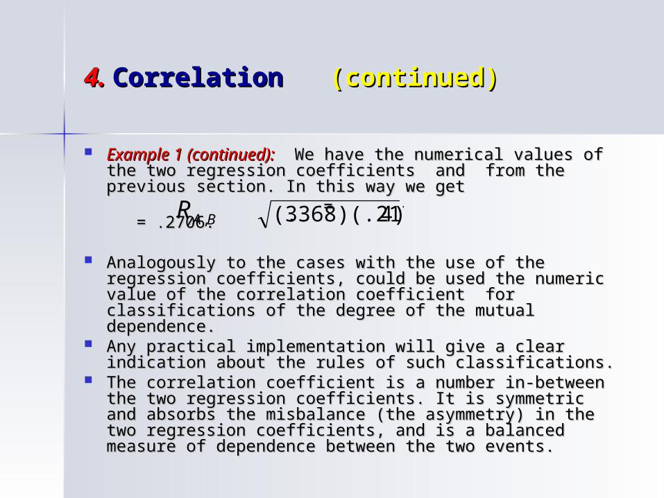
Example Example 1 (1 (continuedcontinued):): We have the numerical values We have the numerical values of the two regression coefficients of the two regression coefficients and and from the from the previous sectionprevious section. . In this way we getIn this way we get

= = = = ..2706.2706.

Analogously to the cases with the use of the Analogously to the cases with the use of the regression coefficients, could be used the numeric regression coefficients, could be used the numeric value of the correlation coefficient for classifications value of the correlation coefficient for classifications of the degree of the mutual dependenceof the degree of the mutual dependence. .

Any practical implementation will give a clear Any practical implementation will give a clear indication about the rules of such classifications. indication about the rules of such classifications.

The correlation coefficient is a number in-between the The correlation coefficient is a number in-between the two regression coefficients. It is symmetric and two regression coefficients. It is symmetric and absorbs the misbalance (the asymmetry) in the two absorbs the misbalance (the asymmetry) in the two regression coefficients, and is a balanced measure of regression coefficients, and is a balanced measure of dependence between the two events.dependence between the two events.

BAR , 4)3368)(.217(.


Examples can be given in variety areas of our Examples can be given in variety areas of our life. For instance: life. For instance:

Consider the possible degree of dependence Consider the possible degree of dependence between tornado touch downs in Kansas between tornado touch downs in Kansas (event (event AA), and in Alabama (event ), and in Alabama (event BB)). .

In sociology a family with 3, or more children In sociology a family with 3, or more children (event (event AA), and an income above the average ), and an income above the average (event (event BB); );

In medicine someone gets an infarct (event In medicine someone gets an infarct (event AA), ), and a stroke (event and a stroke (event BB)). .

More examples, far better and meaningful are More examples, far better and meaningful are expected when the revenue of this approach expected when the revenue of this approach is assessed. is assessed.

AT

5. Empirical estimations 5. Empirical estimations The measures of dependence The measures of dependence

between random events are between random events are made of their probabilities. It made of their probabilities. It makes them very attractive makes them very attractive and in the same time easy for and in the same time easy for statistical estimation and statistical estimation and practical use. practical use.

5. Empirical Estimations5. Empirical Estimations (contd)(contd)

Let in Let in N N independent experiments independent experiments (observations) (observations) the random event the random event АА occurs occurs times, the random event times, the random event ВВ occurs occurs times, and the event times, and the event

occurs times. Then statistical occurs times. Then statistical estimators of our measures of dependence estimators of our measures of dependence will be respectively:will be respectively:

AkBk

BA BAk

N

k

N

k

N

kBA BABA ),(̂


The estimators of the two regression coefficients areThe estimators of the two regression coefficients are ; =; =

The correlation coefficient has estimatorThe correlation coefficient has estimator

= =

)(ˆ BrA)1(

N

k

N

kN

k

N

k

N

k

AA

BABA

)(ˆ ArB)1(

N

k

N

kN

k

N

k

N

k

BB

BABA

),(ˆ BAR)1()1(

N

k

N

k

N

k

N

kN

k

N

k

N

k

BBAA

BABA


Each of the three estimators may be simplified Each of the three estimators may be simplified when the fractions in numerator and when the fractions in numerator and denominator are multiplied by , we will not get denominator are multiplied by , we will not get into detail.into detail.

The estimators are all consistent; the estimator The estimators are all consistent; the estimator of the connection of the connection δ(δ(АА,,ВВ) ) is also unbiased, i.e. is also unbiased, i.e. there is no systematic error in this estimate.there is no systematic error in this estimate.

The proposed estimators can be used for The proposed estimators can be used for practical purposes with reasonable practical purposes with reasonable interpretations and explanations, as it is shown interpretations and explanations, as it is shown in our discussion, and in our example.in our discussion, and in our example.

6.6. Some warningsSome warningsand some recommendationsand some recommendations

The introduced measures of dependence between The introduced measures of dependence between random events are not transitive. random events are not transitive.

It is possible that It is possible that АА is positively associated with is positively associated with BB, , and this event and this event В В to be positively associated with a to be positively associated with a third event third event СС, , but the event but the event АА to be negatively to be negatively associated with associated with СС. .

To see this imagine To see this imagine АА and and ВВ compatible (non-empty compatible (non-empty intersection) as well as intersection) as well as ВВ and and СС compatible, while compatible, while АА and and СС being mutually exclusive, and therefore, with a being mutually exclusive, and therefore, with a negative connection. negative connection.

Mutually exclusive events have negative connection;Mutually exclusive events have negative connection; For non-exclusive pairs For non-exclusive pairs ((А, ВА, В)) and and ( (В, СВ, С)) every kind every kind

of dependence is possible. of dependence is possible.

6.6. Some warnings and some Some warnings and some recommendations recommendations (contd)(contd)

One can use the measures of dependence One can use the measures of dependence between random events to compare degrees of between random events to compare degrees of dependence. dependence.

We recommend the use of Regression We recommend the use of Regression Coefficient for measuring degrees of Coefficient for measuring degrees of dependence. dependence.

For instance, let For instance, let

then we say that the then we say that the event event АА has stronger has stronger association with association with СС compare to its association with compare to its association with BB. .

In a similar way an entire rank of association of any fixed In a similar way an entire rank of association of any fixed event can be given with any collection of other events.event can be given with any collection of other events.

|)(||)(| ArAr CB

77. . An illustration of possible An illustration of possible applicationsapplications

Alan Agresti Categorical Data Analysis, 2006. Alan Agresti Categorical Data Analysis, 2006. Table 1: Observed Frequencies of Income and Table 1: Observed Frequencies of Income and

Job SatisfactionJob SatisfactionJob SatisfactionJob Satisfaction

Income US $$Very

DissatisfiedLittle

SatisfiedModerate

ly Satisfied

Very Satisfied

Total Marginal

ly

< 6,000 20 24 80 82 206

6,000–15,000 22 38 104 125 289

15,000-25,000 13 28 81 113 235

> 25,000 7 18 54 92 171

Total Marginally

62 108 319 412 901

jiji PPP ...,, ,

77. . An illustration … An illustration … (contd)(contd)

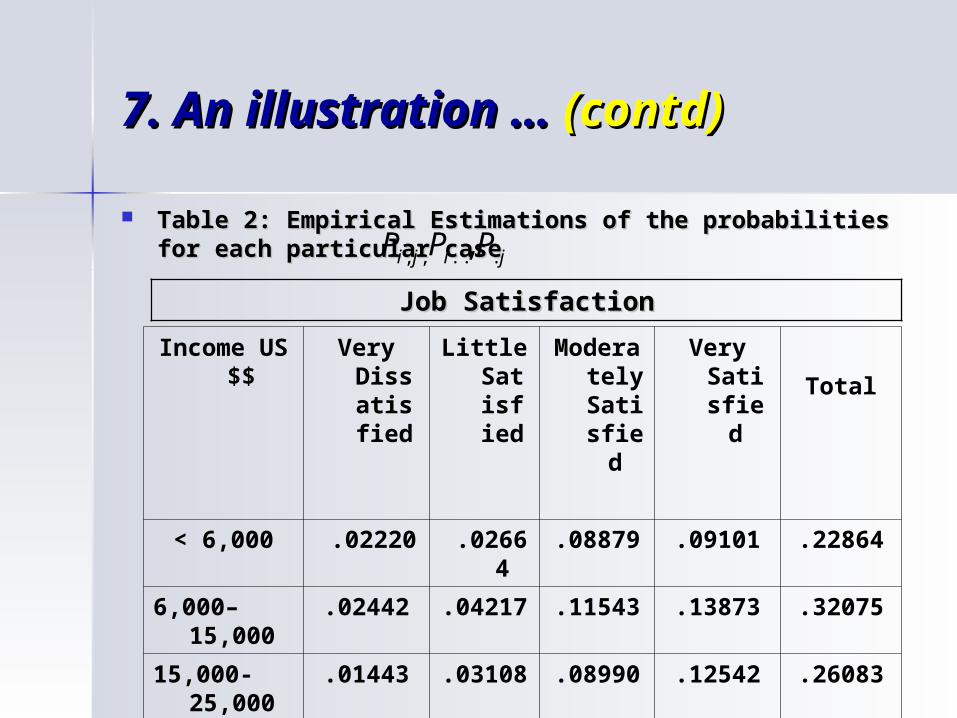
Table 2: Empirical Estimations of the probabilities for Table 2: Empirical Estimations of the probabilities for each particular caseeach particular case

Job SatisfactionJob Satisfaction

Income US $$

Very Dissatisfied

Little Satisfied

Moderately

Satisfied

Very Satisfi

ed

Total

< 6,000 .02220 .02664 .08879 .09101 .22864

6,000–15,000 .02442 .04217 .11543 .13873 .32075

15,000-25,000 .01443 .03108 .08990 .12542 .26083

> 25,000 .00776 .01998 .05993 .10211 .18978

Total .06881 .11987 .35405 .45727 1.00000

jiji PPP ...,, ,


Table 3: Empirical Estimations of the connection function for each Table 3: Empirical Estimations of the connection function for each particular category of Income and Job Satisfactionparticular category of Income and Job Satisfaction

Job SatisfactionJob Satisfaction

Income US $$

Very Dissatisfied

Little Satisfied

Moderately

Satisfied

Very Satisfied

Total

< 6,000 0.006467

-.0007

7

0.00784 -0.01354 0

6,000–15,000 0.0023491

0.003720.0037222

0.001860.001868 8

-0.00794-0.00794 0

15,000-25,000 -0.003517 --0.00019 0.00019

--0.00245 0.00245

0.00615 0.00615 0

> 25,000 -0.005298 --0.00277 0.00277

--0.00726 0.00726

0.015320.015329 9

0

Total 0 0 0 0 0


Surface of the Connection Function (Z variable), Surface of the Connection Function (Z variable), between Income level (Y variable) and the Job between Income level (Y variable) and the Job Satisfaction Level (X variable) , according to Satisfaction Level (X variable) , according to Table 3. Table 3.

1 2 3 4

S1

S3-0.015-0.01

-0.0050

0.0050.01

0.015

0.02

Connection values

Income Level

Satisfaction Level

Connection Function between Income Levesl and Satisfaction Levels

Series1

Series2

Series3

Series4


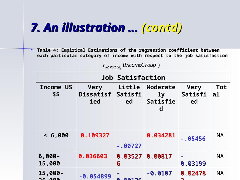
Table 4: Empirical Estimations of the regression coefficient between Table 4: Empirical Estimations of the regression coefficient between each particular category of income with respect to the job satisfactioneach particular category of income with respect to the job satisfaction

Job SatisfactionJob SatisfactionIncome US $

$Very

DissatisfiedLittle

SatisfiedModerately Satisfied

Very Satisfied

Total

< 6,000 0.109327 -.0072

7

0.034281

-.05456 NA

6,000–15,000 0.036603 0.035270.0352766

0.00817 0.00817 -0.03199-0.03199 NA

15,000-25,000 -

0.054899 --0.00176 0.00176

-0.0107-0.0107 0.024780.0247822

NA

> 25,000 -0.005298

--0.02625 0.02625

-0.03175-0.03175 0.061760.0617611

NA

Total 0 0 0 0 0

( )jSatisfaction ir IncomeGroup


Surface of the Regression CoefficientSurface of the Regression Coefficient

Function Function

( )jSatisfaction ir IncomeGroup

1 2 3 4S1

S3-0.1

-0.05

0

0.05

0.1

0.15

Regr. Coeff. values

Satisfaction Level

Income Level

Regression Coefficients of Sattisfaction w.r. to Income Level

Series1

Series2

Series3

Series4


Table 5: Empirical Estimations of the regression coefficient between each Table 5: Empirical Estimations of the regression coefficient between each particular category of the job satisfaction with respect to the income particular category of the job satisfaction with respect to the income groupsgroups


$Very

DissatisfiedLittle

SatisfiedModerately Satisfied

Very Satisfied

Total

< 6,000 0.036670 -

0.00435 0.04445 -.0767

7 0

6,000–15,000 0.010783 0.0170820.017082 0.0085760.008576 --0.036440.03644

0

15,000-25,000 -0.018246

-0.00096-0.00096 -0.01269-0.01269 0.03160.0316 0

> 25,000 -0.034460

-0.01801 -0.01801 -0.04723-0.04723 0.099590.0995944

0

Total NA NA NA NA 0

( )iIncomeGroup jr Satisfaction


Surface of the Regression Coefficient Surface of the Regression Coefficient Function, according to Table 5.Function, according to Table 5.

( )iIncomeGroup jr Satisfaction

1 2 3 4S1

S4-0.1

-0.05

0

0.05

0.1

Regr. Coeff. values

Satisfaction Level

Income Level

Regression Coefficients surface for Satisfaction w.r.to Income

Series1

Series2

Series3

Series4


Table 6: Empirical Estimations of the correlation coefficient between Table 6: Empirical Estimations of the correlation coefficient between each particular income group and the categories of the job satisfactioneach particular income group and the categories of the job satisfaction


$Very

DissatisfiedLittle

SatisfiedModerate

ly Satisfied

Very Satisfied

Total

< 6,000 0.060838 -

0.005623 0.0390

4 -.0647

2 NA

6,000–15,000 0.019883 0.0245480.024548 0.008370.0083711

--0.034140.03414

NA

15,000-25,000 -0.031649

-0.001302-0.001302 --0.011650.01165

0.028110.0281177

NA

> 25,000 -0.053363

-0.02174-0.02174 --0.038720.03872

0.078740.0787422

NA

Total NA NA NA NA NA


Surface of the Correlation Surface of the Correlation

Coefficient Function according to Table 6.Coefficient Function according to Table 6.

( , )i jR IncomeGroup Satisfaction

1 2 3 4S1

S4-0.1

-0.05

0

0.05

0.1

Correlation values

Income Level

Job Satisfaction

Correlation Function for the Income Level and the Job Satisfaction Levels

Series1

Series2

Series3

Series4

77. . An illustration … An illustration … (contd)(contd)A prediction of the Income groupA prediction of the Income group … … Table 7: Table 7: Forecast of the probabilities P(A|B) =P(A)+ δ(A,B)/P(B) of Forecast of the probabilities P(A|B) =P(A)+ δ(A,B)/P(B) of

particular income group given the categories of the job satisfactionparticular income group given the categories of the job satisfaction


$Very

DissatisfiedLittle

SatisfiedModerately

SatisfiedVery

Satisfied Prior P(A)

< 6,000 0.32258 0.2222

3 0.25079 0.25079 0.19900.1990

3 3 .2286

4 6,000–15,000 0.35484 0.351840.35184 0.326010.32601 0.30330.3033

99.3207

5 15,000-25,000 0.20968 0.16668 0.16668 0.253930.25393 0.27420.2742

88 .2608

3 > 25,000 0.11289 0.166660.16666 0.16927 0.16927 0.22320.2232

99 .1897

8

Total 1.00 1.00 1.00 1.00 1.00

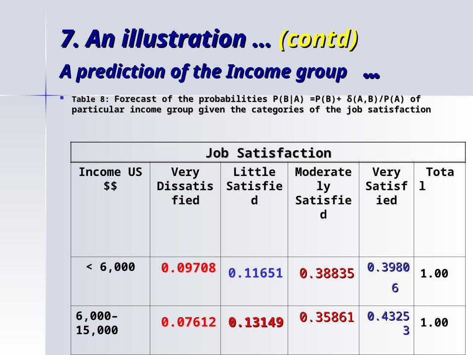
77. . An illustration … An illustration … (contd)(contd)A prediction of the Income groupA prediction of the Income group … … Table 8: Table 8: Forecast of the probabilities P(B|A) =P(B)+ δ(A,B)/P(A) of Forecast of the probabilities P(B|A) =P(B)+ δ(A,B)/P(A) of

particular income group given the categories of the job satisfactionparticular income group given the categories of the job satisfaction


$Very

DissatisfiedLittle

SatisfiedModerately

SatisfiedVery

Satisfied Total

< 6,000 0.09708 0.1165

1 0.388350.38835 0.39800.3980

66 1.00

6,000–15,000 0.07612

0.13140.1314

99

0.358610.35861 0.43250.432533

1.00

15,000-25,000 0.55317 0.07660.076600

0.344680.34468 0.48080.4808

55 1.00

> 25,000 0.02093 0.105260.10526 0.31579 0.31579 0.53800.538022

1.00

Total .06881 .11987 .35405 .45727 1.00

6. CONCLUSIONS6. CONCLUSIONS

We discussed four measures of dependence between two random events.

These measures are equivalent, and exhibit natural properties.

Their numerical values may serve as indication for the magnitude of dependence between random events.

These measures provide simple ways to detect independence, coincidence, degree of dependence.

If either measure of dependence is known, it allows better prediction of the chance for occurrence of one event, given that the other one occurs.

If applied to the events A=[X<x], and B=[Y<y], these measures immediately turn into measures of the LOCAL DEPENDENCE between the r.v.’s X and Y associated with the point (x,y) on the plane.

ReferencesReferences

[1][1] A. Agresti (2006) A. Agresti (2006) Categorical Data AnalysisCategorical Data Analysis, , John Wiley & Sons, Hew York. John Wiley & Sons, Hew York.

[2] [2] B. Dimitrov, and N. Yanev B. Dimitrov, and N. Yanev (1991) (1991) Probability and Probability and StatisticsStatistics, , A textbook, Sofia University “Kliment A textbook, Sofia University “Kliment OhridskiOhridski”, ”, SofiaSofia ( (SecSecооnd Edition 1998, Third Edition nd Edition 1998, Third Edition 2007).2007).

[3] N. Obreshkov [3] N. Obreshkov (1963) (1963) Probability TheoryProbability Theory, , Nauka i Nauka i Izkustvo, Sofia (in Bulgarian). Izkustvo, Sofia (in Bulgarian).

[[44] ] Encyclopedia of Statistical Sciences Encyclopedia of Statistical Sciences (1981 – (1981 –

1988), 1988), v. 1 – v. 9.v. 1 – v. 9. Editors-in-Chief S. Kotz and N. L. Editors-in-Chief S. Kotz and N. L. Johnson, John Wiley & Sons, New York Johnson, John Wiley & Sons, New York ..

References References (contd)(contd)

Genest, C. and Boies, J. (2003). Testing dependence with Kendall plots. The American Statistician 44, 275-284.

Kolev, N., Goncalves, M. and Dimitrov, B. (2007). On Sibuya's dependence function. Submitted to Annals of the Institute of Statistical Mathematics (AISM).

Kotz, S. and Johnson, N., Editors-in-Chief (1982 - 1988). Encyclopedia of Statistical Sciences, v. 1 - v. 9. Wiley & Sons.

Nelsen, R. (2006). An Introduction to Copulas. 2nd Edition, Springer, New York.

References References (contd)(contd)

Schweitzer, B. and Wol, E.F. (1981). On non-parametric measures of dependence, Ann. of Statistics 9, 879-885.

Sibuya, M. (1960). Bivariate extreme statistics. Annals of the Institute of Statistical Mathematics 11, 195-210.

Sklar, A. (1959). Fonctions de repartition a n dimensions et leurs marges. Publ. Inst.

Statist. Univ. Paris 8, 229-331.

Dependence and Measuring of Its Magnitudes Boyan Dimitrov Math Dept. Kettering University, Flint,...

Documents

Transcript of Dependence and Measuring of Its Magnitudes Boyan Dimitrov Math Dept. Kettering University, Flint,...