DEPARTMENT OF MECHANICAL ENGINEERING -...
87
PORTO 2014 Full analysis of suspension geometry and chassis performance of Formula Student racing car AUTHOR: Miłosz Kowalik DEPARTMENT OF MECHANICAL ENGINEERING MASTER THESIS SUPERVISION: Fernando Jose Ferreira
Transcript of DEPARTMENT OF MECHANICAL ENGINEERING -...

PORTO 2014
Full analysis of suspension geometry and
chassis performance of Formula Student
racing car
AUTHOR: Miłosz Kowalik
DEPARTMENT OF MECHANICAL ENGINEERING
MASTER THESIS
SUPERVISION: Fernando Jose Ferreira

2

3
TABLE OF CONTENT
1. INTRODUCTION .............................................................................................................. 9
1.1 BACKGROUND ......................................................................................................... 9
1.2 GOALS ........................................................................................................................ 9
2. DOUBLE WISHBONE SUSPENSION (SLA) ................................................................ 10
3. SUSPENSION GEOMETRY PARAMETERS ................................................................ 11
3.1. WHEELBASE AND TRACK WIDTH .................................................................... 11
3.2. KINGPIN INCLINATION ANGLE AND OFFSET ................................................ 12
3.3. CASTER AND CASTER TRAIL ............................................................................. 13
3.4. ROLL CENTERS AND ROLL AXIS ....................................................................... 14
3.5. TIRES SIDE FORCES DISTRIBUTION ................................................................. 15
3.5.1. Slip angle ............................................................................................................ 15
3.5.2. Lateral load transfer ........................................................................................... 17
3.6. CAMBER .................................................................................................................. 18
3.7. CAMBER THRUST .................................................................................................. 20
3.8. TOE ANGLE ............................................................................................................. 21
3.9. ANTI-DIVE AND ANTI-SQUAT ............................................................................ 22
4. SUSPENSION GEOMETRY DESIGN PROCESS ......................................................... 24
5. VIRTUAL MODEL FOR SUSPENSION ANALYSIS ................................................... 27
6. SUSPENSION GEOMETRY GOALS CONSIDERATIONS AND RESULTS
ANALYSIS .............................................................................................................................. 32
6.1. KINGPIN POSITIONING ANALYSIS .................................................................... 32
6.1.1. Caster and kingpin inclination ............................................................................ 32
6.1.2. Results analysis .................................................................................................. 33
6.1.3. Conclusions ........................................................................................................ 34
6.2. FRONT VIEW GEOMETRY ANALYSIS ............................................................... 36
6.2.1. Roll centers ......................................................................................................... 36
6.2.2. Results analysis – roll centers ............................................................................ 37
6.2.3. Camber gain ....................................................................................................... 38
6.2.4. Results analysis – camber gain ........................................................................... 39
6.2.5. Track width change and bump steering .............................................................. 40
6.2.6. Results analysis - track width change and bump steering .................................. 42
6.2.7. Conclusions ........................................................................................................ 43
6.3. SIDE VIEW GEOMETRY ANALYSIS ................................................................... 46
6.3.1. Anti features ....................................................................................................... 46
6.3.2. Results analysis - anti features ........................................................................... 46
6.3.3. Conclusions ........................................................................................................ 47

4
7. FRAME PERFORMANCE TESTS AND GOALS ......................................................... 49
8. RIGID CHASSIS CASE ................................................................................................... 51
9. TESTS PROCEEDINGS .................................................................................................. 56
10. FINITE ELEMENTS ANALYSIS ................................................................................ 57
10.1 MODEL CREATION ................................................................................................ 57
10.2 FIXTURE AND LOAD APPLICATION ................................................................. 59
10.3 VIRTUAL FRAME TEST ........................................................................................ 62
10.4 VIRTUAL CHASSIS TEST ...................................................................................... 67
10.5 CHASSIS IMPROVEMENTS .................................................................................. 71
11. EXPERIMENTAL TESTS ........................................................................................... 74
11.1 TORSIONAL STIFFNESS TEST ............................................................................. 74
11.2 STRESS TEST .......................................................................................................... 77
11.3 EXPERIMENTAL FRAME TESTS RESULTS ....................................................... 79
11.4 EXPERIMENTAL CHASSIS TESTS RESULTS .................................................... 81
12. CONCLUSIONS ........................................................................................................... 85
13. REFERENCES .............................................................................................................. 87

5
TABLE OF FIGURES
Fig. 1.1 The car in June 2014 and the virtual model actual in February 2014. 9
Fig. 2.1. Short Long Arm suspension with push rod of analyzed vehicle. 10
Fig. 3.1. Wheelbase 11
Fig. 3.2. Track width 11
Fig. 3.3. Wheelbase and track width changes with wheel travel. 12
Fig. 3.4. Relation between track width changes (scrub changes) and IC location 12
Fig. 3.5. Kingpin inclination and scrub radius (both are positive in this example) 12
Fig. 3.6. Negative caster angle and caster offset with 0 spindle offset (left) and positive
camber angle and offset with negative spindle offset. 13
Fig. 3.7. Roll center and roll axis 14
Fig. 3.8. Determining roll center 14
Fig. 3.9. Jacking effect 15
Fig. 3.10. Slip angle and tire’s deformation at contact patch with road. 15
Fig. 3.11. Example relation between lateral force and slip angle 16
Fig. 3.12. Lateral force and vertical load relation for different slip angles 16
Fig. 3.13. Example relation between vertical load on tire and lateral force generated with 5°
slip angle. 16
Fig. 3.14.Roll of a car in cornering. Force analysis. 17
Fig. 3.15. Single axis force analysis. 18
Fig. 3.16. Positive and negative camber. 18
Fig. 3.17. Concept of instant center. 19
Fig. 3.18. Relation between camber change rate and fvsa length. 19
Fig. 3.19. Mechanism of camber generating lateral force 20
Fig. 3.20. Cambered bias-ply tire contact patch distortion. 20
Fig. 3.21. Effect of camber on lateral force – slip angle relation. 21
Fig. 3.22. Peak lateral force vs. camber, P225/70R15 tire. 21
Fig. 3.23. Toe-in and toe-out 22
Fig. 3.24. Free body diagram for calculation of anti-dive 22
Fig. 3.25. Free body diagram for calculating anti-squat of independent rear suspension 23
Fig. 4.1. Wheel packaging 24
Fig. 4.2. Front view control arms configuration design process 25
Fig. 4.3. Process of side view IC location 25
Fig. 4.4. Suspension geometry design process. 26

6
Fig. 5.1. Full suspension model in LSA and SolidWorks. 28
Fig. 5.2. Top and front view of front suspension. SolidWorks model. 28
Fig. 5.3. Front suspension model in LSA. 28
Fig. 5.4. Top and front view of rear suspension. SolidWorks model. 29
Fig. 5.5. Rear suspension model in LSA. 29
Fig. 5.6. Front suspension model in LSA with points numbered 30
Fig. 5.7. Rear suspension model in LSA with points numbered 31
Fig. 6.1. Example of acceptable camber gains with steering (left) and caster gains with bump
travel. 33
Fig. 6.2. Camber changes while turning for analyzed vehicle. 34
Fig. 6.3. Bottom view of lower control arm mounted to upright. 35
Fig. 6.4. Example of acceptable roll center heights changes relatively to ground with bump
travel 36
Fig. 6.5. Roll axis in side view. Front roll center (left) is placed higher above the ground than
the rear. 37
Fig. 6.6. Roll centers’ migration with roll of the vehicle’s body. 37
Fig. 6.7. Roll centers height change with bump travel. 38
Fig. 6.8. Examples of acceptable relation between camber gain and bump travel 39
Fig. 6.9. Camber gain with bump travel for front axis. 39
Fig. 6.10. Camber gain with bump travel for rear axis. 40
Fig. 6.11. Camber loss with body roll for front and rear axis. 40
Fig. 6.12. Example of acceptable track width change with bump travel. 41
Fig. 6.13. Example of wheel that tends to toe-out with jounce and toe-in in rebound. 41
Fig. 6.14. Example of wheel that tends to toe-out both in jounce and rebound, passing through
initial position in ride height. 42
Fig. 6.15. Example of acceptable toe angle change with bump travel. 42
Fig. 6.16. Half track change with bump travel for analyzed vehicle. 43
Fig. 6.17. Toe angle change with bump travel for analyzed vehicle. 43
Fig. 6.18. Single Cardan’s coupling and the steering rack located in front of and above front
axis. 45
Fig. 6.19. Example acceptable values of anti-dive (left) and anti-squat in bump travel 46
Fig. 6.20. Analyzed vehicle’s anti-dive values for front and rear axle changing with bump
travel. 47
Fig. 6.21. Analyzed vehicle’s anti-squat value (rear axle) changing with bump travel 47
Fig. 7.1 Chassis deformation modes 49
Fig. 8.1 Mathematical model for torsional stiffness calculations for rigid chassis case 51
Fig. 8.2 Systems position under the force acting with the ground as reference 51

7
Fig. 8.3 Systems position under the force acting with the frame as reference 52
Fig. 8.4 Force and displacement relations between wheel and spring 52
Fig. 8.5 Mathematical model of case with compliant chassis 54
Fig. 8.6 Relation between chassis and full vehicle torsional stiffness 55
Fig. 9.1 Tests proceedings 56
Fig. 10.1 Original frame model and example change made during manufacturing 57
Fig. 10.2 3D sketch for the simulations model 57
Fig. 10.3 Chassis model prepared for tests and beam structure replacing engine and gearbox 58
Fig. 10.4 Model represented with its nodes and meshed with beam/truss elements 59
Fig. 10.5 Rear suspension bay fixed at suspension mounts and at frame nodes 59
Fig. 10.6 Single plane of rear suspension bay fixed at suspension mounts and at frame nodes 60
Fig. 10.7 Single line of rear suspension bay fixed at suspension mounts and at frame nodes 60
Fig. 10.8 Fixture and load application in front of the car 61
Fig. 10.9 Fixture and load application for full chassis assembly test 61
Fig. 10.10 Vertical dislocations for single line fixed and engine fully mounted 62
Fig. 10.11 Vertical dislocations for experimental test’s boundary conditions 63
Fig. 10.12 Twist angle value along longitudinal axis of the vehicle in frame test 64
Fig. 10.13 Pipes deformation under suspension support. 65
Fig. 10.14 Points, where stress values were measured 66
Fig. 10.15 Points for measuring stress value after placing strain gauges 66
Fig. 10.16 Vertical translation diagram for fully mounted engine case 67
Fig. 10.17 Vertical translation diagram for partially mounted engine case 68
Fig. 10.18 Twist angle value along longitudinal axis of the vehicle 70
Fig. 10.19 Maximum stress in chassis longitudinal torsion test 71
Fig. 10.20 Points for measuring stress value after placing strain gauges – chassis test 71
Fig. 10.21 Forces and/or moments in triangulated and non-triangulated structure. 72
Fig. 10.22 Improvements for torsional stiffness of chassis 72
Fig. 10.23 Vertical displacements for chassis with improvements 73
Fig. 11.1 Engine mounts that were either not welded or not bolted 74
Fig. 11.2 Rear part of the model representing engine not fully mounted 74
Fig. 11.3 Rear and front of the car prepared for frame laboratory tests 75
Fig. 11.4 Scheme of supports loads and displacements in laboratory frame test 76
Fig. 11.5 Scheme of supports loads and displacements in laboratory chassis test 76
Fig. 11.6 Strain gauge and digital indicator used in the tests 77
Fig. 11.7 Combined tension of axial forces and bending in a beam 77

8
Fig. 11.8 Quarter bridge scheme from digital indicator and strain gauges connection 78
Fig. 11.9 Angle and torque relation in laboratory frame test 80
Fig. 11.10 Torsional stiffness determined from torque-angle relation 80
Fig. 11.11 Stress-torque relations in two chosen points of frame 81
Fig. 11.12 Angle and torque relation in laboratory frame test 82
Fig. 11.13 Torsional stiffness determined from torque-angle relation 83
Fig. 11.14 Stress-torque relations in two chosen points of frame for chassis test 83

9
1. INTRODUCTION
1.1 BACKGROUND
Formula Student events gather engineering students, who compete, designing, building and
racing single-seater cars. The team of ISEP is working on its first car that soon will take part
in this competition. This work aims to analyze the current design’s chassis, focusing on
suspension geometry and frame’s performance. After analyzing results of the tests planned
suggestions, that can be taken into consideration during design process of next cars will be
presented. As the car has not been tested yet this work can also be helpful to explain its
performance on the track later.
Fig. 1.1 presents the car’s state in the beginning of June 2014 and the model that was
delivered for virtual tests in February the same year. The car was later undergoing
adjustments even on the last days before the practical experiments. All the changes were taken
into consideration and the results presented refer to the state of the car actual for the day of
the papers presentation.
Fig. 1.1 The car in June 2014 and the virtual model actual in February 2014.
Correct geometry of suspension is necessary to provide good handling of a car. The
requirement for correct behavior of suspension however is also a well designed frame. If it
does not ensure enough rigidity and does not support suspension correctly, it disturbs its
correct functioning. It is therefore important to make sure both these systems work properly.
This work will propose design goals that, if met, ensure good kinematic behavior of the
suspension. Later virtual tests will be prepared and performed in order to compare their results
with the goals set. To verify the results of chassis stiffness tests additional laboratory
experiments will be run.
1.2 GOALS
The goals of this work therefore are set as follows:
Set design targets for suspension geometry and frame
Analyze suspension geometry of the car, using Lotus Suspension Analysis software
Analyze frame behavior, using Finite Elements Method
Verify virtual tests of frame by running laboratory experiments
Compare the results with goals set and propose improvements

10
2. DOUBLE WISHBONE SUSPENSION (SLA)
The suspension used in analyzed vehicle can be classified as Short Long Arm suspension with
push rod. This type of suspension is very commonly used because it allows to design-in
demanded kinematic features, that are the topic of this paper, with less compromise in
comparison with other types. The usage of push rod and placing shock absorbers onboard
decreases unsprung mass.
The suspension system (Fig. 2.1) consists of two A-shaped control arms (upper 1 and lower 2)
of different length in front view of the vehicle, which determine upright 3 path and position in
suspension travel. Steering rod 4 is an element of steering system, which determines upright
position with steering rack 5 travel. Push rod 6 is attached to upright and through rocker 7
transfers suspension movements on shock absorber 8 (spring and damper).
Fig. 2.1. Short Long Arm suspension with push rod of analyzed vehicle. Control arms: upper
– 1, lower – 2, upright – 3, steering rod – 4, steering rack – 5, push rod – 6, rocker – 7, shock
absorber – 8.

11
3. SUSPENSION GEOMETRY PARAMETERS
The following chapter defines and explains all the parameters, dimensions and features that
are crucial for suspension system design and vehicle behavior, that the following part of this
paper refers to. It aims mostly to get the reader acquainted with them, while considerations
about specific values and their influence on sport vehicle are mostly presented with analysis
of results of virtual test in other chapters. The exception here are only camber and roll centers,
that required introducing to the reader additional, more complex questions related to tire
behavior and load transfer.
This chapter can also be referred to as the theoretical basis, that justifies the conclusions and
advices included in analysis of virtual tests’ results.
3.1. WHEELBASE AND TRACK WIDTH
Wheelbase is defined as distance between centers of contact patches of front and rear axis tire
in side view (Fig. 3.1). Long wheelbase decreases vehicle pitch (longitudinal inclination)
while short ensures better maneuverability.
Fig. 3.1. Wheelbase [1]
Track width (Fig. 3.2) is the distance between centers of contact patches of left and right tire
of the same axis in front view. Wider track width reduces body roll. Its value can be different
for front and rear axis.
Fig. 3.2. Track width [2]
Both wheelbase and track width may change with wheel travel and suspension movements
related to its elasticity (Fig. 3.3). As there were no reasons found for wheelbase changes being
included in design goals of a sport vehicle, it is not analyzed in following part of this paper.

12
Fig. 3.3. Wheelbase and track width changes with wheel travel.[2]
The changes of track width depend on the location of instant center of rotation of suspension
in front view (Fig. 3.4; explanations about instant center in chapter about camber). The closer
to ground it is located, the smaller these changes will be.
Fig. 3.4. Relation between track width changes (scrub changes) and IC location [[3]
3.2. KINGPIN INCLINATION ANGLE AND OFFSET
Kingpin inclination is an angle between steering axis and line normal to the road surface in
front view of the car (Fig. 3.5). The distance between points where those two lines intersect
ground surface is called scrub radius or kingpin offset.
Fig. 3.5. Kingpin inclination and scrub radius (both are positive in this example) [2]
Kingpin inclination is positive when the top of steering axis is closer to the centerline of the
vehicle and scrub radius is positive if the steering axis intersects the ground more inboard than
the wheel’s central plane.
Kingpin inclination causes both wheels to drop relatively to body when steering, which lifts
the front of the car, generating force, that sets the wheels back to straight forward position.
Kingpin inclination also causes the wheels to change camber while steering – outer wheel
towards positive values (loose camber) and inner towards negative values.

13
Scrub radius is a lever which produces steering torque related to longitudinal forces from road
on tire.
The values of kingpin inclination and scrub radius are correlated in such way, that decreasing
one increases the other. In order to avoid this kind of compromise changes in packaging of
brakes and upright or a selection of rim with different wheel offset are required.
3.3. CASTER AND CASTER TRAIL
Caster is an angle that steering axis creates with line perpendicular to ground in the side view
of a car (Fig. 3.6). The distance between the point where steering axis intersects the ground
and projection of wheel’s axis on the ground is referred to as caster trail or caster offset.
Although caster angle and offset are related to each other it is possible to obtain any
combination of these values by offsetting wheel axis from steering axis (in side view) in
upright design. The distance between wheel axis and steering axis along ground level is called
spindle offset.
Fig. 3.6. Negative caster angle and caster offset with 0 spindle offset (left) and positive
camber angle and offset with negative spindle offset. [1]
Caster angle is positive when the top of steering axis is leaned backwards (towards rear of the
car). With zero spindle offset it generates positive caster trail (steering axis intersects ground
in front of wheel’s axis projection on the ground). The spindle offset is considered positive if
the steering axis crosses the wheel axis’ level in front of the wheel’s axis.
While steering positive caster angle causes the inner wheel to drop and outer wheel to raise
relatively to body. That is a reason for car’s front’s roll that generates forces setting wheels
back in straight forward position, contributing to kingpin inclination’s similar effect. When it
comes to camber changes though positive caster causes both wheels to lean in the turn
(camber values change towards negative values).
When the wheels are steered, caster trail generates steering torque, caused by lateral forces
acting on the tires’ contact patch, that sets the wheels back to straight forward position.

14
3.4. ROLL CENTERS AND ROLL AXIS
Roll center is a point in a front view of a car which the body rolls around. The line connecting
front and rear axis’ roll centers is the roll axis (Fig. 3.7).
In order to draw roll center of an axis lines connecting center of tire contact patch and IC of
an upright have to be drawn for both – left and right – wheels. The point where these lines
intersect is the roll center (Fig. 3.8). If the suspension is symmetric and no roll is present the
roll center is located on the centerline of the car.
Fig. 3.7. Roll center and roll axis [2]
Fig. 3.8. Determining roll center (RCH – roll center height) [3]
As roll center is an instant center of rotation, its location changes with roll and suspension
travel.
If the CG of the vehicle is subjected to any side forces (ex. centrifugal force while cornering)
a torque around roll axis is generated. This torque’s value depends on the force and the
distance between CG and the roll axis.
Roll center is also related to horizontal-vertical coupling effect of lateral forces acting on tires.
This is often called “jacking effect” and the forces causing it – “jacking forces”. Fig. 3.9
explains how lateral forces generate torque around suspensions’ front view instant center
(whose location is correlated with roll center’s location Fig. 3.8). A lateral force on a tire’s
contact patch with a ground has to act on a line connecting the patch’s center with the IC. It
has to have the vertical force component then and, in case of roll center located above ground,
push the wheel down, under the body and lift the sprung mass.

15
Fig. 3.9. Jacking effect [3]
3.5. TIRES SIDE FORCES DISTRIBUTION
In order to present the influence that the roll centers’ location has on handling of the vehicle it
is necessary to discuss more profoundly tires’ and suspension’s behavior in cornering,
explaining phenomena of slip angle and lateral load transfer.
3.5.1. Slip angle
Slip angle is defined as the angle between tire’s direction of heading (or in practice wheel
center plane) and its actual direction of travel (Fig. 3.10). The reason for discrepancy of these
two directions is the fact that any side force generated by the tire, that is needed to keep the
car in turn, requires it to deform elastically at the contact patch with ground, causing the
change of travel direction.
Fig. 3.10. Slip angle and tire’s deformation at contact patch with road. [1]
That means that for each tire with certain inflation pressure and vertical load a curve of
relation between side force generated and slip angle can be plotted (Fig. 3.11). For changing
vertical load however the side force generated at the same slip angle will be changing too as it
is presented on Fig. 3.12.

16
Fig. 3.11. Example relation between lateral force and slip angle [4]
Fig. 3.12. Lateral force and vertical load relation for different slip angles [4]
From an example relation between vertical load on tires and the lateral force they generate
with constant slip angle (Fig. 3.13) a conclusion can be drawn, that if the vertical load is
distributed equally between tires they generate more lateral force
(760lb each in example) than when a difference between inner and outer tire occurs (680lb per
tire on average). In other words more slip angle is required to generate the same amount of
lateral force.
Fig. 3.13. Example relation between vertical load on tire and lateral force generated with 5°
slip angle. Two tires with distribution of loads 400lb on one and 1200lb on the other generate
on average 680lb lateral force while tire loaded with 800lb generates 760lb. [4]

17
3.5.2. Lateral load transfer
Whenever a car is cornering a centrifugal force directed to the center of the cornering curve
must appear. Being attached to the center of gravity, it causes a moment around roll axis and
makes the car body roll around it. Analysis of this situation is presented in Fig. 3.14.
Assuming small values of ϕ and ε (cos ϕ = cos ε = 1 and sin ϕ = ϕ) the roll angle may be
calculated as [4]:
(Eq. 3.1)
where Kϕ is roll stiffness of an axis, defined as amount of counteracting moment generated by
an axis with 1rad of body roll.
Fig. 3.14.Roll of a car in cornering. Force analysis. [4]
Except for determining car body roll it is important to analyze force diagram on front and rear
axis separately, as it significantly influences lateral load distribution between tires. As any
kind of suspension can be presented as set of two springs, simple diagram of rigid axis
suspension from Fig. 3.15 can be applied in this case for calculations of independent
suspension too (as long as roll stiffness is already given and does not have to be calculated
with respect to the diagram). An equation for equilibrium of moments around roll center can
be solved for the difference between vertical forces on outside and inside tire:
(Eq. 3.2)

18
Fig. 3.15. Single axis force analysis.[4]
It can be noticed that there are two mechanisms that are responsible for load transfer while
cornering. First is related to side forces generating moment around roll center and therefore its
influence on increase of load being transferred grows with roll center height. The other one,
caused by centrifugal force, depends on axis roll stiffness and roll angle, or in other words on
summary roll stiffness of both axis, as it determines roll angle, and its distribution between
front and rear.
3.6. CAMBER
Camber is defined as the angle between wheel’s center plane and a plane perpendicular to the
ground (Fig. 3.16). It is considered positive when the top of the wheel is leaned outboard and
negative, when it is leaned inboard.
Fig. 3.16. Positive and negative camber.
Camber changes with body roll, suspension travel and steer travel. These changes have to be
taken into consideration during design of suspension system, so that camber has demanded
values within all range of vehicle behavior.
The general approach to design of camber changes is that gains related to suspension and steer
travel should compensates for loss related to body roll.
Camber gain rate with suspension travel depends on control arms configuration in front view.
At any given moment the upright rotates around instantaneous center IC, located where
elongations of arms intersect (Fig. 3.17). The position of IC however constantly changes
when arms change their position.

19
Fig. 3.17. Concept of instant center.[3]
The camber change rate depends on the distance between IC and center of the wheel in front
view (fvsa length – front view swing arm length) according to the following equation [3]:
(Eq. 3.3)
It can be concluded that suspensions with front view IC located close to wheels have higher
camber gain rates (Fig. 3.18).
Fig. 3.18. Relation between camber change rate and fvsa length. [3]
As IC travels with changing position of control arms, camber change rate values also vary
with wheel travel. This fact can be used to design demanded shape of camber gain curve.
Shortening upper arm in relation to lower arm causes camber to grow faster in jounce of
suspension and slower in rebound.
Camber changes related to steer travel depend on kingpin positioning and for this reason are
mentioned in following chapters.

20
3.7. CAMBER THRUST
Camber contributes to lateral tire forces due to mechanism presented on Fig. 3.19. Inclined
wheel behaves like a part of a cone rolling on the ground and tends to generate force directed
to the peak of the cone (positive camber outboard and negative camber inboard force). The
side force generated by camber is called camber thrust.
Fig. 3.19. Mechanism of camber generating lateral force [2].
Although mechanism of camber thrust for radial tires (or wide bias-ply tires) is not well
understood it is probably caused by distortions in tire’s tread pattern and side walls and can be
compared to mechanism observed in narrower bias-ply tires (Fig. 3.20). Center line of a
contact patch of a static, cambered tire is curved. When it rolls, however the path of a point
entering the contact patch goes straight along the direction of motion. The sum of the forces
from road causing this kind of tire deformation result in camber thrust.
Fig. 3.20. Cambered bias-ply tire contact patch distortion. [3]
Camber thrust can be generally treated as a separate mechanism, additive with slip angle
generating side force (Fig. 3.21). For higher values of slip angle however the camber thrust
“rolls-off’, which means its additive effect decreases. Nevertheless it causes the maximum
side force generated by tire to grow.

21
Fig. 3.21. Effect of camber on lateral force – slip angle relation. [3]
Tests of tires can indicate the optimum camber value, for which a specific tire model reaches
the best maximum side force. For racing tires it is usually less than 5°. The tests proved also,
that the optimum camber value grows with tire’s vertical load (Fig. 3.22). This relation is
untrue only for lower load values, which the results are probably less reliable for.
Fig. 3.22. Peak lateral force vs. camber, P225/70R15 tire. [3]
3.8. TOE ANGLE
Toe angle is an angle between wheel’s central plane and centerline of the vehicle in top view
(Fig. 3.23). It is called toe-in when the forward distance between wheels is smaller than the aft
distance. In the opposite situation it is called toe-out.

22
Fig. 3.23. Toe-in and toe-out [2]
Some toe angle is introduced in neutral position in order to compensate for steering system
elasticity effects and keep the wheels in straight forward position, reducing rolling resistance.
Toe angle changes with bump travel, depending on steering rod location.
3.9. ANTI-DIVE AND ANTI-SQUAT
Control arms configuration in side view can provide that some portion of force counteracting
weight transfer during accelerating and braking is provided by suspension linkage and not by
springs. That results in less deflection and elongation of springs and reduction of pitch. These
features are called anti-squat (for acceleration) and anti-dive (for braking). Their values are
expressed as percentage that the force delivered by linkage constitutes in whole force
counteracting weight transfer.
Anti features depend on IC of control arms position in side view and therefore their demanded
values have to be considered when this IC is located. Solving free body diagram from
Fig. 3.24 the following equations [3] relating IC position (
, where svsa is
side view swing arm; l – distance between center of tire patch and CG along horizontal axis; h
– CG’s height above ground) and anti-dive can be obtained:
(Eq. 3.4)
And analogically for rear:
(Eq. 3.5)
Fig. 3.24. Free body diagram for calculation of anti-dive [3]

23
In case of anti-squat however two facts have to be paid attention to. First of all
anti-squat can only be considered for driven axis, in this case rear, as while accelerating the
front axis does not generate any horizontal force that could counteract weight transfer. Second
of all for independent suspension torque reaction is not transferred through suspension linkage
and a different free body diagram (Fig. 3.25) should be considered. The resulting equation [3]
is as follows:
(Eq. 3.6)
Fig. 3.25. Free body diagram for calculating anti-squat of independent rear suspension [3]

24
4. SUSPENSION GEOMETRY DESIGN PROCESS
The following chapter presents the process of suspension geometry design presented in [3]. It
focuses mostly on the order of the decisions about dimensions that have to be defined, while
considerations about their specific values and way to calculate or draw them are included in
other parts of that paper.
First general packaging parameters (related to car body size), wheelbase and track width
should be determined. Later on a designer is allowed to proceed with wheel packaging. This
should start with choosing tire size and rim diameter. As the next step a brake caliper should
be located in such way, that enough clearance is maintained between inner surface of the rim.
That automatically determines position of brake rotor. At this point a lower ball joint should
be placed. In order to obtain desired (low) values of kingpin inclination and scrub radius in
following step this joint should be placed possibly outboard. It is generally also advised
because of structural reasons to place it possibly low with, of course, maintaining minimum
clearance with ground and rim.
At that moment values of kingpin inclination and scrub radius are determined (Fig. 4.1). For
rear-wheel-drive cars, as those values are correlated, a low kingpin inclination is set and the
resulting scrub radius has to accepted.
Fig. 4.1. Wheel packaging [3]
A steering rack can be located then. Packaging constraints should be considered and design of
steering system geometry too. Due to compliance effects while cornering it is required to
place the steering rack in front of wheel axis if it is low-mounted and behind it if it is high-
mounted. If so the elasticity related steer angle will cause understeer rather than dangerous
oversteer.
Next step is defining control arms configurations, starting with determining roll center height
and then camber ratio and calculating front view swing arm length as it is described in
previous chapters. This values together with outer ball joints location determine lines on
which control arms are located (Fig. 4.2).

25
Fig. 4.2. Front view control arms configuration design process [3]
Later usually the lower control arm is designed as long as packaging constraints let and the
upper one’s length is shortened until the demanded camber curve is obtained (compare with
chapter 3.6). Designing push rod and rocker should result with spring ratio close to 1:1, which
ensures good stiffness with low weight of design.
The following task is designing side view geometry. Instant centers should be established
first. They should result from decision about demanded anti features, which according to
Eq. 3.4, Eq. 3.5 and Eq. 3.6 determine ϕ, and decision about the shortest acceptable svsa
length (Fig. 4.3). As for rear axis it may be impossible to obtain demanded anti-squat,
anti-dive and svsa length some kind of compromise may be required.
Fig. 4.3. Process of side view IC location [3]
Position of ball joints of upright in side view should be determined too, establishing
demanded caster angle and caster trail.
When both front and side view geometries are ready, what still has to be done is determining
positions of inner ball joints of control arms, as at that moment control arms are only

26
presented as single lines. That requires applying descriptive geometry to combine front and
side view, ensuring that all the features designed-in until this point will be maintained in final
drawing too.
Fig. 4.4. Suspension geometry design process.
GENERAL PACKAGING
•Wheel base and track width
•Constarints related to car body dimensions
FRONT VIEW
•WHEEL PACKAGING
•Tire and rim selection
•Brakes packaging - lower ball joint position determined
•Scrub radius and kingpin inclination
•Steering rack location
•CONTROL ARMS CONFIGURATION
•Roll center location
•Camber ratio
SIDE VIEW
•WHEEL PACKAGING
•Caster angle and trail - ball joints location
•CONTROL ARMS CONFIGURATION
•Instant center location - anti features
SIDE AND FRONT VIEW
COMBINATION
•Descriptive geometry methods to combine both views
•Exact location of control arms' inner pivots

27
5. VIRTUAL MODEL FOR SUSPENSION ANALYSIS
Lotus Suspension Analysis (LSA) is a software that allows users to easily design three
dimensional models of vehicle suspensions by introducing coordinates of points, that define
its geometry and perform virtual tests, which include among others kinematic tests for: bump
travel, steer travel and body roll. Output data demanded in that analysis is comprised of:
Bump travel
o Roll centers height change relatively to ground
o Camber gain
o Half track change (track width change)
o Toe angle change (bump steering)
o Ant-dive and anti-squat values change
Body roll
o Roll centers migration in YZ plane
o Camber change
Steering rack travel
o Camber change
After selecting correct suspension type (Double wishbone with push rod) all the points
required to define suspension’s geometry (listed in Table 5.1 and Table 5.2 and presented on
Fig. 5.6 and Fig. 5.7) that had been collected from SolidWorks 3D model were introduced.
Fig. 5.1 – Fig. 5.5 compare models in LSA and SolidWorks.

28
Fig. 5.1. Full suspension model in LSA and SolidWorks. Components other than those of
frame and suspension subsystems were hidden in SolidWorks assembly.
Fig. 5.2. Top and front view of front suspension. SolidWorks model.
Fig. 5.3. Front suspension model in LSA.

29
Fig. 5.4. Top and front view of rear suspension. SolidWorks model.
Fig. 5.5. Rear suspension model in LSA.
The coordinate system in SolidWorks model however was not compatibile with the one used
in LSA. Those two systems can be compared in Fig. 5.1. In order to transform coordinates
collected from SolidWorks model following operations were performed:
LSA X values = negative SolidWorks Z values (+ 3000mm in order to obtain positive
values for both axis, which does not influence results)
LSA Y values = SolidWorks X values
LSA Z values = SolidWorks Y values
Moreover coordinate system center in SolidWorks was not placed in vehicle’s central plane,
so it was crucial to calculate points’ positions in relation to another point, that met this
requirement. A point placed in the middle of one of frame’s pipes
(-341,46; -459,14; -965,65 in SolidWorks coordinate system) was chosen.
As the model from SoildWorks was not set in the vehicle’s ride height it was necessary to
define it according to designers’ preference after introducing point coordinates in LSA.
30
Table 5.1. Coordinates of points defining front suspension geometry in SolidWorks and LSA.
FRONT SUSPENSION
SolidWorks* LSA - introduced
LSA - adjusted ride
height
X Y Z X Y Z X Y Z
1. Lower wishbone
- front pivot 226,54 -75,00 2279,51 720,49 226,54 -75,00 720,49 226,54 -75,00
2. Lower wishbone
- rear pivot 254,23 -65,00 1949,50 1050,50 254,23 -65,00 1050,50 254,23 -65,00
3. Lower wishbone
- outer ball joint 641,69 -152,59 2241,37 758,63 641,69 -152,59 758,63 641,69 -152,59
4. Upper wishbone
- front pivot 226,54 105,00 2279,51 720,49 226,54 105,00 720,49 226,54 105,00
5. Upper wishbone
- rear pivot 254,23 105,00 1949,50 1050,50 254,23 105,00 1050,50 254,23 105,00
6. Upper wishbone
- outer ball joint 616,49 33,83 2212,26 787,74 616,49 33,83 787,74 616,49 33,83
7. Push rod
- wishbone end 608,00 -123,02 2237,12 762,88 608,00 -123,02 762,88 608,00 -123,02
8. Push rod
- rocker end 212,22 183,44 2178,34 821,66 212,22 183,44 821,66 212,22 183,44
9. Steering rod
- outer ball joint 628,67 28,01 2305,59 694,41 628,67 28,01 694,41 628,67 28,01
10. Steering rod
- inner ball joint 222,00 104,99 2315,00 685,00 222,00 104,99 685,00 222,00 104,99
11. Damper
- body point 116,16 280,99 1986,84 1013,17 116,16 280,99 1013,17 116,16 280,99
12. Damper
- rocker point 129,29 232,88 2204,40 795,61 129,29 232,88 795,61 129,29 232,88
13. Wheel
- spindle point 636,55 -59,38 2226,50 773,50 636,55 -59,38 773,50 636,55 -59,38
14. Wheel
- center point 705,03 -59,41 2228,22 771,78 705,03 -59,41 771,78 705,03 -59,41
15. Rocker axis
- first point 187,99 194,04 2127,20 872,80 187,99 194,04 872,80 187,99 194,04
16. Rocker axis
- second point 200,97 213,90 2130,82 869,18 200,97 213,90 869,18 200,97 213,90
*in relation to point (-341,46; -459,14; -965,65)
Fig. 5.6. Front suspension model in LSA with points numbered in accordance with Table 5.1

31
Table 5.2. Coordinates of points defining rear suspension geometry in SolidWorks and LSA
REAR SUSPENSION
SolidWorks* LSA - introduced
LSA - adjusted ride
height
X Y Z X Y Z X Y Z
1. Lower wishbone
- front pivot 206,76 -93,40 454,13 2545,87 206,76 -93,40 2547,33 206,76 -92,82
2. Lower wishbone
- rear pivot 159,42 -103,40 200,01 2799,99 159,42 -103,40 2801,45 159,42 -102,82
3. Lower wishbone
- outer ball joint 638,95 -98,36 404,49 2595,51 638,95 -98,36 2593,94 634,79 -155,26
4. Upper wishbone
- front pivot 206,18 88,60 454,24 2545,76 206,18 88,60 2547,22 206,18 89,18
5. Upper wishbone
- rear pivot 158,80 88,60 200,12 2799,88 158,80 88,60 2801,34 158,80 89,18
6. Upper wishbone
- outer ball joint 611,65 86,90 370,35 2629,65 611,65 86,90 2630,32 607,41 29,56
7. Push rod
- wishbone end 600,18 -75,52 406,05 2593,95 600,18 -75,52 2593,18 599,32 -127,54
8. Push rod
- rocker end 216,46 126,91 417,77 2582,23 216,46 126,91 2595,90 238,60 113,77
9. Steering rod
- outer ball joint 625,90 83,98 463,53 2536,47 625,90 83,98 2537,07 621,38 27,74
10. Steering rod
- inner ball joint 315,96 88,16 458,90 2541,10 315,96 88,16 2547,22 206,18 89,18
11. Damper
- body point 130,45 156,68 233,86 2766,14 130,45 156,68 2767,60 130,45 157,26
12. Damper
- rocker point 129,27 175,77 414,47 2585,53 129,27 175,77 2549,59 163,51 160,86
13. Wheel
- spindle point 632,75 -5,68 386,98 2613,02 632,75 -5,68 2612,55 628,55 -62,80
14. Wheel
- center point 701,25 -5,10 387,55 2612,45 701,25 -5,10 2611,78 697,05 -62,14
15. Rocker axis
- first point 211,08 138,08 361,56 2638,44 211,08 138,08 2639,90 211,08 138,66
16. Rocker axis
- second point 199,34 117,25 363,68 2636,32 199,34 117,25 2637,78 199,34 117,83
*in relation to point (-341,46; -459,14; -965,65)
Fig. 5.7. Rear suspension model in LSA with points numbered in accordance with Table 5.2

32
6. SUSPENSION GEOMETRY GOALS CONSIDERATIONS AND RESULTS
ANALYSIS
The following chapters present considerations about what are the demanded values,
dimensions and features related to the analyzed vehicle’s suspension geometry. They are
based on included in literature conclusions about their influence on vehicle behavior,
normally accepted limits and example values. Where it was especially needed due to lack of
precise information in literature and the fact that preferred values may be different for
Formula Student vehicle and for other types of race cars, benchmarking based on online
research for other Formula Student designs was carried out. It is important to underline that
only those parameters, that have significant influence on race car performance and can be set
as design goals were taken into consideration. Others were not mentioned.
These considerations are then followed by analysis of results obtained with LSA, conclusions
resulting from comparison of these two and suggestions of what changes could be introduced
in the car in following seasons. Please note that at the moment of writing this paper the
vehicle was not tested yet and no feedback from track was delivered.
6.1. KINGPIN POSITIONING ANALYSIS
6.1.1. Caster and kingpin inclination
Caster ensures directional stability of the vehicle but increases the steering torque reaction too
due to related to it caster offset (trail).
Positive caster causes also increase of camber towards negative values on the outer wheel
while cornering. This is primarily advantageous phenomenon, but can lead to nonlinear
understeering. Thus a balance between caster and roll related changes of camber should be
found. Caster values are between 2° and 6° usually [1].
Caster angle changes with bump travel do not influence vehicle behavior in any important
way and are only a result of side view geometry design. Growing caster on outside wheel
however increases camber gains while cornering, but it also makes it more difficult to
maintain toe angle changes with bump travel linear.
Example of acceptable caster changes in bump travel and camber changes with steering are
presented in Fig. 6.1.
Kingpin inclination values lay normally between 0° and around 7° [1], but lower are
preferred, as this angle increases disadvantageous changes of camber (in positive side for
outer wheel) while steering. On the other hand for race cars a positive, but possibly low
kingpin offset (scrub radius) is demanded in order to ensure correct feedback for the driver.
Example for Formula Student designs value of scrub radius usually does not exceed 10mm
[5[6]. Some positive kingpin inclination also helps to center the steered wheels in low speed
of vehicle.

33
Summing up the goals for caster and kingpin inclination should be formed as follows:
Caster between 2°-6°, with camber changes related to it balanced with camber gain in
bump travel
Caster trail ensuring directional stability, but not causing too strong reactions while
steering
Possibly low kingpin inclination between 0° and 7°
Possibly low, positive kingpin offset, 0mm to 10mm
Fig. 6.1. Example of acceptable camber gains with steering (left) and caster gains with bump
travel. [1]
6.1.2. Results analysis
The values of caster change from 8,6° to 9,2° with bump travel with 8,9° for ride height.
Kingpin inclination grows from 7,6° to 7,8° and its value for ride height is 7,7°. These values
appear to be a little higher than recommended ones and those applied in other designs
mentioned in benchmarking. The values of castor offset (trail) – 33,31mm – is within
acceptable limits while kingpin offset – 45,80mm - is high too. This might cause strong
steering torque reactions.
Table 6.1. Castor angle/offset and kingpin angle/offset for ride height.
Castor angle 8,9°
Castor offset 33,31mm
Kingpin inclination 7,7°
Kingpin offset 45,80mm
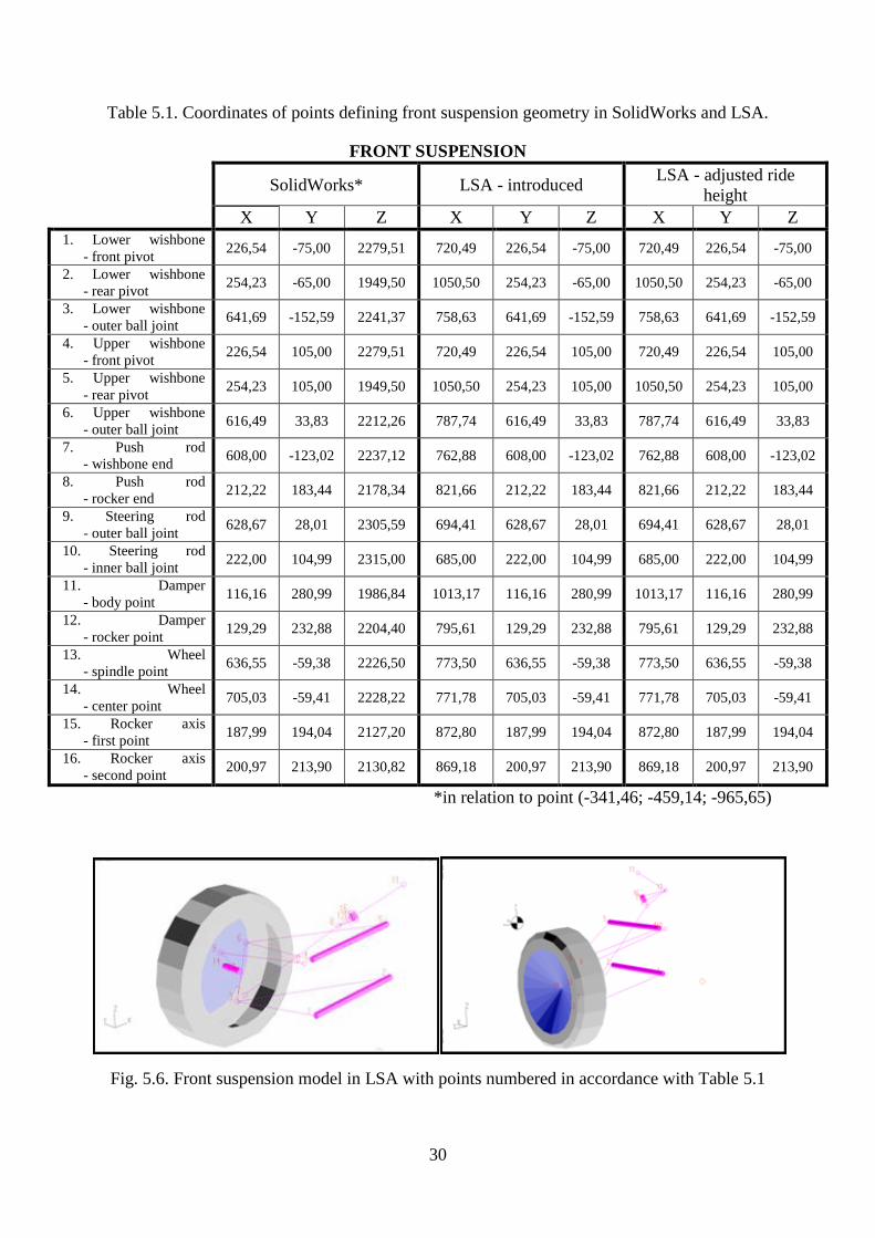
Despite high value of caster, camber gain while turning – around 2° per 15° turning angle - is
lower than suggested in literature - 2° per 10° turning angle (Fig. 6.2). The reason for that
situation is high kingpin inclination, which causes exactly opposite changes in camber. As
camber loss related to body roll (analyzed in following chapter) is very high it can be
concluded that steering related gains will not be able to compensate for them.
34
Fig. 6.2. Camber changes while turning for analyzed vehicle.
6.1.3. Conclusions
First of all it is recommended to decrease kingpin inclination and offset, values of which are
too high in comparison with suggestions from literature and benchmarking. It should be also
underlined that these geometrical parameters have mostly negative influence on vehicle
performance.
As decreasing kingpin inclination increases kingpin offset the only solution for the problem
being analyzed is different packaging of components localized inside the wheel and changes
in upright design in order to move them closer to wheel’s central plane (as far outboard as
possible) or selection of a different wheel.
It was found out that in order to meet budget requirements the design team decided to
purchase wheels and tires designated for quad instead of those normally used in Formula
Student competitions. Later it turned out that the mounting holes of the rims do not match
those on hub’s disc and an additional adapter had to be applied, which resulted in extra
millimeters of kingpin offset. It implies that changing selection of rims would make a
significant and demanded difference.
Remembering that changes in kingpin inclination influence camber gain related to turning,
which should be balanced with camber gain in bump (suggested to be changed in following
part), the final decision about caster angle, that also takes part in camber control, can be made
later (in side view design). It is however suggested to decrease its value below 7° as with
changes that has just been mentioned it should still ensure enough camber gain. Adjusting
caster offset during design is relatively easy as it can be done by offsetting wheel axis in
upright (spindle offset), without influencing other parameters, as it is presented in chapter 3.3.
With some limitations these changes – caster angle and offset - can be also implemented
without changing upright design, because current design includes three different positions of
mounting lower control arm to upright (Fig. 6.3).
-3
-2
-1
0
1
2
3
-20 -15 -10 -5 0 5 10 15 20
turning angle [°]
cam
be
r [°
]
Camber change while turning - ride height
outer inner wheel

35
Fig. 6.3. Bottom view of lower control arm mounted to upright. Three different holes for this
connection are available in the upright.

36
6.2. FRONT VIEW GEOMETRY ANALYSIS
6.2.1. Roll centers
While cornering the car body pivots around roll axis, determined by front and rear roll
centers. As it is preferred that the maximum roll is possibly low the distance between roll axis
and vehicle’s center of gravity should be small, so the rolling torque related to it is low too
(Eq. 3.1). On the other hand that would require roll centers to be placed relatively high.
According to Eq.3.2 both roll angle and roll center height influence growth of difference
between vertical forces on inside and outside wheel in cornering and drop of side forces
generated (chapter 3.5.1). High roll centers also increase jacking forces, causing the
suspension to drop relatively to body (for roll centers above ground or raise for roll centers
below the ground), what limits bump travel related camber compensation. Therefore keeping
roll centers close to the ground is advised.
Table 6.2 present roll center heights for different types of vehicles. The roll center heights of
analyzed vehicle can be also compared to those of other teams taking part in Formula Student
competition. These roll center heights normally do not exceed 50mm [[5[6].
Table 6.2. Roll center heights for different kinds of vehicles (values for front axis in the line
above and for rear below). Race cars (all other than Pkw – passenger car) have roll centers
placed close to the ground – from -26mm (below ground level) to 40mm (above ground
level).[1]
Important part of suspension geometry analysis is also roll centers migration. While rolling it
is required that roll centers follow relatively linear path. If that requirement is not met
unpredictable changes of jacking forces and overturning moment may occur, making handling
more difficult. With bump travel roll centers’ locations should not move significantly
relatively to vehicle’s body’s center of gravity (Fig. 6.4) [1].
Fig. 6.4. Example of acceptable roll center heights changes relatively to ground with bump
travel (f – front, r – rear axis).It can be concluded that roll centers heights do not change their
position relatively to car body significantly.[1]

37
It is also preferred to design rear roll center a little higher than the front one. Typical values of
roll axis inclination are between 0° and 6° [2].
6.2.2. Results analysis – roll centers
In the design of analyzed vehicle roll centers are placed high above the ground comparing to
other vehicles mentioned before. 137,14mm for front axis and 93,08mm for rear. The roll axis
is therefore inclined towards rear of the car (Fig. 6.5).
Roll centers migrating while car body rolls follow a path presented in Fig. 6.6, that should not
cause any unexpected changes to jacking forces or overturning torque. From the Fig. 6.7
however it can be concluded that roll centers change location relatively to body’s center of
gravity, which implies that changes in overturning torque occur.
Fig. 6.5. Roll axis in side view. Front roll center (left) is placed higher above the ground than
the rear.
Fig. 6.6. Roll centers’ migration with roll of the vehicle’s body.
0
20
40
60
80
100
120
140
160
-200 -150 -100 -50 0 50 100 150 200 Y [mm]
Z [m
m]
Roll centers migration in YZ plane; -3° to 3° body roll
Front Rear

38
Fig. 6.7. Roll centers height change with bump travel. As roll centers’ height changes faster
than bump travel it can be concluded that their location changes relatively to body’s center of
gravity.
6.2.3. Camber gain
The allowable values of camber angle depend on the tire requirements, the power to weight
ratio, usage on driven or non-driven axis and the aerodynamic properties. This however can
be controlled by adjusting static camber.
The camber angle should be changing with bump travel, growing to the negative side. That
tendency compensates for changes related to roll movements of the body. Moreover as the
outer wheels while cornering carry more load and therefore their tires are submitted to
significant side deformations, the increasing camber is supposed to compensate those
deformations too, ensuring better contact conditions between the tire and road. Analyzing
diagrams form Fig. 3.22 it can be concluded that adding negative camber to strongly loaded
tire results in very beneficial grow of cornering force. If there is no exact data for the tires
chosen available, it can be assumed that camber values below 5° are the optimum [3].
The inner wheel, being in rebound, should remain normal to the road (camber=0°) or gain low
positive value. Higher values of camber, positive or negative, could cause side of the tire to be
lifted, which would decrease side forces generated.
Example curve of camber changes in bump travel is presented in Fig. 6.8.
Taking into consideration advices from literature and benchmarking the following design
goals for camber can be formulated:
Camber change should remain less than 1° per 1° roll angle of the car body and about
25 mm wheel travel [1]. Can be 0,2°-0,3° per 1° roll for front axis and 0,5°-0,8° per 1°
roll for rear axis, that is not affected by steer related camber gain [6].
It is preferred for the wheel in rebound not to change camber and remain 0° or reach
low positive values [1].
-60
-40
-20
0
20
40
60
-40 -30 -20 -10 0 10 20 30 40
bump travel [mm]
roll
cen
ter
he
igh
t [m
m]
Roll centers height change with bump travel
Front Rear

39
Due to different conditions of particular competitions static camber has to be easily
adjustable from 0° to 4°.
Fig. 6.8. Examples of acceptable relation between camber gain and bump travel
6.2.4. Results analysis – camber gain
The following diagrams (Fig. 6.9 - Fig. 6.11) present analyzed vehicle’s suspension
properties, that can be used to verify whether the design goals pointed in previous chapter are
met: Camber gain with bump travel for front (Fig. 6.9) and rear axis (Fig. 6.10) and camber
loss for body roll (Fig. 6.11).
It can be noticed, that the camber gain with bump travel for front axis is very low (0,06° per
30mm bump travel from ride height) while for the rear axis camber grows slightly to positive
values (camber loss). As a result camber compensation related to bump travel practically
cannot be observed in body roll. In Fig. 6.11, presenting camber changes with body roll the
plotted lines stand for linear relation between camber values and angle of body roll with ~1°
camber loss per 1° body roll. This situation is even more disadvantageous for rear axis, which
does not have compensating camber changes related to steering analyzed in following chapter.
Fig. 6.9. Camber gain with bump travel for front axis. Camber values grow towards negative
values with bump travel, gaining however only 0,06° per 30mm bump travel from ride height.
-0,06
-0,04
-0,02
0
0,02
0,04
0,06
-40 -30 -20 -10 0 10 20 30 40 bump travel
[mm]
cam
be
r [°
]
Camber gain with bump travel - front axis
compressiorebound
40
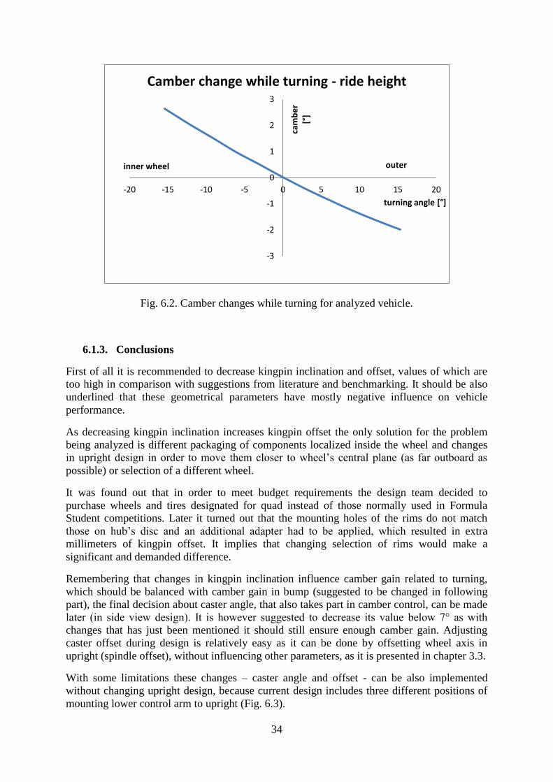
Fig. 6.10. Camber gain with bump travel for rear axis. Camber values slightly grow towards
positive values –camber loss.
Fig. 6.11. Camber loss with body roll for front and rear axis. Camber changes are practically
equal to angle of body roll - ~1° camber loss per 1° body roll.
6.2.5. Track width change and bump steering
Another characteristic related to front view geometry analysis that should be taken into
consideration is track width change with bump travel. As it can laterally disturb the car and
increase rolling resistance, these changes should be diminished. According to [2] track change
should not be more than 20mm (for street cars).
Similar effects on the car can be also caused by toe angle changes related to bump travel and
these should be as low as possible too. Despite being related rather to steering system
geometry, this phenomenon is analyzed in this report for the reason of being easily analyzed
with LSA and because of suspension travel being one of the causes of these changes.
-0,7
-0,6
-0,5
-0,4
-0,3
-0,2
-0,1
0
-40 -30 -20 -10 0 10 20 30 40
bump travel [mm]
cam
be
r [°
]
Camber gain with bump travel - rear axis
compressiorebound
-4
-3
-2
-1
0
1
2
3
4
-4 -3 -2 -1 0 1 2 3 4
roll [°]
cam
be
r [°
]
Camber loss with body roll
front axis rear axis
outer inner wheel

41
Especially bad influence on the car behavior in the turn is the one of nonlinear toe angle
(Fig. 6.14). Bump travel curve, while linear, directed to understeer (Fig. 6.13) in roll can be
even favorable as they imply compensation to compliance effects in the steering system.
Examples of acceptable characteristics of track width and toe angle changes with bump travel
are presented on Fig. 6.12 and Fig. 6.15 respectively.
Fig. 6.12. Example of acceptable track width change with bump travel.[1]
Fig. 6.13. Example of wheel that tends to toe-out with jounce and toe-in in rebound. The
curve suggest correct length of the steering rod (linear relation), but incorrect position of ball
joints – inner too low, or outer too high. [3]

42
Fig. 6.14. Example of wheel that tends to toe-out both in jounce and rebound, passing through
initial position in ride height. The curve suggest that the ball joints of the steering rod are
placed in the correct height, but it is too short. [3]
Fig. 6.15. Example of acceptable toe angle change with bump travel. [1]
6.2.6. Results analysis - track width change and bump steering
Both diagrams obtained from analysis in LSA present that changes of (half) track width
(Fig. 6.16) and toe angle (Fig. 6.17) are more rapid than those presented as an example above.
With 30mm rise of suspension width track grows over 4mm for rear axis and 8mm for front
(half track over 2mm and 4mm respectively). Literature suggests however even 30mm scrub
change as acceptable, but for street cars (and with much longer bump travel typical for that
kind of cars), while example typical for race cars suggests only 3mm growth. Toe angle
changes even 0,15° for front axis, comparing to less than 0,08° suggested before. Only toe
angle change for rear axis stays within accepted boundaries.
As the relation between steer angle and bump travel is almost linear, it can be concluded that
it is more important to apply changes in steering rod’s location rather than its length.

43
Fig. 6.16. Half track change with bump travel for analyzed vehicle.
Fig. 6.17. Toe angle change with bump travel for analyzed vehicle.
6.2.7. Conclusions
It can be concluded that the suspension does not meet all of the design goals set, related to
front view geometry. It is advised to manipulate control arms configuration in order to obtain
higher camber gains with bump travel compensating for camber loss related to body roll. The
desired relation should be non linear with more rapid changes for compression than for
rebound, resulting in maintaining camber of inner wheel low over 0° and outer wheel growing
to negative values while roll.
These changes of camber value should be a little bigger for rear axis while those for front axis
must be balanced with changes related to caster and kingpin inclination analyzed in previous
chapter.
-8
-6
-4
-2
0
2
4
6
-40 -30 -20 -10 0 10 20 30 40 bump travel
[mm]
hal
f tr
ack
chan
ge
[mm
]
Half track change with bump travel
Front Rear
compression
rebound
-0,2
-0,15
-0,1
-0,05
0
0,05
0,1
0,15
-40 -30 -20 -10 0 10 20 30 40 bump travel
[mm]
toe
an
gle
ch
ange
[°
] Toe angle change with bump travel
Front Rear
compression
rebound

44
The above can be obtained in the following process according to literature [3]
Set demanded values for camber gain for front and rear axis. For example
0,3° camber gain relatively to ground per 1° body roll for front axis and 0,7° for rear
axis.
Calculate fvsa length for ride height according to Eq. 3.3, getting, following the
example camber gain values,
(Eq. 6.1)
for front axis and
(Eq. 6.2)
for rear axis.
After deciding on roll center heights (advices in following paragraph of this chapter),
which together with fvsa length determine instant centers for front view geometry,
design lower control arm as long as packaging restraints allow (ball joints on upright
should be already placed) and manipulate upper control arm’s length until demanded
relation between camber and roll is obtained. LSA should be a really helpful tool in
that case as it can automatically plot diagram of this relation in real time, while
changes are being made.
Roll centers should be placed lower. Their height, according to benchmarking, shouldn’t be
more than 40mm with lower value in the front. As their height (together with fvsa) is first to
be decided in the design process, this change is very easy to make.
Lowering roll centers and what follows moving instant centers closer to ground level
according to Fig. 3.4 will result in favorable decrease in track width changes too.
When it comes to the phenomenon of bump steering (toe angle change with bump travel)
a slight change of steering rack location is suggested. Due to compliance effects however it is
better to move it down, close to lower control arm as in Fig. 4.1 (placing it behind the axle
line is difficult because of packaging problems caused by required in competition rules empty
area template – red box in Fig. 6.18). The differences in stiffness of mounting the rack and the
control arms may cause steering angle changes under side forces while cornering. Ensuring
that the steering rack is located in indicated areas it will be more likely to obtain understeering
in this situation rather than oversteering, which is safer, taking into consideration vehicle
stability.

45
Fig. 6.18. Single Cardan’s coupling and the steering rack located in front of and above front
axis. Red extrusion is the empty area template required in the competition.
In order to obtain these changes a double Cardan’s coupling should be applied to solve
packaging issues around empty area template. Additional benefit would be also elimination of
angular velocity pulsation, which appears on passive shaft when a single coupling of this type
is used.

46
6.3.SIDE VIEW GEOMETRY ANALYSIS
6.3.1. Anti features
The advantages of high values of anti features is decreasing vehicle’s pitch while accelerating
and braking. Designing full anti features however is not usual or even impossible because of
several reasons. Full anti features are subjectively undesirable and the requirements for
achieving them may conflict with those for good handling or braking.
According to source [2] the typical values for anti-squat are between 60% to 80% and anti-
dive 60% to 70% (according to [4] seldom more than 50%). Other example values are
presented in Fig. 6.19. 40% to 50% for anti-squat and 40% to 60% for anti-dive.
It is important to remember that as anti features are related to instant centers of rotation their
values change with suspension travel and should lay within desired limits for all the wheel
position range.
Fig. 6.19. Example acceptable values of anti-dive (left) and anti-squat in bump travel [1].
6.3.2. Results analysis - anti features
For analyzed formula student vehicle anti-dive values for front and rear axle stay between
33% and around 35% within whole bump travel (Fig. 6.20). These values are lower than any
of the sources advices.
The value of anti-squat (Fig. 6.21) (only for rear axle – front axle is non-driven and does not
produce anti-squat forces) change from almost 50% in rebound to less than 40% in
compression and can be considered correct according to some of the sources.

47
Fig. 6.20. Analyzed vehicle’s anti-dive values for front and rear axle changing with bump
travel.
Fig. 6.21. Analyzed vehicle’s anti-squat value (rear axle) changing with bump travel
6.3.3. Conclusions
It is advised to increase values of anti features of the analyzed vehicle, especially anti-dive.
The design process presented in the beginning of this work suggest starting the side view
geometry for front axle with following steps:
Deciding on desired anti-dive value. With given braking force distribution,
% front braking, center of gravity height, h and wheelbase, l, angle ϕ (tanϕ) can
be calculated according to Eq. 3.4. For 50% anti-dive and 60% of braking force
on front axis:
(Eq. 6.3)
(Eq. 6.4)
32,5
33
33,5
34
34,5
35
35,5
-40 -30 -20 -10 0 10 20 30 40
bump travel [mm]
anti
-div
e
[%]
Anti-dive with bump travel
Front Rear
compression rebound
0
10
20
30
40
50
60
-40 -30 -20 -10 0 10 20 30 40
bump travel [mm]
anti
-sq
uat
[%
]
Anti-squat with bump travel - rear axis
compression rebound

48
Deciding on shortest practical svsa in order to locate IC on the line determined
by angle ϕ (Fig. 4.3).
For rear axis a compromise between anti-dive and anti-squat will be required as after locating
side view IC for rear suspension, their values will be calculated according to different force
diagrams (look Fig. 3.24 for anit-dive and Fig. 3.25 for anti-aquat) and equations (Eq. 3.5 for
anti-dive and Eq. 3.6 for anti-squat).

49
7. FRAME PERFORMANCE TESTS AND GOALS
According to [7] the loads that a vehicle’s frame is subjected to during normal exploitation
can be simulated with four different tests that all together, if passed with positive result
guarantee it’s correct performance. These tests are:
Longitudinal torsion
Vertical bending
Lateral bending
Horizontal lozenging
Longitudinal torsion takes place when two oppositely directed forces act on corners of the car,
generating torque along the longitudinal axis of the car. Vertical bending is caused by weight
of passenger and car’s components installed on the chassis. The magnitude of these forces can
by increased in comparison to static situation, when vertical accelerations appear. Lateral
bending appears when the car is subjected to side forces related for example to side wind or
centrifugal acceleration while cornering. Horizontal lozenging takes place when differences in
longitudinal forces appear between tires on opposite sides of the car, making the chassis
distort into parallelogram shape. These four loading schemes can also happen simultaneously.
Fig. 7.1 Chassis deformation modes [7]
Usually, and in this paper too, the attention is focused on the test of longitudinal torsion and
the frame’s performance in it is considered the primary factor when the structure is assessed.
This is caused by the fact that frame’s deformations under torsional loads can influence
handling performance, by changing roll angles of axis and load distribution on tires [8].
For this kind of test design’s performance can be expressed as torsional stiffness in Nm per
degree, which is torsional torque related to twist angle that it causes. On this basis a design
goal can be set. Although there is no specific value that can be considered an optimal one and

50
the only objective way to asses overall frame’s performance are track tests, the design teams
usually assume that the chassis’s stiffness should be one order magnitude greater than either
spring, wheel or tire rate [7]. If a theoretical situation, when all the chassis elements except for
shock absorbers (springs and dampers) are perfectly stiff (frame, control arms, push rods,…
and all the joints and bearings) is imagined, the goal can be also set as follows: The chassis
torsional stiffness must constitute 90% of the perfectly rigid case [7]. The last approach was
applied in this paper and all the required calculations are performed in following part.
In addition to the usual analysis of the frame, some more attention will be paid to its behavior
around joints of suspension’s control arms too. Their location, in some distance from nearest
frame’s nodes, could be considered a disadvantage of a design, that increases suspension
system’s compliance. It can change critical suspension’s point’s (the same as were introduced
to LSA model) relative location and influence steering performance because of it. Strategic
location of suspension support points is also a target for a rigid chassis design [9].

51
8. RIGID CHASSIS CASE
To calculate the chassis torsional stiffness for a theoretical, perfectly rigid frame a simple
mathematical model presented in Fig. 8.1 will be used. It consists of frame and four springs
placed in its corners, that represent the suspension. Three of them are fixed to the ground. On
the fourth one there is a vertical force acting upwards. That model is analogical to a situation
when three wheels of a car are located on a flat, horizontal surface and the fourth is on a
bump. The forces that keep the three wheels at the ground are the loads coming from the car’s
weight [7].
Fig. 8.1 Mathematical model for torsional stiffness calculations for rigid chassis case
Under the force the system will change its position to presented in Fig. 8.2. The rear left and
front right springs will rebound and the other two will be compressed. Moreover the spring
that is not fixed to the ground will move upwards. For this calculations it will be assumed that
only vertical deflections and translations appear.
The twist angle of chassis in this situation, that will be needed to calculate torsional stiffness,
is the angle that the line connecting bottom ends of the front springs creates with the ground.
It is the same angle that this line creates with analogical line drawn for the rear springs, whose
ends remained on the ground. If the system is presented with the frame instead of the ground
as reference, as in Fig. 8.3, this angle can be easily related to springs vertical deformations.
Fig. 8.2 Systems position under the force acting with the ground as reference

52
Fig. 8.3 Systems position under the force acting with the frame as reference
This angle will be therefore the sum of inclinations of the lines connecting bottom ends of
lines in front and rear relatively to their initial positions and can be calculated as follows:
Eq. 8.1
Eq. 8.2
Eq. 8.3
where: ϕ – chassis twist angle
ϕF, ϕR – inclination of front/rear line connecting bottom ends of springs
dy – vertical deflection of front/rear right/left spring
tF, tR – front/rear track
Solving the free body diagram of the system for a force of 1000N acting on one of the front
springs gives the reaction force of 1000N on the other front spring and 1020N at rear springs.
The torque T acting on the frame is:
Eq. 8.4
Springs in this model represent wheel rates of the vehicle. To calculate the deflections then
the spring stiffness has to be multiplied by installation rate squared, that can be read from
LSA data. The program however gives the values as spring ratio, that have to be inverted to
be used in Eq. 8.7 and Eq. 8.8. Fig. 8.4 presents on a simple model how the installation rate
determines relations of both forces and displacements/deflections, what makes it necessary to
square it.
Fig. 8.4 Force and displacement relations between wheel and spring

53
The simplified model depicts a suspension with single wishbone and a spring attached in half
of its length. From the equilibrium of moments it can be concluded that the force acting on the
spring is twice the force at the contact patch of the tire. From geometrical relations the
spring’s deflection equals half of the tire’s vertical translation as long as small angles are
considered. The value given by LSA takes into consideration, except for rocker’s ratio, also
corrections related to angles which the spring and push rod create with it. As this angles
change constantly with bump travel, rounded values for ride height were used in calculations.
The spring stiffness is given on them by producer in pounds per inch, so in N/mm they are:
Eq. 8.5
For front and
Eq. 8.6
for rear.
The wheel rates kF for front and kR for rear are then:
Eq. 8.7
Eq. 8.8
The deflections of the model’s springs or in other words wheels’ vertical displacements are
therefore:
Eq. 8.9
Eq. 8.10
The twist angle can be now calculated according to Eq. 8.1, Eq. 8.2 and Eq. 8.3.
Eq. 8.11
And with torque calculated in Eq. 8.4 gives the torsional stiffness
Eq. 8.12
For the case with compliant chassis the torque T will cause twist angle ϕ related to shock
absorbers’ deflections and additional twist in chassis, related to its limited stiffness, that will
be determined in virtual and laboratory tests. Dividing the torque by sum of these angles will
give the compliant case’s torsional stiffness. These deflections are therefore treated as for
springs in series, so the final stiffness can also be calculated as follows:
Eq. 8.13

54
Fig. 8.5 presents a mathematical model with compliant chassis and results of calculations
done by far. There is a torsional spring placed in the middle of the chassis, that subjected to
torque T lets the chassis twist by angle φchassis along its longitudinal axis.
Fig. 8.5 Mathematical model of case with compliant chassis
If torsional stiffness of rigid chassis is known and the goal for compliant frame is set as 90%
of it, then the demanded chassis stiffness can be calculated on basis of Eq. 6.14.
Eq. 8.14
Eq. 8.15
This value, if compared to Table 10.5, turns out to be very high. None of the frames
mentioned there for benchmarking could meet the goal of 90% (452,47 Nm/°) of the rigid case
stiffness with that suspension’s torsional stiffness value. The most rigid frame of 2711,64Nm/°
would result with barely 84%. Note, that because of character of Eq. 6.13 this percentage is an
asymptotic function of chassis stiffness and with values getting closer to 90% a substantial
growth in chassis stiffness is needed for it to grow another percentage point (Fig. 8.6). That
means that springs chosen for the suspension are very stiff and revision of their selection
process is recommended. That has to be taken into consideration when results of the tests are
analyzed.
rear right:
F=1020N
kR=66,9N/mm
dyRR=-15,25mm
rear left:
F=-1020N
kR=66,9N/mm
dyRL=15,25mm
front right:
F=-1000N
kF=78,5N/mm
dyFR=12,74mm
front left:
F=1000N
kF=78,5N/mm
dyFR=-12,74mm
chassis:
T=1282Nm
Kchassis=4524,75Nm/°
φchassis =0,28°
front axis:
φF =1,14°
rear axis:
φR =1,41°

55
Fig. 8.6 Relation between chassis and full vehicle torsional stiffness for suspension torsional
stiffness K=502,75 Nm/°
K = 502,75
K= 452,47
0
100
200
300
400
500
600
0 2000 4000 6000 8000 10000 12000
Ve
hic
le t
ors
ion
al s
tiff
ne
ss [
Nm
/°]
Chassis torsional stiffness [Nm/°]

56
9. TESTS PROCEEDINGS
The following part of the report contains description of methodologies and results of several
virtual and experimental tests. To make the flow of them and relations between them clear,
they are presented in Fig. 9.1.
Although in all the tests the structure is in longitudinal torsion, there are important differences
between one another. Except for obvious division between virtual and experimental tests we
can differentiate tests run for only the frame, without suspension, and tests of full chassis
assembly. Except for determining the torsional stiffness in these tests, which was the main
goal, also the values of stress were checked. Therefore stiffness and stress tests can be
distinguished too.
Finite Elements Analysis Experimental Tests
Frame:
-normal boundary conditions
torsional stiffness
stress
-as in experimental test
torsional stiffness
stress
Frame:
torsional stiffness
stress
-others
Chassis
torsional stiffness
stress
Chassis:
torsional stiffness
stress
Fig. 9.1 Tests proceedings
The experimental tests were run to verify and validate the virtual ones. If considerable
discrepancies appeared, that would mean the model does not represent the reality properly, of
course as long as no mistakes are made in experimental tests. The model however is always
some kind of simplification of reality and reaching exactly the same results as in experiments
is not possible. Reaching close results in both virtual and experimental approach then will
validate the virtual one and make it possible to further use it, for example to predict stiffness
gains due to improvements proposed. It will also show how accurate the results that the model
delivers are and what change can be expected from the real chassis.
What was already mentioned and will be explained more profoundly later, the car was still
undergoing adjustments in the period when the experiments were run. The current state of the
vehicle made it impossible to set boundary conditions, fixtures, the same way they were
planned for software analysis. For that reason additional FEM analysis that copied the
boundary conditions possible for test in laboratory were run. They could be then directly
compared to practical experiments. The changes regarded mounting the engine and placing
the supports in the rear of the car.
As in literature and practical use many methods of fixing the frame, that are different than the
one chosen here, are common, they will also be considered. Minor attention however will be
paid to them.

57
10. FINITE ELEMENTS ANALYSIS
10.1 MODEL CREATION
The virtual SolidWorks manufacturing model, previously prepared by design team, was used
to prepare model for simulations. It required first of all introducing all the changes between
the model and the welded frame that appeared during manufacturing as a result of design
teams decisions. The example changes appeared in side of the frame, next to the seat and are
presented in Fig. 10.1 together with the original model of the frame delivered for virtual tests.
Fig. 10.1 Original frame model and example change made during manufacturing
The manufacturing model turned out not to be well prepared for virtual tests. In spite of much
time being spent on adjusting it for this purpose, problems with meshing kept occurring.
Because of it, the decision was made to make a new model, dedicated specifically for the
analysis. Therefore the model initially delivered, welded frame check for differences and few
measurements were the basis for creating a new model. It used the technique of three-
dimensional sketch which is the basis for locating in space structural members of defined
cross-sections.
Fig. 10.2 3D sketch for the simulations model
Basing on source papers [7, 10] and SolidWorks online resources [11] dedicated for Formula
SAE, it was decided that beam elements model will provide results accurate enough. Most of
the elements were therefore treated as beams, transferring forces and moments in all

58
directions, except for suspension elements, that were treated as trusses, transferring only
longitudinal forces. That very easily simulated ball joint connections of control arms. The full
mesh is presented in Fig. 10.4. The trusses can be distinguished from the beams, as they are
single, long elements not further divided into smaller ones.
At that point it was necessary to decide what kind of elements, except for the frame itself,
should be considered in the simulations, as they could influence the results and what kind of
simplifications can be applied in order for the program to be able to perform the calculations.
It is worth mentioning, that frame model should be subjected to virtual torsional stiffness test
in the phase of design, between following iterations. For that reason creating a simple model,
that goes through the program’s calculations fast can make it easy to test and assess any
adjustments introduced and save time. Following the same approach in this work will provide
results that can be a point of reference when a frame for next season is designed. As the
laboratory tests will be performed too, it will reveal how close to the actual, real chassis
torsional stiffness they are too.
Mountings of other systems were not included in the model, neither were thin plates below
the frame and behind the driver’s back or side safety structures. Engine however, together
with gearbox in this case, considerably increases frame’s stiffness and in a good, lightweight
design should be considered a structural element [10]. Also the front plate was considered in
the analysis, as it prevents the front hoop of the frame from deforming.
In order to keep the model consist exclusively of beam elements, those two parts were
simplified and replaced with simple, stiff beam structures, that increased the frames’ rigidity
in specific areas [7, 10]. The chassis’ simplified version designated for analysis, together with
beam structures representing engine, gearbox and front plate can be seen in Fig. 10.3.
Fig. 10.3 Chassis model prepared for tests and beam structure replacing engine and gearbox
Another simplification regarded removing rocker from suspension and connecting the push
rods directly to the frame. That will change loads distribution in this area. It should not
however significantly change the final result of torsional stiffness.
It can be noticed that beams in the model prepared for tests are not trimmed in the connections
with one another and intersect. It was decided to do so, because of the algorithm that the
software follows to create mesh. The initial three-dimensional model is a base for creating set
of nodes (Fig. 10.4), which the beam elements are extended between. Such a limited treatment
of pipes’ connections gave better final result.
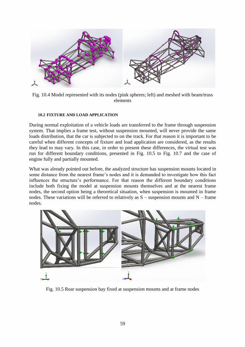
59
Fig. 10.4 Model represented with its nodes (pink spheres; left) and meshed with beam/truss
elements
10.2 FIXTURE AND LOAD APPLICATION
During normal exploitation of a vehicle loads are transferred to the frame through suspension
system. That implies a frame test, without suspension mounted, will never provide the same
loads distribution, that the car is subjected to on the track. For that reason it is important to be
careful when different concepts of fixture and load application are considered, as the results
they lead to may vary. In this case, in order to present these differences, the virtual test was
run for different boundary conditions, presented in Fig. 10.5 to Fig. 10.7 and the case of
engine fully and partially mounted.
What was already pointed out before, the analyzed structure has suspension mounts located in
some distance from the nearest frame’s nodes and it is demanded to investigate how this fact
influences the structure’s performance. For that reason the different boundary conditions
include both fixing the model at suspension mounts themselves and at the nearest frame
nodes, the second option being a theoretical situation, when suspension is mounted in frame
nodes. These variations will be referred to relatively as S – suspension mounts and N – frame
nodes.
Fig. 10.5 Rear suspension bay fixed at suspension mounts and at frame nodes

60
Fig. 10.6 Single plane of rear suspension bay fixed at suspension mounts and at frame nodes
Fig. 10.7 Single line of rear suspension bay fixed at suspension mounts and at frame nodes
The concept referred to as “rear bay” assumes that all the mounts of rear control arms are
totally fixed for translations, with free rotations and can be often found in other papers. This
however assumes, that suspension mounts do not change their location in relation one to
another, which does not have to be true, especially in the case, when no proper triangulation is
provided in the area of suspension mounts. On the other hand suspension, if mounted, also
provides some support to suspension mounts, when compared to situation, when only the rear
mounts of rear bay are supported (referred to as “single plane of rear bay”) and the other
mounts are free to translate.
It also should be assumed that top and bottom suspension mounts can move relatively. Even
with stiff pipes installed instead of shock absorbers, the suspension is still a truss structure and
changes its position without generating any moment counteracting frame deformations.
Another fixture concept then, with frame fixed at the bottom rear of rear suspension bay,
locks dislocation of only two points and allows all the others to move. Running test with these
boundary conditions will include rear suspension bay’s compliance effects in the results. It is
also the closest to the conditions that can be provided for the laboratory test, which will be
explained in following part of this paper. For this reason it was chosen for more profound
analysis.

61
It can be concluded that the real value of torsional stiffness, the one, that characterizes chassis
on the racing track, lays somewhere between the limits set with the values gained from the
tests described.
No matter which of the fixture concepts is considered, it should be later verified, being
compared to results from full chassis test.
Analogical considerations could be conducted for force and fixture application in the front of
the car. For having a clear way of calculating the torque however, and what follows
determining a value of torsional stiffness unequivocally, the structure was introduced in
torsion with a single force and fixture in vertical and side directions. They were applied either
on the bottom front line of front suspension bay or, for the simulation of test run in workshop,
in the further front bottom pipe (Fig. 10.8).
Fig. 10.8 Fixture and load application in front of the car
For full chassis assembly the tests were run with bottoms of three uprights fixed for
translations. Rear right in all three directions, rear left for vertical direction and front right for
side and vertical direction. The force was applied downwards at the fourth upright (Fig. 10.9).
Fig. 10.9 Fixture and load application for full chassis assembly test

62
10.3 VIRTUAL FRAME TEST
Table 10.1 presents results of the virtual tests for all the boundary conditions concepts, while
Fig. 10.10 and Fig. 10.11 depict vertical dislocations for two most important cases: single line
fixed with mounted engine, which was considered the correct way of running the test and the
case with the same boundary conditions as in experimental test.
Table 10.1 Virtual frame tests results
engine fully mounted engine NOT fully mounted
fixture force [N] L [mm] Torque [Nm] dy [mm] angle [°] K [Nm/°] dy [mm] angle [°] K [Nm/°]
suspension bay N
1000 394 394
0,73 0,11 3737,07 0,75 0,11 3616,36
suspension bay S 0,81 0,12 3352,78 0,84 0,12 3242,82
single plane of
suspension bay N 1,00 0,14 2717,26 1,10 0,16 2458,60
single plane of
suspension bay S 1,11 0,16 2438,69 1,20 0,17 2265,37
single line of
suspension bay 1,369 0,20 1979,09 1,63 0,24 1660,16
as in lab test 364 364 1,016 0,16 2276,07 1,06 0,17 2191,94
Fig. 10.10 Vertical dislocations for single line fixed and engine fully mounted

63
Fig. 10.11 Vertical dislocations for experimental test’s boundary conditions
Using virtual tests it was possible to easily calculate torsion angle not only for a frame as a
whole, but also for specific compartments along Z axis, which the frame is divided into by
vertical pipes. Dislocations dy1 and dy2 along Y axis were read for two points in the end of
each compartment. Knowing the distance x between them the angle φ was calculated with
simple trigonometry relations. The angle was calculated for top and bottom line as presented
in Fig. 10.12. The results are gathered in Table 10.2. The twist angle analysis was conducted
for the fixtures in one line of rear bay.
Table 10.2 Twist angle analysis for virtual frame test (single line of suspension bay fixed)
z [mm] -927 -732 -473 0 862 1016 1349 1534
x [mm] 120 260 354 620 476 448 392 362
upper
line
engine fully
mounted
dy1 [mm] 0,032 -0,005 -0,251 -0,711 -1,129 -1,180 -1,301 -1,352
dy2 [mm] 0,100 0,004 0,129 0,280 0,139 0,089 -0,006 -0,076
φ [°] 0,032 0,002 0,062 0,092 0,153 0,162 0,189 0,202
bottom
line
dy1 [mm] 0,033 0,000 -0,252 -0,708 -1,129 -1,186 -1,307 -1,350
dy2 [mm] 0,100 0,000 0,131 0,278 0,140 0,093 0,000 -0,077
φ [°] 0,032 0,000 0,062 0,091 0,153 0,164 0,191 0,201
upper
line
engine NOT
fully mounted
dy1 [mm] 0,051 -0,008 -0,399 -1,054 -1,470 -1,521 -1,643 -1,693
dy2 [mm] 0,086 0,008 0,226 0,482 0,211 0,137 -0,006 -0,104
φ [°] 0,017 0,004 0,101 0,142 0,202 0,212 0,239 0,252
bottom
line
dy1 [mm] 0,051 0,000 -0,403 -1,055 -1,472 -1,529 -1,650 -1,694
dy2 [mm] 0,085 0,000 0,229 0,479 0,212 0,142 0,000 -0,104
φ [°] 0,016 0,000 0,102 0,142 0,203 0,214 0,241 0,252

64
Fig. 10.12 Twist angle value along longitudinal axis of the vehicle in frame test
From analysis of the results presented above following conclusions can be drawn.
Results of tests run with different fixture concepts are significantly different. They vary from
1979,09 Nm/° to 3737,07 Nm/° for the case with mounted engine and from 1660,16 Nm/° to
3616,36 Nm/° with engine partially mounted. Moreover the compartment of the rear bay,
where the load distribution is directly influenced by these concepts appears to be critical, as it
can be seen in Fig. 10.12. To assess which of the fixture concepts considered is the most
accurate, the results will be later verified with full chassis assembly test.
Fixing the frame at its nodes instead of the suspension mounts also changes the resulting
torsional stiffness substantially. A theoretical case in which the suspension is mounted in the
nodes of the frame in comparison to mounting it outside the nodes increases the stiffness for
engine mounted from 3352,78 Nm/° to 3737,07 Nm/° (11,5%) for whole bay fixed, and from
2438,69 Nm/° to 2717,26 Nm/° (11,4%) for single plane fixed. For engine partially mounted
the stiffness increases from 3242,82 Nm/° to 3616,36 Nm/° (11,5%) and from 2265,37 Nm/°
to 2458,60 Nm/° (8,5%) respectively. That indicates also a problem other than just loss of
torsional stiffness. Compliance at control arms’ mounts, which appears in this case, results in
changes of relative location of suspension points and in its behavior different than designed.
Special attention should be paid to ensuring rigidity in that area. Deformation of left rear
pipes which the control arms are mounted to can be seen in Fig. 10.13.
0,000
0,050
0,100
0,150
0,200
0,250
-1000 -500 0 500 1000 1500
bottom / not mounted
upper / not mounted
bottom / mounted
upper / mounted

65
Fig. 10.13 Pipes deformation under suspension support. Displacement along X (sideways; on
the left) and Z (fore/aft; on the right) axis.
Comparing the torsional stiffness for the cases with fully and partially mounted engine a
growth of 3,3% to even 19,2% can be observed with higher values for less restrained cases.
The stiffness is improved mostly in the suspension bay (Fig. 10.12) and to some extent in the
following compartment, where the slope drops from 8,36 x 10⁵ to 6,14 x 10
5 for the bottom
surface of frame. The less significant influence on torsional stiffness in that compartment is
caused by the fact, that it already has better triangulation than the suspension bay and did not
cause so much deflection even without the engine. Engine mounts in this compartment
however are not located in frame nodes and pipes there bend easily. Better use of engine for
chassis’ stiffness could be expected if the mounts of engine were properly triangulated.
The points of maximum stress (axial and bending) in the structure were indicated at
connections of beams of the floor in the front of the vehicle and reached the maximum of
almost 33 MPa. Due to the fact that the metal sheet already welded to the floor of the frame
tested in the laboratory could to some extent change the stress values other points of high
stress were chosen to compare results of virtual and laboratory test. These points, at the hoop
in front of the driver, are presented in Fig. 10.14 and they reach values of 22,57 MPa and
18,66 MPa.
It is necessary to explain, that in the figure the values indicated refer to the maximum stress in
the beam elements pointed. The exact location of the maximum stress within them can be
found with the help of the legend for colors.
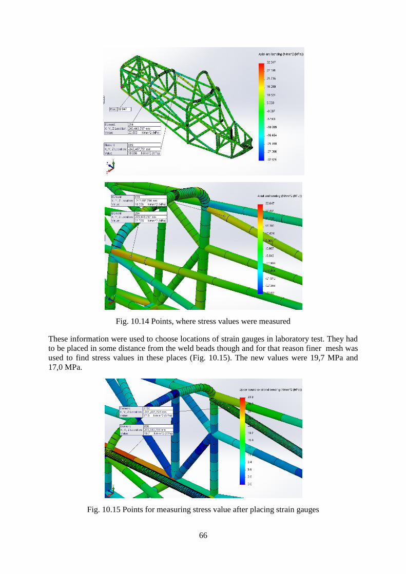
66
Fig. 10.14 Points, where stress values were measured
These information were used to choose locations of strain gauges in laboratory test. They had
to be placed in some distance from the weld beads though and for that reason finer mesh was
used to find stress values in these places (Fig. 10.15). The new values were 19,7 MPa and
17,0 MPa.
Fig. 10.15 Points for measuring stress value after placing strain gauges

67
10.4 VIRTUAL CHASSIS TEST
The results for full chassis assembly, presented in Table 10.4 are 1960,3 Nm/° for engine fully
mounted and 1850,1 Nm/° for engine partially mounted. That is a decrease comparing to most
results of frame test, caused by additional deflection in suspension elements. For a single line
fixed in the rear bay however the frame test results were even lower and for that reason should
be assessed as irrelevant to describe frame behavior in real working conditions. Omitting
them, the case with fixtures in frame nodes, which was purely theoretical and the virtual
simulation of laboratory test, which excluded the rear bay completely, the frame torsional
stiffness lays between 2265,37 Nm/° and 3352,78Nm/° in virtual tests.
The screens from SolidWorks presenting vertical translations in the chassis are presented in
Fig. 10.16 and Fig. 10.17
Table.10.4 Virtual chassis test results
Engine fully mounted engine NOT fully mounted
force [N] L [mm] torque [Nm] d [mm] angle [°] K [Nm/°] d [mm] angle [°] K [Nm/°]
1000 1266 1266 14,27 0,646 1960,29 15,12 0,684 1850,09
Fig. 10.16 Vertical translation diagram for fully mounted engine case

68
Fig. 10.17 Vertical translation diagram for partially mounted engine case
These results used in Eq. 6.11 show that the goal of 90% of torsional stiffness of theoretical
rigid case is not met and the chassis stiffness is barely 79,62% of it. Remembering the relation
between chassis stiffness and overall stiffness of the car from Eq. 8.13 and Fig. 8.6 and value
of 4524,75Nm/° that is needed to meet the goal, the chassis stiffness would have to grow 2,3
times. That result is unsatisfying and means that whenever the vehicle is subjected to torsion
the suspension’s work will be substantially affected.
On the other hand if the result is compared to stiffness of other example Formula Student
designs (Table 10.5) it is not much worse than them, being 94% of the average value. The
source of the problem therefore should be found in very stiff springs used in vehicle being
analyzed.
Table 10.5 Chassis torsional stiffness of Cornell University designs for Formula SAE [7]
Year Stiffness [Nm/°] Mass [kg] Stiffness per kg
[Nm/°/kg]
1999 2169,31 26 83,90
1998 2169,31 26 83,90
1997 2169,31 26 82,46
1996 1898,15 27 69,74
1995 1355,82 27 49,82
1993 2711,64 23 119,56
Table 10.5 presents also the mass of particular designs of frames and relates torsional stiffness
to it. As frame has to be not only stiff, but lightweight too, this method represents how
efficiently the beams were used in a structure.
The mass of the analyzed frame was read from model’s mass properties in the software.
Before that the structures simulating engine and front plate were removed and all the beams
were trimmed, to make sure extra length of pipes was not influencing the results. The mass
however does not include weld beads or any kind of mounts.

69
The analyzed frame has mass of 49,5 kg, what results in 39,6 Nm/°/kg. In comparison to
frames from Table. 10.5 it is the heaviest and with the lowest stiffness per kg of mass.
First conclusion that comes from the analysis of diagram of twist angle along the chassis (Fig.
10.18) is that the rear bay compartment turns out not to be critical. Forces acting on the frame
along control arms are directed accordingly, inboard or outboard, depending on the side of the
car, and do not let the frame get into significant torsion in this area. For this reason the frame
test with one plane of rear bay fixed does not present the frame behavior correctly either,
despite providing the overall result close to torsional stiffness measured in chassis test for
twist angle between the front of front bay and rear plane of the rear one. This section twisted
0,46° in chassis test under 1266Nm, giving 2728Nm/° of torsional stiffness, while the result
of frame test was 2439Nm/°.
The other conclusion is that the top and bottom line deflect differently in that compartment,
which confirms that suspension behavior will be disturbed by compliance effects.
Table 10.6 Twist angle analysis for virtual chassis test
z [mm] upright -732 -473 0 862 1016 1349 upright
x [mm] 1240 260 354 620 476 448 392 1266
upper
line
engine fully
mounted
dy1 [mm] 0,131 0,708 -0,384 -2,970 -6,963 -7,645 -9,015 -13,750
dy2 [mm] 0,119 0,964 0,056 -1,022 -3,716 -4,248 -5,457 -0,221
fi [°] -0,001 0,056 0,071 0,180 0,391 0,434 0,520 0,612
bottom
line
dy1 [mm] 0,000 0,000 -0,399 -2,966 -6,961 -7,666 -9,020 -14,270
dy2 [mm] 0,000 0,966 0,070 -1,025 -3,713 -4,253 -5,461 0,000
fi [°] 0,000 0,213 0,076 0,179 0,391 0,436 0,520 0,646
upper
line engine NOT
fully
mounted
dy1 [mm] 0,141 0,764 -0,395 -3,244 -7,424 -8,141 -9,581 -14,580
dy2 [mm] 0,123 0,998 0,066 -0,970 -3,895 -4,466 -5,763 -0,231
fi [°] -0,001 0,051 0,075 0,210 0,425 0,470 0,558 0,649
bottom
line
dy1 [mm] 0,000 0,000 -0,411 -3,242 -7,422 -8,163 -9,586 -15,120
dy2 [mm] 0,000 1,000 0,082 -0,980 -3,891 -4,471 -5,767 0,000
fi [°] 0,000 0,220 0,080 0,209 0,425 0,472 0,558 0,684

70
Fig. 10.18 Twist angle value along longitudinal axis of the vehicle
As the rear suspension bay turns out not to be a critical part, and moreover is characterized by
low torsion angle, the full mounting of engine influences rather the next compartment and is
not as important in overall torsion as it was for some of the frame tests.
The maximum stress appeared in the place where rear left push rod is attached to a frame and
had the value of over 103 MPa (Fig. 10.19). Note that for simplification the rocker that is
normally placed there was not modeled, what probably influences the result. Stress in the
places previously chosen for comparison with experimental tests for frame also in this case
are characterized by fairly high values of 73,6 MPa and 63,6 MPa as in Fig. 10.20.
-0,100
0,000
0,100
0,200
0,300
0,400
0,500
0,600
0,700
0,800
-1500 -1000 -500 0 500 1000 1500 2000
bottom / not mounted upper / not mounted
bottom / mounted
upper / mounted

71
Fig. 10.19 Maximum stress in chassis longitudinal torsion test
Fig. 10.20 Points for measuring stress value after placing strain gauges – chassis test
10.5 CHASSIS IMPROVEMENTS
After the tests were run for the model and structure in the laboratory some changes were
proposed to increase its torsional stiffness. According to many literature sources structures
supported with diagonal beams guarantee better torsional stiffness than the ladder type – with
beams either parallel or perpendicular to central plane of the car. This type of structure joins
ends of a single compartment (compartments as in twist angle analysis) at a certain angle and
makes the beams in this area more likely to act for tension and compression than for bending
(Fig. 10.21). In other words the improvements proposed guarantee proper triangulation in
areas that lacked it before.
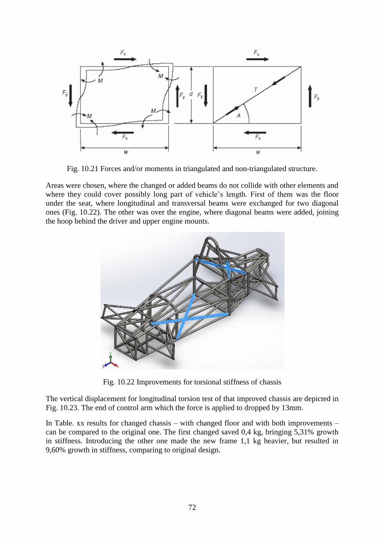
72
Fig. 10.21 Forces and/or moments in triangulated and non-triangulated structure.
Areas were chosen, where the changed or added beams do not collide with other elements and
where they could cover possibly long part of vehicle’s length. First of them was the floor
under the seat, where longitudinal and transversal beams were exchanged for two diagonal
ones (Fig. 10.22). The other was over the engine, where diagonal beams were added, joining
the hoop behind the driver and upper engine mounts.
Fig. 10.22 Improvements for torsional stiffness of chassis
The vertical displacement for longitudinal torsion test of that improved chassis are depicted in
Fig. 10.23. The end of control arm which the force is applied to dropped by 13mm.
In Table. xx results for changed chassis – with changed floor and with both improvements –
can be compared to the original one. The first changed saved 0,4 kg, bringing 5,31% growth
in stiffness. Introducing the other one made the new frame 1,1 kg heavier, but resulted in
9,60% growth in stiffness, comparing to original design.

73
Fig. 10.23 Vertical displacements for chassis with improvements
Table. 10.7
force [N] L [mm] moment
[Nm] dy [mm] angle [°] K [Nm/°]
stiffness
growth
Mass change
[kg] Mass [kg]
Stiffness per kg
[Nm/°/kg]
1000 1266 1266
14,27 0,646 1960,29 - - 49,5 39,60
13,55 0,613 2064,46 5,31% -0,4 49,1 42,05
13,00 0,589 2148,49 9,60% 1,1 50,6 42,46

74
11. EXPERIMENTAL TESTS
11.1 TORSIONAL STIFFNESS TEST
The practical test run in laboratory was based on fixing three points in the corners of the
vehicle and applying load to the fourth one in order to cause torsion of the chassis. Knowing
the load and location of fixtures and measuring deflection in four corners of the chassis it was
possible to calculate the torsional stiffness.
The test was run for frame and for full chassis assembly.
Note that during the tests the vehicle was undergoing adjustments. Engine was not fully
mounted (Fig. 11.1) what has to be taken into consideration when the results are assessed and
when laboratory and virtual tests are compared. For that reason extra virtual tests, that present
better the influence of not fully mounted engine were performed too. This way it will be
possible to compare virtual and laboratory tests and predict to some extent what would be the
results of laboratory test with the engine fully mounted. The changes made to the model in
order to run these extra tests can be seen in Fig. 11.2.
Fig. 11.1 Engine mounts that were either not welded or not bolted
Fig. 11.2 Rear part of the model representing engine not fully mounted

75
The supports were realized with three jacks. The corner located opposite to the one where
loads were applied, was additionally fixed with a chain preventing it from being lifted (Fig.
11.3). Because the jacks were equipped with rubber pads, located directly where the vehicle
was supported, deflections in all these points were expected. For that reason dial gauges
measuring dislocations in vertical direction were placed in all four corner of the vehicle.
Because of the possibility of engine not being properly fixed even on its middle mounts due to
deformations after welding required by recent adjustments, the supports were placed in front
of it. In case of full chassis assembly the jacks were placed under the uprights. In order to load
the structure plates of around 10kg each were gradually hung in the free corner. The exact
mass of the plates was taken into consideration when calculating torque acting on the
structure.
Fig. 11.3 Rear and front of the car prepared for frame laboratory tests
After collecting all the data, the calculations were conducted according to following
equations.
Eq. 11.1
Eq. 11.2
Eq. 11.3
Eq. 11.4
Eq. 11.5
where: K – frame/chassis torsional stiffness
ϕ – frame/chassis twist angle
T – torque acting on the frame
m – mass of the weight plates
g – gravitational acceleration
LF – distance between support (jack) in the front and point of load application
LR – distance between supports (jacks) in the rear
ϕF, ϕR – front and rear axis inclination
dy – vertical translation in front/rear left/right corner

76
The symbols can be compared with schemes from Fig. 11.4 (frame) and Fig. 11.5 (chassis).
Each of them depicts front (on the left side of figure) and rear part of the car supported on
rubber pads of jacks (checked rectangles) with weights placed in the front left corner.
Attention should be paid to directions of displacements dy, which explain plus and minus
signs in Eq. 11.4 and Eq. 11.5.
Fig. 11.4 Scheme of supports loads and displacements in laboratory frame test
Fig. 11.5 Scheme of supports loads and displacements in laboratory chassis test

77
11.2 STRESS TEST
Simultaneously with the torsion test stress values in the structure were supposed to be
checked to be later compared with the virtual tests’ results. For that purpose strain gauges
were placed in two points previously chosen on the basis of SolidWorks simulations (Fig.
11.6).
Fig. 11.6 Strain gauge and digital indicator used in the tests
The stresses were indicated by the software in the mode of Axial plus Bending. That means
the values stood for sum of tension along beams’ axis caused by axial forces and tension in
the walls of pipes related to bending. In order to measure the same kind of stress in the
laboratory experiment, only one strain gauge was installed on each of the pipes chosen for
test, along their axis and connected into a circuit of a quarter bridge.
Fig. 11.7 Combined tension of axial forces and bending in a beam [12]
The strain gauges had resistance of 350 Ω ± 0,30% and gauge factor of 2,04 ± 1%. The
correct connection with quarter bridge connection scheme from the indicator is presented in
Fig. 11.8.

78
Fig. 11.8 Quarter bridge scheme from digital indicator and strain gauges connection
The stress values could be calculated later as follows.
Eq. 11.6
where: σ – stress
E=210 GPa – elasticity modulus for steel
ε – strain indicated
As the indicator was displaying microstrain, με, the readings had to be multiplied by 10-6
in
order to obtain strain, ε. Stress, σ in MPa is therefore:
Eq. 11.7

79
11.3 EXPERIMENTAL FRAME TESTS RESULTS
Table 11.1 gathers average results of frame laboratory test for both torsion angle and stress
values in two points. They are represented in graphic form in Fig. 11.9 to Fig. 11.10. As the
relations they represent are linear, the trend lines intersecting the origin of coordinate system
were plotted for every graph.
Table 11.1 Results of frame laboratory test
No. of
plates mass [kg] torque [Nm]
Displacement [mm] Angle [°] Microstrain Stress [MPa]
Rear Front
Left Right Left Right Rear Front Total Ch 1 Ch 2 Ch 1 Ch 2
0 0,00 0,00 0,000 0,000 0,000 0,000 0,000 0,000 0,000 0,0 0,0 0,00 0,00
1 9,90 35,06 0,058 0,013 0,340 0,180 0,009 0,025 0,016 7,6 7,8 1,60 1,64
2 19,74 69,91 0,144 0,028 0,783 0,452 0,023 0,052 0,029 15,4 15,2 3,23 3,19
3 29,44 104,26 0,238 0,038 1,290 0,778 0,037 0,081 0,044 22,8 23,0 4,79 4,83
4 39,16 138,68 0,348 0,048 1,811 1,112 0,053 0,110 0,057 30,2 30,4 6,34 6,38
5 48,92 173,25 0,448 0,064 2,287 1,392 0,068 0,141 0,073 38,4 37,6 8,06 7,90
6 58,74 208,02 0,558 0,081 2,765 1,670 0,085 0,172 0,087 45,6 45,2 9,58 9,49
7 68,84 243,79 0,680 0,101 3,290 1,980 0,104 0,206 0,102 53,6 53,0 11,26 11,13
8 78,60 278,35 0,808 0,122 3,738 2,232 0,124 0,237 0,113 61,0 60,4 12,81 12,68
7 68,84 243,79 0,790 0,105 3,529 2,174 0,119 0,213 0,094 53,6 53,2 11,26 11,17
6 58,74 208,02 0,740 0,086 3,249 2,048 0,110 0,189 0,079 45,4 45,2 9,53 9,49
5 48,92 173,25 0,694 0,067 2,914 1,876 0,101 0,163 0,062 38,0 37,6 7,98 7,90
4 39,16 138,68 0,576 0,051 2,537 1,666 0,083 0,137 0,054 30,8 30,4 6,47 6,38
3 29,44 104,26 0,486 0,039 2,076 1,386 0,070 0,109 0,039 22,8 22,6 4,79 4,75
2 19,74 69,91 0,384 0,028 1,547 1,038 0,055 0,080 0,025 15,6 15,4 3,28 3,23
1 9,90 35,06 0,256 0,018 0,938 0,632 0,036 0,048 0,012 7,8 8,0 1,64 1,68
0 0,00 0,00 0,120 0,007 0,289 0,204 0,017 0,013 -0,003 0,0 0,0 0,00 0,00

80
Fig. 11.9 Angle and torque relation in laboratory frame test
Fig. 11.10 Torsional stiffness determined from torque-angle relation
Longitudinal torsional stiffness determined this way is 2490,5 Nm/° and constitutes 113,6%
of the value of 2191,9Nm/° determined in virtual test (boundary conditions as in experimental
test).
At that point it is worth referring again to the considerations about boundary conditions and
influence of the engine. The laboratory test was run with the engine only partially mounted
and only for one certain set of fixtures and load application. The result of 2490,5Nm/° should
y = 0,0004x
-0,020
0,000
0,020
0,040
0,060
0,080
0,100
0,120
0,00 50,00 100,00 150,00 200,00 250,00 300,00
angl
e [°]
Torque [Nm]
y = 2490,5x
-50,00
0,00
50,00
100,00
150,00
200,00
250,00
300,00
-0,020 0,000 0,020 0,040 0,060 0,080 0,100 0,120
Torq
ue
[N
m]
Angle [°]

81
therefore not be treated as exact one. This value will increase when the engine is properly
mounted. In virtual test the torsional stiffness grew by 3,8%.
Even bigger differences could be observed if the frame was supported on jacks behind the rear
suspension bay as it is normally done in such tests, as in virtual tests it caused drop by 24,3%.
Nevertheless the laboratory test shows that the real values of torsional stiffness should be
expected to be higher than the ones determined in virtual tests.
Fig. 11.11 Stress-torque relations in two chosen points of frame
The relations between stress in indicated previously points and the torque from Fig. 11.11 are
respectively 0,0461 MPa/Nm and 0,0457 MPa/Nm. For 364 Nm applied in virtual test it gives
16,8 MPa and 16,6 MPa. The real values are then 85,2% and 97,9% of the ones predicted with
the software, which proves the tests were plausible and the maximum value of 33 MPa in the
frame found with software should not be exceeded.
11.4 EXPERIMENTAL CHASSIS TESTS RESULTS
The results of laboratory torsional stiffness test, presented in Table 10.7 and Fig. 11.12 and
Fig. 11.13 gave the result of 1437,3 Nm/°, which is 22% less than in virtual tests (partially
mounted engine). Taking into consideration that the test for frame gave opposite results – the
result gained with the experimental approach was higher - and that the discrepancy is so high,
the source of that result may be the engine mounted badly after the chassis went through
adjustments. Four bolt connections were deformed after welding and the bolts could not be
fastened properly. It might have not ensured rigid connection between two parts of frame. In
frame test this connection was already behind the supports and did not influence the results.
If that value is used in Eq. 8.13 it results with just 74,12% of the rigid case’s stiffness. A bit
higher value can be expected when the engine is mounted.
y = 0,0461x
0
2
4
6
8
10
12
14
0 100 200 300
Stre
ss [
MP
a]
Torque [Nm]
y = 0,0457x
0
2
4
6
8
10
12
14
0 100 200 300 St
ress
[M
Pa]
Torque [Nm]

82
Table 11.2 Results of frame laboratory test
No. of
plates mass [kg] torque [Nm]
Displacement [mm] Angle [°] Microstrain Stress
Rear Front
Left Right Left Right Rear Front Total Ch 1 Ch 2 Ch 1 Ch 2
0 0,00 0,00 0,000 0,000 0,000 0,000 0,000 0,000 0,000 0,0 0,0 0,00 0,00
1 9,90 133,05 0,106 0,036 2,251 0,034 0,006 0,093 0,087 33,4 31,6 7,01 6,64
2 19,74 265,30 0,205 0,100 4,754 0,108 0,013 0,194 0,181 67,4 63,2 14,15 13,27
3 29,44 395,66 0,315 0,164 7,180 0,198 0,021 0,292 0,271 98,6 93,8 20,71 19,70
4 39,16 526,30 0,425 0,246 9,628 0,280 0,029 0,391 0,362 132,2 125,0 27,76 26,25
3 29,44 395,66 0,367 0,210 7,576 0,286 0,025 0,305 0,280 99,2 93,8 20,83 19,70
2 19,74 265,30 0,277 0,162 5,349 0,242 0,019 0,214 0,195 66,6 63,0 13,99 13,23
1 9,90 133,05 0,160 0,102 2,716 0,166 0,011 0,107 0,095 33,4 31,8 7,01 6,68
0 0,00 0,00 0,036 0,012 0,127 0,048 0,002 0,003 0,001 0,6 0,2 0,13 0,04
Fig. 11.12 Angle and torque relation in laboratory frame test
y = 0,0007x
0,000
0,050
0,100
0,150
0,200
0,250
0,300
0,350
0,400
0,00 100,00 200,00 300,00 400,00 500,00 600,00
An
gle
[°]
Torque [Nm]

83
Fig. 11.13 Torsional stiffness determined from torque-angle relation
The readings from strain gauges (Fig. 11.14) gave relations of 0,0527 MPa/Nm and
0,0499 MPa/Nm, which for 1266 Nm used for virtual tests results in 66,7 MPa and 63,2 MPa
and is 90,7% and 99,3% of results from virtual tests respectively. It can be assumed that this
validates the virtual test and the maximum stress value of 103 MPa obtained in it.
Fig. 11.14 Stress-torque relations in two chosen points of frame for chassis test
y = 1437,3x
0,00
100,00
200,00
300,00
400,00
500,00
600,00
0,000 0,050 0,100 0,150 0,200 0,250 0,300 0,350 0,400
Torq
ue
[N
m]
Angle [°]
y = 0,0527x
0,00
5,00
10,00
15,00
20,00
25,00
30,00
0,00 200,00 400,00 600,00
Stre
ss [
MP
a]
Torque [Nm]
y = 0,0499x
0,00
5,00
10,00
15,00
20,00
25,00
30,00
0,00 200,00 400,00 600,00
Stre
ss [
MP
a]
Torque [Nm]

84

85
12. CONCLUSIONS
The work presented analysis of chassis of a Formula Student racing car. It included virtual
analysis of suspension geometry and longitudinal torsion tests run with the finite elements
method for frame and full chassis assembly. The results of longitudinal torsion test were
verified with experimental test too. The results gathered were compared with goals set on the
basis of literature research and changes, that can be taken into consideration when a new car is
designed were suggested.
The suspension geometry test revealed that several modifications should be introduced to the
design. First of all front view control arms configuration should be modified the way, that roll
centers are lowered and stay within values suggested. Changes proposed to front view
geometry will also increase camber gain beneficially and help obtain desired camber curve in
body roll.
Attention should be paid also to wheel packaging. Incompatible hub and rim mounting holes
resulted in longer scrub radius than primarily desired. Another selection of these parts can
help keep the scrub radius and kingpin inclination within values suggested.
The structural analysis showed that the suspension supports on frame do not provide enough
rigidity. They are not located in frame’s nodes, what causes bending under forces transferred
through control arms, and can disturb suspension’s work. The design process of a frame
should start only when the suspension geometry is already designed. The designer can then
focus on providing enough rigidity to suspension bays.
The torsional stiffness determined in virtual tests proved that the chassis is not stiff enough
and with 1960,29 Nm/° reaches barely 79,62% of the theoretical case of perfectly rigid
chassis (while the goal was 90%, reached with 4524,75 Nm/°). It was however noticed that
the value determined is only a bit lower than average value of other frames, whose data was
collected for benchmarking. The reason of the low percentage is the fact that springs installed
in the vehicle are very stiff. It is recommended to revise selection of them. Structural
improvements, that increased stiffness by 9,60% to 2148,49 Nm/°.
The frame, with 49,5 kg is very heavy too. Benchmarking showed that the same or even
higher stiffness can be reached with steel frames of less than 30 kg.
The result of chassis torsional stiffness determined in experimental test turned out to be lower
than the one obtained with software. Even though in frame test the result was opposite and
real frame was more rigid than virtual. The results of chassis test might have been disturbed
by engine mounted badly after the chassis went through adjustments. It is advised to run full
chassis longitudinal torsion test again, when the frame is complete.
Analysis of twist angle along longitudinal axis of the car in frame test showed, that the rear
suspension bay is the least rigid compartment of the frame. Despite the fact, that in full
chassis test the twist angle was low there, it is important to take care of better triangulation of
this area, because it directly affects control arms and work of suspension.
The tests compared also different concepts of fixing the frame for torsion tests. It turned out
that none of the concepts ensured the same behavior of the frame as in full chassis test, which
is considered to better represent the real conditions. It is also important to run the tests,
treating engine as structural element, as it can positively influence the torsional stiffness.

86
Measurements of stress values in frame during laboratory tests verified the results of software
tests, reaching between 85,2% and 99,3% of their values.

87
13. REFERENCES
[1] Trzesniowski, Michael. Rennwagentechnik: Grundlagen, Konstruktion, Komponenten,
Systeme. Wiesbaden, Vieweg+Teubner Verlag, 2012. ISBN 978-3-8348-2209-3
(eBook)
[2] Heiβing, Bernd; Ersoy, Metin. Chassis Handbook: Fundamentals, Driving Dynamics,
Components, Mechatronics, Perspectives. Wiesbaden, Vieweg+Teubner Verlag, 2012.
ISBN 978-3-8348-0994-0
[3] Milliken, William F.; Milliken, Douglas L. Race Car Vehicle Dynamics. Warrendale,
PA, Society of Automotive Engineers, Inc., 1995. ISBN 1-56091-526-9
[4] Gillespie, Thomas D. Fundamentals of Vehicle Dynamics. Warrendale, PA, Society of
Automotive Engineers, Inc., 1992, ISBN 1560911999 (ISBN13 9781560911999)
[5] Gaffney III, Edmund F.; Salinas, Anthony R. Introduction to Formula SAE® Suspension
and Frame Design. University of Missouri – Rolla, 1997
[6] Theander, Adam. Design of a Suspension for a Formula Student Race Car. Stockholm,
Royal Institute of Technology, 2004
[7] Riley, William B., George, Albert R. Design, Analysis and Testing of a Formula SAE
Car Chassis, Warrendale, PA, Society of Automotive Engineers, Inc., 2002
ISSN 0148-7191
[8] Pang Shu-yi;Guan Xin;Zhan Jun, Research of chassis torsional stiffness on vehicle
handling performance, State Key Laboratory of Automobile Dynamic Simulation, Jilin
University, Changchun, China, 2010
[9] Thompson, Lonny L., Raju, Srikanth, Law, E. Harry, Design of a Winston Cup Chassis
for Torsional Stiffness, Warrendale, PA, Society of Automotive Engineers, Inc., 1998
[10] Abrams, Ryan, Formula SAE Race Car Analysis: Simulation and Testing of the Engine
as a Structural Member, The University of Western Ontario, Canada, 2008,
F2008-SC-005
[11] Dassault Systèmes SolidWorks Corporation, SolidWorks Education SAE Frame
Analysis, http://www.youtube.com/user/solidworks (accessed 05.03.2014)
[12] Popov, Egor P., Introduction to Mechanics of Solids, Prentice-Hall, 1968,
ISBN 0134877693