warwick.ac.uk/lib-publications

Original citation: Bove, Vincenzo and Gavrilova, Evelina. (2017) Police officer on the frontline or a soldier? The effect of police militarization on crime. American Economic Journal: Economic Policy, 9 (3). pp. 1-18. Permanent WRAP URL: http://wrap.warwick.ac.uk/90839 Copyright and reuse: The Warwick Research Archive Portal (WRAP) makes this work by researchers of the University of Warwick available open access under the following conditions. Copyright © and all moral rights to the version of the paper presented here belong to the individual author(s) and/or other copyright owners. To the extent reasonable and practicable the material made available in WRAP has been checked for eligibility before being made available. Copies of full items can be used for personal research or study, educational, or not-for-profit purposes without prior permission or charge. Provided that the authors, title and full bibliographic details are credited, a hyperlink and/or URL is given for the original metadata page and the content is not changed in any way. Publisher’s statement: Permission to make digital or hard copies of part or all of American Economic Association publications for personal or classroom use is granted without fee provided that copies are not distributed for profit or direct commercial advantage and that copies show this notice on the first page or initial screen of a display along with the full citation, including the name of the author. Copyrights for components of this work owned by others than AEA must be honored. Abstracting with credit is permitted. The author has the right to republish, post on servers, redistribute to lists and use any component of this work in other works. For others to do so requires prior specific permission and/or a fee. Permissions may be requested from the American Economic Association Administrative Office by going to the Contact Us form and choosing "Copyright/Permissions Request" from the menu. Copyright © 2017 AEA A note on versions: The version presented here may differ from the published version or, version of record, if you wish to cite this item you are advised to consult the publisher’s version. Please see the ‘permanent WRAP URL’ above for details on accessing the published version and note that access may require a subscription. For more information, please contact the WRAP Team at: wrap@warwick.ac.uk

Department Address Address Address Coventry CV4 8UW UK T (0)24 7615 xxxxx F (0)24 7615 xxxxx E youremail@warwick.ac.uk www.warwick.ac.uk 2|2

Police Officer on the Frontline or aSoldier? The Effect of Police

Militarization on Crime∗

Vincenzo Bove†

University of WarwickEvelina Gavrilova‡

Norwegian School of Economics

Abstract

Sparked by high-profile confrontations between police and citi-

zens in Ferguson, Missouri, and elsewhere, many commentators have

criticized the excessive militarization of law enforcement. We inves-

tigate whether surplus military-grade equipment acquired by local

police departments from the Pentagon has an effect on crime rates.

We use temporal variations in US military expenditure and between-

counties variations in the odds of receiving a positive amount of

military aid to identify the causal effect of militarized policing on

crime. We find that (i) military aid reduces street-level crime; (ii)

the program is cost-effective; and (iii) there is evidence in favor of a

deterrence mechanism.

JEL classification: K42, H49, H76

Keywords: police, crime, militarization

∗The authors wish to thank Stella Chatzitheochari, Claudio Deiana, Mirko Draca,Matthew C. Harris, Giovanni Mastrobuoni, Roberto Nistico, and Floris Zoutman, forhelpful feedback. We are also grateful to the journal’s editor, John Friedman, and threeanonymous reviewers for constructive suggestions that helped us improve the article.The usual disclaimer applies.†v.bove@warwick.ac.uk‡evelina.gavrilova@nhh.no

1

I Introduction

In recent years, the Law Enforcement Support Program (LESO) in the US

has been the subject of considerable political controversy. This program,

known as the “1033 Program”, is a federal initiative that, since 1997, has

transferred more than $4.3 billion worth of surplus military equipment from

the Department of Defense to domestic police agencies across the US. The

program came under scrutiny in the summer of 2014, following the fatal

shooting of an unarmed 18-year-old African-American by a police officer;

and an ensuing series of protests in the city of Ferguson, Missouri. In

the aftermath of the protests, Ferguson’s police force used military-grade

weapons and armored tactical vehicles - believed to be acquired through

the “1033 Program” - to quell the riots. The perceived disproportionality

of the reaction of law enforcement has sparked a contentious debate about

the consequences of giving military capabilities to local police forces.

We investigate the causal effect of an increase in the militarization of

US local police forces on their effectiveness in preventing and solving crime

and, with Harris et al. (2016), we provide the first empirical analysis of the

consequences of the 1033 Program. To what extent has the proliferation

of military weapons within US local police forces affected their effective-

ness in countering crime? Has the acquisition of military-style equipment

contributed “to the protection of the public” and provided “effective and ef-

ficient contributions to public safety” (White House, 2014, p.6)? Although

these questions have crucial policy implications for security policies, they

have so far remained unanswered.

We use newly released data by the US Department of Defence on more

than 176,000 transfers of equipment held by 8,000 local police agencies over

the period 2006-2012. We explore whether this military grade equipment

has a tangible effect on the production function for law enforcement, mea-

sured by crime and arrest rates. These two variables allow us to disentangle

the deterrence effect produced by the display of military equipment from

the efficiency effect when the police use military equipment to solve more

crime and arrest perpetrators. Our data allow us to explore the black box

of policing by observing whether inputs to the physical stock of capital have

an effect on the quantity and efficiency of police personnel. Additionally,

2

we investigate whether there is a discernibly different effect between lethal

vs. non-lethal equipment transfers by exploring variation in the type of

military hardware redistributed.

To identify the causal effect of militarized policing on crime, we interact

exogenous time variation induced by military spending and local variation

between counties in the likelihood of being an aid recipient. High military

spending, driven by international factors such as the war in Afghanistan,

caused the Department of Defence to accumulate excess reserves during

high spending years. The “1033 Program” allows the reallocation of this

excess property to law enforcement agencies across the country. We in-

teract this variable, which varies over time, with a county’s time-invariant

propensity to acquire military aid, measured as the fraction of years that a

county receives a positive quantity of equipment. Our identification rests

on a comparison between frequent and infrequent recipients, in years fol-

lowing high military spending to years following low spending, similar to a

difference-in-difference approach.

We find that military aid reduces crime rates. In particular, more mil-

itary aid leads to a decline in robberies, assaults, larcenies and motor ve-

hicles thefts, which are all part of the so-called “susceptible crimes” (a

la Draca et al. , 2011), i.e., crimes that are more likely to be prevented

by police visibility. By the most conservative estimate, a ten percent in-

crease in aid reduces total crime by 5.9 crimes per 100,000 population.1

Although the magnitude of this effect is relatively small, 0.24% of the aver-

age crime rates in treated areas (2470 crimes), the annual average value of

aid acquired by a county is around $58,000, suggesting that this is a very

inexpensive crime-reducing tool. Our results survive a variety of robustness

checks such as population weighting, differential county crime trends, and

alternative instruments such as US military fatalities.

When we focus on police activities, we find essentially no effect of aid

on arrest rates. We further find that the observed effects on crime are

not explained by an observable increase in police manpower. Yet, we do

find that an increase in the military aid might lead to release of employees

of law-enforcement agencies, suggesting that labor and capital could be

1Note that throughout the article we always refer to units of crime per 100,000population, even when this is not explicitly stated.

3

considered substitutes for some of the activities of the police. Furthermore,

we do not find evidence of an effect of military aid on injuries and assaults

on police officers. Crucially for the causa of recent public debate, we find

no effect on the number of offenders killed.

Taken together, our results suggest that employing military equipment

improves the capabilities of law enforcement to deter crime, potentially

through an unobservable police effort channel. Our cost-benefit analysis

shows that, for a ten percent spending increase, around $5,800 per county

per year, the crimes deterred amount to a social benefit of roughly $112,000.

Our results partially mirror those of Harris et al. (2016), who similarly find

that receiving tactical items leads to a reduction in property crime rates.

Interestingly, this study also finds that military aid brings a reduction of

the assaults on police officers, the number of complaints against them, and

an increase of arrest rates for drug and weapons charges.

Our study is closely related to the empirical literature on the causal

effect on crime of an increase in the funds provided to the police force (see

Chalfin & McCrary, 2014, for a recent review). Machin & Marie (2011)

find a decrease in robbery rates following the increase in targeted funds

to police forces in England and Wales. Evans & Owens (2007) find a

decline in auto theft, burglary, robbery, and aggravated assault following

receipt of grants to hire police officers. Similarly, in order to identify the

effect of an increase in the labor component of the production function of

the police, several studies have exploited temporary redeployment policies

arising from terror-related events (Di Tella & Schargrodsky, 2004; Klick &

Tabarrok, 2005; Draca et al. , 2011). Yet, none of these studies tackles the

effect of an increase in police equipment on crime.2 Our study therefore

contributes to the literature more broadly by specifically focusing on the

effect on crime rates of more “capital”, rather than more “labor”.

This paper is structured as follows: Section II provides some insights

into the 1033 Program; Section III presents our data and Section IV ex-

plains our identification strategy. Section V describes our results and Sec-

tion VI offers concluding remarks.

2The only exception is Mastrobuoni (2014), who investigates whether differences inclearance rates across two police forces in Milan can be attributed to the availability ofadvanced Information Technology strategies. He finds that this is indeed the case, andthat adopting IT innovation doubles the productivity of policing.

4

II The “1033 Program”

In 1990, following several years of increasing crime levels, the US Congress,

through the National Defense Authorization Act, authorized the transfer of

excess property from the Department of Defense to federal and state agen-

cies, mainly for counter-drug related activities. The Congress made the

program permanent in 1997, expanding its scope by allowing law enforce-

ment agencies to acquire military property to assist in arrest and apprehen-

sion tasks, whilst retaining a focus on counter-drug and counter-terrorism

requests. The program was renamed the “1033 Program” in 1996, following

the replacement of Section 1208 with Section 1033. The program is under

the jurisdiction of the Defense Logistics Agency (DLA) and is overseen by

the Law Enforcement Support Office (LESO), located at DLA Disposition

Services Headquarter.

Law enforcement agencies follow a three-step procedure to acquire mil-

itary hardware: (1) they obtain the approval of the State Coordinator and

LESO to participate in the program; (2) they place requests and provide

justification for specific items. Requests are screened by the State Coor-

dinator and the LESO Staff; (3), law enforcement agencies then receive a

decision and if their request is approved, they must cover all transporta-

tion and/or shipping costs in connection with the receipt of the equipment.3

Since the inception of the “1033 Program”, over 8,000 federal and state law

enforcement agencies have requested a variety of equipment, from assault

rifles and grenades to Mine Resistant Ambush Protected (MRAP) vehicles,

helicopters and drones, to non-lethal equipment, such as high-tech cameras,

camouflage/deception equipment and office supplies.

It was not until media coverage of the Ferguson unrests, however, that

the program drew media and public attention. Since the Ferguson incident,

there has been much debate on whether local authorities’ response to crime

is often disproportionate and why e.g., the police force in a city of 20,000

residents looked like an invading army engaged in urban warfare against

street protesters.4

3We refer the readers to Harris et al. (2016) for a more detailed discussion ofthe allocation process. See also http://www.dla.mil/DispositionServices/Offers/

Reutilization/LawEnforcement/ProgramFAQs.aspx4See Amanda Taub, Why America’s police forces look like invading

5

In 2014 US President Barack Obama ordered a review of the distribu-

tion of military hardware to police agencies (Reuters, 23/08/14). Following

this request, the White House released a report stating that while military

equipment has “contributed to the protection of the public and to reduced

operational risk to peace officers [..] when police lack adequate training,

make poor operational choices, or improperly use equipment, these pro-

grams can facilitate excessive uses of force and serve as a highly visible

barrier between police and the communities they secure” (White House,

2014, p. 6). Consequently, by an executive order federal transfers of cer-

tain types of military-style gear to local police departments were banned

in 2015.5

III Data

To address the question of the effect of military equipment on the activity

of the police force we use Uniform Crime Reports (UCR) data at the county

level and Law Enforcement Officers Killed and Assaulted (LEOKA) data at

the agency level. Crime in the United States is reported by law-enforcement

agencies to the FBI, which creates summaries of these reports published as

annual statistics. The Interuniversity Consortium for Political and Social

Research (ICPRS) aggregates the separate agencies into counties, taking

into account issues such as agencies spanning several counties, agencies not

reporting for certain periods and agency closures and openings.

The UCR data allows us to distinguish between several major crime

categories such as homicide, assault, robbery, burglaries, larceny and motor

vehicle theft. The LEOKA data allows us to look for an impact of military

aid on law-enforcement characteristics such as the numbers of officers and

civilian employees at the agency, the ratio between them, the number of

calls received by the police, injuries, assaults suffered by the police and

the number of offenders killed. Recently, Chalfin & McCrary (2013) raised

armies, Vox, Aug. 19, 2014, http://www.vox.com/2014/8/14/6003239/

police-militarization-in-ferguson5President Barack Obama ordered a ban on grenade launchers, tracked armored

vehicles, armed aircraft, guns and ammunition of .50 caliber or higher, and restrictionsto the transfer of wheeled armored vehicles, drones, helicopters, firearms and riot gear,to ensure that officers are trained in their use (Washington Post, 18/05/2015).

6

concerns about the measurement error in UCR police records. We have no

reason to assume that this measurement error is associated with the amount

of military aid received. In addition, note that we drop eight percent of

the crime data due to missing control variables for some counties.

Data for the amount of military aid awarded to each county have been

recently released by the US Department of Defense and are now available

in the public domain.6 We use the DLA’s federal supply category and class

name to identify the type of equipment. We then aggregate several cate-

gories into four groups: weapons (e.g., explosives, guided missiles, guns),

vehicles (e.g., aircrafts, combat, assault, and tactical vehicles, including

their components), gears (e.g., communication devices, special clothing,

night vision equipment) and a residual category (e.g., office supplies, fur-

niture, plumbing items). Table A.1 shows our classification categories, and

the relative frequency of each category as well as the average value of each

acquisition. We use information about the original acquisition value that

was paid by the military services for the equipment.7

We also use information on the poverty rate, median income, unemploy-

ment rate, the size of the population, and the shares of males, blacks, and

people between 15-19, 20-24, 25-29 and 30-34 years old. These covariates

capture both individual criminal decision-making analysis and heteroge-

neous trends across counties. The data are taken from the US Census

Bureau and the US Department of Labor. Table 1 offers summary statis-

tics for the main variables of interest as well as for the control variables.

The table shows that, although each county in our sample experiences ap-

proximately 2500 crimes per 100,000 population every year, most of these

crimes are burglaries and larcenies, whereas homicide is a much rarer event.

All military aid is recorded as quantities and acquisition value per unit; ac-

cording to our data, a county on average receives equipment worth $58,000

per year. As one would expect, the most expensive items obtained through

6In Figure A.1 we show the monetary value of the given aid for the years in thesample period. In the period between 2006 and 2012, the value of military donations tolaw enforcement agencies went from slightly less than $30 million to almost $500 millionper year, thus expanding significantly. It then reached $750 million in 2014.

7We prefer not to use quantities (e.g., 10 guns over 30 mm up to 75 mm), as in eachcategory, different classes of aid have very different values (e.g., helicopters vs tractors).The same applies to the other categories, but as a robustness check, we do replace valueswith quantities.

7

the 1033 Program are vehicles, such as aircraft, watercraft and armored

vehicles, and the most commonly requested items are gear, for example

clothing.

—————— [Table 1 in here] ——————

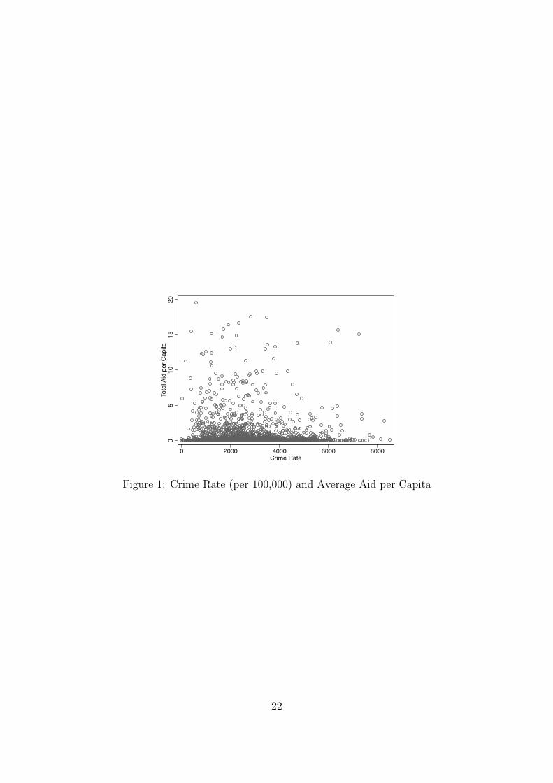
Figure 1 presents the scatter plot of military aid per capita and crime

rate. Although counties with higher crime rates should be more likely to

request support by the federal government, there is almost no association

in the aggregate between the crime rate and the total value of military aid

per capita acquired by counties. We therefore now turn to the presentation

of the empirical strategy that will allow us to find the effect of equipment

on crime.

—————— [Figure 1 in here] ——————

IV Empirical strategy

We are interested in the coefficient β from the following model:

Yc,t = βEquipmentc,t−1 + γ‘Xc,t + αc + ηs,t + εc,t (1)

The outcome variable Yc,t is the crime rate for county c in year t whereas

Equipmentc,t−1 is the monetary size of the military equipment that has

been acquired by the county. We use a linear-log model i.e., we take the log

values of Equipmentc,t−1 and we keep Yc,t in its original scale.8 We lag the

values of aid by one year to allow time for the equipment to be transferred

and placed into use.9 Xc,t is a vector of control variables described in section

III. County fixed effects αc absorb county-specific constant features such as

geographical location. It is reasonable to assume that particular counties,

such as those belonging to border states, could display a positive correlation

8Note that 21 percent of the counties did not receive any aid in the period underconsideration. We therefore use the transformation log (1 + Equipment). It is easy tocheck that log (1 + Equipment) ≈ log (Equipment) for numbers around the minimumvalue of most equipment. This specification is useful in the presence of diminishingmarginal returns and it is easy to interpret.

9We do not use more than one lag as the federal government requires agencies thatreceive 1033 equipment to use it “within one year of receipt” (White House, 2014, p.7).

8

between crime rate and the amount of aid received because of state-specific

effects. For example, states at the Mexican border require more resources

to control drug-smuggling, have higher crime rates than other states, and

are therefore more likely to request aid from the DoD. This state-specific

effect would give a positive bias to β, yet changing political policies make

this effect time-variant. We thus interact state fixed effects with time fixed

effects ηs,t, which allows us to control for state-specific policies and the

common factor in aid delivered to counties within a given state at a given

point in time.

Theoretically, an effect of aid on crime could be channeled through po-

lice manpower and through responses of criminals. A significant effect of

equipment on police and crime would constitute evidence for the former.

To verify whether an effect of aid on the crime rate might be driven by

increased police efficiency, we attempt to capture clearance rates by using

arrest rates as dependent variable and comparing the resulting coefficients

with those on crime rates. We also look at additional police outcomes

through the LEOKA data.10 If there is an effect of aid on police outcomes,

note that equation 1 with crime rates as dependent variables will resemble

the reduced form in a two stage model estimating the elasticity of crime

with respect to police characteristics, which would be comparable to previ-

ous literature (see Chalfin & McCrary, 2014). If the effect of aid on crime

is driven by responses of criminals, and not by observable police responses,

we would find an effect only on crime rates.

There could be an ex-ante positive correlation between the crime rates a

county experiences and the amount of military aid it requests. To alleviate

this concern, we employ an IV estimation method by using US military

spending in the previous year. By law, the “1033 Program” allows local

police forces to acquire excess property from the Department of Defense.

When US military spending is high (e.g., due to an increase in the intensity

of the war in Afghanistan), this generates an accumulation of military

hardware. This, in turn, increases the amount of military aid that can be

delivered to local law enforcement agencies.

10Note that the dependent variable from the LEOKA data is at the level of thereporting agency, whereas X and Equipment remain defined at the (geographicallylarger) county level.

9

Given that US military spending exhibits only time variation we follow

the same procedure as Nunn & Qian (2014). We create an instrument

by interacting US military spending with a county’s tendency to receive

military aid from the federal government.11

The first stage is then:

Equipmentc,t = α+θ

[USMilext−1×

(1

7

2012∑t=2006

Pct

)]+δ‘Xc,t+α

2c+η2s,t+υc,t

(2)

where USMilext−1 is US military spending in constant US$ and Pct is a

dummy for whether c received any military aid in year t. Conceptually, we

have two sources of variation. We have identification along the extensive

margin of whether aid is received and along the intensive margin of how

many items are received. The former variation is captured by the probabil-

ity of aid receipt, allowing us to compare crime responses between counties

that have received aid for the same number of years. Naturally, this gives

the IV a mechanical positive correlation to the dependent variable in the

first stage, which is, however, alleviated by the inclusion of county fixed

effects, absorbing the probability factor in the instrument. This leaves

the variation in military expenditure to aid identification through its effect

on the intensive margin. As Nunn & Qian (2014) make clear, this strat-

egy resembles a difference-in-differences estimation strategy, where in the

first-stage (and in the reduced-form) we compare counties that frequently

receive aid to counties that rarely receive aid, in years following high US

military spending relative to years following lower military spending. The

main difference from a difference-in-differences strategy is that our treat-

ment variable is continuous.

Our identification strategy is based on the premise that, conditional on

other contextual variables, our instrument has an impact on the crime rate

only through the provision of military equipment. Note that the exclusion

restriction is not violated if higher US military spending affects crime rates

through its national or regional influence on e.g., voluntary military re-

11Nunn & Qian (2014) investigate the effect of US food aid on conflict by usingexogenous variations in US wheat production and in recipients’ tendency to receive apositive amount of US food aid.

10

cruitment, as the inclusion of state-year fixed effects and control variables

flexibly account for any national or state-specific changes over time. Note

also that neither our instrument nor the crime rate in US counties displays

monotonic trends, thus ruling out the possibility of a spurious correlation.12

Figure 2 presents a comparison between counties that have received aid

only once or two times, denoted as low recipients, and counties that have

received aid at least three times throughout the sample period, denoted

as high recipients. Each group makes up about 40% of the sample. We

observe a decrease in crime for both groups of counties, yet this decrease is

more pronounced for the high recipients (Figure 2a); this is consistent with

the fact that high recipients display a more marked increase in the amount

of military aid they acquire in relation to total surges in available military

hardware (Figure 2b). Figure 3 presents a taste of our results in the first

and second stages of our IV approach. We observe a remarkable positive

correlation between total military aid and our instrument. We also observe

a substantial negative relation between the fitted values of total aid and

crime rate.

—————— [Figure 2 in here] ——————

—————— [Figure 3 in here] ——————

V Results

In this section we first examine the impact of military aid on crime and

arrest rates; we also discuss the degree to which our estimates can be

interpreted as providing evidence of deterrence; additionally, we try to

establish the extent to which distinct crimes such as robbery and assault

respond differently to increases in each category of military aid such as

12On one hand, although the US has experienced a general decline in crime rates inrecent years, there is a lot of heterogeneity across counties and some categories of crimesuch as burglaries and larcenies have hardly seen significant changes in the aggregateover time. At the same time, both military spending and the number of US militarycasualties per year display an inversely U-shaped pattern. Moreover, the interactionbetween US military spending (or casualties) and Pct gives lower weights to countieswith arguably less crime i.e., those that have requested/received aid less frequently.Thus, assuming that the relation is spurious, if the resulting coefficient is negative, itwould have an upward bias toward 0.

11

weapons and vehicles; we then present results from a variety of robustness

tests; and we conclude with a basic cost-benefit analysis.

A Does aid affect crime rates?

Our first question revolves around the existence of a causal effect of military

aid on crime. Table 2 incorporates the baseline model. Column 1 presents

the reduced form relationship between aid and crime. We find that a naive

OLS estimation would not reveal any influence of aid on crime, which

is consistent with Figure 1.13 Column 2 shows the first stage estimates.

As expected, we find that an increase in the military expenditure of the

previous year - holding aid receipt probability constant - leads to a higher

amount of aid received by the county. The Kleinbergen-Paap F-Statistic is

similar to the conventional F-statistic, but takes into account the clustering

of the standard errors, with a value of 49, above conventional levels that

characterize weak instruments.

Column 3 of Table 2 shows that military aid reduces the total number

of crimes: a ten percent increase in the total value of military aid leads to

a decrease of 5.9 crimes per 100,000 population. The negative coefficient

reveals that our prediction that the positive correlation between aid and

crime could bias the naive OLS estimates upward, as in column 1, was

correct.

Further, reading across the first row of results in Table 2, we find that

this reduction can be attributed to a decrease in robberies, assaults, bur-

glaries, larcenies and motor vehicle thefts. The effect is very pronounced

for street-level crime types, like larceny and vehicle theft, whereas it is

insignificant for homicide. This suggests that military aid could have a de-

terrent effect based on greater visibility. This “display” mechanism could

deter crime by increasing the subjective probability of arrest.

On the last line of Table 2, we present estimates of the elasticity of crime

with respect to the value of equipment. The biggest elasticity we observe

is -.15 for robbery, followed by motor vehicle theft with -.09, assault -

13We report the results for the control variables in Table A.2 in the Appendix. More-over, in Table A.3, we show the OLS estimates of the effect of military aid on allcategories of crime, which are all consistent with the absence of a statistically significanteffect.

12

.236 and -.023 for the total crime rate.14 These elasticities are well within

the boundaries of -.01 to -2 presented in previous literature (Chalfin &

McCrary, 2014). They are smaller than Evans & Owens’s (2007) elasticities

of crime with respect to the size of the police force, between - .26 and - .99,

also based on US data.

—————— [Table 2 in here] ——————

B Is the effect of aid on crime driven by police ef-

forts?

In this subsection we explore several potential channels through which aid

could influence crime reduction. We first establish the effect of aid on arrest

rates. If military aid increased police efficiency and ability to solve crimes,

then we should find that the number of arrests increases relative to the

crime rate. Moving across the columns of Table 3, we do not find strong

support for an effect of military equipment on the number of arrests. On

the one hand, the substantive effect is negligible, and, e.g., a ten percent

increase in total aid leads to a 0.16 decrease in the number of arrests for

robbery per 100, 000 population. On the other hand, the decline in the

number of arrests could be fully attributed to the decline in the underlying

crime rate.15 Therefore, it seems that military aid does not improve the

arresting performance of local police units, thus revealing that it most likely

helps to deter individuals from participating in illegal activities in the first

place.

—————— [Table 3 in here] ——————

Table 4 captures other ways in which law-enforcement can alter the ar-

rest perceptions of criminals. The dependent variables are the number of

police officers, the number of civilian employees, the ratio between officers

and civilian employees, the number of received calls, the number of injuries

14Running a log-log model yields virtually the same elasticity.15In fact, when we control for crime rate, the effect of military aid on the number of

arrests becomes insignificant at the conventional level. We do not explicitly include thisadditional model though, as crime rate is endogenous to military aid, and can constitutean improper control.

13

or assaults in the line of duty, and the number of offenders killed by the

police. As we can see, military aid might influence hiring decisions by in-

ducing law enforcement agencies to devote more resources to hiring of new

police officers and civilian employees. If labor and capital are substitutes

in the police production function, then the increase in available capital

might lead to a decrease in the labor employed. Whereas the number of

officers declines by a very small magnitude, the number of civilian em-

ployees declines by 0.2 for a ten percent increase in the size of the military

aid. Moreover, military aid neither affects police activities measured by the

number of calls they receive nor has a significant impact on the number of

police officers assaulted or injured in the line of duty; it also does not have

an effect on the number of offenders killed by the police.

To further check the existence of alternative channels linking the “1033

Program” to police performance, we look at the effect of aid on citizens’

complaints. One of the most popular arguments against the militarization

of the police forces is the probability of a disproportionate use of aggressive

weapons and tactics on undeserving targets which can undermine a pro-

ductive and trustworthy interaction between the police and the local pop-

ulation. If subscribing to this claim, we would observe a positive impact

of aid on citizens’ complaints. Yet, as Harris et al. (2016) point out, mil-

itary hardware may also reduce complaints if citizens are too intimidated

to express dissatisfaction with the behavior of the police. We therefore

consider the impact of the 1033 Program on the number of citizen com-

plaints, compiled from published annual reports of police departments, and

made available by Harris et al. (2016). The last column of Table 4 shows

that acquiring military items has a negative effect on complaints, yet not

significant.

Therefore, it seems that the deterrent effect observed in Table 2 comes

either through a response of the supply side of the market for crimes, that is,

criminals themselves refrain from crime or there is an unobservable police

effort component not captured by our indicators. Military aid therefore

seems to lead to a reduction in crime rates mainly through a deterrence

mechanism.

Taken together, our results are similar to those of Harris et al. (2016).

Both studies find a decrease in robberies, assaults and vehicle thefts, albeit

14

Harris et al. (2016) find bigger effects. Both studies also find a negative

effect of tactical equipment on citizen complaints. Finally, Harris et al.

(2016) find a negative effect on the clearance of motor vehicle theft crime;

whereas we also find a negative effect of military aid on overall arrest rates,

the magnitude of the coefficients in our models is very small. The differ-

ences between our findings and those of Harris et al. (2016) should be

considered in light of the peculiar operationalization of military aid (Harris

et al. (2016) use the quantity rather than the value), the different sample

size, the choice of the control variables and, perhaps more importantly, the

heterogeneity of treatment effects. We use two conceptually distinct instru-

ments and it is likely that in our framework the subset of “compliers” is

different from that in Harris et al. (2016). While Harris et al. (2016) filter

the effect for counties which are more sensitive to transportation costs, we

give more weight to recipients in high spending years.

—————— [Table 4 in here] ——————

C Which type of military aid is the most constructive

in combating crime?

Our third question relates to the existence of distinctive effects of different

categories of military aid on crime rates. This is a crucial question in light

of the recent heated debate on the questionable use of military weapons and

tactics by the police forces. We restrict our attention to aggregate crime

as well as to the crime indices which were found to be significantly affected

by aid (Table 2). Results are reported in the Appendix, Table A.4, which

shows a sort of hierarchy in the marginal impact of aid on crime: the resid-

ual category, labeled “others”, which includes only non-lethal equipment,

without military attributes, has the biggest marginal effect on the reduc-

tion of crime. This is most evident in the fifth panel of Table A.4, where a

ten percent increase in this category reduces the total number of crimes by

almost seven units per year. The second class of items is vehicles, and the

final one is gears, where the effects found do not seem to be significantly

different than for the effect for Total Aid.16 Two basic implications emerge:

16 In Table A.4, we also present the p-values for a Wald test for difference in thecoefficient of the row variable with the coefficient on “Lagged Total Aid”.

15

firstly, two highly visible tools, gears and vehicles, have strong and sizable

effects on all the types of crime. Although vehicles are easily detectable,

note that gears include sophisticated electronic equipment, training aid

and, in almost half of the instances, clothing. This is consistent with early

studies by e.g., Bell (1982), which explore how police wearing military-style

uniforms influences citizens’ perception of the police’s authority and legiti-

macy, and reinforces the notion that a main causal channel could be based

on perceptual deterrence. Secondly, even though the residual category is

still too aggregate and too large to make reasonable claims about which

of its subcomponents are driving the effect, the inclusion of diverse office

equipment could entail that law enforcement agencies are able to improve

the efficiency of their organizational practices and, therefore the alloca-

tion of their time resources, resulting in more patrols or other unobserved

crime-deterring activities. Additionally, the inclusion of IT hardware in

the residual category might ultimately lend support to previous findings

by Mastrobuoni (2014) on how IT adoption (or innovation) affects crime.17

Although weapons do not appear to work as a deterrence tool, note

that our instrument seems to be weak at predicting the allocation of the

weapon category. This applies to all the four sub-categories of crime in

which we are interested as well as to the overall crime level. It seems that

our instrument does not capture well the allocation decisions related to

weapons in high spending years, most likely pointing to a caution from the

policymaker associated with the controversy on the value-added of using

battlefield weapons to police urban areas.

D Robustness Checks

We verify our findings with a round of additional checks. We omit tables

due to space limitations, although all additional models can be found in

the online Appendix. Table A.5 limits the underlying sample to counties

in which the mean population size is lower than 250,000 inhabitants, and

where the unemployment rate, the poverty rate, the median income within

a county and the share of blacks are higher than the national median.

17As aid without clear military attributes is not the focus of this article, however, weleave this facet to future research.

16

Exploring various cuts, we can see that the control variables are not sub-

stantially driving our results and neither can we report a heterogeneity in

the effect of aid on crime.

In Table A.6, panel A, we replace the value of military aid by its quan-

tity. Our results remain significant, thus lending additional support to

previous results. Note that we cannot explicitly comment on the substan-

tive effects as each category contains highly heterogeneous items. Panels

B and C of Table A.6 exploit alternative, yet related, instruments, such as

the interaction between the probability of receipt and the amount of mili-

tary spending in percentage of GDP or the total number of US fatalities in

Afghanistan and Iraq (instead of the level of US military spending). The

rationale behind the inclusion of the share of output devoted to the mili-

tary, also called the military burden, is that it measures the priority given

to defense rather than to military power or the absolute level of military ex-

penditure (Smith, 2009). As we can see, the coefficients are significant and

in the same order of magnitude as in Table 2. Using US military casualties

as an alternative instrument allows us to effectively capture the intensity

of military deployments and the severity of war, which, in turn, influence

the procurement of military equipment. Again, previous findings about aid

and crime are strongly borne out by this new set of empirical results. The

coefficients are similar to our baseline models and the F-statistics are above

conventional levels.

In Table A.7, panel A, all results are weighted by the size of the mean

population to reflect crime as a population mean, and, by and large, the

results carry over. In fact, the coefficients are now distinctly higher, and

still statistically significant. In panel B we replace total aid by its per

capita counterpart, and the coefficients retain the same magnitude and

are statistically significant. In panel C we keep a subsample of counties

that contain law-enforcement that have fully complied with Uniform Crime

Reports reporting, that is, with 100 percent coverage of reported crime.

We, however, drop almost half of the observations and find that the results

on robbery, assault and vehicle-theft survive this robustness check.

In the last table (Table A.8), we account in different ways for preex-

isting trends in crime. In panel A we include year fixed effects instead of

the interaction between year and state fixed effects, whereas in panel B we

17

include county-specific linear trends to the baseline specification and we

exclude state-time dummies. In this way we account for differential crime

trends across counties. On both exercises our baseline results remain un-

affected and, if anything, accounting for differential crime trends leads to

higher effect sizes. Finally, in panel C, we only focus on counties which

have received a positive amount of aid for at least one year and for less

than seven years. The purpose of this exercise is purely mechanical as we

want to show that our effects are not driven by the most frequent recip-

ients of aid. We find the same effects, with a first stage coefficient that

is higher than the one estimated in the baseline model. Intuitively, the

variation in such counties is more likely to be absorbed by the fixed effects,

which explains why the absence of these counties has such a small impact

on the estimated coefficient in the first stage and leads to an increase of

the same coefficient. To further demonstrate this, consider Figure A.2, a

binned scatterplot for the first stage by different probabilities of receiving

aid. The Figure shows that the relationship between the instrument and

Total Aid is more positive for counties that received aid in two, three or

four years out of seven.18 Hence, exploring various estimation techniques

and specifications, we feel confident to conclude that military aid reduces

crime, and that the effect may be driven by a deterrence mechanism.

E Cost and Benefit Analysis

We perform a basic cost-benefit analysis by comparing estimates from our

baseline models (Table 2) with estimates of the social cost of particular

crimes. Heaton (2010) provides one of most recent reviews of academic

research on the cost of crime in the US, including accounting-based methods

(all the individual costs borne by individuals and society) and contingent

valuations (what individuals are willing to pay for crime reduction). He

summarizes the cost estimates from three studies of the cost of crime,

two using accounting-based methods (Cohen & Piquero, 2009; McCollister

et al. , 2010) and one using contingent valuation (Cohen et al. , 2004). He

calculates that the average cost of a robbery is $67,277 (in 2007 US dollars),

18Figure A.2 also suggests a lack of mechanical positive bias between the instrumentand the instrumented variable, otherwise the fit lines would be arranged with sevenyears as the highest positive slope and one year of aid as the lowest.

18

of a serious assault $87,238, of a burglary $13,096, of a larceny $2,139 and

of a motor-vehicle theft $9,079. By our baseline and most conservative

models (Table 2) a ten percent increase (around $5,800) in the value of

aid reduces robberies by almost 0.6 units, assaults by 0.5 units, burglaries

by 0.9 units, larceny by 2.7 units and vehicle thefts by 1.2 units. This

means that the benefit of a ten percent increase in aid is roughly $112,000,

compared to a cost of $5,800, making the donation of military equipment

a good investment.

VI Conclusions

In 1990 the US Congress enacted the National Defense Authorization Act,

later called the “1033 Program”, allowing local law enforcement agencies to

acquire excess property from the Department of Defense, including drones,

military weapons and armored vehicles. The program came under severe

scrutiny in 2014, following a wave of public protests against the dispropor-

tionate use of military tools by local police forces. By most reports, provid-

ing military equipment free of charge encourages hyper-aggressive forms of

domestic policing, which can increase tension, mistrust and uncooperative

behaviors between local police departments and local communities. Yet,

so far there have been no attempts to examine the tangible outcomes of

issuing military equipment to law enforcement agencies, not even its effect

on crime rates.

Using panel data for US counties over the 2006-2012 period, we provide

quantitative evidence on the effect of the “1033 Program” on police perfor-

mances. En route, we complement the economic literature on the determi-

nants of policing. Our identification strategy relies on exogenous variation

in timing and size of military spending to test whether the militarization

of local police forces improved their performances. The results reported

in this article provide evidence of a positive effect of military hardware on

crime rates, most likely via a deterrence mechanism. We run a number of

additional models to isolate this mechanism from other competing channels

such as various measures of observable police effort. Interestingly, although

all the non-lethal categories of aid are effective in preventing crime, this

effect is not reflected in a shift in observable police characteristics such as

19

arrest rates, manpower or others, hinting at a possible alternative effect

channel of unobservable police effort.

The empirical literature on police resources and crime and most of the

public debate on this issue, assume that additional resources are allocated

to increase the size of the police force. Therefore, implicitly police costs are

labor costs. Yet, there is an important capital component in the production

function for law enforcement that is usually neglected, regardless of whether

new equipment is bought, provided for free or acquired at a greatly reduced

price. We estimate that a ten percent increase in the value of military aid

reduces the total number of crimes by 5.9 units. Despite a small total effect,

the program is quite cost-effective, and adding an extra $5,800 in overall aid

leads to a drop of roughly $112,000 in the social costs of robberies, assaults

and vehicle thefts combined. Our results seem to suggest that the returns

per dollar spent on the margin to capital might be even higher than for

labor, and this is an issue that certainly deserves further empirical research.

That said, taken together, our results do not directly provide evidence in

favor of or against the possibility that military equipment contributes to

overly aggressive approaches by police units, which can in turn escalate to

a standoff between urban communities and the officers that police them.

This is a social cost that our analysis cannot duly capture and it is an

important point for future research.

References

Bell, Daniel J. 1982. Police uniforms, attitudes, and citizens. Journal of criminal justice,

10(1), 45–55.

Chalfin, Aaron, & McCrary, Justin. 2013. Are US Cities Under-Policed? Theory and

Evidence. NBER Working Paper, 18815.

Chalfin, Aaron, & McCrary, Justin. 2014. Criminal Deterrence: A Review of the Liter-

ature. Tech. rept. Working paper May.

Cohen, Mark A, & Piquero, Alex R. 2009. New evidence on the monetary value of saving

a high risk youth. Journal of Quantitative Criminology, 25(1), 25–49.

Cohen, Mark A, Rust, Roland T, Steen, Sara, & Tidd, Simon T. 2004. WILLINGNESS-

TO-PAY FOR CRIME CONTROL PROGRAMS. Criminology, 42(1), 89–110.

20

Di Tella, Rafael, & Schargrodsky, Ernesto. 2004. Do police reduce crime? Estimates

using the allocation of police forces after a terrorist attack. The American Economic

Review, 94(1), 115–133.

Draca, Mirko, Machin, Stephen, & Witt, Robert. 2011. Panic on the streets of london:

Police, crime, and the july 2005 terror attacks. The American Economic Review,

2157–2181.

Evans, William N, & Owens, Emily G. 2007. COPS and Crime. Journal of Public

Economics, 91(1), 181–201.

Harris, Matthew C, Park, Jin Seong, Bruce, Donald J., & Murray, Matthew N. 2016.

Peacekeeping Force. Effects of Providing Tactical Equipment to Local Law Enforce-

ment. University of Tennessee.

Heaton, Paul. 2010. Hidden in Plain Sight: What Cost-of-Crime Research Can Tell Us

About Investing in Police. Santa Monica, Calif.: RAND Corporation.

Klick, Jonathan, & Tabarrok, Alexander. 2005. Using Terror Alert Levels to Estimate

the Effect of Police on Crime*. Journal of Law and Economics, 48(1), 267–279.

Machin, Stephen, & Marie, Olivier. 2011. Crime and police resources: The street crime

initiative. Journal of the European Economic Association, 9(4), 678–701.

Mastrobuoni, Giovanni. 2014. Crime is Terribly Revealing: Information Technology and

Police Productivity. Mimeo, University of Essex.

McCollister, Kathryn E, French, Michael T, & Fang, Hai. 2010. The cost of crime to

society: New crime-specific estimates for policy and program evaluation. Drug and

alcohol dependence, 108(1), 98–109.

Nunn, Nathan, & Qian, Nancy. 2014. US food aid and civil conflict. The American

Economic Review, 104(6), 1630–1666.

Smith, Ron P. 2009. Military economics: the interaction of power and money. Palgrave

Macmillan.

White House, (WH). 2014. Review: Federal Support for Local Law Enforce-

ment Equipment Acquisition. Executive Office of the President, Washington

DC, https: // www. whitehouse. gov/ sites/ default/ files/ docs/ federal_

support_ for_ local_ law_ enforcement_ equipment_ acquisition. pdf .

21

05

1015

20To

tal A

id p

er C

apita

0 2000 4000 6000 8000Crime Rate

Figure 1: Crime Rate (per 100,000) and Average Aid per Capita

22

600

700

800

Billio

n U

SD

2000

4000

Crim

e

2007 2008 2009 2010 2011 2012Year

High Recipients Low Recipients US Military Spending

(a) Difference in Crime Rate (per 100,000) between Lowand High Recipient Counties

600

700

800

Billio

n U

SD

02

46

8To

tal A

id

2007 2008 2009 2010 2011 2012Year

High Recipients Low Recipients US Military Spending

(b) Difference in Total Military Aid (in log) Receivedbetween Low and High Recipient Counties

Figure 2: Crime Rate and Military RaidNotes: Both figures represent plots for raw data. Low Recipient Counties are defined

as counties that have received military aid one or two times (40% of the sample). HighRecipient Counties are those that have received military aid at least three times (40%

of the sample).

23

1.5

22.

53

3.5

Tota

l Aid

4.28 4.3 4.32 4.34 4.36 4.38Military Expenditure IV

(a) Total Military Aid (in log) and Military ExpenditureIV: The First Stage

2400

2450

2500

2550

Crim

e R

ate

1.5 2 2.5 3 3.5Predicted Total Aid

(b) Total Military Aid (in log) and Crime Rate (per100,000): The Second Stage

Figure 3: Binned scatter plot representations of the first (second) stageof our analysis. Each point of the scatter represents the mean militaryexpenditure (crime) and total aid over equally sized bin. The line presentsa linear fit.

24

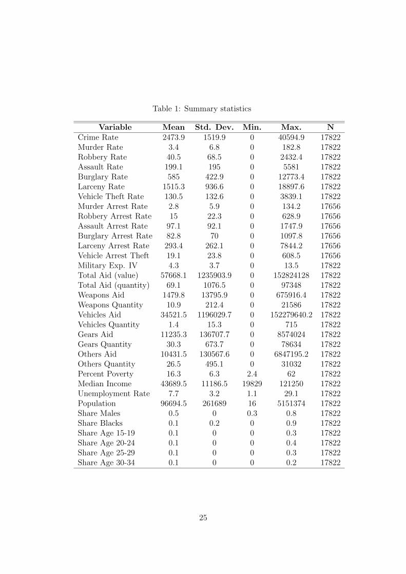
Table 1: Summary statistics

Variable Mean Std. Dev. Min. Max. NCrime Rate 2473.9 1519.9 0 40594.9 17822Murder Rate 3.4 6.8 0 182.8 17822Robbery Rate 40.5 68.5 0 2432.4 17822Assault Rate 199.1 195 0 5581 17822Burglary Rate 585 422.9 0 12773.4 17822Larceny Rate 1515.3 936.6 0 18897.6 17822Vehicle Theft Rate 130.5 132.6 0 3839.1 17822Murder Arrest Rate 2.8 5.9 0 134.2 17656Robbery Arrest Rate 15 22.3 0 628.9 17656Assault Arrest Rate 97.1 92.1 0 1747.9 17656Burglary Arrest Rate 82.8 70 0 1097.8 17656Larceny Arrest Rate 293.4 262.1 0 7844.2 17656Vehicle Arrest Theft 19.1 23.8 0 608.5 17656Military Exp. IV 4.3 3.7 0 13.5 17822Total Aid (value) 57668.1 1235903.9 0 152824128 17822Total Aid (quantity) 69.1 1076.5 0 97348 17822Weapons Aid 1479.8 13795.9 0 675916.4 17822Weapons Quantity 10.9 212.4 0 21586 17822Vehicles Aid 34521.5 1196029.7 0 152279640.2 17822Vehicles Quantity 1.4 15.3 0 715 17822Gears Aid 11235.3 136707.7 0 8574024 17822Gears Quantity 30.3 673.7 0 78634 17822Others Aid 10431.5 130567.6 0 6847195.2 17822Others Quantity 26.5 495.1 0 31032 17822Percent Poverty 16.3 6.3 2.4 62 17822Median Income 43689.5 11186.5 19829 121250 17822Unemployment Rate 7.7 3.2 1.1 29.1 17822Population 96694.5 261689 16 5151374 17822Share Males 0.5 0 0.3 0.8 17822Share Blacks 0.1 0.2 0 0.9 17822Share Age 15-19 0.1 0 0 0.3 17822Share Age 20-24 0.1 0 0 0.4 17822Share Age 25-29 0.1 0 0 0.3 17822Share Age 30-34 0.1 0 0 0.2 17822

25

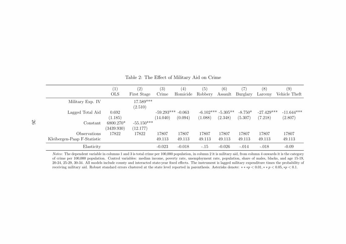
Table 2: The Effect of Military Aid on Crime

(1) (2) (3) (4) (5) (6) (7) (8) (9)OLS First Stage Crime Homicide Robbery Assault Burglary Larceny Vehicle Theft

Military Exp. IV 17.589***(2.510)

Lagged Total Aid 0.692 -59.293*** -0.063 -6.102*** -5.305** -8.750* -27.429*** -11.644***(1.185) (14.040) (0.094) (1.088) (2.348) (5.307) (7.218) (2.807)

Constant 6800.270* -55.150***(3439.930) (12.177)

Observations 17822 17822 17807 17807 17807 17807 17807 17807 17807Kleibergen-Paap F-Statistic 49.113 49.113 49.113 49.113 49.113 49.113 49.113

Elasticity -0.023 -0.018 -.15 -0.026 -.014 -.018 -0.09

Notes: The dependent variable in columns 1 and 3 is total crime per 100,000 population, in column 2 it is military aid, from column 4 onwards it is the categoryof crime per 100,000 population. Control variables: median income, poverty rate, unemployment rate, population, share of males, blacks, and age 15-19,20-24, 25-29, 30-34. All models include county and interacted state-year fixed effects. The instrument is lagged military expenditure times the probability ofreceiving military aid. Robust standard errors clustered at the state level reported in parenthesis. Asterisks denote: ∗ ∗ ∗p < 0.01, ∗ ∗ p < 0.05, ∗p < 0.1.

26

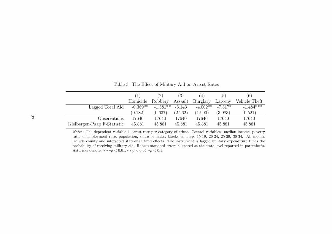
Table 3: The Effect of Military Aid on Arrest Rates

(1) (2) (3) (4) (5) (6)Homicide Robbery Assault Burglary Larceny Vehicle Theft

Lagged Total Aid -0.389** -1.581** -3.143 -4.002** -7.317* -1.484***(0.182) (0.637) (2.262) (1.900) (3.983) (0.521)

Observations 17640 17640 17640 17640 17640 17640Kleibergen-Paap F-Statistic 45.881 45.881 45.881 45.881 45.881 45.881

Notes: The dependent variable is arrest rate per category of crime. Control variables: median income, povertyrate, unemployment rate, population, share of males, blacks, and age 15-19, 20-24, 25-29, 30-34. All modelsinclude county and interacted state-year fixed effects. The instrument is lagged military expenditure times theprobability of receiving military aid. Robust standard errors clustered at the state level reported in parenthesis.Asterisks denote: ∗ ∗ ∗p < 0.01, ∗ ∗ p < 0.05, ∗p < 0.1.

27

Table 4: The Effect of Military Aid on Police Activities

(1) (2) (3) (4) (5) (6) (7) (8)Civilian Officers to Civil Disorder Offenders Citizen

Officers Employees Employees Ratio Calls Injuries Assaults Killed Complaints

Lagged Total Aid -0.405* -2.368** 0.001 -0.185 -0.063 -0.003 -0.010 -0.085(0.227) (0.966) (0.001) (0.195) (0.048) (0.005) (0.032) (0.081)

Observations 148691 148691 119069 148691 148691 148691 16605 516KP F-Statistic 11.494 11.494 10.626 11.494 11.494 11.494 9.634 2.384

Notes: The dependent variable is the numbers of officers (column 1), of civilian employees (column 2), their ratio (column 3), the number ofcalls (column 4), injuries (column 5), assaults (column 6) on the police, the number of offenders killed (column 7) and the number of citizencomplains (column 8). Control variables: median income, poverty rate, unemployment rate, population, share of males, blacks, and age15-19, 20-24, 25-29, 30-34. All models include county and interacted state-year fixed effects. The instrument is lagged military expendituretimes the probability of receiving military aid. Robust standard errors clustered at the state level reported in parenthesis. “KP F-Statistic”stands for Kleibergen-Paap F-Statistic. Asterisks denote: ∗ ∗ ∗p < 0.01, ∗ ∗ p < 0.05, ∗p < 0.1.

28