July 1, 1987

FROM MOUSE TO MAN:THE QUANTITATIVE ASSESSMENT

OF CANCER RISKS

by

D A FreedmanDepartment of StatisticsUniversity of California

Berkeley, Ca 94720415-642-2781

H ZeiselLaw School

University of ChicagoChicago, Ill 60637

312-702-9494

Technical Report No. 79Department of StatisticsUniversity of California

Berkeley, Ca 94720

To appear inStatistical Science

Summary

Results from animal experiments are often used to assess cancerrisks to humans from low doses of chemicals. This involves twoextrapolations: from high dose to low dose, and from animals tohumans. This paper will review the logic of both.

In general, absent other information, we think that a chemicalwhich is carcinogenic in a well-run animal experiment should beviewed with some suspicion. However, there are real problemswith most animal experiments as they are currently done, andthere are serious inconsistencies in the results. One probablecause is poorly defined endpoints, and another is uncontrolledvariation. A number of suggestions are made for improvement,including proper randomization, 'blinding' the necropsy work, anduse of statistical techniques appropriate to multiple endpoints.

Numerical assessments of human risk, even if based on good animaldata, seem well beyond the scope of the scientifically possible.Thare are substantial differences in sensitivity between species,stranS,sexes, and individuals. Experimental work is needed,to quantify these differences and explore their biological bases.

The dose-response models now used in numerical extrapolationare quite far removed from the biology. At present there seemsto be no sound way to choose a model on either biological orSLatLstical grounds, and different models give substantiallydifferent risk estimates. On this score, there is little hopefor progress until the biology of cancer is better understood.

The paper is organized as follows. The issties are set out inthe first section. Then the one-hit model is introduced in thecontext of a stylized risk assessment for DDT. Next the maingeneralizations of the one-hit model are explained: the multi-hit, Weibull, and multi-stage. The biological foundations forthese models are reviewed, and the impact of model selection onlow-dose risk estimates is stressed. Dose scales and biologi-cal scaling factors are discussed, and then the conventionalarguments for the mouse-to-man extrapolation. The DDT carcino-genes'is literature is surveyed, to show the quality of animalexperiments. Opinions by others are cited, and conclusions aredrawn.

Authors' footnote. Some of the work discussed in this paper was done white the authors were consultingfor the fire of Skadden, Arps, Slate, Meagher & Floe in a law suit about DDT contamination, ultiemtelysettled out of court. We would like to thank the following individuals for useful discussions, withoutimplying their agreement-- or disagreesent: J Bailar, P Diaconis, L Gold, L LeCae, S Moolgavkar, L Moses,D Petitti, M Pike, J Robins, S Swan, A Trersky, A Whittesore.

Table of Contents

1. Introduction 1

2. An example: the one-hit model 8

3. Other dose-response models 14Biological foundations for the multi-hit and Weibull 15The multi-stage model 18Fitting the models to animal data 20

4. Dose scales and the species extrapolation 25

5. The qualitative extrapolation 27The mammalian argument 27The mouse-to-rat argument 27The man-to-mouse argument 30Consistency with epidemiology 33

6. Review of carcinogenesis experiments 36

7. What do others 3ay? 45The Food Safety Council 45The IARC 46The OSTP 47The OTA 48The EPA 49The Saffiotti report 50The NAS 51Other authors 52

8. Conclusions 54Bioassays 54Qualitative extrapolation 54Quantitative extrapolation 55Policy implications 56

References 57

1

1. Introduction

New chemicals and some old ones must be tested for safety. Froman abstract scientific viewpoint, the best data would come fromcontrolled experiments. However, experiments on humans areethically permissible only rarely, so other kinds of evidencemust be brought to bear. In some cases, good epidemiologicalevidence is available, although such observational studies haveweaknesses of their own.

In most cases, no human data is available, and one turns toexperiments on animals., Even if these are flawlessly done, twoextrapolations are needed: from animals to humans, and from highdoses in the experiments to the relatively low occupational orenvironmental exposures of interest. Our main topic is thereliability of these extrapolations. Before stating thescientific issues more sharply, we would like to explaina bit more of the practical background.

Two kinds of health effects must be considered. Some chemicalsare acutely toxic in small doses. With others, exposure atordinary levels does not cause any immediate harm, but chronicexposure at low levels may create a serious health hazard. Inparticular, chronic exposure to some chemicals in the workplacesubstantially increases the risk of cancer; asbestos and vinylchloride are two prominent examples.

Cancer risks caused by chemicals are a matter of great publicconcern, because cancer is one of the most mysterious andfrightening of modern diseases. In the US today it accountsfor about one-fourth of all deaths. However, much controversysurrounds cancer statistics. Some commentators argue that thereis an explosive cancer epidemic caused by exposure to chemicals;this view seems to be widely held by the public, althoughcareful analysis of the available data does not lead tosuch alarming conclusions.

Crude cancer rates (not adJusted for age) have been going up,but this is mainly because of increased life expectancy: thereare more old people at risk for the disease. To make sensiblecomparisons, it is necessary to standardize for age. On thisbasis, lung cancer rates have indeed been going up, followingpast increases in cigarette smoking. (But see Doll & Peto 1981Appendix E or Franks & Teich 1986 p76 for evidence on a recentdown-turn explained by-changing smoking habits.)

2

Figure 1. Cancer death rates per 100,000, by site(age standardized to the 1970 population)

2 s

C 00*

a.4so USS*S.. .um m US 3?, sg?FiISSS.,

Source: ACS (1986). Rates are for both sexes combined except breastand uterus fesale population only and prostate male population only.Figure reproduced by courtesy of the American Cancer Society.

For other forms of cancer, the picture is quite mixed: forexample, stomach cancer and liver cancer have been going down,leukemia up; the reasons are not well understood. On balance,except for the lung, cancer rates have been nearly constant(figure 1). For discussion, see eg Bailar & Smith (1986),Cairns (1985), Doll & Peto (1981), Higginson (1979),Peto (1980), National Academy of Sciences (1975, 1983b).

Cancer epidemiology depends on nonexperimental studies ofhuman populations, with all the problems of confounding. Thelong periods of time between exposure and manifestation of cancerare a special complication: thus, asbestos workers from WorldWar II are still developing mesothelioma in the 1980s. Further-more, cancer seems to be inherently probabilistic: somenon-smokers do get lung cancer while many smokers avoidthis disease. Disentangling the causes of cancer in suchcircumstances is a very difficult exercise, but remarkableprogress has been made: see eg Franks & Teich (1986) for arecent review.

3

Public concern, and the obstacles facing epidemiology, explainthe heavy reliance on animal experiments. The Delaney amendmentto the Food, Drug, and Cosmetic Act of 1954 outlawed residues inprocessed foods of chemicals which caused a risk of cancerto animals or humans. Such zero-risk requirements can be inter-preted operationally as meaning "very low risk", where the risksare estimated from bioassays and extrapolated to humans. See,for example, National Academy of Sciences (1987).

Under prevailing standards, a good bioassay involves two speciesof test animals, typically rats and mice. Since cancer usuallydevelops late in life, both for animals and man, the test speciesmust have relatively sbort life-spans. Rats and mice live forabout two years. They are small, cheap, and easy to maintainunder lab conditions. Furthermore, experimentalists have muchexperience with rats and mice. There seem to be no other seriousarguments for using these two test species in cancer testing.(Cf eg the Office of Technology Assessment 1981 p126.)

The basic axiom of toxicology is that the dose makes the poison:anything (even water) is harmful in large-enough quantities.Administering the test chemical at too high a dose kills theanimals before they can develop cancer. Therefore, the experi-mental protocol requires the preliminary determination of theMTD, or maximally tolerated dose. By definition, above the MTDthere are signs of acute toxicity (eg, stunting of growth, dis-orientation, etc).

According to standard protocols, in the main part of theexperiment some animals are given the MTD, while others getspecified fractions of the MTD. Some animals get no dose atall-- the control group. A control group is needed because theanimals develop cancer spontaneously. Indeed, many strains ofinbred lab animals seem particularly vulnerable to this disease.The bioassay is therefore intrinsically statistical. The wholeidea is to compare the response of the test and control groups,to see if the incidence of cancer in the test group is above thechance level.

With three dose groups (eg, the MTD, half the MTD, zero), twosexes, and two test species, there are twelve groups of animals.It is conventional to start with 50 animals per group. So therewill be 600 animals on test. This seems like a fairly modestexperiment, but at the time of writing the cost is severalhundred thousand dollars. Larger experiments have been done,like the 'mega-mouse experiment'-with 24,000 animals on test,but these are clearly exceptional. (For some discussion of themega-mouse experiment, see Staffa & Mehlman 1980.) The economicsof bioassays dictate testing at the MTD. Indeed, with 800animals, there is little chance of observing small effects atlow doses, so the test would have negligible power at such doses.

4

Bioassays are used to make risk assessments, and then twoextrapolations are needed:

i) Numeric extrapolation, from high dose to low dose.

ii) Species extrapolation, from the test animals to humans.

The extrapolation from high dose to low will be based on sometype of mathematical model. The potential health hazards tohumans usually result from doses which are 10 or 100 or 1000times smaller than the experimental doses, so the extrapolationis over quite a range. How good are the dose-response models?What evidence validates them? These questions will be consideredin sections 2 and 3.

While there are many similarities between mice and men, there arealso many differences. What evidence shows the validity of thespecies extrapolation? Workers in the field call this issuethe mouse-to-man Problem. The statistical logic behind thisextrapolation will be reviewed in sections 4 and 5.

The quality of the bioassays as experiments will also beconsidered. Does a positive finding mean that the chemicalcauses cancer in the test species, or is this likely to be anartifact of the experimental design and analysis? Section 6reviews the DDT bioassays in an attempt to answer thesequestions.

Other literature is discussed in section 7, and conclusionsare given in section 8. The balance of this section considerssome of the public-policy issues, and some of the conventionalresponses to our sort of critique.

Cancer, and screening chemicals for carcinogenic hazards, is anexplosive topic. In such a context, asking questions is seenas a political act-- especially if the questions turn out tohave no satisfactory answers. (The interplay between the scienceand the politics is fascinating; see for example Epstein 1979 andEfron 1984.)

5

Some of the work on this essay was prompted by a consultingengagement with lawyers for a DDT manufacturer. The latter wassued by persons claiming damage from toxic wastes. The case wassettled out of court, so there seems to be no reason to name theparties. Before working on the case, we felt-- along with everyother educated person-- that DDT caused cancer. On review, theunderlying evidence for this proposition turned out to be quiteflimsy.

The contrast between the weakness of the evidence on DDT and thestrength of the naive convictions is one motive for writing thisessay, and DDT is used to illustrate the difficulties in riskassessment. The increasing use of risk models in the nation'slaw courts and government regulatory agencies, and our skepticismabout the scientific foundations of the enterprise, explains theurgency we feel about the issue.

We do not wish to be understood as opposing government regula-tion of chemicals, or favoring uncontrolled pollution of theenvironment. Nor are we arguing against animal experiments.Great science has been done in the field of chemical carcino-genesis, and much animal work remains to be done if thebiology of cancer is to be understood. However, routinebioassays have little to do with basic research, nor do they(in our opinion at least) contribute much to the scientificregulation of health or environmental hazards.

6

Any critique of the regulatory process generates two conventionalresponses. The first is that the human costs of introducinga carcinogen into the environment could be staggering, so anydoubts should be resolved in favor of regulation. This may beright for food coloring, but the argument for a chemical likeDDT is not so easy. Indeed, suppose the evidence for carcino-genicity of DDT in humans is weak, but DDT is a cheap, effectiveinsecticide widely used in agriculture and for the control ofdiseases spread by insects (such as malaria). Finally, supposethat DDT is not especially toxic to humans, while the availablereplacements are not orny more expensive, but also substantiallymore toxic.

Given these hypotheses, the balance of the costs in banning DDTis not so clear. On the one hand, DDT is clearly harmful towild-life, and may pose some long-term hazard to humans. On theother hand, banning DDT may reduce the supply of food, increasethe risks from malaria, and cause fatalities among insecticideworkers: see Wald and Doll (1985, esp p119). An informedevaluation of the strength of the evidence for thecarcinogenicity of DDT becomes crucial.

7

A second conventional response to our sort of critique: Theexisting technology for risk assessment may not be perfect, butit is better than nothing, and there is no replacement technologyin sight. This argument is fine in some contexts. Engineers,for example, do know how to build roads. Therefore, someone whocriticizes the plan for a road can quite reasonably be asked toproduce a better plan.

With intellectual technologies like dose-response modeling(or the computer progragming for Star Wars, to take an examplewith a different political flavor) the situation is quitedifferent. Then the whole question is whether any technologycan do the Job. It may be worthwhile to face this questionsquarely. Indeed, the limits to knowledge may themselves beworth knowing; at least there is some precedent for takingsuch a position.

A final comment on the nothing-is-perfect argument. Dose-response models are imperfect. Nor was the maiden voyage of theTitanic a great success. Such understatements conceal more thanthey reveal. There are degrees of imperfection in theoriesranging from quantum mechanics to astrology. The presentessay attempts to locate risk assessment somewhare alongthis spectrum.

For a spirited defense of risk assessment (and only in part as alesser evil), see eg Crouch & Wilson (1987), Lave (1987), orRussell & Gruber (1987).

8

2. An example: the one-hit model

A stylized account of a risk assessment involving DDT providesa useful starting point, and serves to introduce the one-hitmodel (the rationale for the name will be explained below).The obJect of the analysis was to estimate the risk of cancercaused by DDT contamination. Levels of contamination wereestimated for individual plaintiffs in a lawsuit, and rangedfrom 1 to 30 parts per million (ppm) in the diet. This mayseem low, but usual DDT levels run at parts per billion.

U

In the law case, the focus was on two metabolites of DDT,namely DDD and DDE. For now, the three substances can beconsidered together. To fix ideas, suppose an analyst wants toestimate the risk of cancer due to DDT at 20 ppm in the diet. Agood data base for the purpose would show cancer rates for twosimilar human populations, one exposed at levels around 20 ppmand the other exposed at much lower levels. Any difference inthe two cancer rates might be attributed to the difference in DDTexposures, subject to the usual arguments about interpretingobservational data. For most risk assessments, including the oneunder discussion, such data do not exist.

At this juncture, risk assessment turns to animal data. To focuson essentials, suppose that lifetime exposure to DDT at 20 ppm inthe diet causes an extra cancer risk of 10% in lab mice. Thiswill be extrapolated to people, and background cancer rates mustbe considered. In round numbers, about 25% of the populationof the US dies of cancer. Now a crucial step: if people arethen exposed to 20 ppm of DDT for their lifetimes, their cancerrate are assumed to go up to

25% + 10% of (100% - 25%) 32.5%

The first term represents the background cancer rate. The secondterm on the left represents the effect of DDT. The 10% has beenextrapolated from mice to humans. That is the species extrapo-lation. (For official guidelines on this extrapolation, seeeg US Environmental Protection Agency 1986; for a sympatheticpresentation of examples, see eg Crouch & Wilson 1987.)

9

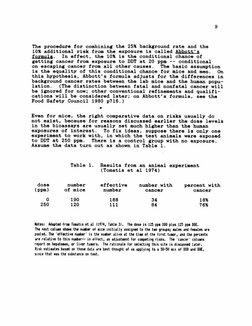
The procedure for combining the 25% background rate and the10% additional risk from the exposure is called Abbot&'formula. In effect, the 10% is the conditional chance ofgetting cancer from exposure to DDT at 20 ppm -- conditionalon escaping cancer from all other causes. The basic assumptionis the equality of this conditional chance for mice and men. Onthis hypothesis, Abbott's formula adjusts for the differences inbackground cancer rates between the lab mice and the human popu-lation. (The distinction between fatal and nonfatal cancer willbe ignored for now; other conventional refinements and qualifi-cations will be considered later; on Abbott's formula, see theFood Safety Council 1980 p716.)

Even for mice, the right comparative data on risks usually donot exist, because for reasons discussed earlier the dose levelsin the bioassays are usually set much higher than the humanexposures of interest. To fix ideas, suppose there is only oneexperiment to work with, in which the test animals were exposedto DDT at 250 ppm. There is a control group with no exposure.Assume the data turn out as shown in Table 1.

Table 1. Results from an animal experiment(Tomatis et al 1974)

dose number effective number with percent with(ppm) of mice number cancer cancer

0 190 188 34 18%250 120 111 84 76%

Notes: Adapted from Tomatis et al (1974, Table 3). The dose is 125 ppe DDD plus 125 ppe DOE.The next column shows the number of sice initially assigned to the two groups; males and females arepooled. The 'effective number' is the number alive at the time of the first tumor, and the percentsare relative to this number-- in effect, an adjustment for competing risks. The 'cancer' columnsreport on hepatomas, or liver tumors. The rationale for selecting this site is discussed later.Risk estimates based on these data are best thought of as applying to a 50-50 mix of DDD and DDE,since that was the substance an test.

10

Given that a mouse escapes cancer from other causes, itsconditional chance of developing cancer from the DDT exposureis estimated (in effect, from Abbott's formula run backwards) as

(76 - 18)/(100 - 18) = 71%

The exposure, however, is at 250 ppm; the analyst must extrapo-late the risk down to 20 ppm, for the mice. This is the numericextrapolation. After the risk at 20 ppm is estimated for themice, the same estimate is used for people; this is the speciesextrapolation described above.

U

Numeric extrapolation involves a dose-response model whichpredicts response (chance of cancer) from dose (ppm in thediet). The formula will have one or more parameters which mustbe estimated from the data. There are many formulas to chosefrom, including the one-hit model and its generalizations likethe multi-hit, the Weibull, and the multi-stage. Thesegeneralizations will be described below. For now, the focusis the one-hit model.

The basic equation in the one-hit model involves P(d), the totallifetime chance of getting cancer at dose level d. Thus, P(0)is the chance for the control animals, whose dose is zero. AndP(250) is the chance for animals fed 250 ppm. These chancescan be estimated by the fractions observed in the experiment.

The one-hit model involves the parameter k, which is called'potency'. The basic equation can now be presented:

(1) P(d) = P(O) + [1 - P(O)] x [1 - e-kd]

The left side of equation represents the total chance of cancer,at dose d-- due to the exposure and to all other causes.

11

On the right side of equation (1):

P(O) represents the background chance of getting cancerdue to all other causes-- at zero dose of thechemical on test

1 - P(O) represents the chance of escaping cancer from allthese other causes.

1 - e-kd gives the chance of getting cancer due to theexposure, at dose d-- conditional on escaping cancerfrom the otsher causes.

Technically, the one-hit model is the formula 1 - e-kd for theconditional chance. In equation (1), this has been combined withthe background chance P(O).

For fixed dose d, as k goes up the predicted chance of cancergoes up (hence the name, potency). Keeping the potency fixed,when the dose goes up the predicted chance of cancer goes uptoo, as is only reasonable. When the dose gets large, thechance of cancer approaches 1.0, or certainty. (This seemsless reasonable, and with eg vinyl chloride or 2-AAF, theresponse rate in bioassays at high doses is substantiallyless than 100%.)

Now a minor technical fact: If kd-- the product of potency anddose-- is small, the equation is essentially

(2) P(d) = P(O) + [1 - P(O)] x kd

Hence, the model is sometimes called 'linear'.

12

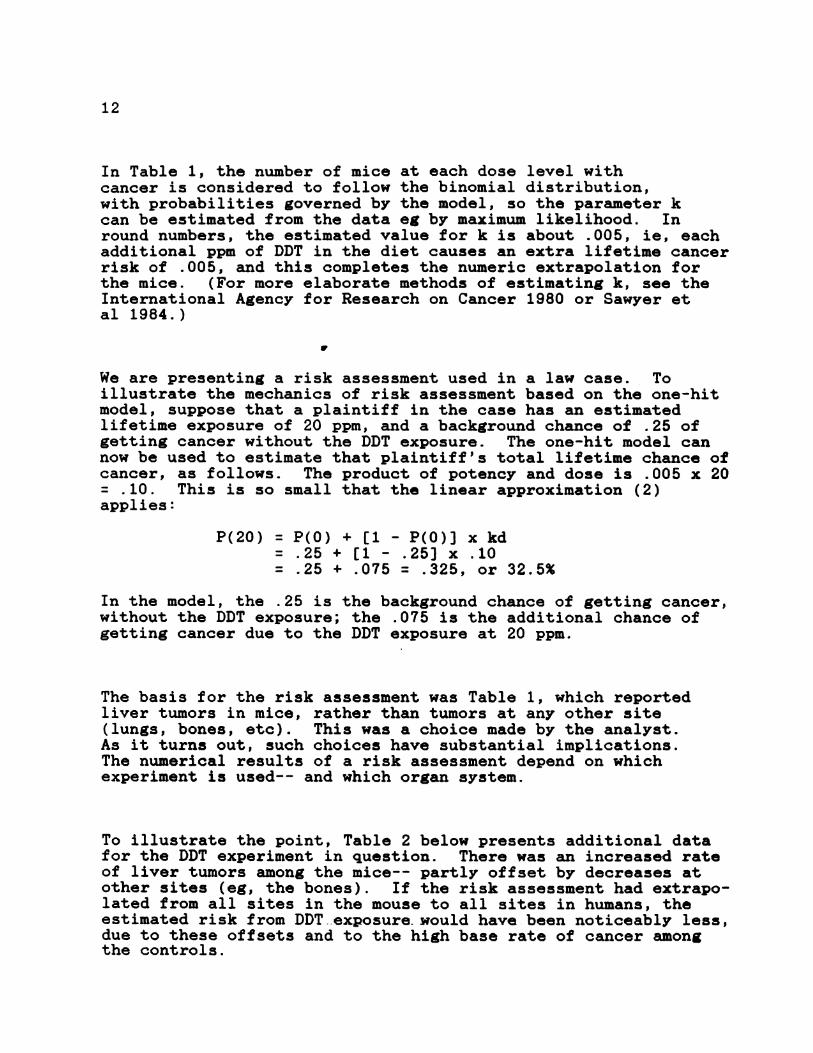
In Table 1, the number of mice at each dose level withcancer is considered to follow the binomial distribution,with probabilities governed by the model, so the parameter kcan be estimated from the data eg by maximum likelihood. Inround numbers, the estimated value for k is about .005, ie, eachadditional ppm of DDT in the diet causes an extra lifetime cancerrisk of .005, and this completes the numeric extrapolation forthe mice. (For more elaborate methods of estimating k, see theInternational Agency for Research on Cancer 1980 or Sawyer etal 1984.)

We are presenting a risk assessment used in a law case. Toillustrate the mechanics of risk assessment based on the one-hitmodel, suppose that a plaintiff in the case has an estimatedlifetime exposure of 20 ppm, and a background chance of .25 ofgetting cancer without the DDT exposure. The one-hit model cannow be used to estimate that plaintiff's total lifetime chance ofcancer, as follows. The product of potency and dose is .005 x 20= .10. This is so small that the linear approximation (2)applies:

P(20) = P(0) + [l - P(0)] x kd= .25 + tl - .25] x .10= .25 + .075 = .325, or 32.5%

In the model, the .25 is the background chance of getting cancer,without the DDT exposure; the .075 is the additional chance ofgetting cancer due to the DDT exposure at 20 ppm.

The basis for the risk assessment was Table 1, which reportedliver tumors in mice, rather than tumors at any other site(lungs, bones, etc). This was a choice made by the analyst.As it turns out, such choices have substantial implications.The numerical results of a risk assessment depend on whichexperiment is used-- and which organ system.

To illustrate the point, Table 2 below presents additional datafor the DDT experiment in question. There was an increased rateof liver tumors among the mice-- partly offset by decreases atother sites (eg, the bones). If the risk assessment had extrapo-lated from all sites in the mouse to all sites in humans, theestimated risk from DDT-exposure would have been noticeably less,due to these offsets and to the high base rate of cancer amongthe controls.

13

Table 2. Results from Tomatis et al (1974). Maleand female mice combined. Rates for alltumors and for liver tumors.

All tumors Liver tumors

Controls 89% 18%250 ppm DDD 93% 27%250 ppm DDE 91% 86%125 ppm DDD + 125 ppm;DDE 93% 76%

Note: The base of the percentage is the 'effective number', ie, the number of animals alive at the timeof the first tumor observed. Table I reported the percentage of liver twors for the controls and for thedose group 125 ppm DDD + 125 ppm DDE.

The estimated risk would also be much less if the extrapola-tion were from liver cancer in mice to liver cancer in people.Indeed, liver cancer is quite rare in the US. So P(0) inequation (1) for people would be much less. (Despite theincrease in chemical pollution and the impact of chemicalson the mouse liver, the incidence rate of liver cancer inthe US has been decreasing since the 1930s, as shown inFigure 1 above.)

The risk assessment also depends on assuming the formula (1) formice and for humans, with the equality of k for the two species.The merits of all these assumptions will be considered below:but first, some of the main generalizations of the one-hit modelfor low-dose risk extrapolation will be discussed.

14

3. Other dose-response models

There are many dose-response models, ie, equations which predictresponse from dose and are used to extrapolate from high doseto low. The one-hit model and three generalizations will bereviewed, with some remarks on their biological foundations.(There are still other models which will not be reviewed, suchas Cornfield's 1977 hockey-stick model, or the Koolgavkar-Day-Stevens 1980 two-stage model. Although more realistic onbiological grounds, these models are seldom used in riskassessment. For a mathematical discussion of the various models,see Kalbfleisch-Krewski-van Ryzin 1983. Also see Moolgavkar 1986for a review of the evidence on his model.)

As will be seen, the one-hit model does not fit typical data setsfrom animal experiments. The multi-hit, Weibull and multi-stageall tend to fit reasonably well, but lead to very differentrisk estimates at low doses. The biological foundations for allthe models are quite weak, so there is no sound way to choose onerather than another, and no way to make reliable low-dose riskestimates.

The eguations

First, the equations for the various models: let Q(d) bethe chance of getting cancer at dose level d, due to theexposure, ie, conditional on escaping cancer from other causes.(Abbott's formula is used to bring in the latter.) As theequations show, the one-hit model is a special case of themulti-hit, Weibull, or multi-stage, since (4-6) specializeto (3) on setting m=1.

The one-hit, with parameter k:

(3) Q(d) = 1 - exp(-kd)

The multi-hit, with parameters k and m:kA

(4) Q(d) f tin-I exp(-t) dt/I(m)0

15

The Weibull, with parameters k and m:

(5) Q(d) = 1 - exp(-kdm)

The multi-stage, with m stages sensitive and linear response ateach stage:

(6) Q(d) = 1 - exp(-Z aidi)

(This formula is a convpntional approximation; the model will beexplained in more detail below.)

Biological foundations for the multi-hit and Weibull

The multi-hit equation (4), for integer values of m, can bederived by assuming that 'hits' follow a Poisson process withparameter kd, and a cell becomes malignant when it suffers mhits. (The one-hit model requires only one hit, explaining thename.) However, these assumptions constitute a fable rather thana serious model, since there does not seem to be any precisebiological definition for a 'hit', with some evidence that aspecific number of hits causes cancer, or that hits followa Poisson process.

The multi-hit (and Weibull) equations can also be derived byassuming that each individual in the population has a threshold,and gets cancer if the dose exceeds that threshold. Appropriatechoice of the distribution for the thresholds leads to the equa-tion of the model: gamma distributions give the multi-hit;extreme-value distributions, the Weibull. (In applications,m in the multi-hit model is often taken to be real rather thaninteger, so the 'hit' idea is not germane but the thresholdidea still applies.)

Of course, the threshold hypothesis is open to some dispute. Andthere is no good reason why the distribution of thresholds shouldfollow the extreme-value or gamma-- or any other textbook case.

16

The multi-staae model

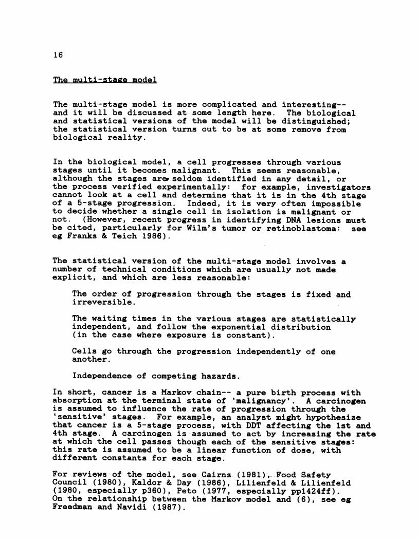
The multi-stage model is more complicated and interesting--and it will be discussed at some length here. The biologicaland statistical versions of the model will be distinguished;the statistical version turns out to be at some remove frombiological reality.

In the biological model, a cell progresses through variousstages until it becomes malignant. This seems reasonable,although the stages are seldom identified in any detail, orthe process verified experimentally: for example, investigatorscannot look at a cell and determine that it is in the 4th stageof a 5-stage progression. Indeed, it is very often impossibleto decide whether a single cell in isolation is malignant ornot. (However, recent progress in identifying DNA lesions mustbe cited, particularly for Wilm's tumor or retinoblastoma: seeeg Franks & Teich 1986).

The statistical version of the multi-stage model involves anumber of technical conditions which are usually not madeexplicit, and which are less reasonable:

The order of progression through the stages is fixed andirreversible.

The waiting times in the various stages are statisticallyindependent, and follow the exponential distribution(in the case where exposure is constant).

Cells go through the progression independently of oneanother.

Independence of competing hazards.

In short, cancer is a Markov chain-- a pure birth process withabsorption at the terminal state of 'malignancy'. A carcinogenis assumed to influence the rate of progression through the'sensitive' stages. For example, an analyst might hypothesizethat cancer is a 5-stage process, with DDT affecting the lst and4th stage. A carcinogen is assumed to act by increasing the rateat which the cell passes though each of the sensitive stages:this rate is assumed to be a linear function of dose, withdifferent constants for each stage.

For reviews of the model, see Cairns.(1981), Food SafetyCouncil (1980), Kaldor & Day (1986), Lilienfeld & Lilienfeld(1980, especially p360), Peto (1977, especially ppl424ff).On the relationship between the Markov model and (6), see egFreedman and Navidi (1987).

17

There are two kinds of evidence in favor of the model, human andanimal. The main human evidence is as follows. For many kindsof cancer, the age-specific incidence is approximately a power ofage: algebraically,

incidence at age t = constant x tP

This pattern is predicted by the model. More precisely, Armitageand Doll (1961) developed the model to explain this power law.In the model, the power p is related to the number of stages,which usually turns out to be between 4 and 6. See Peto (1977).

On the other hand, most cancers do not seem to follow the powerlaw: see eg Cook-Doll-Fellingham (1969), Lilienfeld & Lilienfeld(1980, esp p360). Kaldor & Day (1986, sec III) discuss some ofthe difficulties in making such analyses. Pike (1983) givesan example of how anomalies might be resolved, at least forbreast cancer; and Moolgavkar-Day-Stevens (1980) in effect givea counter-argument to that sort of resolution, by showing howtheir model, which is quite different, also fits that data.

Lung cancer may be the best studied, and is usually thought tofollow the multi-stage model quite well: see Doll & Peto (1978).However, recent analyses of the data shows serious discrepancieseven there: Freedman & Navidi (1987), also see Brown & Chu (1986).In brief, a variety of multi-stage models will fit the originalDoll & Peto data for current smokers. No model fits the Dornveterans cohort, or the American Cancer Society volunteers.

Turn now to the animal evidence on 'initiation' and 'promotion'.The idea is that an initiator causes a cell to change from itsnormal state to a pre-malignant state, in which it may remainindefinitely; a promoter causes an initiated cell to becomecancerous. (Some writers consider a third stage of proliferation;others subdivide the promotion stage: see eg InternationalAgency for Research on Cancer 1984.) Only one typical exampleneed be given. DMBA (dimethylbenzanthracene) is consideredan initiator, croton oil (more specifically, its phorbol esterconstituent) a promoter. The reason: Applying the agents inthe order

DMBA first, croton oil second

produces a large yield of tumors, mainly non-malignantpapillomas. Applying them in the reverse order or separatelygives a much smaller yield: see eg Boutwell (1964).

18

In the framework of the multi-stage model, an initiator isheld to affect the rate of progression through an early stage; apromoter affects a late stage. Some 'complete' carcinogens arethought to be both promoters and initiators-- cigarette smoke,for example.

Now, some of the problems. These experiments relate to theprogression of tumors-- colonies of cells: the mathematicalmodel relates to the progression of an individual cell. Cellswithin a tumor become remarkably heterogeneous in their geneticmakeup, so progression of the tumor is not good evidence aboutthe progression of individual cells.

V

Even at the level of whole tumors, there are interesting newexperiments which show that for some initiators and promoters.thesequence

initiator, promoter, initiator

produces a much larger yield of malignancies than the sequence

initiator, promoter

Likewise, the order

promoter, initiator, promoter

increases the tumor yield. This is not easy to reconcile withthe conventional view of initiation and promotion. See Henningset al (1983), and for a review International Agency for Researchon Ccancer (1984). The phenomenon was predicted on theoreticalgrounds by Moolgavkar & Knudson (1981).

Moreover, with typical initiator-promoter protocols, only oneapplication of the initiator is needed. And the timing of thesuccessive applications of the promoter is critical: if theapplications are too far apart, or too close together, the effectdisappears (Boutwell 1984). These facts cut against the model.

The idea of reversibility presents serious problems for themodel, too. There is now much evidence for the reversibilityof some lesions, including papillomas; the fixed order ofprogression through the stages of the model then comes intoquestion. See eg Cohen et al (1984, esp p103), Slaga (1983);for reviews, Montesano-Bartsch-Tomatis (1980), Office ofScience and Technology Policy (1985, chap 1, sec V), UKDepartment of Health and Social Security (1981).

19

The idea of 'epigenetic' cancer is also incompatible with themodel: 'genetic' cancer is caused by damage to DNA, the geneticmaterial of the cell; 'epigenetic' cancer is caused by somefailure of surrounding tissue to regulate growth and differenti-ation, and this will affect all cells in the vicinity, contraryto the independence assumption in the model. For reviews, seeDouglas (1984), Franks & Teich (1986), Rubin (1980), the UKDepartment of Health and Social Security (1981). For reports onexperiments, see eg Stott et al (1981), Williams (1980, 1983).

Likewise, aging affects metabolic processes and may affectsusceptibility to cancer; this would contradict the model'sassumption of constant rates of progression. There is animalevidence (Peto et al 1975) to show that incidence of tumorsdepends on time since exposure rather than age, but there isalso evidence going the other way. For reviews, see Likhachev-Anisimov-Montesano (1985); or Sohal-Birnbaum-Cutler (1985)on the molecular biology of aging.

Another difficulty: while some carcinogens act in synergy,there are antagonistic pairs. See eg Richardson-Stier-Borsos-Nachtnebel (1952), Miller-Miller-Brown (1952). Okey (1972)shows that DDT protects female rats against the induction ofbreast cancer by DMBA. Cohen et al (1979) demonstrates aprotective effect from dioxin. A striking recent study showsthat aspirin increases the effect of the carcinogen FANFT at onesite but inhibits it at another-- Murasaki et al (1984). For areview of such interactions, see DiGiovanni et al (1980) orShankel et al (1986). The phenomenon is well outside the scopeof the model.

At this point, it may be useful to recall the distinction betweenthe biological and statistical versions of the multi-stage model.In the biological version, a colony of cells progresses throughstages on the way to cancer. In the statistical version of themodel, an individual cell executes a Markov chain through a fixedorder of states along the way to cancer, the transition ratesbeing linear functions of dose: these are hypotheses largelyabout unobservable entities. The statistical model may lead tobeautiful mathematics, and may have real heuristic power. Butit is much more loosely coupled to reality than the biologicalmodel. The statistical model-- the relevant one for quantitativerisk assessment-- is at a considerable distance from the realm ofscientific fact.

20

F'itting-the models to animal-data

The biological foundations for all the models seem to be quitespeculative, so there is no sound way to chose one over anotheron theoretical grounds. But the different models have verydifferent implications for risk assessment. As will be seen,the one-hit model does not fit typical data sets from animalexperiments: the multi-hit, Weibull and multi-stage all tend tofit reasonably well, but disagree by many orders of magnitude onthe estimates of risk at low doses.

V

There is an excellent review of the models and data sets byThe Scientific Committee of the Food Safety Council (1980). With14 data sets, the one-hit model is rejected 6 times (P < .05 bychi-squared); the multi-stage model is rejected once; the Weibulland multi-hit fit all the data sets. In 10 out of 14 cases, theWeibull and multi-hit offer significant improvements over theone-hit. In this context, the chi-squared test does not havemuch power, so rejection is a strong signal. For a morerecent review, with similar conclusions, see Hoel & Portier(1987).

In essence, the one-hit model is linear at low dose, and thislinearity is often contra-indicated by the data. The othermodels are sufficiently flexible to fit typical dose-responsedata. Since there are at most 6 dose groups in the Food SafetyCouncil data sets, this is perhaps not such a strict test. Fewanimal data sets have as many as 6 dose groups, so power todifferentiate among the models is low. With time-to-tumor data,the multi-hit model may not fare so well. Also see Carlborg(1981ab), who argues for the Weibull over the multi-stage inthe mega-mouse experiment.

For the purposes of risk assessment, it is a crucial point thatmany models will fit most of the data, while the choice of modelhas a profound impact on the estimated risks at the low doses ofinterest. In general, the one-hit model gives the highest riskestimates, and the multi-hit gives the lowest-- by quite largefactors. A few examples may be of interest: see Table 3. Foreg aflatoxin, the one-hit model gives 30 times the risk estimatedfrom the multi-stage, 1000 times the risk from the Weibull, and-40,000 times the risk from the multi-hit. The results in Table 3are not unusual. See, for example, Hoel-Kaplan-Anderson (1983),Krewski & van Ryzin (1981), Rai & van Ryzin (1979, 1981).

21

Table 3. The impact of the model onlow-dose risk estimates

multi- multi-substance one-hit stage Weibull hit

Aflatoxin 1 30 1000 40,000Dioxin 1 400 400 800

DMNA 1 700 700 2,700Dieldrin 1 3 200 1,000

DDT 1 2 70 200

Notes. From Food Safety Council (1980, Table 4). The 'Virtually Safe Dose', or VSD, is estimated fromeach of the four models, as that dose giving a risk of one in a silliom. The colum for the multi-stagemodel shoNs the ratio of its estimated VSD to the VSD estimated from the one-hit, for each of the 5substances. Likewise for the Weibull and the multi-hit.

Saccharin is another example of some interest. Published riskestimates, starting from the same animal data but using variousmodels, differ by factors of over 5,000,000. See the NationalAcademy of Sciences (1978, p3-72 for the data and pp3-61ff fordiscussion).

A final example is Haseman & Hoel's (1979) study of riskestimates derived from animal experiments on DDT. In all cases,the multi-stage model was used. With 8 studies and two sexes,there were 16 sub-experiments. For lung tumors there were 11cases where the risk estimate was zero: in the remaining 5cases, the risk estimates varied by factors up to 1000. Forliver tumors, as Haseman & Hoel remark, "the agreement wasbetter:" there was only one case where the risk estimate waszero, and in the remaining cases the variation was only by afactor of 250.

22

The artificiality of the models, and the sensitivity of theresults to the modeling assumptions, show how far removedrisk assessment is from an objective science. Indeed, the FoodSafety Council (1980, p718) quotes the Commissioner of the Foodand Drug Administration as follows:

The Commissioner has extensively reviewed the known procedures thatmay be used to derive an operational definition of the non-residuestandard of the act from animal carcinogenesis data. This review haspersuaded him that the same scientific and technological limitationsare common to all. Specifically, because the mechanism of chemicalcarcinogenesis is not understood, none of these procedures has afully adequate biological rationale. All require extrapolation ofrisk-level relations from responses in the observable range to thatarea of the dose-response curve where the responses are not obser-vable. Matters are further complicated by the fact that the risk-level relations adopted by the various procedures are practicallyindistinguishable in the observable range of risk (5 percent to 95percent) but diverge substantially in their projection of risks inthe non-observable range.

Why is low-dose extrapolation so difficult? The Commissionerexplained the answer quite clearly: Not enough is known aboutthe biological mechanisms of cancer. In fact, there are some 200different kinds of cancer, classified by site and tissue, withmany different biological mechanisms. Although much has beenlearned about the biology in the past few decades, many crucialdetails remain to be elucidated. In this light, any attempt todevelop one simple mathematical formula to describe cancer risksseems naive.

23

Some of the biological complexities in low-dose risk ex-trapolation should be mentioned explicitly-- eg, the role ofmetabolic pathways, genetics, repair mechanisms. For example,high doses may overwhelm repair mechanisms or metabolic pathwaysleading to detoxification: see Hoel-Kaplan-Anderson (1983) forthe impact on risk modeling, or Whittemore-Grosser-Silvers(1986); and for a review, Office of Science and TechnologyPolicy (1985, esp sec 3IIB).

V

Another example. Repeated injury to body tissue may increase therisk of cancer: the cells proliferate to repair the injury, andif the insult continues, this could increase the chance ofmistakes in DNA replication, leading in the end to heritablemutations. For some of the relevant animal experiments, seeMirsalis et al (1985), Moore et al (1982), Stott et al (1981).For reviews and discussion of the implications for models ofcarcinogenesis, see Ames-Magaw-Gold (1987, pp275-6), Farber(1984) or Iversen & Astrup (1984). For a different opinion,see Ward (1984).

The human liver is quite vulnerable to repeated insults: seeeg Bloom & Fawcett (1962, pp600ff) or Weinbren (1978, esp pp1207& 1243-1262). Consider alcohol: at high doses, it causes cir-rhosis of the liver by cell-killing and subsequent proliferation;at low or moderate doses, this does not occur. Likewise for ace-taminophen, the active ingredient in many pain-killers. Forthese substances, low-dose extrapolation on cirrhosis would bea scientific blunder, and we are not aware of attempts in thatdirection.

24

On the other hand, in bioassays many animal carcinogens likeDDT seem to affect the mouse liver through cell-killing athigh doses. And there certainly are attempts at low-dose riskassessment for such substances, even though the cell-killingmechanism is unlikely to operate at low doses.

(At sites other than the liver, acetaminophen seems to be weaklycarcinogenic by a different mechanism, while alcohol has a potentsynergistic effect with tobacco. Risk assessment at these siteswould run into serious problems too: see Doll & Peto, 1981,p1225 on alcohol; and International Agency for Research onCancer 1982 p17 on phenacetin, of which acetaminophen is theactive metabolite.)

To sum up, the choice of models has a decisive impact on low-dose risk estimates, and in the present state of knowledgethere is no sound way to pick one model rather than another.All except the one-hit will fit typical dose-response data sets,and none have adequate biological foundations. That is whyreliable estimates of risks at low dose cannot be made on thebasis of present knowledge. This completes the discussion ofextrapolation from high dose to low; turn now to the speciesextrapolation.

25

4. Dose scales and the species extrapolation

What is the basis for the species extrapolation? First, thedefinition of dose must be considered in more detail: Indeed,even granting that a man is Just a big mouse, one milligram ofDDT cannot mean the same thing for both of them, due to thedifference in size. However, there turn out to be many differentways to measure this difference. For example, a man weighs 2800times as much as a mouse, eats 300 times as much per day, andlives 40 times as long (Table 4). Which factor should be usedto rescale the dose?

Table 4. Comparative size factors on 4 species.

Weight Food Lifetimekg g/d years

mouse .025 5 1.75rat .25 15 2dog 10 250 10man 70 1500 70

Source: Crouch & Wilson (1979, p1110). Also see 6old et al (1984, p13).

The stylized risk assessment in section 2 measured dosein parts per million in the diet. On that scale, it wasassumed that men and mice would react similarly to similardoses. Other standard dose scales include mg of intake perday per kg of bodyweight, and mg of lifetime intake per kg ofbodyweight. Some authors recommend adjusting by surface arearather than bodyweight, surface area being estimated as a powerof body weight.

The choice of dose scale can itself affect the risk estimatesby a factor of 50 or more. Given the dose scale, a risk modelcan be sophisticated by the inclusion of a scaling factor torepresent species sensitivity. However, at present there is noreal basis for choosing the dose scale, or estimating a scalingfactor.

26

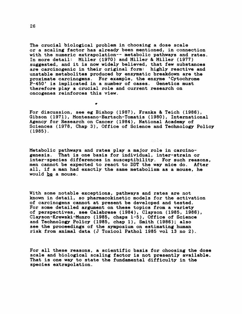
The crucial biological problem in choosing a dose scaleor a scaling factor has already been mentioned, in connectionwith the numeric extrapolation-- metabolic pathways and rates.In more detail: Miller (1970) and Miller & Miller (1977)suggested, and it is now widely believed, that few substancesare carcinogenic in their original form: highly reactive andunstable metabolites produced by enzymatic breakdown are theproximate carcinogens. For example, the enzyme 'CytochromeP-450' is implicated in a number of cases. Genetics musttherefore play a crucial role and current research ononcogenes reinforces this view.

V

For discussion, see eg Bishop (1987), Franks & Teich (1986),Gibson (1971), Montesano-Bartsch-Tomatis (1980), InternationalAgency for Research on Cancer (1984), National Academy ofSciences (1978, Chap 3), Office of Science and Technology Policy(1985).

Metabolic pathways and rates play a major role in carcino-genesis. That is one basis for individual, inter-strain orinter-species differences in susceptibility. For such reasons,men cannot be expected to react to DDT the way mice do. Afterall, if a man had exactly the same metabolism as a mouse, hewould b& a mouse.

With some notable exceptions, pathways and rates are notknown in detail, so pharmacokinetic models for the activationof carcinogens cannot at present be developed and tested.For some detailed argument on these topics from a varietyof perspectives, see Calabrese (1984), Clayson (1985, 1986),Clayson-Krewski-Munro (1985, chaps 1-5), Office of Scienceand Technology Policy (1985, chap 1), Smith (1986); alsosee the proceedings of the symposium on estimating humanrisk from animal data (J Toxicol Pathol 1985 vol 13 no 2).

For all these reasons, a scientific basis for choosing the dosescale and biological scaling factor is not presently available.That is one way to state the fundamental difficulty in thespecies extrapolation.

27

5. The qualitative extrapolation

The main focus so far has been the quantitative extrapolationfrom animal experiments to human populations. This sectionconsiders the qualitative extrapolation-- the idea that if asubstance causes cancer in animal experiments, it is likely tobe a human carcinogen. The idea has intuitive appeal, but theevidence for it is far from solid. The main arguments for thevalidity of the qualitative extrapolation will be reviewed, andthen some evidence from epidemiology will be considered.

The mmaian artument

One oft-recited argument is that humans and mice are bothmammalian species. This verges on sentimentality.. If the testspecies of choice were trout, we would all be vertebratestogether.

The mouse-to-rat argumen

A more substantive argument is that results in the mouse arepredictive for the rat, and so by extension for humans. Thisargument has been made, for example, by Tomatis-Partensky-Montesano (1973).

Table I in Tomatis-Partensky-Montesano (1973) lists the chemicalsconsidered at that time to induce tumors in mice. Were thesechemicals carcinogenic for rats or hamsters? There were 58chemicals, and 11 were classified as negative for the rat, whileanother 7 had not been tested: 6 were negative for the hamster,29 had not been tested. The error rate for rats was 11/51; forhamsters, 6/29.

28

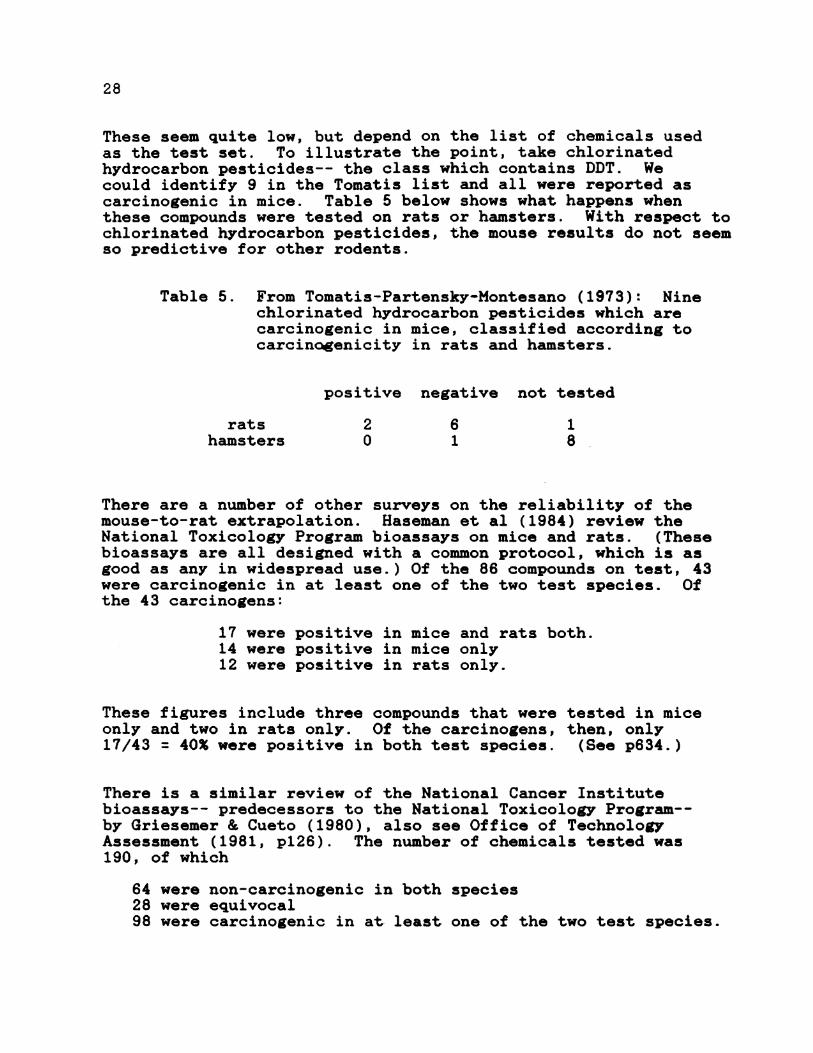
These seem quite low, but depend on the list of chemicals usedas the test set. To illustrate the point, take chlorinatedhydrocarbon pesticides-- the class which contains DDT. Wecould identify 9 in the Tomatis list and all were reported ascarcinogenic in mice. Table 5 below shows what happens whenthese compounds were tested on rats or hamsters. With respect tochlorinated hydrocarbon pesticides, the mouse results do not seemso predictive for other rodents.

Table 5. From Tomatis-Partensky-Montesano (1973): Ninechlorinated hydrocarbon pesticides which arecarcinogenic in mice, classified according tocarcinogenicity in rats and hamsters.

positive negative not tested

rats 2 6 1hamsters 0 1 8

There are a number of other surveys on the reliability of themouse-to-rat extrapolation. Haseman et al (1984) review theNational Toxicology Program bioassays on mice and rats. (Thesebioassays are all designed with a common protocol, which is asgood as any in widespread use.) Of the 86 compounds on test, 43were carcinogenic in at least one of the two test species. Ofthe 43 carcinogens:

17 were positive in mice and rats both.14 were positive in mice only12 were positive in rats only.

These figures include three compounds that were tested in miceonly and two in rats only. Of the carcinogens, then, only17/43 = 40% were positive in both test species. (See p634.)

There is a similar review of the National Cancer Institutebioassays-- predecessors to the National Toxicology Program--by Griesemer & Cueto (1980), also see Office of TechnologyAssessment (1981, p126). The number of chemicals tested was190, of which

64 were non-carcinogenic in both species28 were equivocal98 were carcinogenic in at least one of the two test species.

29

Of the 98 carcinogens:

44 were positive in mice and rats both54 were positive in only one species.

Again, of the carcinogens, only 44/98 = 45% were positive in bothtest species.

Di Carlo (1984) gives a similar picture. Ward-Griesemer-Weisburger (1979) conclude there is a reasonable correlationbetween bioassay results for rats and mice; so does Purchase(1980).

The lack of concordance between rodents and monkeys should alsobe mentioned. For example, 5 out of 6 'model rodent carcinogens'are negative in the monkey: Adamson & Sieber (1983). Results on2-AAF, an intensively studied animal carcinogen, are worth notingtoo. This substance tests as carcinogenic in the cat, chicken,dog, guppy, hamster, mouse, newt, rabbit, and rat: not in thecotton rat, guinea pig, monkey, x/gf mouse, rainbow trout, orsteppe lemming. The tally is 9 to 6. See Weisburger (1981,esp p3); Weisburger (1983, p23) comments on difficulties inmetabolic interpretations. Here as elsewhere, some of the'negative' findings may be due to low power, just as some ofthe positive findings may be artifactual.

There is no clear bottom line to report. Taking all theexperiments at face value, there is some measure of agreementbetween the results for rats and mice, and some measure ofdisagreement. Now rats and mice are much more similar to eachother than either is to humans. The validity of the mouse-to-manextrapolation seems hard to argue on the basis of these data.

Crouch & Wilson (1979) is often cited to show good inter-speciescorrelations of carcinogenic potency. However, Bernstein et al(1985) suggest that Crouch & Wilson may have been misled by astatistical artifact of bioassay design. Zeise-Wilson-Crouch(1984) reports a correlation between toxicity and carcinogenicpotency. If this is real rather than another artifact, it maybe evidence for the cell-killing mechanism of carcinogenesis: seeBernstein et al (1985, p86). Zeise-Wilson-Crouch propose usingthe correlation in quantitative risk assessment, relying on theone-hit model: this ignores much evidence against the model.Crouch-Wilson-Zeise (1987) attempt to refute Bernstein et al(1985), but their statistical argument seems inappropriate.

30

The man-to-mouse argument

Another argument for the qualitative extrapolat'ion is quoted inTomatis (1979):

The difficulties in assessing the significance of experimental[animal] results for predicting similar hazards in humans are bothqualitative and quantitative and can be summariZed in the followingquestions.1. Are chemicals that have been shown to be carcinogenic toexperimental animals also carcinogenic to humans?2. Do experimental animals (rodents, in particular) and humans havesimilar susceptibility to the carcinogenic effect of chemicals, orare rodents incomparably more susceptible than humans?A partial answer to the first question is usually given by reversingthe terms of the question: Most of the chemicals that are carcino-genic to humans are carcinogenic to at least one, and in most casesto more than one, animal species.

The question at issue is this: will most animal carcinogensturn out to be human carcinogens? The argument given is thatmost human carcinogens turn out to be animal carcinogens. Thisblurs together two conditional probabilities: P(A:B) can bequite small, while P(BIA) is quite large. Here, A is the setof animal carcinogens; B, the human carcinogens. So, asTomatis acknowledges, even if most human carcinogens are animalcarcinogens, the converse implication does not really follow.

Nor does the factual base of the argument seem right, as willnow be explained. The test data will be drawn from the IARC,which publishes periodic reviews of the evidence for carcino-genicity of suspect chemicals, compiled by working groups ofexperts.

(The IARC is the International Agency for Research on Cancer,based in Lyon. It is one of the major research agencies inchemical carcinogenesis. Tomatis is a leading experimentalistand at the time of writing, the director of the IARC.)

31

At the time of writing, the most recent review on carcino-genicity was the IARC (1982), with one minor and one majorrevision reported in press: IARC (1987, 1988). Plainly, theclassification of suspect chemicals is a moving target, but thedata base for Tables 6 and 7 below is defined as the IARC (1982).That list of 155 suspect chemicals shows 30 'proven' carcinogensin humans (some well-known carcinogens, like tobacco, had notyet been reviewed by the IARC).

The list also includes information on the animal evidence.The IARC grades the evidence as 'sufficient', 'limited', or'inadequate'. For animals, 'sufficient' evidence means that thechemical causes tumors in two strains or species, or unusuallysevere tumors in one. 'Limited' evidence includes one positiveexperiment. Negative or inconsistent results may be set aside.

The animal data is summarized in Table 6 below and is not in suchgood agreement with the human data after all. As it turns out,there is 'sufficient' proof of carcinogenicity for animals inonly 13/22 = 59% of the human carcinogens.

Table 6. The IARC (1982) list of proven humancarcinogens, classified by degree ofevidence for carcinogenicity in animals.

sufficient 13limited 6inadequate 2no data 1

22animal data

irrelevant 8

32

Consider next the data proposed in Tomatis (1979). His Table 1lists 26 chemicals, groups of chemicals, and processes which are'associated or strongly suspected of being associated with cancerinduction in humans'. (Of these, 18 are considered by the IARCto be proven human carcinogens. For the other 8, the IARC doesnot consider the evidence sufficient, eg, isopropyl oils appearin Tomatis' Table 1, and in the IARC group 3 of things which'cannot be classified as to [their] carcinogenicity in humans.')

V

Of Tomatis' 26 human carcinogens, 17 are carcinogenic in themouse, 15 in the rat, and 6 in the hamster: 65%, 58% and 23%respectively. Thus, there.is a fair amount of discordance amongrodent species, as well as a significant discrepancy between theanimal data and the epidemiology-- which is the next topic.

33

Consistency with epidemiology

How consistent is animal data with epidemiology? This questionseems straightforward, but is full of complexities. There arerelatively few chemicals which have been carefully evaluated byboth methods. Nor does that set constitute a representativesample from the universe of all chemicals. Indeed, the chemicalcarcinogenesis community sets so much store by the man-to-mouseargument that enormous efforts are made to demonstrate thecarcinogenicity in mica of likely human carcinogens; see Wald& Doll (1985, p4).

As before, data from the IARC (1982) will be used. Their Table 1reports on 155 chemicals, groups of chemicals (eg, soots, tarsand oils) and processes (eg, hardwood furniture manufacture)tested for carcinogenicity. With respect to 19-- including eghardwood furniture manufacture, 'certain combined chemotherapyfor lymphoma', and various forms of oral contraceptives-- theIARC judges that animal experiments are irrelevant. In somecases, they are clearly right and in others they may be wrong,but for present purposes we accept their judgment. In 3 casesthere are no animal data. Eliminating the 19 irrelevant casesand the 3 without data leaves a test set of 133 chemicals andgroups of chemicals.

The IARC considers three types of evidence: epidemiologicalstudies, animal bioassays, and short-term tests (for muta-genicity in vitro). The grades of evidence were discussedabove: for humans, 'sufficient' evidence means goodepidemiology.

34

Table 7 below classifies the test set by grade of evidencefor carcinogenicity in humans and animals (as determined bythe IARC). There is a fair amount of discord in Table 7: withrespect to only 21% of the animal carcinogens is there 'suffi-cient' evidence for human carcinogenicity.

The 'insufficient' category in the table combines IARC grades oflimited or inadequate evidence. This may be unconventional, butseems fair, given the IARC definitions. Indeed, for reasons tobe given in the next section, even 'sufficient' animal evidencemay not be compelling. ,

Table 7. The test set of 133 relevant chemicals andgroups of chemicals reviewed by the IARC,for which data is available, classified bygrade of evidence for carcinogenicity inanimals and humans.

in human

sufficient

insufficient

grade of evidence forcarcinoxenicitv in animals

suffic'lent 0nufficient

21% 11%

79% 89%

100% 100%

number 61 72

35

In principle, the evidence in Table 7 is decisive: carcino-genicity in lab animals is poor evidence for an effect in humans.Questions about the representativeness of the test set and doubtsabout the quality of the underlying studies (both positive andnegative) weaken this conclusion appreciably. We do not take upsuch questions because we made no systematic review of the under-lying studies, and only report the classifications reported bythe IARC.

The overall conclusion from Table 7: the research reports ofthe cancer community (even taken at face value) do not sustainthe conventional arguments for the validity of the qualitativeextrapolation. For a more detailed discussion of inconsistenciesbetween animal evidence and epidemiology, see Wald & Doll (1985).For an establishment view of the evidence, see Wilbourn et al(1986); the correlation in their Table III reflects onlycompounds which are positive in humans.

We remain sympathetic to the idea that animal data have somepredictive value for carcinogenicity in humans, at least quali-tatively; and perhaps even to establish rankings of potentialhazards as suggested by Doll & Peto (1981, ppl21Sff). Butthe evidence for such propositions is surprisingly weak.

Experimental studies to quantify inter-species differences insensitivity would clearly be very useful, if expensive. Researchto determine the biological bases for these differences would beeven more useful.

36

6. Review of carcinogenesis experiments

Some general questions will be raised about the qualityof animal experiments on carcinogenicity, and then the DDTliterature will be reviewed, to illustrate the points. Thereturn out to be substantial inconsistencies in the experimentaldata, perhaps attributable to the multiplicity of endpoints anduncontrolled variation. Proposals are made for improving theexperiments.

Reproducibility of results seems to be a crucial issue, anda preliminary remark on definitions is in order. As noted above,cancer is not a unitary,disease. In animal experiments, thereare some 25 major organ systems which are checked by autopsy fortumors of various types. Even the type of lesion which willbe taken as evidence for carc'inogenicity may only be decidedduring the course of the experiment.

There are marked differences in carcinogenicity across sexes,strains and species. Often, the same chemical will cause onekind of cancer in one experiment, and another kind in anotherexperiment (but see Gold et al 1986b). Indeed, the most hard-bitten advocates of animal experiments do not claim to be ableto predict which organ will be affected in humans by a chemicalwhich is carcinogenic in animals (see eg Wilbourn et al 1986,esp Table II).

Some of the differences in carcinogenic response must bedue to differences in the biology, and some to uncontrolledvariation in the experimental design. What are the likelysources of such variation? For one, animals may not be properlyrandomized to the various treatment groups; and there may bestrong litter effects, especially in multi-generation studies(Grice-Munro-Krewski 1981, Turusov et al 1973). Likewise,animals are seldom randomized to cages; but position in the rackseems to be a risk factor for cancer (Lagakos & Mosteller 1981).

Indeed, many other apparently extraneous factors substantiallychange the incidence of tumors. These include stress, calorierestriction, and viral infection. See eg Clayson (1975,1978),Gellatly (1975), Jose (1979), Peto (1980), Roe (1981), Tannenbaum(1940-2), National Academy of Sciences (1983b).

A final example of a design problem: the pathologists whoidentify the tumors often know the treatment status of theanimals, and this leaves room for bias in the diagnostics.Pathologists see themselves as professionals exempt from bias andresist suggestions for blinding, as in Weinberger (1973, 1979):despite the author's intentions, these papers vividly show howknowledge of dose status can influence diagnostic results.

37

The magnitude of this bias is not easy to document fromthe medical literature. For some evidence in the setting ofclinical oncology, see McFarlane-Feinstein-Wells (1986); forevidence on bias in reading echocardiograms, see Tape & Panzer(1986); on X-rays, see Reger-Butcher-Morgan (1973) or Reger-Petersen-Morgan (1974). For evidence on the variability inreading pathology slides, see eg Siegler (1956) or Metter etal (1985); and for a recent review, Swan & Petitti (1982).

The high spontaneous tumor rates in the experiments contributeto the difficulty: MuItiple endpoints matter, because there aremany types of tumors and many sites. Then artifacts of chanceor poor design create the likelihood that in one experimentthere will be a high cancer rate at one site, and in anotherexperiment, the excess will be observed at another site, evenif there is no real carcinogenic effect.

For a general discussion of excess variation, see Haseman (1983)who reviews 25 National Toxicology Program bioassays on variouschemicals and shows that increases in cancer at one site arematched by decreases at another site. Such decreases are usuallyexplained away by asserting that the animals in the treatmentgroups do not live long enough to develop tumors. Hasemanrejects this explanation because the animals in the treatmentgroups live a bit longer than the controls: the difference issmall, but statistically significant. (In all cases, the testspecies was the Fischer 344 rat; the increased tumor rates weremainly in the liver; the decreases, lymphomas and leukemias.)

These points will be illustrated using long-term animalexperiments where DDT, DDD and DDE was fed to mice, rats orhamsters. To minimize selection bias, we took only papersreferenced in IARC (1974, 1979, 1982). This screened out somebad studies, and some good ones. Too, we may have missed a fewpapers referenced in IARC (1974) but not summarized there.The sample is listed in Table 8 below, with comments.

38

Table 8. The sample of papers.

The mouse (11 papers, 9 studies).

Innes et al (1969). JNCI 42 1101.Two strains of mice, X = (C37BL/6 x C3H/Anf)F1 and Y = (C37BL/6x AKR)Fl. Tested 120 compounds, with about 20,000 mice; found Itcarcinogenic, including DDT at 140 ppm; found DDD and 19 othercompounds 'require further evaluation', but did not report data.Common control group. Survival is to term, and the denominator forcancer incidence is the number sent to necropsy.

Kashyap et al (1977). Int J Cancer 19 725.Pure Swiss inbred mice. Reports multiple experiments; we analyzeonly the feeding experiment on DDT at 0 or 100 ppm. Survival is to80 weeks.

Shabad et al (1973). Int J Cancer 11 688.Multi-generation study on A-strain mice. The design is not easy todiscern from the paper: compare IARC (1974, p98). Table 11 reportson DDT at 0 or 10 ppm, pools sex and generation, and gives six-monthsurvival. The tumors are lung adenomas, and according to theauthors, 'No other tumors were observed in the treated animals'.

Tarjan & Kemeny (1969). Fd Cosmet Toxicol 7 215.Multi-generation study on BALB/c mice, DDT at 0 or 3 ppm.Denominators shown in Table 3 for males and females combined; weelected to pool Ft-5.

Terracini et al (1973a). Int J Cancer 1t 747.Terracini et al (1973b). In WB Deichmann, ed. Proceedings ofthe 8th Inter-American Conference on Toxicology: Pesticides andthe Environment, A Continuing Controversy.Multi-generation study on BALB/c mice; DDT at 0, 2, 20, 250 ppm.Survival among the males was poor, in part due to fighting; soresults are given only for females. Results in the second paper werenot in usable format for present purposes. Data are from Table IIIin the first paper; denominators are initial number of mice; livercysts not counted.

Thorpe & Walker (1973). Fd Cosmet Toxicol 11 433.CFI mice. We analyze only the DDT results, at 0 or 100 ppm.Data from Table 2. Liver tumors (a+b) taken relative to effectivenumber; at other sites, relative to initial number of animals.Survival at 21 months (Table 1).

Tomatis et al (1972). Int J Cancer 10 489.Turusov et al (1973). JNCI 51 983.Multi-generation study on CFI mice. DDT at 0,2,10,50,250 ppm.Hemangioendotheliomas not counted.Data in the second paper not in usable format.

39

Table 8. The sample of papers, continued.The mouse, continued

Tomatis et al (1974). JNCI 52 883.CFI mice. Common control group. Three treatment groups:i) 250 ppm DDD ii) 250 ppm DDE iii) 125 ppm DDD + 125 ppe DDE.

Walker et al (1973). Fd Cosmet Toxicol 11 415.CF1 mice. Reports multiple experiments. We analyze only the DDTresults, at 0, 509 100 ppm. Data from Table 4. Liver tumors of typea & b are pooled, as are adenomas and carcinomas of the lung.Incidence rates are relative to the initial number of animals.

The rat (9 papers)

Cabral et al (1982). Tufori 68 It.MRC Porton rats; DDT at 0,125,250,500 ppm. 80 week survival.Incidence rates relative to initial numbers.

Deichmann et al (1967). Toxicol Appl Pharmacol 11 88.Osborne-Mendel rats; synergy experiment; we analyse only data on DDT,at 0 or 200 ppm. Survival at 24 months. Incidence rates relative toinitial numbers.

Fitzhugh & Nelson (1947). J Pharmacol & Exp Ther 89 18.Insufficient data for tabulation.

Lacassagne & Hurst (1965). Bull Cancer 52 89. No control group.

Nishizumi (1979). Gann 70 835.Synergy experiment, reports only on DDT in conjunction with other carcinogens.

Radomski et al (1965). Toxicol Appl Pharmacol 7 652.Osborne-Mendel rats; synergy experiment; we analyze only data on DDT,at 0 or 80 ppm. Incidence rates relative to initial numbers;benign and malignant tumors pooled.

Rossi et al ( 1977). Int J Cancer 19 179.Wistar rats; DDT at 0 or 500 ppm; survival at 100 weeks.

Treon & Cleveland (1955). J Agric Fd Chem 3 402. No data.

Weisburger & Weisburger (1968). Fd Cosmet Toxicol 6 235. No data.

The hamster (2 papers)

Agthe et al (1970). Proc Soc Exp Med NY 134 113.Reports only a small number of tumors, and not by site.

Cabral et al (1982). Tumori 68 5.Syrian golden hamster; DDT at 0,125,250,500 ppm; survival at 50 weeks.

40

Most of the authors did address the issue of comparability inhusbandry among the various test groups, but not in convincingdetail. No paper discussed the issues created by multipleendpoints, or 'open' reading of slides. By contrast, much spaceis routinely spent describing comparative pathology of tumors,with illustrations-- clearly the topic of interest.

No experiment in Table 8 had two test species, although onedid have two strains of mice. Only two of the papers summarizedin Table 8, both from the same laboratory, explicitly mentionrandomization of animals to treatment. Since there are a varietyof standard randomization schemes, we lean to the view that theother authors did not, in fact, randomize the animals to thevarious dose groups. (We can also report that in one majorinstitution, 'randomization" means that a technician takesanimals by hand out of a cage.)

Table 9 below attempts to analyze the sample of papers in aunified way. It is based on the chi-squared test for trend,as in Armitage (1955). In effect, the test regresses the site-specific incidence of cancer on the dose, weighting by thenumber of animals at risk, and divides the slope by its standarderror, which is estimated on the hypothesis of binomial vari-ation. If there are only two dose groups, the test coincideswith the usual one for equality of two binomial probabilities.

Epidemiologists routinely use this procedure to see whether aresponse goes up with dose, or down, or sideways. Simplicityis its virtue, but it does not distinguish between linear orcurvilinear responses. On the other hand, with only a limitednumber of dose groups, such distinctions may not be feasible.

The table reports the ratio Z of the estimated slope to itsstandard error. If Z is positive, the rate tends to go up withthe dose, and DDT is harmful; if negative, the rate goes down,and DDT is protective. If Z is bigger in absolute value than 2,the effect is 'statistically significant'.

(In many cases, the sample size is so small that the asymptoticsare only a rough guide to the significance level; Fisher's exacttest was feasible, but seemed unnecessarily complicated for ourpurposes, which are largely descriptive; likewise for maximumlikelihood estimates of potency.)

Table 9. A study of studies: the impact of DDT andits metabolites on mice, rats and hamsters.Z-tests for dose-response in death rates andtumor incidence rates by site.

Deaths Liver LungsLymphoaa Oste- Kid- Testes Hame-Leukemia ama neys Ovaries aries

Pitui- Adre-tary nals

MICE

Innesx N -1.4 5 .7 '-1.1X F 4 4 -.8y .4 4 0.0Y F 1.1 1.2 -.8

Kashyap-.5 1.4

F 0.0 1.7Shabad -.7 0.0Tarian ? ?

.21.34

1.2 2.01.0 2.05 0.0

? 6

7~~~~~~~~? ?7

? 7?

7 ? ? 7? 7

? 7 7 7

0.0 0.0 0.0 0.0 0.0 0.0 0.0

7 7 7 7

Terracini 73aP F

Fl FThorpe

F

Tomatis 72P "P F

Ft N

Ft F

Tomatis 74DDE N

FODD N

FNix N

F

-,9 9 -1.61.5 14 .9

-2.8-4

.8 5 -1.9 -2.12.0 6 -2.6 -1.5

31.94

2.0

7

8

-1.3.2.7

1.7

5 -2.010 2.16 -.210 -2.1

5

122.3.3

510

-2.1-34

4

-.3-3

Wal kerN L.7 4 1.0F -.2 5 -2.0

-2.2-1.2-1.4

-.7

-4

-5-.7.6

-3-.4

-. I-.a

-1.6.7

.6

-2.3-.3

-1. I-.8

-.6

7 7 7 7 77 7717 7 ?v77 7

-.6-.6

-1.3_.5

-1.0

0.0

-.8 ? ? ? ?.9 ? ? ? ?

7

-1.2

-t.7

0.0 ? ? ?-.6 ? ? ?0.0 ? ? ?-.6 ? ? ?

? 7 7 7 7 7

?? 7 7 ? 7

79 ? ?7 7

7 7 7 7 7 7

7) 7 7 )

-.01 ? .05 2.0 ? ? ? ?-2.0 ? -1.3 -1.2 ? ? ? ?

41

Study

Thy-roid

Table 9. Continued. A study of studies: the impact of DDTand its metabolites on mice, rats and hamsters.Z-tests for dose-response in death rates andtumor incidence rates by site.

Deaths Liver LungsLymphosa Oste- Kid- Testes Name-Leukesia ama neys Ovaries aries

Pitui- Adre Thy-taries nals roid

RATS

Cabral

Dei chmannNF

Radomski

Rossi

M 1.2 .9 ?F .9 2.8 ?

-.8-2.7

0.0 0.00.0 0.0

U?7 ? ? -.9 1.4 1.1?7 ?7 ? 1.4 -2.9 -1.2

0.0 ? ?-1.0 ? ?

? -1.0? -1.7

N ? 0.0 1.0 0.0 ? ? 0.0 0.0F ? 0.0 1.7 0.0 ? ? 0.0 -1.0

N 1.1 4 -.9F .3 5 .7

.1 ? ?

.1 ? ?

0.0 1.01.0 -1.0

-1.6 .2 ? -2.3.1 -.6 ? -1.4

HAMSTERS

N -.4 .3 ?F -.5 0.0 ?

? ? ? ? ? d0.07 ? ? ? ? .2

1.6 1.42.2 .6

SUMMARY

Z-values

7 21 512 6 7

0.0 exactly 1 6 3

1O 0 71 0 7

4 0 0 1 0 0 1 05 2 1 3 2 3 2 5

4 1 2 3 4 3 1 2

9 7 6 6 6 1 2 08 1 0 0 1 0 1 0

4 23 25 21 21 27 27 27

42

Study

? 1.9? 0.0

Cabral

.31.1

+2.0 ar more+0.1 to +1.9

-0.1 to -1.9-2.0 or less

? 1) 1)

? 1) 7

... 3 1 5

43

Authors were not uniform in reporting survival data; often atable was provided, sometimes only a graph-- which we did ourbest to read. Where possible, 90-week survival was tested inTable 9; sometimes, another period had to be substituted.

There is a preference in the field for reporting tumor incidenceby site and sex, so we followed suit. Authors were not at alluniform in choice of sites to report; a question mark in thetable means no report for that site. Since authors will reporton the sites with many tumors, a question mark suggests the lackof any carcinogenic response.

U

Some authors failed to report the sexes separately, and thenresults are given for all animals pooled. With one exception,we reported as separate experiments the separate generations inmulti-generation studies: P is the parental generation, Fl thefirst generation of offsprings, etc.

Many authors-- but by no means all-- report the 'effectivenumber', ie, the number of animals alive in each group at thetime of the appearance of the first tumor in that group. Thisrepresents a partial adjustment for differential mortality inthe test groups, especially due to the toxicity of the testsubstance. If the effective number is given, incidence ratesare computed relative to it. Otherwise, the denominator is takeneg as the number of animals sent to necropsy, or the number ofanimals initially assigned to the group. (See Table 8 above fordetails.)

Tallies are shown at the bottom of Table 9, and are collectedin Table 10 for all sites other than the liver, and all experi-ments. (In the last line of Table 10, there are 180 combinationsof sites and sub-experiments where no tumor incidence rates werereported.)

44

Table 10. Z-statistics for dose-response intumor incidence rates by site, otherthan the liver. Mice, rats, hamsters;DDT and metabolites.

+2.0 or more 11+0.1 to +1.9 30

0.0 exactly 23

-0.31 to -1.9 44-2.0 or less 18

no data 180

The binomial model behind the Z-test represents some idealizationof the experimental results. It assumes randomization of animalsto treatment and conditions of husbandry, and no observer bias.Of course, even if the chemical has no effect, the actualvariation may be appreciably larger than binomial, forreasons indicated above.

Insofar as the binomial model has any validity, with respect tomice the data suggest that DDT shortens the lifespan and causesliver tumors. At other sites, and for other species, the picturecan only be described as mixed. Indeed, taking the results ofthe bioassays at face value, DDT seems on balance to inhibittumor development. (But see Rossi et al 1983 on DDE andhamsters; also Cabral 1985 on DDE and rats.) Other evidence onprotective effects has already been presented (Haseman 1983);and for DDT itself, Okey (1972).

45

With respect to evidence for the carcinogenicity of DDT, muchrides on the interpretation of liver tumors in mice. And forworkers in the field, this is something of a controversial area.As the Office of Science and Technology Policy (1985) says:

Critical to decisions about carcinogens is the biologicalsignificance and human relevance of certain types of tumors,particularly the liver tumors in the mouse. This matter has beenthe subject of heated debate for the past 15 years*....

U

The discordance of the results in Table 9 is its message. Ofcourse, even with a good protocol, maintaining quality controlis difficult, and the difficulty increases with the number ofanimals; this may put an upper limit on the power of a biossay.For other discussions of these issues, see Gart et al (1985),IARC (1980), the National Toxicology Program (1984), the UKDepartment of Health and Social Security (1982).

None of the NTP or NCI bioassays turned up in the test set;the protocol for those bioassays seems much better than thestandard in Table 8, especially with respect to multipleendpoints. However, for a review of the NCI bioassays alongpresent lines, see Salsburg (1983). For a useful summary ofa large set of bioassay results in standard format, see Goldet al (1984).

46

Much more care is needed in defining endpoints before theexperiment starts. We also recommend using statistical analyseswhich recognize the multiple-endpoint problem explicitly. It maybe helpful to pool results across sites and even sexes, testingwhether the percentage of tumor-bearing animals in the differenttreatment groups is dose-related. In this regime, correction forother causes of mortality would be quite important.

Pooling is contrary to standard practice in the field, whichcalls for separate analysis by site and sex. See Haseman etal (1986), who review the impact of pooling on NTP test results;of course, a difference in results does not show that one ruleor another is superior. The authors argue that stratificationshould increase statistical power; and that combining tumors ofdifferent types will not lead to biologically meaningful results.

Their first set of arguments may be dominated by the multipleendpoint problem, which compromises all bioassay results whetherapparently significant or apparently insignificant. On the otherhand, as they point out, background tumor rates are so high inrats (97% for males, 83% for females) that increases would bevery hard to detect. The possibility of analysis by major tumortypes might be worth exploring; equally, the Value of testing ona strain with such a high spontaneous tumor rate would be worthreconsidering-- even for strong proponents of bioassays.

Haseman et al's biology argument provides an effective critiqueof extrapolations from the most sensitive site in test animals toall tumors in humans. That sort of worst-case analysis is commonpractice in risk assessment: indeed, as noted above, animalexperiments do not predict the sites that will be affected inhumans (Wilbourn et al 1986). If it makes no sense to poolresults for the animals, it makes no sense to pool predictionsfor the humans. Also see US Environmental Protection Agency(1986).

Multiple-comparison techniques might be a useful supplementto pooled analyses, as heuristic aids in identifying the sitesresponsible for a dose-response relationship. (The NCI/NTPbioassay protocol already uses such methods.) Anomalies such asthe appearance of rare tumors would also have suggestive value.However, given the complexities of real bioassays, statisticalanalysis cannot by itself screen out the artifacts. Replicationis crucial.

To summarize our other recommendations: the necropsy work shouldbe done 'blind' so far as possible. Strict attention should bepaid to randomization, using computer-generated random numbers orthe like to make assignments to the different cages and treatmentgroups.

This completes the discussion of the animal experiments; thenext topic is the usual justifications for risk assessment.

47

7. What do others say?

There is a large scientific bureaucracy, in Washington andelsewhere, concerned with the regulation of chemicals onthe basis of animal studies. What do they say in defenseof the activity? The most interesting documents seem to beEnvironmental Protection Agency (1975), Food Safety Council(1980), IARC (1979, 1980, 1982, 1983), National Academy ofSciences (1975, 1978, 1980), Office of Science and TechnologyPolicy (1985), Office of Technology Assessment (1977, 1981).

The Food Safety Council'

The Food Safety Council (now defunct) was jointly funded byindustry, consumer groups, and government, to review doseresponse modeling in the setting of safety standards. TheScientific Committee included Jerome Cornfield and John vanRyzin. Earlier, we reviewed some of the discussion in thereport (Food Safety Council 1980). From pp711, 718, 730.

Human risk assessment is a very inexact exercise, based largely upontheoretical assumptions concerning interspecies extrapolations. Theuncertainties involved should be fully recognized by the scientificcommunity and society.

Regulatory decisions, hoiwever, must be made even in the absenceof complete knowledge. Decisions based on informed scientificJudament, moreover, may be more easily criticized than thosebased on the systematic application of an objective set ofdecision making criteria which provide insofar as possible forthe biological and statistical uncertainties involved.[emphasis in original]

..the low-dose extrapolated risk estimates are highly modeldependent. Because of this inexactness (sic] of the behavior of themodels in the low-dose range, plus the fact that they cannot befirmly justified on either statistical (goodness-of-fit, say) orbiological grounds, the choice of how one does the extrapolation isprimarily a matter of judgment.

In cruder terms, the argument comes down to this: the regulatoryprocess must proceed, whether or not there is a suitable scien-tific basis for it. And it is better to avoid the appearance ofsubjectivity by deriving the risk estimates from a model, eventhough choosing the model is itself a critical step in theprocess, and a highly subjective one-- but not so visible.

48

The IA

The IARC research program is well respected, and draws workinggroups of scientists from all over the world. However, canceris more than a scientific puzzle, and the workling groups seem towalk a fine line. The IARC (1982, p13) was fairly blunt aboutrisk assessment:

At present, no objective criteria exist to interpret data fromstudies in experimental animals or from short-term tests directly interms of human risk.

Here they are, a year later (IARC, 1983, p18):

In the absence of adeqcuate data in humans it is reasonable,, forpractical purooses. to regard chemicals for which there is sufficientevidence of carcinogenicity in animals as if they presented acarcinogenic risk for humans. The use of the expressions 'forpractical purposes' and 'as if they presented a carcinogenic risk'indicates that at the present time a correlation between carci-nogenicity in animals and possible human risk cannot be made on apurely scientific basis, but only pragmatically. Such a pragmaticalcorrelation may be useful to regulatory agencies in making decisionsrelated to the primary prevention of cancer. [emphasis in original.3

In the present state of knowledge, it would be difficult todefine a predictable relationship between the dose (mg/kg bw/day) ofa particular chemical required to produce cancer in test animals andthe dose which produce a similar incidence of cancer in humans. Somedata, however, suggest that such a relationship may exist tRall,197, National Academy of Sciences 19753, at least for certain classesof carcinogenic chemicals, but no acceptable methods are currentlyavailable for quantifying the possible errors that may be involved insuch an extrapolation procedure.

The first paragraph still makes our point, if diplomatically.The second paragraph only says that while it may be possible toextrapolate from the mouse to man, at present it is impossibleto estimate the resulting errors.

49

In the passage quoted above, as in many other such officialdocuments, the NAS (National Academy of Sciences, 1975) iscited to support extrapolations from animal data. This NASstudy is based on a review of risk assessments for six chemicals.The observed differences ranged up to a factor of 500. Thatstill understates the problem, since the human risk 'data' arethemselves obtained by modeling, which appears to force someagreement on the estimates. For other studies by the NAS,see below. Rall (1977), also cited by the IARC, is notpersuasive either. Indeed, Rall presents only two systematicsurveys: one is the NAS (1975), and the other is about toxicitynot carcinogenic'ity.

The OSTP

The Office of Science and Technology Policy (OSTP) is thePresident's advisory group. They reviewed cancer risk assessmenttechnologies in 1985 (also see US Interagency Staff Group onCarcinogens 1986). Here is what they have to say:

Many components of the risk assessment process lack definitivescientific basis....

Many scientists would agree that, while there is a significant amountof evidence to support qualitative animal to human extrapolation forcarcinogenesis, the evidence falls short of establishing thisproposition as a scientific fact (when determining the response ofdifferent species to chemicals, many chemicals appear to becarcinogenic in one species or strain and not in another, even whenonly rodents are being compared). Nonetheless, this principle hasbeen accepted by all health and regulatory agencies and is regardedwidely by scientists in industry and academia as a justifiable andnecessary inf erence.

At first reading, the OSTP seems to be contradicting itself.However, 'justifiable and necessary' only means that they can'tdo risk assessment otherwise.

50

The OTA

The Office of Technology Assessment (OTA) is the advisory groupfor Congress. They have reviewed the cancer risk assessmenttechnology at least twice: in 1977 when the saccharin contro-versy was raging, and again in 1981. In 1977, they were quiteoptimistic about the technology; even so, here they are on p82:

It is generally accepted that an animal carcinogen is also a humancarcinogen. Extrapolation between cancer incidence in animalsand expected incidence in humans is necessary to quantify therisk for human population; from exposure to a chemical.

'Necessary' is to be distinguished from 'scientificallydefensible'.

By 1981, the OTA was much more critical of the technology--although still for it. From the OTA (1981, pp12-13, 113, 122):

Opinions differ about whether and how extrapolation methods should beused in estimating the amount of human cancer that might be caused byexposure to a carcinogen.... The disagreements among the groups whohold different opinions about use of extrapolation methods are vocaland current.

The fact that some regulations are based on nonhuman test systemsshows that proof that a chemical is a human carcinogen is notdemanded. This illustrates that prevention of cancer is seen as soimportant that it is appropriate to make decisions to restrictexposures before human damage is observed.

A substantial body of experimentally derived knowledge and thepreponderance of expert opinion support the conclusion that testingof chemicals in laboratory animals provides reliable informationabout carcinogenicity.

With respect to the last paragraph, the 'preponderance ofexpert opinion' is hard to assess. But the 'substantial body ofexperimentally derived knowledge' seems quite ambiguous on thecrucial question of extrapolating risk estimates from laboratoryanimals to people.

51

The EPA

The Environmental Protection Agency (EPA) is one of the leadagencies in regulating carcinogenic hazards. In 1972, theybanned DDT; and in 1975, they wrote a white paper justifying thedecision. From pp87 and 252:

Although the target tissue may be different, the souse can, inspecific cases, serve as a reliable and proven indicator of thecarcinogenicity of a cheilcal in other species including man.However, although carcinogenic effects in mice are valid when dealingwith certain chemicals, the results can vary greatly depending on thecompound tested and may not always be a reliable basis forextrapolation to other species.

Proponents argue that DDT has a good human health record and thatalternatives to DDT are more hazardous to the user and more costly.Opponents to DDT, admitting that there may be little evidence ofdirect harm to man, emphasize other hazards connected with its use.

In sum, the mouse is a 'reliable and proven indicator' ofcarcinogenicity, which works for some compounds but not others,perhaps not even for DDT.

52

The Saffiotti- reloort

An ad hoc committee of fairly determined bioassay proponentsexpressed its views in a 1970 report to the Surgeon General.The chairman was Umberto Saffiotti, then Associate ScientificDirector for Carcinogenesis at the National Cancer Institute.(This passage is quoted in Epstein 1979.)

Evidence of negative results, under the conditions of the test used,should be considered superseded by positive findings in other tests.Evidence of positive results should remain definitive, unless anduntil new evidence conclu,pively proves that the prior results werenot causally related to the exposure.

In order to evaluate the hazard of a chemical for man, one mustextrapolate from the animal evidence. It is essential to recognizethat no level of exposure to a carcinogenic substance, however lowit may be, can be established to be a 'safe level' for man.

In recognizing a chemical as a carcinogen, the limiting factor is thesensitivity and specificity of the bioassay system used. A bioassaysystem designed to detect tumor induction only at or above a givenlevel under the conditions of the test (eg, a 25 percent incidence ofa specific tumor type) will fail to reveal carcinogenicity belowthat level. Compounds whose carcinogenic effects fall belowspecific bioassay detection limits must not be consideredinnocuous.

Chemicals should be subjected to scientific scrutiny rather thangiven individual 'rights'; they must be considered potentially guiltyunless and until proven innocent.

The view seems to be that chemicals are carcinogenic untilproven otherwise, and proof of innocence is almost impossible.The dictum that positive evidence supersedes negative is hardto justify, given the degree of inconsistency within the animalexperiments, or the conflict between animal data andepidemiology.

53

The NAS

The National Academy of Sciences (NAS) conducts studies forgovernment agencies, using ad hoc panels. They reviewedcancer testing technology in 1975, 1978, 1980, and 1983. The1975 report was fairly positive; the 1978 and 1983 reports, quiteguarded. The 1980 report (especially chap 4 and appendix A) wasextremely critical; eg, from pp81-83:

V

.... current understanding of carcinogenesis and related pathologiesis not adequate to permit reliable extrapolations from animalexperimentation and simpler assay systems to actual quantifiedhazards to human health.... at least two extrapolations ofinadequately tested reliability must generally be applied to bioassaydata to derive estimates of human cancer incidence.... inferencesdrawn by means of current extrapolation methods lack scientificjustification....the provision of a sophisticated quantitativeestimate of human cancers provides a high potential formisinterpretation because the estimates may be used without therequired attention to the inherent constraints....users are so hungryfor numbers that quantitative estimates, once presented, take on alife and authority of their own, despite all the reservations that[the analyst] may attach to them....

54

Other authors

Ames

Ames (1983) gives a reductio-ad-absurdum argument againstquantitative risk assessment. In brief, every day peopleingest 'natural' carcinogens and mutagens: eg, M-IQ in broiledhamburger, aflatoxins in peanut butter, phorbol esters in herbteas, theobromine in cocoa, safrole and piperine in sassafrasor black pepper, hydrazines in mushrooms, furocoumarins incelery.

The methodology of quar itative risk assessment-- extrapolationfrom bioassays and short-term tests-- shows that the risks fromthe natural carcinogens dominate the risks from environmentalcontamination by chemicals. (Cigarette smoking, some drugs, andsome occupational exposures do present extraordinary hazards.)Also see Ames-Magaw-Gold (1987), Felton & Hatch (1986),Knudsen (1986), and the symposium report in the August, 1986issue of Environmental Health Perspectives.

Doll & Peto (1981. PP1215-16)

.... animal feeding studies have great value in certain circumstancesbut may not offer an uncomplicated and straightforward means ofdiscovering preventable causes for the majority of human cancers, andat the very least it certainly does not seem likely that they canoffer a reliable means of estimating quantitative human hazards.

If our perspective on both short-term and animal tests is accepted,then quantitative human 'risk assessment', as currently practiced, isso unreliable, suffering not only from random but also probably fromlarge systematic errors of unknown direction and magnitude, that itshould definitely be given another name: 'Priority setting' mightperhaps be a more honest, although less saleable, name.

55

Tomatis (1977. Dv1349 & 1352)

We all agree that the mouse should be discarded as a testing tool ifa better experimental model can be found. At present, however, itseems that it is no worse qualified than any other species fordetecting the carcinogenicity of environmental chemicals and forpredicting a possible human hazard.

It is clear that, at present, there is no general consensus on thevalidity of using experimental results to predict human hazards.

Tomatia-Breslow-Bartsch (1980)

The good empiric correlation between human and experimental animaldata for the limited number of chemicals for which both human andexperimental data are available indicates, as shown previously, thatexperimental animal data may predict a qualitatively similarresponse in humans, although the validity of this empiriccorrelation cannot be extended to predict possible quantitativevariations of that response in different species. The data obtainedin animal tests may, however, represent different degrees of evidenceof a carcinogenic effect, this drawback being due mainly to ourinsufficient knowledge of the mechanisms of carcinogenesis.

The fact that the appropriateness of the various models is a matterof considerable debate within the scientific community, and that fewrelevant data are available to the proponents of either side, servesto emphasize the uncertainties inherent in the process ofextrapolation.

56

8. Conclusions

Bioasaays

The IARC (1980) guidelines on the conduct of bioassays seem quitesound, and we wish they were more often followed in practice.Since bioassays are inherently statistical, randomization iscritical-- to treatment groups and to conditions of husbandry.'Blinding' the necropsy work would also be a valuable precaution.

The multiple endpoint problem is quite serious. A possiblesolution would be to pool results across sites and even sexes,and test whether the percentage of tumor-bearing animals in thedifferent treatment groups is dose-related. In this regime,correction for other causes of mortality would be quiteimportant.

If the idea of pooling is accepted, multiple-comparisontechniques might be a useful supplement, at least as heuristicaids in identifying the sites responsible for a dose-responserelationship. Anomalies such as the appearance of rare tumorswould also have suggestive value. However, given the complexi-ties of real bioassays, statistical analysis cannot by itselfscreen out the artifacts. Replication is crucial.

Qualitative extrapolation

If a substance is carcinogenic in a bioassay, we think that issome evidence for carcinogenic potential in humans. If thebioassay was well run, the evidence is stronger. Replicabilityacross experiments and across species makes the case evenstronger. Conversely, flaws in the experiment or failure toreplicate weaken the argument. As Wald & Doll (1985, p225) say:

Only one rule is absolute: that all the available evidence mustalways be taken into account.

The validity of the qualitative extrapolation seems to be a topicon which much useful research could be done. A feasible-- butexpensive-- program would call for a series of good bioassays ona representative sample of agents and species, with the object ofmeasuring inter-species differences in sensitivity. Furtherresearch into the biological parameters which determine speciessusceptibility would be even more useful.

57

Quantitative extrapolation

In the present state of the art, making quantitative assessmentsof human risk from animal experiments has little scientificmerit. Valid extrapolations would be possible only on the basisof mathematical models grounded in biological reality, andcarefully tested against empirical data.

As presently formulated, public policy depends on quantitativerisk assessment. This guarantees a steady supply of suchassessments; and an equally steady supply of apologetics writtenby scientific oversight committees who ask, "What bettertechnology is there?" A wiser course might be to reformulatethe policies so that regulation could be accomplished on thebasis of what regulators actually knew, rather than what theywished they knew.

58

Policy im-Plications

We find that the models now used in risk assessment do not havemuch by way of scientific foundation, yet we do not propose newmodels. This position cannot be agreeable to workers in thefield, or to anyone wanting statistics used in settlingpublic-policy questions. On the other hand, a disagreeableposition may be right.

We sympathize with the goal of bringing some statistical orderinto cancer prevention, and regulating chemicals on the basis ofextrapolation from animal experiments. We also like the ideaof advancing biological knowledge through statistical models.Our concern is the feaibility of such enterprises, given thepresent limits to knowledge in biology and statistics.

At one time, the multi-stage model seemed like a promisingavenue to explore, and it has lead to some good research. Butin the end, the scientific claims made for that model (and forothers like it) must be judged by ordinary scientific standards.If we are right about the technical issues, quantitative riskassessment cannot be justified on those standards. It may beadvisable to give up the pretense of a scientific foundationwhere none exists.

An objective procedure for licensing chemicals may be needed,and some well-defined version of risk assessment may be theanswer. In the long run, as biological understanding develops,better models may become available. In the short term, thearbitrariness in the modeling approach can be reduced only byadministrative fiat. We tend to be suspicious of that sort ofscience-by-decree, because it leads to a spurious sense ofprecision.

Governments have to make many crucial decisions in a rough andready way, including public-health decisions. We see no evidencethat regulatory modeling leads to better decisions than informalargument, and find the latter more appealing because it bringsthe uncertainties into the open. The factual basis fordecision-making could be improved by putting more resourcesinto epldemiology, or basic research on the causes of cancer andthe origins and magnitudes of species differences. Either way,obscuring the scientific uncertainties cannot be good publicpolicy.

59

References

RH Adamson & SM Sieber (1983). Chemical carcinogenesis studiesin nonhuman primates. In R Langenbach, S Nesnow & JM Rice,eds. Organ & Species Specificity in Chemical Carcinogenesis.Plenum, NY

American Cancer Society (1986). Cancer facts and figures.

BN Ames (1983). Dietary carcinogens and anticarcinogens.Science, 221, 1256-1264. With a reply by Epstein & Swartz, anda rejoinder by Ames.

BN Ames, R Magaw & LS Gold (1987). Ranking possible carcinogenichazards. Science 236' 271-279

P Armitage (1955). Tests for linear trends in proportions andfrequencies. Biometrics 11 375-86

P Armitage & R Doll (1961). Stochastic models forcarcinogenesis. In L LeCam & J Neyman, eds. Proceedings ofthe Fourth Berkeley Symposium on Mathematical Statistics andProbability. UC Press, Berkeley.

MS Arnott, T Yamauchi & DA Johnston (1979). Aryl hydrocarbonhydroxylase in normal and cancer populations. In AC Griffin& CR Shaw, eds. Carcinogens: Identification and Mechanismsof Action. Raven, NY.

JC Bailar III & EM Smith (1986). Progress Against Cancer?New England J Med 314 1226-32

L Bernstein, LS Gold, BN Ames, MC Pike & DG Hoel (1985). Sometautologous aspects of the comparison of carcinogenic potencyin rats and mice. Fund Appl Toxicol 5 79-86

JM Bishop (1987). The molecular genetics of cancer. Science235 305-311

W Bloom & DW Fawcett (1962). A Textbook of Histology.Saunders.

RK Boutwell (1964). Some biological aspects of skincarcinogenesis. Progr Exp Tumor Res 4 20750

RK Boutwell (1984). On the role of tumour promotion in chemicalcarcinogenesis. In Models, Mechanisms and Etiology of TumourPromotion. IARC Sci Publ No 56. Lyon.

60

CC Brown & K Chu (1986). Use of multistage models to infer stageaffected by carcinogenic exposure: example of lung cancer andcigarette smoking. To appear in J Chron Dis.

JRP Cabral (1985). DDT: laboratory evidence. In NJ Wald andR Doll, eds. Interpretation of Negative EpidemiologicalEvidence for Carcinogenicity. IARC Sci Publ No 65. Lyon.

J Cairns (1979). Cancer: Science and Society. Freeman, SanFrancisco.

J Cairns (1981). The origins of human cancers. Nature 289 353.

J Cairns (1985). The treatment of diseases and the war againstcancer. Scientific American 253 51-59.

EJ Calabrese (1984). Suitability of animal models forpredictive toxicology: theoretical and practicalconsiderations. Drug Metabolism Reviews 15 505-23.

FW Carlborg (1981a). Multi-stage dose response models incarcinogenesis. Fd Cosmet Toxicol 19 361

FW Carlborg (1981b). 2-acetylaminofluorene and the Weibullmodel. Fd Cosmet Toxicol 19 367

DB Clayson (1975). Nutrition and experimental carcinogenesis:a review. Cancer Research 35 3292-3300

DB Clayson (1978). Overview, fact, myth and speculation. JEnviron Path Toxicol 2 1-8

DB Clayson (1985). Dose response relationships in experimentalcarcinogenesis: dependence on multiple factors includingbiotransformation. J Toxicol Pathol 13 119-127.

DB Clayson (1986). Needs for biological risk assessment 4-interspecies extrapolation. Unpublished technical report.Health and Welfare Canada, Tunney's Pasture, Ottawa

DB Clayson, D Krewski & I Munro, eds (1985). Toxicological RiskAssessment. two vols. CRC Publishing, Florida.

GM Cohen et al (1979). Anticarcinogenic effects of 2,3,7,8-tetrachlorodibenzo-p-dioxin on benzo(a)pyrene and 7,12-dimethylbenz(a)anthracene tumor initiation and its relationshipto DNA binding. Cancer Res 39 4027-4033

SM Cohen et al (1984). Urinary bladder carcinogenesis. InModels, Mechanisms and Etiology of Tumour Promotion. IARCSci Publ No 56. Lyon.

61

JM Concon, TW Swerczeck & DS Newburg (1979). Black pepper (pipernigrum): evidence of carcinogenicity. Nutrition and Cancer1 22-6

PJ Cook, R Doll, SA Fellingham (1969). A mathematical model forthe age distribution of cancer in man. Int J Cancer 4 93-112

J Cornfield (1977). Carcinogenic risk assessment.Science 198 693

E Crouch & R Wilson (1979). Interspecies comparison ofcarcinogenic potency. J Toxicol Environ Health 5 1095-1118

E Crouch, R Wilson & L Zeise (1987). Tautology or not tautology?J Toxicol Environ Helith 20 1-10

K Crump & RB Howe (1984). The multistage model with atime-dependent dose pattern: applications to carcinogenicrisk assessment. J Risk Analysis 4 163-176

NE Day (1984). Epidemiological data and multistagecarcinogenesis. In Models, Mechanisms and Etiology of TumourPromotion. IARC Sci Publ No 56. Lyon.

FJ DiCarlo (1984). Carcinogenesis bioassay data: correlationby species and sex. Drug Metabolism Reviews 15 409-413

J DiGiovanni, TJ Slaga, DL Berry, MR Juchau (1980). Inhibitoryeffects of environmental chemicals on polycyclical aromatichydrocarbon carcinogenesis. In TJ Slaga, ed. Modifiers ofchemical carcinogenesis. Raven, NY, 145-168.

R Doll & R Peto (1978). Cigarette smoking and bronchialcarcinoma: dose and time relationships among regular smokersand lifelong non-smokers. J Epidem and Comm Health 32 303-313

R Doll & R Peto (1981). The Causes of Cancer. JNCI 66 1191-1309Reprinted as an Oxford University Press paperback.

JF Douglas (1984). Carcinogenesis and mutagenesis testing.Humana Press, Clifton, NJ.

WH DuMouchel and JE Harris (1983). Bayes methods for combiningthe results of cancer studies in humans and other species.JASA 78 293-315

62

E Efron (1984). The Apocalyptics. Simon & Schuster, New York.

Environmental Protection Agency (1975). DDT: A Review ofScientific and Economic Aspects of the Decision to Ban its Useas a Pesticide. Washington, DC.

SS Epstein (1979). The Politics of Cancer. Anchor Press.

E Farber (1984). Cellular biochemistry of the stepwisedevelopment of cancer with chemicals. Cancer Research 445463-5474

JS Felton & FT Hatch (1986). Mutagens in Cooked Food, Energy &Technology Review, Lawrence Livermore National Laboratory,Calif.

Food Safety Council (1980). Quantitative risk assessment:Report of the Scientific Committee. Fd Cosmet Toxicol 18711-34

LM Franks & N Teich (1986). Introduction to the Cellular andMolecular Biology of Cancer. Oxford University Press.

D Freedman & W Navidi (1987). The multi-stage model for cancer.Manuscript in preparation. Department of Statistics,University of California, Berkeley.

63

JJ Gart et al (1985). The Design and Analysis of Long-termAnimal Experiments. Draft report. IARC, Lyon.

JBM Gellatly (1975). The natural history of hepaticparenchymal nodule formation in a colony of C57BL mice withreference to the effect of diet. In WH Butler & PM Newberne,eds. Mouse Hepatic Neoplasia. Elsevier.

JB Gibson (1971). Parasites, liver disease, and liver cancer.In Liver Cancer. IARC Sci Publ No 1. Lyon.

LS Gold et al (1984). A carcinogenic potency database of thestandardized results of animal bioassays. Environ Health 589.

LS Gold et al (1986). An empirical comparison of methods used toestimate carcinogenic potency in long-term animal bioassays:lifetable vs sunmmary incidence data. Fund Appl Toxicol 6263-269

LS Gold et al (1986). Reproducibility of results in onear-replicate" carcinogenesis bioassays. To appear in JNCI.

P Grasso & RF Crompton (1972). The value of the mouse incarcinogenicity testing. Fd Cosmet Toxicol 10 418

HC Grice, IC Munro & DR Krewski (1981). In utero exposure inchronic toxicity/carcinogenicity studies. Fd Cosmet Toxicol19 373-9.

RA Griesemer & C Cueto (1980). Toward a classification schemefor degrees of experimental evidence for the carcinogenicity ofchemicals for animals. In R Montesano, H Bartsch & L Tomatis,eds. Molecular and Cellular Aspects of Carcinogen ScreeningTests. IARC, Lyon.

JK Haseman (1983). Patterns of tumor incidence in two-yearcancer bioassay feeding studies in Fischer 344 rats. FundAppl Toxicol 3 1-9

JK Haseman & DG Hoel (1979). Statistical design of toxicityassays: role of genetic structure of test animal population.J Toxicol Environ Health 5 89-101

64

JK Haseman et al (1984). Results from 86 two-yearcarcinogenicity studies conducted by the NationalToxicology Program. J Toxicol Environ Health 14 621-39

JK Haseman, EC Tharrington, JE Huff, & EE McConnell (1986).Comparison of site-specific and overall tumor incidenceanalyses for 81 recent National Toxicology Programcarcinogenicity studies. Regulatory Toxicology andPharmacology 6 155-170

E Hecker (1984). Cocarcinogens of the tumour promoter type aspotential risk factors of cancer in man. In Models, Mechanismsand Etiology of Tumour Promotion. IARC Sci Publ No 56. Lyon.

H Hennings et al (1983), Malignant conversion of mouse skintumors is increased by tumour initiators and unaffected bytumour promoters. Nature 304 67-68

J Higginson (1979). Perspectives and future developments inresearch on environmental carcinogenesis. In AC Griffin & CRShaw, eds. Carcinogens: Identification and Mechanisms ofAction. Raven Press, NY.

DG Hoel, NL Kaplan & MW Anderson (1983). Implication ofnonlinear kinetics on risk estimation in carcinogenesis.Science 219 1032-37.

DG Hoel & CJ Portier (1987). Nonlinearity of carcinogenesisdose-response functions. To appear in Science.

IARC (1974). On the Evaluation of Carcinogenic Risk of Chemicalsto Man: Some Organochlorine Pesticides. Mon 4. Lyon

IARC (1979). Chemicals and Industrial Processes Associated withCancer in Humans. Mon Suppl 1. Lyon.

IARC (1980). Long-Term and Short-Term Screening Assays forCarcinogens: A Critical Appraisal. Mon Suppl 2. Lyon.

IARC (1982). On the Evaluation of the Carcinogenic Risk ofChemicals to Humans. Mon Suppl 4. Lyon.

IARC (1983). Miscellaneous Pesticides. Mon No 30. Lyon.

IARC (1984). Models, Mechanisms and Etiology of Tumour Promotion.Sci Pub No 56, esp the articles by Cohen et al, Hecker, Schereret al and Yuspa.

IARC (1987). On the Evaluation of the Carcinogenic Risk ofChemicals to Humans. Mon Suppl 6. Lyon. In press.

IARC (1988). On the Evaluation of the Carcinogenic Risk ofChemicals to Humans. Mon Suppl 7. Lyon. In press.

65

OH Iversen and EG Astrup (1984). The paradigm of two-stagecarcinogenesis: a critical attitude. Cancer Investigation2 51-60

DG Jose (1979). Dietary deficiency of protein, amino acids andtotal calories on development and growth of cancer. Nutritionand Cancer 1 58-63

JD Kalbfleisch, DR Krewski & J van Ryzin (1983). Dose-responsemodels for time-to-response toxicity data. Canadian JStatistics 11 25-45

JM Kaldor & NE Day (1986). Interpretation of epidemiologicalstudies in the contelt of the multi-stage model of carcino-genesis. Draft technical report, IARC, Lyon.

Ib Knudsen ed (1986). Genetic Toxicology of the Diet. Liss.Esp the article by T Sugimura et al at p85, Overview:mutagens and carcinogens in cooked food.

D Krewski & J van Ryzin (1981). Dose response models for quantalresponse toxicity data. In M Csorgo et al, eds. Statisticsand Related Topics. North Holland.

S Lagakos & F Mosteller (1981). A case study of statistics inthe regulatory process: the FD&C Red No 40 experiments JNCI 66197.

LB Lave (1987). Health and safety risk analyses: informationfor better decisions. Science 236 291-295

A Likhachev, V Anisimov, R Montesano, eds (1985). Age-relatedFactors in Carcinogenesis. IARC Sci Publ No 58, Lyon.

AM & DE Lilienfeld (1980). Foundations of Epidemiology.Oxford University Press.

66

B MacMahon (1979). Strengths and limitations of epidemiology. InNational Research Council in 1979: Current Issues and Studies.

MJ McFarlane, AR Feinstein & CK Wells (1986). Necropsy evidenceof detection bias in the diagnosis of lung cancer. Arch InternMed 146 1695-8.

GE Metter et al (1985). Morphological subclassification offollicular lymphoma: variability of diagnoses among hemato-pathologists. J Clin Oncology 3 25-38.

EC Miller, JA Miller & RR Brown (1952). On the inhibitory actionof certain polycyclic hydrocarbons on azo dye carcinogenesis.Cancer Res 12 282-283

JA Miller (1970). Carcinogenesis by chemicals: an overview.Cancer Research, 30, 559

JA & EC Miller (1977). Ultimate chemical carcinogens asreactive mutagenic electrophiles. In HH Hiatt, JD Watson,& JA Winsten, eds. Cold Spring Harbor Conferences on CellProliferation, Vol 4 pp605-27

JC Mirsalis et al (1985). Induction of hepatic cell prolifera-tion and unscheduled DNA synthesis in mouse hepatocytesfollowing in vivo treatment. Carcinogenesis, 6, 1521-24

R Montesano, H Bartsch & L Tomatis, eds (1980). Molecular andcellular aspects of carcinogen screening tests. IARC, Lyon.

SH Moolgavkar (1986). Carcinogenesis modeling: from molecularbiology to epidemiology. Ann Rev Public Health 7 151-169.

SH Moolgavkar, NE Day & RG Stevens (1980). Two-stage models forcarcinogenesis: epidemiology of breast cancer in females.JNCI 65 559-69

SH Moolgavkar & AG Knudson (1981). Mutation and cancer: a modelfor human carcinogenesis. JNCI 66 1037-52

DH Moore et al (1982). The effect of dose and vehicle on earlytissue damage and regenerative activity after chloroformadministration to mice. Fd Chem Toxicol 20 951-4.

G Murasaki et al (1984). Inhibition by aspirin ofN-(4-(5-nitro-2-furyl)-2-thiazolyl]formamide-induced bladdercarcinogenesis and enhancement of forestomach carcinogenesis.Carcinogenesis 5 53-5

67

National Academy of Sciences (1975). Contemporary pest controlpractices and prospects: the report of the executivecommittee. Washington, DC.

National Academy of Sciences (1978). Saccharin: TechnicalAssessment of Risks and Benefits. National Research Council.Committee for Study on Saccharin and Food Safety Policy. PB292 695. Washington, DC.

National Academy of Sciences (1980). Regulating Pesticides:Report of the Committee on Prototype Explicit Analyses forPesticides. Washington, DC.

National Academy of Sciences (1983a). Managing the process: RiskAssessment in the Fedbral Government. Washington, DC.

National Academy of Sciences (1983b). Diet, Nutrition, andCancer. Washington, DC.

National Academy of Sciences (1984). Toxicity Testing.Washington, DC.

National Academy of Sciences (1987). Regulating Pesticides inFoods: The Delaney Paradox. Washington, DC.

National Cancer Institute (1978). Bioassays of DDT, TDE, andp,p'-DDE for Possible Carcinogenicity. Technical Report 131.Washington, DC.

National Toxicology Program Ad Hoc Panel on Chemical Carcino-genesis Testing and Evaluation (1984). Washington, DC.

LB Novey et al (1986). Causation and Financial Compensation.Conference Report. Institute for Health Policy Analysis,Georgetown University Medical Center.

68

Office of Science and Technology Policy (1985). ChemicalCarcinogens: A Review of the Science and its AssociatedPrinciples. Federal Register, Thursday, March 14, Part II,pp 10371-10442.

Office of Technology Assessment (1977). Cancer TestingTechnology and Saccharin. OTA-H-55. Washington.

Office of Technology Assessment (1981). Assessment of theTechnologies for Determining Cancer Risks From theEnvironment. OTA-H-138. Washington.

AB Okey (1972). Dimethylbenzanthracene-induced mammary tumorsin rats: inhibition by DDT. Life Sciences 11 833-843.

U

J Peto (1984). Early- and late-stage carcinogenesis in mouseskin and man. In Models, Mechanisms and Etiologyof Tumour Promotion. IARC Sci Publ No 56. Lyon.

R Peto (1977). Epidemiology, multistage models, and short-termmutagenicity tests. In HH Hiatt, JD Watson, & JA Winsten,eds. Origins of Human Cancer, Book C, p1403. Cold SpringHarbor.

R Peto (1980). Distorting the epidemiology of cancer: the needfor a more balanced overview. Nature 284 297. With a reply bySS Epstein & JB Swartz (1981). Fallacies of lifestyle cancertheories. Nature 289 127.

R Peto, FJC Roe, PN Lee, L Levy & J Clack (1975). Cancer andageing in mice and men. Br J Cancer 32 411-426.

MC Pike (1982). Some general remarks on cancer epidemiologywith special reference to environmental causes. InJP Middaugh, ed. Energy, Health, and the Environment, p72-83;answers the article by Epstein, p36-51

MC Pike (1983). Hormonal risk factors, breast tissueage and the age-incidence of breast cancer. Nature 303 767

IF Purchase (1980). Inter-species comparisons ofcarcinogenicity. Br J Cancer 41 454-468

69

K Rai & J van Ryzin (1979). Risk assessment of toxicenvironmental substances using a generalized multi-hit doseresponse model. In N E Breslow & A S Whittemore, eds. Energyand Health, SIAM, Philadelphia.

K Rai & J van Ryzin (1981). A generalized multi-hit dose-response model for low-dose extrapolation. Biometrics 37341-52

DP Rall (1977). Species differences in carcinogenesis testing.In HH Hiatt, JD Watson, & JA Winsten, eds. Origins of HumanCancer, Book C, Cold Spring Harbor, NY.

RB Reger, DF Butcher &OWKC Morgan (1973). Assessing changein the pneumoconioses using serial radiographs: sources andquantification of bias Am J Epid 98 243-254

RB Reger, MR Petersen & WKC Morgan (1974). Variation inthe interpretation of radio- graphic change in pulmonarydisease. Lancet i 111-113

HL Richardson, AR Stier & E Borsos-Nachtnebel (1952).Liver tumor inhibition and adrenal histologic responses in ratsto which 3'-methyl-4-dimethyl- aminoazobenzene and20-methylcholanthrene were simultaneously administered. CancerRes 12 356-361.

FJC Roe (1981). Testing in vivo for general chronic toxicityand carcinogenicity. In JW Gorrod, ed. Testing for Toxicity.Taylor & Francis, London pp29-43

L Rossi et al (1983). Carcinogenicity study with technical-grade [DDT] and (DDE) in hamsters. Cancer Research 43 776-81

H Rubin (1980). Is somatic mutation the maJor mechanism ofmalignant transformation? JNCI 64 995

M Russell & M Gruber (1987). Risk assessment in environmentalpolicy-making. Science 236 286-290

70

U Saffiotti et al (1970). Ad Hoc Committee on the Evaluation ofLow Levels of Environmental Chemical Carcinogens. Report tothe Surgeon General, USPHS, Washington, DC.

DS Salsburg (1983). The lifetime feeding study in mice andrats-- an examination of its validity as a bioassay for humancarcinogenesis. Fund Appl Toxicol 3 63-67.

C Sawyer, R Peto, L Bernstein, MC Pike (1984). Calculationof carcinogenic potency from long-term animal carcinogenesisexperiments. Biometrics 40 27-40.

DM Shankel, P Hartman, T Kada & A Hollaender, eds. (1986).Antimutagens and Ant' arcinogens: Mechanisms. Plenum, NY.

P Shubik & DB Clayson (1976). Application of the results ofcarcinogen bioassays to man. Inserm 52 241-252.

EE Siegler (1956). Microdiagnosis of the carcinoma in situ ofthe uterine cervix. Cancer 9 463-469.

CC Smith (1986). Animal studies: how well do they predictxenobiotic metabolism in humans? In WE Lloyd, ed. SafetyEvaluation of Drugs and Chemicals. Hemisphere, Washington.

RS Sohal, LS Birnbaum & RG Cutler, eds (1985). Molecular Biologyof Aging. Raven Press, NY

TJ Slaga (1983). Overview of tumor promotion in animals.Environ Health 50 3-14

JA Staffa & MA Mehlman, eds (1980). Innovations in Cancer RiskAssessment (ED01 study). J Environ Pathol Toxicol 31-246.

WT Stott et al (1981). Genetic and nongenetic events inneoplasia. Fd Cosmet Toxicol 19 567-576.

SH Swan & DB Petitti (1982). A review of problems of bias andconfounding in epidemiological studies of cervical neoplasiaand oral contracept'ive use. Am J Epid 115 10-18

71

A Tannenbaum (1940). A relationship of body weight to cancerincidence. Arch Pathol 30 509.

A Tannenbaum (1942a). Initiation and growth of tumors. I.Effects of underfeeding. Am J Cancer 38 335

A Tannenbaum (1942b). The genesis and growth of tumors. II.Effects of caloric restriction per se. Cancer Research 2 460.

A Tannenbaum (1942c). The genesis and growth of tumors. III.Effects of a high-fat diet. Cancer Research 2 468.

TG Tape & RJ Panzer (1986). Clinical information biases theinterpretation of ima'ging tests. J Internal Medicine,1 300-304.

L Tomatis (1977). The value of long-term testing for theimplementation of primary prevention. In HH Hiatt, JD Watson,& JA Winsten, eds. The Origins of Human Cancer, Cold SpringHarbor, NY pp1339-57

L Tomatis (1979). The predictive value of rodent carcinogenicityin the evaluation of human risks. Ann Rev Pharmacol Toxicol 19511-30

L Tomatis, C Partensky & R Montesano (1973). The predictivevalue of mouse liver tumour induction in carcinogenicitytesting-- a literature survey. Int J Cancer 12 1-20

L Tomatis et al (1974)-. The effect of long-term exposure to[DDE and DDD], and the two chemicals combined on CF1 mice.JNCI 52 883

L Tomatis, NE Breslow & H Bartsch (1980). Experimental studiesin the assessment of human risk. In D Schottenfeld & JFFraumeni, eds. Cancer Epidemiology & Prevention. Saunders.pp43-73

FH Tschirely (1986). Dioxin. Scientific American, February.pp29-35

VS Turusov et al (1973). Tumors in CF-1 mice exposed for sixconsecutive generations to DDT. JNCI 51 983-997.

72

UK Department of Health and Social Security (1981). Report ofthe British Committee on Mutagenicity of Chemicals in Food,Consumer Products and the Environment. Guidelines for theTesting of Chemicals for Mutagenicity. HMSO, London.

UK Department of Health and Social Security (1982). Report ofthe British Committee on Carcinogenicity of Chemicals inFood, Consumer Products and the Environment. Guidelines forthe Testing of Chemicals for Carcinogenicity. HMSO, London.

US Department of Commerce (1986). Bureau of the Census. MoneyIncome of Households, Families, and Persons in the UnitedStates: 1984. Currept Population Reports, Consumer Income,Series P-60, No. 151. Washington, DC.

US Environmental Protection Agency (1986). Guidelines forCarcinogenic Risk Assessment. Federal Register 51 3392

US Interagency Staff Group on Carcinogens (1986). Chemicalcarcinogens: a review of the science and its associatedprinciples. Environ Health 67 201-282.

73

NJ Wald and R Doll, eds (1985). Interpretation of negativeEpidemiological Evidence for Carcinogenicity. IARC Sci PublNo 65, Lyon.

JM Ward (1984). Pathology of toxic, preneoplastic, andneoplastic lesions. In JF Douglas, ed. Carcinogenesis andmutagenesis testing. Humana Press, Clifton, NJ.

JM Ward, RA Griesemer & EK Weisburger (1979). The mouse livertumor as an endpoint in carcinogenesis tests. J ToxicolAppl Pharmacol 51 389-97

WM Wardell (1973). Fluoroxene and the penicillin lesson.Anesthesiology 38 309-12

MA Weinberger (1973). The 'blind' technique. Letter to theeditor, Science, 181, 219-20

MA Weinberger (1979). How valuable is blind evaluation inhistopathological examinations with animal toxicity studies.Toxicol Pathol 7 14-17

K Weinbren (1978). The Liver. Chapter 21 in Vol III ofSystematic Pathology, by Thirty-Eight Authors. ChurchillLivingstone.

EK Weisburger (1981). N-substituted aryl compounds incarcinogenesis and mutagenesis. NCI Monograph 58.

EK Weisburger (1983). Species differences in responseto aromatic amines. In R Langenbach, S Nesnow & JM Rice,eds. Organ & Species Specificity in Chemical Carcinogenesis.Plenum, NY

AS Whittemore, SC Grosser & A Silvers (1986). Pharmacokineticsin low dose extrapolation using animal cancer data. Fund ApplToxicol 7 183-190.

J Wilbourn et al (1986). Response of experimental animals tohuman carcinogens: an analysis based upon the IARC Monographsprogramme. Carcinogenesis 7 1853-1863

74

GM Williams (1980). Classlfication of genotoxic and epigenetichepatocarcinogens using liver culture assays. Ann NY Acad Sci349 273-82

GM Williams (1983). Epigenetic effect of liver tumor promotersand implications for health effects. Environ HealthPerspectives 50 177-183.

R Wilson & EAC Crouch (1987). Risk assessment and comparisons:an introduction. Science 236 267-270

L Zeise, R Wilson & E grouch (1984). Use of acute toxicityto estimate carcinogenic risk. J Risk Analysis 4 187-99

TECHNICAL REPORTSStatistics Department

University of California, Berkeley

1. BREIMAN, L and FREEDMAN, D. (Nov. 1981, revised Feb. 1982). How many variables should beentered in a regression equation? StatiS Assoc., March 1983, 78, No. 381, 131-136.

2. BRILLINGER, D. R. (Jan. 1982). Some contrasting examples of the time and frequency domainapproaches to time series nalysis. Timc Seies MedLbds in Hydrsciemes. (A. H. El-Shaarawi andS. R. Estsby, eds.) Elsevier Scientific Publishing Co., Amsterdam, 1982, pp. 1-15.

3. DOKSUM, K. A. (Jan. 1982). On the performance of estimates in proportional hazard and log-linearmodels. SurvivAl Anal (John Crowley and Richard A. Johnson, eds.) IMS Lecture Notes - MonographSeries, (Shanti S. Gupta, series ed.) 1982, 74-84.

4. BICKEL, P. J. and BREIMAN, L (Feb. 1982). Sums of finctions of nearest neighbor distances, momentbounds, limit theorems and a goodness of fit test. AL Pro. Feb. 1982, 11. No. 1, 185-214.

5. BRILLINGER, D. R. and TUKEY, J. W. (March 1982). Spectrum estimation and system identificationrelying on a Fourier transfonn. Collected W k f L v Tu. vol. 2, Wadsworth, 1985, 1001-1141.

6. BERAN, R. (May 1982). Jackknife approximation to bootstrap estimates. Aim. March 1984,12 No. 1, 101-118. W

7. BICKEL P. J. and FREEDMAN, D. A. (June 1982). Bootstrapping regression models with manyparametm. Lchmarm azhrifk (P. J. BickeL K. Doksum and J. L. Hodges, Jr., eds.) Wadsworth Press,Belmont, 1983, 28-48.

8. BICKEL, P. J. and COLLINS, J. (March 1982). Minimizing Fisher information over mixtures ofdistributions. Snkbyj, 1983, 45, Series A. Pt. 1, 1-19.

9. BREIMAN, L. and FRIEDMAN, J. (July 1982). Estimating optimal transformations for multipleregression and correlation.

10. FREEDMAN, D. A. and PETERS, S. (July 1982, revised Aug. 1983). Bootstrapping a regressionequation: some empirical results. JASA. 1984, 79, 97-106.

11. EATON, M. L. and FREEDMAN, D. A. (Sept. 1982). A remark on adjusting for covariates inmultiple regression.

12. BICKEL. P. J. (April 1982). Mmiimax estimation of the mean of a mean of a normal distributionsubject to doing well at a point. Ren Advances in Statistics. Academic Press, 1983.

14. FREEDMAN, D. A., ROTHENBERG, T. and SUTCH, R. (Oct. 1982). A review of a residential energyend use model.

15. BRILLINGER, D. and PREISLER, H. (Nov. 1982). Maximum likelihood estimation in a latentvariable problem. S i Econometrics, i n Multivariate tistics (eds. S. Karlin, T.Amemiya, L A. Goodman). Academic Press, New York. 1983, pp. 31-65.

16. BICKEL, P. J. (Nov. 1982). Robust regression based on infinitesimal neighborhoods. . Stadst.Dec. 1984, 12, 1349-1368.

17. DRAPER. D. C. (Feb. 1983). Rank-based robust analysis of linear models. I. Exposition and review.

18. DRAPER, D. C. (Feb 1983). Rank-based robust inference in regression models with several observationsper celL

19. FREEDMAN, D. A. and FENBERG, S. (Feb. 1983, revised April 1983). Statistics and the scientificmethod, Comments on and reactions to Freedman, A rejoinder to Fienberg's comments. Springer New York1985 Cohrt Analyis ial Reseh. (W. M. Mason and S. E. Fienberg, eds.).

20. FREEDMAN, D. A. and PETERS, S. C. (March 1983, revised Jan 1984). Using the bootstrap toevaluate forecasting equations. L Qf Forecasting, 1985, Vol. 4, 251-262.

21. FREEDMAN, D. A. and PETERS, S. C. (March 1983, revised Aug. 1983). Bootstrpping aneconometric model: some empirical results. LBEL 1985, 2, 150-158.

- 2 -

22. FREEDMAN, D. A. (March 1983). Structural-equation models: a case study.

23. DAGGETT, R. S. and FREEDMAN, D. (April 1983, revised Sept. 1983). Econometrics and the law:a case study in the proof of antitrust damages. Er.Qf gmbBerkeley Conference. in honor of Jerzy Neymanand Jack Kiefer. Vol I pp. 123-172. (L. Le Cam, R. Olshen eds.) Wadsworth, 1985.

24. DOKSUM, K. and YANDELL, B. (April 1983). Tests for exponentiality. Handbook of Statistics.(P. R. Krishnaiah and P. K. Sen, eds.) 4, 1984.

25. FREEDMAN, D. A. (May 1983). Comments on a paper by Markus.

26. FREEDMAN, D. (Oct. 1983, revised March 1984). On bootstrapping two-stage least-squares estimatesin stationary linear models. Ann. Sais. 1984, 12, 827-842.

27. DOKSUM, K. A. (Dec. 1983). An extension of partial likelihood methods for proportional hazardmodels to general transformation models. Ann tatist.. 1987, 15, 325-345.

28. BICKEL, P. J., GOETZE, F. and VAN ZWET, W. R. (Jan. 1984). A simple analysis of third orderefficiency of estimates. . hthe Neyman-Kiefer Conference (L. Le Cam, edc) Wadsworth, 1985.

29. BICKEL, P. J. and FREEDMAN, D. A. Asymptotic normality and the bootstrap in stratified sampling.Ann. Statist. 12 470-482.

30. FREEDMAN, D. A. (Jan. 1984). The mean vs. the median: a case study in 4-R Act litigation.JB.ELS1985 Vol 3 pp. 1-13.

31. STONE, C. J. (Feb. 1984). An asymptotically optimal window selection rule for kernel densityestimates. Ann. ats. Dec. 1984, 12, 1285-1297.

32. BREIMAN, L. (May 1984). Nail finders, edifices, and Oz.

33. STONE, C. J. (Oct. 1984). Additive regression and other nonparametric models. Ann. Staist..1985, 13, 689-705.

34. STONE, C. J. (June 1984). An asymptotically optimal histogram selection rule. Proc. of the BerkeleyConf. in Honor of Jerzy Neyman and Jack Kiefer (L. Le Cam and R. A. Olshen, eds.), II, 513-520.

35. FREEDMAN, D. A. and NAVIDI, W. C. (Sept. 1984, revised Jan. 1985). Regression models foradjusting the 1980 Census. Statistical Science. Feb 1986, Vol. 1, No. 1, 3-39.

36. FREEDMAN, D. A. (Sept. 1984, revised Nov. 1984). De Finetti's theorem in continuous time.

37. DIACONIS, P. and FREEDMAN, D. (Oct. 1984). An elementary proof of Stirling's formula.Ame.r. Muh MMontIly. Feb 1986, Vol. 93, No. 2, 123-125.

38. LE CAM, L. (Nov. 1984). Sur l'approximation de famnilles de mesures par des families Gaussiennes.Aa Inst. khnzi Poincare. 1985, 21, 225-287.

39. DIACONIS, P. and FREEDMAN, D. A. (Nov. 1984). A note on weak star uniformities.

40. BREIMAN, L. and IHAKA, R. (Dec. 1984). Nonlinear discriminant analysis via SCALING and ACE.

41. STONE, C. J. (Jan. 1985). The dimensionality reduction principle for generalized additive models.

42. LE CAM, L. (Jan 1985). On the normal approximation for sums of independent variables.

43. BICKEL, P. J. and YAHAV, J. A. (1985). On estimating the number of unseen species: how manyexecutions were there?

44. BRILLINGER, D. R. (1985). The natural variability of vital rates and associated statistics. Biometrics.to appear.

45. BRILLINGER, D. R. (1985). Fourier inference: some methods for the analysis of array andnonGaussian series data Water Resources Bulle in. 1985, 21, 743-756.

46. BREIMAN, L. and STONE, C. J. (1985). Broad spectrum estimates and confidence intervals for tailquantiles.

- 3 -

47. DABROWSKA, D. M. and DOKSUM, K. A. (1985, revised March 1987). Partial likelihood intransformation models with censored data.

48. HAYCOCK K. A.and BRILLINGER, D. R. (November 1985). LDBDRB: A subroutine libary forelementay ime series analysis.

49. BRILINGER, D. R. (October 1985). Fitting cosines: some procedures and some physical examples.Joshi FestschrifL 1986. D. Reidel.

50. BRILLINGER, D. R. (November 1985). What do seismology and neurophysiology have in common?- StatisticslC! mtes Rendus Math, AcadR ScL CanadL January, 1986.

51. COX, D. D. and O'SULLIVAN, F. (October 1985). Analysis of penalized likelihood-type estimators withapplication to generalized smoothing in Sobolev Spaces.

52. O'SULLIVAN, F. (November 1985). A practical perspective on ill-posed inverse problems: A reviewwith some new developments. To appear in goumalQf Statistical Science,

53. LE CAM, L and YANG, G. L (November 1985, revised March 1987). On the preservation of localasymptotic normality under information loss.

54. BLACKWELL, D. (November 1985). Approximate normality of large products.

55. FREEDMAN, D. A. (December 1985, revised Dec. 1986). As others see us: A case study in pathanalysis. Prepared for the gmalQf Educationa Statstics.

56. LE CAM, L and YANG, G. L. (January 1986). Distinguished Statistics, Loss of information and atheorem of Robert B. Davies.

57. LE CAM, L. (February 1986). On the Benstein - von Mises theorem.

58. O'SULLIVAN, F. (January 1986). Estimation of Densities and Hazards by the Method of Penalzedlikelihod.

59. ALDOUS, D. and DIACONIS, P. (February 1986). Strong Uniform Times and Finite Random Walks.

60. ALDOUS, D. (March 1986). On the Markov Chain simulation Method for Uniform CombinatorialDistributions and Simulated Annealing.

61. CHENG, C-S. (April 1986). An Optmization Problem with Applications to Opdmal Design Theory.

62. CHENG, C-S., MAJUMDAR, D., STUFKEN, J. & TURE, T. E. (May 1986, revised Jan 1987).Optimal step type design for comparing test treatments with a control.

63. CHENG, C-S. (May 1986, revised Jan. 1987). An Application of the Kiefer-Wolfowitz EquivalenceTheorem.

64. O'SULLIVAN, F. (May 1986). Nonparametric Estimation in the Cox Proportional Hazards Model.

65. ALDOUS, D. (JUNE 1986). Finite-Time Inplications of Relaxation Times for StochasticallyMonotone Processes.

66. PITMAN, J. (JULY 1986, revised November 1986). Stationary Excursions.

67. DABROWSKA, D. and DOKSUM, K. (July 1986, revised November 1986). Estimates and confidenceintervals for median and mean life in the proportional hazard model with censored data

68. LE CAM, L and YANG, G.L. (July 1986). Distinguished Statistics, Loss of information and a dtermof Robert B. Davies (Fourth edition).

69. STONE, C.J. (July 1986). Asymptotic properties of logspline density esimaton.

71. BICKEL, PJ. and YAHAV, J.A. (July 1986). Richardson Extrapolation and the Bootstrap.

72. LEHMANN, E.L. (July 1986). Statistics - an overview.

73. STONE, C.J. (August 1986). A nonparametric framework for statistical modelling.

- 4 -

74. BIANE, PH. and YOR, M. (August 1986). A relation between Levy's stochastic area formula, Legendrepolynomials, and some continued fractions of Gauss.

75. LEHMANN, EL. (August 1986, revised July 1987). Comparing Location Experiments.

76. O'SULLIVAN, F. (September 1986). Relative risk estimation.

77. O'SULLIVAN, F. (September 1986). Deconvolution of episodic honnone data.

78. PITMAN, J. & YOR, M. (September 1987). Further asymptotic laws of planar Brownian motion.

79. FREEDMAN, DA. & ZEISEL, H. (November 1986). From mouse to man: The quantitative assessmentof cancer risks.

80. BRILLINGER, D.R. (October 1986). Maximum likelihood analysis of spike trains of interactingnerve cells.

81. DABROWSKA, D.M. (November 1986). Nonparametric regression with censored survival time data.

82. DOKSUM, K.J. and LO, A.Y. (November 1986). Consistent and robust Bayes Procedures for Locationbased on Partial Information.

83. DABROWSKA, D.M., DOKSUM, Khit and MIURA, R. (November 1986). Rank estimates in a classof semiparametric two-sample models.

84. BRILLINGER, D. (Decenber 1986). Some statistical methods for random process data from seismologyand neurophysiology.

85. DIACONIS, P. and FREEDMAN, D. (December 1986). A dozen de Finetti-style results in search of atheory.

86. DABROWSKA, D.M. (January 1987). Uniform consistency of nearest neighbour and kemel conditionalKaplan - Meier estimates.

87. FREEDMAN, DA., NAVIDI, W. and PETERS, S.C. (February 1987). On the impact of variableselection in fitting regression equations.

88. ALDOUS, D. (February 1987, revised April 1987). Hashing with linear probing, under non-uniformprobabilities.

89. DABROWSKA, D.M. and DOKSUM, KA. (March 1987). Estimating and testing in a two samplegeneralized odds rate model.

90. DABROWSKA, D.M. (March 1987). Rank tests for matched pair experiments with censored data.

91. DIACONIS, P and FREEDMAN, D.A. (March 1987). A finite version of de Finetti's theorem forexponential families, with uniform asymptotic estimates.

92. DABROWSKA, D.M. (April 1987). Kaplan-Meier estimate on the plane.

92a. ALDOUS, D. (April 1987). The Harmonic mean formula for probabilities of Unions: Applicationsto sparse random graphs.

93. DABROWSKA, D.M. (June 1987). Nonparametric quantile regression with censored data.

94. DONOHO, D.L & STARK, PB. (June 1987). Uncertainty principles and sipal recovery.

95. RIZZARDI, F. (Aug 1987). Two-Sample t-tests where one population SD is known.

96. BRILLINGER, D.R. (June 1987). Some examples of the statistical analysis of seismological data.To appear in Proceedings, Centennial Anniversary Symposium, Seismographic Stations, University ofCalifornia, Berkeley.

97. FREEDMAN, DA. and NAVIDI, W. (June 1987). On the multi-stage model for cancer.

98. O'SULLIVAN, F. and WONG, T. (June 1987). Deteining a function diffusion coefficient in the heatequation.

99. O'SULLIVAN, F. (June 1987). Constrained non-linear regularization with application to somesystem identification problems.

100. LE CAM, L. (July 1987). On the standard asymptotic confidence eUipsoids of Wald.

101. DONOHO, D.L and LIU, R.C. (July 1987). Patologies of some minimum distance estimators.

102. BRILLINGER, D.R., DOWNING, K.H. and GLAESER, R.M. (July 1987). Some statistical aspectsof low-dose electron imaging of crystals.

103. LE CAM, L. (August 1987). Harald Cramer and sums of independent random variables.

104. DONOHO, A.W., DONOHO, D.L. and GASKO, M. (August 1987). Macspin: Dynamic graphicson a desktop computer.

105. DONOHO, D.L. and LIU, R.C. (August 1987). On minimax estimation of linear functionals.

106. DABROWSKA, D.M. (August 1987). Kaplan-Meier estimate on the plane: weak convergence, LILand the bootstrap.

107. CHENG, C-S. (August 1987). Some orthogonal main-effect plans for asymmetrical factorials.

108. CHENG, C-S. and JACROUX, M. (August 1987). On the construction of trend-free run orders oftwo-level factorial designs.

109. KLASS, MJ. (August 1987). Maximizing E max S / ES': A prophet inequality for sums of I.I.D.mean zero variates.

110. DONOHO, D.L. and LIU, R.C. (August 1987). The "automatic" robustness of minimum distancefunctionals.

111. BICKEL, P.J. and GHOSH, J.K. (August 1987). A decomposition for the likelihood ratio statisticand the Bartlett correction - a Bayesian argument.

112. BURDZY, K., PITMAN, J.W. and YOR, M. (September 1987). Some asymptotic laws for crossingsand excursions.

113. ADHIKARI, A. and P1TMAN, J. (September 1987). The shortest planar arc of width 1.

Copies of these Reports plus the most recent additions to the Technical Report series are available from theStatistics Department technical typist in room 379 Evans Hall or may be requested by mail from:

Department of StatisticsUniversity of CalifomiaBerkeley, Califomia 94720

Cost: $1 per copy.