Demonic Kleene Algebra - cglab.ca
239
JEAN-LOU DE CARUFEL Demonic Kleene Algebra Th` ese pr´ esent´ ee ` a la Facult´ e des ´ etudes sup´ erieures de l’Universit´ e Laval dans le cadre du programme de doctorat en informatique pour l’obtention du grade de Philosophiae doctor (Ph.D.) FACULT ´ E DES SCIENCES ET DE G ´ ENIE UNIVERSIT ´ E LAVAL QU ´ EBEC 2009 c Jean-Lou De Carufel, 2009
Transcript of Demonic Kleene Algebra - cglab.ca
JEAN-LOU DE CARUFEL
Demonic Kleene Algebra
These presenteea la Faculte des etudes superieures de l’Universite Lavaldans le cadre du programme de doctorat en informatiquepour l’obtention du grade de Philosophiae doctor (Ph.D.)
FACULTE DES SCIENCES ET DE GENIEUNIVERSITE LAVAL
QUEBEC
2009
c©Jean-Lou De Carufel, 2009

Resume
Nous rappelons d’abord le concept d’algebre de Kleene avec domaine (AKD). Puis,
nous expliquons comment utiliser les operateurs des AKD pour definir un ordre partiel
appele raffinement demoniaque ainsi que d’autres operateurs demoniaques (plusieurs de
ces definitions proviennent de la litterature). Nous cherchons a comprendre comment se
comportent les AKD munies des operateurs demoniaques quand on exclut les operateurs
angeliques usuels. C’est ainsi que les proprietes de ces operateurs demoniaques nous
servent de base pour axiomatiser une algebre que nous appelons Algebre demoniaque
avec domaine et operateur t-conditionnel (ADD-G•). Les lois des ADD-G• qui ne con-
cernent pas l’operateur de domaine correspondent a celles presentees dans l’article Laws
of programming par Hoare et al. publie dans la revue Communications of the ACM en
1987.
Ensuite, nous etudions les liens entre les ADD-G• et les AKD munies des operateurs
demoniaques. La question est de savoir si ces structures sont isomorphes. Nous
demontrons que ce n’est pas le cas en general et nous caracterisons celles qui le sont.
En effet, nous montrons qu’une AKD peut etre transformee en une ADD-G• qui peut
etre transformee a son tour en l’AKD de depart. Puis, nous presentons les conditions
necessaires et suffisantes pour qu’une ADD-G• puisse etre transformee en une AKD qui
peut etre transformee a nouveau en l’ADD-G• de depart.
Les conditions necessaires et suffisantes mentionnees precedemment font intervenir
un nouveau concept, celui de decomposition. Dans un contexte demoniaque, il est
difficile de distinguer des transitions qui, a partir d’un meme etat, menent a des
etats differents. Le concept de decomposition permet d’y arriver simplement. Nous
presentons sa definition ainsi que plusieurs de ses proprietes.

Abstract
We first recall the concept of Kleene algebra with domain (KAD). Then we explain
how to use the operators of KAD to define a demonic refinement ordering and demonic
operators (many of these definitions come from the literature). We want to know how
do KADs with the demonic operators but without the usual angelic ones behave. Then,
taking the properties of the KAD-based demonic operators as a guideline, we axiomatise
an algebra that we call Demonic algebra with domain and t-conditional (DAD-G•). The
laws of DAD-G• not concerning the domain operator agree with those given in the 1987
Communications of the ACM paper Laws of programming by Hoare et al.
Then, we investigate the relationship between DAD-G• and KAD-based demonic
algebras. The question is whether every DAD-G• is isomorphic to a KAD-based demonic
algebra. We show that it is not the case in general. However, we characterise those
that are. Indeed, we demonstrate that a KAD can be transformed into a DAD-G•
which can be transformed back into the initial KAD. We also establish necessary and
sufficient conditions for which a DAD-G• can be transformed into a KAD which can be
transformed back into the initial DAD-G•.
Finally, we define the concept of decomposition. This notion is involved in the
necessary and sufficient conditions previously mentioned. In a demonic context, it is
difficult to distinguish between transitions that, from a given state, go to different
states. The concept of decomposition enables to do it easily. We present its definition
together with some of its properties.
Avant-propos
Jules, ce que j’admire le plus chez toi, c’est que tu reussisses a toujours garder la meme
passion et la meme rigueur, que ce soit dans les moments de grande reussite ou dans les
moments plus difficiles. Merci pour ta grande disponibilite et pour ton appui a chaque
etape de ce travail.
Merci a ceux qui m’ont heberge alors que j’etais sans domicile fixe : Mathieu, Sophie,
Nicolas, Marie-Camille et Charlotte.
Merci a Louis qui m’a permis de garder les pieds sur terre.
Andre, avec toi j’apprends ce que sont la nuance et le discernement.
Je veux aussi remercier le Chef Harvey, Marie-Eve, Tristan et Nathan pour leur
generosite et leur authenticite, mais surtout pour leur facon particuliere de me rendre
heureux.
Isabelle, merci de me faire confiance jour apres jour, meme lorsque c’est impossible.
Tu es celle qui connaıt toutes mes lubies et qui m’ecoute toujours patiemment, avec
amour et avec ce meme sourire...
Ce travail a ete supporte financierement par le CRSNG (Conseil de recherches en
sciences naturelles et en genie du Canada) et le FQRNT (Fond quebecois de la recherche
sur la nature et les technologies).

A Rose
M. Fourier avait l’opinion que le butprincipal des mathematiques etait
l’utilite publique et l’explication desphenomenes naturels; mais un
philosophe comme lui aurait du savoirque le but unique de la science, c’est
l’honneur de l’esprit humain.
C.G.J. JACOBI
Contents
Resume ii
Abstract iii
Avant-propos iv
Contents vi
List of Tables viii
List of Figures ix
1 Introduction 1
1.1 Three Algebraic Structures . . . . . . . . . . . . . . . . . . . . . . . . . 2
1.2 The Meeting Point of Two Parallel Lines . . . . . . . . . . . . . . . . . 5
1.3 Contributions . . . . . . . . . . . . . . . . . . . . . . . . . . . . . . . . 9
1.4 Plan of the Thesis . . . . . . . . . . . . . . . . . . . . . . . . . . . . . . 10
2 Kleene Algebra with Domain and KAD-based Demonic Operators 12
2.1 Kleene Algebra . . . . . . . . . . . . . . . . . . . . . . . . . . . . . . . 12
2.2 Kleene Algebra with Tests . . . . . . . . . . . . . . . . . . . . . . . . . 14
2.3 Kleene Algebra with Domain . . . . . . . . . . . . . . . . . . . . . . . . 16
2.4 KAD-Based Demonic Operators . . . . . . . . . . . . . . . . . . . . . . 18
2.5 A Framework for Demonic Algebra with Domain and t-Conditional Wi-
thin KAD . . . . . . . . . . . . . . . . . . . . . . . . . . . . . . . . . . 29
3 Axiomatisation of Demonic Algebra with Domain and t-Conditional 33
3.1 Demonic Algebra . . . . . . . . . . . . . . . . . . . . . . . . . . . . . . 34
3.2 Demonic Algebra with Tests . . . . . . . . . . . . . . . . . . . . . . . . 38
3.3 Demonic Algebra with Domain . . . . . . . . . . . . . . . . . . . . . . 42
3.4 Demonic Algebra with Domain and t-Conditional . . . . . . . . . . . . 54
4 Definition of Angelic Operators in DAD 74
4.1 Angelic Refinement and Angelic Choice . . . . . . . . . . . . . . . . . . 75

Contents vii
4.2 Angelic Composition and Demonic Decomposition . . . . . . . . . . . . 79
4.3 Kleene Star . . . . . . . . . . . . . . . . . . . . . . . . . . . . . . . . . 90
4.4 Crucial Identities . . . . . . . . . . . . . . . . . . . . . . . . . . . . . . 91
4.5 A Framework for KAD Within DAD-G• . . . . . . . . . . . . . . . . . . 133
5 A Duality Between KADs and Algebras of Decomposable Elements 188
5.1 From KAD to DAD-G• and Back . . . . . . . . . . . . . . . . . . . . . 188
5.2 From DAD-G• to KAD and Back . . . . . . . . . . . . . . . . . . . . . 197
6 Algebras of Ordered Pairs 202
6.1 DAD-G• and Program Semantics . . . . . . . . . . . . . . . . . . . . . . 202
6.2 Another Algebraic Connection . . . . . . . . . . . . . . . . . . . . . . . 206
7 Conclusion 212
7.1 Open Questions . . . . . . . . . . . . . . . . . . . . . . . . . . . . . . . 213
Bibliography 215
A Demonstration of Lemma 4.11 220
Index 230

List of Tables
2.1 Angelic semantics of programs in KAT. . . . . . . . . . . . . . . . . . . 15
3.1 Correspondence between the axioms of DAD-G•, the properties of the G•
operator and the properties of Hoare et al.’s conditional choice operator. 63
6.1 Semantics of the algebra of ordered pairs of Parnas [Par83]. . . . . . . . 205

List of Figures
1.1 Lattice of relations over S2 ordered by angelic refinement. . . . . . . . . 6
1.2 Lattice of relations over S2 ordered by demonic refinement. . . . . . . . 6
1.3 Lattice of positively conjunctive predicate transformers over S2 ordered
by E. . . . . . . . . . . . . . . . . . . . . . . . . . . . . . . . . . . . . . 7
1.4 Lattice of positively conjunctive predicate transformers over S2, a syn-
thesis of the semilattices of Figures 1.1, 1.2 and 1.3. . . . . . . . . . . . 8
1.5 Representation of the duality between KAD and DAD-G•. . . . . . . . . 10
2.1 Relation algebra over the set S2 ordered by ⊆. . . . . . . . . . . . . . . 14
2.2 Hasse diagram of Example 2.6. . . . . . . . . . . . . . . . . . . . . . . 17
2.3 Relation algebra over the set S2 = {1, 2} ordered by EA. . . . . . . . . . 20
3.1 Hasse diagram of Example 3.5. . . . . . . . . . . . . . . . . . . . . . . 40
3.2 Hasse diagram of Example 3.6. . . . . . . . . . . . . . . . . . . . . . . 41
3.3 Hasse diagram of Example 3.10. . . . . . . . . . . . . . . . . . . . . . . 44
3.4 Hasse diagram of Example 3.11. . . . . . . . . . . . . . . . . . . . . . . 44
3.5 Hasse diagram of Example 3.12. . . . . . . . . . . . . . . . . . . . . . . 45
3.6 Hasse diagram of Example 3.15. . . . . . . . . . . . . . . . . . . . . . . 52
3.7 Hasse diagram of Example 3.19. . . . . . . . . . . . . . . . . . . . . . . 56
4.1 Hasse diagram of Example 4.10. . . . . . . . . . . . . . . . . . . . . . . 82
6.1 Hasse diagram of Example 6.1. . . . . . . . . . . . . . . . . . . . . . . 203
6.2 Lattice of the DRAe of positively conjunctive predicate transformers over
S2, a synthesis of the semilattices of Figures 2.1 and 2.3. . . . . . . . . 210
7.1 Commutative diagram for Theorems 5.5 and 5.6. . . . . . . . . . . . . . 214
Chapter 1
Introduction
In software engineering and in computer science (as well as in many other fields of engi-
neering), the notion of refinement is omnipresent [Som06]. Indeed, program refinement
is behind many practical approaches that are used for developing software systems. In
theoretical computer science, formal methods are interested in many questions includ-
ing program refinement and how it can be used to improve automatic code generation.
Since one of the basis of theoretical computer science is mathematics, formal methods
study refinement via mathematical tools. For this task, many algebraic structures have
been introduced throughout the last decades.
These structures encapsulate refinement via a partial order operator. The follow-
ing list gives an idea of how a structure can mathematically represent operations on
programs. Generally,
• an addition operator or supremum operator (+, t or H) denotes non-deterministic
choice,
• a multiplication operator (·, “;” or 2) denotes sequential composition,
• a unary exponent operator (∗, ω or ×) denotes finite (or infinite) iteration
• and an inequality symbol (≤, v or E) denotes refinement. Usually
x ≤ y ⇐⇒ x+ y = y
so that x refines y means that a non-deterministic choice between x and y is
equivalent to y.

Chapter 1. Introduction 2
There is more than one such structure, each of them having its intended model and
each of them representing a particular semantics of programs. Among other aspects,
these algebraic structures handle angelic or demonic semantics. The expression “angelic
semantics” may intuitively be thought of as the set of all possible behaviours, while the
expression “demonic semantics” may be viewed as the set of all behaviours that can be
guaranteed.
Moreover, some structures make it possible to analyse program semantics in a
partial-correctness framework and others in a total-correctness framework. Partial-
correctness means that the models of the structure focus only on transitions of a program
that initialise and terminate successfully. Total-correctness means that the structure
focuses on all possible transitions of a program, even those that do not lead to successful
termination.
1.1 Three Algebraic Structures
The first structure worth mentioning is relation algebra (RA) [SS93, Tar41]. It is a
structure that has relations as its intended model. Its axioms are satisfied by the usual
operators on relations. Suppose a context where there are five possible states for a
program P. Note S5 = {1, 2, 3, 4, 5} the set of possible states and suppose that P is
represented by the relation {(1, 1), (1, 4), (2, 5), (3, 2)}. It means that the program P
has four possible behaviours.
1. From state 1, it may either stay there
2. or go to state 4,
3. from state 2, it can only go to state 5
4. and from state 3, it can only go to state 2.
From other states, there is no possible action.
Intuitively1, one can think of relations as subsets of S × S for a set of states S.
The program interpretation of the usual operators on relations is as follows. Union (∪)
stands for non-deterministic choice, composition of relations (;) stands for sequential
1RA admits non representable models, but for the needs of this introduction, we only considerrepresentable ones.
Chapter 1. Introduction 3
composition, reflexive transitive closure (∗) stands for finite iteration and inclusion (⊆)
stands for program refinement. Having in mind the previous three paragraphs, one can
see that RA deals with angelic semantics in a partial-correctness framework.
Another well-known structure is Kleene algebra (KA) [Con71, Koz94]. Its canonical
model is that of regular languages [Bro89]. Union of languages is represented by the
operator +, concatenation of languages is represented by the operator ·, the closure of
languages is represented by the operator ∗ and inclusion of languages is represented by
the partial order ≤. KA enables to model non-deterministic choice, program sequence,
finite iteration and program refinement. It turns out that KA admits relations as a
model too and it is also used for giving angelic semantics of programs in a partial-
correctness framework. KA was extended to Kleene algebra with tests (KAT) [Koz97],
which has been extended to Kleene algebra with domain (KAD) [DMS04, DMS06b,
DMT06]. KAD has a domain operator that gives a grip on the inputs of the program
(which is a useful tool). For the purpose of this introduction, we do not say more
about it (see Chapter 2 for details), but we mention the name here for completeness.
The intuition of regular languages or relations remains the best one for KA and its
extensions.
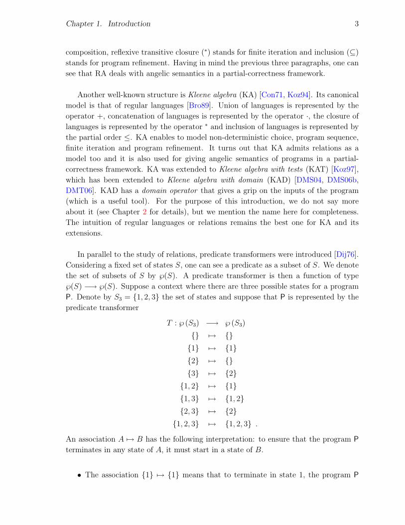
In parallel to the study of relations, predicate transformers were introduced [Dij76].
Considering a fixed set of states S, one can see a predicate as a subset of S. We denote
the set of subsets of S by ℘(S). A predicate transformer is then a function of type
℘(S) −→ ℘(S). Suppose a context where there are three possible states for a program
P. Denote by S3 = {1, 2, 3} the set of states and suppose that P is represented by the
predicate transformer
T : ℘ (S3) −→ ℘ (S3)
{} 7→ {}{1} 7→ {1}{2} 7→ {}{3} 7→ {2}
{1, 2} 7→ {1}{1, 3} 7→ {1, 2}{2, 3} 7→ {2}
{1, 2, 3} 7→ {1, 2, 3} .
An association A 7→ B has the following interpretation: to ensure that the program P
terminates in any state of A, it must start in a state of B.
• The association {1} 7→ {1} means that to terminate in state 1, the program P
Chapter 1. Introduction 4
must start in state 1.
• The association {2} 7→ {} means that there is no state from which the program
P necessarily goes to state 2.
• The association {2, 3} 7→ {2} means that to terminate in either of states 2 or 3,
the program P must start in state 2.
• The association {1, 3} 7→ {1, 2} means that to terminate in either of states 1 or
3, the program P must start either in state 1 or 2.
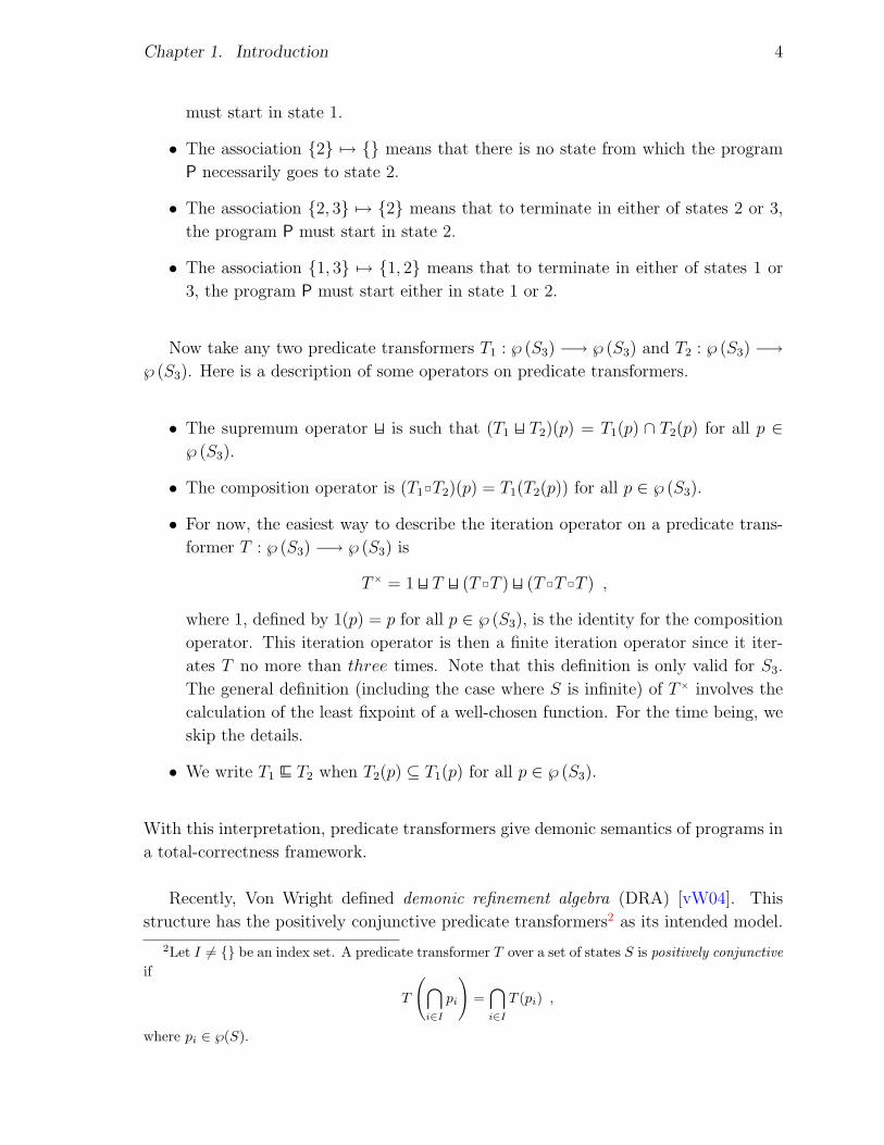
Now take any two predicate transformers T1 : ℘ (S3) −→ ℘ (S3) and T2 : ℘ (S3) −→℘ (S3). Here is a description of some operators on predicate transformers.
• The supremum operator H is such that (T1 H T2)(p) = T1(p) ∩ T2(p) for all p ∈℘ (S3).
• The composition operator is (T12T2)(p) = T1(T2(p)) for all p ∈ ℘ (S3).
• For now, the easiest way to describe the iteration operator on a predicate trans-
former T : ℘ (S3) −→ ℘ (S3) is
T× = 1 H T H (T 2T ) H (T 2T 2T ) ,
where 1, defined by 1(p) = p for all p ∈ ℘ (S3), is the identity for the composition
operator. This iteration operator is then a finite iteration operator since it iter-
ates T no more than three times. Note that this definition is only valid for S3.
The general definition (including the case where S is infinite) of T× involves the
calculation of the least fixpoint of a well-chosen function. For the time being, we
skip the details.
• We write T1 E T2 when T2(p) ⊆ T1(p) for all p ∈ ℘ (S3).
With this interpretation, predicate transformers give demonic semantics of programs in
a total-correctness framework.
Recently, Von Wright defined demonic refinement algebra (DRA) [vW04]. This
structure has the positively conjunctive predicate transformers2 as its intended model.
2Let I 6= {} be an index set. A predicate transformer T over a set of states S is positively conjunctiveif
T
(⋂i∈I
pi
)=⋂i∈I
T (pi) ,
where pi ∈ ℘(S).

Chapter 1. Introduction 5
In addition to the finite iteration operator, it includes an infinite iteration operator ω
related to the calculation of the greatest fixpoint of a well-chosen function. DRA has
been extended to demonic refinement algebra with enabledness (DRAe) [Sol07, SvW06].
The name of this operator (enabledness operator) reflects its semantic interpretation
in the realm of programs and its axiomatisation is inspired by that of the domain
operator of KAD. For the purpose of this introduction, we do not say more about it
(see [DD06c, DD08b, Sol07, SvW06] for details or Section 6.2 for a brief presentation).
The intuition of positively conjunctive predicate transformers remains the best one for
DRA and DRAe.
1.2 The Meeting Point of Two Parallel Lines
Relations and predicate transformers seem to be the “opposite” of each other. Relations
represent an angelic semantics of programs in a partial-correctness framework and they
model the states where a program may go from a given state. Predicate transformers
represent a demonic semantics of programs in a total-correctness framework and they
model the states from which a program is guaranteed to get to a given state.
However, work has been done to bring together angelic and demonic semantics.
For instance, demonic operators were defined in RA from the angelic ones [BvdW93,
BZ86, DBS+95, DMN97, Kah01, Mad96, TD99]. Demonic operators were defined from
the angelic ones in KAD too [DMT00, DMT06]. It is worth mentioning since, as said
previously, relations are also a model of KAD. Other works relating angelic and demonic
semantics have been published [BvW92, MCR07, Sol07]. At the moment, no algebraic
structure has relations with demonic operators (or KAD with demonic operators) as its
intended model.
It turns out that relations and predicate transformers can be connected. Take
S2 = {1, 2}. The lattice of relations over S2 has the shape of the one of Figure 1.1.
This lattice might be seen as a model of RA as well as a model of KAD. By ordering
the same relations but with demonic refinement (which can be defined from the angelic
operators in RA), one gets a semilattice of the shape of the one of Figure 1.2. As
mentioned before, no algebraic structure has relations with demonic operators as its
intended model. The lattice of positively conjunctive predicate transformers over S2
has the shape of the one of Figure 1.3. This lattice might be seen as a model of DRAe.
Looking carefully at these three semilattices, one can gather them in the lattice of
Figure 1.4.

Chapter 1. Introduction 6
•
oooooooooooooooooooooo
����
����
����
�
????
????
????
?
OOOOOOOOOOOOOOOOOOOOOO
•
����
����
����
�
????
????
????
? •
oooooooooooooooooooooo
OOOOOOOOOOOOOOOOOOOOOO
TTTTTTTTTTTTTTTTTTTTTTTTTTTTTTTTT •
jjjjjjjjjjjjjjjjjjjjjjjjjjjjjjjjj
OOOOOOOOOOOOOOOOOOOOOO •
jjjjjjjjjjjjjjjjjjjjjjjjjjjjjjjjj
????
????
????
?
•
????
????
????
?
OOOOOOOOOOOOOOOOOOOOOO •
TTTTTTTTTTTTTTTTTTTTTTTTTTTTTTTTT •
OOOOOOOOOOOOOOOOOOOOOO •
jjjjjjjjjjjjjjjjjjjjjjjjjjjjjjjjj
????
????
????
? •
jjjjjjjjjjjjjjjjjjjjjjjjjjjjjjjjj •
oooooooooooooooooooooo
����
����
����
�
•
OOOOOOOOOOOOOOOOOOOOOO •
????
????
????
? •
����
����
����
�•
oooooooooooooooooooooo
•
Figure 1.1: Lattice of relations over S2 ordered by angelic refinement.
•
����
����
����
�
????
????
????
?
•
����
����
����
�
????
????
????
? •
����
����
����
�
????
????
????
?
• • •
oooooooooooooooooooooo
����
����
����
�
????
????
????
?
OOOOOOOOOOOOOOOOOOOOOO • •
•
????
????
????
? •
OOOOOOOOOOOOOOOOOOOOOO
TTTTTTTTTTTTTTTTTTTTTTTTTTTTTTTTT •
jjjjjjjjjjjjjjjjjjjjjjjjjjjjjjjjj •
jjjjjjjjjjjjjjjjjjjjjjjjjjjjjjjjj
• • • •
Figure 1.2: Lattice of relations over S2 ordered by demonic refinement.

Chapter 1. Introduction 7
•
•
�������������•
?????????????
•
�������������• •
?????????????
�������������• •
?????????????
•
�������������
oooooooooooooooooooooo •
oooooooooooooooooooooo •
�������������•
?????????????•
OOOOOOOOOOOOOOOOOOOOOO •
?????????????
OOOOOOOOOOOOOOOOOOOOOO
•
�������������
oooooooooooooooooooooo •
jjjjjjjjjjjjjjjjjjjjjjjjjjjjjjjjj •
?????????????
jjjjjjjjjjjjjjjjjjjjjjjjjjjjjjjjj •
OOOOOOOOOOOOOOOOOOOOOO •
TTTTTTTTTTTTTTTTTTTTTTTTTTTTTTTTT •
OOOOOOOOOOOOOOOOOOOOOO
?????????????
•
?????????????
jjjjjjjjjjjjjjjjjjjjjjjjjjjjjjjjj •
OOOOOOOOOOOOOOOOOOOOOO
jjjjjjjjjjjjjjjjjjjjjjjjjjjjjjjjj •
TTTTTTTTTTTTTTTTTTTTTTTTTTTTTTTTT
OOOOOOOOOOOOOOOOOOOOOO
oooooooooooooooooooooo •
?????????????
�������������
•
OOOOOOOOOOOOOOOOOOOOOO
?????????????
�������������
oooooooooooooooooooooo
Figure 1.3: Lattice of positively conjunctive predicate transformers over S2 ordered by
E.
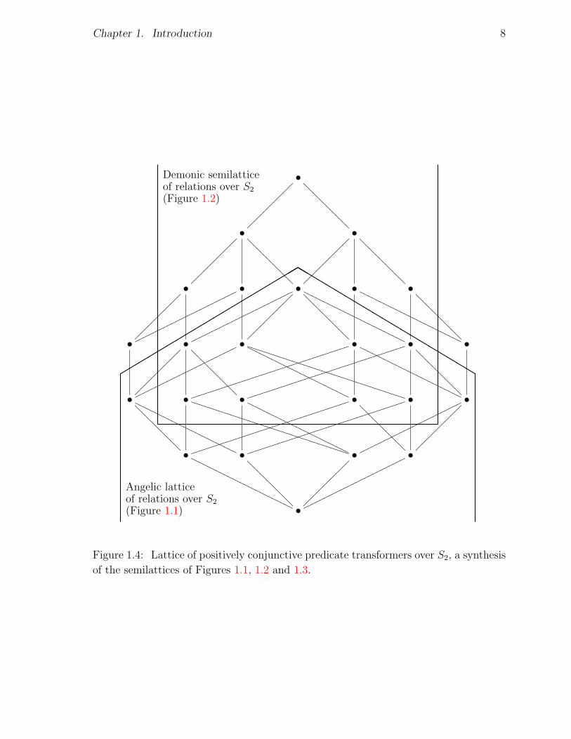
Chapter 1. Introduction 8
•
•
��������������•
??????????????
•
��������������• •
??????????????
��������������• •
??????????????
•
��������������
ooooooooooooooooooooooooo •
ooooooooooooooooooooooooo •
��������������•
??????????????•
OOOOOOOOOOOOOOOOOOOOOOOOO •
??????????????
OOOOOOOOOOOOOOOOOOOOOOOOO
•
��������������
ooooooooooooooooooooooooo •
jjjjjjjjjjjjjjjjjjjjjjjjjjjjjjjjjjjj •
??????????????
jjjjjjjjjjjjjjjjjjjjjjjjjjjjjjjjjjjj •
OOOOOOOOOOOOOOOOOOOOOOOOO •
TTTTTTTTTTTTTTTTTTTTTTTTTTTTTTTTTTTT •
OOOOOOOOOOOOOOOOOOOOOOOOO
??????????????
•
??????????????
jjjjjjjjjjjjjjjjjjjjjjjjjjjjjjjjjjjj •
OOOOOOOOOOOOOOOOOOOOOOOOO
jjjjjjjjjjjjjjjjjjjjjjjjjjjjjjjjjjjj •
TTTTTTTTTTTTTTTTTTTTTTTTTTTTTTTTTTTT
OOOOOOOOOOOOOOOOOOOOOOOOO
ooooooooooooooooooooooooo •
??????????????
��������������
•
OOOOOOOOOOOOOOOOOOOOOOOOO
??????????????
��������������
ooooooooooooooooooooooooo
""
""
""
""
""
""
""
""
""
""
bb
bb
bb
bb
bb
bb
bb
bb
bb
bb
Demonic semilatticeof relations over S2
(Figure 1.2)
Angelic latticeof relations over S2
(Figure 1.1)
Figure 1.4: Lattice of positively conjunctive predicate transformers over S2, a synthesis
of the semilattices of Figures 1.1, 1.2 and 1.3.
Chapter 1. Introduction 9
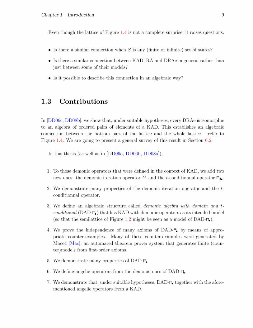
Even though the lattice of Figure 1.4 is not a complete surprise, it raises questions.
• Is there a similar connection when S is any (finite or infinite) set of states?
• Is there a similar connection between KAD, RA and DRAe in general rather than
just between some of their models?
• Is it possible to describe this connection in an algebraic way?
1.3 Contributions
In [DD06c, DD08b], we show that, under suitable hypotheses, every DRAe is isomorphic
to an algebra of ordered pairs of elements of a KAD. This establishes an algebraic
connection between the bottom part of the lattice and the whole lattice —refer to
Figure 1.4. We are going to present a general survey of this result in Section 6.2.
In this thesis (as well as in [DD06a, DD06b, DD08a]),
1. To those demonic operators that were defined in the context of KAD, we add two
new ones: the demonic iteration operator ×A and the t-conditionnal operator GA•.
2. We demonstrate many properties of the demonic iteration operator and the t-
conditionnal operator.
3. We define an algebraic structure called demonic algebra with domain and t-
conditional (DAD-G•) that has KAD with demonic operators as its intended model
(so that the semilattice of Figure 1.2 might be seen as a model of DAD-G•).
4. We prove the independence of many axioms of DAD-G• by means of appro-
priate counter-examples. Many of these counter-examples were generated by
Mace4 [Mac], an automated theorem prover system that generates finite (coun-
ter)models from first-order axioms.
5. We demonstrate many properties of DAD-G•.
6. We define angelic operators from the demonic ones of DAD-G•.
7. We demonstrate that, under suitable hypotheses, DAD-G• together with the afore-
mentioned angelic operators form a KAD.
Chapter 1. Introduction 10
KAD
DAD-G•
DAD-G•with
decomposableelements
@@RF
@@IG
Figure 1.5: Representation of the duality between KAD and DAD-G•.
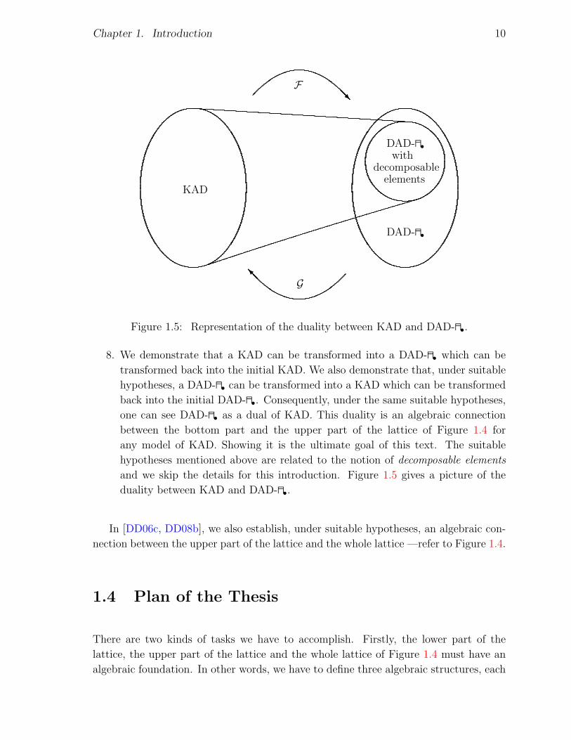
8. We demonstrate that a KAD can be transformed into a DAD-G• which can be
transformed back into the initial KAD. We also demonstrate that, under suitable
hypotheses, a DAD-G• can be transformed into a KAD which can be transformed
back into the initial DAD-G•. Consequently, under the same suitable hypotheses,
one can see DAD-G• as a dual of KAD. This duality is an algebraic connection
between the bottom part and the upper part of the lattice of Figure 1.4 for
any model of KAD. Showing it is the ultimate goal of this text. The suitable
hypotheses mentioned above are related to the notion of decomposable elements
and we skip the details for this introduction. Figure 1.5 gives a picture of the
duality between KAD and DAD-G•.
In [DD06c, DD08b], we also establish, under suitable hypotheses, an algebraic con-
nection between the upper part of the lattice and the whole lattice —refer to Figure 1.4.
1.4 Plan of the Thesis
There are two kinds of tasks we have to accomplish. Firstly, the lower part of the
lattice, the upper part of the lattice and the whole lattice of Figure 1.4 must have an
algebraic foundation. In other words, we have to define three algebraic structures, each

Chapter 1. Introduction 11
one of them having one part of the lattice as its intended model. KAD is an algebraic
foundation for the lower part, DAD-G• is an algebraic foundation for the upper part,
and DRAe is an algebraic foundation for the whole lattice. Secondly, we have to define
transformations from any part of the lattice to any other part of the lattice. In this
thesis, we mainly concentrate on the bottom part and the upper part. The treatment
of the whole lattice will only be skimmed over.
Here is how the thesis is divided. At first, in Chapter 2, we recall the definitions of
Kleene algebra (KA) and its extensions, Kleene algebra with tests (KAT) and Kleene
algebra with domain (KAD). This chapter also contains the definitions of the usual
demonic operators in terms of the KAD’s operators. To these operators, we add two
new demonic ones and we derive new simple results about all of them. The chapter
concludes with a fundamental theorem stating that the elements of a KAD together with
the demonic operators form a demonic algebra with domain and t-conditional (defined
in the following chapter). It is the first step toward the desired duality.
Secondly, in Chapter 3, we present a new structure called demonic algebra (DA) and
its extensions, demonic algebra with tests (DAT), demonic algebra with domain (DAD)
and demonic algebra with domain and t-conditional (DAD-G•). We also demonstrate
many results about these structures.
Thirdly, in Chapter 4, we define angelic operators from DAD-G•’s operators. In
order to do so, we need to define decomposable elements. These are indispensable for the
definition of angelic composition. Once angelic operators are defined, we present major
results about them and about decomposable elements. The chapter concludes with
a fundamental theorem stating that the decomposable elements of a DAD-G• together
with the angelic operators form a KAD. It is the second step toward the desired duality.
Then, in Chapter 5, we define —refer to Figure 1.5— functions F and G such that
F(K) is a DAD-G• for each KAD K and, under suitable conditions, G(A) is a KAD
for each DAD-G• A. Then, we demonstrate that (under the same suitable conditions)
G ◦ F is the identity on any KAD K and F ◦ G is the identity on any DAD-G• A. It is
the third and last step toward the desired duality.
In Chapter 6, we present a short discussion about two different algebras of ordered
pairs. The first algebra helps understand models of DAD-G•. The second one was
defined in [DD06c, DD08b] and it is behind an algebraic connection between the bottom
part of the lattice and the whole lattice of Figure 1.4.
We finally conclude in Chapter 7.

Chapter 2
Kleene Algebra with Domain and
KAD-based Demonic Operators
We explained in the introduction that the ultimate goal of this thesis is to establish an
algebraic connection —a duality— between the lower part and the upper part of the
lattice of Figure 1.4. In order to do so, we need an algebraic description of each part.
In this chapter, we present algebraic foundations for the lower part of the lattice of
Figure 1.4. Indeed, we recall basic definitions about Kleene algebra (KA) (Section 2.1)
and its extensions, Kleene algebra with tests (KAT) (Section 2.2) and Kleene algebra
with domain (KAD) (Section 2.3).
Then we present the KAD-based definition of the demonic operators (Section 2.4)
together with crucial properties they satisfy (Section 2.5). It prepares the ground for
Chapter 3 where we present algebraic foundations for the upper part of the lattice of
Figure 1.4. It is the first step toward the desired duality (refer to Section 1.3).
2.1 Kleene Algebra
In this section, we present the concept of Kleene algebra (KA) and we discuss some of
its axioms. Initially, different variants of KA were introduced by Conway [Con71], but
since then, one of them has become well known, thanks to Kozen [Koz94]. This is the
one we present in this section and use throughout this thesis.
Chapter 2. Kleene Algebra with Domain and KAD-based Demonic Operators 13
Definition 2.1 (Kleene algebra). A Kleene algebra (KA) is a structure K = (K,+, ·, ∗,0, 1) such that the following properties hold for all x, y, z ∈ K.
(x+ y) + z = x+ (y + z) (2.1)
x+ y = y + x (2.2)
x+ x = x (2.3)
0 + x = x (2.4)
(x · y) · z = x · (y · z) (2.5)
0 · x = x · 0 = 0 (2.6)
1 · x = x · 1 = x (2.7)
x · (y + z) = x · y + x · z (2.8)
(x+ y) · z = x · z + y · z (2.9)
x∗ = x∗ · x+ 1 (2.10)
Addition induces a partial order ≤ such that, for all x, y ∈ K,
x ≤ y ⇐⇒ x+ y = y . (2.11)
Finally, the following properties must be satisfied for all x, y, z ∈ K.
x · z + y ≤ z =⇒ x∗ · y ≤ z (2.12)
z · x+ y ≤ z =⇒ y · x∗ ≤ z (2.13)
Remark 2.2. Hollenberg has shown that the following symmetric version of (2.10),
x∗ = x · x∗ + 1 , (2.14)
is derivable from these axioms [Hol96]. The converse is true. Indeed, if (2.10) were re-
placed by (2.14) in the axiomatisation of KA, then (2.10) would be derivable from these
axioms. Moreover, Kozen has shown in [Koz90] that (2.12) and (2.13) are independent.
Also, one can show x∗ = µ≤(y :: y · x + 1) with (2.7), (2.10) and (2.13), and
x∗ = µ≤(y :: x · y + 1) with (2.7), (2.14) and (2.12).
Finally, in the presence of the other axioms, (2.12) and (2.13) are equivalent to the
following two.
x · z ≤ z =⇒ x∗ · z ≤ z (2.15)
z · x ≤ z =⇒ z · x∗ ≤ z (2.16)
The natural model of KA is regular languages. However, it is the study of relational
models of KA that led us to the lattice of Figure 1.4 and inspired us for the present
work. This is why, throughout this thesis, we elude regular languages.

Chapter 2. Kleene Algebra with Domain and KAD-based Demonic Operators 14
(1 1
1 1
)
ppppppppppppppppppp
����
����
��
====
====
==
NNNNNNNNNNNNNNNNNNN
(1 1
1 0
)
����
����
��
====
====
==
(1 1
0 1
)
ppppppppppppppppppp
NNNNNNNNNNNNNNNNNNN
TTTTTTTTTTTTTTTTTTTTTTTTTTTTTTT
(1 0
1 1
)
jjjjjjjjjjjjjjjjjjjjjjjjjjjjjjj
NNNNNNNNNNNNNNNNNNN
(0 1
1 1
)
jjjjjjjjjjjjjjjjjjjjjjjjjjjjjjj
====
====
==
(1 1
0 0
)
====
====
==
NNNNNNNNNNNNNNNNNNN
(1 0
1 0
)
TTTTTTTTTTTTTTTTTTTTTTTTTTTTTTT
(0 1
1 0
)
NNNNNNNNNNNNNNNNNNN
(1 0
0 1
)
jjjjjjjjjjjjjjjjjjjjjjjjjjjjjjj
====
====
==
(0 1
0 1
)
jjjjjjjjjjjjjjjjjjjjjjjjjjjjjjj
(0 0
1 1
)
ppppppppppppppppppp
����
����
��
(1 0
0 0
)
NNNNNNNNNNNNNNNNNNN
(0 1
0 0
)
====
====
==
(0 0
1 0
)
����
����
��
(0 0
0 1
)
ppppppppppppppppppp
(0 0
0 0
)
Figure 2.1: Relation algebra over the set S2 ordered by ⊆.
Consider the relations over the set S2 = {1, 2}. Interpreting + as union (∪), · as
composition of relations (;), ∗ as reflexive transitive closure, 0 as {}, 1 as {(1, 1), (2, 2)}and ≤ as inclusion (⊆), one gets a model of KA. Figure 2.1 displays the Boolean matrix
representation of the lattice of these relations ordered by ⊆. It is a more detailed version
of Figure 1.1.
2.2 Kleene Algebra with Tests
KA, as defined in the previous section, is itself an algebraic foundation of the lower
part of the lattice of Figure 1.4. However, as we mentioned earlier, we want to define
demonic operators in the context of KA. For this matter (see Section 2.4), we need a
domain operator that cannot be defined without the concept of test.
Of course, at first, the purpose of tests was not to define a domain operator. His-
Chapter 2. Kleene Algebra with Domain and KAD-based Demonic Operators 15
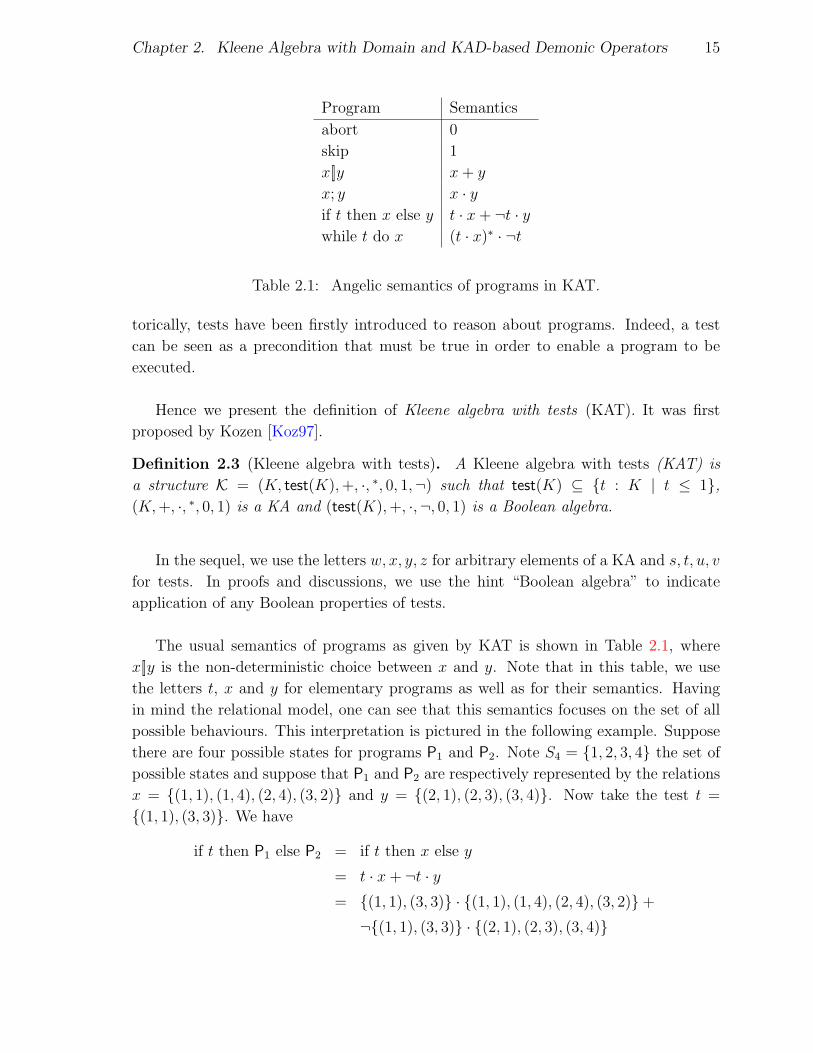
Program Semantics
abort 0
skip 1
x[]y x+ y
x; y x · yif t then x else y t · x+ ¬t · ywhile t do x (t · x)∗ · ¬t
Table 2.1: Angelic semantics of programs in KAT.
torically, tests have been firstly introduced to reason about programs. Indeed, a test
can be seen as a precondition that must be true in order to enable a program to be
executed.
Hence we present the definition of Kleene algebra with tests (KAT). It was first
proposed by Kozen [Koz97].
Definition 2.3 (Kleene algebra with tests). A Kleene algebra with tests (KAT) is
a structure K = (K, test(K),+, ·, ∗, 0, 1,¬) such that test(K) ⊆ {t : K | t ≤ 1},(K,+, ·, ∗, 0, 1) is a KA and (test(K),+, ·,¬, 0, 1) is a Boolean algebra.
In the sequel, we use the letters w, x, y, z for arbitrary elements of a KA and s, t, u, v
for tests. In proofs and discussions, we use the hint “Boolean algebra” to indicate
application of any Boolean properties of tests.
The usual semantics of programs as given by KAT is shown in Table 2.1, where
x[]y is the non-deterministic choice between x and y. Note that in this table, we use
the letters t, x and y for elementary programs as well as for their semantics. Having
in mind the relational model, one can see that this semantics focuses on the set of all
possible behaviours. This interpretation is pictured in the following example. Suppose
there are four possible states for programs P1 and P2. Note S4 = {1, 2, 3, 4} the set of
possible states and suppose that P1 and P2 are respectively represented by the relations
x = {(1, 1), (1, 4), (2, 4), (3, 2)} and y = {(2, 1), (2, 3), (3, 4)}. Now take the test t =
{(1, 1), (3, 3)}. We have
if t then P1 else P2 = if t then x else y
= t · x+ ¬t · y= {(1, 1), (3, 3)} · {(1, 1), (1, 4), (2, 4), (3, 2)}+
¬{(1, 1), (3, 3)} · {(2, 1), (2, 3), (3, 4)}
Chapter 2. Kleene Algebra with Domain and KAD-based Demonic Operators 16
= {(1, 1), (3, 3)} · {(1, 1), (1, 4), (2, 4), (3, 2)}+
{(2, 2), (4, 4)} · {(2, 1), (2, 3), (3, 4)}= {(1, 1), (1, 4), (3, 2)}+ {(2, 1), (2, 3)}= {(1, 1), (1, 4), (2, 1), (2, 3), (3, 2)}
which is the set of all possible behaviours. It is now easy to see that the semantics
presented in Table 2.1 are angelic ones.
2.3 Kleene Algebra with Domain
It is useful to have a grip on the inputs of the aforementioned programs. The domain
operator encapsulates the necessary properties. Moreover, it is an essential operator in
the definition of demonic operators in the context of KA (see Section 2.4).
Here is the definition of Kleene algebra with domain (KAD) as defined by Desharnais,
Moller, Struth and Tchier [DMS04, DMS06b, DMT06].
Definition 2.4 (Kleene algebra with domain). A Kleene algebra with domain (KAD)
is a structure K = (K, test(K),+, ·, ∗, 0, 1,¬, p ) such that (K, test(K),+, ·, ∗, 0, 1,¬) is
a KAT and, for all x ∈ K and all t ∈ test(K),
x ≤ px · x , (2.17)
p(t · x) ≤ t , (2.18)
p(x · py) ≤ p(x · y) . (2.19)
Remark 2.5. It turns out that these axioms force the test algebra test(K) to be the
maximal Boolean algebra included in {t : K | t ≤ 1} (see [DMS06b]).
Note that (2.19) is satisfied for relation algebras1. It is called locality . However,
there are KATs where it does not hold. Indeed, the following counter-example appears
in [DM01].
Example 2.6. Take K = {0, 1, a, b} and test(K) = {0, 1}. The operators defined by
the following tables make (K, test(K),+, ·, ∗, 0, 1,¬) a KAT.
+ 0 1 a b
0 0 1 a b
1 1 1 b b
a a b a b
b b b b b
· 0 1 a b
0 0 0 0 0
1 0 1 a b
a 0 a 0 a
b 0 b a b
∗
0 1
1 1
a b
b b
¬0 1
1 0
p
0 0
1 1
a 1
b 1
1For a relation R on a set S, pR = {(s, s) : S × S | (∃ t : S | (s, t) ∈ R)}.
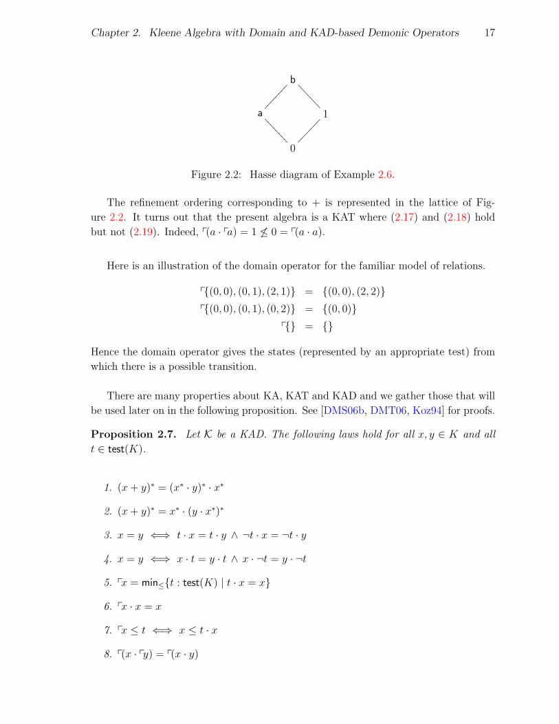
Chapter 2. Kleene Algebra with Domain and KAD-based Demonic Operators 17
b
����
����
====
===
a
====
==== 1
����
���
0
Figure 2.2: Hasse diagram of Example 2.6.
The refinement ordering corresponding to + is represented in the lattice of Fig-
ure 2.2. It turns out that the present algebra is a KAT where (2.17) and (2.18) hold
but not (2.19). Indeed, p(a · pa) = 1 6≤ 0 = p(a · a).
Here is an illustration of the domain operator for the familiar model of relations.
p{(0, 0), (0, 1), (2, 1)} = {(0, 0), (2, 2)}p{(0, 0), (0, 1), (0, 2)} = {(0, 0)}
p{} = {}
Hence the domain operator gives the states (represented by an appropriate test) from
which there is a possible transition.
There are many properties about KA, KAT and KAD and we gather those that will
be used later on in the following proposition. See [DMS06b, DMT06, Koz94] for proofs.
Proposition 2.7. Let K be a KAD. The following laws hold for all x, y ∈ K and all
t ∈ test(K).
1. (x+ y)∗ = (x∗ · y)∗ · x∗
2. (x+ y)∗ = x∗ · (y · x∗)∗
3. x = y ⇐⇒ t · x = t · y ∧ ¬t · x = ¬t · y
4. x = y ⇐⇒ x · t = y · t ∧ x · ¬t = y · ¬t
5. px = min≤{t : test(K) | t · x = x}
6. px · x = x
7. px ≤ t ⇐⇒ x ≤ t · x
8. p(x · py) = p(x · y)

Chapter 2. Kleene Algebra with Domain and KAD-based Demonic Operators 18
9. ¬px · x = 0
10. pt = t
11. p(t · x) = t · px
12. p(x · y) ≤ px
13. p(x+ y) = px+ py
14. x ≤ y =⇒ px ≤ py
15. p(x · t) ≤ t ⇐⇒ p(x∗ · t) ≤ t
16. p(x∗) = 1
The following operator characterises the set of states from which no computation
as described by x may lead outside the domain of y. It facilitates the presentation and
the comprehension of further definitions and results.
Definition 2.8 (KA-implication). Let K be a KAD and take x, y ∈ K. The KA-
implication x→ y is defined by
x→ y = ¬p(x · ¬py) .
2.4 KAD-Based Demonic Operators
We are now ready to introduce demonic operators in the context of KAD. What do
we need them for? When we constructed the upper part of the lattice displayed in
Figure 1.4 in the introduction, we took the elements of the bottom part of the same
lattice and we (partially-)ordered them by demonic refinement. Those elements are
relations and it is possible to define not only demonic refinement on them, but many
demonic operators (see [BvdW93, BZ86, DBS+95, DMN97, Kah01, Mad96, TD99]).
What we are trying to develop is an algebraic description of the lattice of Figure 1.4
and of its connections, but for any model of KAD. Therefore, we need to look at the
definition of demonic operators, but from now, in the context of KAD. Most of them
were defined in [DMT00, DMT06].
Here is the definition of demonic refinement.
Chapter 2. Kleene Algebra with Domain and KAD-based Demonic Operators 19
Definition 2.9 (Demonic refinement). Let K be a KAD and take x, y ∈ K. We say
that x refines y, noted x EA y, when
py ≤ px ,
py · x ≤ y .
The subscript A in EA indicates that the demonic refinement is defined with the
operators of the angelic world. An analogous notation will be introduced when we
define angelic operators in the demonic world.
This definition can be simply illustrated with relations. Let Q = {(1, 2), (2, 4)}and R = {(1, 2), (1, 3)}. Then pR = {(1, 1)} ⊆ {(1, 1), (2, 2)} = pQ. Since in addition
pR ·Q = {(1, 2)} ⊆ R, we have Q EA R.
The following proposition helps understand the definition of EA (see [DMT06] for
proof).
Proposition 2.10 (Demonic upper semilattice).
1. The relation EA defined in KAD is a partial order and it induces an upper semi-
lattice with demonic join HA:
x EA y ⇐⇒ x HA y = y .
2. Demonic join satisfies the following two properties.
x HA y = px · py · (x+ y)
p(x HA y) = px HA py = px · py
Remark 2.11. Note that for all s, t ∈ test(K),
s EA t ⇐⇒ t ≤ s .
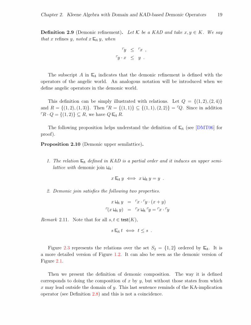
Figure 2.3 represents the relations over the set S2 = {1, 2} ordered by EA. It is
a more detailed version of Figure 1.2. It can also be seen as the demonic version of
Figure 2.1.
Then we present the definition of demonic composition. The way it is defined
corresponds to doing the composition of x by y, but without those states from which
x may lead outside the domain of y. This last sentence reminds of the KA-implication
operator (see Definition 2.8) and this is not a coincidence.
Chapter 2. Kleene Algebra with Domain and KAD-based Demonic Operators 20
(0 0
0 0
)
{{{{
{{{{
{
CCCC
CCCC
C
(0 0
1 1
)
{{{{
{{{{
{
CCCC
CCCC
C
(1 1
0 0
)
{{{{
{{{{
{
CCCC
CCCC
C
(0 0
1 0
) (0 0
0 1
) (1 1
1 1
)
mmmmmmmmmmmmmmmmmmmmm
{{{{
{{{{
{
CCCC
CCCC
C
QQQQQQQQQQQQQQQQQQQQQ
(1 0
0 0
) (0 1
0 0
)
(1 1
1 0
)
CCCC
CCCC
C
(1 1
0 1
)
QQQQQQQQQQQQQQQQQQQQQ
VVVVVVVVVVVVVVVVVVVVVVVVVVVVVVVVVVV
(1 0
1 1
)
hhhhhhhhhhhhhhhhhhhhhhhhhhhhhhhhhhh
(0 1
1 1
)
hhhhhhhhhhhhhhhhhhhhhhhhhhhhhhhhhhh
(1 0
1 0
) (0 1
1 0
) (1 0
0 1
) (0 1
0 1
)
Figure 2.3: Relation algebra over the set S2 = {1, 2} ordered by EA.
Definition 2.12 (Demonic composition). Let K be a KAD and take x, y ∈ K. The
demonic composition of x and y, written x 2A y, is defined by
x 2A y = (x→ y) · x · y .
Again using relations, we illustrate this definition. Let Q = {(1, 2), (1, 4), (2, 3),
(4, 1)}, R = {(1, 1), (2, 4)} and suppose the state space is S4 = {1, 2, 3, 4}. Then
Q→ R = {(1, 2), (1, 4), (2, 3), (4, 1)} → {(1, 1), (2, 4)}= ¬p({(1, 2), (1, 4), (2, 3), (4, 1)} · ¬p{(1, 1), (2, 4)})= ¬p({(1, 2), (1, 4), (2, 3), (4, 1)} · ¬{(1, 1), (2, 2)})= ¬p({(1, 2), (1, 4), (2, 3), (4, 1)} · {(3, 3), (4, 4)})= ¬p{(1, 4), (2, 3)}= ¬{(1, 1), (2, 2)}= {(3, 3), (4, 4)}
so
Q 2A R = (Q→ R) ·Q ·R

Chapter 2. Kleene Algebra with Domain and KAD-based Demonic Operators 21
= {(3, 3), (4, 4)} · {(1, 2), (1, 4), (2, 3), (4, 1)} · {(1, 1), (2, 4)}= {(3, 3), (4, 4)} · {(1, 4), (4, 1)}= {(4, 1)} .
There are many properties about KA-implication and demonic composition and
we gather those that will be used later on in the following proposition. See [DMT00,
DMT06] for proofs.
Proposition 2.13. Let K be a KAD. The following laws hold for all x, y, z ∈ K and
all t ∈ test(K).
1. x 2A (y 2A z) = (x 2A y) 2A z
2. t 2A x = t · x
3. py = 1 =⇒ x 2A y = x · y
4. p(x 2A y) = (x→ y) · px
5. x→ y = x→ py
6. (x→ y) · x = (x→ y) · x · py
7. (x · y) → z = x→ (y → z)
8. t ≤ x→ t ⇐⇒ t ≤ x∗ → t
9. x ≤ y =⇒ y → z ≤ x→ z
10. y ≤ z =⇒ x→ y ≤ x→ z
11. x 2A y ≤ x · y
12. x EA y =⇒ x 2A z EA y 2A z
13. x EA y =⇒ z 2A x EA z 2A y
In this section, we are defining a demonic version of the usual operators of KAD.
Knowing that x∗ = µ≤(y :: y · x + 1) (see Remark 2.2), the demonic version of the
Kleene star ought to be x×A = µEA(y :: y 2A x HA 1). This is the object of the following
definition, lemma and proposition.
Definition 2.14 (Demonic iteration operator). Let K be a KAD and take x ∈ K. The
demonic iteration operator ×A is defined by x×A = x∗ 2A px.

Chapter 2. Kleene Algebra with Domain and KAD-based Demonic Operators 22
Lemma 2.15. Let K be a KAD and take x ∈ K. Then
p(x×A) = x∗ → px .
Proof :
p(x×A)
= 〈 by Definition 2.14 〉
p(x∗ 2A px)
= 〈 by Proposition 2.13-4 〉
(x∗ → px) · p(x∗)= 〈 by Proposition 2.7-16 and Boolean algebra 〉
x∗ → px
2
Proposition 2.16. Let K be a KAD and take x, y, z ∈ K.
1. x×A = x×A 2A x HA 1
2. x 2A z EA z =⇒ x×A 2A z EA z
3. z 2A x EA z =⇒ z 2A x×A EA z
4. x 2A z HA y EA z =⇒ x×A 2A y EA z
5. z 2A x HA y EA z =⇒ y 2A x×A EA z
Proof :
1. x×A 2A x HA 1
= 〈 by Definition 2.14 and Proposition 2.13-1 〉
x∗ 2A (px 2A x) HA 1
= 〈 by Propositions 2.13-2 and 2.7-6 〉
x∗ 2A x HA 1

Chapter 2. Kleene Algebra with Domain and KAD-based Demonic Operators 23
= 〈 by Propositions 2.10 and 2.7-10, and (2.7) 〉
p(x∗ 2A x) · (x∗ 2A x+ 1)
= 〈 by Proposition 2.13-4 and Definition 2.12 〉
(x∗ → x) · p(x∗) · ((x∗ → x) · x∗ · x+ 1)
= 〈 by Proposition 2.7-16 and (2.7) 〉
(x∗ → x) · ((x∗ → x) · x∗ · x+ 1)
= 〈 by (2.8) and Boolean algebra 〉
(x∗ → x) · (x∗ · x+ 1)
= 〈 by (2.10) 〉
(x∗ → x) · x∗
= 〈 by Propositions 2.13-6 and 2.7-6 〉
(x∗ → x) · x∗ · px= 〈 by Definitions 2.12 and 2.14 〉
x×A
2. x×A 2A z EA z
⇐⇒ 〈 by Definition 2.14 and Proposition 2.13-1 〉
x∗2(px 2A z) EA z
⇐⇒ 〈 by Proposition 2.13-2 〉
x∗ 2A (px · z) EA z
⇐⇒ 〈 by Definition 2.9 〉
pz ≤ p(x∗ 2A (px · z)) ∧ pz · (x∗ 2A (px · z)) ≤ z
⇐⇒ 〈 by Proposition 2.13-4 and Definition 2.12 〉
pz ≤ (x∗ → (px · z)) · p(x∗) ∧ pz · (x∗ → (px · z)) · x∗ · px · z ≤ z
⇐⇒ 〈 by Proposition 2.7-16 and (2.7) 〉
pz ≤ x∗ → (px · z) ∧ pz · (x∗ → (px · z)) · x∗ · px · z ≤ z
⇐⇒ 〈 by Boolean algebra 〉
pz ≤ x∗ → (px · z) ∧ pz · x∗ · px · z ≤ z
⇐= 〈 by Proposition 2.7-6, Boolean algebra and since pz ≤ px,z = pz · z = px · pz · z = px · z 〉
pz ≤ px ∧ pz ≤ x∗ → z ∧ pz · x∗ · z ≤ z
⇐⇒ 〈 by Proposition 2.13-5, (2.8) and Boolean algebra 〉
Chapter 2. Kleene Algebra with Domain and KAD-based Demonic Operators 24
pz ≤ px ∧ pz ≤ x∗ → pz ∧ pz · (pz · x+ ¬pz · x)∗ · z ≤ z
⇐⇒ 〈 by Propositions 2.13-8 and 2.7-1 〉
pz ≤ px ∧ pz ≤ x→ pz ∧ pz · ((pz · x)∗ · ¬pz · x)∗ · (pz · x)∗ · z ≤ z
⇐⇒ 〈 by Boolean algebra, Propositions 2.13-4 and 2.13-6,
and since pz ≤ x→ pz,pz · x = pz · (x→ pz) · x = pz · (x→ pz) · x · pz = pz · x · pz 〉
pz ≤ px ∧ pz ≤ x→ pz ∧ pz · ((pz · x · pz)∗ · ¬pz · x)∗ · (pz · x)∗ · z ≤ z
⇐⇒ 〈 by (2.10) 〉
pz ≤ px ∧ pz ≤ x→ pz ∧pz ·(((pz · x · pz)∗ · pz · x · pz + 1) · ¬pz · x
)∗· (pz · x)∗ · z ≤ z
⇐⇒ 〈 by (2.9), (2.4) and Boolean algebra 〉
pz ≤ px ∧ pz ≤ x→ pz ∧ pz · (¬pz · x)∗ · (pz · x)∗ · z ≤ z
⇐⇒ 〈 by Proposition 2.13-5 and (2.14) 〉
pz ≤ px ∧ pz ≤ x→ z ∧ pz · (¬pz · x · (¬pz · x)∗ + 1) · (pz · x)∗ · z ≤ z
⇐⇒ 〈 by (2.8), (2.4), (2.7) and Boolean algebra 〉
pz ≤ px ∧ pz ≤ x→ z ∧ pz · (pz · x)∗ · z ≤ z
⇐= 〈 by Proposition 2.7-6,
(pz · x)∗ · z ≤ z =⇒ pz · (pz · x)∗ · z ≤ z 〉pz ≤ px ∧ pz ≤ x→ z ∧ (pz · x)∗ · z ≤ z
⇐= 〈 by (2.15) 〉
pz ≤ px ∧ pz ≤ x→ z ∧ pz · x · z ≤ z
⇐⇒ 〈 by Boolean algebra 〉
pz ≤ (x→ z) · px ∧ pz · (x→ z) · x · z ≤ z
⇐⇒ 〈 by Proposition 2.13-4 and Definition 2.12 〉
pz ≤ p(x 2A z) ∧ pz · (x 2A z) ≤ z
⇐⇒ 〈 by Definition 2.9 〉
x 2A z EA z
3. z 2A x EA z
⇐⇒ 〈 by Definition 2.9 〉
pz ≤ p(z 2A x) ∧ pz · (z 2A x) ≤ z
⇐⇒ 〈 by Proposition 2.13-4 and Definition 2.12 〉
pz ≤ (z → x) · pz ∧ pz · (z → x) · z · x ≤ z

Chapter 2. Kleene Algebra with Domain and KAD-based Demonic Operators 25
⇐⇒ 〈 by Boolean algebra and Proposition 2.7-6 〉
pz ≤ (z → x) · pz ∧ z · x ≤ z
=⇒ 〈 by Proposition 2.13-5 and (2.16) 〉
pz ≤ (z → px) · pz ∧ z · x∗ ≤ z
This derivation thus gives
pz ≤ (z → px) · pz , (2.20)
z · x∗ ≤ z . (2.21)
pz
≤ 〈 by (2.20) 〉
(z → px) · pz≤ 〈 by (2.21) and Proposition 2.13-9 〉
((z · x∗) → px) · pz= 〈 by Proposition 2.13-7 〉
(z → (x∗ → px)) · pz= 〈 by Proposition 2.7-16 and (2.7) 〉
(z → ((x∗ → px) · p(x∗))) · pz= 〈 by Propositions 2.13-4 and 2.13-5 〉
(z → (x∗ 2A px)) · pz= 〈 by Proposition 2.13-4 〉
p(z 2A (x∗ 2A px))
= 〈 by Definition 2.14 〉
p(z 2A x×A)
The following inequality is also needed.
pz · (z 2A x×A)
= 〈 by Definition 2.14 〉
pz · (z 2A (x∗ 2A px))
≤ 〈 Proposition 2.12-11 〉
pz · z · (x∗ 2A px)
≤ 〈 Proposition 2.12-11 〉

Chapter 2. Kleene Algebra with Domain and KAD-based Demonic Operators 26
pz · z · x∗ · px≤ 〈 by (2.21) and because pz ≤ 1 and px ≤ 1 〉
z
The result then follows from Definition 2.9.
4. Suppose x 2A z HA y EA z. Then y EA z and x 2A z EA z by Proposition 2.10. Then
Part 2 of the present proposition gives x×A 2A z EA z. This is used in the following
derivation.
x×A 2A y
EA 〈 by the hypothesis and Proposition 2.13-13,
y EA x 2A z HA y EA z 〉x×A 2A z
EA 〈 derived above from the hypothesis 〉
z
5. The proof is similar to the previous one. 2
Based on the partial order EA, one can focus on tests and calculate the demonic
meet of tests.
Definition 2.17 (Demonic meet of tests). Let K be a KAD. For each s, t ∈ test(K),
define
s GA t = s+ t .
Remark 2.11 together with Proposition 2.10 confirm that the operator GA really is
the demonic meet of tests with respect to EA. We now define, for any test t, the t-
conditional operator GAt that generalises the demonic meet of tests to any elements of
a KAD. Since the demonic meet of x and y does not exist in general2, xGAt y is not the
demonic meet of x and y, but rather the demonic meet of t 2A x and ¬t 2A y.
Definition 2.18 (t-conditional operator). Let K be a KAD. For each x, y ∈ K and
t ∈ test(K), the t-conditional operator is defined by xGAty = t ·x+¬t ·y. The family of
t-conditional operators corresponds to a single ternary operator GA• taking as arguments
a test t and two arbitrary elements x and y.
2Indeed, look at(
1 01 0
)and
(0 10 1
)in Figure 2.3.
Chapter 2. Kleene Algebra with Domain and KAD-based Demonic Operators 27
The following proposition says that the t-conditionnal operator does generalise the
demonic meet of tests and that it calculates the demonic meet of t 2A x and ¬t2y for
any test t.
Proposition 2.19. Let K be a KAD. The following properties hold for all x, y ∈ K
and all s, t ∈ test(K).
1. 1 GAs t = s GA t
2. The demonic meet of t 2A x and ¬t 2A y with respect to EA exists and it is equal to
x GAt y.
Proof :
1. 1 GAs t
= 〈 by Definition 2.18 〉
s · 1 + ¬s · t= 〈 by Boolean algebra 〉
s+ t
= 〈 by Definition 2.17 〉
s GA t
2. We have to show that x GAt y EA t 2A x, x GAt y EA ¬t 2A y and that x GAt y is the
greatest element with these two properties.
z EA t 2A x ∧ z EA ¬t 2A y
⇐⇒ 〈 by Proposition 2.10 〉
z HA t 2A x = t 2A x ∧ z HA ¬t 2A y = ¬t 2A y
⇐⇒ 〈 by Proposition 2.13-2 〉
z HA t · x = t · x ∧ z HA ¬t · y = ¬t · y⇐⇒ 〈 by Proposition 2.10 〉
pz · p(t · x) · (z + t · x) = t · x ∧ pz · p(¬t · y) · (z + ¬t · y) = ¬t · y⇐⇒ 〈 by (2.8), Boolean algebra and Proposition 2.7-6 〉
p(t · x) · z + pz · t · x = t · x ∧ p(¬t · y) · z + pz · ¬t · y = ¬t · y⇐⇒ 〈 by (2.8), Propositions 2.7-11 and 2.7-10, Boolean algebra, (2.6)
and (2.4) 〉
Chapter 2. Kleene Algebra with Domain and KAD-based Demonic Operators 28
p(t · x) · z + p(¬t · y) · z + pz · t · x+ pz · ¬t · y = t · x+ ¬t · y⇐⇒ 〈 by (2.8) and (2.9) 〉
(p(t · x) + p(¬t · y)) · z + pz · (t · x+ ¬t · y) = t · x+ ¬t · y⇐⇒ 〈 by Proposition 2.7-13 〉
p(t · x+ ¬t · y) · z + pz · (t · x+ ¬t · y) = t · x+ ¬t · y⇐⇒ 〈 by Definition 2.18 〉
p(x GAt y) · z + pz · (x GAt y) = x GAt y
⇐⇒ 〈 by Proposition 2.7-6, Boolean algebra and (2.8) 〉
pz · p(x GAt y) · (z + (x GAt y)) = x GAt y
⇐⇒ 〈 by Proposition 2.10 〉
z EA x GAt y
We derived
z EA t 2A x ∧ z EA ¬t 2A y ⇐⇒ z EA x GAt y . (2.22)
Taking z = x GAt y in (2.22), we see that x GAt y is a lower bound of t 2A x and
¬t 2A y. Then (2.22) says that x GAt y is the greatest lower bound of t 2A x and
¬t 2A y. 2
The demonic join operator HA is used to give the semantics of demonic non-deter-
ministic choices and 2A is used for sequences. Among the interesting properties of 2A,
we cite t 2A x = t · x (Proposition 2.13-2), which says that composing a test t with an
arbitrary element x is the same in the angelic and demonic worlds, and x 2A y = x · y if
py = 1 (Proposition 2.13-3), which says that if the second element of a composition is
total, then again the angelic and demonic compositions coincide. The ternary operator
GA• is similar to the conditional choice operator / . of Hoare et al. [HHJ+87, HJ98].
It corresponds to a guarded choice with disjoint alternatives. The demonic iteration
operator ×A rejects the finite computations that go through a state from which it is
possible to reach a state where no computation is defined (e.g., due to blocking or
abnormal termination).
Chapter 2. Kleene Algebra with Domain and KAD-based Demonic Operators 29
2.5 A Framework for Demonic Algebra with Do-
main and t-Conditional Within KAD
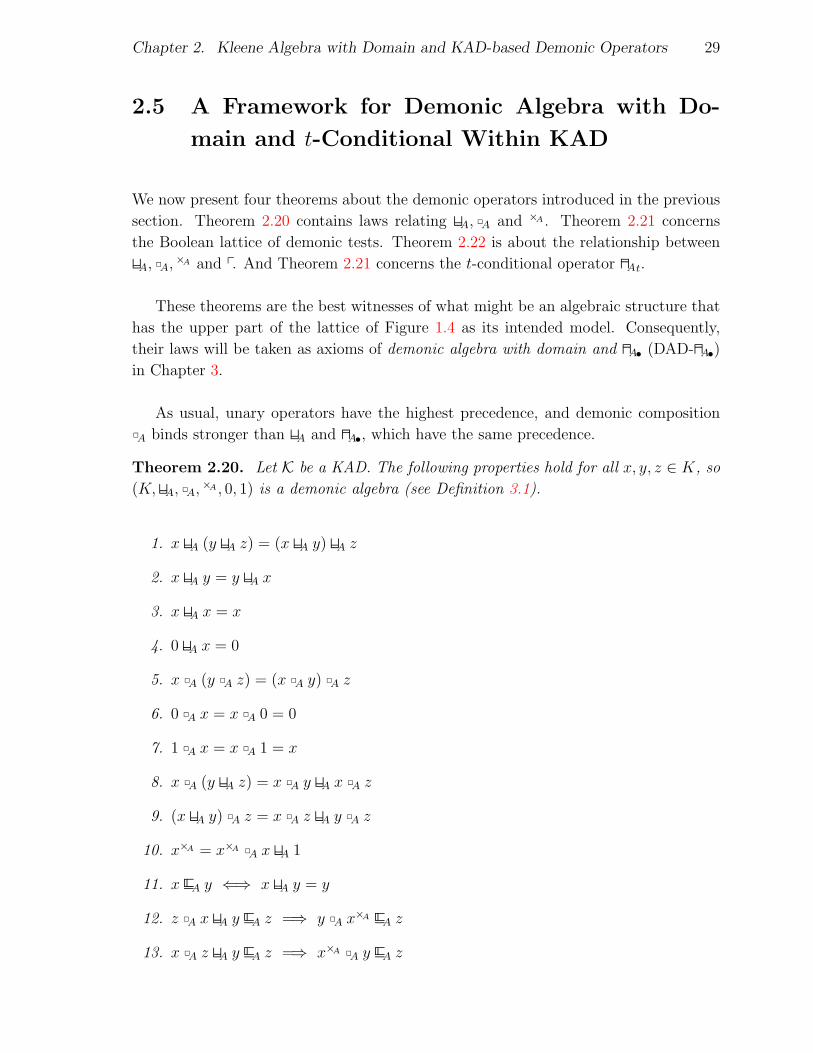
We now present four theorems about the demonic operators introduced in the previous
section. Theorem 2.20 contains laws relating HA, 2A and ×A . Theorem 2.21 concerns
the Boolean lattice of demonic tests. Theorem 2.22 is about the relationship between
HA, 2A,×A and p. And Theorem 2.21 concerns the t-conditional operator GAt.
These theorems are the best witnesses of what might be an algebraic structure that
has the upper part of the lattice of Figure 1.4 as its intended model. Consequently,
their laws will be taken as axioms of demonic algebra with domain and GA• (DAD-GA•)
in Chapter 3.
As usual, unary operators have the highest precedence, and demonic composition
2A binds stronger than HA and GA•, which have the same precedence.
Theorem 2.20. Let K be a KAD. The following properties hold for all x, y, z ∈ K, so
(K,HA, 2A,×A , 0, 1) is a demonic algebra (see Definition 3.1).
1. x HA (y HA z) = (x HA y) HA z
2. x HA y = y HA x
3. x HA x = x
4. 0 HA x = 0
5. x 2A (y 2A z) = (x 2A y) 2A z
6. 0 2A x = x 2A 0 = 0
7. 1 2A x = x 2A 1 = x
8. x 2A (y HA z) = x 2A y HA x 2A z
9. (x HA y) 2A z = x 2A z HA y 2A z
10. x×A = x×A 2A x HA 1
11. x EA y ⇐⇒ x HA y = y
12. z 2A x HA y EA z =⇒ y 2A x×A EA z
13. x 2A z HA y EA z =⇒ x×A 2A y EA z
Chapter 2. Kleene Algebra with Domain and KAD-based Demonic Operators 30
Proof : See [DMT06] for the proof of 1 to 9 and 11. Refer to Proposition 2.16 for the
proof of 10, 12 and 13. 2
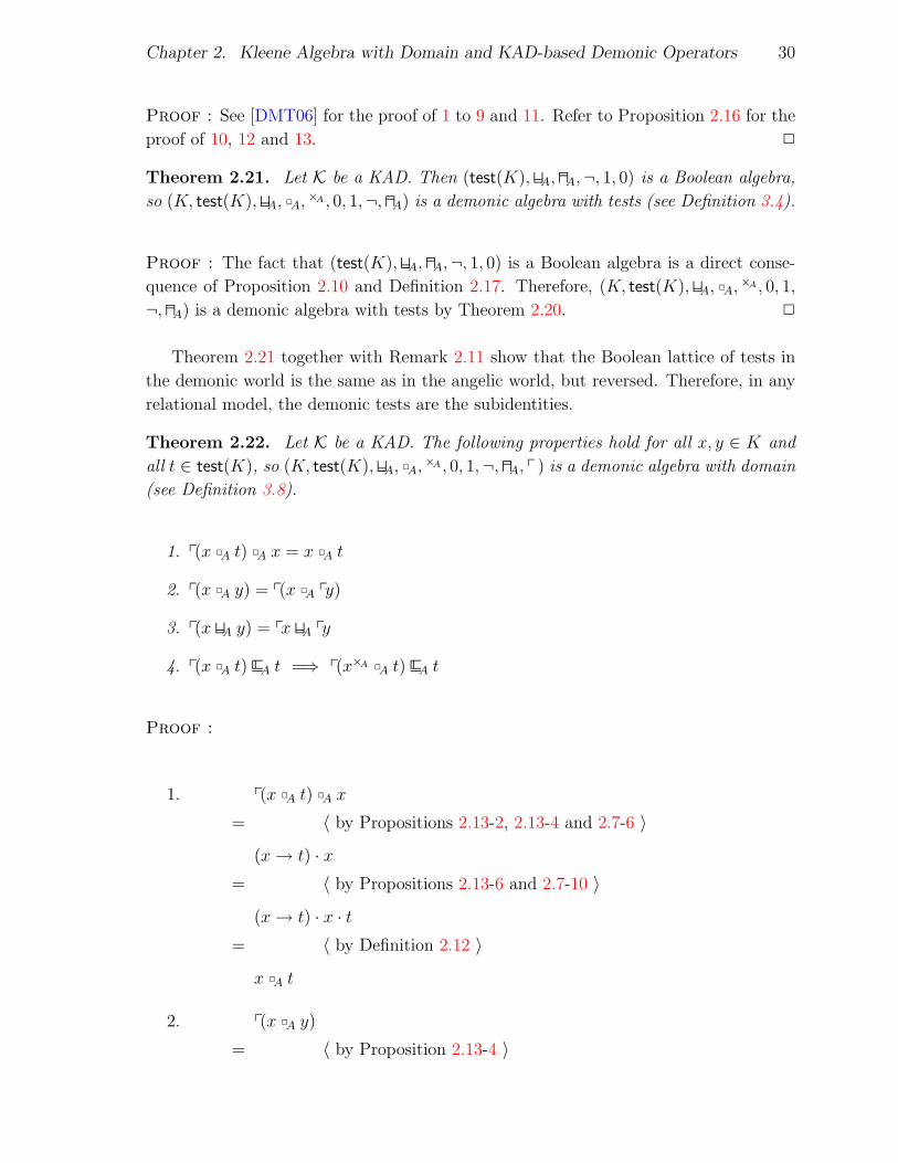
Theorem 2.21. Let K be a KAD. Then (test(K),HA,GA,¬, 1, 0) is a Boolean algebra,
so (K, test(K),HA, 2A,×A , 0, 1,¬,GA) is a demonic algebra with tests (see Definition 3.4).
Proof : The fact that (test(K),HA,GA,¬, 1, 0) is a Boolean algebra is a direct conse-
quence of Proposition 2.10 and Definition 2.17. Therefore, (K, test(K),HA, 2A,×A , 0, 1,
¬,GA) is a demonic algebra with tests by Theorem 2.20. 2
Theorem 2.21 together with Remark 2.11 show that the Boolean lattice of tests in
the demonic world is the same as in the angelic world, but reversed. Therefore, in any
relational model, the demonic tests are the subidentities.
Theorem 2.22. Let K be a KAD. The following properties hold for all x, y ∈ K and
all t ∈ test(K), so (K, test(K),HA, 2A,×A , 0, 1,¬,GA, p) is a demonic algebra with domain
(see Definition 3.8).
1. p(x 2A t) 2A x = x 2A t
2. p(x 2A y) = p(x 2A py)
3. p(x HA y) = px HA py
4. p(x 2A t) EA t =⇒ p(x×A 2A t) EA t
Proof :
1. p(x 2A t) 2A x
= 〈 by Propositions 2.13-2, 2.13-4 and 2.7-6 〉
(x→ t) · x= 〈 by Propositions 2.13-6 and 2.7-10 〉
(x→ t) · x · t= 〈 by Definition 2.12 〉
x 2A t
2. p(x 2A y)
= 〈 by Proposition 2.13-4 〉
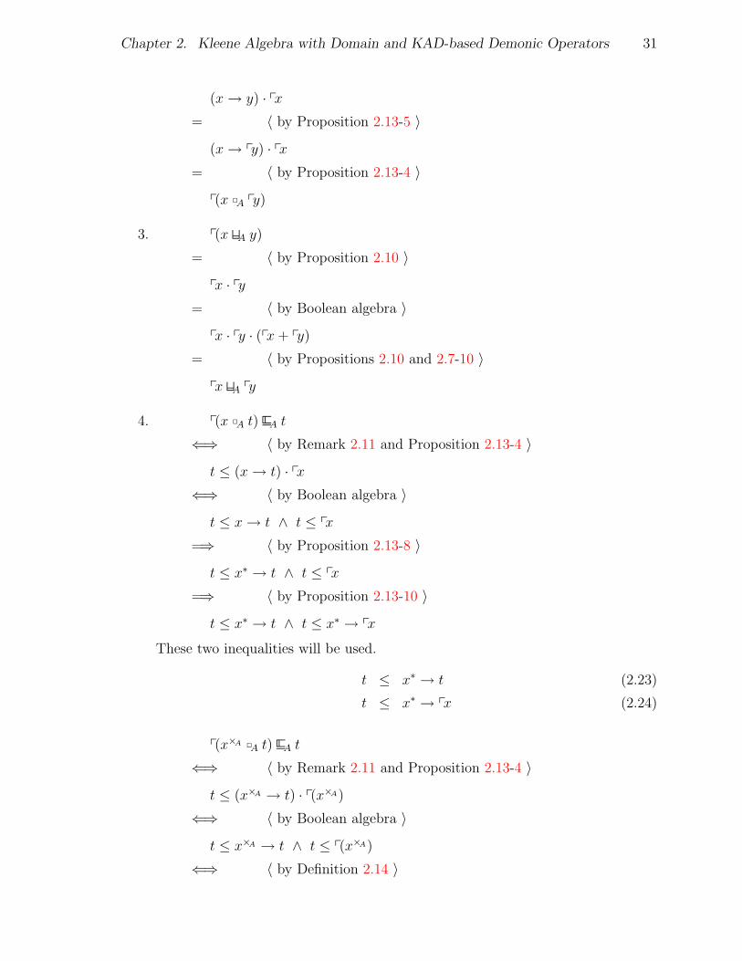
Chapter 2. Kleene Algebra with Domain and KAD-based Demonic Operators 31
(x→ y) · px= 〈 by Proposition 2.13-5 〉
(x→ py) · px= 〈 by Proposition 2.13-4 〉
p(x 2A py)
3. p(x HA y)
= 〈 by Proposition 2.10 〉
px · py= 〈 by Boolean algebra 〉
px · py · (px+ py)
= 〈 by Propositions 2.10 and 2.7-10 〉
px HA py
4. p(x 2A t) EA t
⇐⇒ 〈 by Remark 2.11 and Proposition 2.13-4 〉
t ≤ (x→ t) · px⇐⇒ 〈 by Boolean algebra 〉
t ≤ x→ t ∧ t ≤ px
=⇒ 〈 by Proposition 2.13-8 〉
t ≤ x∗ → t ∧ t ≤ px
=⇒ 〈 by Proposition 2.13-10 〉
t ≤ x∗ → t ∧ t ≤ x∗ → px
These two inequalities will be used.
t ≤ x∗ → t (2.23)
t ≤ x∗ → px (2.24)
p(x×A 2A t) EA t
⇐⇒ 〈 by Remark 2.11 and Proposition 2.13-4 〉
t ≤ (x×A → t) · p(x×A)
⇐⇒ 〈 by Boolean algebra 〉
t ≤ x×A → t ∧ t ≤ p(x×A)
⇐⇒ 〈 by Definition 2.14 〉
Chapter 2. Kleene Algebra with Domain and KAD-based Demonic Operators 32
t ≤ (x∗ 2A px) → t ∧ t ≤ p(x∗ 2A px)
⇐⇒ 〈 by Definition 2.12, Propositions 2.13-4 and 2.7-16, and (2.7) 〉
t ≤ ((x∗ → px) · x∗ · px) → t ∧ t ≤ x∗ → px
⇐⇒ 〈 by (2.24) 〉
t ≤ ((x∗ → px) · x∗ · px) → t
⇐= 〈 by Proposition 2.13-9 〉
t ≤ x∗ → t
⇐⇒ 〈 by (2.23) 〉
true
Therefore, (K, test(K),HA, 2A,×A , 0, 1,¬,GA, p ) is a demonic algebra with domain by
Theorem 2.21. 2
Theorem 2.23. Let K be a KAD. Then
x GAt y = z ⇐⇒ t 2A x = t 2A z ∧ ¬t 2A y = ¬t 2A z
for all x, y, z ∈ K and all t ∈ test(K), so (K, test(K),HA, 2A,×A , 0, 1,¬,GA, p ,GA•) is a
demonic algebra with domain and t-conditional (see Definition 3.18).
Proof :
x GAt y = z
⇐⇒ 〈 by Definition 2.18 〉
t · x+ ¬t · y = z
⇐⇒ 〈 by Proposition 2.7-3 〉
t · (t · x+ ¬t · y) = t · z ∧ ¬t · (t · x+ ¬t · y) = ¬t · z⇐⇒ 〈 by (2.8), Boolean algebra, (2.6) and (2.4) 〉
t · x = t · z ∧ ¬t · y = ¬t · z⇐⇒ 〈 by Proposition 2.13-2 〉
t 2A x = t 2A z ∧ ¬t 2A y = ¬t 2A z
Therefore, (K, test(K),HA, 2A,×A , 0, 1,¬,GA, p ,GA•) is a demonic algebra with domain
and t-conditional by Theorem 2.22. 2
Chapter 3
Axiomatisation of Demonic Algebra
with Domain and t-Conditional
In the previous chapter, we demonstrated that the demonic operators introduced in
Section 2.4 satisfy Theorems 2.20, 2.21, 2.22 and 2.23. Since we want to know how do
KADs with the demonic operators but without the usual angelic ones behave, these laws
will become axioms for a new algebraic structure called demonic algebra with domain
and t-conditional (DAD-G•). Therefore, it is easy to see that any model of KAD can
be transformed into a DAD-G• by taking the elements of the KAD and the demonic
operators defined in Section 2.4, and then forgetting the angelic operators.
We expect DAD-G• to be an algebraic foundation for the upper part of the lattice
of Figure 1.4. Also, we want to define algebraic transformations between the lower
part and the upper part of this lattice. This last goal guided our choice of laws for
the theorems of Section 2.5 and hence, our choice of axioms for Definitions 3.1, 3.4, 3.8
and 3.18.
In the presentation of the next definitions, we follow the same path as for the defini-
tion of KAD. That is, we first define demonic algebra (DA) (Section 3.1), then demonic
algebra with tests (DAT) (Section 3.2) and demonic algebra with domain (DAD) (Sec-
tion 3.3). Finally, and it is a difference between DA and KA, we need an extra operator,
so we define demonic algebra with domain and t-conditional (DAD-G•) (Section 3.4).
The reasons why we need this operator will be discussed in Section 3.4.
Chapter 3. Axiomatisation of Demonic Algebra with Domain and t-Conditional 34
3.1 Demonic Algebra
In this section, we present demonic algebra (DA), we discuss some of its axioms and we
look at a first proposition about this structure.
Like KA, DA has a sum, a composition and an iteration operator. Moreover, its
sum induces a partial order.
Definition 3.1 (Demonic algebra). A demonic algebra (DA) is a structure A =
(A,H, 2, ×,>, 1) such that the following properties are satisfied for all x, y, z ∈ A.
x H (y H z) = (x H y) H z (3.1)
x H y = y H x (3.2)
x H x = x (3.3)
> H x = > (3.4)
x2(y2z) = (x2y)2z (3.5)
>2x = x2> = > (3.6)
12x = x21 = x (3.7)
x2(y H z) = x2y H x2z (3.8)
(x H y)2z = x2z H y2z (3.9)
x× = x×2x H 1 (3.10)
There is a partial order E induced by H such that for all x, y ∈ A,
x E y ⇐⇒ x H y = y . (3.11)
The next two properties are also satisfied for all x, y, z ∈ A.
x2z H y E z =⇒ x×2y E z (3.12)
z2x H y E z =⇒ y2x× E z (3.13)
When comparing Definitions 2.1 and 3.1, one observes the obvious correspondences
+ ↔ H, · ↔ 2, ∗ ↔ ×, 0 ↔ >, 1 ↔ 1. The only difference in the axiomatisation between
KA and DA is that 0 is the left and right identity of addition in KA (+), while >is a left and right zero of addition in DA (H). However, this minor difference has a
rather important impact. While KAs and DAs are upper semilattices with + as the
join operator for KAs and H for DAs, the element 0 is the bottom of the semilattice for
KAs and > is the top of the semilattice for DAs. Indeed, by (3.4) and (3.11),
x E > (3.14)

Chapter 3. Axiomatisation of Demonic Algebra with Domain and t-Conditional 35
for all x ∈ A.
The following obvious refinements will be used in what follows.
x E x H y ∧ y E x H y (3.15)
They hold by (3.11), (3.2) and (3.3).
All operators are monotonic with respect to the refinement ordering E. That is, for
all x, y, z ∈ A,
x E y =⇒ z H x E z H y ∧ z2x E z2y ∧ x2z E y2z ∧ x× E y× .
Monotonicity of H and 2 can easily be derived from (3.11), (3.8) and (3.9). That of ×
is shown from (3.10) and (3.13) as follows:
x E y =⇒ y×2x H 1 E y×2y H 1 ⇐⇒ y×2x H 1 E y× =⇒ x× E y× .
Most of the time, this property will be used without explicit mention.
Remark 3.2. Like for the corresponding unfolding law (2.14) in KA, the following
symmetric version of (3.10),
x× = x2x× H 1 , (3.16)
is derivable from these axioms. Indeed,
x× E x2x× H 1
⇐= 〈 by (3.12) and (3.7) 〉
x2(x2x× H 1) H 1 E x2x× H 1
⇐= 〈 by monotonicity of 2 and H 〉
x2x× H 1 E x× —this is the other inequality we have to show
⇐⇒ 〈 by (3.10) 〉
x2x× H 1 E x×2x H 1
⇐= 〈 by monotonicity of H 〉
x2x× E x×2x
⇐= 〈 by (3.13) 〉
x×2x2x H x E x×2x
⇐⇒ 〈 by (3.10), (3.9) and (3.7) 〉
true .
Chapter 3. Axiomatisation of Demonic Algebra with Domain and t-Conditional 36
Also, one can show x× = µE(y :: y2x H 1) with (3.7), (3.10) and (3.13), and x× =
µE(y :: x2y H 1) with (3.7), (3.16) and (3.12).
Finally, in the presence of the other axioms, (3.12) and (3.13) are equivalent to the
following two.
x2z E z =⇒ x×2z E z (3.17)
z2x E z =⇒ z2x× E z (3.18)
The following proposition presents properties of the iteration operator ×. They
might be thought of as the demonic version of properties of the Kleene star ∗.
Proposition 3.3. Let A be a DA. The following laws hold for all x, y ∈ A.
1. 1 E x×, x×2x E x× and x2x× E x×
2. x E x×
3. x2y E y2x =⇒ x×2y E y2x×
4. y2x E x2y =⇒ y2x× E x×2y
5. x×2x× = x×
6. (x×)× = x×
7. x2(y2x)× = (x2y)×2x
8. (x H y)× = x×2(y2x×)× = (x×2y)×2x×
Proof :
1. This is direct from (3.10), (3.16) and (3.15).
2. This follows from (3.7) and Proposition 3.3-1. Indeed x = 12x E x×2x E x×.
3. Assume x2y E y2x.
x×2y E y2x×
⇐= 〈 by (3.12) 〉
x2y2x× H y E y2x×

Chapter 3. Axiomatisation of Demonic Algebra with Domain and t-Conditional 37
⇐= 〈 by the hypothesis 〉
y2x2x× H y E y2x×
⇐⇒ 〈 by (3.7), (3.8) and (3.16) 〉
true
4. Assume y2x E x2y.
y2x× E x×2y
⇐= 〈 by (3.13) 〉
x×2y2x H y E x×2y
⇐= 〈 by the hypothesis 〉
x×2x2y H y E x×2y
⇐⇒ 〈 by (3.7), (3.9) and (3.10) 〉
true
5. x×2x×
E 〈 by Proposition 3.3-1 and (3.17) 〉
x×
E 〈 by Proposition 3.3-1 〉
x×2x×
6. We first derive (x×)× E x×.
(x×)× E x×
⇐= 〈 by (3.12) and (3.7) 〉
x×2x× H 1 E x×
⇐⇒ 〈 by Propositions 3.3-1 and 3.3-5 〉
true
By Proposition 3.3-2, x× E (x×)×.
7. We first derive x2(y2x)× E (x2y)×2x.
x2(y2x)× E (x2y)×2x
⇐= 〈 by (3.13) 〉

Chapter 3. Axiomatisation of Demonic Algebra with Domain and t-Conditional 38
(x2y)×2x2y2x H x E (x2y)×2x
⇐⇒ 〈 by Proposition 3.3-1, (3.9) and (3.7) 〉
true.
The derivation of (x2y)×2x E x2(y2x)× is similar, using (3.12).
8. We first derive (x H y)× E x×2(y2x×)×.
(x H y)× E x×2(y2x×)×
⇐= 〈 by (3.12) and (3.7) 〉
(x H y)2x×2(y2x×)× H 1 E x×2(y2x×)×
⇐⇒ 〈 by Proposition 3.3-1, (3.7) and (3.9) 〉
x2x×2(y2x×)× H y2x×2(y2x×)× E x×2(y2x×)×
⇐= 〈 by Proposition 3.3-1 and (3.16) 〉
(y2x×)× E x×2(y2x×)×
⇐⇒ 〈 by Proposition 3.3-1 and (3.7) 〉
true.
And here is the derivation of x×2(y2x×)× E (x H y)×.
true
⇐⇒ 〈 by (3.15) and Proposition 3.3-2 〉
y E (x H y)× ∧ x× E (x H y)×
=⇒ 〈 by Propositions 3.3-5 and 3.3-6 〉
(y2x×)× E (x H y)× ∧ x× E (x H y)×
=⇒ 〈 by Proposition 3.3-5 〉
x×2(y2x×)× E (x H y)×
The proof of (x H y)× = (x×2y)×2x× is similar. 2
3.2 Demonic Algebra with Tests
Now comes the first extension of DA, demonic algebra with tests (DAT). This extension
has a concept of Boolean algebra of tests like the one in KAT and it also adds the G

Chapter 3. Axiomatisation of Demonic Algebra with Domain and t-Conditional 39
operator. Introducing G provides a way to express the meet of tests, as will be shown
below. In KAT, + and · are respectively the join and meet operators of the Boolean
lattice of tests. But in Section 3.3, it will turn out that for any tests s and t, sH t = s2t,
so that H and 2 both act as the join operator on tests (this is also the case for the
KAD-based definition of these operators given in Section 2.4, as can be checked).
In this section, we also discuss the implications of the definition of DAT and we
present a simple lemma related to demonic tests.
Here is how we deal with tests in a demonic world.
Definition 3.4 (Demonic algebra with tests). A demonic algebra with tests (DAT)
is a structure A = (A, test(A),H, 2, ×,>, 1,¬,G) such that {1,>} ⊆ test(A) ⊆ A,
(A,H, 2, ×,>, 1) is a DA and (test(A),H,G,¬, 1,>) is a Boolean algebra. The elements
in test(A) are called (demonic) tests. The operator G stands for the infimum of elements
in test(A) with respect to E.
Note that 1 and > are respectively the bottom and the top of the Boolean lattice
of tests. We insist that the operators G and ¬ are defined exclusively on test(A). In
the sequel, we use the letters w, x, y, z for arbitrary elements of DA and s, t, u, v for
demonic tests.
A basic property of demonic algebra with domain (DAD) (see Section 3.3) is that
s2t = sHt (see Proposition 3.14-3). Therefore, in DAD, s2¬s = sH¬s = > and ¬1 = >.
This is why we are going to say that two tests s and t are disjoint when s2t = sH t = >.
The following example presents a situation where this does not stand in DAT. It was
constructed using Mace4 [Mac].
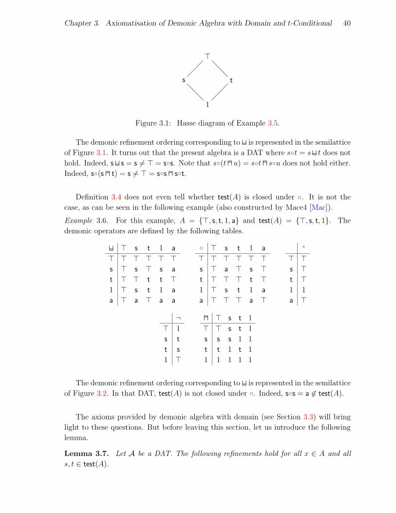
Example 3.5. For this example, A = test(A) = {>, s, t, 1}. The demonic operators are
defined by the following tables.
H > s t 1
> > > > >s > s > s
t > > t t
1 > s t 1
2 > s t 1
> > > > >s > > > s
t > > > t
1 > s t 1
×
> >s >t >1 1
¬> 1
s t
t s
1 >
G > s t 1
> > s t 1
s s s 1 1
t t 1 t 1
1 1 1 1 1
Chapter 3. Axiomatisation of Demonic Algebra with Domain and t-Conditional 40
>
����
���
>>>>
>>>>
s
????
???? t
����
����
1
Figure 3.1: Hasse diagram of Example 3.5.
The demonic refinement ordering corresponding to H is represented in the semilattice
of Figure 3.1. It turns out that the present algebra is a DAT where s2t = sH t does not
hold. Indeed, s H s = s 6= > = s2s. Note that s2(tG u) = s2tG s2u does not hold either.
Indeed, s2(s G t) = s 6= > = s2s G s2t.
Definition 3.4 does not even tell whether test(A) is closed under 2. It is not the
case, as can be seen in the following example (also constructed by Mace4 [Mac]).
Example 3.6. For this example, A = {>, s, t, 1, a} and test(A) = {>, s, t, 1}. The
demonic operators are defined by the following tables.
H > s t 1 a
> > > > > >s > s > s a
t > > t t >1 > s t 1 a
a > a > a a
2 > s t 1 a
> > > > > >s > a > s >t > > > t >1 > s t 1 a
a > > > a >
×
> >s >t >1 1
a >
¬> 1
s t
t s
1 >
G > s t 1
> > s t 1
s s s 1 1
t t 1 t 1
1 1 1 1 1
The demonic refinement ordering corresponding to H is represented in the semilattice
of Figure 3.2. In that DAT, test(A) is not closed under 2. Indeed, s2s = a 6∈ test(A).
The axioms provided by demonic algebra with domain (see Section 3.3) will bring
light to these questions. But before leaving this section, let us introduce the following
lemma.
Lemma 3.7. Let A be a DAT. The following refinements hold for all x ∈ A and all
s, t ∈ test(A).
Chapter 3. Axiomatisation of Demonic Algebra with Domain and t-Conditional 41
>
~~~~
~~~
////
////
////
//
a
s
????
???? t
����
����
1
Figure 3.2: Hasse diagram of Example 3.6.
1. x E t2x ∧ x E x2t
2. s H t E s2t
3. t2¬t = ¬t2t = >
4. 1 E s2t
5. t2x E x =⇒ > E ¬t2x
6. t E x×2t and t E t2x×
Proof :
1. true
⇐⇒ 〈 by Boolean algebra 〉
1 E t
=⇒ 〈 by (3.7) 〉
x E t2x
The proof of the second refinement is similar.
2. By Lemma 3.7-1, s E s2t and t E s2t. So s H t E s2t by (3.3).
3. >= 〈 by Boolean algebra 〉
t H ¬tE 〈 by Lemma 3.7-2 〉
t2¬tSo t2¬t = > by (3.14). The proof of the second equality is similar.
Chapter 3. Axiomatisation of Demonic Algebra with Domain and t-Conditional 42
4. By Boolean algebra, 1 E s and 1 E t. So 1 E s2t by (3.7).
5. t2x E x
=⇒ 〈 〉
¬t2t2x E ¬t2x
⇐⇒ 〈 by Lemma 3.7-3 〉
>2x E ¬t2x
⇐⇒ 〈 by (3.6) 〉
> E ¬t2x
6. By Proposition 3.3-1, t = 12t E x×2t and t = t21 E t2x×. 2
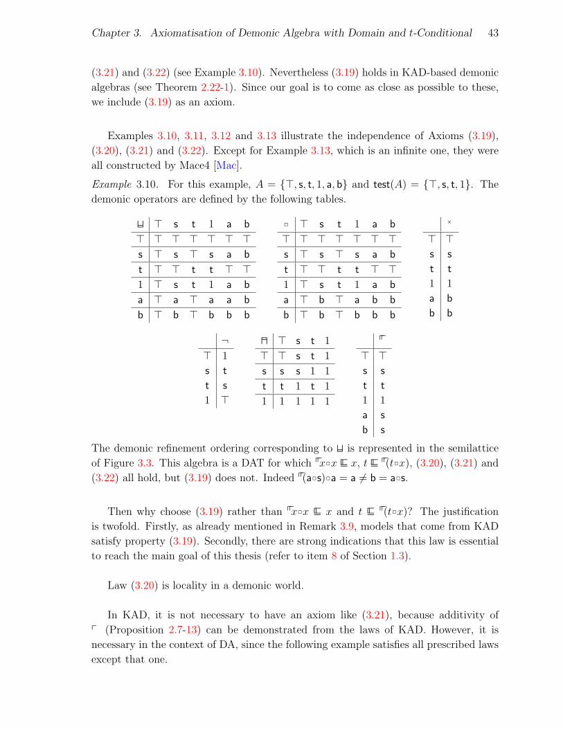
3.3 Demonic Algebra with Domain
Still following KAD’s footsteps, the next extension consists in adding a domain operator
to DAT to obtain the demonic algebra with domain (DAD). In this section, we also
demonstrate that axioms of DAD are independent, we present an important proposition
about the domain operator (Proposition 3.14) and we demonstrate a technical lemma
that is going to simplify many derivations in subsequent chapters.
In the demonic world, we denote the domain operator by the symbol pp.
Definition 3.8 (Demonic algebra with domain). A demonic algebra with domain
(DAD) is a structure A = (A, test(A),H, 2, ×,>, 1,¬,G, pp), where (A, test(A),H, 2, ×,>,1,¬,G) is a DAT, and the domain operator pp : A → test(A) satisfies the following
properties for all x, y ∈ A and all t ∈ test(A).
pp(x2t)2x = x2t (3.19)
pp(x2y) = pp(x2ppy) (3.20)
pp(x H y) = ppx H ppy (3.21)
pp(x2t) E t =⇒ pp(x×2t) E t (3.22)
Remark 3.9. As noted above, the axiomatisation of DA (respectively DAT) is very sim-
ilar to that of KA (respectively KAT), so one might expect the resemblance to continue
between DAD and KAD. In particular, looking at the angelic version of Definition 3.8,
namely Definition 2.4, one might expect to find axioms like ppx2x E x and t E pp(t2x).
These two properties can be derived from the chosen axioms (see Propositions 3.14-
7 and 3.14-10) but (3.19) cannot be derived from them, even when assuming (3.20),
Chapter 3. Axiomatisation of Demonic Algebra with Domain and t-Conditional 43
(3.21) and (3.22) (see Example 3.10). Nevertheless (3.19) holds in KAD-based demonic
algebras (see Theorem 2.22-1). Since our goal is to come as close as possible to these,
we include (3.19) as an axiom.
Examples 3.10, 3.11, 3.12 and 3.13 illustrate the independence of Axioms (3.19),
(3.20), (3.21) and (3.22). Except for Example 3.13, which is an infinite one, they were
all constructed by Mace4 [Mac].
Example 3.10. For this example, A = {>, s, t, 1, a, b} and test(A) = {>, s, t, 1}. The
demonic operators are defined by the following tables.
H > s t 1 a b
> > > > > > >s > s > s a b
t > > t t > >1 > s t 1 a b
a > a > a a b
b > b > b b b
2 > s t 1 a b
> > > > > > >s > s > s a b
t > > t t > >1 > s t 1 a b
a > b > a b b
b > b > b b b
×
> >s s
t t
1 1
a b
b b
¬> 1
s t
t s
1 >
G > s t 1
> > s t 1
s s s 1 1
t t 1 t 1
1 1 1 1 1
pp
> >s s
t t
1 1
a s
b s
The demonic refinement ordering corresponding to H is represented in the semilattice
of Figure 3.3. This algebra is a DAT for which ppx2x E x, t E pp(t2x), (3.20), (3.21) and
(3.22) all hold, but (3.19) does not. Indeed pp(a2s)2a = a 6= b = a2s.
Then why choose (3.19) rather than ppx2x E x and t E pp(t2x)? The justification
is twofold. Firstly, as already mentioned in Remark 3.9, models that come from KAD
satisfy property (3.19). Secondly, there are strong indications that this law is essential
to reach the main goal of this thesis (refer to item 8 of Section 1.3).
Law (3.20) is locality in a demonic world.
In KAD, it is not necessary to have an axiom like (3.21), because additivity of
p (Proposition 2.7-13) can be demonstrated from the laws of KAD. However, it is
necessary in the context of DA, since the following example satisfies all prescribed laws
except that one.

Chapter 3. Axiomatisation of Demonic Algebra with Domain and t-Conditional 44
>
����
���
****
****
****
****
****
*
b
a
s
????
???? t
����
����
1
Figure 3.3: Hasse diagram of Example 3.10.
>
����
���
>>>>
>>>>
s
????
????
a t
����
����
1
Figure 3.4: Hasse diagram of Example 3.11.
Example 3.11. For this example, A = {>, s, t, 1, a} and test(A) = {>, s, t, 1}. The
demonic operators are defined by the following tables.
H > s t 1 a
> > > > > >s > s > s >t > > t t >1 > s t 1 >a > > > > a
2 > s t 1 a
> > > > > >s > s > s a
t > > t t >1 > s t 1 a
a > > > a >
×
> >s s
t t
1 1
a >
¬> 1
s t
t s
1 >
G > s t 1
> > s t 1
s s s 1 1
t t 1 t 1
1 1 1 1 1
pp
> >s s
t t
1 1
a s
The demonic refinement ordering corresponding to H is represented in the semilattice
of Figure 3.4. This algebra is a DAT and, in addition, (3.19), (3.20) and (3.22) are
satisfied, but (3.21) is not. Indeed pp(1 H a) = > 6= s = pp1 H ppa.
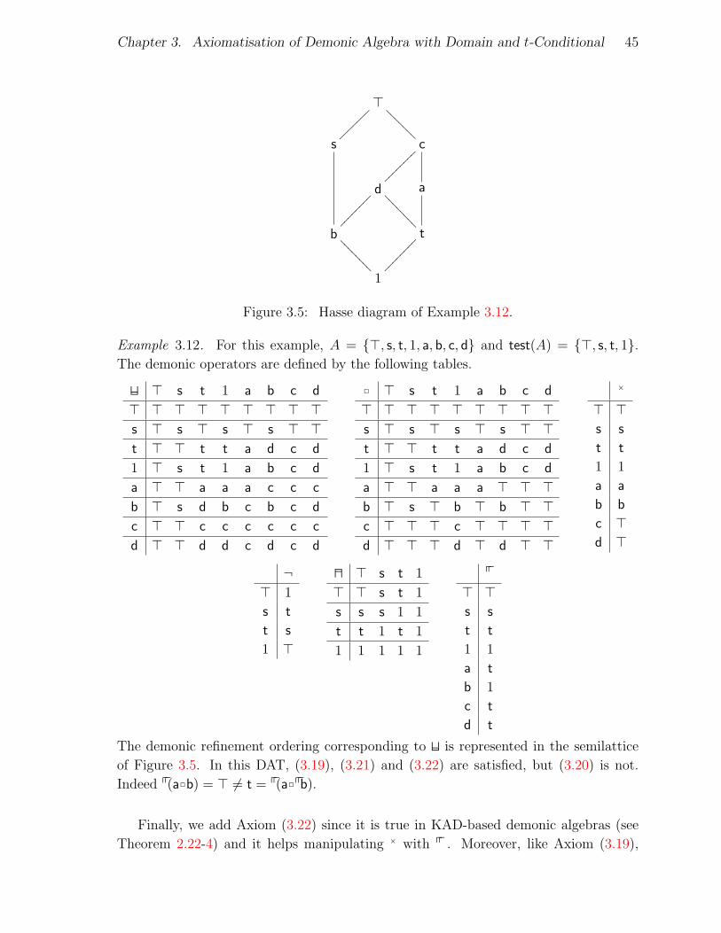
Chapter 3. Axiomatisation of Demonic Algebra with Domain and t-Conditional 45
>
~~~~
~~~
@@@@
@@@
s c
~~~~
~~~~
d
����
����
>>>>
>>>>
a
b
????
????
t
����
����
1
Figure 3.5: Hasse diagram of Example 3.12.
Example 3.12. For this example, A = {>, s, t, 1, a, b, c, d} and test(A) = {>, s, t, 1}.The demonic operators are defined by the following tables.
H > s t 1 a b c d
> > > > > > > > >s > s > s > s > >t > > t t a d c d
1 > s t 1 a b c d
a > > a a a c c c
b > s d b c b c d
c > > c c c c c c
d > > d d c d c d
2 > s t 1 a b c d
> > > > > > > > >s > s > s > s > >t > > t t a d c d
1 > s t 1 a b c d
a > > a a a > > >b > s > b > b > >c > > > c > > > >d > > > d > d > >
×
> >s s
t t
1 1
a a
b b
c >d >
¬> 1
s t
t s
1 >
G > s t 1
> > s t 1
s s s 1 1
t t 1 t 1
1 1 1 1 1
pp
> >s s
t t
1 1
a t
b 1
c t
d t
The demonic refinement ordering corresponding to H is represented in the semilattice
of Figure 3.5. In this DAT, (3.19), (3.21) and (3.22) are satisfied, but (3.20) is not.
Indeed pp(a2b) = > 6= t = pp(a2ppb).
Finally, we add Axiom (3.22) since it is true in KAD-based demonic algebras (see
Theorem 2.22-4) and it helps manipulating × with pp . Moreover, like Axiom (3.19),

Chapter 3. Axiomatisation of Demonic Algebra with Domain and t-Conditional 46
there are strong indications that this law is essential to reach the main goal of this
thesis.
Examples 3.10, 3.11 and 3.12 show that Axioms (3.19), (3.20) and (3.21) are inde-
pendent from each other and also from (3.22). The following example completes the
proof of independence of (3.19), (3.20), (3.21) and (3.22).
Example 3.13. For this example, A = {E : ℘(N) | E is finite} and test(A) = {{}, {0}}.The demonic operators are as follows.
H : A× A −→ A
(E,F ) 7→{E ∪ F if E 6= {} and F 6= {}{} if E = {} or F = {}
2 : A× A −→ A
(E,F ) 7→ {x : N | (∃ e : E, f : F | x = e+ f)}
× : A −→ A
E 7→{{0} if E = {0}{} if E 6= {0}
pp : A −→ test(A)
E 7→{{0} if E 6= {}{} if E = {}
Hence {} is the top of the upper semilattice (A,E) and {0} is neutral for demonic
composition. Since the only tests are {0} and {}, the operators ¬ and G are trivially
defined. In this DAT, (3.19), (3.20) and (3.21) are satisfied, but (3.22) is not. Indeed,
pp({1}2{0}) E {0} ⇐⇒ true 6=⇒ false ⇐⇒ pp({1}×2{0}) E {0} .
By Proposition 3.14-7 below, ppx is a left preserver of x. By Proposition 3.14-14, it
is the greatest left preserver. Similarly, by Proposition 3.14-17, ¬ppx is a left annihilator
of x. By Proposition 3.14-16, it is the least left annihilator (since Proposition 3.14-16
can be rewritten as ¬ppx E t ⇐⇒ > E t2x). Hence, on the left of the equivalence of
Proposition 3.14-13, t acts as a left preserver of x and on the right, ¬t acts as a left
annihilator.
The axioms of DAD impose important restrictions on demonic tests. It turns out
that these restrictions are actually useful properties and they are presented in the
following proposition together with properties of pp.

Chapter 3. Axiomatisation of Demonic Algebra with Domain and t-Conditional 47
Proposition 3.14. Let A be a DAD. The following laws hold for all x, y ∈ A and all
s, t, u ∈ test(A).
1. ppt = t
2. t2t = t
3. s H t = s2t and hence test(A) is closed under 2
4. s2(t G u) = s2t G s2u and (s G t)2u = s2u G t2u
5. s2t = t2s
6. x E t2y ⇐⇒ t2x E t2y
7. ppx2x = x
8. x E y =⇒ ppx E ppy
9. pp(t2x) = t2ppx
10. t E pp(t2x)
11. x H y = ppx2ppy2(x H y)
12. pp(x2s)2pp(x2t) = pp(x2s2t)
13. t2x E x ⇐⇒ > E ¬t2x
14. t E ppx ⇐⇒ t2x E x
15. ppx = maxE{t : test(A) | t2x = x}
16. t E ppx ⇐⇒ > E ¬t2x
17. ¬ppx2x = >
18. ppx E pp(x2y)
19. ppx = > ⇐⇒ x = >
20. t2(x H y) = t2x H y = x H t2y
21. ppx2ppy = > =⇒ ppx2y = ppy2x
22. ppx = 1 =⇒ pp(x×) = 1
Proof :

Chapter 3. Axiomatisation of Demonic Algebra with Domain and t-Conditional 48
1. This is direct from (3.19) with x := 1 and (3.7).
2. This is direct from (3.19) with x, t := t, 1, (3.7) and Proposition 3.14-1.
3. s2t
E 〈 by (3.15) 〉
(s H t)2(s H t)
= 〈 by Proposition 3.14-2 〉
s H t
E 〈 by Lemma 3.7-2 〉
s2t
4. This follows from Proposition 3.14-3 and Boolean algebra.
5. This follows from Proposition 3.14-3 and Boolean algebra.
6. x E t2y
=⇒ 〈 〉
t2x E t2t2y
⇐⇒ 〈 by Proposition 3.14-2 〉
t2x E t2y
=⇒ 〈 by Lemma 3.7-1 and transitivity of E 〉
x E t2y
7. This is direct from (3.19) with t := 1 and (3.7).
8. x E y
⇐⇒ 〈 by (3.11) 〉
x H y = y
=⇒ 〈 by Leibniz and (3.21) 〉
ppx H ppy = ppy
⇐⇒ 〈 by (3.11) 〉
ppx E ppy
9. t2ppx
= 〈 by Propositions 3.14-3 and 3.14-1 〉
pp(t2ppx)
Chapter 3. Axiomatisation of Demonic Algebra with Domain and t-Conditional 49
= 〈 by (3.20) 〉
pp(t2x)
10. By Lemma 3.7-1 and Proposition 3.14-9, t E t2ppx = pp(t2x).
11. x H y
= 〈 by Proposition 3.14-7 〉
pp(x H y)2(x H y)
= 〈 by (3.21) 〉
(ppx H ppy)2(x H y)
= 〈 by Proposition 3.14-3 〉
ppx2ppy2(x H y)
12. pp(x2s)2pp(x2t)
= 〈 by Proposition 3.14-3 〉
pp(x2s) H pp(x2t)
= 〈 by ( 3.21) 〉
pp((x2s) H (x2t))
= 〈 by (3.8) 〉
pp(x2(s H t))
= 〈 by Proposition 3.14-3 〉
pp(x2s2t)
13. t2x E x
=⇒ 〈 by Lemma 3.7-5 〉
> E ¬t2x
=⇒ 〈 by Proposition 3.14-8 〉
pp> E pp(¬t2x)
⇐⇒ 〈 by Propositions 3.14-1 and 3.14-9 〉
> E ¬t2ppx
=⇒ 〈 by Boolean algebra 〉
t2ppx E t2ppx G ¬t2ppx
⇐⇒ 〈 by Proposition 3.14-4, Boolean algebra and (3.7) 〉
t2ppx E ppx

Chapter 3. Axiomatisation of Demonic Algebra with Domain and t-Conditional 50
=⇒ 〈 by Proposition 3.14-7 〉
t2x E x
14. [=⇒] By assumption, monotonicity of 2 and Proposition 3.14-7, t2x E ppx2x = x.
[⇐=]
t2x E x
=⇒ 〈 by Proposition 3.14-8 〉
pp(t2x) E ppx
=⇒ 〈 by Proposition 3.14-10 〉
t E ppx
15. This is direct from Proposition 3.14-14.
16. This is direct from Propositions 3.14-14 and 3.14-13.
17. This law follows directly from Proposition 3.14-16 and (3.14).
18. Since ppx2(x2y) = (ppx2x)2y = x2y, the result follows from Proposition 3.14-14.
19. ppx = >⇐⇒ 〈 by (3.14) 〉
> E ppx
⇐⇒ 〈 by Proposition 3.14-14 〉
>2x E x
⇐⇒ 〈 by (3.6) 〉
> E x
⇐⇒ 〈 by (3.14) 〉
x = >
20. t2x H y
= 〈 by Proposition 3.14-11 〉
pp(t2x)2ppy2(t2x H y)
= 〈 by Proposition 3.14-9 〉
t2ppx2ppy2(t2x H y)
= 〈 by Propositions 3.14-5 and 3.14-2, and (3.8) 〉

Chapter 3. Axiomatisation of Demonic Algebra with Domain and t-Conditional 51
t2ppx2t2ppy2(t2x H t2y)
= 〈 by Proposition 3.14-9 〉
pp(t2x)2pp(t2y)2(t2x H t2y)
= 〈 by Proposition 3.14-11 and (3.8) 〉
t2(x H y)
The derivation for the second equality is similar.
21. ppx2ppy = >⇐⇒ 〈 by Propositions 3.14-19 and 3.14-9, and Boolean algebra 〉
ppx2y = > ∧ ppy2x = >=⇒ 〈 〉
ppx2y = ppy2x
22. ppx = 1
⇐⇒ 〈 by (3.7) and Boolean algebra 〉
pp(x21) E 1
=⇒ 〈 by (3.22) 〉
pp(x×21) E 1
⇐⇒ 〈 by (3.7) and Boolean algebra 〉
pp(x×) = 1
2
All the above laws except 12 are identical to laws of p , after compensating for the
reverse ordering of the Boolean lattice (on tests, E corresponds to ≥).
Although Proposition 3.14-1 is a quite basic property, its proof uses (3.19). Further-
more, Proposition 3.14-1 and (3.19) are used in the proof of Propositions 3.14-2, 3.14-3,
3.14-4, 3.14-5, 3.14-6 and 3.14-7. Since (3.19) is not as natural as the others, it would
be interesting to find an argument that only involves (3.20) and (3.21). It turns out
that it is not possible. Indeed, see Example 3.15 (also constructed by Mace4 [Mac]).
Example 3.15. For this example, A = test(A) = {>, s, t, 1}. The demonic operators

Chapter 3. Axiomatisation of Demonic Algebra with Domain and t-Conditional 52
>
����
���
>>>>
>>>>
s
????
???? t
����
����
1
Figure 3.6: Hasse diagram of Example 3.15.
are defined by the following tables.
H > s t 1
> > > > >s > s > s
t > > t t
1 > s t 1
2 > s t 1
> > > > >s > > > s
t > > > t
1 > s t 1
×
> >s >t >1 1
¬> 1
s t
t s
1 >
G > s t 1
> > s t 1
s s s 1 1
t t 1 t 1
1 1 1 1 1
pp
> >s >t >1 >
The demonic refinement ordering corresponding to H is represented in the semilattice
of Figure 3.6. This algebra is a DAT and, in addition, (3.20), (3.21) and (3.22) are
satisfied, but (3.19) and ppt = t are not. Indeed pp(s21)2s = > 6= s = s21 and pp1 = > 6= 1.
Note that Propositions 3.14-2, 3.14-3, 3.14-4, 3.14-6 and 3.14-7 are not satisfied neither.
For those who are wondering, the major difference between Example 3.10 and Ex-
ample 3.15 is that ppx2x E x is satisfied in the former and not in the latter.
The following derivation closes the discussion about the choice of axioms for DAD.
Suppose ppx2x E x and t E pp(t2x) for all x ∈ A and all t ∈ test(A). Then, by Lemma 3.7-
1, one has ppt2t E t E ppt2t, so that ppt2t = t. Therefore,
t
E 〈 by the hypothesis with x, t := 1, t 〉
ppt
E 〈 by Lemma 3.7-1 〉

Chapter 3. Axiomatisation of Demonic Algebra with Domain and t-Conditional 53
ppt2t
= 〈 derived above from the hypothesis 〉
t ,
so ppt = t.
In conclusion,
ppx2x E x ∧ t E pp(t2x) ∧ (3.20) ∧ (3.21) 6=⇒ (3.19) ,
(3.19) ∧ (3.20) ∧ (3.21) =⇒ ppx2x E x ∧ t E pp(t2x) ,
(3.20) ∧ (3.21) 6=⇒ ppt = t ,
ppx2x E x ∧ t E pp(t2x) ∧ (3.20) ∧ (3.21) =⇒ ppt = t .
Remark 3.16. Since in any DADA, s2t = sHt for all s, t ∈ test(A) (see Proposition 3.14-
3), the Boolean algebra of demonic tests test(A) may be viewed as (test(A),H,G,¬, 1,>)
or as (test(A), 2,G,¬, 1,>). Therefore, each time we use a law from Boolean algebra,
whether it is written with H or with 2, we will invoke “Boolean algebra”.
We finish this section with a lemma that will mostly be used in Sections 4.4 and 4.5.
It is presented here because it is a natural continuation of Proposition 3.14.
Lemma 3.17. In any DAD A, the domain operator satisfies the following properties
for all x ∈ A and all s, t ∈ test(A).
1. ppx2pp(x2t) = pp(x2t)
2. ¬ppx2pp(x2t) = >
3. ¬ppx2¬pp(x2t) = ¬ppx
4. pp(x2t)2pp(x2¬t) = >
5. pp(x2t)2¬pp(x2¬t) = pp(x2t) and hence ¬pp(x2¬t) E pp(x2t)
6. pp(x2(s G t)) E pp(x2s) and pp(x2(s G t)) E pp(x2t)
Proof :
1. It follows from Propositions 3.14-9 and 3.14-7.
Chapter 3. Axiomatisation of Demonic Algebra with Domain and t-Conditional 54
2. It follows from Propositions 3.14-9, 3.14-17, and 3.14-1, and (3.6).
3. true
⇐⇒ 〈 by Proposition 3.14-18 〉
ppx E pp(x2t)
⇐⇒ 〈 by Boolean algebra and Proposition 3.14-3 〉
¬ppx2¬pp(x2t) = ¬ppx
4. It follows from Propositions 3.14-12, and 3.14-1, and (3.6).
5. true
⇐⇒ 〈 by Lemma 3.17-4 〉
pp(x2t)2pp(x2¬t) = >⇐⇒ 〈 by Proposition 3.14-3 and Boolean algebra 〉
¬pp(x2¬t) E pp(x2t)
⇐⇒ 〈 by Boolean algebra and Proposition 3.14-3 〉
pp(x2t)2¬pp(x2¬t) = pp(x2t)
6. It follows from Boolean algebra and Proposition 3.14-8. 2
3.4 Demonic Algebra with Domain and t-Conditio-
nal
At this point, we have defined DA, which is an algebraic foundation for the upper part
of the lattice of Figure 1.4 and we have extended it to DAT and then to DAD in such
a way that we followed the same path as for the definition of KAD. In this section, we
define another operator, the t-conditional operator G•. We also demonstrate that the
definition of the G• operator is independent from the definition of DAD.
There are two important reasons why we need this extra operator. Now that we
have an algebraic foundation for both the lower and the upper part of the lattice of
Figure 1.4, we are looking for connections between those parts of the lattice. The
upward link from KAD to DAD is well defined thanks to Theorems 2.20, 2.21 and 2.22.
The strategy to define a downward link from DAD to KAD could be inspired by the
one for the upward link: define angelic operators from DAD and demonstrate that the
elements of DAD together with these angelic operators constitute a KAD. But it is
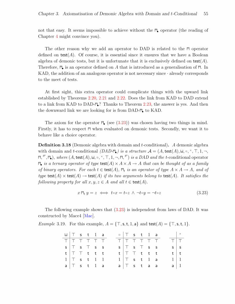
Chapter 3. Axiomatisation of Demonic Algebra with Domain and t-Conditional 55
not that easy. It seems impossible to achieve without the G• operator (the reading of
Chapter 4 might convince you).
The other reason why we add an operator to DAD is related to the G operator
defined on test(A). Of course, it is essential since it ensures that we have a Boolean
algebra of demonic tests, but it is unfortunate that it is exclusively defined on test(A).
Therefore, G• is an operator defined on A that is introduced as a generalisation of G. In
KAD, the addition of an analogous operator is not necessary since · already corresponds
to the meet of tests.
At first sight, this extra operator could complicate things with the upward link
established by Theorems 2.20, 2.21 and 2.22. Does the link from KAD to DAD extend
to a link from KAD to DAD-G•? Thanks to Theorem 2.23, the answer is yes. And then
the downward link we are looking for is from DAD-G• to KAD.
The axiom for the operator G• (see (3.23)) was chosen having two things in mind.
Firstly, it has to respect G when evaluated on demonic tests. Secondly, we want it to
behave like a choice operator.
Definition 3.18 (Demonic algebra with domain and t-conditional). A demonic algebra
with domain and t-conditional (DAD-G•) is a structure A = (A, test(A),H, 2, ×,>, 1,¬,G, pp,G•), where (A, test(A),H, 2, ×,>, 1,¬,G, pp) is a DAD and the t-conditional operator
G• is a ternary operator of type test(A)×A×A→ A that can be thought of as a family
of binary operators. For each t ∈ test(A), Gt is an operator of type A×A→ A, and of
type test(A)× test(A) → test(A) if its two arguments belong to test(A). It satisfies the
following property for all x, y, z ∈ A and all t ∈ test(A).
x Gt y = z ⇐⇒ t2x = t2z ∧ ¬t2y = ¬t2z (3.23)
The following example shows that (3.23) is independent from laws of DAD. It was
constructed by Mace4 [Mac].
Example 3.19. For this example, A = {>, s, t, 1, a} and test(A) = {>, s, t, 1}.
H > s t 1 a
> > > > > >s > s > s s
t > > t t t
1 > s t 1 1
a > s t 1 a
2 > s t 1 a
> > > > > >s > s > s s
t > > t t t
1 > s t 1 a
a > s t a a
×
> >s s
t t
1 1
a 1
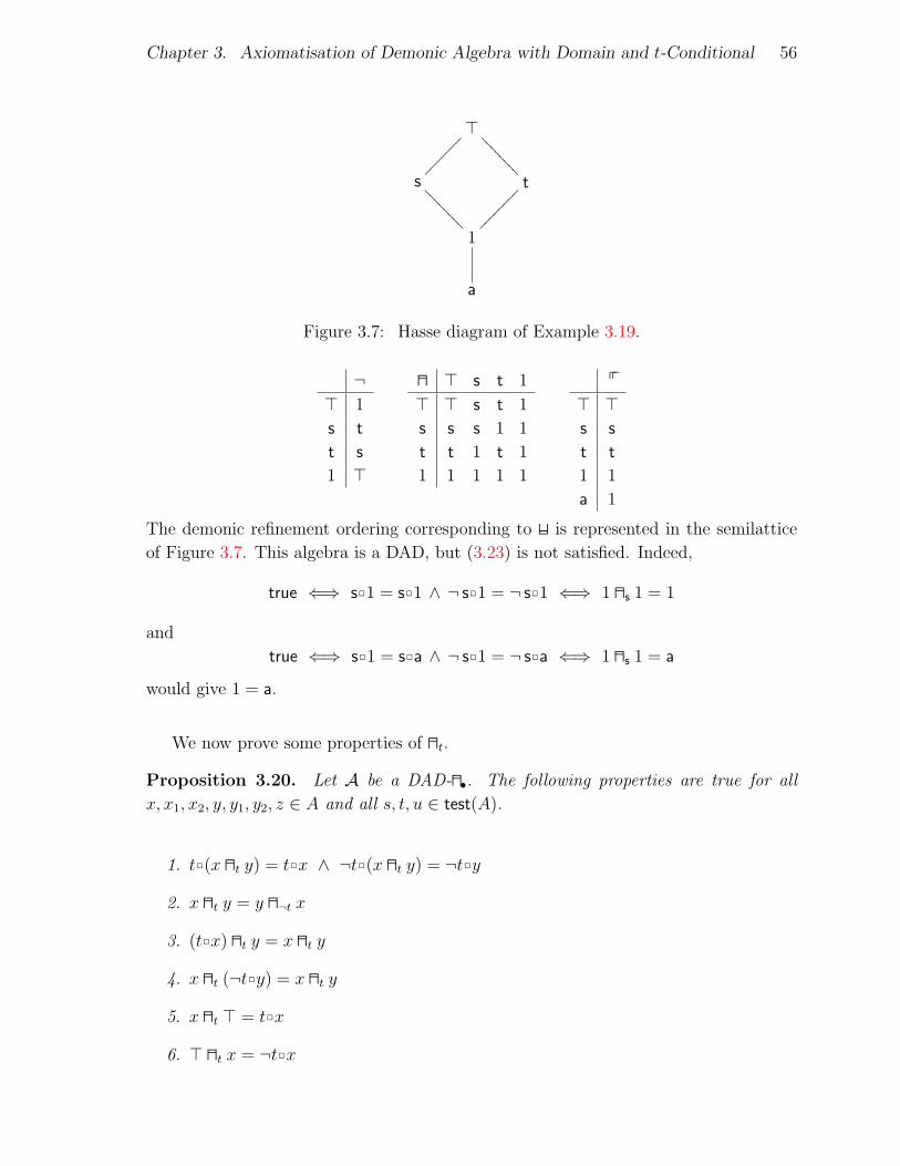
Chapter 3. Axiomatisation of Demonic Algebra with Domain and t-Conditional 56
>
����
���
>>>>
>>>>
s
????
???? t
����
����
1
a
Figure 3.7: Hasse diagram of Example 3.19.
¬> 1
s t
t s
1 >
G > s t 1
> > s t 1
s s s 1 1
t t 1 t 1
1 1 1 1 1
pp
> >s s
t t
1 1
a 1
The demonic refinement ordering corresponding to H is represented in the semilattice
of Figure 3.7. This algebra is a DAD, but (3.23) is not satisfied. Indeed,
true ⇐⇒ s21 = s21 ∧ ¬ s21 = ¬ s21 ⇐⇒ 1 Gs 1 = 1
and
true ⇐⇒ s21 = s2a ∧ ¬ s21 = ¬ s2a ⇐⇒ 1 Gs 1 = a
would give 1 = a.
We now prove some properties of Gt.
Proposition 3.20. Let A be a DAD-G•. The following properties are true for all
x, x1, x2, y, y1, y2, z ∈ A and all s, t, u ∈ test(A).
1. t2(x Gt y) = t2x ∧ ¬t2(x Gt y) = ¬t2y
2. x Gt y = y G¬t x
3. (t2x) Gt y = x Gt y
4. x Gt (¬t2y) = x Gt y
5. x Gt > = t2x
6. > Gt x = ¬t2x

Chapter 3. Axiomatisation of Demonic Algebra with Domain and t-Conditional 57
7. (x Gt y)2z = x2z Gt y2z
8. s2(x Gt y) = s2x Gt s2y
9. x Gt (y H z) = (x Gt y) H (x Gt z)
10. x H (y Gt z) = (x H y) Gt (x H z)
11. 1 Gs t = s G t
12. s Gt u = t2s G ¬t2u
13. x Gt x = x
14. x E y =⇒ x Gt z E y Gt z
15. x E y =⇒ z Gt x E z Gt y
16. x E y ⇐⇒ t2x E t2y ∧ ¬t2x E ¬t2y
17. x = y ⇐⇒ t2x = t2y ∧ ¬t2x = ¬t2y
18. x E y Gt z ⇐⇒ x E t2y ∧ x E ¬t2z
19. (x1 Gs y1) Gt (x2 Gs y2) = (x1 Gt x2) Gs (y1 Gt y2)
20. pp(x Gt y) = ppx Gt ppy
21. The demonic meet of t2x and ¬t2y with respect to E exists and is equal to xGt y.
Proof :
1. true
⇐⇒ 〈 〉
x Gt y = x Gt y
⇐⇒ 〈 by (3.23) 〉
t2(x Gt y) = t2x ∧ ¬t2(x Gt y) = ¬t2y
2. x Gt y = y G¬t x
⇐⇒ 〈 by (3.23) 〉
t2x = t2(y G¬t x) ∧ ¬t2y = ¬t2(y G¬t x)
⇐⇒ 〈 by Boolean algebra 〉

Chapter 3. Axiomatisation of Demonic Algebra with Domain and t-Conditional 58
t2x = ¬¬t2(y G¬t x) ∧ ¬t2y = ¬t2(y G¬t x)
⇐⇒ 〈 by Proposition 3.20-1 〉
t2x = ¬¬t2x ∧ ¬t2y = ¬t2y
⇐⇒ 〈 by Boolean algebra 〉
true
3. (t2x) Gt y = x Gt y
⇐⇒ 〈 by (3.23) 〉
t2t2x = t2(x Gt y) ∧ ¬t2y = ¬t2(x Gt y)
⇐⇒ 〈 by Proposition 3.20-1 〉
t2t2x = t2x ∧ ¬t2y = ¬t2y
⇐⇒ 〈 by Boolean algebra 〉
true
4. x Gt (¬t2y)
= 〈 by Proposition 3.20-2 〉
(¬t2y) G¬t x
= 〈 by Proposition 3.20-3 〉
y G¬t x
= 〈 by Proposition 3.20-2 〉
x Gt y
5. x Gt > = t2x
⇐⇒ 〈 by (3.23) 〉
t2x = t2t2x ∧ ¬t2> = ¬t2t2x
⇐⇒ 〈 by Boolean algebra 〉
t2x = t2x ∧ > = >2x
⇐⇒ 〈 by (3.6) 〉
true
6. > Gt x
= 〈 by Proposition 3.20-2 〉
x G¬t >= 〈 by Proposition 3.20-5 〉

Chapter 3. Axiomatisation of Demonic Algebra with Domain and t-Conditional 59
¬t2x
7. x2z Gt y2z = (x Gt y)2z
⇐⇒ 〈 by (3.23) 〉
t2x2z = t2(x Gt y)2z ∧ ¬t2y2z = ¬t2(x Gt y)2z
⇐⇒ 〈 by Proposition 3.20-1 〉
true
8. s2x Gt s2y = s2(x Gt y)
⇐⇒ 〈 by (3.23) 〉
t2s2x = t2s2(x Gt y) ∧ ¬t2s2y = ¬t2s2(x Gt y)
⇐⇒ 〈 by Boolean algebra 〉
s2t2x = s2t2(x Gt y) ∧ s2¬t2y = s2¬t2(x Gt y)
⇐⇒ 〈 by Proposition 3.20-1 〉
true
9. x Gt (y H z) = (x Gt y) H (x Gt z)
⇐⇒ 〈 by (3.23) 〉
t2x = t2((x Gt y) H (x Gt z)) ∧ ¬t2(y H z) = ¬t2((x Gt y) H (x Gt z))
⇐⇒ 〈 by (3.8) 〉
t2x = t2(x Gt y) H t2(x Gt z) ∧ ¬t2y H ¬t2z = ¬t2(x Gt y) H ¬t2(x Gt z)
⇐⇒ 〈 by Proposition 3.20-1 and (3.3) 〉
true
10. (x H y) Gt (x H z) = x H (y Gt z)
⇐⇒ 〈 by (3.23) 〉
t2(x H y) = t2(x H (y Gt z)) ∧ ¬t2(x H z) = ¬t2(x H (y Gt z))
⇐⇒ 〈 by (3.8) 〉
t2x H t2y = t2x H t2(y Gt z) ∧ ¬t2x H ¬t2z = ¬t2x H ¬t2(y Gt z)
⇐⇒ 〈 by Proposition 3.20-1 〉
true
11. 1 Gs t = s G t
⇐⇒ 〈 by (3.23) and Boolean algebra 〉

Chapter 3. Axiomatisation of Demonic Algebra with Domain and t-Conditional 60
s = s2(s G t) ∧ ¬s2t = ¬s2(s G t)
⇐⇒ 〈 by Boolean algebra 〉
true
12. s Gt u = t2s G ¬t2u
⇐⇒ 〈 by (3.23) 〉
t2s = t2(t2s G ¬t2u) ∧ ¬t2u = ¬t2(t2s G ¬t2u)
⇐⇒ 〈 by Boolean algebra 〉
true
13. This is direct from (3.23).
14. x E y
⇐⇒ 〈 by (3.11) 〉
x H y = y
=⇒ 〈 by Leibniz 〉
(x H y) Gt z = y Gt z
⇐⇒ 〈 by Proposition 3.20-2 〉
z G¬t (x H y) = y Gt z
⇐⇒ 〈 by Proposition 3.20-9 〉
(z G¬t x) H (z G¬t y) = y Gt z
⇐⇒ 〈 by Proposition 3.20-2 〉
(x Gt z) H (y Gt z) = y Gt z
⇐⇒ 〈 by (3.11) 〉
x Gt z E y Gt z
15. x E y
=⇒ 〈 by Proposition 3.20-14 〉
x G¬t z E y G¬t z
⇐⇒ 〈 by Proposition 3.20-2 〉
z Gt x E z Gt y
16. x E y
=⇒ 〈 〉

Chapter 3. Axiomatisation of Demonic Algebra with Domain and t-Conditional 61
t2x E t2y ∧ ¬t2x E ¬t2y
=⇒ 〈 by Proposition 3.20-14 〉
t2x Gt ¬t2x E t2y Gt ¬t2x ∧ ¬t2x G¬t t2y E ¬t2y G¬t t2y
⇐⇒ 〈 by Proposition 3.20-2 〉
t2x Gt ¬t2x E t2y Gt ¬t2x ∧ t2y Gt ¬t2x E t2y Gt ¬t2y
=⇒ 〈 by transitivity of E 〉
t2x Gt ¬t2x E t2y Gt ¬t2y
⇐⇒ 〈 by Propositions 3.20-3 and 3.20-4 〉
x Gt x E y Gt y
⇐⇒ 〈 by Proposition 3.20-13 〉
x E y
17. t2x = t2y ∧ ¬t2x = ¬t2y
⇐⇒ 〈 by (3.23) 〉
x Gt x = y
⇐⇒ 〈 by Proposition 3.20-13 〉
x = y
18. x E y Gt z
⇐⇒ 〈 by Proposition 3.20-16 〉
t2x E t2(y Gt z) ∧ ¬t2x E ¬t2(y Gt z)
⇐⇒ 〈 by Proposition 3.20-1 〉
t2x E t2y ∧ ¬t2x E ¬t2z
⇐⇒ 〈 by Proposition 3.14-6 〉
x E t2y ∧ x E ¬t2z
19. This is direct from (3.23) and Propositions 3.20-8 and 3.20-1.
20. ppx Gt ppy = pp(x Gt y)
⇐⇒ 〈 by (3.23) 〉
t2ppx = t2pp(x Gt y) ∧ ¬t2ppy = ¬t2pp(x Gt y)
⇐⇒ 〈 by Proposition 3.14-9 〉
pp(t2x) = pp(t2(x Gt y)) ∧ pp(¬t2y) = pp(¬t2(x Gt y))
⇐⇒ 〈 by Proposition 3.20-1 〉

Chapter 3. Axiomatisation of Demonic Algebra with Domain and t-Conditional 62
true
21. By Proposition 3.20-18, x Gt y is the greatest lower bound of t2x and ¬t2y. 2
If we draw up what we got, tests have quite similar properties in KAT and DAT.
But there are important differences as well. The first one is that H and 2 behave the
same way on tests (Proposition 3.14-3). The second one concerns Laws 16 and 17 of
Proposition 3.20, which show how a proof of refinement or equality can be done by case
analysis by decomposing it with cases t and ¬t. The same is true in KAT. However, in
KAT, this decomposition can also be done on the right side, since for instance the law
x ≤ y ⇐⇒ x · t ≤ y · t ∧ x · ¬t ≤ y · ¬t
holds (see Proposition 2.7-4), while the corresponding law does not hold in DAT. With
the t-conditional operator, there is an asymmetry between left and right that can be
traced back to Propositions 3.20-7 and 3.20-8. In Proposition 3.20-7, right distributivity
holds for arbitrary elements, while left distributivity in Proposition 3.20-8 holds only
for tests.
Propositions 3.20-14 and 3.20-15 simply express the monotonicity of Gt in its two
arguments. On the other hand, G• is not monotonic with respect to its test argument.
Indeed, > G1 1 = > and > G> 1 = 1, so 1 E > 6=⇒ > G1 1 E > G> 1. Proposi-
tion 3.20-11 establishes the link between G• and G and makes it clear that the former is
a generalisation of the latter. This is a generalisation since it has the same behaviour
on demonic tests and it still calculates a meet with respect to E on other elements.
Proposition 3.20-21 tells us that x Gt y is the demonic meet of t2x and ¬t2y.
Note that the axiom for Gt (refer to (3.23)) is satisfied by the conditional choice
operator / t . of Hoare et al. [HHJ+87, HJ98]. We list the correspondence between
the axioms of DAD-G•, the properties of the G• operator and the properties of Hoare et
al.’s conditional choice operator in Table 3.1, using the same notation as the authors.
The G• operator satisfies a lot of additional laws, as shown by Proposition 3.20. Note
that the G• operator and the conditional choice operator of Hoare et al. are also related
to the conditional forms of McCarthy presented in the precursor paper [McC63].
To simplify the notation when possible, we will use the abbreviation
x G y = x Gppx y . (3.24)
It turns out that it is consistent with the demonic meet on demonic tests. Under
special conditions, G has easy to use properties, as shown by the next corollary. The
most useful cases are when G is used on tests and when ppx2ppy = >.
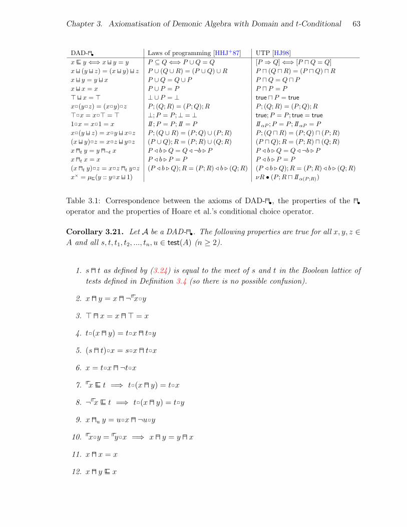
Chapter 3. Axiomatisation of Demonic Algebra with Domain and t-Conditional 63
DAD-G• Laws of programming [HHJ+87] UTP [HJ98]x E y ⇐⇒ x H y = y P ⊆ Q ⇐⇒ P ∪Q = Q [P ⇒ Q] ⇐⇒ [P uQ = Q]x H (y H z) = (x H y) H z P ∪ (Q ∪R) = (P ∪Q) ∪R P u (Q uR) = (P uQ) uR
x H y = y H x P ∪Q = Q ∪ P P uQ = Q u P
x H x = x P ∪ P = P P u P = P
> H x = > ⊥ ∪ P = ⊥ true u P = true
x2(y2z) = (x2y)2z P ; (Q;R) = (P ;Q);R P ; (Q;R) = (P ;Q);R>2x = x2> = > ⊥;P = P ;⊥ = ⊥ true;P = P ; true = true
12x = x21 = x II ;P = P ; II = P II αP ;P = P ; II αP = P
x2(y H z) = x2y H x2z P ; (Q ∪R) = (P ;Q) ∪ (P ;R) P ; (Q uR) = (P ;Q) u (P ;R)(x H y)2z = x2z H y2z (P ∪Q);R = (P ;R) ∪ (Q;R) (P uQ);R = (P ;R) u (Q;R)x Gt y = y G¬t x P / b . Q = Q / ¬b . P P / b . Q = Q / ¬b . P
x Gt x = x P / b . P = P P / b . P = P
(x Gt y)2z = x2z Gt y2z (P / b . Q);R = (P ;R) / b . (Q;R) (P / b . Q);R = (P ;R) / b . (Q;R)x× = µE(y :: y2x H 1) νR • (P ;R u II α(P ;R))
Table 3.1: Correspondence between the axioms of DAD-G•, the properties of the G•
operator and the properties of Hoare et al.’s conditional choice operator.
Corollary 3.21. Let A be a DAD-G•. The following properties are true for all x, y, z ∈A and all s, t, t1, t2, ..., tn, u ∈ test(A) (n ≥ 2).
1. s G t as defined by (3.24) is equal to the meet of s and t in the Boolean lattice of
tests defined in Definition 3.4 (so there is no possible confusion).
2. x G y = x G ¬ppx2y
3. > G x = x G > = x
4. t2(x G y) = t2x G t2y
5. (s G t)2x = s2x G t2x
6. x = t2x G ¬t2x
7. ppx E t =⇒ t2(x G y) = t2x
8. ¬ppx E t =⇒ t2(x G y) = t2y
9. x Gu y = u2x G ¬u2y
10. ppx2y = ppy2x =⇒ x G y = y G x
11. x G x = x
12. x G y E x

Chapter 3. Axiomatisation of Demonic Algebra with Domain and t-Conditional 64
13. (x G y) G z = x G (y G z)
14. x H (y G z) = (x H y) G (x H z)
15. x G (y H z) = (x G y) H (x G z)
16. pp(x G y) = ppx G ppy
17. ppx2ppy = > =⇒ (x G y)2z = x2z G y2z
18. x2z = x ∧ y2z = y =⇒ (x Gt y)2z = x Gt y ∧ (x G y)2z = x G y
19. If t1 G t2 G ... G tn = 1 and t1, t2, ..., tn are pairwise disjoint (n ≥ 2), then
x E y ⇐⇒ t12x E t12y ∧ t22x E t22y ∧ ... ∧ tn2x E tn2y .
Proof :
1. From (3.24), we get
s G t
= 〈 by (3.24) and Proposition 3.14-1 〉
s Gs t
= 〈 by Boolean algebra and Proposition 3.20-3 〉
1 Gs t.
From Definition 3.4, we get
s G t
= 〈 by Proposition 3.20-11 〉
1 Gs t.
2. x G y = x G ¬ppx2y
⇐⇒ 〈 by (3.24) 〉
x Gppx y = x Gppx ¬ppx2y
⇐⇒ 〈 by Proposition 3.20-4 〉
true

Chapter 3. Axiomatisation of Demonic Algebra with Domain and t-Conditional 65
3. > G x
= 〈 by (3.24) and Proposition 3.14-1 〉
> G> x
= 〈 by Proposition 3.20-6 〉
¬>2x
= 〈 by Boolean algebra and (3.7) 〉
x
= 〈 by Propositions 3.20-5 and 3.14-7 〉
x Gppx >= 〈 by (3.24) 〉
x G >
4. t2x G t2y = t2(x G y)
⇐⇒ 〈 by (3.24) 〉
t2x Gpp(t2x) t2y = t2(x Gppx y)
⇐⇒ 〈 by (3.23) 〉
pp(t2x)2t2x = pp(t2x)2t2(x Gppx y) ∧ ¬pp(t2x)2t2y = ¬pp(t2x)2t2(x Gppx y)
⇐⇒ 〈 by Propositions 3.14-9 and 3.14-7, and Boolean algebra 〉
t2x = t2ppx2(x Gppx y) ∧ t2¬ppx2y = t2¬ppx2(x Gppx y)
⇐⇒ 〈 by Propositions 3.20-1 and 3.14-7 〉
true
5. (s G t)2x = s2x G t2x
⇐⇒ 〈 by Proposition 3.20-17 〉
s2(s G t)2x = s2(s2x G t2x) ∧ ¬s2(s G t)2x = ¬s2(s2x G t2x)
⇐⇒ 〈 Boolean algebra, Corollary 3.21-4 and (3.6) 〉
s2x = s2(x G t2x) ∧ ¬s2t2x = > G ¬s2t2x
⇐⇒ 〈 by Corollaries 3.21-2 and 3.21-3 〉
s2x = s2(x G ¬ppx2t2x)
⇐⇒ 〈 by Boolean algebra, Proposition 3.14-17, (3.6) and Corollary
3.21-3 〉true
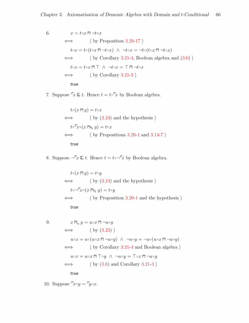
Chapter 3. Axiomatisation of Demonic Algebra with Domain and t-Conditional 66
6. x = t2x G ¬t2x
⇐⇒ 〈 by Proposition 3.20-17 〉
t2x = t2(t2x G ¬t2x) ∧ ¬t2x = ¬t2(t2x G ¬t2x)
⇐⇒ 〈 by Corollary 3.21-4, Boolean algebra and (3.6) 〉
t2x = t2x G > ∧ ¬t2x = > G ¬t2x
⇐⇒ 〈 by Corollary 3.21-3 〉
true
7. Suppose ppx E t. Hence t = t2ppx by Boolean algebra.
t2(x G y) = t2x
⇐⇒ 〈 by (3.24) and the hypothesis 〉
t2ppx2(x Gppx y) = t2x
⇐⇒ 〈 by Propositions 3.20-1 and 3.14-7 〉
true
8. Suppose ¬ppx E t. Hence t = t2¬ppx by Boolean algebra.
t2(x G y) = t2y
⇐⇒ 〈 by (3.24) and the hypothesis 〉
t2¬ppx2(x Gppx y) = t2y
⇐⇒ 〈 by Proposition 3.20-1 and the hypothesis 〉
true
9. x Gu y = u2x G ¬u2y
⇐⇒ 〈 by (3.23) 〉
u2x = u2(u2x G ¬u2y) ∧ ¬u2y = ¬u2(u2x G ¬u2y)
⇐⇒ 〈 by Corollary 3.21-4 and Boolean algebra 〉
u2x = u2x G >2y ∧ ¬u2y = >2x G ¬u2y
⇐⇒ 〈 by (3.6) and Corollary 3.21-3 〉
true
10. Suppose ppx2y = ppy2x.
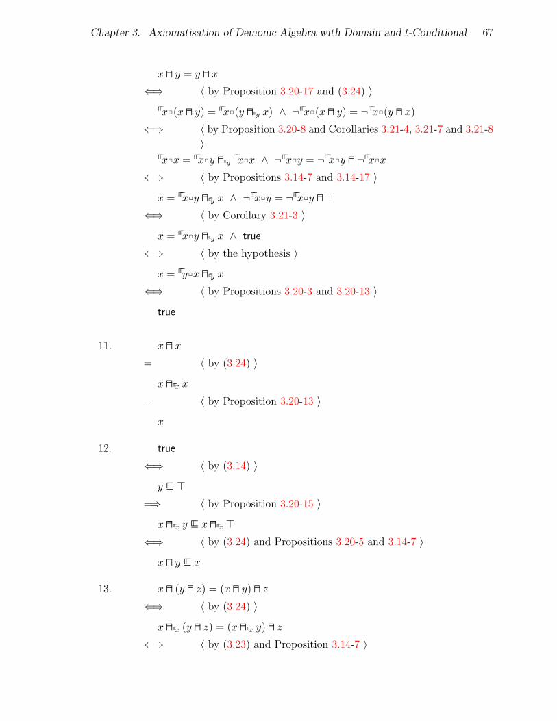
Chapter 3. Axiomatisation of Demonic Algebra with Domain and t-Conditional 67
x G y = y G x
⇐⇒ 〈 by Proposition 3.20-17 and (3.24) 〉
ppx2(x G y) = ppx2(y Gppy x) ∧ ¬ppx2(x G y) = ¬ppx2(y G x)
⇐⇒ 〈 by Proposition 3.20-8 and Corollaries 3.21-4, 3.21-7 and 3.21-8
〉ppx2x = ppx2y Gppy ppx2x ∧ ¬ppx2y = ¬ppx2y G ¬ppx2x
⇐⇒ 〈 by Propositions 3.14-7 and 3.14-17 〉
x = ppx2y Gppy x ∧ ¬ppx2y = ¬ppx2y G >⇐⇒ 〈 by Corollary 3.21-3 〉
x = ppx2y Gppy x ∧ true
⇐⇒ 〈 by the hypothesis 〉
x = ppy2x Gppy x
⇐⇒ 〈 by Propositions 3.20-3 and 3.20-13 〉
true
11. x G x
= 〈 by (3.24) 〉
x Gppx x
= 〈 by Proposition 3.20-13 〉
x
12. true
⇐⇒ 〈 by (3.14) 〉
y E >=⇒ 〈 by Proposition 3.20-15 〉
x Gppx y E x Gppx >⇐⇒ 〈 by (3.24) and Propositions 3.20-5 and 3.14-7 〉
x G y E x
13. x G (y G z) = (x G y) G z
⇐⇒ 〈 by (3.24) 〉
x Gppx (y G z) = (x Gppx y) G z
⇐⇒ 〈 by (3.23) and Proposition 3.14-7 〉
Chapter 3. Axiomatisation of Demonic Algebra with Domain and t-Conditional 68
x = ppx2((x Gppx y) G z) ∧ ¬ppx2(y G z) = ¬ppx2((x Gppx y) G z)
⇐⇒ 〈 by Corollaries 3.21-7 and 3.21-4, Proposition 3.20-20, (3.24)
and Boolean algebra 〉x = ppx2(x Gppx y) ∧ ¬ppx2y G ¬ppx2z = ¬ppx2(x Gppx y) G ¬ppx2z
⇐⇒ 〈 by Propositions 3.20-1 and 3.14-7 〉
true
14. (x H y) G (x H z) = x H (y G z)
⇐⇒ 〈 by (3.24), (3.21) and Proposition 3.14-3 〉
(x H y) Gppx2ppy (x H z) = x H (y G z)
⇐⇒ 〈 by (3.23), Proposition 3.14-11 and De Morgan 〉
x H y = ppx2ppy2(x H (y G z)) ∧(¬ppx G ¬ppy)2(x H z) = (¬ppx G ¬ppy)2(x H (y G z))
⇐⇒ 〈 by (3.8), Corollary 3.21-7 and Propositions 3.14-11 and 3.14-7
〉true ∧ (¬ppx G ¬ppy)2(x H z) = (¬ppx G ¬ppy)2(x H (y G z))
⇐⇒ 〈 by Propositions 3.14-7 and 3.14-20, and Boolean algebra 〉
¬ppy2(x H z) = ¬ppy2(x H (y G z))
⇐⇒ 〈 by (3.8) and Corollary 3.21-8 〉
true
15. x G (y H z)
= 〈 by (3.24) 〉
x Gppx (y H z)
= 〈 by Proposition 3.20-9 〉
(x Gppx y) H (x Gppx z)
= 〈 by (3.24) 〉
(x G y) H (x G z)
16. pp(x G y)
= 〈 by (3.24) 〉
pp(x Gppx y)
= 〈 by Proposition 3.20-20 〉
ppx Gppx ppy
Chapter 3. Axiomatisation of Demonic Algebra with Domain and t-Conditional 69
= 〈 by Proposition 3.14-1 and (3.24) 〉
ppx G ppy
17. Suppose ppx2ppy = >, hence ¬ppx2ppy = ppy by Boolean algebra.
(x G y)2z
= 〈 by (3.24) 〉
(x Gppx y)2z
= 〈 by Proposition 3.20-7 〉
x2z Gppx y2z
= 〈 by Corollary 3.21-9, Proposition 3.14-7 and the hypothesis 〉
x2z G y2z
18. Suppose x2z = x and y2z = y.
(x Gt y)2z
= 〈 by Proposition 3.20-7 〉
x2z Gt y2z
= 〈 by the hypothesis 〉
x Gt y
(x G y)2z
= 〈 by (3.24) 〉
(x Gppx y)2z
= 〈 see the previous derivation 〉
x Gppx y
= 〈 by (3.24) 〉
x G y
19. We prove Corollary 3.21-19 by induction.
Basis case n = 2. For any t1 and t2 such that t1 G t2 = 1 and t12t2 = >, t2 = ¬t1by Boolean algebra. Thus, Proposition 3.20-16 gives
x E y ⇐⇒ t12x E t12y ∧ t22x E t22y .
Chapter 3. Axiomatisation of Demonic Algebra with Domain and t-Conditional 70
Induction hypothesis. Suppose that for any t1, t2, ..., tn−1 such that t1 G t2 G ... G
tn−1 = 1 and t1, t2, ..., tn−1 are pairwise disjoint,
x E y ⇐⇒ t12x E t12y ∧ t22x E t22y ∧ ... ∧ tn−12x E tn−12y .
Suppose now that t1 G t2 G ...G tn = 1 and t1, t2, ..., tn are pairwise disjoint. Then
(t1 G t2) G t3 G ... G tn = 1 and (t1 G t2), t3, ..., tn are pairwise disjoint by Boolean
algebra.
x E y
⇐⇒ 〈 by the induction hypothesis 〉
(t1 G t2)2x E (t1 G t2)2y ∧ t32x E t32y ∧ ... ∧ tn2x E tn2y
⇐⇒ 〈 by Proposition 3.20-16, the hypothesis and Boolean algebra 〉
t12x E t12y ∧ t22x E t22y ∧ ... ∧ tn2x E tn2y
2
By Corollary 3.21-14 and (3.2), (xG y) H z = (xH z) G (y H z). However, (xH y) G z =
(xGz)H(yGz) is false in general. Take the relations x = {(0, 0)}, y = {} and z = {(0, 1)}as a counter-example.
Furthermore, the equality (x G y)2z = x2z G y2z is also false in general (com-
pare with Proposition 3.20-7). Take the relations x = {(0, 0), (0, 1), (1, 0), (1, 1)},y = {(0, 1), (1, 1)} and z = {(1, 1)} as a counter-example. This counter-example
shows that the hypothesis of Corollary 3.21-17 is welcome. Another way of getting
(x G y)2z = x2z G y2z is to focus on tests, as in Corollary 3.21-5.
In order to demonstrate a refinement x E y for x, y ∈ A, rather than deriving it
directly, it is sometimes easier to break it in more refinements t12x E t12y, t22x E t22y,
..., tn2x E tn2y. This can be done under suitable hypotheses thanks to Corollary 3.21-
19. This case analysis with many tests is going to be used several times in the proof of
Theorem 4.31.
There is a trivial and very useful contraction of Proposition 3.14-21 and Corol-
lary 3.21-10 which reads
ppx2ppy = > =⇒ x G y = y G x . (3.25)
By Corollary 3.21-12, x G y E x. In general, x G y E y does not hold. Take the
relations x = {(0, 0)} and y = {(0, 1)} as a counter-example. However it is true under
Chapter 3. Axiomatisation of Demonic Algebra with Domain and t-Conditional 71
suitable hypotheses. The following lemma presents hypotheses that help manipulating
G operators involved in different refinements.
Lemma 3.22. Let A be a DAD-G•. The following properties are true for all x, y, z ∈ A.
1. y E z =⇒ x G y E x G z
2. x E y =⇒ x E y G x
3. x E y ∧ ppx = ppy =⇒ x G z E y G z
4. x E y ∧ ppx2ppz = > =⇒ x G z E y G z
5. pp(x G y) = ppz ∧ x = ppx2z ∧ y = ppy2z =⇒ x G y = z
6. x E y G z ⇐⇒ x E y ∧ x E ¬ppy2z
7. ppx2ppy = ppw2ppz = > =⇒ (w G x) H (y G z) = (w H y) G (x H z)
Proof :
1. This follows from (3.24) and Proposition 3.20-15.
2. Suppose x E y
y G x
= 〈 by Corollary 3.21-2 〉
y G ¬ppy2x
= 〈 by Proposition 3.14-9 and Boolean algebra,
ppy2pp(¬ppy2x) = >,
then apply (3.25) 〉¬ppy2x G y
= 〈 by Proposition 3.14-7 〉
¬ppy2x G ppy2y
F 〈 by the hypothesis and Lemma 3.22-1 〉
¬ppy2x G ppy2x
= 〈 by Corollary 3.21-6 〉
x

Chapter 3. Axiomatisation of Demonic Algebra with Domain and t-Conditional 72
3. This follows from (3.24) and Proposition 3.20-14.
4. Assume ppx2ppz = >.
x G z E y G z
⇐⇒ 〈 by Proposition 3.20-16 〉
ppx2(x G z) E ppx2(y G z) ∧ ¬ppx2(x G z) E ¬ppx2(y G z)
⇐⇒ 〈 by Corollaries 3.21-7, 3.21-8 and 3.21-4, and Proposition
3.14-7 〉ppx2x E ppx2y G ppx2ppz2z ∧ ¬ppx2ppz2z E ¬ppx2ppy2y G ¬ppx2ppz2z
⇐⇒ 〈 by the hypothesis, Boolean algebra, (3.6), Corollary 3.21-3
and Proposition 3.14-7 〉ppx2x E ppx2y ∧ z E ¬ppx2y G z
⇐= 〈 by Proposition 3.14-8, Boolean algebra, (3.6) and Corollary
3.21-3 〉x E y
5. Assume x = ppx2z, y = ppy2z and pp(x G y) = ppz. Hence,
¬ppx2ppy = ¬ppx2ppz (3.26)
by Corollary 3.21-16 and Boolean algebra.
x G y = z
⇐⇒ 〈 by (3.24) 〉
x Gppx y = z
⇐⇒ 〈 by (3.23) and Proposition 3.14-7 〉
x = ppx2z ∧ ¬ppx2y = ¬ppx2z
⇐⇒ 〈 by the hypothesis 〉
true ∧ ¬ppx2ppy2z = ¬ppx2z
⇐⇒ 〈 by Proposition 3.14-7 and (3.26) 〉
true
6. x E y G z
⇐⇒ 〈 by (3.24) 〉
x E y Gppy z
⇐⇒ 〈 by Propositions 3.20-18 and 3.14-7 〉
x E y ∧ x E ¬ppy2z

Chapter 3. Axiomatisation of Demonic Algebra with Domain and t-Conditional 73
7. Assume ppx2ppy = > and ppw2ppz = >.
(w G x) H (y G z)
= 〈 by Corollary 3.21-14 〉
((w G x) H y) G ((w G x) H z)
= 〈 by (3.2) and Corollary 3.21-14 〉
(w H y) G (x H y) G (w H z) G (x H z)
= 〈 by Proposition 3.14-11, the hypothesis, (3.6) and
Corollary 3.21-3 〉(w H y) G (x H z)
2
Propositions 3.20-21 and 3.14-7 with Definition 3.24 imply that xGy is the infimum
of x and ¬ppx2y with respect to E.

Chapter 4
Definition of Angelic Operators in
DAD
As mentioned at the beginning of Section 3.4, we are looking for a downward link —
refer to Figure 1.4— from DAD-G• to KAD for any model of KAD. The idea is to define
angelic operators in the context of DAD-G• and then demonstrate that the elements of
a DAD-G• together with those angelic operators form a KAD. This is exactly what is
done in this chapter.
In Sections 4.1, 4.2 and 4.3, we respectively define angelic non-deterministic choice
+D, angelic sequential composition ·D and angelic finite iteration ∗D . In Section 4.2,
we also define decomposable elements. These are indispensable for the definition of the
·D operator. In Section 4.4, we demonstrate many properties about decomposable ele-
ments. Finally, in Section 4.5, we demonstrate that the elements of a DAD-G• together
with those angelic operators form a KAD. This last result of the chapter is one of the
most important of this thesis. Indeed, it is the second step toward the desired duality
(refer to Section 1.3).
We add a subscript D to the angelic operators defined here, to denote that they are
defined by demonic expressions.

Chapter 4. Definition of Angelic Operators in DAD 75
4.1 Angelic Refinement and Angelic Choice
We start with the angelic partial order ≤D. It is easy to see that this definition is the
demonic version of Definition 2.9.
Definition 4.1 (Angelic refinement). Let A be a DAD-G• and take x, y ∈ A. We say
that x≤D y when
ppy E ppx , (4.1)
x E ppx2y . (4.2)
Proposition 4.3 below states that ≤D is a partial order. Moreover, it gives a formula
using demonic operators for the angelic supremum with respect to this partial order.
In order to demonstrate this proposition, we need the following lemma.
Lemma 4.2. Let A be a DAD-G•. The function
f : A× A −→ A
(x, y) 7→ (x H y) G ¬ppy2x G ¬ppx2y
satisfies the following four properties for all x, y, z ∈ A. Note that f is well defined by
Corollary 3.21-13.
1. ppf(x, y) = ppx G ppy
2. f(x, x) = x
3. f(x, y) = f(y, x)
4. f(x, f(y, z)) = f(f(x, y), z)
Proof :
1. ppf(x, y)
= 〈 by definition of f 〉
pp((x H y) G ¬ppy2x G ¬ppx2y)
= 〈 by Corollary 3.21-16 〉
pp(x H y) G pp(¬ppy2x) G pp(¬ppx2y)
Chapter 4. Definition of Angelic Operators in DAD 76
= 〈 by (3.21) and Propositions 3.14-3 and 3.14-9 〉
ppx2ppy G ¬ppy2ppx G ¬ppx2ppy
= 〈 by Boolean algebra 〉
ppx G ppy
2. f(x, x)
= 〈 by definition of f 〉
(x H x) G ¬ppx2x G ¬ppx2x
= 〈 by Proposition 3.14-17 〉
(x H x) G > G >= 〈 by Corollary 3.21-3 and (3.3) 〉
x
3. f(x, y)
= 〈 by definition of f 〉
(x H y) G ¬ppy2x G ¬ppx2y
= 〈 by Proposition 3.14-9 and Boolean algebra,
pp(¬ppy2x)2pp(¬ppx2y) = ¬ppy2ppx2¬ppx2ppy = >,
then apply (3.2) and (3.25) 〉(y H x) G ¬ppx2y G ¬ppy2x
= 〈 by definition of f 〉
f(y, x)
4. Here is the derivation. It repeatedly invokes (3.25). Using (3.21), Boolean algebra
and Proposition 3.14-9, it is easy to check that the operands of the various G
operators are pairwise disjoint, so that the condition ppx2ppy = > of (3.25) is
satisfied. This is what allows permuting the operands.
f(x, f(y, z))
= 〈 by definition of f and Lemma 4.2-1 〉
(x H ((y H z) G ¬ppz2y G ¬ppy2z))G
¬(ppy G ppz)2x G ¬ppx2((y H z) G ¬ppz2y G ¬ppy2z)
= 〈 by Corollaries 3.21-14 and 3.21-4, and Boolean algebra 〉
(x H y H z) G (x H ¬ppz2y) G (x H ¬ppy2z) G
¬ppy2¬ppz2x G ¬ppx2(y H z) G ¬ppx2¬ppz2y G ¬ppx2¬ppy2z
Chapter 4. Definition of Angelic Operators in DAD 77
= 〈 by Proposition 3.14-20 and (3.25) 〉
(x H y H z) G ¬ppz2(x H y) G ¬ppy2(x H z) G ¬ppx2(y H z) G
¬ppy2¬ppz2x G ¬ppx2¬ppz2y G ¬ppx2¬ppy2z
= 〈 by (3.2), (3.21), Proposition 3.14-9, (3.25) and Boolean algebra
〉(z H x H y) G ¬ppy2(z H x) G ¬ppx2(z H y) G ¬ppz2(x H y) G
¬ppx2¬ppy2z G ¬ppz2¬ppy2x G ¬ppz2¬ppx2y
= 〈 by Proposition 3.14-20 and (3.25) 〉
(z H x H y) G (z H ¬ppy2x) G (z H ¬ppx2y) G ¬ppx2¬ppy2z G
¬ppz2(x H y) G ¬ppz2¬ppy2x G ¬ppz2¬ppx2y
= 〈 by Corollaries 3.21-14 and 3.21-4, and Boolean algebra 〉
(z H ((x H y) G ¬ppy2x G ¬ppx2y)) G ¬(ppx G ppy)2z G
¬ppz2((x H y) G ¬ppy2x G ¬ppx2y)
= 〈 by definition of f and Lemma 4.2-1 〉
f(z, f(x, y))
= 〈 by Lemma 4.2-3 〉
f(f(x, y), z)
2
Proposition 4.3 (Angelic choice). The angelic refinement of Definition 4.1 satisfies
the following three properties.
1. For all x, >≤D x.
2. For all x, y,
x≤D y ⇐⇒ f(x, y) = y ,
where f is the function defined in Lemma 4.2.
3. ≤D is a partial order. Letting x+D y denote the supremum of x and y with respect
to ≤D, we have
x+D y = f(x, y) .
Proof :

Chapter 4. Definition of Angelic Operators in DAD 78
1. From (3.14) and Proposition 3.14-8, we have ppx E pp>. Also, from Proposition
3.14-1 and (3.6), pp>2x = >, so > E pp>2x. These two refinements are those from
Definition 4.1, so >≤D x.
2. f(x, y) = y
⇐⇒ 〈 by Propositions 3.20-17, 3.14-7 and 3.14-17 〉
ppy2f(x, y) = y ∧ ¬ppy2f(x, y) = >⇐⇒ 〈 by Proposition 3.20-17 and (3.6) 〉
ppx2ppy2f(x, y) = ppx2y ∧ ppx2¬ppy2f(x, y) = > ∧¬ppx2ppy2f(x, y) = ¬ppx2y ∧ ¬ppx2¬ppy2f(x, y) = >
⇐⇒ 〈 by definition of f , Corollaries 3.21-4 and 3.21-3, Propositions
3.14-7, 3.14-17 and 3.14-11, Boolean algebra and (3.6) 〉ppx2ppy2(x H y) = ppx2y ∧ ¬ppy2x = > ∧ ¬ppx2y = ¬ppx2y ∧ > = >
⇐⇒ 〈 by Proposition 3.14-11 and Boolean algebra 〉
ppx2(x H y) = ppx2y ∧ ¬ppy2x = >⇐⇒ 〈 by Propositions 3.14-20, 3.14-7, 3.14-19 and 3.14-9 〉
x H ppx2y = ppx2y ∧ ¬ppy2ppx = >⇐⇒ 〈 by Proposition 3.14-16 〉
x H ppx2y = ppx2y ∧ ppy E ppx
⇐⇒ 〈 by (3.11) and Definition 4.1 〉
x≤D y
3. It follows from the previous point of the present proposition and by the fact that
f is reflexive, symmetric and transitive (see Lemma 4.2). 2
Proposition 4.3 and Lemma 4.2 show that ≤D and +D do what we expect them to
do and the following corollary is a direct consequence of these results.
Corollary 4.4. Let A be a DAD-G•. For all x, y, z ∈ A,
1. x+D y = (x H y) G ¬ppy2x G ¬ppx2y,
2. ≤D is a partial order and x+D y = y ⇐⇒ x≤D y,
3. pp(x+D y) = ppx G ppy,
4. (x+D y) +D z = x+D (y +D z),
Chapter 4. Definition of Angelic Operators in DAD 79
5. x+D y = y +D x,
6. x+D x = x,
7. >+D x = x+D > = x.
Remark 4.5. Note that for all s, t ∈ test(A),
s≤D t ⇐⇒ t E s
by Definition 4.1, Proposition 3.14-1 and Boolean algebra. This equivalence is the
demonic version of the one of Remark 2.11.
Remark 4.6. Since the domains of x H y, ¬ppx2y and ¬ppy2x are pairwise disjoint by
(3.21) and Proposition 3.14-9, the three terms in the definition of f (see Lemma 4.2)
commute. In the next sections and chapters, we will use any of the following equalities
by refering to Corollary 4.4-1.
x+D y = (x H y) G ¬ppy2x G ¬ppx2y
x+D y = (x H y) G ¬ppx2y G ¬ppy2x
x+D y = ¬ppy2x G ¬ppx2y G (x H y)
x+D y = ¬ppy2x G (x H y) G ¬ppx2y
x+D y = ¬ppx2y G ¬ppy2x G (x H y)
x+D y = ¬ppx2y G (x H y) G ¬ppy2x
Other major properties of +D will be presented in Section 4.5.
4.2 Angelic Composition and Demonic Decomposi-
tion
We now turn to the definition of angelic composition. But things are not as simple as
for ≤D or +D. The difficulty is due to the asymmetry between left and right caused by
the difference between Proposition 3.20-7 and 3.20-8, and by the absence of a codomain
operator for “testing” the right-hand side of elements as can be done with the domain
operator on the left. Consider the relations
Q = {(0, 0), (0, 1), (1, 2), (2, 3)} ,
R = {(0, 0), (2, 2)} .

Chapter 4. Definition of Angelic Operators in DAD 80
The angelic composition of Q and R is Q · R = {(0, 0), (1, 2)}, while their demonic
composition is Q2R = {(1, 2)}. There is no way to express Q ·R only in terms of Q2R.
What we could try to do is to decompose Q as follows using the conditional operator:
Q = Q2ppR G Q2¬ppR G (Q1 H Q2) ,
where Q1 = {(0, 0)} and Q2 = {(0, 1)}. Note that Q2ppR = {(1, 2)} and Q2¬ppR =
{(2, 3)}, so that the domains of the three operands of G are disjoint. The effect of G is
then just union. With these relations, it is possible to express the angelic composition
as Q ·R = Q2RGQ12R. Now, it is possible to extract Q1 HQ2 from Q, since Q1 HQ2 =
¬pp(Q2ppR)2¬pp(Q2¬ppR)2Q. The problem is that it is not possible to extract Q1 from
Q1 HQ2. On the one hand, Q1 and Q2 have the same domain; on the other hand, there
is no test t such that Q1 = (Q1 H Q2)2t. This is what leads to the following definition.
Definition 4.7 (Decomposition). Let A be a DAD-G• and take t ∈ test(A). An element
x ∈ A is said to be t-decomposable if and only if there are unique elements xt and x¬tsuch that
x = x2t G x2¬t G (xt H x¬t) , (4.3)
pp(xt) = pp(x¬t) = ¬pp(x2t)2¬pp(x2¬t)2ppx , (4.4)
xt = xt2t , (4.5)
x¬t = x¬t2¬t . (4.6)
Moreover, x is said to be decomposable if and only if it is t-decomposable for all t ∈test(A).
Remark 4.8. The domains pp(x2t), pp(x2¬t) and pp(xt) (or pp(x¬t)) obtained by decom-
posing x as in Definition 4.7 are pairwise disjoint. That pp(xt) and pp(x¬t) are disjoint
from pp(x2t) and pp(x2¬t) is obvious from (4.4). By Lemma 3.17-4, pp(x2t) and pp(x2¬t)are disjoint as well. This disjointness is often used in applications of (3.25) and Corol-
lary 3.21-17.
Moreover,
ppx = pp(x2t) G pp(x2¬t) G pp(xt) , (4.7)
since
pp(x2t) G pp(x2¬t) G pp(xt)
= 〈 by (4.4) 〉
pp(x2t) G pp(x2¬t) G ¬pp(x2t)2¬pp(x2¬t)2ppx

Chapter 4. Definition of Angelic Operators in DAD 81
= 〈 by Boolean algebra 〉
pp(x2t) G pp(x2¬t) G ppx
= 〈 by Proposition 3.14-18 and Boolean algebra 〉
ppx .
Then from Corollary 3.21-16, Boolean algebra and Remark 4.8, it is easy to see that
pp(x2t G xt) = ¬pp(x2¬t)2ppx , (4.8)
ppx E pp(x2t G xt) , (4.9)
¬ppx2xt = > . (4.10)
Remark 4.9. Any element x ∈ A is 1-decomposable and >-decomposable. Indeed,
x1 = x> = >
by (4.4), Boolean algebra, (3.6) and Propositions 3.14-1 and 3.14-19.
Looking at Definition 4.7, many questions arise. Before defining angelic composition,
we answer them.
• Are demonic tests all decomposable?
Indeed they are, the t-decomposition of a test s is
s = s2t G s2¬t G (> H >) (4.11)
by (4.4), Boolean algebra and Propositions 3.14-1 and 3.14-19.
• Is there a DAD-G• containing an element that is not decomposable?
The following example presents such a scenario.
Example 4.10. For this example, we consider the following nine relations defined
on S2 = {1, 2}.
> =
(0 0
0 0
)s =
(1 0
0 0
)t =
(0 0
0 1
)1 =
(1 0
0 1
)
a =
(1 0
1 1
)b =
(1 1
0 1
)c =
(1 1
1 1
)d =
(1 1
0 0
)e =
(0 0
1 1
)

Chapter 4. Definition of Angelic Operators in DAD 82
>
����
���
>>>>
>>>>
d
����
����
????
????
e
����
����
====
====
s
====
====
c
����
����
????
????
t
����
����
a
????
???? b
����
����
1
Figure 4.1: Hasse diagram of Example 4.10.
Take A = {>, s, t, 1, a, b, c, d, e}, test(A) = {>, s, t, 1} and the demonic operators
defined by the following tables, omitting G•.
H > s t 1 a b c d e
> > > > > > > > > >s > s > s s d d d >t > > t t e t e > e
1 > s t 1 a b c d e
a > s e a a c c d e
b > d t b c b c d e
c > d e c c c c d e
d > d > d d d d d >e > > e e e e e > e
2 > s t 1 a b c d e
> > > > > > > > > >s > s > s s d d d >t > > t t e t e > e
1 > s t 1 a b c d e
a > s > a a c c d >b > > t b c b c > e
c > > > c c c c > >d > > > d d d d > >e > > > e e e e > >
×
> >s s
t t
1 1
a a
b b
c c
d >e >
pp
> >s s
t t
1 1
a 1
b 1
c 1
d s
e t
¬> 1
s t
t s
1 >
The demonic refinement ordering corresponding to H is represented in the semi-
lattice of Figure 4.1. It is easy to convince oneself that it is a DAD-G•. Look
at Figure 2.3. The present example is simply a subalgebra of that figure. The

Chapter 4. Definition of Angelic Operators in DAD 83
elements a, b, c, d and e are not decomposable. For instance, to decompose c with
respect to s would require the existence of the relations
f =
(1 0
1 0
)and g =
(0 1
0 1
),
which are not there.
• Let t be a demonic test. May an element of a DAD-G• have more than one t-
decomposition? In other words, is it relevant to ask for uniqueness in Definition
4.7?
Example 4.12 is one where there is an element with nine different t-decomposi-
tions. This example is constructed from the general structure introduced in the
following lemma.
Lemma 4.11. Let (A, test(A),H, 2, ×,>, 1,¬,G, pp ,G•) be a DAD-G•. Consider
E = {(x, t) : A× test(A) | ppx E t} and T = {(t, t) : test(A)× test(A)} and define
the following operations for elements of E, where x, y ∈ A and s, t, u ∈ test(A).
(x, s)⊕ (y, t) = (x H y, s H t)
(x, s)� (y, t) = (x2y, pp(s2x2t))
(x, s)~ = (x×, pp(x×2s))
(s, s) = (¬s,¬s)(s, s) e (t, t) = (s G t, s G t)
pp(x, s) = (ppx, ppx)
(x, s) e(u,u) (y, t) = (x Gu y, s Gu t)
Then (E, T,⊕,�, ~, (>,>), (1, 1), ,e, pp,e•) is a DAD-e• and the partial order
related to ⊕ satisfies
(x, s) E (y, t) ⇐⇒ x E y ∧ s E t .
Proof : The proof of Lemma 4.11 contains no new idea and is ten pages long.
Therefore, it is postponed to Appendix A. 2
Here is a DAD-G• where the t-decomposition of x is not unique.
Example 4.12. Take the structure constructed in Lemma 4.11 with relations on
the set S2 = {1, 2} as carrier set A. Take the following relations
> =
(0 0
0 0
)s =
(1 0
0 0
)t =
(0 0
0 1
)1 =
(1 0
0 1
)f =
(1 0
1 0
)g =
(0 1
0 1
)c =
(1 1
1 1
)

Chapter 4. Definition of Angelic Operators in DAD 84
and define C = (>,>). Then (c,>) admits nine different (s, s)-decompositions.
(c,>) = C e C e ((f,>)⊕ (g,>)) (4.12)
(c,>) = C e C e ((f, s)⊕ (g, t)) (4.13)
(c,>) = C e C e ((f, t)⊕ (g, s)) (4.14)
(c,>) = C e C e ((f, s)⊕ (g,>)) (4.15)
(c,>) = C e C e ((f, t)⊕ (g,>)) (4.16)
(c,>) = C e C e ((f,>)⊕ (g, s)) (4.17)
(c,>) = C e C e ((f,>)⊕ (g, t)) (4.18)
(c,>) = C e C e ((f, 1)⊕ (g,>)) (4.19)
(c,>) = C e C e ((f,>)⊕ (g, 1)) (4.20)
Lemma 4.11 is going to be used in Section 6.1 in order to give a possible semantics
for DAD-G• containing nondecomposable elements.
• Do the decomposable elements of a DAD-G• A together with the demonic opera-
tors form a subalgebra of A?
The answer is no and here is a counter-example. Go back to Example 4.12. It is
easy to see that the elements (f, s) and (g, t) are (s, s)-decomposable, because
(f, s) = (f, s) e C e (C ⊕ C)
(g, t) = C e (g, t) e (C ⊕ C)
since
(f, s) = (f, s)� (s, s)
(g, t) = (g, t)� (s, s) .
For the same reason, (f, s) and (g, t) are (t, t)-decomposable. Also, (f, s) and (g, t)
are (1, 1)-decomposable and C-decomposable by Remark 4.9. Therefore, (f, s) and
(g, t) are decomposable.
However, (f, s) ⊕ (g, t) has two possible (s, s)-decompositions (see (4.13) and
(4.14)):
(f, s)⊕ (g, t) = (c,>) = C e C e ((f, s)⊕ (g, t))
(f, s)⊕ (g, t) = (c,>) = C e C e ((f, t)⊕ (g, s)) .
So (f, s)⊕ (g, t) is not decomposable, while (f, s) and (g, t) are.
• Therefore, are there maximal subalgebras of decomposable elements?
Fortunately, the answer is yes. It is the subject of the following proposition.
Chapter 4. Definition of Angelic Operators in DAD 85
Proposition 4.13 (Maximal subalgebra of decomposable elements). Let A be a
DAD-G•. There is a maximal subalgebra (not necessarily unique) of decomposable
elements containing test(A).
The proof of Proposition 4.13 involves Zorn’s Lemma (which is equivalent to the
axiom of choice, see [Jec73]) and here is how it reads.
Lemma 4.14 (Zorn’s Lemma). Every non-empty partially ordered set in which
every chain has an upper bound contains at least one maximal element.
Now let us prove Proposition 4.13. To ease the presentation of the proof, we make
no distinction between a DAD-G• and its carrier set.
Proof : Consider
E = {I : ℘(A) | test(A) ⊆ I ∧ I is a subalgebra of decomposable elements} .
Since all tests are decomposable (see (4.11)), test(A) ∈ E so E is not empty.
Trivially, E is partially ordered by inclusion.
Let C ⊆ E be a chain. We will demonstrate that
IC =⋃I∈C
I
is an upper bound for C. Then, by Zorn’s Lemma, the proof is done.
Take x, y, t ∈ IC . There are I ′, I ′′, I ′′′ ∈ C such that x ∈ I ′, y ∈ I ′′ and t ∈ I ′′′.
Without loss of generality, I ′ ⊆ I ′′ ⊆ I ′′′ so x, y, t ∈ I ′′′. Then, since I ′′′ is a
subalgebra of decomposable elements, xH y, x2y, x× and xGt y are decomposable
and belong to I ′′′ and thus to IC . Since, for all I ∈ C, test(A) ⊆ I, then test(A) ⊆IC . Therefore, IC is an upper bound for C. 2
That proposition brings back confidence in the concept of decomposition. Indeed,
considering any DAD-G• A, Proposition 4.13 guarantees that there is a part of Acontaining test(A) that is a subalgebra of decomposable elements. If A is itself
a subalgebra of decomposable elements containing test(A), then we say that A is
an algebra of decomposable elements.
Definition 4.15 (Algebra of decomposable elements). A DAD-G• A is an algebra
of decomposable elements if x is decomposable for all x ∈ A.
In Section 4.4, we will consider algebras of decomposable elements and study
many of their properties. In Section 4.5, we will show that the elements of an
algebra of decomposable elements together with the angelic operators defined
in Sections 4.1, 4.2 and 4.3 form a KAD. In Chapter 5, we will demonstrate
that this result of Section 4.5 can only be valid within algebras of decomposable
elements. We will also demonstrate that all KAD-based DAD-G•s are algebras of
decomposable elements.

Chapter 4. Definition of Angelic Operators in DAD 86
We are now ready to define angelic composition.
Definition 4.16 (Angelic composition). Let x and y be elements of a DAD-G• such
that x is ppy-decomposable. The angelic composition x ·D y is defined by
x ·D y = x2y G xppy2y .
Proposition 4.17. Let x, y, z be elements of a DAD-G• A. Then
1. 1 ·D x = x ·D 1 = x,
2. > ·D x = x ·D > = >,
3. t ·D x = t2x,
4. ppy = 1 =⇒ x ·D y = x2y.
5. If x is ppy-decomposable, then pp(x ·D y) = ppx2¬pp(x2¬ppy).
6. If x is ppy-decomposable and pp(y ·D z)-decomposable, y is ppz-decomposable and x ·D yis ppz-decomposable, then pp(x ·D (y ·D z)) = pp((x ·D y) ·D z).
7. If x is ppy-decomposable, then x ·D y = (x2ppy G xppy)2y.
The hypotheses of Propositions 4.17-5, 4.17-6 and 4.17-7 ensure that each angelic
composition involved is well defined. There is no need for such assumptions for Propo-
sitions 4.17-1, 4.17-2, 4.17-3 and 4.17-4 since all tests are decomposable by (4.11) and
any element is 1-decomposable and >-decomposable by Remark 4.9.
These comments illustrate how careful one must be when dealing with angelic com-
position. However, in further sections, when decomposition is involved, we will suppose
that A is an algebra of decomposable elements. Therefore, all angelic compositions will
be well defined.
Proof :
1. 1 ·D x= 〈 by Definition 4.16 〉
12x G 1ppx2x
= 〈 by (4.11) 〉
12x G >2x
Chapter 4. Definition of Angelic Operators in DAD 87
= 〈 by (3.7), (3.6) and Corollary 3.21-3 〉
x
= 〈 by (3.7) and Corollary 3.21-3 〉
x21 G >21
= 〈 by Remark 4.9 and Proposition 3.14-1 〉
x21 G xpp121
= 〈 by Definition 4.16 〉
x ·D 1
2. > ·D x= 〈 by Definition 4.16 〉
>2x G >ppx2x
= 〈 by (4.11) 〉
>2x G >2x
= 〈 by (3.6) and Corollary 3.21-11 〉
>= 〈 by (3.6) and Corollary 3.21-11 〉
x2> G >2>= 〈 by Remark 4.9 and Proposition 3.14-1 〉
x2> G xpp>2>= 〈 by Definition 4.16 〉
x ·D >
3. t ·D x= 〈 by Definition 4.16 〉
t2x G tppx2x
= 〈 by (4.11) 〉
t2x G >2x
= 〈 by (3.6) and Corollary 3.21-3 〉
t2x
4. Suppose ppy = 1
x ·D y
Chapter 4. Definition of Angelic Operators in DAD 88
= 〈 by Definition 4.16, the hypothesis and Remark 4.9 〉
x2y G x12y
= 〈 by Remark 4.9 〉
x2y G >2y
= 〈 by (3.6) and Corollary 3.21-3 〉
x2y
5. Suppose x is ppy-decomposable.
pp(x ·D y)= 〈 by Definition 4.16, Corollary 3.21-16 and (3.20) 〉
pp(x2ppy) G pp(xppy2ppy)
= 〈 by (4.5) with x, t := x, ppy 〉
pp(x2ppy) G pp(xppy)
= 〈 by (4.4) with x, t := x, ppy 〉
pp(x2ppy) G ¬pp(x2ppy)2¬pp(x2¬ppy)2ppx
= 〈 by Boolean algebra 〉
pp(x2ppy) G ¬pp(x2¬ppy)2ppx
= 〈 by Boolean algebra, Lemma 3.17-5 and Proposition 3.14-18,
¬pp(x2¬ppy)2ppx E pp(x2ppy) ⇐⇒¬pp(x2¬ppy) E pp(x2ppy) ∧ ppx E pp(x2ppy) ⇐⇒ true,
then apply Boolean algebra 〉ppx2¬pp(x2¬ppy)
6. Suppose x is ppy-decomposable and pp(y ·D z)-decomposable, y is ppz-decomposable
and x ·D y is ppz-decomposable.
pp(x ·D (y ·D z))= 〈 by Proposition 4.17-5 〉
ppx2¬pp(x2¬(ppy2¬pp(y2¬ppz)))
= 〈 by De Morgan 〉
ppx2¬pp(x2(¬ppy G pp(y2¬ppz)))
= 〈 by (4.3) with x, t := x, ppy 〉
ppx2¬pp((x2ppy G x2¬ppy G (xppy H x¬ppy))2(¬ppy G pp(y2¬ppz)))

Chapter 4. Definition of Angelic Operators in DAD 89
= 〈 by Corollary 3.21-17 and Remark 4.8 〉
ppx2¬pp(x2ppy2(¬ppy G pp(y2¬ppz)) G x2¬ppy2(¬ppy G pp(y2¬ppz)) G
(xppy H x¬ppy)2(¬ppy G pp(y2¬ppz)))
= 〈 by Corollaries 3.21-8 and 3.21-7, and Boolean algebra 〉
ppx2¬pp(x2ppy2pp(y2¬ppz) G x2¬ppy G (xppy H x¬ppy)2(¬ppy G pp(y2¬ppz)))
= 〈 by Proposition 3.14-18 and Boolean algebra 〉
ppx2¬pp(x2pp(y2¬ppz) G x2¬ppy G (xppy H x¬ppy)2(¬ppy G pp(y2¬ppz)))
= 〈 by Corollary 3.21-16 and (3.20) 〉
ppx2¬pp(x2y2¬ppz G x2¬ppy G (xppy H x¬ppy)2(¬ppy G pp(y2¬ppz)))
= 〈 by (4.5) with x, t := x, ppy, (4.6) with x, t := x, ppy and (3.9) 〉
ppx2¬pp(x2y2¬ppz G x2¬ppy G
(xppy2ppy2(¬ppy G pp(y2¬ppz)) H x¬ppy2¬ppy2(¬ppy G pp(y2¬ppz))))
= 〈 by Corollaries 3.21-8 and 3.21-7, and Boolean algebra 〉
ppx2¬pp(x2y2¬ppz G x2¬ppy G (xppy2ppy2pp(y2¬ppz) H x¬ppy2¬ppy))
= 〈 by Proposition 3.14-18 and (4.6) with x, t := x, ppy 〉
ppx2¬pp(x2y2¬ppz G x2¬ppy G (xppy2pp(y2¬ppz) H x¬ppy))
= 〈 by Corollary 3.21-16 and (3.21) 〉
ppx2¬(pp(x2y2¬ppz) G pp(x2¬ppy) G (pp(xppy2pp(y2¬ppz)) H pp(x¬ppy)))
= 〈 by (4.4) with x, t := x, ppy and Proposition 3.14-18,
pp(x¬ppy) = pp(xppy) E pp(xppy2pp(y2¬ppz)) 〉ppx2¬(pp(x2y2¬ppz) G pp(x2¬ppy) G pp(xppy2pp(y2¬ppz)))
= 〈 by Boolean algebra and (3.20) 〉
ppx2¬pp(x2¬ppy)2¬pp(x2y2¬ppz)2¬pp(xppy2y2¬ppz)
= 〈 by Boolean algebra and Corollary 3.21-16 〉
ppx2¬pp(x2¬ppy)2¬pp(x2y2¬ppz G xppy2y2¬ppz)
= 〈 by Corollary 3.21-17 and Remark 4.8 〉
ppx2¬pp(x2¬ppy)2¬pp((x2y G xppy2y)2¬ppz)
= 〈 by Proposition 4.17-5 and Definition 4.16 〉
pp((x ·D y) ·D z)
7. Suppose x is ppy-decomposable.
x ·D y
Chapter 4. Definition of Angelic Operators in DAD 90
= 〈 by Definition 4.16 〉
x2y G xppy2y
= 〈 by Proposition 3.14-7 〉
x2ppy2y G xppy2y
= 〈 by Remark 4.8 and Corollary 3.21-17 〉
(x2ppy G xppy)2y
2
Knowing the main result we are looking for (refer to Section 1.3), one would expect
us to demonstrate the associativity of ·D and its distributivity over +D. We postpone
these demonstrations and many others until Section 4.5 since we need more properties
about decomposition before being able to get these results. These properties about
decomposition are gathered in Section 4.4.
Remark 4.18. By Definition 2.8 and Proposition 2.13-4,
p(x 2A y) = px · ¬p(x · ¬py) .
Comparing this expression with the one given in Proposition 4.17-5, namely
pp(x ·D y) = ppx2¬pp(x2¬ppy) ,
reveals a nice duality.
4.3 Kleene Star
The last angelic operator that we define here is the angelic iteration operator that
corresponds to the Kleene star.
Definition 4.19 (Angelic iteration operator). Let x be an element of a DAD-G•. The
angelic iteration operator ∗D is defined by
x∗D = (x G 1)× .
The following laws are technical results needed in Section 4.5.
Lemma 4.20. Let A be a DAD-G•. The following laws hold for all x, y ∈ A.

Chapter 4. Definition of Angelic Operators in DAD 91
1. pp(x∗D) = pp((x G 1)×) = 1
2. pp(1 H x2(x G 1)×) = ppx
3. ppy E pp((x G 1)×2y)
Proof :
1. pp(x G 1)
= 〈 by Corollary 3.21-16 〉
ppx G pp1
= 〈 by Proposition 3.14-1 and Boolean algebra 〉
1
So pp(x∗D) = pp((x G 1)×) = 1 by Definition 4.19 and Proposition 3.14-22.
2. pp(1 H x2(x G 1)×)
= 〈 by (3.21), Proposition 3.14-1 and (3.20) 〉
1 H pp(x2pp((x G 1)×))
= 〈 by Boolean algebra, Lemma 4.20-1 and (3.7) 〉
ppx
3. By (3.7) and Proposition 3.3-1, ppy = pp(12y) E pp((x G 1)×2y). 2
Major results about the ∗D operator will be presented in Section 4.5. As for the ·Doperator, the proof of these results requires many properties about decomposition that
are presented in Section 4.4.
4.4 Crucial Identities
In this section, we present many properties about t-decomposition. Without them,
it would be highly difficult, if not impossible, to demonstrate the main theorem of
Section 4.5 stating that, under a suitable hypothesis, the definition of +D, ·D and ∗D
lead to angelic operators that satisfy the laws of KAD. We already mentioned in the
introduction of Chapter 4 that this theorem is one of the most important of this thesis.
The suitable hypothesis previously mentioned is that the algebraAmust be an algebra of

Chapter 4. Definition of Angelic Operators in DAD 92
decomposable elements. In Chapter 5, it will be shown that this hypothesis is necessary
and sufficient.
We spread the results among three theorems and several intermediate results. The-
orems 4.23, 4.27 and 4.29 respectively give algebraic expressions for (xHy)t, (x2y)t and
(x Gu y)t. The other results of the section are meant to facilitate the demonstration
of Theorems 4.23, 4.27 and 4.29, and to help for the demonstration of the results of
Section 4.5. Note that we do not give any algebraic expression for (x×)t since it is not
necessary for the demonstrations to come. Also, we did not find any compact expression
for it.
In this section, the proofs involve new ideas and illustrate how the theory developped
until now can be used. Although the results are easy to understand, some proofs are long
while others are subtle. For these reasons, at first reading, one might just concentrate
on results rather than verify all the details of each demonstration.
Let us present a general scheme of argumentation that will be used throughout this
section. As mentioned previously, this section deals with t-decomposition. Therefore,
Definition 4.7 is involved in many derivations. Let A be a DAD-G• and take x ∈ A and
t ∈ test(A). Suppose we have to demonstrate y = xt and z = x¬t for some y, z ∈ A.
According to Definition 4.7, we have to establish
x = x2t G x2¬t G (y H z) ,
ppy = ppz = ¬pp(x2t)2¬pp(x2¬t)2ppx ,
y = y2t ,
z = z2¬t .
In such a situation (Proposition 4.22-4 for example), we will say that we have to show
that y and z satisfy (4.3), (4.4), (4.5) and (4.6). Once we have established these previ-
ous four equalities, we can conclude that y = xt and z = x¬t since the t-decomposition
of x is unique (see Definition 4.7).
Remark 4.21. If we succeed in proving that y and z satisfy (4.4), there is a way to
simplify the proof that y and z satisfy (4.3). Indeed, suppose y and z satisfy (4.4).
x = x2t G x2¬t G (y H z)
⇐⇒ 〈 by Proposition 3.20-17 and Corollary 3.21-4 〉
pp(xt)2x = pp(xt)2x2t G pp(xt)2x2¬t G pp(xt)2(y H z) ∧¬pp(xt)2x = ¬pp(xt)2x2t G ¬pp(xt)2x2¬t G ¬pp(xt)2(y H z)

Chapter 4. Definition of Angelic Operators in DAD 93
⇐⇒ 〈 by Proposition 3.14-7, the hypothesis, (3.8), Remark 4.8 and (3.6)
〉pp(xt)2x = > G > G (y H z) ∧ ¬pp(xt)2x = ¬pp(xt)2x2t G ¬pp(xt)2x2¬t G >
⇐⇒ 〈 by Corollary 3.21-3 〉
pp(xt)2x = y H z ∧ ¬pp(xt)2x = ¬pp(xt)2x2t G ¬pp(xt)2x2¬t⇐⇒ 〈 by Proposition 3.14-7, (4.4), De Morgan and Boolean algebra 〉
pp(xt)2x = y H z ∧ (pp(x2t) G pp(x2¬t))2x = x2t G x2¬t⇐⇒ 〈 by Lemma 3.17-4, Corollary 3.21-17 and (3.19) 〉
pp(xt)2x = y H z
At some places (Proposition 4.25 for example), when we need to show that y and z
satisfy (4.3), we will rather work on pp(xt)2x = y H z.
The following laws are useful in what comes next.
Proposition 4.22. If A is an algebra of decomposable elements, then the following
equalities are valid for all x, y, z ∈ A and all s, t ∈ test(A).
1. x2(y G z) = x2y G x2¬ppy2z G (xppy2y H x¬ppy2z)
2. pp(xt)2x = xt H x¬t
3. pp(xt)2x2t = >
4. (x2s)t = pp(x2s)2xt
5. (s2x)t = s2xt
6. pp(x2s)2xt2s = pp(x2s)2xt
7. (xs)t2s = (xs)t
8. pp(xs2t) = pp(xs)2pp(x2(¬s G t))
9. pp(xs2t) = ¬pp(x2s2t)2¬pp(x2¬s)2pp(x2(¬s G t))
10. pp((xs)t) = ¬pp(x2(¬s G t))2¬pp(x2(¬s G ¬t))2¬pp(x2s)2ppx
Proof :
Chapter 4. Definition of Angelic Operators in DAD 94
1. x2(y G z)
= 〈 by (4.3) with x, t := x, ppy 〉
(x2ppy G x2¬ppy G (xppy H x¬ppy))2(y G z)
= 〈 by Remark 4.8, Corollary 3.21-17 and (3.9) 〉
x2ppy2(y G z) G x2¬ppy2(y G z) G (xppy2(y G z) H x¬ppy2(y G z))
= 〈 by Corollaries 3.21-7 and 3.21-8, (4.5) with x, t := x, ppy,(4.6) with x, t := x, ppy and Proposition 3.14-7 〉
x2y G x2¬ppy2z G (xppy2y H x¬ppy2z)
2. pp(xt)2x
= 〈 by (4.3) 〉
pp(xt)2(x2t G x2¬t G (xt H x¬t))
= 〈 by Corollary 3.21-4, Proposition 3.14-7, Remark 4.8, Boolean
algebra and (3.6) 〉(> G > G pp(xt)2(xt H x¬t))
= 〈 by Corollary 3.21-3 〉
pp(xt)2(xt H x¬t)
= 〈 by Propositions 3.14-20 and 3.14-7 〉
xt H x¬t
3. This is direct from Proposition 3.14-7, Remark 4.8, Boolean algebra and (3.6).
4. We have to show that pp(x2s)2xt and pp(x2s)2x¬t satisfy (4.3), (4.4), (4.5) and (4.6)
with x, t := x2s, t (see Definition 4.7).
(4.5) and (4.6) are easily obtained from (4.5) and (4.6) with x, t := x, t.
Here is the proof for (4.4). First note that
pp(pp(x2s)2xt)
= 〈 by Proposition 3.14-9 〉
pp(x2s)2pp(xt)
= 〈 by (4.4) 〉
pp(x2s)2pp(x¬t)
= 〈 by Proposition 3.14-9 〉
pp(pp(x2s)2x¬t) .
And here is the main derivation.
Chapter 4. Definition of Angelic Operators in DAD 95
pp(pp(x2s)2xt)
= 〈 by Proposition 3.14-9 and (4.4) 〉
pp(x2s)2¬pp(x2t)2¬pp(x2¬t)2ppx
= 〈 by Boolean algebra and Lemma 3.17-1 〉
¬pp(x2t)2¬pp(x2¬t)2pp(x2s)
= 〈 by Boolean algebra 〉
(¬pp(x2s) G ¬pp(x2t))2(¬pp(x2s) G ¬pp(x2¬t))2pp(x2s)
= 〈 by De Morgan 〉
¬(pp(x2s)2pp(x2t))2¬(pp(x2s)2pp(x2¬t))2pp(x2s)
= 〈 by Proposition 3.14-12 〉
¬pp(x2s2t)2¬pp(x2s2¬t)2pp(x2s)
= 〈 by (4.4) with x, t := x2s, t 〉
pp((x2s)t)
Finally, we conclude with the proof of (4.3).
true
=⇒ 〈 by (4.3) 〉
x = x2t G x2¬t G (xt H x¬t)
=⇒ 〈 by Corollary 3.21-4 and (3.8) 〉
pp(x2s)2x = pp(x2s)2x2t G pp(x2s)2x2¬t G (pp(x2s)2xt H pp(x2s)2x¬t)
⇐⇒ 〈 by (3.19) 〉
x2s = x2s2t G x2s2¬t G (pp(x2s)2xt H pp(x2s)2x¬t)
5. We have to show that s2xt and s2x¬t satisfy (4.3), (4.4), (4.5) and (4.6) with
x, t := s2x, t (see Definition 4.7).
(4.5) and (4.6) are easily obtained from (4.5) and (4.6) with x, t := x, t.
Here is the proof for (4.4). First note that
pp(s2xt)
= 〈 by Proposition 3.14-9 〉
s2pp(xt)
= 〈 by (4.4) 〉

Chapter 4. Definition of Angelic Operators in DAD 96
s2pp(x¬t)
= 〈 by Proposition 3.14-9 〉
pp(s2x¬t) .
And here is the main derivation.
pp(s2xt)
= 〈 by Proposition 3.14-9 〉
s2pp(xt)
= 〈 by (4.4) 〉
s2¬pp(x2t)2¬pp(x2¬t)2ppx
= 〈 by Boolean algebra 〉
(¬s G ¬pp(x2t))2(¬s G ¬pp(x2¬t))2s2ppx
= 〈 by De Morgan 〉
¬(s2pp(x2t))2¬(s2pp(x2¬t))2s2ppx
= 〈 by Proposition 3.14-9 〉
¬pp(s2x2t)2¬pp(s2x2¬t)2pp(s2x)
= 〈 by (4.4) with x, t := s2x, t 〉
pp((s2x)t)
Finally, we conclude with the proof of (4.3).
true
=⇒ 〈 by (4.3) 〉
x = x2t G x2¬t G (xt H x¬t)
=⇒ 〈 by Corollary 3.21-4 and (3.8) 〉
s2x = s2x2t G s2x2¬t G (s2xt H s2x¬t)
6. If we demonstrate that pp(x2s)2xt2s = (x2s)t, then we are finished thanks to
Proposition 4.22-4.
Hence, we have to show that pp(x2s)2xt2s and pp(x2s)2x¬t2s satisfy (4.3), (4.4),
(4.5) and (4.6) with x, t := x2s, t (see Definition 4.7).
(4.5) and (4.6) are easily obtained from (4.5), (4.6) with x, t := x, t and Boolean
algebra.
Here is the proof of (4.3).
Chapter 4. Definition of Angelic Operators in DAD 97
true
=⇒ 〈 by (4.3) with x, t := x2s, t 〉
x2s = x2s2t G x2s2¬t G ((x2s)t H (x2s)¬t)
=⇒ 〈 by Corollary 3.21-17, Remark 4.8 and (3.9) 〉
x2s2s = x2s2t2s G x2s2¬t2s G ((x2s)t2s H (x2s)¬t2s)
=⇒ 〈 by Boolean algebra 〉
x2s = x2s2t G x2s2¬t G ((x2s)t2s H (x2s)¬t2s)
=⇒ 〈 by Proposition 4.22-4 〉
x2s = x2s2t G x2s2¬t G (pp(x2s)2xt2s H pp(x2s)2x¬t2s)
Finally, we conclude with the proof of (4.4).
true
=⇒ 〈 see the last derivation 〉
x2s = x2s2t G x2s2¬t G (pp(x2s)2xt2s H pp(x2s)2x¬t2s)
=⇒ 〈 by Proposition 3.14-7, Remark 4.8, Corollary 3.21-4, Boolean
algebra and (3.6) 〉pp((x2s)t)2x2s = > G > G pp((x2s)t)2(pp(x2s)2xt2s H pp(x2s)2x¬t2s)
⇐⇒ 〈 by Corollary 3.21-3 〉
pp((x2s)t)2x2s = pp((x2s)t)2(pp(x2s)2xt2s H pp(x2s)2x¬t2s)
=⇒ 〈 by Propositions 3.14-9 and 3.14-3, and (3.21) 〉
pp((x2s)t)2pp(x2s) = pp((x2s)t)2pp(pp(x2s)2xt2s)2pp(pp(x2s)2x¬t2s)
=⇒ 〈 by (4.4) with x, t := x2s, t and Boolean algebra 〉
pp((x2s)t) = pp((x2s)t)2pp(pp(x2s)2xt2s)2pp(pp(x2s)2x¬t2s)
=⇒ 〈 by Boolean algebra 〉
pp(pp(x2s)2xt2s)2pp(pp(x2s)2x¬t2s) E pp((x2s)t)
We note that last refinement
pp(pp(x2s)2xt2s)2pp(pp(x2s)2x¬t2s) E pp((x2s)t) . (4.21)
The following derivation will establish pp(pp(x2s)2xt2s) = pp((x2s)t).
pp(pp(x2s)2xt2s)

Chapter 4. Definition of Angelic Operators in DAD 98
E 〈 by Boolean algebra 〉
pp(pp(x2s)2xt2s)2pp(pp(x2s)2x¬t2s)
E 〈 by (4.21) 〉
pp((x2s)t)
E 〈 by Proposition 3.14-18 〉
pp((x2s)t2s)
= 〈 by Proposition 4.22-4 〉
pp(pp(x2s)2xt2s)
Since, in the proof of (4.4), t may be replaced by ¬t and ¬t may be replaced by
t without affecting the refinements, the proof is complete.
7. We have to show that (xs)t2s and (xs)¬t2s satisfy (4.3), (4.4), (4.5) and (4.6) with
x, t := xs, t (see Definition 4.7).
(4.5) and (4.6) are easily obtained from (4.5), (4.6) with x, t := xs, t and Boolean
algebra.
Here is the proof for (4.3).
true
=⇒ 〈 by (4.3) with x, t := xs, t 〉
xs = xs2t G xs2¬t G ((xs)t H (xs)¬t)
=⇒ 〈 by Corollary 3.21-17, Remark 4.8 and (3.9) 〉
xs2s = xs2t2s G xs2¬t2s G ((xs)t2s H (xs)¬t2s)
⇐⇒ 〈 by (4.5) with x, t := x, s and Boolean algebra 〉
xs = xs2t G xs2¬t G ((xs)t2s H (xs)¬t2s)
Finally, we conclude with the proof of (4.4).
true
=⇒ 〈 see the last derivation 〉
xs = xs2t G xs2¬t G ((xs)t2s H (xs)¬t2s)
=⇒ 〈 by Proposition 3.14-7, Remark 4.8, Corollary 3.21-4, Boolean
algebra and (3.6) 〉pp((xs)t)2xs = > G > G pp((xs)t)2((xs)t2s H (xs)¬t2s)

Chapter 4. Definition of Angelic Operators in DAD 99
⇐⇒ 〈 by Corollary 3.21-3 〉
pp((xs)t)2xs = pp((xs)t)2((xs)t2s H (xs)¬t2s)
=⇒ 〈 by Propositions 3.14-9 and 3.14-3, and (3.21) 〉
pp((xs)t)2pp(xs) = pp((xs)t)2pp((xs)t2s)2pp((xs)¬t2s)
⇐⇒ 〈 by (4.4) with x, t := xs, t and Boolean algebra 〉
pp((xs)t) = pp((xs)t)2pp((xs)t2s)2pp((xs)¬t2s)
=⇒ 〈 by Boolean algebra 〉
pp((xs)t2s)2pp((xs)¬t2s) E pp((xs)t)
We note this last refinement
pp((xs)t2s)2pp((xs)¬t2s) E pp((xs)t) . (4.22)
The following derivation will establish pp((xs)t2s) = pp((xs)t).
pp((xs)t2s)
E 〈 by Boolean algebra 〉
pp((xs)t2s)2pp((xs)¬t2s)
E 〈 by (4.22) 〉
pp((xs)t)
E 〈 by Proposition 3.14-18 〉
pp((xs)t2s)
Since, in the proof of (4.4), t may be replaced by ¬t and ¬t may be replaced by
t without affecting the refinements, the proof is complete.
8. pp(xs)2pp(x2(¬s G t))
= 〈 by Proposition 3.14-9 〉
pp(pp(xs)2x2(¬s G t))
= 〈 by Proposition 4.22-2 〉
pp((xs H x¬s)2(¬s G t))
= 〈 by (4.5) and (4.6) with x, t := x, s 〉
pp((xs2s H x¬s2¬s)2(¬s G t))
= 〈 by (3.9) and Boolean algebra 〉

Chapter 4. Definition of Angelic Operators in DAD 100
pp(xs2s2t H x¬s2¬s)= 〈 by (4.5) and (4.6) with x, t := x, s 〉
pp(xs2t H x¬s)
= 〈 by (3.21) and Proposition 3.14-3 〉
pp(xs2t)2pp(x¬s)
= 〈 by (4.4) with x, t := x, s 〉
pp(xs2t)2pp(xs)
= 〈 by Proposition 3.14-18 and Boolean algebra 〉
pp(xs2t)
9. ¬pp(x2s2t)2¬pp(x2¬s)2pp(x2(¬s G t))
= 〈 by Boolean algebra 〉
¬pp(x2(¬s G t)2s)2¬pp(x2(¬s G t)2¬s)2pp(x2(¬s G t))
= 〈 by (4.4) with x, t := x2(¬s G t), s 〉
pp((x2(¬s G t))s)
= 〈 by Proposition 4.22-4 〉
pp(pp(x2(¬s G t))2xs)
= 〈 by Proposition 3.14-9 and Boolean algebra 〉
pp(xs)2pp(x2(¬s G t))
= 〈 by Proposition 4.22-8 〉
pp(xs2t)
10. pp((xs)t)
= 〈 by (4.4) with x, t := xs, t 〉
¬pp(xs2t)2¬pp(xs2¬t)2pp(xs)
= 〈 by Proposition 4.22-8 〉
¬(pp(xs)2pp(x2(¬s G t)))2¬(pp(xs)2pp(x2(¬s G ¬t)))2pp(xs)
= 〈 by De Morgan 〉
(¬pp(xs) G ¬pp(x2(¬s G t)))2(¬pp(xs) G ¬pp(x2(¬s G ¬t)))2pp(xs)
= 〈 by Boolean algebra 〉
¬pp(x2(¬s G t))2¬pp(x2(¬s G ¬t))2pp(xs)
= 〈 by (4.4) with x, t := x, s 〉
Chapter 4. Definition of Angelic Operators in DAD 101
¬pp(x2(¬s G t))2¬pp(x2(¬s G ¬t))2¬pp(x2s)2¬pp(x2¬s)2ppx
= 〈 by Lemma 3.17-6 and Boolean algebra 〉
¬pp(x2(¬s G t))2¬pp(x2(¬s G ¬t))2¬pp(x2s)2ppx
2
Theorem 4.23. Suppose A is an algebra of decomposable elements. The following
equality is valid for all x, y ∈ A and all t ∈ test(A).
(x H y)t = pp(y2¬t)2x2t G pp(y2¬t)2xt G (x2t H yt) G
pp(x2¬t)2y2t G pp(x2¬t)2yt G (xt H y2t) G (xt H yt)
Proof : We use the notation
Lt = pp(y2¬t)2x2t G pp(y2¬t)2xt G (x2t H yt) G
pp(x2¬t)2y2t G pp(x2¬t)2yt G (xt H y2t) G (xt H yt) .
Substituting ¬t for t, we find
L¬t = pp(y2t)2x2¬t G pp(y2t)2x¬t G (x2¬t H y¬t) G
pp(x2t)2y2¬t G pp(x2t)2y¬t G (x¬t H y2¬t) G (x¬t H y¬t) .
Hence, we have to establish Lt = (x H y)t. In order to do so, we have to show that Ltand L¬t satisfy (4.3), (4.4), (4.5) and (4.6) with x, t := x H y, t (see Definition 4.7).
(4.5) and (4.6) follow from (3.9), (4.5), (4.6), (4.5) with x, t := y, t, (4.6) with
x, t := y, t, Boolean algebra and Corollary 3.21-18.
Here is the proof of (4.4). Note that
pp(Lt) = pp(y2¬t)2pp(x2t) G pp(y2¬t)2pp(xt) G pp(x2t)2pp(yt) G
pp(x2¬t)2pp(y2t) G pp(x2¬t)2pp(yt) G pp(xt)2pp(y2t) G pp(xt)2pp(yt)
pp(L¬t) = pp(y2t)2pp(x2¬t) G pp(y2t)2pp(x¬t) G pp(x2¬t)2pp(y¬t) G
pp(x2t)2pp(y2¬t) G pp(x2t)2pp(y¬t) G pp(x¬t)2pp(y2¬t) G pp(x¬t)2pp(y¬t) .
by Corollary 3.21-16, (3.21), and Propositions 3.14-3 and 3.14-9. Also, we have pp(Lt) =
pp(L¬t) by Boolean algebra, (4.4) and (4.4) with x, t := y, t.
pp(Lt)
= 〈 just established 〉
pp(y2¬t)2pp(x2t) G pp(y2¬t)2pp(xt) G pp(x2t)2pp(yt) G

Chapter 4. Definition of Angelic Operators in DAD 102
pp(x2¬t)2pp(y2t) G pp(x2¬t)2pp(yt) G pp(xt)2pp(y2t) G pp(xt)2pp(yt)
= 〈 by Boolean algebra 〉
pp(xt)2pp(y2t) G pp(xt)2pp(yt) G pp(xt)2pp(y2¬t) G
pp(x2t)2pp(yt) G pp(xt)2pp(yt) G pp(x2¬t)2pp(yt) G
pp(x2¬t)2pp(y2t) G pp(x2¬t)2pp(yt) G
pp(x2t)2pp(y2¬t) G pp(xt)2pp(y2¬t)= 〈 by Boolean algebra, Lemmas 3.17-5 and 3.17-1, (4.4) and (4.4) with
x, t := y, t 〉(pp(y2t) G ¬pp(y2t))2pp(xt)2¬pp(y2¬t)2ppy G pp(xt)2pp(y2¬t) G
(pp(x2t) G ¬pp(x2t))2¬pp(x2¬t)2ppx2pp(yt) G pp(x2¬t)2ppx2pp(yt) G
(pp(y2t) G ¬pp(y2t))2pp(x2¬t)2¬pp(y2¬t)2ppy G
(pp(x2t) G ¬pp(x2t))2¬pp(x2¬t)2ppx2pp(y2¬t)= 〈 by Boolean algebra 〉
pp(xt)2¬pp(y2¬t)2ppy G pp(xt)2pp(y2¬t) G
¬pp(x2¬t)2ppx2pp(yt) G pp(x2¬t)2ppx2pp(yt) G
pp(x2¬t)2¬pp(y2¬t)2ppy G pp(xt)2¬pp(y2¬t)2ppy G
¬pp(x2¬t)2ppx2pp(y2¬t) G ¬pp(x2¬t)2ppx2pp(yt)
= 〈 by Boolean algebra, Lemmas 3.17-1 and 3.17-5, (4.4) and (4.4) with
x, t := y, t 〉(pp(y2¬t) G ¬pp(y2¬t))2pp(xt)2ppy G
(pp(x2¬t) G ¬pp(x2¬t))2ppx2pp(yt) G
(pp(x2¬t) G ¬pp(x2¬t))2¬pp(x2t)2ppx2¬pp(y2¬t)2ppy G
(pp(y2¬t) G ¬pp(y2¬t))2¬pp(x2¬t)2ppx2¬pp(y2t)2ppy
= 〈 by Boolean algebra 〉
pp(xt)2ppy G ppx2pp(yt) G
¬pp(x2t)2ppx2¬pp(y2¬t)2ppy G ¬pp(x2¬t)2ppx2¬pp(y2t)2ppy
= 〈 by Boolean algebra, (4.4) and (4.4) with x, t := y, t 〉
¬pp(x2t)2¬pp(x2¬t)2ppx2ppy G ppx2¬pp(y2t)2¬pp(y2¬t)2ppy G
¬pp(x2t)2ppx2¬pp(y2¬t)2ppy G ¬pp(x2¬t)2ppx2¬pp(y2t)2ppy
= 〈 by Boolean algebra 〉
(¬pp(x2t) G ¬pp(y2t))2(¬pp(x2¬t) G ¬pp(y2¬t))2ppx2ppy
= 〈 by De Morgan and Proposition 3.14-3 〉
¬(pp(x2t) H pp(y2t))2¬(pp(x2¬t) H pp(y2¬t))2(ppx H ppy)
Chapter 4. Definition of Angelic Operators in DAD 103
= 〈 by (3.21) and (3.9) 〉
¬pp((x H y)2t)2¬pp((x H y)2¬t)2pp(x H y)
We just established
pp(Lt) = pp(L¬t) = pp((x H y)t) . (4.23)
Also, from (4.4) with x, t := x H y, t and the last three equalities of this derivation, one
finds
pp((x H y)t) = ¬pp(x2t)2¬pp(x2¬t)2ppx2ppy G ¬pp(x2¬t)2ppx2¬pp(y2t)2ppy G
ppx2¬pp(y2t)2¬pp(y2¬t)2ppy G ppx2¬pp(x2t)2¬pp(y2¬t)2ppy . (4.24)
To finish the demonstration, it remains to show that Lt and L¬t satisfy (4.3). The
following derivation repeatedly invokes Lemma 3.22-7. Using Proposition 3.14-9, (3.21),
Corollary 3.21-16, Remark 4.8 and Boolean algebra, it is easy to check that the appro-
priate pairs of operands of the various H and G operators are disjoint, so that the
condition ppx2ppy = ppw2ppz = > of Lemma 3.22-7 is satisfied.
x H y
= 〈 by (3.2), (4.3) and (4.3) with x, t := y, t 〉
(y2t G y2¬t G (yt H y¬t)) H (x2t G x2¬t G (xt H x¬t))
= 〈 by Corollary 3.21-14 and (3.2) 〉
(x2t H (y2t G y2¬t G (yt H y¬t))) G
(x2¬t H (y2t G y2¬t G (yt H y¬t))) G
((xt H x¬t) H (y2t G y2¬t G (yt H y¬t)))
= 〈 by Corollary 3.21-14 and (3.2) 〉
(x2t H y2t) G (x2t H y2¬t) G (x2t H yt H y¬t) G
(y2t H x2¬t) G (x2¬t H y2¬t) G (yt H x2¬t H y¬t) G
(xt H y2t H x¬t) G (xt H x¬t H y2¬t) G (xt H yt H x¬t H y¬t)
= 〈 by (3.21), Remark 4.8 and Boolean algebra,
the domains of x2t H y2¬t, x2t H yt H y¬t, y2t H x2¬tand x2¬t H y2¬t are pairwise disjoint,
then apply (3.25) and (3.9) 〉(x H y)2t G (x H y)2¬t G (x2t H y2¬t) G
Chapter 4. Definition of Angelic Operators in DAD 104
(x2t H yt H y¬t) G (y2t H x2¬t) G (yt H x2¬t H y¬t) G
(xt H y2t H x¬t) G (xt H x¬t H y2¬t) G (xt H yt H x¬t H y¬t)
= 〈 by (3.21), Remark 4.8 and Boolean algebra,
the domains of x2t H yt H y¬t, y2t H x2¬t, x2¬t H yt H y¬t,
xt H x¬t H y2t and xt H x¬t H y2¬t are pairwise disjoint,
then apply (3.25) 〉(x H y)2t G (x H y)2¬t G (x2t H y2¬t) G
(xt H x¬t H y2¬t) G (x2t H yt H y¬t) G (y2t H x2¬t) G
(yt H x2¬t H y¬t) G (xt H y2t H x¬t) G (xt H yt H x¬t H y¬t)
= 〈 by Propositions 3.14-7 and 3.14-20, and (3.2) 〉
(x H y)2t G (x H y)2¬t G
(pp(y2¬t)2x2t H pp(x2t)2y2¬t) G (pp(y2¬t)2xt H x¬t H y2¬t) G
(x2t H yt H pp(x2t)2y¬t) G (pp(x2¬t)2y2t H pp(y2t)2x2¬t) G
(pp(x2¬t)2yt H x2¬t H y¬t) G (xt H y2t H pp(y2t)2x¬t) G
(xt H yt H x¬t H y¬t)
= 〈 by Lemma 3.22-7 〉
(x H y)2t G (x H y)2¬t G
((pp(y2¬t)2x2t G pp(y2¬t)2xt) H (pp(x2t)2y2¬t G x¬t H y2¬t)) G
(x2t H yt H pp(x2t)2y¬t) G (pp(x2¬t)2y2t H pp(y2t)2x2¬t) G
(pp(x2¬t)2yt H x2¬t H y¬t) G (xt H y2t H pp(y2t)2x¬t) G
(xt H yt H x¬t H y¬t)
= 〈 by Lemma 3.22-7 〉
(x H y)2t G (x H y)2¬t G
((pp(y2¬t)2x2t G pp(y2¬t)2xt G (x2t H yt)) H
(pp(x2t)2y2¬t G x¬t H y2¬t G pp(x2t)2y¬t) G
(pp(x2¬t)2y2t H pp(y2t)2x2¬t) G (pp(x2¬t)2yt H x2¬t H y¬t) G
(xt H y2t H pp(y2t)2x¬t) G (xt H yt H x¬t H y¬t)
= 〈 by Lemma 3.22-7 〉
(x H y)2t G (x H y)2¬t G
((pp(y2¬t)2x2t G pp(y2¬t)2xt G (x2t H yt) G pp(x2¬t)2y2t) H
(pp(x2t)2y2¬t G x¬t H y2¬t G pp(x2t)2y¬t G pp(y2t)2x2¬t) G
(pp(x2¬t)2yt H x2¬t H y¬t) G (xt H y2t H pp(y2t)2x¬t) G
(xt H yt H x¬t H y¬t)

Chapter 4. Definition of Angelic Operators in DAD 105
= 〈 by Lemma 3.22-7 〉
(x H y)2t G (x H y)2¬t G
((pp(y2¬t)2x2t G pp(y2¬t)2xt G (x2t H yt) G pp(x2¬t)2y2t G pp(x2¬t)2yt) H
(pp(x2t)2y2¬t G x¬t H y2¬t G pp(x2t)2y¬t G pp(y2t)2x2¬t G (x2¬t H y¬t)) G
(xt H y2t H pp(y2t)2x¬t) G (xt H yt H x¬t H y¬t)
= 〈 by Lemma 3.22-7 〉
(x H y)2t G (x H y)2¬t G
((pp(y2¬t)2x2t G pp(y2¬t)2xt G (x2t H yt) G
pp(x2¬t)2y2t G pp(x2¬t)2yt G (xt H y2t)) H
(pp(x2t)2y2¬t G x¬t H y2¬t G pp(x2t)2y¬t G
pp(y2t)2x2¬t G (x2¬t H y¬t) G pp(y2t)2x¬t) G
(xt H yt H x¬t H y¬t)
= 〈 by Lemma 3.22-7 〉
(x H y)2t G (x H y)2¬t G
((pp(y2¬t)2x2t G pp(y2¬t)2xt G (x2t H yt) G
pp(x2¬t)2y2t G pp(x2¬t)2yt G (xt H y2t) G (xt H yt)) H
(pp(x2t)2y2¬t G x¬t H y2¬t G pp(x2t)2y¬t G
pp(y2t)2x2¬t G (x2¬t H y¬t) G pp(y2t)2x¬t G (x¬t H y¬t))
= 〈 by Proposition 3.14-9, (3.21), Lemma 3.17-4, Remark 4.8
and Boolean algebra,
the domains of pp(x2t)2y2¬t, x¬t H y2¬t, pp(x2t)2y¬t,
pp(y2t)2x2¬t, x2¬tHy¬t, pp(y2t)2x¬t and x¬tHy¬t are pairwise disjoint,
then apply (3.25) 〉(x H y)2t G (x H y)2¬t G (Lt H L¬t)
2
Corollary 4.24. Suppose A is an algebra of decomposable elements. Then, for all
x, y ∈ A and all t ∈ test(A),
(x H y)t = pp(y2¬t)2x2t G pp(y2¬t)2xt G (x2t H yt) G
pp(x2¬t)2y2t G pp(x2¬t)2yt G (xt H y2t) G (xt H yt)
and any of the seven operands of the G operators can be permuted with another.
Proof : The equality is the one of Theorem 4.23.
Chapter 4. Definition of Angelic Operators in DAD 106
By Propositions 3.14-9 and 3.14-3, (3.21), Lemma 3.17-4, Remark 4.8 and Boolean
algebra, the domains of the seven operands of the G operators are pairwise disjoint.
Then apply (3.25). 2
Proposition 4.25. Suppose A is an algebra of decomposable elements. The following
equalities are valid for all x ∈ A and all s, t ∈ test(A).
1. xsGt = ¬pp(x2(s G t))2((xs H xt) G ¬pp(xs)2xt G ¬pp(xt)2xs)
2. xs2t = pp(x2s)2xt G (xs)t G xs2t
One might understand Proposition 4.25-1 intuitively by noting that
xsGt = ¬pp(x2(s+D t)) ·D (xs +D xt)
by Corollary 4.4-1, Proposition 4.17-3 and Boolean algebra.
Proof : Part 1 of the proposition is an expression for xsGt, but what is the correspond-
ing expression for x¬(sGt)? Actually, x¬(sGt) = x¬s2¬t by Boolean algebra and part 2 of
the proposition gives an expression for that. So in order to demonstrate the proposition,
we need to work on both parts at the same time. These expressions must satisfy (4.3),
(4.4), (4.5) and (4.6) with x, t := x, s G t (see Definition 4.7).
For these reasons, the demonstration is divided in five steps. We show that the
candidate for xsGt
¬pp(x2(s G t))2((xs H xt) G ¬pp(xs)2xt G ¬pp(xt)2xs)
satisfies (4.5) and (4.4) with x, t := x, s G t, then we show that the candidate for x¬s2¬t
pp(x2¬s)2x¬t G (x¬s)¬t G x¬s2¬t
satisfies (4.6) and (4.4) with x, t := x, s G t and we conclude with the demonstration
that
¬pp(x2(s G t))2((xs H xt) G ¬pp(xs)2xt G ¬pp(xt)2xs)
and
pp(x2¬s)2x¬t G (x¬s)¬t G x¬s2¬t
satisfy (4.3) with x, t := x, s G t.
1. We begin with the proof that
¬pp(x2(s G t))2((xs H xt) G ¬pp(xs)2xt G ¬pp(xt)2xs)
satisfies (4.5) with x, t := x, s G t. Firstly we have
Chapter 4. Definition of Angelic Operators in DAD 107
(xs H xt)2(s G t)
= 〈 by (3.9) 〉
xs2(s G t) H xt2(s G t)
= 〈 by (4.5) with x, t := x, s and (4.5) 〉
xs2s2(s G t) H xt2t2(s G t)
= 〈 by Boolean algebra, (4.5) with x, t := x, s and (4.5) 〉
xs H xt ,
secondly
¬pp(xs)2xt2(s G t)
= 〈 by (4.5) 〉
¬pp(xs)2xt2t2(s G t)
= 〈 by Boolean algebra and (4.5) 〉
¬pp(xs)2xt
and finally
¬pp(xt)2xs2(s G t)
= 〈 by (4.5) with x, t := x, s 〉
¬pp(xt)2xs2s2(s G t)
= 〈 by Boolean algebra and (4.5) with x, t := x, s 〉
¬pp(xt)2xs .
Hence
((xs H xt) G ¬pp(xs)2xt G ¬pp(xt)2xs)2(s G t) = (xs H xt) G ¬pp(xs)2xt G ¬pp(xt)2xs
by Corollary 3.21-18, so
¬pp(x2(s G t))2((xs H xt) G ¬pp(xs)2xt G ¬pp(xt)2xs)2(s G t)
= ¬pp(x2(s G t))2((xs H xt) G ¬pp(xs)2xt G ¬pp(xt)2xs)
and (4.5) is established.
2. Now we show that
¬pp(x2(s G t))2((xs H xt) G ¬pp(xs)2xt G ¬pp(xt)2xs)
satisfies (4.4) with x, t := x, s G t.
Chapter 4. Definition of Angelic Operators in DAD 108
pp(¬pp(x2(s G t))2((xs H xt) G ¬pp(xs)2xt G ¬pp(xt)2xs))
= 〈 by Corollary 4.4-1 〉
pp(¬pp(x2(s G t))2(xs +D xt))
= 〈 by Proposition 3.14-9 and Corollary 4.4-3 〉
¬pp(x2(s G t))2(pp(xs) G pp(xt))
= 〈 by Boolean algebra, (4.4) with x, t := x, s and (4.4) 〉
¬pp(x2(s G t))2¬pp(x2s)2¬pp(x2¬s)2ppx G
¬pp(x2(s G t))2¬pp(x2t)2¬pp(x2¬t)2ppx
= 〈 by Lemma 3.17-6 and Boolean algebra 〉
¬pp(x2(s G t))2¬pp(x2¬s)2ppx G ¬pp(x2(s G t))2¬pp(x2¬t)2ppx
= 〈 by Boolean algebra 〉
¬pp(x2(s G t))2ppx2(¬pp(x2¬s) G ¬pp(x2¬t))= 〈 by De Morgan 〉
¬pp(x2(s G t))2ppx2¬(pp(x2¬s)2pp(x2¬t))= 〈 by Proposition 3.14-12 〉
¬pp(x2(s G t))2ppx2¬pp(x2¬s2¬t)= 〈 by De Morgan and Boolean algebra 〉
¬pp(x2(s G t))2¬pp(x2¬(s G t))2ppx
3. Here comes the proof that
pp(x2¬s)2x¬t G (x¬s)¬t G x¬s2¬t
satisfies (4.6) with x, t := x, s G t. Firstly we have
pp(x2¬s)2x¬t2¬s2¬t= 〈 by Proposition 4.22-6 〉
pp(x2¬s)2x¬t2¬t= 〈 by (4.6) 〉
pp(x2¬s)2x¬t ,
secondly
(x¬s)¬t2¬s2¬t

Chapter 4. Definition of Angelic Operators in DAD 109
= 〈 by Proposition 4.22-7 〉
(x¬s)¬t2¬t= 〈 by (4.6) with x, t := x¬s, t 〉
(x¬s)¬t
and finally
x¬s2¬t2¬s2¬t= 〈 by (4.6) with x, t := x, s and Boolean algebra 〉
x¬s2¬t .
Hence
(pp(x2¬s)2x¬t G (x¬s)¬t G x¬s2¬t)2¬s2¬t = pp(x2¬s)2x¬t G (x¬s)¬t G x¬s2¬t
by Corollary 3.21-18, so (4.6) is established.
4. Now we show that
pp(x2¬s)2x¬t G (x¬s)¬t G x¬s2¬t
satisfies (4.4) with x, t := x, s G t. We want to establish
pp(pp(x2¬s)2x¬t G (x¬s)¬t G x¬s2¬t) = ¬pp(x2(s G t))2¬pp(x2¬(s G t))2ppx
but we will rather work to demonstrate
¬pp(pp(x2¬s)2x¬t G (x¬s)¬t G x¬s2¬t) = ¬(¬pp(x2(s G t))2¬pp(x2¬s2¬t)2ppx) ,
which is equivalent by Boolean algebra and De Morgan.
¬pp(pp(x2¬s)2x¬t G (x¬s)¬t G x¬s2¬t)= 〈 by Corollary 3.21-16 〉
¬(pp(pp(x2¬s)2x¬t) G pp((x¬s)¬t) G pp(x¬s2¬t))= 〈 by Proposition 3.14-9 〉
¬(pp(x2¬s)2pp(x¬t) G pp((x¬s)¬t) G pp(x¬s2¬t))= 〈 by (4.4) and (4.4) with x, t := x¬s, t 〉
¬(pp(x2¬s)2¬pp(x2¬t)2¬pp(x2t)2ppx G
¬pp(x¬s2¬t)2¬pp(x¬s2t)2pp(x¬s) G pp(x¬s2¬t))= 〈 by Boolean algebra 〉
Chapter 4. Definition of Angelic Operators in DAD 110
¬(pp(x2¬s)2¬pp(x2¬t)2¬pp(x2t)2ppx G ¬pp(x¬s2t)2pp(x¬s) G pp(x¬s2¬t))= 〈 by Lemmas 3.17-5 and 3.17-1, and Boolean algebra 〉
¬(pp(x2¬s)2¬pp(x2¬t)2¬pp(x2t)2ppx G ¬pp(x¬s2t)2pp(x¬s))
= 〈 by Boolean algebra, Lemma 3.17-1 and (4.4) with x, t := x, s
〉¬(pp(x2¬s)2¬pp(x2¬t)2¬pp(x2t) G ¬pp(x¬s2t)2¬pp(x2¬s)2¬pp(x2s)2ppx)
= 〈 by De Morgan 〉
(¬pp(x2¬s) G pp(x2¬t) G pp(x2t))2(pp(x¬s2t) G pp(x2¬s) G pp(x2s) G ¬ppx)
= 〈 by Boolean algebra and Lemmas 3.17-5, 3.17-3 and 3.17-2 〉
¬pp(x2¬s)2pp(x¬s2t) G pp(x2s) G ¬ppx G
pp(x2¬t)2pp(x¬s2t) G pp(x2¬s)2pp(x2¬t) G pp(x2s)2pp(x2¬t) G
pp(x2t)2pp(x¬s2t) G pp(x2¬s)2pp(x2t) G pp(x2s)2pp(x2t)
= 〈 by Propositions 3.14-9 and 3.14-12 〉
pp(¬pp(x2¬s)2x¬s2t) G pp(x2s) G ¬ppx G
pp(pp(x2¬t)2x¬s2t) G pp(x2¬s2¬t) G pp(x2¬t)2pp(x2s) G
pp(x2t)2pp(x¬s2t) G pp(x2¬s2t) G pp(x2t)2pp(x2s)
= 〈 by Propositions 3.14-7, 4.22-6 and 3.14-1, (4.4) with
x, t := x, s, Boolean algebra and (3.6) 〉pp(x¬s2t) G pp(x2s) G ¬ppx G
pp(x2¬s2¬t) G pp(x2¬t)2pp(x2s) G
pp(x2t)2pp(x¬s2t) G pp(x2¬s2t) G pp(x2t)2pp(x2s)
= 〈 by Boolean algebra 〉
pp(x¬s2t) G pp(x2s) G ¬ppx G pp(x2¬s2¬t) G pp(x2¬s2t)
= 〈 by Proposition 4.22-8, Lemma 3.17-1 and (4.4) with x, t := x, s
〉¬pp(x2¬s)2¬pp(x2s)2pp(x2(s G t)) G pp(x2s) G ¬ppx G pp(x2¬s2¬t) G pp(x2¬s2t)
= 〈 by Proposition 3.14-12 and Boolean algebra 〉
¬pp(x2¬s)2¬pp(x2s)2pp(x2(s G t)) G pp(x2s)2pp(x2(s G t)) G ¬ppx G
pp(x2¬s2¬t) G pp(x2¬s)2pp(x2(s G t))
= 〈 by Boolean algebra 〉
(¬pp(x2¬s)2¬pp(x2s) G pp(x2s) G pp(x2¬s))2pp(x2(s G t)) G ¬ppx G pp(x2¬s2¬t)= 〈 by Boolean algebra 〉
pp(x2(s G t)) G ¬ppx G pp(x2¬s2¬t)

Chapter 4. Definition of Angelic Operators in DAD 111
= 〈 by De Morgan and Boolean algebra 〉
¬(¬pp(x2(s G t))2¬pp(x2¬s2¬t)2ppx)
5. It remains to demonstrate that the two candidates
¬pp(x2(s G t))2((xs H xt) G ¬pp(xs)2xt G ¬pp(xt)2xs)
and
pp(x2¬s)2x¬t G (x¬s)¬t G x¬s2¬t
satisfy (4.3). To be more precise, we need to demonstrate that
x = x2(s G t) G x2(¬s2¬t) G
(¬pp(x2(s G t))2((xs H xt) G ¬pp(xs)2xt G ¬pp(xt)2xs) H
(pp(x2¬s)2x¬t G (x¬s)¬t G x¬s2¬t)) .
Thanks to Remark 4.21, it is sufficient to work on
pp(xsGt)2x = ¬pp(x2(s G t))2((xs H xt) G ¬pp(xs)2xt G ¬pp(xt)2xs) H
(pp(x2¬s)2x¬t G (x¬s)¬t G x¬s2¬t) .
Before working on this equality, we first work on each side of it.
pp(xsGt)2x
= 〈 by (4.4) with x, t := x, s G t, Proposition 3.14-7 and Boolean
algebra 〉¬pp(x2(s G t))2¬pp(x2¬s2¬t)2x
= 〈 by Proposition 3.14-12 and De Morgan 〉
¬pp(x2(s G t))2(¬pp(x2¬s) G ¬pp(x2¬t))2x
We note
L = ¬pp(x2(s G t))2(¬pp(x2¬s) G ¬pp(x2¬t))2x .
¬pp(x2(s G t))2((xs H xt) G ¬pp(xs)2xt G ¬pp(xt)2xs) H
(pp(x2¬s)2x¬t G (x¬s)¬t G x¬s2¬t)= 〈 by (4.4) with x, t := x, s, (4.4), Proposition 3.14-7 and Boolean
algebra 〉¬pp(x2(s G t))2((xs H xt) G ¬(¬pp(x2s)2¬pp(x2¬s)2ppx)2ppx2xt G

Chapter 4. Definition of Angelic Operators in DAD 112
¬(¬pp(x2t)2¬pp(x2¬t)2ppx)2ppx2xs) H
(pp(x2¬s)2x¬t G (x¬s)¬t G x¬s2¬t)= 〈 by De Morgan 〉
¬pp(x2(s G t))2((xs H xt) G (pp(x2s) G pp(x2¬s) G ¬ppx)2ppx2xt G
(pp(x2t) G pp(x2¬t) G ¬ppx)2ppx2xs) H
(pp(x2¬s)2x¬t G (x¬s)¬t G x¬s2¬t)= 〈 by Lemmas 3.17-6 and 3.17-1, (3.8), Corollary 3.21-4 and
Boolean algebra 〉(¬pp(x2(s G t))2(xs H xt) G ¬pp(x2(s G t))2pp(x2¬s)2xt G
¬pp(x2(s G t))2pp(x2¬t)2xs) H
(pp(x2¬s)2x¬t G (x¬s)¬t G x¬s2¬t)= 〈 by Proposition 3.14-20 〉
¬pp(x2(s G t))2(((xs H xt) G pp(x2¬s)2xt G pp(x2¬t)2xs) H
(pp(x2¬s)2x¬t G (x¬s)¬t G x¬s2¬t))
We note
R = ¬pp(x2(s G t))2(((xs H xt) G pp(x2¬s)2xt G pp(x2¬t)2xs) H
(pp(x2¬s)2x¬t G (x¬s)¬t G x¬s2¬t))
and we are looking for L = R. By Proposition 3.20-17,
L = R ⇐⇒ pp(x2¬s)2L = pp(x2¬s)2R ∧ ¬pp(x2¬s)2L = ¬pp(x2¬s)2R .
The derivation of pp(x2¬s)2L = pp(x2¬s)2R is straightforward.
pp(x2¬s)2L
= 〈 by Boolean algebra 〉
pp(x2¬s)2¬pp(x2(s G t))2¬pp(x2¬t)2x
= 〈 by Lemma 3.17-6, Proposition 3.14-7 and Boolean algebra 〉
pp(x2¬s)2¬pp(x2(s G t))2¬pp(x2t)2¬pp(x2¬t)2ppx2x
= 〈 by (4.4), Proposition 4.22-2, Boolean algebra and (3.8) 〉
¬pp(x2(s G t))2(pp(x2¬s)2xt H pp(x2¬s)2x¬t)
= 〈 by Propositions 3.14-7 and 4.22-10, Lemma 3.17-6, Boolean
algebra, (3.6) and Corollary 3.21-3 〉¬pp(x2(s G t))2(pp(x2¬s)2xt H (pp(x2¬s)2x¬t G pp(x2¬s)2(x¬s)¬t))
Chapter 4. Definition of Angelic Operators in DAD 113
= 〈 by Propositions 3.14-7 and 3.14-20, (4.4) with x, t := x, s,
Boolean algebra, (3.6) and Corollary 3.21-3 〉¬pp(x2(s G t))2
((pp(x2¬s)2(xs H xt) G pp(x2¬s)2xt G pp(x2¬s)2pp(x2¬t)2xs) H
(pp(x2¬s)2x¬t G pp(x2¬s)2(x¬s)¬t G pp(x2¬s)2x¬s2¬t))= 〈 by Boolean algebra, Corollary 3.21-4 and (3.8) 〉
pp(x2¬s)2R
To derive ¬pp(x2¬s)2L = ¬pp(x2¬s)2R, we use Proposition 3.20-17 with t :=
pp(x2¬t). Therefore, we will derive the following two equalities.
pp(x2¬t)2¬pp(x2¬s)2L = pp(x2¬t)2¬pp(x2¬s)2R (4.25)
¬pp(x2¬t)2¬pp(x2¬s)2L = ¬pp(x2¬t)2¬pp(x2¬s)2R (4.26)
It will conclude the proof.
Before working on (4.25) and (4.26), first note the following two useful laws.
¬pp(x2¬s)2¬pp(x2(s G t))2ppx = ¬pp(x2(s G t))2pp(xs) (4.27)
ppx2R = R (4.28)
(4.27) follows from Lemma 3.17-6, Boolean algebra and (4.4) with x, t := x, s.
(4.28) follows Propositions 3.14-20 and 3.14-7, (4.4) and Boolean algebra.
Proof of (4.25).
pp(x2¬t)2¬pp(x2¬s)2L
= 〈 by Boolean algebra 〉
¬pp(x2¬s)2¬pp(x2(s G t))2pp(x2¬t)2x
= 〈 by Propositions 3.14-7 and 4.22-2, Boolean algebra, (4.27) and
(3.8) 〉¬pp(x2(s G t))2pp(xs)2(pp(x2¬t)2xs H pp(x2¬t)2x¬s)
= 〈 by Propositions 3.14-7, 4.22-10 and 4.22-6, Lemma 3.17-6,
Boolean algebra, (3.6) and Corollary 3.21-3 〉¬pp(x2(s G t))2pp(xs)2(pp(x2¬t)2xs H (pp(x2¬t)2(x¬s)¬t G pp(x2¬t)2x¬s2¬t))
= 〈 by Propositions 3.14-7 and 3.14-20, (4.4), Boolean algebra,
(3.6) and Corollary 3.21-3 〉¬pp(x2(s G t))2pp(xs)2
((pp(x2¬t)2(xs H xt) G pp(x2¬t)2pp(x2¬s)2xt G pp(x2¬t)2xs) H

Chapter 4. Definition of Angelic Operators in DAD 114
(pp(x2¬t)2pp(x2¬s)2x¬t G pp(x2¬t)2(x¬s)¬t G pp(x2¬t)2x¬s2¬t))= 〈 by Boolean algebra, Corollary 3.21-4 and (3.8) 〉
¬pp(x2(s G t))2pp(xs)2pp(x2¬t)2R
= 〈 by Boolean algebra, (4.27) and (4.28) 〉
pp(x2¬t)2¬pp(x2¬s)2R
Proof of (4.26).
¬pp(x2¬t)2¬pp(x2¬s)2L
= 〈 by (4.27) and Boolean algebra 〉
¬pp(x2(s G t))2pp(xs)2pp(xt)2x
= 〈 by (3.15), Proposition 4.22-2 and Boolean algebra,
pp(xt)2xs E pp(xt)2(xs H x¬s) = pp(xt)2pp(xs)2x = pp(xs)2(xt H x¬t),
then apply Proposition 4.22-2 and (3.11) 〉¬pp(x2(s G t))2(pp(xs)2(xt H x¬t) H pp(xt)2xs)
= 〈 by Propositions 3.14-7 and 3.14-20, and (3.2) 〉
¬pp(x2(s G t))2(xs H xt H pp(xs)2x¬t)
= 〈 by Propositions 4.22-5 and 4.22-2 〉
¬pp(x2(s G t))2(xs H xt H (xs H x¬s)¬t)
= 〈 by Corollary 4.24 〉
¬pp(x2(s G t))2
(xs H xt H
(pp(x¬s2t)2xs2¬t G pp(x¬s2t)2(xs)¬t G pp(xs2t)2(x¬s)¬t G
(xs2¬t H (x¬s)¬t) G ((xs)¬t H (x¬s)¬t) G pp(xs2t)2x¬s2¬t G
((xs)¬t H x¬s2¬t)))= 〈 by (3.8), Corollaries 3.21-4 and 3.21-3, Proposition 4.22-9,
Boolean algebra, (3.6) and (3.4) 〉¬pp(x2(s G t))2
(xs H xt H (pp(xs2t)2(x¬s)¬t G (xs2¬t H (x¬s)¬t) G ((xs)¬t H (x¬s)¬t) G
pp(xs2t)2x¬s2¬t G ((xs)¬t H x¬s2¬t)))= 〈 by (3.2) and Corollary 3.21-14 〉
¬pp(x2(s G t))2
(xt H ((xs H pp(xs2t)2(x¬s)¬t) G (xs H xs2¬t H (x¬s)¬t) G
(xs H (xs)¬t H (x¬s)¬t) G (xs H pp(xs2t)2x¬s2¬t) G
Chapter 4. Definition of Angelic Operators in DAD 115
(xs H (xs)¬t H x¬s2¬t)))= 〈 by Lemma 3.7-1, (3.11) and Propositions 3.14-7 and 3.14-20 〉
¬pp(x2(s G t))2
(xt H ((pp(xs2t)2xs H (x¬s)¬t) G (xs2¬t H (x¬s)¬t) G
(pp((xs)¬t)2xs H (xs)¬t H (x¬s)¬t) G (pp(xs2t)2xs H x¬s2¬t) G
(pp((xs)¬t)2xs H (xs)¬t H x¬s2¬t)))= 〈 by (3.19), Proposition 4.22-2, (3.2) and (3.3) 〉
¬pp(x2(s G t))2
(xt H ((xs2t H (x¬s)¬t) G (xs2¬t H (x¬s)¬t) G
((xs)t H (xs)¬t H (x¬s)¬t) G (xs2t H x¬s2¬t) G
((xs)t H (xs)¬t H x¬s2¬t)))= 〈 by Proposition 4.22-6, Boolean algebra and (3.6),
pp(xt)2xs2¬t = pp(xt)2xs2t2¬t = pp(xt)2xs2> = >,
then apply (3.4) and Corollary 3.21-3 〉¬pp(x2(s G t))2
(xt H ((xs2t H (x¬s)¬t) G (xs2¬t H (x¬s)¬t) G
((xs)t H (xs)¬t H (x¬s)¬t) G (xs2t H x¬s2¬t) G
(pp(xt)2xs2¬t H x¬s2¬t) G ((xs)t H (xs)¬t H x¬s2¬t)))= 〈 by Proposition 3.14-20 and Corollary 3.21-4 〉
¬pp(x2(s G t))2
(xt H ((xs2t H (x¬s)¬t) G (xs2¬t H (x¬s)¬t) G
((xs)t H (xs)¬t H (x¬s)¬t) G (xs2t H x¬s2¬t) G
(xs2¬t H x¬s2¬t) G ((xs)t H (xs)¬t H x¬s2¬t)))= 〈 by (3.2) and Corollary 3.21-14 〉
¬pp(x2(s G t))2(xt H (((xs2t G xs2¬t G ((xs)t H (xs)¬t)) H (x¬s)¬t) G
((xs2t G xs2¬t G ((xs)t H (xs)¬t)) H x¬s2¬t))= 〈 by (4.3) with x, t := xs, t 〉
¬pp(x2(s G t))2(xt H ((xs H (x¬s)¬t) G (xs H x¬s2¬t)))= 〈 by Corollary 3.21-14, (3.2) and Propositions 3.14-7 and 3.14-20
〉¬pp(x2(s G t))2pp(xs)2pp(xt)2(xs H xt H ((x¬s)¬t G x¬s2¬t))
= 〈 by (3.8), Corollaries 3.21-4 and 3.21-3, Remark 4.8 and (3.6)
〉¬pp(x2(s G t))2pp(xs)2pp(xt)2R

Chapter 4. Definition of Angelic Operators in DAD 116
= 〈 by (4.27) and (4.28) 〉
¬pp(x2¬t)2¬pp(x2¬s)2R
This completes the demonstration. 2
Corollary 4.26. Suppose A is an algebra of decomposable elements. The following
equalities are valid for all x, y, z ∈ A and all r, s, t ∈ test(A).
1. t E s =⇒ (x2s)t = (x2s)¬t = >
2. pp(x2(s G t))2pp(xs)2pp(xt)2x = pp(x2(s G t))2(xs H xt)
3. pp(x2¬s)2xsGt = pp(x2¬s)2xt
4. s2t = > =⇒ xsGt2t E pp(xsGt2t)2xrGt
5. t E s =⇒ (x2s H y2¬s)t = pp(y2¬t)2x2s G (x2s H (y2¬s)t)
6. t E s =⇒ (xs H x¬s)t = pp(x¬s2¬t)2xs G (xs H (x¬s)t)
7. s E t =⇒ (x2s H y2¬s)t = pp(y2¬s)2x2t G pp(y2¬s)2(x2s)t
8. s E t =⇒ (xs H x¬s)t = xs2t G (xs)t
9. (x2t H y2¬t)t = pp(y2¬t)2x2t
10. x2t E y2t H z2¬t ⇐⇒ x2t E pp(z2¬t)2y2t
Proof :
1. Assume t E s. By (4.4) with x, t := x2s, t, the assumption and Boolean algebra,
pp((x2s)¬t) = pp((x2s)t) F ¬pp(x2s2t)2pp(x2s) = ¬pp(x2s)2pp(x2s) = >. Thus, by
Proposition 3.14-19, (x2s)¬t = (x2s)t = >.
2. First, we derive an intermediate result.
pp(x2(s G t))2pp(xs)2xt
= 〈 by Proposition 4.22-5 〉
(pp(x2(s G t))2pp(xs)2x)t
= 〈 by Boolean algebra and (3.19) 〉
Chapter 4. Definition of Angelic Operators in DAD 117
(pp(xs)2x2(s G t))t
= 〈 by Proposition 4.22-2 〉
((xs H x¬s)2(s G t))t
= 〈 by (3.9), (4.5) with x, t := x, s, (4.6) with x, t := x, s and
Boolean algebra 〉(xs H x¬s2t)t
= 〈 by Theorem 4.23 〉
pp(x¬s2t2¬t)2xs2t G pp(x¬s2t2¬t)2(xs)t G (xs2t H (x¬s2t)t) G
pp(xs2¬t)2x¬s2t2t G pp(xs2¬t)2(x¬s2t)t G ((xs)t H x¬s2t2t) G
((xs)t H (x¬s2t)t)
= 〈 by Boolean algebra, (3.6), Proposition 3.14-1, (3.4) and
Corollary 4.26-1 〉> G > G > G pp(xs2¬t)2x¬s2t G > G ((xs)t H x¬s2t) G >
= 〈 by Corollaries 3.21-3 and 3.21-15 〉
(pp(xs2¬t)2x¬s2t G (xs)t) H (pp(xs2¬t)2x¬s2t G x¬s2t)
= 〈 by (3.7), Corollary 3.21-5 and Boolean algebra 〉
(pp(xs2¬t)2x¬s2t G (xs)t) H x¬s2t
F 〈 by (3.15) 〉
x¬s2t
We note
x¬s2t E pp(x2(s G t))2pp(xs)2xt . (4.29)
And now the main proof.
pp(x2(s G t))2pp(xs)2pp(xt)2x
= 〈 by (3.3) 〉
pp(x2(s G t))2pp(xs)2pp(xt)2(x H x)
= 〈 by Boolean algebra and Proposition 3.14-20 〉
pp(x2(s G t))2pp(xs)2pp(xt)2(pp(xs)2x H pp(xt)2x)
= 〈 by Proposition 4.22-2 〉
pp(x2(s G t))2pp(xs)2pp(xt)2(xs H x¬s H xt H x¬t)
= 〈 by Boolean algebra and Proposition 3.14-20 〉
Chapter 4. Definition of Angelic Operators in DAD 118
pp(x2(s G t))2(pp(xt)2xs H pp(x2(s G t))2x¬s H pp(xs)2xt H pp(x2(s G t))2x¬t)
= 〈 by Proposition 4.22-6, (4.6) with x, t := x, s and (4.6) 〉
pp(x2(s G t))2(pp(xt)2xs H pp(x2(s G t))2x¬s2¬s2(s G t) H
pp(xs)2xt H pp(x2(s G t))2x¬t2¬t2(s G t))
= 〈 by Boolean algebra, (4.6) and Proposition 3.14-20 〉
pp(x2(s G t))2pp(xt)2xs H x¬s2t H pp(x2(s G t))2pp(xs)2xt H x¬t2s
= 〈 by (4.29) and (3.11) 〉
pp(x2(s G t))2pp(xt)2xs H pp(x2(s G t))2pp(xs)2xt
= 〈 by (3.8) and Propositions 3.14-20 and 3.14-11 〉
pp(x2(s G t))2(xs H xt)
3. pp(x2¬s)2xsGt
= 〈 by Proposition 4.22-4 〉
(x2¬s)sGt
= 〈 by Proposition 4.25-1 〉
¬pp(x2¬s2(s G t))2(((x2¬s)s H (x2¬s)t) G ¬pp((x2¬s)s)2(x2¬s)t G
¬pp((x2¬s)t)2(x2¬s)s)= 〈 by (4.4) with x, t := x2¬s, s, Propositions 3.14-7 and 3.14-1,
Boolean algebra, (3.6) and (3.7) 〉¬pp(x2¬s2t)2((> H (x2¬s)t) G (x2¬s)t G >)
= 〈 by (3.4) and Corollary 3.21-3 〉
¬pp(x2¬s2t)2(x2¬s)t= 〈 by (4.4) with x, t := x2¬s, t, Proposition 3.14-7 and Boolean
algebra 〉(x2¬s)t
= 〈 by Proposition 4.22-4 〉
pp(x2¬s)2xt
4. Assume s2t = >.
pp(xsGt2t)2xrGt
= 〈 by Proposition 4.25-1 〉
pp(¬pp(x2(s G t))2((xs H xt) G ¬pp(xs)2xt G ¬pp(xt)2xs)2t)2
¬pp(x2(r G t))2((xr H xt) G ¬pp(xr)2xt G ¬pp(xt)2xr)

Chapter 4. Definition of Angelic Operators in DAD 119
= 〈 by (3.21), Boolean algebra and Propositions 3.14-9 and 3.14-3,
the domains of xs H xt, ¬pp(xs)2xt and ¬pp(xt)2xsare pairwise disjoint,
then apply Corollary 3.21-17 and (3.9) 〉pp(¬pp(x2(s G t))2((xs2t H xt2t) G ¬pp(xs)2xt2t G ¬pp(xt)2xs2t))2
¬pp(x2(r G t))2((xr H xt) G ¬pp(xr)2xt G ¬pp(xt)2xr)
= 〈 by (4.5) with x, t := x, s, (4.5), the hypothesis, (3.4), (3.6)
and Corollary 3.21-3 〉pp(¬pp(x2(s G t))2¬pp(xs)2xt)2
¬pp(x2(r G t))2((xr H xt) G ¬pp(xr)2xt G ¬pp(xt)2xr)
F 〈 by Proposition 3.14-9 and Lemma 3.7-1 〉
¬pp(x2(s G t))2¬pp(xs)2pp(xt)2((xr H xt) G ¬pp(xr)2xt G ¬pp(xt)2xr)
= 〈 by Corollaries 3.21-4 and 3.21-3, Boolean algebra and (3.6) 〉
¬pp(x2(s G t))2¬pp(xs)2pp(xt)2((xr H xt) G ¬pp(xr)2xt)
F 〈 by (3.15) and Propositions 3.14-20 and 3.14-7,
pp(xr)2xt E xr H pp(xr)2xt = xr H xt,
by (3.21) and Propositions 3.14-3 and 3.14-9,
pp(pp(xr)2xt) = pp(xr H xt),
then apply Lemma 3.22-3 〉¬pp(x2(s G t))2¬pp(xs)2pp(xt)2(pp(xr)2xt G ¬pp(xr)2xt)
= 〈 by Corollary 3.21-6 and Proposition 3.14-7 〉
¬pp(x2(s G t))2¬pp(xs)2xt
= 〈 by (4.5) with x, t := x, s, (4.5), the hypothesis, (3.4), (3.6)
and Corollary 3.21-3 〉¬pp(x2(s G t))2((xs2t H xt2t) G ¬pp(xs)2xt2t G ¬pp(xt)2xs2t)
= 〈 by (3.21), Boolean algebra and Propositions 3.14-9 and 3.14-3,
the domains of xs H xt, ¬pp(xs)2xt and ¬pp(xt)2xsare pairwise disjoint,
then apply Corollary 3.21-17 and (3.9) 〉¬pp(x2(s G t))2((xs H xt) G ¬pp(xs)2xt G ¬pp(xt)2xs)2t
= 〈 by Proposition 4.25-1 〉
xsGt2t
5. Assume t E s.
(x2s H y2¬s)t

Chapter 4. Definition of Angelic Operators in DAD 120
= 〈 by Theorem 4.23, the hypothesis and Boolean algebra 〉
pp(y2¬t)2x2s G pp(y2¬t)2(x2s)t G (x2s H (y2¬s)t) G
pp(x2>)2y2¬s2t G pp(x2>)2(y2¬s)t G ((x2s)t H y2¬s2t) G
((x2s)t H (y2¬s)t)= 〈 by (3.6), Proposition 3.14-19 and Corollary 3.21-3 〉
pp(y2¬t)2x2s G pp(y2¬t)2(x2s)t G (x2s H (y2¬s)t) G
((x2s)t H y2¬s2t) G ((x2s)t H (y2¬s)t)= 〈 by Corollaries 4.26-1 and 3.21-3, (3.6) and (3.4) 〉
pp(y2¬t)2x2s G (x2s H (y2¬s)t)
6. Assume t E s.
(xs H x¬s)t
= 〈 by (4.5) with x, t := x, s and (4.6) with x, t := x, s 〉
(xs2s H x¬s2¬s)t= 〈 by Corollary 4.26-5, (4.5) with x, t := x, s, (4.6) with
x, t := x, s, the hypothesis and Boolean algebra 〉pp(x¬s2¬t)2xs G (xs H (x¬s)t)
7. Assume s E t, then ¬t E ¬s by Boolean algebra.
(x2s H y2¬s)t= 〈 by Theorem 4.23, the hypothesis and Boolean algebra 〉
pp(y2¬s)2x2t G pp(y2¬s)2(x2s)t G (x2t H (y2¬s)t) G
pp(x2s2¬t)2y2> G pp(x2s2¬t)2(y2¬s)t G ((x2s)t H y2>) G
((x2s)t H (y2¬s)t)= 〈 by (3.6), (3.4) and Corollary 3.21-3 〉
pp(y2¬s)2x2t G pp(y2¬s)2(x2s)t G (x2t H (y2¬s)t) G
pp(x2s2¬t)2(y2¬s)t G ((x2s)t H (y2¬s)t)= 〈 by Corollaries 4.26-1 and 3.21-3, (3.4) and (3.6) 〉
pp(y2¬s)2x2t G pp(y2¬s)2(x2s)t
8. Assume s E t.

Chapter 4. Definition of Angelic Operators in DAD 121
(xs H x¬s)t
= 〈 by (4.5) with x, t := x, s and (4.6) with x, t := x, s 〉
(xs2s H x¬s2¬s)t= 〈 by Corollary 4.26-7, (4.5) with x, t := x, s, (4.6) with
x, t := x, s, the hypothesis and Boolean algebra 〉pp(x¬s)2xs2t G pp(x¬s)2(xs)t
= 〈 by Proposition 3.14-7, (4.4) with x, t := x, s, (4.4) with
x, t := xs, t and Boolean algebra 〉xs2t G (xs)t
9. (x2t H y2¬t)t= 〈 by Corollary 4.26-5 〉
pp(y2¬t)2x2t G (x2t H (y2¬t)t)= 〈 by Corollaries 4.26-1 and 3.21-3, and (3.4) 〉
pp(y2¬t)2x2t
10. x2t E y2t H z2¬t⇐⇒ 〈 by (3.11) 〉
x2t H y2t H z2¬t = y2t H z2¬t=⇒ 〈 by Leibniz 〉
(x2t H y2t H z2¬t)t = (y2t H z2¬t)t⇐⇒ 〈 by (3.9) and Corollary 4.26-9 〉
pp(z2¬t)2(x2t H y2t) = pp(z2¬t)2y2t
⇐⇒ 〈 by (3.8) and (3.11) 〉
pp(z2¬t)2x2t E pp(z2¬t)2y2t
⇐⇒ 〈 by Proposition 3.14-6 〉
x2t E pp(z2¬t)2y2t
=⇒ 〈 by Propositions 3.14-20 and 3.14-7 〉
x2t E y2t H z2¬t
2
Theorem 4.27. Suppose A is an algebra of decomposable elements. The following
equality is valid for all x, y ∈ A and all t ∈ test(A).
(x2y)t = pp((x2y)t)2(x2(y2t G yt) G xpp(y2tGyt)2(y2t G yt))

Chapter 4. Definition of Angelic Operators in DAD 122
Remark 4.28. One might understand Theorem 4.27 intuitively by noting that
pp((x2y)t)2(x2(y2t G yt) G xpp(y2tGyt)2(y2t G yt)) = pp((x2y)t) ·D (x ·D (y ·D t))
by Proposition 4.17-3, (4.5) with x, t := y, t and Definition 4.16.
Proof : Since pp((x2y)t) = ¬pp(x2y2t)2¬pp(x2y2¬t)2pp(x2y) according to (4.4) with
x, t := x2y, t, we will rather demonstrate
(x2y)t = ¬pp(x2y2t)2¬pp(x2y2¬t)2pp(x2y)2(x2(y2t G yt) G xpp(y2tGyt)2(y2t G yt)) .
In this proof, the following abbreviations are used.
A := ¬pp(x2y2t)2¬pp(x2y2¬t)2pp(x2y)
B := x2(y2t G yt) G xpp(y2tGyt)2(y2t G yt)
C := x2(y2t G yt) G x¬pp(y2tGyt)2y2¬tD := x2(y2¬t G y¬t) G xpp(y2¬tGy¬t)2(y2¬t G y¬t)
E := x2(y2¬t G y¬t) G x¬pp(y2¬tGy¬t)2y2t
Hence, we have to show (x2y)t = A2B. By symmetry, (x2y)¬t = A2D. Therefore, we
verify that A2B and A2D satisfy (4.4), (4.5), (4.6) and (4.3) with x, t := x2y, t (see
definition 4.7), in this order.
1. Proof of (4.4). We have to show pp(A2B) = pp(A2D) = A. We begin by showing
ppB E A.
ppB E A
⇐⇒ 〈 by Corollary 3.21-16, (3.20) and (4.5) with x, t := x, pp(y2tGyt)
〉pp(x2(y2t G yt)) G pp(xpp(y2tGyt)) E ¬pp(x2y2t)2¬pp(x2y2¬t)2pp(x2y)
⇐⇒ 〈 by Boolean algebra 〉
pp(x2(y2t G yt)) G pp(x2y2t) G pp(x2y2¬t) E pp(x2y)2¬pp(xpp(y2tGyt))
⇐⇒ 〈 by Corollary 3.21-12 and Proposition 3.14-8,
true =⇒ y2t G yt E y2t =⇒ x2(y2t G yt) E x2y2t
=⇒ pp(x2(y2t G yt)) E pp(x2y2t),
then apply Boolean algebra and (4.4) with x, t := x, pp(y2tGyt)
〉pp(x2(y2t G yt)) G pp(x2y2¬t)E pp(x2y)2¬(¬pp(x2pp(y2t G yt))2¬pp(x2¬pp(y2t G yt))2ppx)

Chapter 4. Definition of Angelic Operators in DAD 123
⇐⇒ 〈 by De Morgan, Boolean algebra and (3.20) 〉
pp(x2(y2t G yt)) G pp(x2y2¬t)E pp(x2ppy)2pp(x2pp(y2t G yt)) G pp(x2y)2pp(x2¬pp(y2t G yt)) G pp(x2y)2¬ppx
⇐⇒ 〈 by Propositions 3.14-9 and 3.14-7, (3.19), Corollaries 3.21-4
and 3.21-3, (4.4) with x, t := y, t and Boolean algebra 〉pp(x2(y2t G yt)) G pp(x2y2¬t)E pp(x2(y2t G yt)) G pp(x2y)2pp(x2¬pp(y2t G yt))
⇐= 〈 by Lemma 3.22-1 〉
pp(x2y2¬t) E pp(x2y)2pp(x2¬pp(y2t G yt))
⇐⇒ 〈 by Proposition 3.14-9 and (3.20) 〉
pp(x2y2¬t) E pp(pp(x2ppy)2x2¬pp(y2t G yt))
⇐⇒ 〈 by (3.19), (4.8) and De Morgan 〉
pp(x2y2¬t) E pp(x2ppy2(pp(y2¬t) G ¬ppy))
⇐⇒ 〈 by Boolean algebra 〉
pp(x2y2¬t) E pp(x2ppy2pp(y2¬t))⇐⇒ 〈 Proposition 3.14-18, Boolean algebra and (3.20) 〉
true
Using this result with t := ¬t yields ppD E A. Hence, also Proposition 3.14-9 and
Boolean algebra,
pp(A2B) = A2ppB = A = A2ppD = pp(A2D) .
2. Proof of (4.5).
A2B2t
= 〈 by (3.24) 〉
A2
(x2(y2t Gpp(y2t) yt) Gpp(x2(y2tGyt)) xpp(y2tGyt)2(y2t Gpp(y2t) yt)
)2t
= 〈 by Proposition 3.20-7, Boolean algebra and (4.4) with
x, t := y, t 〉A2
(x2(y2t Gpp(y2t) yt) Gpp(x2(y2tGyt)) xpp(y2tGyt)2(y2t Gpp(y2t) yt)
)= 〈 by (3.24) 〉
A2B
3. Proof of (4.6). This follows from the proof of (4.5) with the substitution t := ¬t.
Chapter 4. Definition of Angelic Operators in DAD 124
4. Proof of (4.3). We have to show
x2y = x2y2t G x2y2¬t G (A2B H A2D) .
It is sufficient to show that
pp((x2y)t)2x2y = A2B H A2D
by Remark 4.21.
So here is the proof of
A2x2y = A2(B H D) .
A2x2y
= 〈 by (4.3) with x, t := y, t 〉
A2x2(y2t G y2¬t G (yt H y¬t))
= 〈 by Corollary 3.21-15 and (3.8) 〉
A2(x2(y2t G y2¬t G yt) H x2(y2t G y2¬t G y¬t))
= 〈 by Remark 4.8, (3.25), Proposition 4.22-1 twice:
(1) with x, y, z := x, y2t G yt, y2¬t,(2) with x, y, z := x, y2¬t G y¬t, y2t,
and Boolean algebra 〉A2
((x2(y2t G yt) G x2y2¬t G
(xpp(y2tGyt)2(y2t G yt) H x¬pp(y2tGyt)2y2¬t)) H
(x2(y2¬t G y¬t) G x2y2t G
(xpp(y2¬tGy¬t)2(y2¬t G y¬t) H x¬pp(y2¬tGy¬t)2y2t))
= 〈 by (3.8), Corollary 3.21-4, Propositions 3.14-7 and 3.14-17,
and Corollary 3.21-3 〉A2
((x2(y2t G yt) G
(xpp(y2tGyt)2(y2t G yt) H x¬pp(y2tGyt)2y2¬t)) H
(x2(y2¬t G y¬t) G
(xpp(y2¬tGy¬t)2(y2¬t G y¬t) H x¬pp(y2¬tGy¬t)2y2t))
= 〈 by Corollary 3.21-15 〉
A2
((x2(y2t G yt) G xpp(y2tGyt)2(y2t G yt)) H
(x2(y2t G yt) G x¬pp(y2tGyt)2y2¬t) H

Chapter 4. Definition of Angelic Operators in DAD 125
(x2(y2¬t G y¬t) G xpp(y2¬tGy¬t)2(y2¬t G y¬t)) H
(x2(y2¬t G y¬t) G x¬pp(y2¬tGy¬t)2y2t))
= 〈 by the definitions of A, B, C, D and E 〉
A2(B H C H D H E)
We have to show that the last expression is equal to A2(B H D).
A2(B H C H D H E) = A2(B H D)
⇐= 〈 by (3.8) and (3.11) 〉
A2C E A2(B H D) ∧ A2E E A2(B H D)
⇐⇒ 〈 since the second conjunct follows from the first by symmetry,
using the substitution t := ¬t 〉A2C E A2(B H D)
⇐⇒ 〈 by Proposition 3.14-6 〉
C E A2(B H D)
⇐= 〈 by Lemma 3.7-1 〉
C E pp(x2y)2(B H D)
⇐⇒ 〈 by Proposition 3.14-20 〉
C E B H pp(x2y)2D
⇐⇒ 〈 by Proposition 3.20-16 〉
pp(x2(y2t G yt))2C E pp(x2(y2t G yt))2(B H pp(x2y)2D) ∧¬pp(x2(y2t G yt))2C E ¬pp(x2(y2t G yt))2(B H pp(x2y)2D)
⇐⇒ 〈 by Corollaries 3.21-7 and 3.21-8, Proposition 3.14-7, (4.4) with
x, t := x, pp(y2t G yt) and Boolean algebra 〉x2(y2t G yt) E pp(x2(y2t G yt))2(B H pp(x2y)2D) ∧x¬pp(y2tGyt)2y2¬t E ¬pp(x2(y2t G yt))2(B H pp(x2y)2D)
⇐⇒ 〈 by (3.8), Corollary 3.21-7 and Proposition 3.14-7 〉
x2(y2t G yt) E x2(y2t G yt) H pp(x2(y2t G yt))2pp(x2y)2D) ∧x¬pp(y2tGyt)2y2¬t E ¬pp(x2(y2t G yt))2(B H pp(x2y)2D)
⇐⇒ 〈 by (3.15) 〉
x¬pp(y2tGyt)2y2¬t E ¬pp(x2(y2t G yt))2(B H pp(x2y)2D)
The proof of the last refinement follows.
Chapter 4. Definition of Angelic Operators in DAD 126
¬pp(x2(y2t G yt))2(B H pp(x2y)2D)
= 〈 by (3.8), Corollary 3.21-8, Proposition 3.14-7, (4.4) with
x, t := x, pp(y2t G yt) and Boolean algebra 〉xpp(y2tGyt)2(y2t G yt) H ¬pp(x2(y2t G yt))2pp(x2y)2D
= 〈 by Propositions 3.14-7 and 3.14-20, (3.20) and (4.5) with
x, t := x, pp(y2t G yt) 〉xpp(y2tGyt)2(y2t G yt) H pp(xpp(y2tGyt))2¬pp(x2(y2t G yt))2pp(x2y)2D
F 〈 by (3.15) 〉
pp(xpp(y2tGyt))2¬pp(x2(y2t G yt))2pp(x2y)2D
= 〈 by (3.20), (4.4) with x, t := x, pp(y2t G yt) and Boolean algebra
〉pp(xpp(y2tGyt))2pp(x2y)2D
= 〈 by the definition of D 〉
pp(xpp(y2tGyt))2pp(x2y)2(x2(y2¬t G y¬t) G xpp(y2¬tGy¬t)2(y2¬t G y¬t))
= 〈 by Corollary 3.21-4, (3.19) and (3.20) 〉
pp(xpp(y2tGyt))2(x2ppy2(y2¬t G y¬t) G pp(x2y)2xpp(y2¬tGy¬t)2(y2¬t G y¬t))
= 〈 by Proposition 3.14-7, (4.9) and Boolean algebra 〉
pp(xpp(y2tGyt))2(x2(y2¬t G y¬t) G pp(x2y)2xpp(y2¬tGy¬t)2(y2¬t G y¬t))
= 〈 by Corollary 3.21-4 and Proposition 3.14-9 〉
pp(xpp(y2tGyt))2x2(y2¬t G y¬t) G
pp(pp(xpp(y2tGyt))2x2y)2xpp(y2¬tGy¬t)2(y2¬t G y¬t)
= 〈 by Proposition 4.22-2 〉
pp(xpp(y2tGyt))2x2(y2¬t G y¬t) G
pp((xpp(y2tGyt) H x¬pp(y2tGyt))2y)2xpp(y2¬tGy¬t)2(y2¬t G y¬t)
F 〈 by (3.15) and Proposition 3.14-8,
x¬pp(y2tGyt) E xpp(y2tGyt) H x¬pp(y2tGyt)
=⇒ x¬pp(y2tGyt)2y E (xpp(y2tGyt) H x¬pp(y2tGyt))2y
=⇒ pp(x¬pp(y2tGyt)2y) E pp((xpp(y2tGyt) H x¬pp(y2tGyt))2y),
then apply Lemma 3.22-1 〉pp(xpp(y2tGyt))2x2(y2¬t G y¬t) G
pp(x¬pp(y2tGyt)2y)2xpp(y2¬tGy¬t)2(y2¬t G y¬t)
= 〈 by Proposition 3.14-9, (3.20), (4.4) with x, t := x, pp(y2¬tGy¬t),
Remark 4.8 and Boolean algebra,
the domains of the two operands of the main G are disjoint,
then apply (3.25) 〉

Chapter 4. Definition of Angelic Operators in DAD 127
pp(x¬pp(y2tGyt)2y)2xpp(y2¬tGy¬t)2(y2¬t G y¬t) G
pp(xpp(y2tGyt))2x2(y2¬t G y¬t)
= 〈 by Proposition 4.22-2 〉
pp(x¬pp(y2tGyt)2y)2xpp(y2¬tGy¬t)2(y2¬t G y¬t) G
(xpp(y2tGyt) H x¬pp(y2tGyt))2(y2¬t G y¬t)
F 〈 by (3.15) and Lemma 3.22-1 〉
pp(x¬pp(y2tGyt)2y)2xpp(y2¬tGy¬t)2(y2¬t G y¬t) G
x¬pp(y2tGyt)2(y2¬t G y¬t)
= 〈 by (4.6) with x, t := x, pp(y2t G yt), (4.8) and De Morgan 〉
pp(xpp(y2¬t)G¬ppy2(pp(y2¬t) G ¬ppy)2y)2xpp(y2¬tGy¬t)2(y2¬t G y¬t) G
x¬pp(y2tGyt)2(pp(y2¬t) G ¬ppy)2(y2¬t G y¬t)
= 〈 by Corollaries 3.21-5 and 3.21-3, (3.19) and Proposition
3.14-17 〉pp(xpp(y2¬t)G¬ppy2y2¬t)2xpp(y2¬tGy¬t)2(y2¬t G y¬t) G
x¬pp(y2tGyt)2(pp(y2¬t) G ¬ppy)2(y2¬t G y¬t)
= 〈 by Corollaries 3.21-5, 3.21-4 and 3.21-3, Propositions 3.14-7
and 3.14-17, (4.4) with x, t := y, t, (3.6) and Boolean algebra
〉pp(xpp(y2¬t)G¬ppy2y2¬t)2xpp(y2¬tGy¬t)2(y2¬t G y¬t) G x¬pp(y2tGyt)2y2¬t
F 〈 It is shown immediately after this derivation that
x¬pp(y2tGyt)2y2¬t refines the first operand of the main G.
The result then follows from Lemma 3.22-2. 〉x¬pp(y2tGyt)2y2¬t
Thus, all what remains to do is prove the assertion in the justification of the last
equality.
pp(xpp(y2¬t)G¬ppy2y2¬t)2xpp(y2¬tGy¬t)2(y2¬t G y¬t)
F 〈 by Lemma 3.17-2, ¬ppy2pp(y2¬t) = >,
then by Boolean algebra
and Corollary 4.26-4 with r, s, t := pp(y¬t),¬ppy, pp(y2¬t),xpp(y2¬t)G¬ppy2pp(y2¬t)= x¬ppyGpp(y2¬t)2pp(y2¬t)E pp(x¬ppyGpp(y2¬t)2pp(y2¬t))2xpp(y¬t)Gpp(y2¬t)
= pp(xpp(y2¬t)G¬ppy2pp(y2¬t))2xpp(y¬t)Gpp(y2¬t),
then apply Corollary 3.21-16 and (3.20) 〉
Chapter 4. Definition of Angelic Operators in DAD 128
xpp(y2¬t)G¬ppy2pp(y2¬t)2(y2¬t G y¬t)
= 〈 by (4.8), De Morgan, Corollaries 3.21-4 and 3.21-3,
Proposition 3.14-7, (4.4) with x, t := y, t, Boolean algebra and
(3.6) 〉x¬pp(y2tGyt)2y2¬t
2
Theorem 4.29. Suppose A is an algebra of decomposable elements. The following
equality is valid for all x, y ∈ A and all t, u ∈ test(A).
(x Gu y)t = xt Gu yt
Proof : We have to show that xt Gu yt and x¬t Gu y¬t satisfy (4.3), (4.4), (4.5) and
(4.6) with x, t := x Gu y, t (see Definition 4.7).
With (4.5), (4.6), (4.5) with x, t := y, t, (4.6) with x, t := y, t and Corollary 3.21-18,
one gets (4.5) and (4.6).
Let us work now on (4.3). We have to demonstrate that
x Gu y = (x Gu y)2t G (x Gu y)2¬t G ((xt Gu yt) H (x¬t Gu y¬t)) .
This equality can be established by comparing the two members with the tests u and
¬u and invoking Proposition 3.20-17.
Case u
u2(x Gu y)
= 〈 by Proposition 3.20-1 〉
u2x
= 〈 by (4.3) 〉
u2(x2t G x2¬t G (xt H x¬t))
= 〈 by Corollary 3.21-4 and (3.8) 〉
u2x2t G u2x2¬t G (u2xt H u2x¬t)
= 〈 by Proposition 3.20-1 〉
u2(x Gu y)2t G u2(x Gu y)2¬t G (u2(xt Gu yt) H u2(x¬t Gu y¬t))
= 〈 by Corollary 3.21-4 and (3.8) 〉
u2((x Gu y)2t G (x Gu y)2¬t G ((xt Gu yt) H (x¬t Gu y¬t)))
Chapter 4. Definition of Angelic Operators in DAD 129
Case ¬u
¬u2(x Gu y)
= 〈 by Proposition 3.20-1 〉
¬u2y
= 〈 by (4.3) with x, t := y, t 〉
¬u2(y2t G y2¬t G (yt H y¬t))
= 〈 by Corollary 3.21-4 and (3.8) 〉
¬u2y2t G ¬u2y2¬t G (¬u2yt H ¬u2y¬t)
= 〈 by Proposition 3.20-1 〉
¬u2(x Gu y)2t G ¬u2(x Gu y)2¬t G (¬u2(xt Gu yt) H ¬u2(x¬t Gu y¬t))
= 〈 by Corollary 3.21-4 and (3.8) 〉
¬u2((x Gu y)2t G (x Gu y)2¬t G ((xt Gu yt) H (x¬t Gu y¬t)))
It remains to derive (4.4). First note that
pp(xt Gu yt)
= 〈 by Proposition 3.20-20 〉
pp(xt) Gu pp(yt)
= 〈 by (4.4) and (4.4) with x, t := y, t 〉
pp(x¬t) Gu pp(y¬t)
= 〈 by Proposition 3.20-20 〉
pp(x¬t Gu y¬t) .
And here is the main derivation.
¬pp((x Gu y)2t)2¬pp((x Gu y)2¬t)2pp(x Gu y)
= 〈 by Propositions 3.20-7 and 3.20-20 〉
¬(pp(x2t) Gu pp(y2t))2¬(pp(x2¬t) Gu pp(y2¬t))2(ppx Gu ppy)
= 〈 by Proposition 3.20-12 〉
Chapter 4. Definition of Angelic Operators in DAD 130
¬(u2pp(x2t) G ¬u2pp(y2t))2¬(u2pp(x2¬t) G ¬u2pp(y2¬t))2(u2ppx G ¬u2ppy)
= 〈 by De Morgan 〉
(¬u G ¬pp(x2t))2(u G ¬pp(y2t))2
(¬u G ¬pp(x2¬t))2(u G ¬pp(y2¬t))2(u2ppx G ¬u2ppy)
= 〈 by Boolean algebra 〉
(¬u G u2¬pp(x2t))2(u G ¬u2¬pp(y2t))2
(¬u G u2¬pp(x2¬t))2(u G ¬u2¬pp(y2¬t))2(u2ppx G ¬u2ppy)
= 〈 by Boolean algebra 〉
u2¬pp(x2t)2¬pp(x2¬t)2ppx G ¬u2¬pp(y2t)2¬pp(y2¬t)2ppy
= 〈 by Proposition 3.20-12, (4.4) and (4.4) with x, t := y, t 〉
pp(xt) Gu pp(yt)
= 〈 by Proposition 3.20-20 〉
pp(xt Gu yt)
2
Corollary 4.30. Suppose A is an algebra of decomposable elements. The following
equalities are valid for all x, y ∈ A and all r, s, t ∈ test(A).
1. (x G y)t = xt G ¬ppx2yt
2. ppx2ppy = > =⇒ (x G y)t = xt G yt
3. r E t E s =⇒ pp(xr2s)2xt = xr2s
Proof :
1. (x G y)t
= 〈 by (3.24) 〉
(x Gppx y)t
= 〈 by Theorem 4.29 〉
xt Gppx yt
= 〈 by Corollary 3.21-9, Proposition 3.14-7, (4.4) and Boolean
algebra 〉xt G ¬ppx2yt
Chapter 4. Definition of Angelic Operators in DAD 131
2. Suppose ppx2ppy = >.
(x G y)t
= 〈 by Corollary 4.30-1 〉
xt G ¬ppx2yt
= 〈 by Proposition 3.14-7, (4.4) with x, t := y, t, the hypothesis
and Boolean algebra 〉xt G yt
3. First, we derive an intermediate result. Assume r E t.
xt
= 〈 by (4.3) with x, t := x, r 〉
(x2r G x2¬r G (xr H x¬r))t
= 〈 by Corollaries 4.30-1, 3.21-4 and 3.21-13 〉
(x2r)t G ¬pp(x2r)2(x2¬r)t G ¬pp(x2r)2¬pp(x2¬r)2(xr H x¬r)t
= 〈 by Propositions 3.14-7 and 3.14-3, (4.4) with x, t := x2¬r, t,(4.4) with x, t := xr H x¬r, t, (4.4) with x, t := x, r, Lemma
3.17-5, (3.21) and Boolean algebra 〉(x2r)t G (x2¬r)t G (xr H x¬r)t
= 〈 by Proposition 3.14-7, (4.4) with x, t := x2¬r, t, Boolean
algebra and Theorem 4.23 〉(x2r)t G ¬pp(x2¬r2¬t)2pp(x2¬r)2(x2¬r)t G pp(x¬r2¬t)2xr2t G
pp(x¬r2¬t)2(xr)t G (xr2t H (x¬r)t) G pp(xr2¬t)2x¬r2t G
pp(xr2¬t)2(x¬r)t G ((xr)t H x¬r2t) G ((xr)t H (x¬r)t)
= 〈 by the hypothesis and Boolean algebra,
¬r2¬t = ¬r,then by (4.6) with x, t := x, r,
x¬r2¬t = x¬r2¬r2¬t = x¬r2¬r = x¬r 〉(x2r)t G ¬pp(x2¬r)2pp(x2¬r)2(x2¬r)t G pp(x¬r)2xr2t G
pp(x¬r)2(xr)t G (xr2t H (x¬r)t) G pp(xr2¬t)2x¬r2t G
pp(xr2¬t)2(x¬r)t G ((xr)t H x¬r2t) G ((xr)t H (x¬r)t)
Chapter 4. Definition of Angelic Operators in DAD 132
= 〈 by (4.6) with x, t := x, r, the hypothesis, Boolean algebra
and (3.6),
x¬r2t = x¬r2¬r2t = >;
by Proposition 4.22-7, (4.5) with x, t := x¬r, t, the hypothesis,
Boolean algebra and (3.6)
(x¬r)t = (x¬r)t2¬r = (x¬r)t2t2¬r = >;
apply Boolean algebra too 〉(x2r)t G >2(x2¬r)t G pp(x¬r)2xr2t G
pp(x¬r)2(xr)t G (xr2t H >) G pp(xr2¬t)2> G
pp(xr2¬t)2> G ((xr)t H >) G ((xr)t H >)
= 〈 Boolean algebra, (3.6), (3.4) and Corollary 3.21-3 〉
(x2r)t G pp(x¬r)2xr2t G pp(x¬r)2(xr)t
= 〈 by (4.4) with x, t := x, r, (4.4) with x, t := xr, t, Proposition
3.14-7 and Boolean algebra 〉(x2r)t G xr2t G (xr)t
So r E t =⇒ xt = (x2r)t G xr2t G (xr)t.
And now the main proof. Assume r E t E s.
pp(xr2s)2xt
= 〈 by the hypothesis and the intermediate result above 〉
pp(xr2s)2((x2r)t G xr2t G (xr)t)
= 〈 by Corollary 3.21-4 〉
pp(xr2s)2(x2r)t G pp(xr2s)2xr2t G pp(xr2s)2(xr)t
= 〈 by the hypothesis, (4.4) with x, t := xr, t, Proposition 3.14-8
and Boolean algebra,
true =⇒ t E s =⇒ xr2t E xr2s =⇒ pp(xr2t) E pp(xr2s)
=⇒ pp(xr2t)2¬pp(xr2t) E pp(xr2s)2pp(xr)t=⇒ pp(xr2s)2pp(xr)t = > 〉
pp(xr2s)2(x2r)t G pp(xr2s)2xr2t G >= 〈 by (4.4) with x, t := x, r, by (4.4) with x, t := x2r, t,
Propositions 3.14-7 and 3.14-9, Boolean algebra and (3.6),
pp(xr2s)2(x2r)t = pp(¬pp(x2r)2xr2s)2pp(x2r)2(x2r)t= ¬pp(x2r)2pp(xr2s)2pp(x2r)2(x2r)t = >2(x2r)t = > 〉
> G pp(xr2s)2xr2t G >= 〈 by Corollary 3.21-3, (3.19), the hypothesis and Boolean
algebra 〉

Chapter 4. Definition of Angelic Operators in DAD 133
xr2s
2
4.5 A Framework for KAD Within DAD-G•
In this section, we present three theorems. Theorems 4.31, 4.32 and 4.33 respectively
state that, under suitable hypotheses, the elements of a DAD-G• together with the
angelic operators form a KA, a KAT and a KAD. They make up a downward link from
DAD-G• to KAD for any model of KAD —refer to Figure 1.4. These theorems are the
demonic versions of Theorems 2.20, 2.21, 2.22 and 2.23.
We give the same advices as at the beginning of Section 4.4. Firstly, in order to
demonstrate Theorems 4.31, 4.32 and 4.33, we need the algebra A to be an algebra of
decomposable elements. In Chapter 5, it will be shown that this hypothesis is necessary
and sufficient. Secondly, although the results are easy to understand, some proofs
are long while others are subtle. For these reasons, at first reading, one might just
concentrate on results rather than verify all the details of each demonstration.
Here is the first theorem of the section.
Theorem 4.31. Suppose A is an algebra of decomposable elements. For all x, y, z ∈ A,
the following laws are true, hence (A,+D, ·D, ∗D ,>, 1) is a KA.
1. (x+D y) +D z = x+D (y +D z)
2. x+D y = y +D x
3. x+D x = x
4. >+D x = x
5. (x ·D y) ·D z = x ·D (y ·D z)
6. > ·D x = x ·D > = >
7. 1 ·D x = x ·D 1 = x
8. x ·D (y + z) = x ·D y +D x ·D z
9. (x+D y) ·D z = x ·D z +D y ·D z
Chapter 4. Definition of Angelic Operators in DAD 134
10. x∗D = x∗D ·D x+D 1
11. x≤D y ⇐⇒ x+D y = y
12. x ·D z +D y ≤D z =⇒ x∗D ·D y ≤D z
13. z ·D x+D y ≤D z =⇒ y ·D x∗D ≤D z
Proof :
1. This is direct from Corollary 4.4-4.
2. This is firect from Corollary 4.4-5.
3. This is direct from Corollary 4.4-6.
4. This is direct from Corollary 4.4-7.
5. (x ·D y) ·D z = x ·D (y ·D z)⇐⇒ 〈 by Proposition 4.17-7 〉
((x ·D y)2ppz G (x ·D y)ppz)2z = (x2pp(y ·D z) G xpp(y·Dz))2(y ·D z)⇐⇒ 〈 by Proposition 4.17-7 〉
((x ·D y)2ppz G (x ·D y)ppz)2z = (x2pp(y ·D z) G xpp(y·Dz))2(y2ppz G yppz)2z
⇐= 〈 by Leibniz 〉
(x ·D y)2ppz G (x ·D y)ppz = (x2pp(y ·D z) G xpp(y·Dz))2(y2ppz G yppz)
⇐⇒ 〈 by Proposition 4.17-5 〉
(x ·D y)2ppz G (x ·D y)ppz = (x2ppy2¬pp(y2¬ppz) G xppy2¬pp(y2¬ppz))2(y2ppz G yppz)
Since in the last formula z appears only as ppz, it suffices to show (x ·D y) ·D t =
x ·D (y ·D t) for an arbitrary test t.
(x ·D y) ·D t= 〈 by Definition 4.16 and Proposition 3.14-1 〉
(x2y G xppy2y)2t G (x2y G xppy2y)t2t
= 〈 by (4.5) with x, t := x2y G xppy2y, t 〉
(x2y G xppy2y)2t G (x2y G xppy2y)t
= 〈 by (3.20), (4.4) with x, t := x, ppy, Remark 4.8
and Boolean algebra,
pp(x2y)2pp(xppy2y) = pp(x2y)2pp(xppy2ppy) = pp(x2y)2pp(xppy) = >,
then apply Corollaries 3.21-17 and 4.30-1 〉
Chapter 4. Definition of Angelic Operators in DAD 135
x2y2t G xppy2y2t G (x2y)t G ¬pp(x2y)2(xppy2y)t
= 〈 by (4.4) with x, t := xppy2y, t, (4.4) with x, t := x, ppy, (3.20),
(4.5) with x, t := x, ppy, Proposition 3.14-7 and Boolean algebra
〉x2y2t G xppy2y2t G (x2y)t G (xppy2y)t
Hence, by Proposition 4.17-6,
pp(x2y2t G xppy2y2t G (x2y)t G (xppy2y)t) = pp(x ·D (y ·D t)) .
Thus, by Lemma 3.22-5, it suffices to prove
x2y2t = pp(x2y2t)2(x ·D (y ·D t)) (4.30)
xppy2y2t = pp(xppy2y2t)2(x ·D (y ·D t)) (4.31)
(x2y)t = pp((x2y)t)2(x ·D (y ·D t)) (4.32)
(xppy2y)t = pp((xppy2y)t)2(x ·D (y ·D t)) (4.33)
to show
x2y2t G xppy2y2t G (x2y)t G (xppy2y)t = x ·D (y ·D t) ,
which completes the proof of associativity of ·D.
(a) Proof of (4.30).
pp(x2y2t)2(x ·D (y ·D t))= 〈 by Definition 4.16, Proposition 3.14-1 and (4.5) with
x, t := y, t 〉pp(x2y2t)2(x2(y2t G yt) G xpp(y2tGyt)2(y2t G yt))
= 〈 by Corollary 3.21-4 〉
pp(x2y2t)2x2(y2t G yt) G pp(x2y2t)2xpp(y2tGyt)2(y2t G yt)
= 〈 by (3.20), Proposition 3.14-7, (4.4) with
x, t := x, pp(y2t G yt), Boolean algebra and (3.19) 〉x2pp(y2t)2(y2t G yt) G pp(x2y2t)2¬pp(x2(y2t G yt))2xpp(y2tGyt)2(y2t G yt)
= 〈 by Corollary 3.21-12, Proposition 3.14-8
and Boolean algebra,
true =⇒ y2t G yt E y2t =⇒ x2(y2t G yt) E x2y2t
=⇒ pp(x2(y2t G yt)) E pp(x2y2t)
=⇒ pp(x2y2t)2¬pp(x2(y2t G yt)) = >;
apply Corollary 3.21-4 too 〉x2(pp(y2t)2y2t G pp(y2t)2yt) G >2xpp(y2tGyt)2(y2t G yt)
Chapter 4. Definition of Angelic Operators in DAD 136
= 〈 by Proposition 3.14-7, Remark 4.8, Boolean algebra, (3.6)
and Corollary 3.21-3 〉x2y2t
(b) Proof of (4.31). First, we derive an intermediate result.
pp(pp(xppy2y2t)2x2(y2t G yt))
= 〈 by Proposition 3.14-9 〉
pp(xppy2y2t)2pp(x2(y2t G yt))
F 〈 by (4.9) and Proposition 3.14-8,
true =⇒ ppy E pp(y2t G yt) =⇒ x2ppy E x2pp(y2t G yt)
=⇒ pp(x2ppy) E pp(x2pp(y2t G yt)),
then apply (3.20) and Proposition 3.14-18 〉pp(xppy)2pp(x2ppy)
F 〈 by (4.4) with x, t := x, ppy and Boolean algebra 〉
¬pp(x2ppy)2pp(x2ppy)
= 〈 by Boolean algebra 〉
>
And now the main proof.
pp(xppy2y2t)2(x ·D (y ·D t))= 〈 by Definition 4.16, Proposition 3.14-1 and (4.5) with
x, t := y, t 〉pp(xppy2y2t)2(x2(y2t G yt) G xpp(y2tGyt)2(y2t G yt))
= 〈 by Corollary 3.21-4 〉
pp(xppy2y2t)2x2(y2t G yt) G pp(xppy2y2t)2xpp(y2tGyt)2(y2t G yt)
= 〈 by the intermediate result above, Proposition 3.14-19 and
(3.20) 〉> G pp(xppy2pp(y2t))2xpp(y2tGyt)2(y2t G yt)
= 〈 by (4.9), Corollary 3.21-16 and Boolean algebra,
ppy E pp(y2t G yt) E pp(y2t),
then apply Corollaries 3.21-3 and 4.30-3 with
r, s, t := ppy, pp(y2t), pp(y2t G yt) 〉xppy2pp(y2t)2(y2t G yt)
= 〈 by Corollary 3.21-4 〉
xppy2(pp(y2t)2y2t G pp(y2t)2yt)
Chapter 4. Definition of Angelic Operators in DAD 137
= 〈 by Proposition 3.14-7, Remark 4.8 and (3.6) 〉
xppy2(y2t G >)
= 〈 by Corollary 3.21-3 〉
xppy2y2t
(c) Proof of (4.32).
pp((x2y)t)2(x ·D (y ·D t))= 〈 by Definition 4.16, Proposition 3.14-1 and (4.5) with
x, t := y, t 〉pp((x2y)t)2(x2(y2t G yt) G xpp(y2tGyt)2(y2t G yt))
= 〈 by Theorem 4.27 〉
(x2y)t
(d) Proof of (4.33). Again, we start with intermediate results.
pp(pp(xppy2y)t2x2(y2t G yt))
= 〈 by Proposition 3.14-9 〉
pp((xppy2y)t)2pp(x2(y2t G yt))
F 〈 by (4.9) and Proposition 3.14-8,
true =⇒ ppy E pp(y2t G yt) =⇒ x2ppy E x2pp(y2t G yt))
=⇒ pp(x2ppy) E pp(x2pp(y2t G yt))),
then apply (3.20) 〉pp((xppy2y)t)2pp(x2ppy)
F 〈 by (4.4) with x, t := xppy2y, t and Boolean algebra 〉
pp(xppy2y)2pp(x2ppy)
= 〈 by (3.20) and (4.5) with x, t := x, ppy 〉
pp(xppy)2pp(x2ppy)
F 〈 by (4.4) with x, t := x, ppy and Boolean algebra 〉
¬pp(x2ppy)2pp(x2ppy)
= 〈 by Boolean algebra 〉
>
Proposition 3.14-19 then yields
pp(xppy2y)t2x2(y2t G yt) = > . (4.34)
Chapter 4. Definition of Angelic Operators in DAD 138
Looking at the previous derivation from the third step down to the last, we
also get
pp(xppy2y)t2pp(x2ppy) = > . (4.35)
There is a similar proof for
pp(xppy2y)t2pp(x2¬ppy) = > . (4.36)
And here is the main proof.
pp((xppy2y)t)2(x ·D (y ·D t))= 〈 by Definition 4.16, Proposition 3.14-1 and (4.5) with
x, t := y, t 〉pp((xppy2y)t)2(x2(y2t G yt) G xpp(y2tGyt)2(y2t G yt))
= 〈 by Corollary 3.21-4 〉
pp((xppy2y)t)2x2(y2t G yt) G pp((xppy2y)t)2xpp(y2tGyt)2(y2t G yt)
= 〈 by (4.34) and (4.3) with x, t := x, ppy 〉
> G pp((xppy2y)t)2(x2ppy G x2¬ppy G (xppy H x¬ppy))pp(y2tGyt)2(y2t G yt)
= 〈 by Corollaries 3.21-3, 3.21-13, 4.30-1 and 3.21-4 〉
pp((xppy2y)t)2((x2ppy)pp(y2tGyt) G ¬pp(x2ppy)2(x2¬ppy)pp(y2tGyt) G
¬pp(x2ppy)2¬pp(x2¬ppy)2(xppy H x¬ppy)pp(y2tGyt))2(y2t G yt)
= 〈 by Propositions 3.14-7 and 3.14-3, (4.4) with
x, t := x2¬ppy, pp(y2t G yt), (4.4) with
x, t := xppy H x¬ppy, pp(y2t G yt), (4.4) with x, t := x, ppy,Lemma 3.17-5, (3.21) and Boolean algebra 〉
pp((xppy2y)t)2((x2ppy)pp(y2tGyt) G (x2¬ppy)pp(y2tGyt) G (xppy H x¬ppy)pp(y2tGyt))2
(y2t G yt)
= 〈 by Corollary 3.21-4, Proposition 3.14-7, (4.4) with
x, t := x2ppy, pp(y2tGyt), (4.4) with x, t := x2¬ppy, pp(y2tGyt)
and Boolean algebra 〉(pp((xppy2y)t)2pp(x2ppy)2(x2ppy)pp(y2tGyt) G
pp((xppy2y)t)2pp(x2¬ppy)2(x2¬ppy)pp(y2tGyt) G
pp((xppy2y)t)2(xppy H x¬ppy)pp(y2tGyt)
)2(y2t G yt)
= 〈 by (4.35), (4.36), (3.6) and Corollary 3.21-3 〉
pp((xppy2y)t)2(xppy H x¬ppy)pp(y2tGyt)2(y2t G yt)
= 〈 by Theorem 4.23 〉
pp((xppy2y)t)2
(pp(x¬ppy2¬pp(y2t G yt))2xppy2pp(y2t G yt) G

Chapter 4. Definition of Angelic Operators in DAD 139
pp(x¬ppy2¬pp(y2t G yt))2(xppy)pp(y2tGyt) G
(xppy2pp(y2t G yt) H (x¬ppy)pp(y2tGyt)) G
pp(xppy2¬pp(y2t G yt))2x¬ppy2pp(y2t G yt) G
pp(xppy2¬pp(y2t G yt))2(x¬ppy)pp(y2tGyt) G
((xppy)pp(y2tGyt) H x¬ppy2pp(y2t G yt)) G
((xppy)pp(y2tGyt) H (x¬ppy)pp(y2tGyt)))
2(y2t G yt)
= 〈 by (4.9) and Boolean algebra,
¬pp(y2t G yt) E ¬ppy,then apply (4.6) with x, t := x, ppy and Corollary 4.26-1 〉
pp((xppy2y)t)2
(pp(x¬ppy)2xppy2pp(y2t G yt) G pp(x¬ppy)2(xppy)pp(y2tGyt) G
(xppy2pp(y2t G yt) H >) G pp(xppy2¬pp(y2t G yt))2x¬ppy2> G
pp(xppy2¬pp(y2t G yt))2> G ((xppy)pp(y2tGyt) H >) G
((xppy)pp(y2tGyt) H >))
2(y2t G yt)
= 〈 by (4.4) with x, t := x, ppy, (3.4), (3.6) and Corollary
3.21-3 〉pp((xppy2y)t)2(pp(xppy)2xppy2pp(y2t G yt) G pp(xppy)2(xppy)pp(y2tGyt))2(y2t G yt)
= 〈 by Proposition 3.14-7, (4.4) with x, t := xppy, pp(y2t G yt)
and Boolean algebra 〉pp((xppy2y)t)2(xppy2pp(y2t G yt) G (xppy)pp(y2tGyt))2(y2t G yt)
= 〈 by (4.4) and Boolean algebra,
pp(xppy2pp(y2t G yt))2pp((xppy)pp(y2tGyt)) = >,
then apply Corollary 3.21-17 and Proposition 3.14-7 〉pp((xppy2y)t)2(xppy2(y2t G yt) G (xppy)pp(y2tGyt)2(y2t G yt))
= 〈 by Theorem 4.27 〉
(xppy2y)t
6. This is direct from Proposition 4.17-2.
7. This is direct from Proposition 4.17-1.
8. First, we prove pp(x ·D (y +D z)) = pp(x ·D y +D x ·D z).
pp(x ·D (y +D z))
= 〈 by Proposition 4.17-5 〉
ppx2¬pp(x2¬pp(y +D z))
= 〈 by Corollary 4.4-3 〉

Chapter 4. Definition of Angelic Operators in DAD 140
ppx2¬pp(x2¬(ppy G ppz))
= 〈 by De Morgan 〉
ppx2¬pp(x2¬ppy2¬ppz)
= 〈 by Proposition 3.14-12 〉
ppx2¬(pp(x2¬ppy)2pp(x2¬ppz))
= 〈 by De Morgan 〉
ppx2(¬pp(x2¬ppy) G ¬pp(x2¬ppz))
= 〈 by Boolean algebra 〉
ppx2¬pp(x2¬ppy) G ppx2¬pp(x2¬ppz)
= 〈 by Proposition 4.17-5 〉
pp(x ·D y) G pp(x ·D z)= 〈 by Corollary 4.4-3 〉
pp(x ·D y +D x ·D z)
Now,
x ·D y +D x ·D z= 〈 by Corollary 4.4-1 〉
¬pp(x ·D z)2(x ·D y) G ¬pp(x ·D y)2(x ·D z) G ((x ·D y) H (x ·D z))= 〈 by Definition 4.16 〉
¬pp(x ·D z)2(x ·D y) G ¬pp(x ·D y)2(x ·D z) G
((x2y G xppy2y) H (x2z G xppz2z))
= 〈 by Corollary 3.21-14 〉
¬pp(x ·D z)2(x ·D y) G ¬pp(x ·D y)2(x ·D z) G
(x2y H x2z) G (x2y H xppz2z) G (xppy2y H x2z) G (xppy2y H xppz2z) .
Because pp(x ·D (y +D z)) = pp(x ·D y +D x ·D z), it thus suffices, by Lemma 3.22-5, to
prove the following six equations.
pp(¬pp(x ·D z)2(x ·D y))2(x ·D (y +D z)) = ¬pp(x ·D z)2(x ·D y) (4.37)
pp(¬pp(x ·D y)2(x ·D z))2(x ·D (y +D z)) = ¬pp(x ·D y)2(x ·D z) (4.38)
pp(x2y H x2z)2(x ·D (y +D z)) = x2y H x2z (4.39)
pp(x2y H xppz2z)2(x ·D (y +D z)) = x2y H xppz2z (4.40)
pp(xppy2y H x2z)2(x ·D (y +D z)) = xppy2y H x2z (4.41)
pp(xppy2y H xppz2z)2(x ·D (y +D z)) = xppy2y H xppz2z (4.42)

Chapter 4. Definition of Angelic Operators in DAD 141
Because H and +D are commutative (by (3.2) and Corollary 4.4-5), equations
(4.37) and (4.38) are symmetric in y and z, and similarly for (4.40) and (4.41).
Thus, we only need to prove (4.37), (4.39), (4.40) and (4.42).
(a) Proof of (4.37). Since
pp(¬pp(x ·D z)2(x ·D y))2(x ·D (y +D z)) = ¬pp(x ·D z)2(x ·D y)⇐⇒ 〈 by Propositions 3.14-9 and 3.14-7 〉
¬pp(x ·D z)2pp(x ·D y)2(x ·D (y +D z)) = ¬pp(x ·D z)2pp(x ·D y)2(x ·D y)⇐= 〈 by Boolean algebra and Leibniz 〉
¬pp(x ·D z)2(x ·D (y +D z)) = ¬pp(x ·D z)2(x ·D y) ,
we only prove the last equation.
¬pp(x ·D z)2(x ·D (y +D z))
= 〈 by Proposition 4.17-7 〉
¬pp(x ·D z)2(x2pp(y +D z) G xpp(y+Dz))2(y +D z)
= 〈 by Proposition 4.17-5, Corollary 4.4-3 and De Morgan 〉
(¬ppx G pp(x2¬ppz))2(x2(ppy G ppz) G xppyGppz)2(y +D z)
= 〈 by Corollary 3.21-5 〉
¬ppx2(x2(ppy G ppz) G xppyGppz)2(y +D z) G
pp(x2¬ppz)2(x2(ppy G ppz) G xppyGppz)2(y +D z)
= 〈 by Proposition 3.14-7, (4.9), Boolean algebra, (3.6) and
Corollary 3.21-3 〉pp(x2¬ppz)2(x2(ppy G ppz) G xppyGppz)2(y +D z)
= 〈 by Corollary 3.21-4 〉
(pp(x2¬ppz)2x2(ppy G ppz) G pp(x2¬ppz)2xppyGppz)2(y +D z)
= 〈 by (3.19), Boolean algebra and Corollary 4.26-3 〉
(x2¬ppz2(ppy G ppz) G pp(x2¬ppz)2xppy)2(y +D z)
= 〈 by Boolean algebra and Proposition 4.22-6 〉
(x2ppy2¬ppz G pp(x2¬ppz)2xppy2¬ppz)2(y +D z)
= 〈 by Remark 4.8, Proposition 3.14-9 and Boolean algebra,
pp(x2ppy)2pp(pp(x2¬ppz)2xppy) = pp(x2¬ppz)2pp(x2ppy)2pp(xppy) = >then apply Corollaries 3.21-17 and 4.4-1 〉
(x2ppy G pp(x2¬ppz)2xppy)2¬ppz2(¬ppz2y G ¬ppy2z G (y H z))

Chapter 4. Definition of Angelic Operators in DAD 142
= 〈 by Corollaries 3.21-4 and 3.21-3, Propositions 3.14-17 and
3.14-11, Boolean algebra and (3.6) 〉(x2ppy G pp(x2¬ppz)2xppy)2¬ppz2y
= 〈 by Remark 4.8, Proposition 3.14-9 and Boolean algebra,
pp(x2ppy)2pp(pp(x2¬ppz)2xppy) = pp(x2¬ppz)2pp(x2ppy)2pp(xppy) = >,
then apply Corollary 3.21-17 and Boolean algebra 〉x2¬ppz2ppy2y G pp(x2¬ppz)2xppy2¬ppz2y
= 〈 by (3.19) and Propositions 3.14-7 and 4.22-6 〉
pp(x2¬ppz)2x2y G pp(x2¬ppz)2xppy2y
= 〈 by Corollary 3.21-4 〉
pp(x2¬ppz)2(x2y G xppy2y)
= 〈 by Corollaries 3.21-4 and 3.21-3, Proposition 3.14-7, (4.4)
with x, t := x, ppy, Boolean algebra and (3.6) 〉¬ppx2(x2y G xppy2y) G pp(x2¬ppz)2(x2y G xppy2y)
= 〈 by Corollary 3.21-5 〉
(¬ppx G pp(x2¬ppz))2(x2y G xppy2y)
= 〈 by De Morgan, Proposition 4.17-5 and Definition 4.16 〉
¬pp(x ·D z)2(x ·D y)
(b) Proof of (4.39).
pp(x2y H x2z)2(x ·D (y +D z))
= 〈 by (3.21), (3.20), Proposition 3.14-3 and Definition 4.16
〉pp(x2ppy)2pp(x2ppz)2(x2(y +D z) G xpp(y+Dz)2(y +D z))
= 〈 by Corollary 3.21-4 〉
pp(x2ppy)2pp(x2ppz)2x2(y +D z) G pp(x2ppy)2pp(x2ppz)2xpp(y+Dz)2(y +D z)
= 〈 by (4.4) with x, t := x, pp(y +D z), Corollary 4.4-3,
Lemma 3.17-6 and Boolean algebra,
pp(x2ppz)2pp(xpp(y+Dz))
F pp(x2ppz)2¬pp(x2pp(y +D z)) = pp(x2ppz)2¬pp(x2(ppy G ppz))F pp(x2ppz)2¬pp(x2ppz) = >,
then apply (3.19) twice, Corollary 4.4-1 and Proposition
3.14-7 〉x2ppy2ppz2(¬ppz2y G ¬ppy2z G (y H z)) G pp(x2ppy)2>2xpp(y+Dz)2(y +D z)
= 〈 by Corollaries 3.21-4 and 3.21-3, Boolean algebra and
(3.6) 〉
Chapter 4. Definition of Angelic Operators in DAD 143
x2ppy2ppz2(y H z)
= 〈 by Proposition 3.14-11 and (3.8) 〉
x2y H x2z
(c) Proof of (4.40).
pp(x2y H xppz2z)2(x ·D (y +D z))
= 〈 by (3.21), (3.20), Proposition 3.14-3, Definition 4.16 and
Boolean algebra 〉pp(xppz2ppz)2pp(x2ppy)2(x2(y +D z) G xpp(y+Dz)2(y +D z))
= 〈 by (4.5) with x, t := x, ppz and Corollaries 3.21-4 and
4.4-3 〉pp(xppz)2(pp(x2ppy)2x2(y +D z) G pp(x2ppy)2xppyGppz2(y +D z))
= 〈 by (4.4) with x, t := x, pp(y +D z), Corollary 4.4-3,
Lemma 3.17-6 and Boolean algebra,
pp(x2ppz)2pp(xpp(y+Dz))
F pp(x2ppz)2¬pp(x2pp(y +D z)) = pp(x2ppz)2¬pp(x2(ppy G ppz))F pp(x2ppz)2¬pp(x2ppz) = >,
then apply (3.19) twice, Corollary 4.4-1 and Proposition
3.14-7 〉pp(xppz)2(x2ppy2(y +D z) G >2(y +D z))
= 〈 by Corollary 4.4-1, (3.6) and Corollary 3.21-3 〉
pp(xppz)2x2ppy2(¬ppz2y G ¬ppy2z G (y H z))
= 〈 by Corollaries 3.21-4 and 3.21-3, Boolean algebra,
Propositions 3.14-7 and 3.14-11, and (3.6) 〉pp(xppz)2x2(¬ppz2y G (y H z))
= 〈 by Proposition 4.22-2 〉
(xppz H x¬ppz)2(¬ppz2y G (y H z))
= 〈 by (3.9), (4.5) with x, t := x, ppz and (4.6) with x, t := x, ppz〉
xppz2ppz2(¬ppz2y G (y H z)) H x¬ppz2¬ppz2(¬ppz2y G (y H z))
= 〈 by Corollaries 3.21-4 and 3.21-3, Proposition 3.14-11,
Boolean algebra, (3.6) and (4.6) with x, t := x, ppz 〉xppz2(y H z) H x¬ppz2y
= 〈 by (3.8) and (3.9) 〉
(xppz H x¬ppz)2y H xppz2z
= 〈 by Proposition 4.22-2 〉
Chapter 4. Definition of Angelic Operators in DAD 144
pp(xppz)2x2y H xppz2z
= 〈 by Propositions 3.14-20 and 3.14-7 〉
x2y H xppz2z
(d) Proof of (4.42). The proof uses the following abbreviations.
r := ppy2ppz
s := ppy2¬ppz
t := ¬ppy2ppz
A := ¬pp(x2y)2(pp(xr)2pp(xs)2(xr2z H xs2y) G ¬pp(xr)2xs2y G ¬pp(xs)2xr2z)
B := ¬pp(x2y)2¬pp(x2z)2((pp(xr)2pp(xs)2(xr2y H xs2y) G ¬pp(xr)2xs2y G ¬pp(xs)2xr2y) H
(pp(xr)2pp(xt)2(xr2z H xt2z) G ¬pp(xr)2xt2z G ¬pp(xt)2xr2z))
Before getting to the main proof, we need some intermediate results. The
first one is A = xppy2(¬ppz2y G ppy2z).
xppy2(¬ppz2y G ppy2z)
= 〈 by Boolean algebra 〉
xrGs2(¬ppz2y G ppy2z)
= 〈 by Proposition 4.25-1 〉
¬pp(x2(r G s))2((xr H xs) G ¬pp(xr)2xs G ¬pp(xs)2xr)2(¬ppz2y G ppy2z)
= 〈 by Boolean algebra, (3.20) and Proposition 3.14-11 〉
¬pp(x2y)2(pp(xr)2pp(xs)2(xr H xs) G ¬pp(xr)2xs G ¬pp(xs)2xr)2
(¬ppz2y G ppy2z)
= 〈 by Proposition 3.14-9 and Boolean algebra,
the domains of pp(xr)2pp(xs)2(xr H xs), ¬pp(xr)2xsand ¬pp(xs)2xr are pairwise disjoint,
then apply Corollary 3.21-17, (3.9), (4.5) with x, t := x, r
and (4.5) with x, t := x, s 〉¬pp(x2y)2(pp(xr)2pp(xs)2(xr2r2(¬ppz2y G ppy2z) H
xs2s2(¬ppz2y G ppy2z)) G
¬pp(xr)2xs2s2(¬ppz2y G ppy2z) G
¬pp(xs)2xr2r2(¬ppz2y G ppy2z))
= 〈 by Corollaries 3.21-4 and 3.21-3, Boolean algebra, (3.6),
Proposition 3.14-17, (4.5) with x, t := x, r and (4.5) with
x, t := x, s 〉

Chapter 4. Definition of Angelic Operators in DAD 145
A
The second one is B = xppy2y H xppz2z.
xppy2y H xppz2z
= 〈 by Boolean algebra 〉
xrGs2y H xrGt2z
= 〈 by Proposition 4.25-1 〉
¬pp(x2(r G s))2((xr H xs) G ¬pp(xr)2xs G ¬pp(xs)2xr)2y H
¬pp(x2(r G t))2((xr H xt) G ¬pp(xr)2xt G ¬pp(xt)2xr)2z
= 〈 by Proposition 3.14-9 and Boolean algebra,
the domains of (xr H xs), ¬pp(xr)2xs and ¬pp(xs)2xrare pairwise disjoint and the domains of (xr H xt),
¬pp(xr)2xt and ¬pp(xt)2xr are pairwise disjoint,
then apply Corollary 3.21-17, Propositions 3.14-11 and
3.14-20, (3.9) and Boolean algebra 〉B
Next, we show
xppy2(¬ppz2y G ppy2z) E xppy2y H xppz2z. (4.43)
By the previous two derivations, this is equivalent to A E B. This will be
shown by using case analysis (Corollary 3.21-19) with the four disjoint tests
pp(xr)2pp(xs), pp(xr)2¬pp(xs), ¬pp(xr)2pp(xs) and ¬pp(xr)2¬pp(xs), which satisfy
pp(xr)2pp(xs) G pp(xr)2¬pp(xs) G ¬pp(xr)2pp(xs) G ¬pp(xr)2¬pp(xs) = 1
by Boolean algebra.
i. Test pp(xr)2pp(xs).
pp(xr)2pp(xs)2B
= 〈 by Boolean algebra, (3.8), Corollaries 3.21-4 and
3.21-3, and (3.6) 〉pp(xr)2pp(xs)2¬pp(x2y)2¬pp(x2z)2
(xr2y H xs2y H (pp(xr)2pp(xt)2(xr2z H xt2z) G ¬pp(xt)2xr2z))

Chapter 4. Definition of Angelic Operators in DAD 146
F 〈 by Propositions 3.14-9 and 3.14-3, (3.21), (3.20),
(4.5), the definition of t and Boolean algebra,
pp(pp(xr)2pp(xt)2(xr2z H xt2z))
= pp(xr)2pp(xt)2pp(xr2z H xt2z)
= pp(xr)2pp(xt)2pp(xr2z)2pp(xt2z)
= pp(xr)2pp(xt)2pp(xr2z)2pp(xt2ppz)= pp(xr)2pp(xt)2pp(xr2z)
= pp(pp(xr)2pp(xt)2xr2z),
then apply (3.15) and Lemmas 3.22-3 and 3.7-1 〉pp(xr)2pp(xs)2¬pp(x2y)2
(xs2y H (pp(xr)2pp(xt)2xr2z G ¬pp(xt)2xr2z))
= 〈 by Boolean algebra, Proposition 3.14-7, Corollary
3.21-6 and (3.2) 〉pp(xr)2pp(xs)2¬pp(x2y)2(xr2z H xs2y)
= 〈 by Boolean algebra, Corollaries 3.21-4 and 3.21-3,
and (3.6) 〉pp(xr)2pp(xs)2A
ii. Test pp(xr)2¬pp(xs).
pp(xr)2¬pp(xs)2B
= 〈 by Boolean algebra, (3.8), Corollaries 3.21-4 and
3.21-3, and (3.6) 〉pp(xr)2¬pp(xs)2¬pp(x2y)2¬pp(x2z)2
(¬pp(xs)2xr2y H (pp(xr)2pp(xt)2(xr2z H xt2z) G ¬pp(xt)2xr2z))
F 〈 by Propositions 3.14-9 and 3.14-3, (3.21), (3.20),
(4.5), the definition of t and Boolean algebra,
pp(pp(xr)2pp(xt)2(xr2z H xt2z))
= pp(xr)2pp(xt)2pp(xr2z H xt2z)
= pp(xr)2pp(xt)2pp(xr2z)2pp(xt2z)
= pp(xr)2pp(xt)2pp(xr2z)2pp(xt2ppz)= pp(xr)2pp(xt)2pp(xr2z)
= pp(pp(xr)2pp(xt)2xr2z),
then apply (3.15) and Lemmas 3.22-3 and 3.7-1 〉pp(xr)2¬pp(xs)2¬pp(x2y)2(pp(xr)2pp(xt)2xr2z G ¬pp(xt)2xr2z)
= 〈 by Boolean algebra, Proposition 3.14-7 and Corollary
3.21-6 〉pp(xr)2¬pp(xs)2¬pp(x2y)2xr2z
= 〈 by Boolean algebra, Corollaries 3.21-4 and 3.21-3,
and (3.6) 〉

Chapter 4. Definition of Angelic Operators in DAD 147
pp(xr)2¬pp(xs)2A
iii. Test ¬pp(xr)2pp(xs).
¬pp(xr)2pp(xs)2B
= 〈 by Boolean algebra, (3.8), Corollaries 3.21-4 and
3.21-3, Proposition 3.14-17 and (3.6) 〉¬pp(xr)2pp(xs)2¬pp(x2y)2¬pp(x2z)2(¬pp(xr)2xs2y H ¬pp(xr)2xt2z)
F 〈 by Lemma 3.7-1, (3.15) and Boolean algebra 〉
¬pp(xr)2pp(xs)2¬pp(x2y)2xs2y
= 〈 by Boolean algebra, Corollaries 3.21-4 and 3.21-3,
and (3.6) 〉¬pp(xr)2pp(xs)2A
iv. Test ¬pp(xr)2¬pp(xs).
¬pp(xr)2¬pp(xs)2B
= 〈 by Boolean algebra, (3.8), Corollaries 3.21-4 and
3.21-3, Proposition 3.14-17, (3.6) and (3.4) 〉>
F 〈 by (3.14) 〉
¬pp(xr)2¬pp(xs)2A
And, finally, the main proof.
pp(xppy2y H xppz2z)2(x ·D (y +D z))
= 〈 by (3.21), (3.20), Proposition 3.14-3 and Definition 4.16
〉pp(xppy2ppy)2pp(xppz2ppz)2(x2(y +D z) G xpp(y+Dz)2(y +D z))
= 〈 by (4.5) with x, t := x, ppy, (4.5) with x, t := x, ppz and
Corollary 4.4-3 〉pp(xppy)2pp(xppz)2(x2(y +D z) G xppyGppz2(y +D z))
= 〈 by Corollary 3.21-4, Propositions 3.14-7 and 4.25-1, and
(3.20) 〉pp(xppy)2pp(xppz)2pp(x2pp(y +D z))2x2(y +D z) G
pp(xppy)2pp(xppz)2¬pp(x2(ppy G ppz))2
((xppy H xppz) G ¬pp(xppy)2xppz G ¬pp(xppz)2xppy)2(y +D z)
= 〈 by Corollaries 4.4-3 and 3.21-4, Proposition 3.14-11 and
Boolean algebra 〉pp(xppy)2pp(xppz)2pp(x2(ppy G ppz))2x2(y +D z) G

Chapter 4. Definition of Angelic Operators in DAD 148
¬pp(x2(ppy G ppz))2((xppy H xppz) G >2xppz G >2xppy)2(y +D z)
= 〈 by Corollaries 4.26-2 and 3.21-3, and (3.6) 〉
pp(x2(ppy G ppz))2(xppy H xppz)2(y +D z) G
¬pp(x2(ppy G ppz))2(xppy H xppz)2(y +D z)
= 〈 by Corollary 3.21-6 〉
(xppy H xppz)2(y +D z)
= 〈 by (4.5) with x, t := x, ppy, by (4.5) with x, t := x, ppz and
Corollary 4.4-1 〉(xppy2ppy H xppz2ppz)2(¬ppz2y G ¬ppy2z G (y H z))
= 〈 by (3.8), (3.6), Propositions 3.14-7 and 3.14-11,
Corollaries 3.21-4 and 3.21-3, and Boolean algebra 〉xppy2(¬ppz2y G (y H z)) H xppz2(¬ppy2z G (y H z))
= 〈 by Propositions 3.14-7 and 3.14-20, and Corollary 3.21-15
〉xppy2((¬ppz2y G ppz2y) H (¬ppz2y G ppy2z)) H
xppz2((¬ppy2z G ppy2z) H (¬ppy2z G ppz2y))
= 〈 by Corollary 3.21-6 and (3.8) 〉
xppy2y H xppy2(¬ppz2y G ppy2z) H xppz2z H xppz2(¬ppy2z G ppz2y)
= 〈 by (4.43) once as is, once with y, z := z, y, and (3.11) 〉
xppy2y H xppz2z
9. (x+D y) ·D z= 〈 by Corollary 4.4-1 and Definition 4.16 〉
((x H y) G ¬ppx2y G ¬ppy2x)2z G ((x H y) G ¬ppx2y G ¬ppy2x)ppz2z
= 〈 by Corollaries 3.21-13, 4.30-1 and 3.21-4 〉
((x H y) G ¬ppx2y G ¬ppy2x)2z G
((x H y)ppz G ¬pp(x H y)2(¬ppx2y)ppz G ¬pp(x H y)2¬pp(¬ppx2y)2(¬ppy2x)ppz)2z
= 〈 by (3.21), Propositions 3.14-3 and 3.14-9, De Morgan and
Boolean algebra 〉((x H y) G ¬ppx2y G ¬ppy2x)2z G
((x H y)ppz G (¬ppx G ¬ppy)2(¬ppx2y)ppz G ¬ppy2(¬ppy2x)ppz)2z
= 〈 by Proposition 4.22-5 and Boolean algebra 〉
((x H y) G ¬ppx2y G ¬ppy2x)2z G ((x H y)ppz G ¬ppx2yppz G ¬ppy2xppz)2z

Chapter 4. Definition of Angelic Operators in DAD 149
= 〈 by (3.21), Propositions 3.14-3 and 3.14-9,
and Boolean algebra,
the domains of x H y, ¬ppx2y and ¬ppy2x are pairwise disjoint;
by (3.21), Propositions 3.14-3 and 3.14-9,
(4.4) with x, t := x H y, ppz and Boolean algebra,
the domains of (x H y)ppz, ¬ppx2yppz and ¬ppy2xppz
are pairwise disjoint;
then apply Corollary 3.21-17 〉(x H y)2z G ¬ppx2y2z G ¬ppy2x2z G (x H y)ppz2z G ¬ppx2yppz2z G ¬ppy2xppz2z
= 〈 by Theorem 4.23 and (3.9) 〉
(x2z H y2z) G ¬ppx2y2z G ¬ppy2x2z G
(pp(y2¬ppz)2x2ppz G pp(y2¬ppz)2xppz G (x2ppz H yppz) G
pp(x2¬ppz)2y2ppz G pp(x2¬ppz)2yppz G (xppz H y2ppz) G (xppz H yppz))2z G
¬ppx2yppz2z G ¬ppy2xppz2z
= 〈 by (3.21), Propositions 3.14-3 and 3.14-9,
Remark 4.8, Lemma 3.17-4 and Boolean algebra,
the domains of pp(y2¬t)2x2t, pp(y2¬t)2xt, (x2t H yt),
pp(x2¬t)2y2t, pp(x2¬t)2yt, (xt H y2t) and (xt H yt)
are pairwise disjoint,
then apply Corollary 3.21-17, (3.9) and Proposition 3.14-7 〉(x2z H y2z) G ¬ppx2y2z G ¬ppy2x2z G
pp(y2¬ppz)2x2z G pp(y2¬ppz)2xppz2z G (x2z H yppz2z) G
pp(x2¬ppz)2y2z G pp(x2¬ppz)2yppz2z G (xppz2z H y2z) G (xppz2z H yppz2z) G
¬ppx2yppz2z G ¬ppy2xppz2z
= 〈 by (3.21), (3.20), Propositions 3.14-3 and 3.14-9,
Lemmas 3.17-2 and 3.17-4, Remark 4.8, (4.5) with x, t := x, ppz,(4.5) with x, t := y, ppz and Boolean algebra,
the domains of the twelve operands of the eleven G are
pairwise disjoint,
then apply (3.25) 〉(x2z H y2z) G (x2z H yppz2z) G (xppz2z H y2z) G (xppz2z H yppz2z) G
¬ppx2y2z G ¬ppx2yppz2z G pp(x2¬ppz)2y2z G pp(x2¬ppz)2yppz2z G
¬ppy2x2z G ¬ppy2xppz2z G pp(y2¬ppz)2x2z G pp(y2¬ppz)2xppz2z
= 〈 by Corollaries 3.21-14, 3.21-4 and 3.21-5, and (3.2) 〉
((x2z G xppz2z) H (y2z G yppz2z)) G (¬ppx G pp(x2¬ppz))2(y2z G yppz2z) G
(¬ppy G pp(y2¬ppz))2(x2z G xppz2z)
Chapter 4. Definition of Angelic Operators in DAD 150
= 〈 by Definition 4.16 〉
((x ·D z) H (y ·D z)) G (¬ppx G pp(x2¬ppz))2(y ·D z) G
(¬ppy G pp(y2¬ppz))2(x ·D z)= 〈 by Proposition 4.17-5 and De Morgan 〉
((x ·D z) H (y ·D z)) G ¬pp(x ·D z)2(y ·D z) G ¬pp(y ·D z)2(x ·D z)= 〈 by Corollary 4.4-1 〉
x ·D z +D y ·D z
10. We work on x∗D = 1 +D x ·D x∗D since this is equivalent (see remark 2.2).
x∗D = 1 +D x ·D x∗D
⇐⇒ 〈 by Definition 4.19, Lemma 4.20-1 and Proposition 4.17-4 〉
(x G 1)× = 1 +D x2(x G 1)×
⇐⇒ 〈 by Corollary 4.4-1 〉
(x G 1)× = (1 H x2(x G 1)×) G ¬pp12x2(x G 1)× G ¬pp(x2(x G 1)×)21
⇐⇒ 〈 by Proposition 3.14-1 and Boolean algebra 〉
(x G 1)× = (1 H x2(x G 1)×) G >2x2(x G 1)× G ¬pp(x2(x G 1)×)
⇐⇒ 〈 by (3.6), Corollary 3.21-3 and (3.20) 〉
(x G 1)× = (1 H x2(x G 1)×) G ¬pp(x2pp((x G 1)×))
⇐⇒ 〈 by Lemma 4.20-1 and (3.7) 〉
(x G 1)× = (1 H x2(x G 1)×) G ¬ppx
Therefore, it is sufficient to show
ppx2(x G 1)× = ppx2((1 H x2(x G 1)×) G ¬ppx)
and
¬ppx2(x G 1)× = ¬ppx2((1 H x2(x G 1)×) G ¬ppx)
by Proposition 3.20-17.
Case ppx
ppx2(x G 1)×
= 〈 by (3.2) and (3.16) 〉
ppx2(1 H (x G 1)2(x G 1)×)
= 〈 by Proposition 3.14-20 〉
Chapter 4. Definition of Angelic Operators in DAD 151
ppx2(1 H ppx2(x G 1)2(x G 1)×)
= 〈 by Corollary 3.21-7 and Proposition 3.14-7 〉
ppx2(1 H x2(x G 1)×)
= 〈 by Corollaries 3.21-4 and 3.21-3, and Boolean algebra 〉
ppx2((1 H x2(x G 1)×) G ¬ppx)
Case ¬ppx
¬ppx2(x G 1)× = ¬ppx2((1 H x2(x G 1)×) G ¬ppx)
⇐⇒ 〈 by Lemma 4.20-2, Corollary 3.21-8 and Boolean algebra 〉
¬ppx2(x G 1)× = ¬ppx
Since 1 E (x G 1)× by (3.16) and (3.15), it follows that ¬ppx E ¬ppx2(x G 1)×. Here
is the proof of ¬ppx2(x G 1)× E ¬ppx.
¬ppx2(x G 1)× E ¬ppx
⇐= 〈 by (3.13) 〉
¬ppx2(x G 1) H ¬ppx E ¬ppx
⇐⇒ 〈 by Corollary 3.21-8 and Boolean algebra 〉
true
11. This is direct from Corollary 4.4-2.
12. The proof of Theorem 4.31-12 is thirty pages long. Go to page 181 for the proof
of Theorem 4.31-13.
If we demonstrate
x ·D z ≤D z =⇒ x∗D ·D z ≤D z (4.44)
then we are done as shown in the following derivation.
x ·D z +D y ≤D z⇐⇒ 〈 by Corollary 4.4-2 〉
x ·D z ≤D z ∧ y ≤D z=⇒ 〈 by (4.44) 〉
x∗D ·D z ≤D z ∧ y ≤D z

Chapter 4. Definition of Angelic Operators in DAD 152
=⇒ 〈 by Theorems 4.31-11 and 4.31-8,
y ≤D z =⇒ y +D z = z =⇒ x∗D ·D y +D x∗D ·D z = x∗D ·D z
=⇒ x∗D ·D y ≤D x∗D ·D z,then apply Corollary 4.4-2 〉
x∗D ·D y ≤D z
So here is the beginning of the proof of (4.44).
First, we show
x·Dz≤Dz ⇐⇒ ppz E ppx2¬pp(x2¬ppz) ∧ x2z E pp(x2z)2z ∧ xppz2z E pp(xppz)2z . (4.45)
x ·D z ≤D z⇐⇒ 〈 by Definition 4.1 〉
ppz E pp(x ·D z) ∧ x ·D z E pp(x ·D z)2z
⇐⇒ 〈 by Proposition 4.17-5, Definition 4.16 and Corollary 3.21-16 〉
ppz E ppx2¬pp(x2¬ppz) ∧ x2z G xppz2z E (pp(x2z) G pp(xppz2z))2z
⇐⇒ 〈 by Proposition 3.20-16 and Boolean algebra 〉
ppz E ppx2¬pp(x2¬ppz) ∧ pp(x2z)2(x2z G xppz2z) E pp(x2z)2z ∧¬pp(x2z)2(x2z G xppz2z) E ¬pp(x2z)2pp(xppz2z)2z
⇐⇒ 〈 by Corollaries 3.21-7 and 3.21-8, Propositions 3.14-7 and
3.14-9, (4.5) with x, t := x, ppz and Boolean algebra 〉ppz E ppx2¬pp(x2¬ppz) ∧ x2z E pp(x2z)2z ∧ xppz2z E pp(xppz)2z
Suppose x ·D z ≤D z. By (4.45),
ppz E ppx2¬pp(x2¬ppz) (4.46)
x2z E pp(x2z)2z (4.47)
xppz2z E pp(xppz)2z (4.48)
all hold.
We have to show x∗D ·D z ≤D z. By (4.45) with x := x∗D and Definition 4.19, this
means that we have to prove the following equations.
ppz E pp(x G 1)×2¬pp((x G 1)×2¬ppz) (4.49)
(x G 1)×2z E pp((x G 1)×2z)2z (4.50)
((x G 1)×)ppz2z E pp(((x G 1)×)ppz)2z (4.51)
Before embarking in these proofs, we need the following intermediate results. Note
that the proofs of all the subsequent identities depend directly or indirectly on
Chapter 4. Definition of Angelic Operators in DAD 153
(4.46). Therefore, the following results depend on the context and this is why
they are not stated in an independent proposition.
x = ppz2x G ¬ppz2x2¬ppz (4.52)
x2ppz = ppz2x2ppz (4.53)
¬ppz2x = ¬ppz2x2¬ppz (4.54)
¬ppz2(x G 1) = ¬ppz2(x G 1)2¬ppz (4.55)
xppz = ppz2xppz and x¬ppz = ppz2x¬ppz (4.56)
pp((x G 1)×2¬ppz) = ¬ppz (4.57)
¬pp((x G 1)×2¬ppz) = ppz (4.58)
¬ppz2(x G 1)× = (x G 1)×2¬ppz (4.59)
¬ppx2(x G 1)× = ¬ppx (4.60)
¬ppz2((x G 1)×)¬ppz = > (4.61)
¬ppx2((x G 1)×)¬ppz = > (4.62)
pp(((x G 1)×)¬ppz) = ¬pp((x G 1)×2ppz)2ppz (4.63)
((x G 1)×)¬ppz = ppz2((x G 1)×)¬ppz (4.64)
(x2(x G 1)×)¬ppz = ppz2(x2(x G 1)×)¬ppz (4.65)
((x G 1)×)¬ppz = ppx2((x G 1)×)¬ppz (4.66)
(a) Proof of (4.52).
x
= 〈 by (4.46) and Boolean algebra,
ppz G pp(x2¬ppz) E ppx,then apply Proposition 3.14-7 and Boolean algebra 〉
(ppz G pp(x2¬ppz))2x
= 〈 by Boolean algebra 〉
(ppz G ¬ppz2pp(x2¬ppz))2x
= 〈 Corollary 3.21-5 〉
ppz2x G ¬ppz2pp(x2¬ppz)2x
= 〈 by (3.19) 〉
ppz2x G ¬ppz2x2¬ppz
(b) Proof of (4.53).
true
⇐⇒ 〈 by (4.52) 〉
Chapter 4. Definition of Angelic Operators in DAD 154
x = ppz2x G ¬ppz2x2¬ppz
=⇒ 〈 by Proposition 3.14-9 and Boolean algebra,
pp(ppz2x)2pp(¬ppz2x2¬ppz) = ppz2ppx2¬ppz2pp(x2¬ppz) = >,
then apply Corollary 3.21-17 〉x2ppz = ppz2x2ppz G ¬ppz2x2¬ppz2ppz
⇐⇒ 〈 by Boolean algebra, (3.6) and Corollary 3.21-3 〉
x2ppz = ppz2x2ppz
(c) Proof of (4.54). This follows from (4.52), Corollaries 3.21-4 and 3.21-3,
Boolean algebra and (3.6).
(d) Proof of (4.55).
¬ppz2(x G 1)
= 〈 by Corollary 3.21-4 and Boolean algebra 〉
¬ppz2x G ¬ppz
= 〈 by (4.54), Corollary 3.21-2, Proposition 3.14-9, De
Morgan and Boolean algebra 〉¬ppz2x2¬ppz G ¬ppz2¬ppx2¬ppz
= 〈 by Propositions 3.14-9 and 3.14-1, and Boolean algebra,
pp(¬ppz2x)2pp(¬ppz2¬ppx) = ¬ppz2ppx2¬ppz2¬ppx = >,
then apply Corollary 3.21-17 〉(¬ppz2x G ¬ppz2¬ppx)2¬ppz
= 〈 by Corollaries 3.21-4 and 3.21-2, and Boolean algebra 〉
¬ppz2(x G 1)2¬ppz
(e) Proof of (4.56).
xppz
= 〈 by (4.52) 〉
(ppz2x G ¬ppz2x2¬ppz)ppz
= 〈 by Corollary 4.30-1 〉
(ppz2x)ppz G ¬pp(ppz2x)2(¬ppz2x2¬ppz)ppz
= 〈 by Proposition 4.22-5, Corollaries 4.26-1 and 3.21-3, and
(3.6) 〉ppz2xppz
The proof of x¬ppz = ppz2x¬ppz is similar.
Chapter 4. Definition of Angelic Operators in DAD 155
(f) Proof of (4.57). By Lemma 4.20-3 and Proposition 3.14-1, ¬ppz E pp((x G
1)×2¬ppz). The proof of the other refinement follows.
pp((x G 1)×2¬ppz) E ¬ppz
⇐= 〈 by (3.22) 〉
pp((x G 1)2¬ppz) E ¬ppz
⇐⇒ 〈 by Corollaries 3.21-2 and 3.21-17 〉
pp(x2¬ppz G ¬ppx2¬ppz) E ¬ppz
⇐⇒ 〈 by Corollary 3.21-16 and Proposition 3.14-1 〉
pp(x2¬ppz) G ¬ppx2¬ppz E ¬ppz
⇐⇒ 〈 by De Morgan and Boolean algebra 〉
pp(x2¬ppz) E ¬ppz2(ppx G ppz)
⇐⇒ 〈 by Boolean algebra 〉
ppz E ppx2¬pp(x2¬ppz)
⇐⇒ 〈 by (4.46) 〉
true
(g) Proof of (4.58). This is direct from (4.57) by Boolean algebra.
(h) Proof of (4.59). By (4.57) and Proposition 3.14-7, ¬ppz2(xG1)× = (xG1)×2¬ppzis equivalent to ¬ppz2(x G 1)× = ¬ppz2(x G 1)×2¬ppz. We prove the latter.
The refinement ¬ppz2(x G 1)× E ¬ppz2(x G 1)×2¬ppz follows from Lemma 3.7-1.
The other refinement is proved as follows.
¬ppz2(x G 1)×2¬ppz E ¬ppz2(x G 1)×
⇐⇒ 〈 by Proposition 3.14-6 〉
(x G 1)×2¬ppz E ¬ppz2(x G 1)×
⇐= 〈 by (3.12) 〉
(x G 1)2¬ppz2(x G 1)× H ¬ppz E ¬ppz2(x G 1)×
⇐= 〈 by Proposition 3.3-1 〉
(x G 1)2¬ppz2(x G 1)× E ¬ppz2(x G 1)2(x G 1)×
⇐⇒ 〈 by (4.55) and Proposition 3.14-6 〉
true
(i) Proof of (4.60). We prove ¬ppx2(x G 1)× E ¬ppx first.
Chapter 4. Definition of Angelic Operators in DAD 156
¬ppx2(x G 1)× E ¬ppx
⇐= 〈 by (3.18) 〉
¬ppx2(x G 1) E ¬ppx
⇐⇒ 〈 by Corollary 3.21-4 and (3.7) 〉
¬ppx2x G ¬ppx E ¬ppx
⇐⇒ 〈 by Proposition 3.14-17 and Corollary 3.21-3 〉
true
The refinement F follows from Lemma 3.7-6.
(j) Proof of (4.61).
¬ppz2((x G 1)×)¬ppz
= 〈 by Proposition 4.22-5 〉
(¬ppz2(x G 1)×)¬ppz
= 〈 by (4.59) 〉
((x G 1)×2¬ppz)¬ppz
= 〈 by Corollary 4.26-1 〉
>
(k) Proof of (4.62).
¬ppx2((x G 1)×)¬ppz
= 〈 by Proposition 4.22-5 〉
(¬ppx2(x G 1)×)¬ppz
= 〈 by (4.60) 〉
(¬ppx)¬ppz
= 〈 by (4.11) 〉
>
(l) Proof of (4.63).
pp(((x G 1)×)¬ppz)
= 〈 by (4.4) with x, t := (x G 1)×, ppz 〉
¬pp((x G 1)×2ppz)2¬pp((x G 1)×2¬ppz)2pp(x G 1)×
= 〈 by (4.58) and Lemma 4.20-1 〉
¬pp((x G 1)×2ppz)2ppz

Chapter 4. Definition of Angelic Operators in DAD 157
(m) Proof of (4.64).
((x G 1)×)¬ppz
= 〈 by (3.7) and Boolean algebra 〉
(ppz G ¬ppz)2((x G 1)×)¬ppz
= 〈 by Corollaries 3.21-17 and 3.21-3, and (4.61) 〉
ppz2((x G 1)×)¬ppz
(n) Proof of (4.65). First, one has ¬ppz2x2(x G 1)× = ¬ppz2x2(x G 1)×2¬ppz by
(4.54) and (4.59). Then ¬ppz2(x2(x G 1)×)¬ppz = > is shown like for (4.61).
Finally, the desired result is shown like (4.64).
(o) Proof of (4.66). This proof is similar to the one of (4.64).
And now back to the proof of (4.49), (4.50) and (4.51).
Proof of (4.49).
pp(x G 1)×2¬pp((x G 1)×2¬ppz)
= 〈 by (4.58) 〉
pp(x G 1)×2ppz
= 〈 by Lemma 4.20-1 and Boolean algebra 〉
ppz
Proof of (4.50).
(x G 1)×2z E pp((x G 1)×2z)2z
⇐= 〈 by (3.12) 〉
(x G 1)2pp((x G 1)×2z)2z H z E pp((x G 1)×2z)2z
⇐⇒ 〈 by Propositions 3.14-7, 3.3-1 and 3.14-8, and (3.7),
z = ppz2z = pp(12z)2z E pp((x G 1)×2z)2z 〉(x G 1)2pp((x G 1)×2z)2z E pp((x G 1)×2z)2z
⇐⇒ 〈 by (3.19) 〉
pp((x G 1)2pp((x G 1)×2z))2(x G 1)2z E pp((x G 1)×2z)2z
⇐⇒ 〈 by (3.20) 〉
pp((x G 1)2(x G 1)×2z)2(x G 1)2z E pp((x G 1)×2z)2z
⇐= 〈 by Proposition 3.3-1 〉
Chapter 4. Definition of Angelic Operators in DAD 158
pp((x G 1)×2z)2(x G 1)2z E pp((x G 1)×2z)2z
⇐⇒ 〈 by Proposition 3.14-6 〉
(x G 1)2z E pp((x G 1)×2z)2z
⇐= 〈 by Proposition 3.3-2 〉
(x G 1)2z E pp((x G 1)2z)2z
⇐⇒ 〈 by Corollary 3.21-2, Boolean algebra and (4.52) 〉
(ppz2x G ¬ppz2x2¬ppz G ¬ppx)2z E pp((ppz2x G ¬ppz2x2¬ppz G ¬ppx)2z)2z
⇐⇒ 〈 by Propositions 3.14-9 and 3.14-1, Boolean algebra
and Lemma 3.17-2,
pp(ppz2x)2pp(¬ppz2x2¬ppz) = ppz2ppx2¬ppz2pp(x2¬ppz) = >,
pp(ppz2x)2¬ppx = ppz2ppx2¬ppx = >and pp(¬ppz2x2¬ppz)2¬ppx = ¬ppz2pp(x2¬ppz)2¬ppx = >,
then apply Corollaries 3.21-17 and 3.21-3, Proposition 3.14-17
and (3.6) 〉ppz2x2z G ¬ppx2z E pp(ppz2x2z G ¬ppx2z)2z
⇐⇒ 〈 by Corollary 3.21-16 and Proposition 3.14-9 〉
ppz2x2z G ¬ppx2z E (ppz2pp(x2z) G ¬ppx2ppz)2z
⇐⇒ 〈 by Propositions 3.20-16, 3.14-7 and 3.14-9, Corollaries 3.21-4
and 3.21-3, Boolean algebra and (3.6) 〉ppz2x2z E ppz2pp(x2z)2z ∧ ¬ppx2z E ¬ppx2ppz2z
⇐⇒ 〈 by Propositions 3.14-6 and 3.14-7, and Boolean algebra 〉
x2z E pp(x2z)2z
⇐⇒ 〈 by (4.47) 〉
true
Proof of (4.51). Let
B = x2ppz G xppz G pp(x2¬ppz) G ¬ppx, (4.67)
A = pp(((x G 1)×)ppz)2B× and (4.68)
C = (x G 1)×2ppz. (4.69)
By (4.4) with x, t := (x G 1)×, ppz, (4.69), (4.58) and Lemma 4.20-1,
A = ¬ppC2ppz2B×. (4.70)
Before proving (4.51), we will prove that the following properties hold for all
x, z, t.
B2ppz = ppz2B (4.71)
Chapter 4. Definition of Angelic Operators in DAD 159
ppB = 1 (4.72)
ppA = pp(((x G 1)×)ppz) (4.73)
¬ppx2B = ¬ppx2B× = ¬ppx2(x G 1) = ¬ppx2(x G 1)× = ¬ppx (4.74)
pp(x2t)2B = pp(x2t)2(x2ppz2t G xppz2t G pp(x2¬ppz)) (4.75)
A = A2ppz (4.76)
pp(x2ppC)2A = > (4.77)
C E ppC2B× (4.78)
((x G 1)×)¬ppz = ppz2x2(x G 1)×2¬ppz G (x2(x G 1)×)¬ppz (4.79)
ppx2¬pp(x2¬ppz)2B = x2ppz G xppz (4.80)
ppx2¬pp(x2¬ppz)2A F (x2ppz G xppz)2B× (4.81)
pp(A H ((x G 1)×)¬ppz) = pp(((x G 1)×)ppz) (4.82)
pp(((x G 1)×)ppz)2(x G 1)× E A H ((x G 1)×)¬ppz (4.83)
((x G 1)×)ppz E A (4.84)
(a) Proof of (4.71).
B2ppz
= 〈 by (4.67) 〉
(x2ppz G xppz G pp(x2¬ppz) G ¬ppx)2ppz
= 〈 by Remark 4.8, Boolean algebra and Corollary 3.21-17 〉
x2ppz G xppz2ppz G pp(x2¬ppz)2ppz G ¬ppx2ppz
= 〈 by Boolean algebra, (4.53), (4.5) with x, t := x, ppz and
(4.56) 〉ppz2x2ppz G ppz2xppz G ppz2pp(x2¬ppz) G ppz2¬ppx
= 〈 by Corollary 3.21-4 and (4.67) 〉
ppz2B
(b) Proof of (4.72).
ppB
= 〈 by (4.67) 〉
pp(x2ppz G xppz G pp(x2¬ppz) G ¬ppx)
= 〈 by Corollary 3.21-16 and Proposition 3.14-1 〉
pp(x2ppz) G pp(xppz) G pp(x2¬ppz) G ¬ppx
= 〈 by Remark 4.8 and Boolean algebra 〉
Chapter 4. Definition of Angelic Operators in DAD 160
ppx G ¬ppx
= 〈 by Boolean algebra 〉
1
(c) Proof of (4.73).
ppA
= 〈 by (4.68) and Proposition 3.14-9 〉
pp(((x G 1)×)ppz)2pp(B×)
= 〈 by (4.72) and Proposition 3.14-22,
true ⇐⇒ ppB = 1 =⇒ pp(B×) = 1,
then apply (3.7) 〉pp(((x G 1)×)ppz)
(d) Proof of (4.74). The equalities ¬ppx2(x G 1) = ¬ppx2(x G 1)× = ¬ppx follow
from Corollaries 3.21-4 and 3.21-3, Proposition 3.14-17, Boolean algebra and
(4.60).
Here is the derivation for ¬ppx2B = ¬ppx.
¬ppx2B
= 〈 by (4.67) 〉
¬ppx2(x2ppz G xppz G pp(x2¬ppz) G ¬ppx)
= 〈 by Corollaries 3.21-4 and 3.21-3, Proposition 3.14-17 and
Boolean algebra 〉¬ppx2xppz G ¬ppx2pp(x2¬ppz) G ¬ppx
= 〈 by (4.10), Lemma 3.17-2 and Corollary 3.21-3 〉
¬ppx
The refinement ¬ppx E ¬ppx2B× follows from Lemma 3.7-6 and here is the
derivation for ¬ppx2B× E ¬ppx.
¬ppx2B× E ¬ppx
⇐= 〈 by (3.13) 〉
¬ppx2B H ¬ppx E ¬ppx
⇐⇒ 〈 see the previous derivation 〉
true
(e) Proof of (4.75).

Chapter 4. Definition of Angelic Operators in DAD 161
pp(x2t)2B
= 〈 by (4.67) 〉
pp(x2t)2(x2ppz G xppz G pp(x2¬ppz) G ¬ppx)
= 〈 by Boolean algebra and Corollary 3.21-4 〉
pp(x2t)2(pp(x2t)2x2ppz G pp(x2t)2xppz G pp(x2t)2pp(x2¬ppz) G pp(x2t)2¬ppx)
= 〈 by (3.19), Proposition 4.22-6, Lemma 3.17-2 and Boolean
algebra 〉pp(x2t)2(x2ppz2t G pp(x2t)2xppz2t G pp(x2t)2pp(x2¬ppz) G >)
= 〈 by Corollaries 3.21-3 and 3.21-4 〉
pp(x2t)2(x2ppz2t G xppz2t G pp(x2¬ppz))
(f) Proof of (4.76). We only need to show A2ppz E A, since the other refinement
follows from Lemma 3.7-1.
A2ppz E A
⇐= 〈 by (4.70) 〉
ppz2B×2ppz E ppz2B×
⇐⇒ 〈 by Proposition 3.14-6 〉
B×2ppz E ppz2B×
⇐= 〈 by Proposition 3.3-3 〉
B2ppz E ppz2B
⇐⇒ 〈 by (4.71) 〉
true
(g) Proof of (4.77).
pp(x2ppC)2A
= 〈 by (4.70), (4.69) and (3.20) 〉
pp(x2C)2¬pp((x G 1)×2ppz)2ppz2B×
= 〈 by (3.16), (3.9), (3.21) and Proposition 3.14-1 〉
pp(x2C)2¬(pp((x G 1)2(x G 1)×2ppz) H ppz)2ppz2B×
= 〈 by Boolean algebra 〉
pp(x2C)2¬pp((x G 1)2(x G 1)×2ppz)2ppz2B×
F 〈 by (4.69) and Corollary 3.21-12 〉
pp(x2C)2¬pp(x2C)2ppz2B×

Chapter 4. Definition of Angelic Operators in DAD 162
= 〈 by Boolean algebra and (3.6) 〉
>
(h) Proof of (4.78).
C E ppC2B×
⇐= 〈 by (4.69) and (3.12) 〉
(x G 1)2ppC2B× H ppz E ppC2B×
⇐⇒ 〈 by (3.7), Propositions 3.14-1 and 3.3-1, and (4.69),
ppz = pp(12ppz)21 E pp((x G 1)×2ppz)2B× = ppC2B× 〉(x G 1)2ppC2B× E ppC2B×
⇐⇒ 〈 by (3.7), Proposition 3.3-1, (3.20) and (4.69),
ppz = pp(12z) E pp((x G 1)×2z) = pp((x G 1)×2ppz) = ppC,
then apply Boolean algebra 〉(x G 1)2ppC2ppz2B× E ppC2B×
⇐= 〈 by Proposition 3.3-2, (3.20) and (4.69),
pp((x G 1)2z) E pp((x G 1)×2z) = ppC,
then apply (3.19), (3.20), Proposition 3.3-1 and Boolean
algebra 〉pp((x G 1)2C)2(x G 1)2ppz2B× E ppC2pp((x G 1)2ppz)2B2B×
⇐⇒ 〈 by Proposition 3.14-6 〉
ppC2pp((x G 1)2C)2(x G 1)2ppz2B× E ppC2pp((x G 1)2ppz)2B2B×
⇐⇒ 〈 by (4.69) and Proposition 3.3-1,
pp((x G 1)2C) = pp((x G 1)2(x G 1)×2ppz)E pp((x G 1)×2ppz) = ppC,
then apply Boolean algebra 〉ppC2(x G 1)2ppz2B× E ppC2pp((x G 1)2ppz)2B2B×
⇐= 〈 〉
(x G 1)2ppz E pp((x G 1)2ppz)2B
⇐⇒ 〈 by Corollaries 3.21-2, 3.21-17 and 3.21-16, and Boolean
algebra 〉x2ppz G ¬ppx2ppz E (pp(x2ppz) G ¬ppx2ppz)2B
⇐⇒ 〈 by (4.67) and Corollary 3.21-4 〉
x2ppz G ¬ppx2ppz E (pp(x2ppz) G ¬ppx2ppz)2x2ppz G
(pp(x2ppz) G ¬ppx2ppz)2xppz G
(pp(x2ppz) G ¬ppx2ppz)2pp(x2¬ppz)

Chapter 4. Definition of Angelic Operators in DAD 163
(pp(x2ppz) G ¬ppx2ppz)2¬ppx
⇐⇒ 〈 by Proposition 3.14-7, Boolean algebra, Lemmas 3.17-2
and 3.17-4, and Corollary 3.21-3 〉x2ppz G ¬ppx2ppz E x2ppz G (pp(x2ppz) G ¬ppx2ppz)2xppz G ¬ppx2ppz
⇐⇒ 〈 by Proposition 3.14-7, Boolean algebra, Remark 4.8, (3.6)
and Corollary 3.21-3 〉true
(i) Proof of (4.79).
((x G 1)×)¬ppz
= 〈 by (4.64), (4.66) and (3.16) 〉
ppx2ppz2((x G 1)2(x G 1)× H 1)¬ppz
= 〈 by Theorem 4.23, Boolean algebra and Proposition 3.14-1
〉ppx2ppz2
(ppz2(x G 1)2(x G 1)×2¬ppz G ppz2((x G 1)2(x G 1)×)¬ppz G
((x G 1)2(x G 1)×2¬ppz H 1¬ppz) G
pp((x G 1)2(x G 1)×2ppz)2¬ppz G
pp((x G 1)2(x G 1)×2ppz)21¬ppz G
(((x G 1)2(x G 1)×)¬ppz H ¬ppz) G
(((x G 1)2(x G 1)×)¬ppz H 1¬ppz))
= 〈 by (4.11), Corollaries 3.21-4 and 3.21-3, (3.8), Boolean
algebra and (3.4) 〉ppx2(ppz2(x G 1)2(x G 1)×2¬ppz G ppz2((x G 1)2(x G 1)×)¬ppz)
= 〈 by Corollaries 3.21-4 and 3.21-7, Boolean algebra,
Propositions 4.22-5 and 3.14-7, and (4.65) 〉ppz2x2(x G 1)×2¬ppz G (x2(x G 1)×)¬ppz
(j) Proof of (4.80).
ppx2¬pp(x2¬ppz)2B
= 〈 by (4.8), Boolean algebra, Corollary 3.21-16 and (4.67) 〉
(pp(x2ppz) G pp(xppz))2(x2ppz G xppz G pp(x2¬ppz) G ¬ppx)
= 〈 by Remark 4.8 and Corollary 3.21-17 and (3.25) 〉
pp(x2ppz)2(x2ppz G xppz G pp(x2¬ppz) G ¬ppx) G
pp(xppz)2(xppz G x2ppz G pp(x2¬ppz) G ¬ppx)
Chapter 4. Definition of Angelic Operators in DAD 164
= 〈 by Corollary 3.21-7 and Proposition 3.14-7 〉
x2ppz G xppz
(k) Proof of (4.81).
(x2ppz G xppz)2B×
= 〈 by (4.80) 〉
ppx2¬pp(x2¬ppz)2B2B×
E 〈 by Proposition 3.3-1, Lemma 3.7-1 and (4.68) 〉
ppx2¬pp(x2¬ppz)2A
(l) Proof of (4.82).
pp(A H ((x G 1)×)¬ppz)
= 〈 by (3.21) and (4.73) 〉
pp(((x G 1)×)ppz) H pp(((x G 1)×)¬ppz)
= 〈 by (4.4) with x, t := (x G 1)×, ppz and Boolean algebra 〉
pp(((x G 1)×)ppz)
(m) Proof of (4.83).
pp(((x G 1)×)ppz)2(x G 1)× E A H ((x G 1)×)¬ppz
⇐= 〈 by (3.13) 〉
(A H ((x G 1)×)¬ppz)2(x G 1) H pp(((x G 1)×)ppz) E A H ((x G 1)×)¬ppz
⇐⇒ 〈 by (3.7), Proposition 3.3-1 and (4.68),
pp(((x G 1)×)ppz) = pp(((x G 1)×)ppz)21
E pp(((x G 1)×)ppz)2B× = A 〉(A H ((x G 1)×)¬ppz)2(x G 1) E A H ((x G 1)×)¬ppz
⇐= 〈 by (3.9), (3.15) and (3.3) 〉
A2(x G 1) E A H ((x G 1)×)¬ppz ∧((x G 1)×)¬ppz2(x G 1) E ((x G 1)×)¬ppz
⇐⇒ 〈 by (4.6) with x, t := (x G 1)×, ppz and (4.55) 〉
A2(x G 1) E A H ((x G 1)×)¬ppz ∧((x G 1)×)¬ppz2(x G 1)2¬ppz E ((x G 1)×)¬ppz
⇐⇒ 〈 by (4.5) with x, t := (x G 1)×, ppz, (4.6) with
x, t := (x G 1)×, ppz, (4.4) with x, t := (x G 1)×, ppz,Propositions 4.22-2 and 3.14-7, and Corollary 4.26-10 〉

Chapter 4. Definition of Angelic Operators in DAD 165
A2(x G 1) E A H ((x G 1)×)¬ppz ∧((x G 1)×)¬ppz2(x G 1)2¬ppz E pp((x G 1)×)ppz2(x G 1)×
⇐= 〈 by (4.6) with x, t := (x G 1)×, ppz, (4.55) and Proposition
3.3-1 〉A2(x G 1) E A H ((x G 1)×)¬ppz ∧((x G 1)×)¬ppz2(x G 1) E pp((x G 1)×)ppz2(x G 1)×2(x G 1)
⇐= 〈 by (4.68), (4.82) and Proposition 3.14-7 〉
pp(((x G 1)×)ppz)2B×2(x G 1) E pp(((x G 1)×)ppz)2(A H ((x G 1)×)¬ppz) ∧
((x G 1)×)¬ppz E pp(((x G 1)×)ppz)2(x G 1)×
⇐⇒ 〈 by Propositions 3.14-6, 3.14-7 and 4.22-2, (3.15) and
(4.82) 〉B×
2(x G 1) E A H ((x G 1)×)¬ppz
⇐= 〈 by Corollary 3.21-12 〉
B×2(x G 1) E (A H ((x G 1)×)¬ppz) G C
⇐= 〈 by (3.12) 〉
B2((A H ((x G 1)×)¬ppz) G C) H (x G 1) E (A H ((x G 1)×)¬ppz) G C
⇐⇒ 〈 By (4.69), (4.82), Remark 4.8 and Boolean algebra,
the domains of A H ((x G 1)×)¬ppz and C are disjoint
and thus, by Proposition 3.14-7 and Boolean Algebra,
¬pp(A H ((x G 1)×)¬ppz)2C = C,
then apply Lemma 3.22-6 〉B2((A H ((x G 1)×)¬ppz) G C) H (x G 1) E A H ((x G 1)×)¬ppz ∧B2((A H ((x G 1)×)¬ppz) G C) H (x G 1) E C
⇐= 〈 By (4.69), (4.82), Remark 4.8 and Boolean algebra,
the domains of A H ((x G 1)×)¬ppz and C are disjoint,
then apply (3.25), Corollaries 3.21-15 and 3.21-12, (3.8)
and (3.3) 〉B2(C G A) E A ∧B2(C G ((x G 1)×)¬ppz) E A H ((x G 1)×)¬ppz ∧x G 1 E A H ((x G 1)×)¬ppz ∧B2C E C ∧x G 1 E C
⇐⇒ 〈 by (4.73), (4.69) and Remark 4.8,
the domains of A and C are disjoint
and the domains of ((x G 1)×)¬ppz and C are disjoint,
then apply (3.25) 〉

Chapter 4. Definition of Angelic Operators in DAD 166
B2(A G C) E A ∧B2(((x G 1)×)¬ppz G C) E A H ((x G 1)×)¬ppz ∧x G 1 E A H ((x G 1)×)¬ppz ∧B2C E C ∧x G 1 E C
Thus, we have to prove the five following properties in order to terminate
the demonstration of (4.83).
B2(A G C) E A (4.85)
B2(((x G 1)×)¬ppz G C) E A H ((x G 1)×)¬ppz (4.86)
x G 1 E A H ((x G 1)×)¬ppz (4.87)
B2C E C (4.88)
x G 1 E C (4.89)
These proofs frequently use case analysis (Corollary 3.21-19) based on ap-
propriate tests. To be appropriate will mean that the tests must be disjoint
and cover ppx, i.e., their meet must refine ppx. Indeed, the test ¬ppx can be
ignored, since all five properties hold for this case. This is easily seen by the
following.
Firstly,
¬ppx2A
= 〈 by (4.68) 〉
¬ppx2pp(((x G 1)×)¬ppz)2B×
= 〈 by Propositions 3.14-9 and 3.14-19, (4.62) and (3.6) 〉
>
so the right part of (4.85), (4.86) and (4.87) is > in the presence of ¬ppx,making them true when restricted to the test ¬ppx.
Secondly, ¬ppx2B2C = ¬ppx2C by (4.74), so (4.88) is true when restricted to
the test ¬ppx.
Finally,
¬ppx2(x G 1)
= 〈 by Corollary 3.21-8 and Boolean algebra 〉
¬ppx
E 〈 by Boolean algebra 〉
Chapter 4. Definition of Angelic Operators in DAD 167
¬ppx2ppz
= 〈 by (4.60) and (4.69) 〉
¬ppx2C
so (4.89) is true when restricted to the test ¬ppx.
Here we go with the proof of the five aforementioned properties.
i. Proof of (4.85).
B2(A G C)
E 〈 by (4.78) and Lemma 3.22-1 〉
B2(A G ppC2B×)
= 〈 by (4.69), Lemma 3.7-6 and Propositions 3.14-8
and 3.14-1,
true ⇐⇒ ppz E C =⇒ ppz E ppC,
then apply (4.70) and Boolean algebra 〉B2(¬ppC2ppz2B× G ppC2ppz2B×)
= 〈 by Corollary 3.21-6 〉
B2ppz2B×
= 〈 by (4.71) 〉
ppz2B2B×
E 〈 by Proposition 3.3-1, Lemma 3.7-1 and (4.70) 〉
A
ii. Proof of (4.86). We use case analysis with the following tests
pp(x2¬ppz), pp(x2ppC), pp(x2¬ppC)2¬pp(x2¬ppz), pp(xppC)2¬pp(x2¬ppz) .
They are disjoint by (4.69), (4.59), Boolean algebra, Lemma 3.17-4 and
Remark 4.8. They cover ppx by Remark 4.8 and Boolean algebra.
A. Test pp(x2¬ppz).
pp(x2¬ppz)2B2(((x G 1)×)¬ppz G C)
E 〈 by Corollary 3.21-12 〉
pp(x2¬ppz)2B2((x G 1)×)¬ppz
= 〈 by (4.67) and Corollary 3.21-4 〉
(pp(x2¬ppz)2x2ppz G pp(x2¬ppz)2xppz G
pp(x2¬ppz)2pp(x2¬ppz) G pp(x2¬ppz)2¬ppx)2((x G 1)×)¬ppz
= 〈 by Propositions 3.14-7 and 3.14-9, Remark 4.8,
Boolean algebra, (3.6) and Corollary 3.21-3 〉

Chapter 4. Definition of Angelic Operators in DAD 168
pp(x2¬ppz)2((x G 1)×)¬ppz
E 〈 by (3.15) 〉
pp(x2¬ppz)2(A H ((x G 1)×)¬ppz)
B. Test pp(x2ppC).
pp(x2ppC)2B2(((x G 1)×)¬ppz G C)
E 〈 by (3.14) 〉
>= 〈 by (4.77) 〉
pp(x2ppC)2A
E 〈 by (3.15) 〉
pp(x2ppC)2(A H ((x G 1)×)¬ppz)
C. Test pp(x2¬ppC)2¬pp(x2¬ppz).
pp(x2¬ppC)2¬pp(x2¬ppz)2(A H ((x G 1)×)¬ppz)
F 〈 by (3.15) 〉
pp(x2¬ppC)2¬pp(x2¬ppz)2((x G 1)×)¬ppz
= 〈 by (4.79) 〉
pp(x2¬ppC)2¬pp(x2¬ppz)2(ppz2x2(x G 1)×2¬ppz G
(x2(x G 1)×)¬ppz)
= 〈 by Corollary 3.21-4, Boolean algebra, (4.59) and
Proposition 4.22-5 〉pp(x2¬ppC)2(ppz2¬pp(x2¬ppz)2x2¬ppz2(x G 1)× G
(¬pp(x2¬ppz)2x2(x G 1)×)¬ppz)
= 〈 by Propositions 3.14-17 and 4.22-5, (3.6) and
Corollary 3.21-3 〉(pp(x2¬ppC)2¬pp(x2¬ppz)2x2(x G 1)×)¬ppz
= 〈 by Boolean algebra and (3.19) 〉
(¬pp(x2¬ppz)2x2¬ppC2(x G 1)×)¬ppz
= 〈 by (4.3) with x, t := x, ppz, Proposition 3.14-7,
Corollaries 3.21-4 and 3.21-3, Lemma 3.17-5 and
Remark 4.8 〉((x2ppz G (xppz H x¬ppz))2¬ppC2(x G 1)×)¬ppz

Chapter 4. Definition of Angelic Operators in DAD 169
= 〈 by Remark 4.8, (3.21), Proposition 3.14-3
and Boolean algebra,
the domains of x2ppz and xppz H x¬ppz are disjoint,
then apply Corollary 3.21-17 and Propositions
3.14-7 and 3.14-20 〉(x2ppz2¬ppC2(x G 1)× G pp(xppz)2(xppz H x¬ppz)2¬ppC2(x G 1)×)¬ppz
= 〈 by Proposition 3.14-18, Boolean algebra,
Lemma 4.20-1, (3.20) and (4.4) with x, t := x, ppz,true ⇐⇒ pp(x2ppz) E pp(x2ppz2¬ppC)
⇐⇒ ¬pp(x2ppz2¬ppC) E ¬pp(x2ppz)⇐⇒ ¬pp(x2ppz2¬ppC2(x G 1)×) E pp(xppz)
⇐⇒ ¬pp(x2ppz2¬ppC2(x G 1)×)2pp(xppz) = pp(xppz),
then apply Corollary 4.30-1 and Propositions
4.22-5, 3.14-7 and 3.14-20 〉(x2ppz2¬ppC2(x G 1)×)¬ppz G ((xppz H x¬ppz)2¬ppC2(x G 1)×)¬ppz
= 〈 by (4.69), Lemma 3.7-6 and Propositions 3.14-8
and 3.14-1,
ppz E ppC,
then apply (3.9), (4.5) with x, t := x, ppz, (4.6)
with x, t := x, ppz and Boolean algebra 〉(x2ppz2¬ppC2(x G 1)×)¬ppz G
(xppz2ppz2¬ppC2(x G 1)× H x¬ppz2¬ppz2(x G 1)×)¬ppz
= 〈 by (4.69), (4.63), Proposition 4.22-2, (3.8),
Boolean algebra and (4.59) 〉(x2((x G 1)×)ppz H x2((x G 1)×)¬ppz)¬ppz G
(xppz2((x G 1)×)ppz H xppz2((x G 1)×)¬ppz H x¬ppz2(x G 1)×2¬ppz)¬ppz
= 〈 by (3.2), (4.5) with x, t := (xG 1)×, ppz, (4.6) with
x, t := (xG1)×, ppz, Boolean algebra and Corollary
4.26-9 〉pp(x2((x G 1)×)ppz)2x2((x G 1)×)¬ppz G
pp(xppz2((x G 1)×)ppz)2(xppz2((x G 1)×)¬ppz H x¬ppz2(x G 1)×2¬ppz)
= 〈 by Propositions 3.14-20 and 3.14-7, (3.20), (3.19)
and (4.4) with x, t := (x G 1)×, ppz 〉x2((x G 1)×)¬ppz G (xppz2((x G 1)×)¬ppz H x¬ppz2(x G 1)×2¬ppz)
F 〈 by Lemma 3.22-1 〉
x2((x G 1)×)¬ppz G xppz2((x G 1)×)¬ppz
= 〈 by (4.64), Remark 4.8 and Corollary 3.21-17 〉
Chapter 4. Definition of Angelic Operators in DAD 170
(x2ppz G xppz)2((x G 1)×)¬ppz
F 〈 by (4.80) and Corollary 3.21-12 〉
ppx2¬pp(x2¬ppz)2B2(((x G 1)×)¬ppz G C)
We have shown
ppx2¬pp(x2¬ppz)2B2(((x G 1)×)¬ppz G C)
E pp(x2¬ppC)2¬pp(x2¬ppz)2(A H ((x G 1)×)¬ppz) .
By Proposition 3.14-6 and Lemma 3.17-1, this is equivalent to
pp(x2¬ppC)2¬pp(x2¬ppz)2B2(((x G 1)×)¬ppz G C)
E pp(x2¬ppC)2¬pp(x2¬ppz)2(A H ((x G 1)×)¬ppz)
which corresponds to (4.86) restricted to the test
pp(x2¬ppC)2¬pp(x2¬ppz) .
D. Test pp(xppC)2¬pp(x2¬ppz).Firstly, we show
xppC 2C E pp(xppC)2¬pp(x2¬ppz)2A . (4.90)
pp(xppC)2¬pp(x2¬ppz)2A
= 〈 by (4.4) with x, t := x, ppC and Boolean algebra 〉
pp(xppC)2ppx2¬pp(x2¬ppz)2A
F 〈 by (4.81) 〉
pp(xppC)2(x2ppz G xppz)2B×
= 〈 by Corollary 3.21-9, (4.4) with x, t := x, ppz,Proposition 3.14-7 and Boolean algebra 〉
pp(xppC)2(x2ppz Gpp(x2ppz) xppz)2B×
= 〈 by Propositions 3.20-8 and 4.22-5 〉
(pp(xppC)2x2ppz Gpp(x2ppz) (pp(xppC)2x)ppz)2B×
F 〈 by Propositions 4.22-2 and 3.20-14, and (3.15) 〉
(xppC 2ppz Gpp(x2ppz) (xppC H x¬ppC)ppz)2B×
= 〈 by Lemma 3.7-6 and (4.69),
ppz E (x G 1)×2ppz = ppC,
then apply (4.5) with x, t := x, ppz, (4.6) with
x, t := x, ppz, Corollary 4.26-5 and Boolean
algebra 〉

Chapter 4. Definition of Angelic Operators in DAD 171
(xppC Gpp(x2ppz) (pp(x¬ppC 2¬ppz)2xppC G (xppC H (x¬ppC)ppz))
)2B×
= 〈 by (4.4) with x, t := x¬ppC , ppzand Boolean algebra,
¬pp(x¬ppC 2¬ppz)2pp(x¬ppC)ppz = pp(x¬ppC)ppz,
then apply Propositions 3.14-7 and 3.14-20, and
Corollary 3.21-9 〉(xppC Gpp(x2ppz) (xppC Gpp(x¬ppC 2¬ppz) (xppC H (x¬ppC)ppz))
)2B×
F 〈 by (3.15) and Proposition 3.20-15 〉
(xppC Gpp(x2ppz) (xppC Gpp(x¬ppC 2¬ppz) xppC))2B×
= 〈 by Proposition 3.20-13 〉
xppC 2B×
F 〈 by (4.5) with x, t := x, ppC and (4.78) 〉
xppC 2C
Secondly, we prove
pp(x¬ppC 2ppz2((x G 1)×)¬ppz)2
pp(x¬ppC 2¬ppz2(x G 1)× G (x¬ppC)ppz2((x G 1)×)¬ppz) = > . (4.91)
pp(x¬ppC 2ppz2((x G 1)×)¬ppz)2
pp(x¬ppC 2¬ppz2(x G 1)× G (x¬ppC)ppz2((x G 1)×)¬ppz)
F 〈 by Proposition 3.14-18 and Corollary 3.21-16 〉
pp(x¬ppC 2ppz)2(pp(x¬ppC 2¬ppz2(x G 1)×) G pp((x¬ppC)ppz2((x G 1)×)¬ppz))
F 〈 by Proposition 3.14-18 〉
pp(x¬ppC 2ppz)2(pp(x¬ppC 2¬ppz) G pp((x¬ppC)ppz))
= 〈 by Remark 4.8 and Boolean algebra 〉
>Thirdly, we prove
x¬ppC 2ppz2((x G 1)×)¬ppz G (x¬ppC)ppz2((x G 1)×)¬ppz G
x¬ppC 2¬ppz2(x G 1)× (4.92)
E pp(xppC)2¬pp(x2¬ppz)2((x G 1)×)¬ppz
using (4.91).
pp(xppC)2¬pp(x2¬ppz)2((x G 1)×)¬ppz
= 〈 by (4.79) and (4.59) 〉
Chapter 4. Definition of Angelic Operators in DAD 172
pp(xppC)2¬pp(x2¬ppz)2(ppz2x2¬ppz2(x G 1)× G (x2(x G 1)×)¬ppz)
= 〈 by Corollary 3.21-4 and Proposition 4.22-5 〉
pp(xppC)2¬pp(x2¬ppz)2ppz2x2¬ppz2(x G 1)× G
(pp(xppC)2¬pp(x2¬ppz)2x2(x G 1)×)¬ppz
= 〈 by Boolean algebra, Proposition 3.14-17, (3.6) and
Corollary 3.21-3 〉(pp(xppC)2¬pp(x2¬ppz)2x2(x G 1)×)¬ppz
= 〈 by (4.3) with x, t := x, ppz, Propositions 3.14-7,
3.14-17 and 3.14-20, Corollaries 3.21-4 and 3.21-3,
Lemma 3.17-5, (4.4) with x, t := x, ppz and Boolean
algebra 〉(pp(xppC)2(x2ppz G (xppz H x¬ppz))2(x G 1)×)¬ppz
= 〈 by Remark 4.8,
the domains of x2ppz and xppz H x¬ppz are disjoint,
then apply Corollaries 3.21-4, 3.21-17 and 4.30-2 〉(pp(xppC)2x2ppz2(x G 1)×)¬ppz G (pp(xppC)2(xppz H x¬ppz)2(x G 1)×)¬ppz
= 〈 by (3.8) and Propositions 4.22-5 and 4.22-2 〉
((xppC H x¬ppC)2ppz2(x G 1)×)¬ppz G(((xppC H x¬ppC)ppz H (xppC H x¬ppC)¬ppz)2(x G 1)×
)¬ppz
= 〈 by Lemma 3.7-6 and (4.69),
ppz E (x G 1)×2ppz = ppC,
then apply (3.9), (3.2), (4.5) with x, t := x, ppC,
Boolean algebra and Corollaries 4.26-6 and 4.26-8 〉(xppC 2(x G 1)× H x¬ppC 2ppz2(x G 1)×)¬ppz G((
(pp(x¬ppC 2¬ppz)2xppC G (xppC H (x¬ppC)ppz)) H
(x¬ppC 2¬ppz G (x¬ppC)¬ppz))
2(x G 1)×)¬ppz
= 〈 by (3.21), Remark 4.8 and Boolean algebra,
the domains of xppC H (x¬ppC)ppz and x¬ppC 2¬ppzare disjoint
and the domains of pp(x¬ppC 2¬ppz)2xppC and (x¬ppC)¬ppz
are disjoint,
then apply Lemma 3.22-7 〉(xppC 2(x G 1)× H x¬ppC 2ppz2(x G 1)×)¬ppz G((
(pp(x¬ppC 2¬ppz)2xppC H x¬ppC 2¬ppz) G
(xppC H (x¬ppC)ppz H (x¬ppC)¬ppz))
2(x G 1)×)¬ppz

Chapter 4. Definition of Angelic Operators in DAD 173
= 〈 by (3.21), Proposition 3.14-9 and Remark 4.8,
the domains of pp(x¬ppC 2¬ppz)2xppC H x¬ppC 2¬ppzand xppC H (x¬ppC)ppz H (x¬ppC)¬ppz
are disjoint,
then apply Corollary 3.21-17 and (3.9) 〉(xppC 2(x G 1)× H x¬ppC 2ppz2(x G 1)×)¬ppz G((pp(x¬ppC 2¬ppz)2xppC 2(x G 1)× H x¬ppC 2¬ppz2(x G 1)×) G
(xppC 2(x G 1)× H (x¬ppC)ppz2(x G 1)× H (x¬ppC)¬ppz2(x G 1)×))¬ppz
= 〈 by Propositions 3.14-20, 3.14-9 and 3.14-7,
(4.4) with x, t := x¬ppC , ppz and Boolean algebra,
the domains of
pp(x¬ppC 2¬ppz)2xppC 2(x G 1)× H x¬ppC 2¬ppz2(x G 1)×
and
xppC 2(x G 1)× H (x¬ppC)ppz2(x G 1)× H (x¬ppC)¬ppz2(x G 1)×
are disjoint,
then apply Corollary 4.30-2 〉(xppC 2(x G 1)× H x¬ppC 2ppz2(x G 1)×)¬ppz G
(pp(x¬ppC 2¬ppz)2xppC 2(x G 1)× H x¬ppC 2¬ppz2(x G 1)×)¬ppz G
(xppC 2(x G 1)× H (x¬ppC)ppz2(x G 1)× H (x¬ppC)¬ppz2(x G 1)×)¬ppz
= 〈 by (4.5) with x, t := x, ppC, (4.6) with x, t := x, ppCand Proposition 4.22-7 〉
(xppC 2ppC2(x G 1)× H x¬ppC 2¬ppC2ppz2(x G 1)×)¬ppz G
(pp(x¬ppC 2¬ppz)2xppC 2ppC2(x G 1)× H x¬ppC 2¬ppz2(x G 1)×)¬ppz G
(xppC 2ppC2(x G 1)× H (x¬ppC)ppz2¬ppC2ppz2(x G 1)× H
(x¬ppC)¬ppz2¬ppz2(x G 1)×)¬ppz
= 〈 by (4.69), (3.19), (4.63), (4.59) and (4.4) with
x, t := (x G 1)×, ppz 〉(xppC 2(x G 1)×2ppz H x¬ppC 2pp(((x G 1)×)ppz)2(x G 1)×)¬ppz G
(pp(x¬ppC 2¬ppz)2xppC 2(x G 1)×2ppz H x¬ppC 2(x G 1)×2¬ppz)¬ppz G
(xppC 2(x G 1)×2ppz H (x¬ppC)ppz2pp(((x G 1)×)ppz)2(x G 1)× H
(x¬ppC)¬ppz2(x G 1)×2¬ppz)¬ppz
= 〈 by Proposition 4.22-2 and (3.8) 〉
(xppC 2(x G 1)×2ppz H x¬ppC 2((x G 1)×)ppz H x¬ppC 2((x G 1)×)¬ppz)¬ppz G
(pp(x¬ppC 2¬ppz)2xppC 2(x G 1)×2ppz H x¬ppC 2(x G 1)×2¬ppz)¬ppz G
(xppC 2(x G 1)×2ppz H (x¬ppC)ppz2((x G 1)×)ppz H
(x¬ppC)ppz2((x G 1)×)¬ppz H (x¬ppC)¬ppz2(x G 1)×2¬ppz)¬ppz

Chapter 4. Definition of Angelic Operators in DAD 174
= 〈 by (3.2), (4.5) with x, t := (x G 1)×, ppz, (4.6) with
x, t := (x G 1)×, ppz, (3.9) and Corollary 4.26-9 〉pp(xppC 2(x G 1)×2ppz H x¬ppC 2((x G 1)×)ppz)2x¬ppC 2((x G 1)×)¬ppz G
pp(pp(x¬ppC 2¬ppz)2xppC 2(x G 1)×2ppz)2x¬ppC 2(x G 1)×2¬ppz G
pp(xppC 2(x G 1)×2ppz H (x¬ppC)ppz2((x G 1)×)ppz)2
((x¬ppC)ppz2((x G 1)×)¬ppz H (x¬ppC)¬ppz2(x G 1)×2¬ppz)
F 〈 by (4.59), (4.64), (3.15) and Lemmas 3.7-1 and 3.22-1
〉pp(xppC 2(x G 1)×2ppz H x¬ppC 2((x G 1)×)ppz)2x¬ppC 2ppz2((x G 1)×)¬ppz G
pp(pp(x¬ppC 2¬ppz)2xppC 2(x G 1)×2ppz)2x¬ppC 2¬ppz2(x G 1)× G
(x¬ppC)ppz2((x G 1)×)¬ppz
F 〈 by Lemma 3.7-1,
x¬ppC 2¬ppz2(x G 1)×
E pp(pp(x¬ppC 2¬ppz)2xppC 2(xG1)×2ppz)2x¬ppC 2¬ppz2(xG1)×,
then apply Lemma 3.22-1 〉pp(xppC 2(x G 1)×2ppz H x¬ppC 2((x G 1)×)ppz)2x¬ppC 2ppz2((x G 1)×)¬ppz G
x¬ppC 2¬ppz2(x G 1)× G (x¬ppC)ppz2((x G 1)×)¬ppz
F 〈 by Lemma 3.7-1,
x¬ppC 2ppz2((x G 1)×)¬ppz
E pp(xppC 2(x G 1)×2ppz H x¬ppC 2((x G 1)×)ppz)2
x¬ppC 2ppz2((x G 1)×)¬ppz;
by Proposition 3.14-9, (4.91) and Boolean algebra,
the domains of
pp(xppC 2(x G 1)×2ppz H x¬ppC 2((x G 1)×)ppz)2
x¬ppC 2ppz2((x G 1)×)¬ppz
and
x¬ppC 2¬ppz2(x G 1)× G (x¬ppC)ppz2((x G 1)×)¬ppz
are disjoint;
then apply and Lemma 3.22-4 〉x¬ppC 2ppz2((x G 1)×)¬ppz G x¬ppC 2¬ppz2(x G 1)× G
(x¬ppC)ppz2((x G 1)×)¬ppz
= 〈 by Propositions 3.14-7 and 3.14-9, Boolean algebra
and Remark 4.8,
the domains of x¬ppC 2¬ppz2(x G 1)×
and (x¬ppC)ppz2((x G 1)×)¬ppz
are disjoint,
then apply (3.25) 〉

Chapter 4. Definition of Angelic Operators in DAD 175
x¬ppC 2ppz2((x G 1)×)¬ppz G (x¬ppC)ppz2((x G 1)×)¬ppz G
x¬ppC 2¬ppz2(x G 1)×
Finally, we use (4.90) and (4.92) in the proof of (4.86) restricted to the
test
pp(xppC)2¬pp(x2¬ppz) .
pp(xppC)2¬pp(x2¬ppz)2(A H ((x G 1)×)¬ppz)
F 〈 by (3.8), (4.90) and (4.92) 〉
xppC 2C H (x¬ppC 2ppz2((x G 1)×)¬ppz G
(x¬ppC)ppz2((x G 1)×)¬ppz G x¬ppC 2¬ppz2(x G 1)×)
= 〈 by Corollary 3.21-14 〉
(xppC 2C H x¬ppC 2ppz2((x G 1)×)¬ppz) G
(xppC 2C H (x¬ppC)ppz2((x G 1)×)¬ppz) G
(xppC 2C H x¬ppC 2¬ppz2(x G 1)×)
F 〈 by Propositions 3.14-7 and 3.14-20, (3.15) and
Lemma 3.22-1 〉(xppC 2C H x¬ppC 2ppz2((x G 1)×)¬ppz) G
(xppC 2C H (x¬ppC)ppz2((x G 1)×)¬ppz) G pp(x¬ppC 2¬ppz)2xppC 2C
= 〈 by (4.69), (4.63) and Boolean algebra,
ppC2pp(((x G 1)×)¬ppz) = >,
then apply (4.5) with x, t := x, ppC, (3.9),
Corollaries 3.21-4 and 3.21-3, Propositions 3.14-7
and 4.22-7, Boolean algebra and (3.6) 〉(xppC H x¬ppC 2ppz)2(C G ((x G 1)×)¬ppz) G
(xppC H (x¬ppC)ppz)2(C G ((x G 1)×)¬ppz) G
pp(x¬ppC 2¬ppz)2xppC 2(C G ((x G 1)×)¬ppz)
= 〈 by Proposition 3.14-11, Remark 4.8 and Corollary
3.21-17 〉((xppC H x¬ppC 2ppz) G (xppC H (x¬ppC)ppz) G pp(x¬ppC 2¬ppz)2xppC)2
(C G ((x G 1)×)¬ppz)
= 〈 by (3.21), Propositions 3.14-3 and 3.14-9,
and Remark 4.8,
pp(xppC H (x¬ppC)ppz)2pp(pp(x¬ppC 2¬ppz)2xppC) = >and ppC2pp(((x G 1)×)¬ppz) = >,
then apply (3.25) 〉((xppC H x¬ppC 2ppz) G pp(x¬ppC 2¬ppz)2xppC G (xppC H (x¬ppC)ppz))2
Chapter 4. Definition of Angelic Operators in DAD 176
(((x G 1)×)¬ppz G C)
= 〈 by Lemma 3.7-6 and (4.69),
ppz E (x G 1)×2ppz = ppC,
then apply (4.5) with x, t := x, ppC, Boolean algebra
and Corollary 4.26-6 〉((xppC 2ppz H x¬ppC 2ppz) G (xppC H x¬ppC)ppz)2(((x G 1)×)¬ppz G C)
= 〈 by (3.9), Propositions 4.22-2 and 4.22-5, and
Corollary 3.21-4 〉pp(xppC)2(x2ppz G xppz)2(((x G 1)×)¬ppz G C)
= 〈 by (4.4) with x, t := x, ppC and Boolean algebra,
ppx E pp(xppC),
then apply (4.80) and Boolean algebra 〉pp(xppC)2¬pp(x2¬ppz)2B2(((x G 1)×)¬ppz G C)
iii. Proof of (4.87). We use case analysis with the following tests
pp(x2ppz), pp(x2¬ppz), pp(xppz) .
They are disjoint by Remark 4.8. They cover ppx by Remark 4.8 and
Boolean algebra.
A. Test pp(x2ppz).
pp(x2ppz)2(x G 1)
= 〈 by Proposition 3.14-18, Corollary 3.21-7 and
(3.19) 〉x2ppz
= 〈 by (4.67), Corollaries 3.21-4 and 3.21-3,
Proposition 3.14-7, Boolean algebra, Remark 4.8,
Lemma 3.17-2 and (3.6) 〉pp(x2ppz)2B
E 〈 by Boolean algebra and Proposition 3.3-2 〉
pp(x2ppz)2¬ppC2ppz2B×
= 〈 by (4.70) 〉
pp(x2ppz)2A
E 〈 by (3.15) 〉
pp(x2ppz)2(A H ((x G 1)×)¬ppz)
B. Test pp(x2¬ppz).
pp(x2¬ppz)2(A H ((x G 1)×)¬ppz)
F 〈 by (3.15) 〉
Chapter 4. Definition of Angelic Operators in DAD 177
pp(x2¬ppz)2((x G 1)×)¬ppz
= 〈 by (4.79) 〉
pp(x2¬ppz)2(ppz2x2(x G 1)×2¬ppz G (x2(x G 1)×)¬ppz)
= 〈 by Corollary 3.21-4, Boolean algebra and
Proposition 4.22-5 〉ppz2pp(x2¬ppz)2x2(x G 1)×2¬ppz G (pp(x2¬ppz)2x2(x G 1)×)¬ppz
= 〈 by (3.19) 〉
ppz2x2¬ppz2(x G 1)×2¬ppz G (x2¬ppz2(x G 1)×)¬ppz
= 〈 by (4.59) and Boolean algebra 〉
ppz2x2¬ppz2(x G 1)× G (x2(x G 1)×2¬ppz)¬ppz
= 〈 by Corollaries 4.26-1 and 3.21-3 〉
ppz2x2¬ppz2(x G 1)×
F 〈 by Lemmas 3.7-1 and 3.7-6 〉
x2¬ppz
= 〈 by Proposition 3.14-18, Corollary 3.21-7 and
(3.19) 〉pp(x2¬ppz)2(x G 1)
C. Test pp(xppz).
pp(xppz)2(x G 1) E pp(xppz)2(A H ((x G 1)×)¬ppz)
⇐⇒ 〈 by (4.4) with x, t := x, ppz, Boolean algebra and
Corollary 3.21-7 〉pp(xppz)2x E pp(xppz)2(A H ((x G 1)×)¬ppz)
⇐⇒ 〈 by Proposition 4.22-2 and (3.8) 〉
xppz H x¬ppz E pp(xppz)2A H pp(xppz)2((x G 1)×)¬ppz)
⇐= 〈 〉
xppz E pp(xppz)2A ∧ x¬ppz E pp(xppz)2((x G 1)×)¬ppz
We show the two conditions of the last formula separately. The proof
of xppz E pp(xppz)2A goes as follows.
xppz
= 〈 by (4.67), Corollaries 3.21-4 and 3.21-3,
Proposition 3.14-7, Remark 4.8, Boolean algebra
and (3.6) 〉pp(xppz)2B
E 〈 by Proposition 3.3-2 〉

Chapter 4. Definition of Angelic Operators in DAD 178
pp(xppz)2B×
E 〈 by (4.68) and Lemma 3.7-1 〉
pp(xppz)2A
And here is the proof of x¬ppz E pp(xppz)2((x G 1)×)¬ppz.
pp(xppz)2((x G 1)×)¬ppz
= 〈 by (4.79), Corollary 3.21-4 and Proposition
4.22-5 〉pp(xppz)2ppz2x2(x G 1)×2¬ppz G (pp(xppz)2x2(x G 1)×)¬ppz
= 〈 by Boolean algebra, (4.59) and Proposition
4.22-2 〉ppz2(xppz H x¬ppz)2¬ppz2(x G 1)× G ((xppz H x¬ppz)2(x G 1)×)¬ppz
= 〈 by (3.9), (4.5) with x, t := x, ppz, Boolean algebra
and (3.6) 〉ppz2(> H x¬ppz2¬ppz)2(x G 1)× G ((xppz H x¬ppz)2(x G 1)×)¬ppz
= 〈 by (3.4), (3.6), Corollary 3.21-3 and (3.9) 〉
(xppz2(x G 1)× H x¬ppz2(x G 1)×)¬ppz
= 〈 by (4.6) with x, t := x, ppz and (4.59) 〉
(xppz2(x G 1)× H x¬ppz2(x G 1)×2¬ppz)¬ppz
= 〈 by Theorem 4.23 and Boolean algebra 〉
pp(x¬ppz2(x G 1)×2¬ppz2ppz)2xppz2(x G 1)×2¬ppz G
pp(x¬ppz2(x G 1)×2¬ppz2ppz)2(xppz2(x G 1)×)¬ppz G
(xppz2(x G 1)×2¬ppz H (x¬ppz2(x G 1)×2¬ppz)¬ppz) G
pp(xppz2(x G 1)×2ppz)2x¬ppz2(x G 1)×2¬ppz G
pp(xppz2(x G 1)×2ppz)2(x¬ppz2(x G 1)×2¬ppz)¬ppz G
((xppz2(x G 1)×)¬ppz H x¬ppz2(x G 1)×2¬ppz) G
((xppz2(x G 1)×)¬ppz H (x¬ppz2(x G 1)×2¬ppz)¬ppz)
= 〈 by Boolean algebra, (3.6), Proposition 3.14-19,
Corollary 4.26-1 and (3.4) 〉> G > G > G pp(xppz2(x G 1)×2ppz)2x¬ppz2(x G 1)×2¬ppz G
> G ((xppz2(x G 1)×)¬ppz H x¬ppz2(x G 1)×2¬ppz) G >F 〈 by Corollary 3.21-3, (3.15) and Lemma 3.22-1 〉
pp(xppz2(x G 1)×2ppz)2x¬ppz2(x G 1)×2¬ppz G x¬ppz2(x G 1)×2¬ppz
Chapter 4. Definition of Angelic Operators in DAD 179
F 〈 by Lemma 3.7-1,
x¬ppz2(x G 1)× E x¬ppz2(x G 1)×2¬ppz,then apply Lemma 3.22-2, (4.59) and (4.6) with
x, t := x, ppz 〉x¬ppz2(x G 1)×
= 〈 by Proposition 3.3-1 and (3.7) 〉
x¬ppz
iv. Proof of (4.88). We use case analysis with the following tests
pp(x2ppz), pp(x2¬ppz), pp(xppz) .
They are disjoint by Remark 4.8. They cover ppx by Remark 4.8.
A. Test pp(x2ppz).
pp(x2ppz)2B2C
= 〈 by (4.67), Corollaries 3.21-4 and 3.21-3,
Proposition 3.14-7, Boolean algebra, Remark 4.8,
Lemma 3.17-2 and (3.6) 〉x2ppz2C
= 〈 by Proposition 3.14-18, Corollary 3.21-7, (3.19)
and (4.69) 〉pp(x2ppz)2(x G 1)2(x G 1)×2ppz
E 〈 by Proposition 3.3-1 〉
pp(x2ppz)2(x G 1)×2ppz
= 〈 by (4.69) 〉
pp(x2ppz)2C
B. Test pp(x2¬ppz). Using (4.67), Corollaries 3.21-4 and 3.21-3, Proposi-
tion 3.14-7, Boolean algebra, Remark 4.8, Lemma 3.17-2 and (3.6)
yields
pp(x2¬ppz)2B = pp(x2¬ppz) ,
so that pp(x2¬ppz)2B2C = pp(x2¬ppz)2C.
C. Test pp(xppz).
pp(xppz)2B2C
= 〈 by (4.67), Corollaries 3.21-4 and 3.21-3,
Proposition 3.14-7, Boolean algebra, Remark 4.8,
Lemma 3.17-2 and (3.6) 〉xppz2C

Chapter 4. Definition of Angelic Operators in DAD 180
E 〈 by (3.15) 〉
(xppz H x¬ppz)2C
= 〈 by (4.4) with x, t := x, ppz, Boolean algebra,
Proposition 4.22-2, Corollary 3.21-7 and (4.69) 〉pp(xppz)2(x G 1)2(x G 1)×2ppz
E 〈 by Proposition 3.3-1 〉
pp(xppz)2(x G 1)×2ppz
= 〈 by (4.69) 〉
pp(xppz)2C
v. Proof of (4.89). By Proposition 3.3-2, Boolean algebra and (4.69),
x G 1 = (x G 1)21 E (x G 1)×2ppz = C .
(n) Proof of (4.84).
true
⇐⇒ 〈 by (4.83) 〉
pp((x G 1)×)ppz2(x G 1)× E A H ((x G 1)×)¬ppz
=⇒ 〈 by Proposition 4.22-2 and (3.15) 〉
((x G 1)×)ppz E A H ((x G 1)×)¬ppz
⇐⇒ 〈 by (4.5) with x, t := (x G 1)×, ppz, (4.6) with
x, t := (x G 1)×, ppz and (4.76) 〉((x G 1)×)ppz2ppz E A2ppz H ((x G 1)×)¬ppz2¬ppz
⇐⇒ 〈 by Corollary 4.26-10 〉
((x G 1)×)ppz2ppz E pp(((x G 1)×)¬ppz2¬ppz)2A2ppz
⇐⇒ 〈 by (4.5) with x, t := (x G 1)×, ppz, (4.6) with
x, t := (x G 1)×, ppz and (4.76) 〉((x G 1)×)ppz E pp((x G 1)×)ppz2A
⇐⇒ 〈 by (4.68) and Boolean algebra 〉
((x G 1)×)ppz E A
And, finally, back to the proof of (4.51).
((x G 1)×)ppz2z E pp(((x G 1)×)ppz)2z
⇐= 〈 by (4.84) 〉
A2z E pp(((x G 1)×)ppz)2z

Chapter 4. Definition of Angelic Operators in DAD 181
⇐⇒ 〈 by (4.68) 〉
pp((x G 1)×)ppz2B×2z E pp(((x G 1)×)ppz)2z
⇐= 〈 〉
B×2z E z
⇐= 〈 by (3.12) 〉
B2z H z E z
⇐⇒ 〈 by (4.67) 〉
(x2ppz G xppz G pp(x2¬ppz) G ¬ppx)2z E z
⇐⇒ 〈 by Remark 4.8 and Proposition 3.14-1,
the domains of x2ppz, xppz, pp(x2¬ppz) and ¬ppxare pairwise disjoint,
then apply Corollary 3.21-17 and Proposition 3.14-7 〉x2z G xppz2z G pp(x2¬ppz)2z G ¬ppx2z E z
⇐⇒ 〈 by Remark 4.8,
the tests pp(x2z), pp(xppz), pp(x2¬ppz) and ¬ppxare pairwise disjoint;
by Remark 4.8 and Boolean algebra,
pp(x2z) G pp(xppz) G pp(x2¬ppz) G ¬ppx = 1;
then apply Corollaries 3.21-19, 3.21-4 and 3.21-3, Proposition
3.14-7, Remark 4.8, Boolean algebra and (3.6) 〉x2z E pp(x2z)2z ∧ xppz2z E pp(xppz)2z ∧pp(x2¬ppz)2z E pp(x2¬ppz)2z ∧ ¬ppx2z E ¬ppx2z
⇐⇒ 〈 by (4.47) and (4.48) 〉
true
13. According to Definition 4.1, we need to obtain
z ·D x+D y ≤D z =⇒ ppz E pp(y ·D x∗D) (4.93)
and
z ·D x+D y ≤D z =⇒ y ·D x∗D E pp(y ·D x∗D)2z (4.94)
in order to show y ·D x∗D ≤D z from z ·D x+D y ≤D z.
We begin with the proof of (4.93).
z ·D x+D y ≤D z
Chapter 4. Definition of Angelic Operators in DAD 182
⇐⇒ 〈 by Remark 4.5 〉
ppz E pp(z ·D x+D y)
⇐⇒ 〈 by Corollary 4.4-3 〉
ppz E pp(z ·D x) G ppy
=⇒ 〈 by Boolean algebra 〉
ppz E ppy
⇐⇒ 〈 by (3.20), Lemma 4.20-1 and (3.7) 〉
ppz E pp(y2(x G 1)×)
⇐⇒ 〈 by Lemma 4.20-1 and Proposition 4.17-4 〉
ppz E pp(y ·D (x G 1)×)
⇐⇒ 〈 by Definition 4.19 〉
ppz E pp(y ·D x∗D)
And now we work on (4.94). The following two derivations will be helpful.
z ·D x+D y ≤D z=⇒ 〈 by Definition 4.1 〉
z ·D x+D y E pp(z ·D x+D y)2z
⇐⇒ 〈 by Corollary 4.4-3 and Proposition 4.17-5 〉
z ·D x+D y E (ppz2¬pp(z2¬ppx) G ppy)2z
⇐⇒ 〈 by Boolean algebra 〉
z ·D x+D y E ppy2z
⇐⇒ 〈 by Corollary 4.4-1 〉
((z ·D x) H y) G ¬pp(z ·D x)2y G ¬ppy2(z ·D x) E ppy2z
⇐⇒ 〈 by Definition 4.16, Proposition 4.17-5 and De Morgan 〉
((z2x G zppx2x) H y) G (¬ppz G pp(z2¬ppx))2y G ¬ppy2(z2x G zppx2x) E ppy2z
⇐⇒ 〈 by Propositions 3.14-9, 3.14-6 and 3.14-7 〉
ppy2ppz2(((z2x G zppx2x) H y) G (¬ppz G pp(z2¬ppx))2y G ¬ppy2(z2x G zppx2x))
E ppy2z
⇐⇒ 〈 by Corollaries 3.21-4 and 3.21-3, Propositions 3.14-20 and
3.14-7, (4.4) with x, t := z, ppx, Boolean algebra, Lemma 3.17-1
and (3.6) 〉((z2x G zppx2x) H y) G pp(z2¬ppx)2y E ppy2z
Chapter 4. Definition of Angelic Operators in DAD 183
y ·D x∗D E pp(y ·D x∗D)2z
⇐⇒ 〈 by Definition 4.19, Lemma 4.20-1 and Proposition 4.17-4 〉
y2(x G 1)× E pp(y2(x G 1)×)2z
⇐⇒ 〈 by (3.20), Lemma 4.20-1 and (3.7) 〉
y2(x G 1)× E ppy2z
⇐= 〈 by (3.13) 〉
ppy2z2(x G 1) H y E ppy2z
⇐⇒ 〈 by Propositions 3.14-7 and 3.14-20 〉
z2(x G 1) H y E ppy2z
The previous two derivations teach us that it is sufficient to work on
((z2x G zppx2x) H y) G pp(z2¬ppx)2y E ppy2z =⇒ z2(x G 1) H y E ppy2z . (4.95)
It will be shown by using case analysis (Corollary 3.21-19) with the tests ¬ppz,pp(z2ppx), pp(z2¬ppx) and pp(zppx). By Remark 4.8 and Boolean algebra, these tests are
disjoint and they satisfy
¬ppz G pp(z2ppx) G pp(z2¬ppx) G pp(zppx) = 1 .
Case ¬ppz
¬ppz2(z2(x G 1) H y) E ¬ppz2ppy2z
⇐⇒ 〈 Boolean algebra and Proposition 3.14-17 〉
¬ppz2(z2(x G 1) H y) E >⇐⇒ 〈 by (3.14) 〉
true
⇐= 〈 〉
((z2x G zppx2x) H y) G pp(z2¬ppx)2y E ppy2z
Case pp(z2ppx)
pp(z2ppx)2(z2(x G 1) H y) E pp(z2ppx)2ppy2z
⇐⇒ 〈 by Proposition 3.14-20 and (3.19) 〉
z2ppx2(x G 1) H y E pp(z2ppx)2ppy2z
⇐⇒ 〈 by Corollary 3.21-7 and Proposition 3.14-7 〉
Chapter 4. Definition of Angelic Operators in DAD 184
z2x H y E pp(z2ppx)2ppy2z
⇐⇒ 〈 by Proposition 3.14-7, Remark 4.8, Boolean algebra, (3.6) and
Corollary 3.21-3 〉((z2x G pp(z2ppx)2zppx2x) H y) G pp(z2ppx)2pp(z2¬ppx)2y E pp(z2ppx)2ppy2z
⇐⇒ 〈 by Propositions 3.14-7 and 3.14-20, (3.20) and Corollary 3.21-4
〉pp(z2ppx)2(((z2x G zppx2x) H y) G pp(z2¬ppx)2y) E pp(z2ppx)2ppy2z
⇐= 〈 〉
((z2x G zppx2x) H y) G pp(z2¬ppx)2y E ppy2z
Case pp(z2¬ppx)
pp(z2¬ppx)2(z2(x G 1) H y) E pp(z2¬ppx)2ppy2z
⇐⇒ 〈 by (3.8), (3.19) and Boolean algebra 〉
z2¬ppx2(x G 1) H pp(z2¬ppx)2y E ppy2z2¬ppx
⇐⇒ 〈 by Corollary 3.21-8 and Boolean algebra 〉
ppy2z2¬ppx H pp(z2¬ppx)2y E ppy2z2¬ppx
⇐⇒ 〈 by (3.15), (3.3), (3.19) and Boolean algebra 〉
pp(z2¬ppx)2y E pp(z2¬ppx)2ppy2z
⇐⇒ 〈 by Proposition 3.14-7, Remark 4.8, Boolean algebra, (3.6),
Corollary 3.21-3 and (3.4) 〉((pp(z2¬ppx)2z2x G pp(z2¬ppx)2zppx2x) H y) G pp(z2¬ppx)2y E pp(z2¬ppx)2ppy2z
⇐⇒ 〈 by Corollary 3.21-4, Proposition 3.14-20 and Boolean algebra
〉pp(z2¬ppx)2(((z2x G zppx2x) H y) G pp(z2¬ppx)2y) E pp(z2¬ppx)2ppy2z
⇐= 〈 〉
((z2x G zppx2x) H y) G pp(z2¬ppx)2y E ppy2z
Case pp(zppx)
pp(zppx)2(z2(x G 1) H y) E pp(zppx)2ppy2z
⇐⇒ 〈 by Propositions 3.14-20 and 4.22-2, and Boolean algebra 〉
(zppx H z¬ppx)2(x G 1) H y E ppy2(zppx H z¬ppx)
⇐⇒ 〈 by (3.9), Propositions 3.14-7 and 3.14-20, and (3.8) 〉
zppx2(x G 1) H ppy2z¬ppx2(x G 1) H y E ppy2zppx H ppy2z¬ppx

Chapter 4. Definition of Angelic Operators in DAD 185
⇐⇒ 〈 by (4.5) with x, t := z, ppx, (4.6) with x, t := z, ppx, Corollaries
3.21-7 and 3.21-8, Proposition 3.14-7 and Boolean algebra 〉zppx2x H ppy2z¬ppx H y E ppy2zppx H ppy2z¬ppx
⇐⇒ 〈 by (3.3), (3.2) and (3.15) 〉
zppx2x H y E ppy2zppx H ppy2z¬ppx
⇐⇒ 〈 by (3.8), Proposition 4.22-2 and Boolean algebra 〉
zppx2x H y E pp(zppx)2ppy2z
⇐⇒ 〈 by Proposition 3.14-7, (3.20), Remark 4.8, Boolean algebra,
(3.6) and Corollary 3.21-3 〉((pp(zppx)2z2x G pp(zppx)2zppx2x) H y) G pp(zppx)2pp(z2¬ppx)2y E pp(zppx)2ppy2z
⇐⇒ 〈 by Corollary 3.21-4 and Proposition 3.14-20 〉
pp(zppx)2(((z2x G zppx2x) H y) G pp(z2¬ppx)2y) E pp(zppx)2ppy2z
⇐= 〈 〉
((z2x G zppx2x) H y) G pp(z2¬ppx)2y E ppy2z
2
Theorem 4.32. Suppose A is an algebra of decomposable elements. Then (test(A),
+D, ·D,¬,>, 1) is a Boolean algebra, hence (A, test(A),+D, ·D, ∗D ,>, 1,¬) is a KAT.
Proof : We show that for all s, t ∈ test(A),
s E t ⇐⇒ t≤D s (4.96)
s H t = s ·D t (4.97)
s G t = s+D t . (4.98)
Therefore, since (test(A),H,G,¬, 1,>) is a Boolean algebra, then so is (test(A),+D, ·D,¬,>, 1) by Corollary 4.4.
(4.96) is true by Remark 4.5.
Proof of (4.97)
s H t
= 〈 by Proposition 3.14-3 〉
s2t
Chapter 4. Definition of Angelic Operators in DAD 186
= 〈 by Proposition 4.17-3 〉
s ·D t
Proof of (4.98)
s G t
= 〈 by Boolean algebra 〉
(s H t) G ¬t2s G ¬s2t
= 〈 by Corollary 4.4-1 〉
s+D t
2
Theorem 4.33. Suppose A is an algebra of decomposable elements. The following
inequalities are valid for all x, y ∈ A and all t ∈ test(A), hence (A, test(A),+D, ·D, ∗D ,>,1,¬, pp) is KAD.
1. x≤D ppx ·D x
2. pp(t ·D x)≤D t
3. pp(x ·D ppy)≤D pp(x ·D y)
Proof :
1. x
≤D 〈 by Corollary 4.4-2 〉
x
= 〈 by Proposition 3.14-7 〉
ppx2x
= 〈 by Proposition 4.17-3 〉
ppx ·D x
Chapter 4. Definition of Angelic Operators in DAD 187
2. pp(t ·D x)= 〈 by Proposition 4.17-3 〉
pp(t2x)
= 〈 by Proposition 3.14-9 〉
t2ppx
≤D 〈 by Boolean Algebra and Theorem 4.32 〉
t
3. Since ≤D is a partial order (see Corollary 4.4-2), it is sufficient to prove equality
instead of ≤D.
pp(x ·D y)= 〈 by Proposition 4.17-5 〉
ppx2¬pp(x2¬ppy)
= 〈 by Propositions 3.14-1 and 4.17-5 〉
pp(x ·D ppy)
2

Chapter 5
A Duality Between KADs and
Algebras of Decomposable Elements
We are now ready for the ultimate goal of this text (refer to item 8 of Section 1.3). We
will establish an algebraic connection between the bottom part and the upper part of
the lattice of Figure 1.4 for any model of KAD.
In Section 5.1, having Figure 1.5 in mind, we are going to define a function F from
the set of all KADs to the set of all algebras of decomposable elements. Symmetrically,
we are going to define a function G from the set of all algebras of decomposable ele-
ments to the set of all KADs. Then, we will demonstrate that F(K) is an algebra of
decomposable elements for each KAD K. Also, we will demonstrate that G ◦ F is the
identity on K.
In Section 5.2, we will demonstrate that G(A) is a KAD for each algebra of decom-
posable elements A. Also, we will demonstrate that F ◦ G is the identity on A.
This chapter is the third and last step toward the desired duality (refer to Sec-
tion 1.3).
5.1 From KAD to DAD-G• and Back
In this section, we introduce two transformations between the angelic and demonic
worlds that will be studied all along this chapter. Then, we present a few useful lemmas

Chapter 5. A Duality Between KADs and Algebras of Decomposable Elements 189
and we finish with the main theorem of this section.
Definition 5.1. Let F denote the transformation that sends any KAD K = (K,
test(K),+, ·, ∗, 0, 1,¬, p ) to
(K, test(K),HA, 2A,×A , 0, 1,¬,GA, p ,GA•) ,
where HA, 2A, ×A, GA and GA• are the operators defined in Proposition 2.10 and Defini-
tions 2.12, 2.14, 2.17 and 2.18 respectively.
Similarly, let G denote the transformation that sends any algebra of decomposable
elements A = (A, test(A),H, 2, ×,>, 1,¬D,G, pp,G•) to
(A, test(A),+D, ·D, ∗D ,>, 1,¬D, pp) ,
where +D, ·D, ∗D and ¬D are the operators defined in Corollary 4.4-1, and Defini-
tions 4.16, 4.19 and 3.4 respectively (since no special notation was introduced in Defini-
tion 3.4 to distinguish DAT’s negation from KAT’s negation, we have added a subscript
D to ¬ in order to avoid confusion in Theorem 5.5).
By this definition, the transformations F and G transport the domain operator and
the negation operator unchanged between the angelic and demonic worlds. Indeed, it
turns out that px = ppx and ¬t = ¬Dt are the right transformations.
Having defined F and G, we can now state a crucial theorem. But before doing
that, we need to introduce the following three lemmas.
Lemma 5.2. Let K be a KAD. For all x ∈ K and all t ∈ test(K),
x = x 2A t ⇐⇒ x = x · t .
Proof :
x 2A t = x
⇐⇒ 〈 by Definition 2.12 〉
(x→ t) · x · t = x
⇐⇒ 〈 by Proposition 2.7-4 〉
(x→ t) · x · t · t = x · t ∧ (x→ t) · x · t · ¬t = x · ¬t⇐⇒ 〈 by Definition 2.8, Proposition 2.7-10, Boolean algebra and (2.6) 〉

Chapter 5. A Duality Between KADs and Algebras of Decomposable Elements 190
¬p(x · ¬t) · x · t · t = x · t ∧ 0 = x · ¬t⇐⇒ 〈 substituting 0 for x · ¬t in ¬p(x · ¬t), by Proposition 2.7-10, (2.6)
and Boolean algebra 〉x · t · t = x · t ∧ x · t · ¬t = x · ¬t
⇐⇒ 〈 by Proposition 2.7-4 〉
x · t = x
2
Lemma 5.3. Let A,A′ be algebras of decomposable elements. Let φ : A → A′ be a
homomorphism. Then
φ(x G y) = φ(x) G φ(y)
for all x, y ∈ A.
Proof :
φ(x G y)
= 〈 by (3.24) 〉
φ(x Gppx y)
= 〈 since φ is a homomorphism 〉
φ(x) Gpp(φ(x)) φ(y)
= 〈 by (3.24) 〉
φ(x) G φ(y)
2
Lemma 5.4. Let A,A′ be algebras of decomposable elements. Let φ : A → A′ be a
homomorphism. Then
φ(xt) = φ(x)φ(t)
for all x ∈ A and all t ∈ test(A).
Proof : We have to show that φ(xt) and φ (x¬t) satisfy (4.3), (4.4), (4.5) and (4.6)
with x, t := φ(x), φ(t).
Proof of (4.3)

Chapter 5. A Duality Between KADs and Algebras of Decomposable Elements 191
φ(x)2φ(t) G φ(x)2¬φ(t) G (φ(xt) H φ(x¬t))
= 〈 since φ is a homomorphism and by Lemma 5.3 〉
φ(x2t G x2¬t G (xt H x¬t))
= 〈 by (4.3) 〉
φ(x)
Proof of (4.4)
pp(φ(xt))
= 〈 since φ is a homomorphism 〉
φ(pp(xt))
= 〈 by (4.4) 〉
φ(¬pp(x2t))2¬pp(x2¬t)2ppx)
= 〈 since φ is a homomorphism 〉
¬pp(φ(x)2φ(t))2¬pp(φ(x)2¬φ(t))2pp(φ(x))
The derivation is similar for pp(φ(x¬t)) = ¬pp(φ(x)2φ(t))2¬pp(φ(x)2¬φ(t))2pp(φ(x)).
Proof of (4.5).
φ(xt)2φ(t)
= 〈 since φ is a homomorphism 〉
φ(xt2t)
= 〈 by (4.5) 〉
φ(xt)
The derivation is similar for (4.6). 2
Theorem 5.5. Let K be a KAD and let F and G be the transformations introduced in
Definition 5.1.
1. F(K) is a DAD-G•.

Chapter 5. A Duality Between KADs and Algebras of Decomposable Elements 192
2. All elements of F(K) are decomposable and, for all x ∈ K and all t ∈ test(K),
xt = p(x · ¬t) · x · t ,x¬t = p(x · t) · x · ¬t .
Hence, F(K) is an algebra of decomposable elements.
3. G ◦F is the identity on K. In other words, the algebra (K, test(K),+D, ·D, ∗D , 0, 1,¬, p ) derived from the algebra of decomposable elements F(K) is equal to K (only
the symbols denoting the operators differ).
4. Let K′ be a KAD. If ψ : K → K′ is a homomorphism, then ψ is also a homo-
morphism from F(K) to F(K′). Thus, if K 4 K′, then F(K) 4 F(K′) (where 4denotes substructure).
Proof :
1. This is direct from Theorem 2.23.
2. Let x be any element of K and t be any test. We have to show
x = x 2A t GA x 2A ¬t GA (xt HA x¬t) ,
where xt and x¬t have the unique solution given in the statement. Also we have
to verify that these solutions satisfy (4.4), (4.5) and (4.6). Remark 4.8 shows that
px can be split in three disjoint parts, namely p(x 2A t), p(x 2A ¬t) and p(xt). Thus,
by Proposition 3.20-17, the above equality holds if and only if the following four
equalities also do.
¬px 2A x = ¬px 2A (x 2A t GA x 2A ¬t GA (xt HA x¬t))
p(x 2A t) 2A x = p(x 2A t) 2A (x 2A t GA x 2A ¬t GA (xt HA x¬t))
p(x 2A ¬t) 2A x = p(x 2A ¬t) 2A (x 2A t GA x 2A ¬t GA (xt HA x¬t))
p(xt) 2A x = p(xt) 2A (x 2A t GA x 2A ¬t GA (xt HA x¬t))
Using Propositions 3.14-17 and 3.14-11, Corollary 3.21-4, (4.4), Boolean algebra
and (3.6), the first equality reduces to > = >. The second one follows from Corol-
lary 3.21-7, Proposition 3.14-7 and (3.19), and the third one from Remark 4.8,
(3.25), Corollary 3.21-7, Proposition 3.14-7 and (3.19). The following derivation
is about the fourth equality and constructs the unique expressions for xt and x¬t,
assuming that xt and x¬t satisfy (4.4), (4.5) and (4.6). Uniqueness is due to the
sequence of equivalences.

Chapter 5. A Duality Between KADs and Algebras of Decomposable Elements 193
p(xt) 2A x = p(xt) 2A (x 2A t GA x 2A ¬t GA (xt HA x¬t))
⇐⇒ 〈 by Corollary 3.21-8, (4.4) and Boolean algebra 〉
p(xt) 2A x = p(xt) 2A (x 2A ¬t GA (xt HA x¬t))
⇐⇒ 〈 by Corollary 3.21-8, (4.4) and Boolean algebra 〉
p(xt) 2A x = p(xt) 2A (xt HA x¬t)
⇐⇒ 〈 by Proposition 2.13-2 〉
p(xt) · x = p(xt) · (xt HA x¬t)
⇐⇒ 〈 by Proposition 2.10, (4.4) and Boolean algebra 〉
p(xt) · x = p(xt) · (xt + x¬t)
⇐⇒ 〈 by (2.8), Proposition 2.7-6 and (4.4) 〉
p(xt) · x = xt + x¬t
⇐⇒ 〈 by Proposition 2.7-4 〉
p(xt) · x · t = (xt + x¬t) · t ∧ p(xt) · x · ¬t = (xt + x¬t) · ¬t⇐⇒ 〈 by (4.5), (4.6) and Lemma 5.2 〉
p(xt) · x · t = (xt · t+ x¬t · ¬t) · t ∧ p(xt) · x · ¬t = (xt · t+ x¬t · ¬t) · ¬t⇐⇒ 〈 by (2.9), Boolean algebra, (2.6) and (2.4) 〉
p(xt) · x · t = xt · t ∧ p(xt) · x · ¬t = x¬t · ¬t⇐⇒ 〈 by (4.5), (4.6) and Lemma 5.2 〉
p(xt) · x · t = xt ∧ p(xt) · x · ¬t = x¬t
⇐⇒ 〈 by (4.4), Propositions 2.13-4 and 2.7-6, and De Morgan 〉
(¬(x→ t) + ¬px) · (¬(x→ ¬t) + ¬px) · x · t = xt ∧(¬(x→ t) + ¬px) · (¬(x→ ¬t) + ¬px) · x · ¬t = x¬t
⇐⇒ 〈 by Boolean algebra, (2.9), Proposition 2.7-9 and (2.4) 〉
xt = ¬(x→ t) · ¬(x→ ¬t) · x · t ∧x¬t = ¬(x→ t) · ¬(x→ ¬t) · x · ¬t
⇐⇒ 〈 by Definition 2.8, Boolean algebra and Propositions 2.7-6 and
2.7-10 〉xt = p(x · ¬t) · x · t ∧ x¬t = p(x · t) · x · ¬t
By Theorem 5.5-1 and since all elements of F(K) are decomposable, then F(K)
is an algebra of decomposable elements.
3. To show the third part of the theorem, it suffices to prove x+y = x+Dy, x·y = x·Dyand x∗ = x∗D for x, y ∈ K, since ¬ and p are unchanged either by F or G.
Chapter 5. A Duality Between KADs and Algebras of Decomposable Elements 194
(a) Firstly, we show that x ≤ y ⇐⇒ x≤D y.
x≤D y⇐⇒ 〈 by Definition 4.1 〉
py EA px ∧ x EA px 2A y
⇐⇒ 〈 by Remark 2.11 and Definition 2.9 〉
px ≤ py ∧ p(px 2A y) ≤ px ∧ p(px 2A y) · x ≤ px 2A y
⇐⇒ 〈 by Proposition 2.13-2 〉
px ≤ py ∧ p(px · y) ≤ px ∧ p(px · y) · x ≤ px · y⇐⇒ 〈 by Proposition 2.7-11 and Boolean algebra 〉
px ≤ py ∧ px · py · x ≤ px · y⇐⇒ 〈 since px ≤ py and by Boolean algebra 〉
px ≤ py ∧ px · x ≤ px · y⇐⇒ 〈 by Proposition 2.7-14 for ⇐=,
and by Proposition 2.7-6 for =⇒ since px · x ≤ px · y ≤ y
〉x ≤ y
So x+ y = x+D y by (2.11) and Corollary 4.4-2.
(b) x ·D y= 〈 by Proposition 4.17-7 〉
(x 2A py GA xpy) 2A y
= 〈 by (3.24), Definition 2.18 and Proposition 2.13-2 〉
(p(x 2A py) 2A x 2A py + ¬p(x 2A py) 2A xpy) 2A y
= 〈 by Propositions 3.14-7 and 3.14-1, (4.4) with x, t := x, pyand Boolean algebra 〉
(x 2A py + xpy) 2A y
= 〈 by Definition 2.12, Proposition 2.7-10 and Theorem 5.5-2
〉((x→ py) · x · py + p(x · ¬py) · x · py) 2A y
= 〈 by Definition 2.8, Proposition 2.7-10, (2.9), Boolean
algebra and (2.7) 〉(x · py) 2A y
= 〈 by Definition 2.12 and Proposition 2.7-6 〉
(x · py → y) · x · y

Chapter 5. A Duality Between KADs and Algebras of Decomposable Elements 195
= 〈 by Definition 2.8, Boolean algebra, (2.6), Proposition
2.7-10 and (2.7) 〉x · y
(c) x∗D
= 〈 by Theorem 4.31 and Remark 2.2 〉
µ≤D(y :: y ·D x+D 1)
= 〈 by the previous two derivations 〉
µ≤(y :: y · x+ 1)
= 〈 by Remark 2.2 〉
x∗
4. If ψ : K → K′ is a homomorphism, then
ψ(x+ y) = ψ(x) + ψ(y) , (5.1)
ψ(x · y) = ψ(x) · ψ(y) , (5.2)
ψ(x∗) = (ψ(x))∗ , (5.3)
ψ(0) = 0′ , (5.4)
ψ(1) = 1′ , (5.5)
ψ(¬t) = ¬(ψ(t)) , (5.6)
ψ(px) = p(ψ(x)) . (5.7)
We need to derive
ψ(x HA y) = ψ(x) HA ψ(y) , (5.8)
ψ(x 2A y) = ψ(x) 2A ψ(y) , (5.9)
ψ(x×A) = (ψ(x))×A , (5.10)
ψ(0) = 0′ , (5.11)
ψ(1) = 1′ , (5.12)
ψ(¬t) = ¬(ψ(t)) , (5.13)
ψ(px) = p(ψ(x)) , (5.14)
ψ(x GAt y) = ψ(x) GAψ(t) ψ(y) . (5.15)
(a) Proof of (5.8).
ψ(x HA y)
= 〈 by Proposition 2.10 〉
ψ(px · py · (x+ y))
Chapter 5. A Duality Between KADs and Algebras of Decomposable Elements 196
= 〈 by (5.2), (5.1) and (5.7) 〉
p(ψ(x)) · p(ψ(y)) · (ψ(x) + ψ(y))
= 〈 by Proposition 2.10 〉
ψ(x) HA ψ(y)
(b) Proof of (5.9).
ψ(x 2A y)
= 〈 by Definitions 2.12 and 2.8 〉
ψ(¬p(x · ¬py) · x · y)= 〈 by (5.2), (5.6) and (5.7) 〉
¬p(ψ(x) · ¬p(ψ(y))) · ψ(x) · ψ(y)
= 〈 by Definitions 2.8 and 2.12 〉
ψ(x) 2A ψ(y)
(c) Proof of (5.10).
ψ(x×A)
= 〈 by Definition 2.14 〉
ψ(x∗ 2A px)
= 〈 by the previous derivation, (5.3) and (5.7) 〉
(ψ(x))∗ 2A p(ψ(x)))
= 〈 by Definition 2.14 〉
ψ(x)×A
(d) Proof of (5.11). This is direct from (5.4).
(e) Proof of (5.12). This is direct from (5.5).
(f) Proof of (5.13). This is direct from (5.6).
(g) Proof of (5.14). This is direct from (5.7).
(h) Proof of (5.15).
ψ(x GAt y)
= 〈 by Definition 2.18 〉
ψ(t · x+ ¬t · y)= 〈 by (5.1), (5.2) and (5.6) 〉

Chapter 5. A Duality Between KADs and Algebras of Decomposable Elements 197
ψ(t) · ψ(x) + ¬(ψ(t)) · ψ(y)
= 〈 by Definition 2.18 〉
ψ(x) GAψ(t) ψ(y)
2
5.2 From DAD-G• to KAD and Back
This section is the dual version of Section 5.1. Essentially, we derive similar results but
starting with algebra of decomposable elements instead of KAD. Its main content is
the following theorem.
Theorem 5.6. Let A be an algebra of decomposable elements and let F and G be the
transformations introduced in Definition 5.1.
1. G(A) is a KAD.
2. F ◦G is the identity on A. In other words, the algebra (A, test(A),HA, 2A,×A ,>, 1,
¬D,GA, pp) derived from the KAD G(A) is equal to A (only the symbols denoting
the operators differ).
3. Let A′ be an algebra of decomposable elements. If φ : A → A′ is a homomorphism,
then φ is also a homomorphism from G(A) to G(A′). Thus, if A 4 A′, then
G(A) 4 G(A′) (where 4 denotes substructure).
Proof :
1. This is direct from Theorem 4.33.
2. To show the second part of the theorem, it suffices to prove x H y = x HA y,
x2y = x 2A y, x× = x×A and x Gt y = x GAt y since ¬D and pp are unchanged either
by G or F .
(a) Firstly, we show that x E y ⇐⇒ x EA y.
x EA y
⇐⇒ 〈 by Definition 2.9 〉
ppy ≤D ppx ∧ ppy ·D x≤D y

Chapter 5. A Duality Between KADs and Algebras of Decomposable Elements 198
⇐⇒ 〈 by Remark 4.5 and Definition 4.1 〉
ppx E ppy ∧ ppy E pp(ppy ·D x) ∧ ppy ·D x E pp(ppy ·D x)2y
⇐⇒ 〈 by Proposition 4.17-3 〉
ppx E ppy ∧ ppy E pp(ppy2x) ∧ ppy2x E pp(ppy2x)2y
⇐⇒ 〈 by Proposition 3.14-9 and Boolean algebra 〉
ppx E ppy ∧ ppy2x E ppy2ppx2y
⇐⇒ 〈 since ppx E ppy and by Boolean algebra 〉
ppx E ppy ∧ ppy2x E ppy2y
⇐⇒ 〈 by Proposition 3.14-8 for ⇐=,
and by Proposition 3.14-7 for =⇒ since, by Lemma 3.7-1,
x E ppy2x E ppy2y 〉x E y
So x H y = x HA y by (3.11) and Proposition 2.10.
(b) x 2A y
= 〈 by Definitions 2.12 and 2.8 〉
¬Dpp(x ·D ¬Dppy) ·D x ·D y= 〈 by Propositions 4.17-5 and 4.17-3, Boolean algebra, De
Morgan and Definition 4.16 〉(¬Dppx G pp(x2ppy))2(x2y G xppy2y)
= 〈 by Corollary 3.21-5 and (3.20) 〉
¬Dppx2(x2y G xppy2y) G pp(x2y)2(x2y G xppy2y)
= 〈 by Corollary 3.21-4, Proposition 3.14-7, Boolean algebra,
(3.20) and Remark 4.8 〉(>2x2y G >2xppy2y) G (x2y G >2xppy2y)
= 〈 by (3.6) and Corollary 3.21-3 〉
x2y
(c) x×A
= 〈 by Theorem 2.20 and Remark 3.2 〉
µEA(y :: y 2A x HA 1)
= 〈 by the previous two derivations 〉
µE(y :: y2x H 1)
= 〈 by Remark 3.2 〉

Chapter 5. A Duality Between KADs and Algebras of Decomposable Elements 199
x×
(d) x GAt y
= 〈 by Definition 2.18 〉
t ·D x+D ¬Dt ·D y= 〈 by Proposition 4.17-3 〉
t2x+D ¬Dt2y
= 〈 by Corollary 4.4-1 〉
(t2x H ¬Dt2y) G ¬Dpp(t2x)2¬Dt2y G ¬Dpp(¬Dt2y)2t2x
= 〈 by Boolean algebra, Propositions 3.14-11 and 3.14-9, and
De Morgan 〉>2(t2x H ¬Dt2y) G (¬Dt G ¬Dppx)2¬Dt2y G (t G ¬Dppy)2t2x
= 〈 by (3.6), Corollary 3.21-3 and Boolean algebra 〉
¬Dt2y G t2x
= 〈 by Boolean algebra, Corollary 3.21-9 and Proposition
3.20-2 〉x Gt y
3. If φ : A → A′ is a homomorphism, then
φ(x H y) = φ(x) H φ(y) , (5.16)
φ(x2y) = φ(x)2φ(y) , (5.17)
φ(x×) = (φ(x))× , (5.18)
φ(>) = >′ , (5.19)
φ(1) = 1′ , (5.20)
φ(¬Dt) = ¬D(φ(t)) , (5.21)
φ(ppx) = pp(φ(x)) , (5.22)
φ(x Gt y) = φ(x) Gφ(t) φ(y) . (5.23)
We need to derive
φ(x+D y) = φ(x) +D φ(y) , (5.24)
φ(x ·D y) = φ(x) ·D φ(y) , (5.25)
φ(x∗D) = (φ(x))∗D , (5.26)
φ(>) = >′ , (5.27)
φ(1) = 1′ , (5.28)
φ(¬Dt) = ¬D(φ(t)) , (5.29)
φ(ppx) = pp(φ(x)) . (5.30)
Chapter 5. A Duality Between KADs and Algebras of Decomposable Elements 200
(a) Proof of (5.24).
φ(x+D y)
= 〈 by Corollary 4.4-1 〉
φ((x H y) G ¬Dppy2x G ¬Dppx2y)
= 〈 by Lemma 5.3, (5.16), (5.17), (5.21) and (5.22) 〉
(φ(x) H φ(y)) G ¬Dpp(φ(y))2φ(x) G ¬Dpp(φ(x))2φ(y)
= 〈 by Corollary 4.4-1 〉
φ(x) +D φ(y)
(b) Proof of (5.25).
φ(x ·D y)= 〈 by Definition 4.16 〉
φ(x2y G xppy2y)
= 〈 by Lemmas 5.3 and 5.4, (5.17) and (5.22) 〉
φ(x)2φ(y) G φ(x)pp(φ(y))2φ(y)
= 〈 by Definition 4.16 〉
φ(x) ·D φ(y)
(c) Proof of (5.26).
φ(x∗D)
= 〈 by Definition 4.19 〉
φ((x G 1)×)
= 〈 by (5.18), Lemma 5.3 and (5.20) 〉
(φ(x) G 1′)×
= 〈 by Definition 4.19 〉
φ(x)∗D
(d) Proof of (5.27). This is direct from (5.19).
(e) Proof of (5.28). This is direct from (5.20).
(f) Proof of (5.29). This is direct from (5.21).
(g) Proof of (5.30). This is direct from (5.22). 2
We easily deduce the following Galois connection from Theorems 5.5 and 5.6.
Chapter 5. A Duality Between KADs and Algebras of Decomposable Elements 201
Corollary 5.7. Let K be a KAD, A be an algebra of decomposable elements and let
F and G be the transformations introduced in Definition 5.1. Then
F(K) 4 A ⇐⇒ K 4 G(A) .
Theorem 5.5, Theorem 5.6 and Corollary 5.7 together with their proof show why it
is necessary and sufficient to work with algebras of decomposable elements in order to
establish the desired duality.
Chapter 6
Algebras of Ordered Pairs
Thanks to Theorems 2.20, 2.21, 2.22 and 2.23, one can use Lemma 4.11 to construct
models of DAD-G• from models of KAD-based DAD-G•. Lemma 4.11 can also be used to
construct models of DAD-G• from other models of DAD-G•. These models are algebras
of ordered pairs. It turns out that pair-based representations have been used numerous
times in program semantics, such as in [BZ86, Doo94, HMS06, MS05, Par83], to cite just
a few. In this chapter, we deal with algebras of ordered pairs related to our problems
of algebraic connections between the different parts of the lattice of Figure 1.4.
In Section 6.1, thanks to Lemma 4.11, we present a semantics of programs that might
help understand DAD-G•. In Section 6.2, we present a result from [DD06c, DD08b] that
establishes an algebraic connection between the bottom part of the lattice and the whole
lattice of Figure 1.4.
These two sections talk about algebras of ordered pairs in two different contexts that
are close to our subject. One is related to semantics and the other to transformation.
This is a short chapter that displays several informations that are relevant to this thesis
but that did not fit the exact goals of the previous chapters.
6.1 DAD-G• and Program Semantics
The main results of Section 2.5, Section 4.5 and Chapter 5 are about algebras of decom-
posable elements. Any algebra of decomposable elements is isomorphic to a KAD-based
DAD-G• and vice versa. A legitimate question would be: what about nondecomposable

Chapter 6. Algebras of Ordered Pairs 203
>
1
Figure 6.1: Hasse diagram of Example 6.1.
elements? According to Definition 4.7, there are two ways for an element not to be
decomposable. It can either admit multiple decompositions or it can admit no decom-
position at all. How can we deal with all those elements in the realm of programs?
There is the beginning of an answer in Lemma 4.11. As we explained in Exam-
ple 4.12, this lemma enables to construct models of DAD-G• containing elements with
multiple decompositions.
Actually, it can also give birth to algebras of decomposable elements. Indeed, look
at the following example.
Example 6.1. Take A = test(A) = {>, 1}. The operators defined by the following
tables, omitting G•, make (A, test(A),H, 2, ×,>, 1,¬,G, pp,G•) a DAD-G•.
H > 1
> > >1 > 1
2 > 1
> > >1 > 1
×
> >1 1
¬> 1
1 >
pp
> >1 1
The refinement ordering corresponding to H is represented in the lattice of Figure 6.1.
Then, using Lemma 4.11, one gets a DAD-G• with E = {(1, 1), (1,>), (>,>)} and
T = {(1, 1), (>,>)}. Since the only tests are 1 = (1, 1) and C = (>,>), and since all
elements of a DAD-G• are 1-decomposable and C-decomposable by Remark 4.9, then
we have an algebra of decomposable elements.
We do not know whether there is a way to construct models of DAD-G• containing
elements that admit no decomposition using Lemma 4.11. However, we propose the
following interpretation for these algebras of ordered pairs. Let A be a DAD-G• and
take x ∈ A and s ∈ test(A). An ordered pair (x, s) (with ppx E s) in such an algebra
created by Lemma 4.11 may be thought of as a program via the following semantics.
• For those states in s, we know that the program terminates successfully and it
behaves like s2x.
• For those states in ppx but not in s (read ¬s2ppx), we do not know how the program
behaves with respect to termination. If ever the program terminates successfully,
it behaves like ¬s2x.

Chapter 6. Algebras of Ordered Pairs 204
• For those states outside ppx (read ¬ppx), there is at least one possibility of unsuc-
cessful termination for the program x. The program may also terminate, but the
semantics is demonic and considers that the program has no output.
Therefore, for a test (s, s),
• for those states in s, we know that the program s terminates successfully and it
behaves like s.
• There are no such states that are in s but not in s.
• For those states outside s, there is at least one possibility of unsuccessful termi-
nation for the program s.
The elements having the form (x, ppx) and the tests are the only elements for which there
is no doubt.
This semantics agrees perfectly with the definitions of the operators ⊕, �, ~, ,
e, p and e• of Lemma 4.11. Further investigation needs to be done about Lemma 4.11,
Examples 4.10, 4.12 and 6.1, and this semantics (see Section 7.1).
At first sight, the semantics we just presented is not that far from the relational
semantics studied by Parnas [Par83]. However, they are different. In his paper, he
studies an algebra of ordered pairs (R,C), where R is a relation and C ⊆ pR. C is
called a competence set and it does not have the same interpretation as the tests in
the ordered pairs of Lemma 4.11. Indeed, look at Table 6.1 (taken from [Par83]) that
gives a summary of the semantics of an ordered pair (R,C) representing a program P in
Parnas’ algebra. Note that in this table, x and y do not stand for relations, but rather
for states.
Let us point out two differences between the algebra of ordered pairs of Lemma 4.11
and Parnas’ algebra. Those differences can be understood without explaining in detail
the work of Parnas. Firstly, Parnas supposes a complete knowledge of the programs rep-
resented by the ordered pairs. The semantics proposed with the algebra of Lemma 4.11
only supposes partial information (when the program is in those states in ¬s2ppx). Sec-
ondly, Parnas’ point of view is both angelic and demonic, while ours is exclusively
demonic. Indeed, look at the definition of composition of ordered pairs. According to
Parnas’ algebra,
(R1, C1) ◦ (R2, C2) = (R1 ·R2, p(C12R12C2)) ,

Chapter 6. Algebras of Ordered Pairs 205
Behavior of Competence pR R
program P set C
P terminates when Includes x Includes x Includes (x, y) if P might
started in x terminate in y when
started in x
P sometimes Does not Includes x Includes (x, y) if P might
terminates when include x terminate in y when
started in x started in x
P never terminates Does not Does not No pairs of the
when started in x include x include x form (x, y)
P never terminates Empty Empty Empty
P is never guaranteed Empty Nonempty Includes (x, y) if P might
to terminate terminate in y when
but may started in x
Table 6.1: Semantics of the algebra of ordered pairs of Parnas [Par83].

Chapter 6. Algebras of Ordered Pairs 206
where · is the usual (angelic) composition of relations and 2 is the standard demonic
composition of relations. But, according to Lemma 4.11,
(x, s)� (y, t) = (x2y, pp(s2x2t)) .
6.2 Another Algebraic Connection
In this section, we cite an important result from [DD06c, DD08b] stating that, under
suitable hypotheses, there is an algebraic connection between the bottom part of the
lattice and the whole lattice of Figure 1.4 (Theorem 6.7). It is a quick presentation but
it is so closely related to this thesis that it cannot be eluded. See [DD06c, DD08b] for
demonstrations.
The suitable hypotheses mentioned above are related to the following operator.
Definition 6.2 (Divergence operator). Let K be a KAD and take x ∈ K. The diver-
gence of x [DMS06a], noted Ox, is axiomatised by
Ox ≤ p(x · Ox)t ≤ p(x · t) =⇒ t ≤ Ox
for all t ∈ test(K).
The divergence of x is a test that characterizes those states from which x might
iterate indefinitely. One can demonstrate that Ox = ν(t : test(K) : p(x · t)). In order to
illustrate this new operator, let us calculate the divergence operator for some relations
defined over S3 = {1, 2, 3}. Take x = {(1, 2), (2, 1), (2, 2), (3, 3)}, y = {(1, 2)} and
z = {(1, 1)}. Then Ox = {(1, 1), (2, 2), (3, 3)}, Oy = {} and Oz = {(1, 1)}. Given a
KAD, we do not know whether Ox exists for all elements x. However, when needed,
we will suppose its existence.
We mentioned in the introduction (Chapter 1) that demonic refinement algebra with
enabledness (DRAe) [Sol07, SvW06] is an algebraic structure that has the positively
conjunctive predicate transformers as its intended model. Moreover, it is an algebraic
description of the whole lattice of Figure 1.4 [DD06c, DD08b]. The following definitions
are going to lead to DRAe (Definition 6.4). We skip many details, but what the reader
ought to keep in mind is that DRAe is an algebraic foundation for the whole lattice of
Figure 1.4.
Chapter 6. Algebras of Ordered Pairs 207
Definition 6.3 (Demonic refinement algebra). A demonic refinement algebra (DRA)
is a structure D = (D,+, ·, ∗, ω, 0, 1) such that the following properties are satisfied for
all x, y, z ∈ D.
x+ (y + z) = (x+ y) + z (6.1)
x+ y = y + x (6.2)
x+ x = x (6.3)
0 + x = x (6.4)
x · (y · z) = (x · y) · z (6.5)
0 · x = 0 (6.6)
1 · x = x · 1 = x (6.7)
x · (y + z) = x · y + x · z (6.8)
(x+ y) · z = x · z + y · z (6.9)
x∗ = x∗ · x+ 1 (6.10)
xω = xω · x+ 1 (6.11)
xω = x∗ + xω · 0 (6.12)
There is a partial order ≤ induced by + such that for all x, y ∈ D,
x ≤ y ⇐⇒ x+ y = y . (6.13)
The next two properties are also satisfied for all x, y, z ∈ D.
x · z + y ≤ z =⇒ x∗ · y ≤ z (6.14)
z · x+ y ≤ z =⇒ y · x∗ ≤ z (6.15)
z ≤ x · z + y =⇒ z ≤ xω · y (6.16)
As in KA or in DA, it is easy to verify that ≤ is a partial order. However, there are
two major differences between DRA and KA. Firstly, there is an additional operator in
DRA, namely ω. Secondly, the laws of DRA do not ask for x·0 = 0. If we compare DRA
to DA, again there is this extra operator ω in DRA. Also, DA does not contain any 0
element. However, as for DA, DRA admits a top element. Indeed, the top element is
> = 1ω .
One can show that in DRA, > · x = > for all x ∈ D, but that there exists x ∈ D such
that x · > 6= > (unlike in DA). Indeed, 0 · > = 0 6= >.
We now define a concept close to that of tests. Let D be a DRA. An element t ∈ Dthat has a complement ¬t satisfying
t · ¬t = ¬t · t = 0 and t+ ¬t = 1
Chapter 6. Algebras of Ordered Pairs 208
is called a guard . Let guard(D) be the set of guards of D. Then (guard(D),+, ·,¬, 0, 1)
is a Boolean algebra.
Then we are ready to define DRAe. It includes the enabledness operator that re-
minds of the domain operator of KAD and DAD.
Definition 6.4 (Demonic refinement algebra with enabledness). A demonic refinement
algebra with enabledness (DRAe) is a structure D = (D, guard(D),+, ·, ∗, ω, 0, 1,¬, p )
such that (D,+, ·, ∗, ω, 0, 1) is a DRA, guard(D) is the set of guards and the enabledness
operator p : D → guard(D) satisfies the following axioms for all x ∈ D and all t ∈guard(D).
px · x = x ,
p(t · x) ≤ t ,
p(x · y) = p(x · py) ,
px · > = x · > .
The following proposition explains how one can always find a KAD at the bottom
of a DRAe, like in the lattice of Figure 1.4. Moreover, this KAD has two important
properties.
Proposition 6.5. Let D be a DRAe and consider KD = {x : D | x · 0 = 0}. Then
(KD, guard(D),+, ·, ∗, 0, 1,¬, p ) is a KAD where Ox exists for all x ∈ KD. Also, for all
x, y, z ∈ KD,
Ox = p(xω · 0) and Ox = 0 ∧ z ≤ x · z + y =⇒ z ≤ x∗ · y .
So the structure of Figure 1.4 is not a coincidence.
Lastly, here is the algebra of ordered pairs that is behind the promised algebraic
connection.
Lemma 6.6. Let K be a KAD such that
Ox exists for all x ∈ K and Ox = 0 ∧ z ≤ x · z + y =⇒ z ≤ x∗ · y . (6.17)
Consider E = {(x, t) : K × test(K) | t ·x = 0} and T = {(t, 0) : test(K)× test(K)} and
define the following operations for elements of E, where x, y ∈ K and s, t ∈ test(K).
(x, s)⊕ (y, t) = (¬(s+ t) · (x+ y), s+ t)
(x, s)� (y, t) = (¬p(x · t) · x · y, s+ p(x · t))

Chapter 6. Algebras of Ordered Pairs 209
(x, s)~ = (¬p(x∗ · t) · x∗, p(x∗ · t))(x, s)ω = (¬p(x∗ · t) · ¬Ox · x∗, p(x∗ · t) + Ox)
¬(t, 0) = (¬t, 0)
p(x, s) = (px+ t, 0)
Then (E, T,⊕,�, ~, ω, (0, 0), (1, 0),¬, p ) is a DRAe and the partial order E related to
⊕ satisfies
(x, s) E (y, t) ⇐⇒ s ≤ t ∧ ¬t · x ≤ y .
And here is the algebraic connection.
Theorem 6.7.
1. Every DRAe is isomorphic to an algebra of ordered pairs as in Lemma 6.6. The
isomorphism is given by
φ(x) = (¬p(x · 0) · x, p(x · 0)) ,
with inverse
ψ((x, s)) = x+ s · > .
2. Every KAD K satisfying (6.17) can be embedded in a DRAe D in such a way that
DK (see Proposition 6.5) is the image of K by the embedding.
In conclusion, thanks to Theorems 5.5 and 5.6, one can freely travel between KADs
and DAD-G•s, as long as the DAD-G•s are algebras of decomposable elements. Also,
thanks to Theorem 6.7, one can freely travel between KADs and DRAes, as long as the
KADs satisfy (6.17). We summarize these transformations in the lattice of Figure 6.2
which is a more complete version of the lattice of Figure 1.4. In this lattice, we use the
following notations.
0 =
(0 0
0 0
)s =
(1 0
0 0
)t =
(0 0
0 1
)1 =
(1 0
0 1
)
a =
(1 0
1 1
)b =
(1 1
0 1
)c =
(1 1
1 1
)d =
(1 1
0 0
)
e =
(0 0
1 1
)f =
(1 0
1 0
)g =
(0 1
0 1
)h =
(0 1
0 0
)
i =
(0 0
1 0
)j =
(0 1
1 0
)k =
(0 1
1 1
)l =
(1 1
1 0
)

Chapter 6. Algebras of Ordered Pairs 210
(0, 1)
(e, s)
������������(d, t)
????????????
(i, s)
������������(t, s) (c, 0)
????????????
������������(s, t) (h, t)
????????????
(0, s)
������������
oooooooooooooooooooo(l, 0)
oooooooooooooooooooo(b, 0)
������������(a, 0)
????????????
(k, 0)
OOOOOOOOOOOOOOOOOOOO
(0, t)
????????????
OOOOOOOOOOOOOOOOOOOO
(d, 0)
������������
ooooooooooooooooooo(f, 0)
jjjjjjjjjjjjjjjjjjjjjjjjjjjjjjj(j, 0)
????????????
jjjjjjjjjjjjjjjjjjjjjjjjjjjjjjjj(1, 0)
OOOOOOOOOOOOOOOOOOOO
(g, 0)
TTTTTTTTTTTTTTTTTTTTTTTTTTTTTTT(e, 0)
OOOOOOOOOOOOOOOOOOOO
????????????
(s, 0)
????????????
jjjjjjjjjjjjjjjjjjjjjjjjjjjjjjj(h, 0)
OOOOOOOOOOOOOOOOOOO
jjjjjjjjjjjjjjjjjjjjjjjjjjjjjjj(i, 0)
TTTTTTTTTTTTTTTTTTTTTTTTTTTTTTTT
OOOOOOOOOOOOOOOOOOOO
oooooooooooooooooooo(t, 0)
????????????
������������
(0, 0)
OOOOOOOOOOOOOOOOOOOO
????????????
������������
oooooooooooooooooooo
""
""
""
""
""
""
""
""
""
""
bb
bb
bb
bb
bb
bb
bb
bb
bb
bb
Semilattice of theDAD-G• of relationsover S2 (Figure 2.3)
Lattice of the KADof relations over S2
(Figure 2.1)
Figure 6.2: Lattice of the DRAe of positively conjunctive predicate transformers over
S2, a synthesis of the semilattices of Figures 2.1 and 2.3.

Chapter 6. Algebras of Ordered Pairs 211
The conjunctive predicate transformer f corresponding to a pair (x, t) is given by
f(s) = ¬t · ¬p(x · ¬s). In words, a transition by x is guaranteed to reach a state in s if
the initial state cannot lead to nontermination (¬t) and it is not possible for x to reach
a state that is not in s (¬p(x · ¬s)).
The predicate transformers for all pairs follow. The entry for line (k, 0) and column
t, for instance, is s because f(t) = ¬0 · ¬p(k · ¬t) = s.
0 s t 1
(0, 1) 0 0 0 0
(e, s) 0 0 0 t
(d, t) 0 0 0 s
(i, s) 0 t 0 t
(t, s) 0 0 t t
(c, 0) 0 0 0 1
(s, t) 0 s 0 s
(h, t) 0 0 s s
(0, s) t t t t
0 s t 1
(l, 0) 0 t 0 1
(b, 0) 0 0 t 1
(a, 0) 0 s 0 1
(k, 0) 0 0 s 1
(0, t) s s s s
(d, 0) t t t 1
(f, 0) 0 1 0 1
(j, 0) 0 t s 1
0 s t 1
(1, 0) 0 s t 1
(g, 0) 0 0 1 1
(e, 0) s s s 1
(s, 0) t 1 t 1
(h, 0) t t 1 1
(i, 0) s 1 s 1
(t, 0) s s 1 1
(0, 0) 1 1 1 1
Chapter 7
Conclusion
At the very beginning of this research, when we first got aware of Figure 1.4, we were
trying to answer two questions.
1. If we define demonic operators from the (angelic) operators of KAD and then
forget the angelic ones, what kind of algebraic structure do we get?
2. We can define demonic operators from the angelic ones. Is it possible to do the
opposite?
The goal of the first question was to get a better understanding of some of the algebraic
structures that exist in the landscape of the semantics of programs. The goal of the
second question (that is, somehow, also related to the first one) was to compare in an
algebraic way angelic semantics and demonic semantics. Our work led us to a new
algebraic structure that we call “demonic algebra with domain and t-conditional”.
Why did we have to define a new algebraic structure in order to understand other
algebraic structures that already exist? The lattice of Figure 1.4 (see also Figure 6.2)
that has been cited so many times hides a strong algebraic activity. There was an
algebraic foundation for the lower part (KAD) and for the whole lattice (DRAe), but
there was no algebraic foundation for the upper part. Once this upper part has been
given structure, then we were able to look for algebraic connections. Those connections
are described in Theorems 5.5, 5.6 and 6.7.
What we get if we define demonic operators from the (angelic) operators of KAD
and then forget the angelic ones turned out to be way more complicated than expected.

Chapter 7. Conclusion 213
What we first planned to be a gentle algebraic structure that we would have called1
“Demonic Kleene Algebra” turned out to be a deep algebraic object that is an algebra
of what we call decomposable elements. If one thinks about some complicated proofs
like the one of Theorem 4.31-12 that is thirty pages long, one might ask whether algebra
of decomposable elements is manageable enough to work with. What makes algebra of
decomposable elements powerful is not how easy it is to prove some of its properties. It
is rather its duality with KAD. Now that we have established an algebraic connection,
we can easily go from one world to the other. Let us say a demonic problem is easier to
solve in the angelic world. Then use G (from Definition 5.1) to get in a better context
for the resolution of the problem and translate back the answer with F (also from
Definition 5.1). In other words, we get the best of both worlds.
7.1 Open Questions
The passage between the lower part and the upper part of the lattice of Figure 1.4 is
not the only one that exists. Theorem 6.7 tells us that there is a connection with the
whole lattice too. Now, relations, predicate transformers, KAs, DRAes and DAD-G• are
intimately related. However, this work does not only reveal the beauties of that now-
famous lattice, it also raises many questions. We have gathered some open problems
related to this field of research in this final section.
Firstly, we know that the canonical models (i.e. the free algebras) of algebras of
decomposable elements are the same as for KAD-based DAD-G•. Indeed, these two
structures are isomorphic by Theorems 5.5 and 5.6. Once the problem is solved for KAD,
it is solved for the algebra of decomposable elements. Indeed, noteM a canonical model
of KAD. Then F(M) is a canonical model of the algebra of decomposable elements.
Now, think about it as a decidability problem. Suppose we have an algorithm for
deciding equalities in KAD. Let A be an algebra of decomposable elements. Let us say
we want to know if x = y is true (x = y being an equality in A). Then here is an
algorithm giving the answer.
1. In x = y, replace respectively the operators H, 2, ×, ¬, pp and G• by HA, 2A, ×A , ¬,
p and GA•. The equality is now an expression in G(A).
2. In the equality obtained at the previous step, translate every operators using
1We kept the name “Demonic Kleene Algebra” for the title of this thesis because it says in threewords what we did in two hundred and twenty-nine pages.

Chapter 7. Conclusion 214
Kψ //
F
��
K′
F
��A
φ //
G
OO
A′
G
OO
Figure 7.1: Commutative diagram for Theorems 5.5 and 5.6.
Proposition 2.10 and Definitions 2.12, 2.14 and 2.18. The equality is now an
expression in G(A) written exclusively with angelic operators.
3. Apply the algorithm for KAD.
We now ask what are the canonical models for DA, DAT, DAD and DAD-G• (without
the restriction to decomposable elements)? And what about decidability?
We algebraically linked KADs, DRAes and DAD-G•. Would it be possible to estab-
lish links with other structures? Since we want to put together angelic and demonic
semantics, it would be interesting to find a link with multirelations [MCR04, MCR07,
Rew03] that basically mix those semantics. Moreover, links between predicate trans-
formers and multirelations have already been pointed out [RB06]. Thinking about
other algebraic structures, why would not there be a link with probabilistic algebraic
structures for semantics of programs? Among other aspects, the resemblance between
the probabilistic choice operator p⊕ from [MH08, MS08a, MS08b] and the operator G•
needs to be studied.
There is also the category theory point of view. We can rewrite Theorems 5.5 and 5.6
with the commutative diagram of Figure 7.1. What more can we learn from category
theory?
Finally, the discussion of Section 6.1 must be completed. On the one hand, what is
the difference between elements that admit no decomposition and elements that admit
multiple decompositions? On the other hand, we need to clarify how the semantics
suggested can be used in practice.
Bibliography
[Bro89] J. G. Brookshear. Theory of Computation: Formal Language, Automata,
and complexity. The Benjamin/Cummings Publishing Company, Inc., 1989.
[BvdW93] Roland Carl Backhouse and Jaap van der Woude. Demonic operators and
monotype factors. Mathematical Structures in Computer Science, 3(4):417–
433, 1993.
[BvW92] R. J. R. Back and J. von Wright. Combining angels, demons and miracles in
program specifications. Theoretical Computer Science, 100:365–383, 1992.
[BZ86] R. Berghammer and H. Zierer. Relational algebraic semantics of determinis-
tic and nondeterministic programs. Theoretical Computer Science, 43:123–
147, 1986.
[Con71] J.H. Conway. Regular Algebra and Finite Machines. Chapman and Hall,
London, 1971.
[DBS+95] J. Desharnais, N. Belkhiter, S.B.M. Sghaier, F. Tchier, A. Jaoua, A. Mili,
and N. Zaguia. Embedding a demonic semilattice in a relation algebra.
Theoretical Computer Science, 149:333–360, 1995.
[DD06a] Jean-Lou De Carufel and Jules Desharnais. Demonic algebra with domain.
Research report DIUL-RR-0601, Departement d’informatique et de genie
logiciel, Universite Laval, Canada, June 2006. Available at http://www.
ift.ulaval.ca/∼Desharnais/Recherche/RR/DIUL-RR-0601.pdf.
[DD06b] Jean-Lou De Carufel and Jules Desharnais. Demonic algebra with domain.
In R. A. Schmidt, editor, 9th International Conference on Relational Meth-
ods in Computer Science and 4th International Workshop on Applications of
Kleene Algebra, volume 4136 of Lecture Notes in Computer Science, pages
120–134, 2006.
Bibliography 216
[DD06c] Jean-Lou De Carufel and Jules Desharnais. On the structure of de-
monic refinement algebras. Research report DIUL-RR-0802, Departement
d’informatique et de genie logiciel, Universite Laval, Canada, 2006.
[DD08a] Jean-Lou De Carufel and Jules Desharnais. Latest news about demonic al-
gebra with domain. In 10th International Conference on Relational Methods
in Computer Science and 5th International Workshop on Applications of
Kleene Algebra, volume 4988 of Lecture Notes in Computer Science, pages
54–68, 2008.
[DD08b] Jean-Lou De Carufel and Jules Desharnais. On the structure of demonic re-
finement algebras with enabledness and termination. In 10th International
Conference on Relational Methods in Computer Science and 5th Interna-
tional Workshop on Applications of Kleene Algebra, volume 4988 of Lecture
Notes in Computer Science, pages 69–83, 2008.
[Dij76] E.W. Dijkstra. A Discipline of Programming. Prentice Hall, 1976.
[DM01] Jules Desharnais and Bernhard Moller. Characterizing determinacy in
Kleene algebras. Information Sciences, 139(3–4):253–273, December 2001.
[DMN97] J. Desharnais, A. Mili, and T.T. Nguyen. Refinement and demonic seman-
tics. In C. Brink, W. Kahl, and G. Schmidt, editors, Relational Methods in
Computer Science, pages 166–183. Springer, 1997.
[DMS04] Jules Desharnais, Bernhard Moller, and Georg Struth. Modal Kleene algebra
and applications — a survey. JoRMiCS — Journal on Relational Methods
in Computer Science, 1:93–131, 2004.
[DMS06a] Jules Desharnais, Bernhard Moller, and Georg Struth. Algebraic notions of
termination. Technical Report 2006-23, Institut fur Informatik, Augsburg,
Germany, October 2006.
[DMS06b] Jules Desharnais, Bernhard Moller, and Georg Struth. Kleene algebra with
domain. ACM Transactions on Computational Logic, 7(4):798–833, 2006.
[DMT00] J. Desharnais, B. Moller, and F. Tchier. Kleene under a demonic star. In
AMAST 2000, volume 1816 of Lecture Notes in Computer Science, pages
355–370. Springer, May 2000.
[DMT06] Jules Desharnais, Bernhard Moller, and Fairouz Tchier. Kleene under a
modal demonic star. Journal of Logic and Algebraic Programming, Spe-
cial issue on Relation Algebra and Kleene Algebra, 66(2):127–160, February-
March 2006.

Bibliography 217
[Doo94] Henk Doornbos. A relational model of programs without the restric-
tion to Egli-Milner-monotone constructs. In Proceedings of the IFIP
TC2/WG2.1/WG2.2/WG2.3 Working Conference on Programming Con-
cepts, Methods and Calculi, pages 363–382, Amsterdam, The Netherlands,
The Netherlands, 1994. North-Holland Publishing Co.
[HHJ+87] C. A. R. Hoare, I. J. Hayes, He Jifeng, C. C. Morgan, A. W. Roscoe, J. W.
Sanders, I. H. Sorensen, J. M. Spivey, and B. A. Sufrin. Laws of program-
ming. Communications of the ACM, 30(8):672–686, 1987.
[HJ98] C. A. R. Hoare and He Jifeng. Unifying Theories of Programming. Interna-
tional Series in Computer Science. Prentice Hall, 1998.
[HMS06] Peter Hofner, Bernhard Moller, and Kim Solin. Omega algebra, demonic
refinement algebra and commands. In Renate A. Schmidt, editor, 9th In-
ternational Conference on Relational Methods in Computer Science and 4th
International Workshop on Applications of Kleene Algebra, volume 4136 of
Lecture Notes in Computer Science, pages 222–234, 2006.
[Hol96] Marco Hollenberg. Equational axioms of test algebra, 1996. Logic Group
Preprint Series 172, Department of Philosophy, Utrecht University. Available
at http://citeseer.ifi.unizh.ch/hollenberg96equational.html.
[Jec73] T. Jech. The Axiom of Choice. Elsevier Science, 1973.
[Kah01] Wolfram Kahl. Parallel composition and decomposition of specifications.
Information Sciences, 139(3–4):197–220, 2001.
[Koz90] Dexter Kozen. On Kleene algebras and closed semirings. In B. Rovan, editor,
Mathematical Foundations of Computer Science 1990, volume 452 of Lecture
Notes In Computer Science, pages 26–47. Springer, 1990.
[Koz94] D. Kozen. A completeness theorem for Kleene algebras and the algebra of
regular events. Information and Computation, 110(2):366–390, May 1994.
[Koz97] D. Kozen. Kleene algebra with tests. ACM Transactions on Programming
Languages and Systems, 19(3):427–443, 1997.
[Mac] Mace4. http://www.cs.unm.edu/∼mccune/mace4/.
[Mad96] R.D. Maddux. Relation-algebraic semantics. Theoretical Computer Science,
160:1–85, 1996.
[McC63] John McCarthy. A basis for a mathematical theory of computation. In
P. Braffort and D. Hirschberg, editors, Computer Programming and Formal
Bibliography 218
Systems, pages 33–70. North-Holland, Amsterdam, 1963. Available at http:
//www-formal.stanford.edu/jmc/basis/basis.html.
[MCR04] C.E. Martin, S.A. Curtis, and I. Rewitzky. Modelling nondeterminism.
In Mathematics of Program Construction, volume 3125, pages 228–251.
Springer, 2004.
[MCR07] C. E. Martin, S. A. Curtis, and I. Rewitzky. Modelling angelic and demonic
nondeterminism with multirelations. Science of Computer programming,
65:140–158, 2007.
[MH08] L. Meinicke and I.J. Hayes. Probabilistic choice in refinement algebra. In
Mathematics of Program Construction, volume 5133 of Lecture Notes in
Computer Science, pages 243–267, 2008.
[MS05] Bernhard Moller and Georg Struth. wp. In Wendy MacCaull, Michael Win-
ter, and Ivo Duntsch, editors, 8th International Conference on Relational
Methods in Computer Science and 3rd International Workshop on Applica-
tions of Kleene Algebra, volume 3929 of Lecture Notes in Computer Science,
pages 200–211, 2005.
[MS08a] L.A. Meinicke and K. Solin. Reactive probabilistic programs and refinement
algebra. In 10th International Conference on Relational Methods in Com-
puter Science and 5th International Workshop on Applications of Kleene
Algebra, volume 4988 of Lecture Notes in Computer Science, pages 304–319,
2008.
[MS08b] L.A. Meinicke and K. Solin. Refinement algebra for probabilistic programs.
Electronic Notes in Theoretical Computer Science, 201:177–195, 2008.
[Par83] D.L. Parnas. A generalized control structure and its formal definition. Com-
munications of the ACM, 26(8):572–581, 1983.
[RB06] Ingrid Rewitzky and Chris Brink. Monotone predicate transformers as up-
closed multirelations. In R. A. Schmidt, editor, 9th International Conference
on Relational Methods in Computer Science and 4th International Workshop
on Applications of Kleene Algebra, volume 4136 of Lecture Notes in Com-
puter Science, pages 311–327. Springer, August 2006.
[Rew03] I. Rewitzky. Binary multirelations. In Theory and Applications of Rela-
tional Structures as Knowledge Instruments, volume 2929 of Lecture Note
in Computer Science, pages 256–271. Springer, 2003.
[Sol07] K. Solin. Abstract Algebra of Program Refinement. PhD thesis, Turku Center
for Computer Science, University of Turku, Finland, 2007.

Bibliography 219
[Som06] I. Sommerville. Software engineering. Pearson Education, 8th edition, 2006.
[SS93] G. Schmidt and T. Strohlein. Relations and Graphs - Discrete Mathematics
for Computer Scientists. EATCS Monographs on Theoretical Computer
Science. Springer, 1993.
[SvW06] Kim Solin and Joakim von Wright. Refinement algebra with operators for
enabledness and termination. In T. Uustalu, editor, Mathematics of Program
Construction, volume 4014 of Lecture Note in Computer Science, pages 397–
415. Springer, 2006.
[Tar41] A. Tarski. On the calculus of relations. Journal of Symbolic Logic, 6(3):73–
89, 1941.
[TD99] F. Tchier and J. Desharnais. Applying a generalization of a theorem of Mills
to generalized looping structures. In Colloquium on Science and Engineering
for Software Development, organised in the memory of Dr. Harlan D. Mills,
and affiliated to the 21st International Conference on Software Engineering,
pages 31–38, Los Angeles, May 1999.
[vW04] J. von Wright. Towards a refinement algebra. Science of Computer Pro-
gramming, 51:23–45, 2004.
Appendix A
Demonstration of Lemma 4.11
In this appendix, we demonstrate Lemma 4.11. We first recall its terms.
Lemma 4.11. Let (A, test(A),H, 2, ×,>, 1,¬,G, pp ,G•) be a DAD-G•. Consider E =
{(x, t) : A×test(A) | ppx E t} and T = {(t, t) : test(A)×test(A)} and define the following
operations for elements of E, where x, y ∈ A and s, t, u ∈ test(A).
(x, s)⊕ (y, t) = (x H y, s H t)
(x, s)� (y, t) = (x2y, pp(s2x2t))
(x, s)~ = (x×, pp(x×2s))
(s, s) = (¬s,¬s)(s, s) e (t, t) = (s G t, s G t)
pp(x, s) = (ppx, ppx)
(x, s) e(u,u) (y, t) = (x Gu y, s Gu t)
Then (E, T,⊕,�, ~, (>,>), (1, 1), ,e, pp,e•) is a DAD-e• and the partial order
related to ⊕ satisfies
(x, s) E (y, t) ⇐⇒ x E y ∧ s E t . (A.1)
Proof : We first show that E is closed under ⊕, �, ~ and e• and that T is closed
under ⊕, � and e (T is trivially closed under and it is clear that the type of pp is
pp : E → T .)
• E is closed under ⊕.

Appendix A. Demonstration of Lemma 4.11 221
We have to show that pp(x H y) E s H t. This follows directly from (3.21) and
Boolean algebra, since (x, s), (y, t) ∈ E.
• E is closed under �.
We have to show that pp(x2y) E pp(s2x2t).
true
=⇒ 〈 by the hypothesis 〉
ppy E t
=⇒ 〈 by Proposition 3.14-8 and (3.20) 〉
pp(x2y) E pp(x2t)
=⇒ 〈 by Boolean algebra and Proposition 3.14-9 〉
pp(x2y) E pp(s2x2t)
• E is closed under ~.
We have to show that pp(x×) E pp(x×2s). This follows directly from Proposi-
tion 3.14-18.
• T is closed under ⊕.
Since (s, s)⊕ (t, t) = (s H t, s H t) by definition of ⊕, then (s, s)⊕ (t, t) ∈ T .
• T is closed under �.
(s, s)� (t, t)
= 〈 by definition of � 〉
(s2t, pp(s2s2t))
= 〈 by Boolean algebra and Proposition 3.14-1 〉
(s2t, s2t)
So (s, s)� (t, t) ∈ T
• T is closed under e.
Since (s, s) e (t, t) = (s G t, s G t) by definition of e, then (s, s) e (t, t) ∈ T .
• E is closed under e•.
We have to show that pp(xGuy) E sGut. This follows directly from Proposition 3.20-
20, since (x, s), (y, t) ∈ E.

Appendix A. Demonstration of Lemma 4.11 222
So we know that the operators ⊕, �, ~, , e, pp and e• are well defined.
We immediately derive (A.1). It will be used later on. The proof uses (3.11), which
holds for ⊕ only if (3.1), (3.2) and (3.3) also hold for ⊕. It is shown below that they
do hold, and the proof does not use (A.1).
(x, s) E (y, t)
⇐⇒ 〈 by (3.11) 〉
(x, s)⊕ (y, t) = (y, t)
⇐⇒ 〈 by definition of ⊕ 〉
(x H y, s H t) = (y, t)
⇐⇒ 〈 〉
x H y = y ∧ s H t = t
⇐⇒ 〈 by (3.11) 〉
x E y ∧ s E t
Then we show that ⊕, � and ~ satisfy the axioms of a DA. Take (x, s), (y, t), (z, u) ∈E.
• Axiom (3.1)
By definition of ⊕, it follows directly from (3.1).
• Axiom (3.2)
By definition of ⊕, it follows directly from (3.2).
• Axiom (3.3)
By definition of ⊕, it follows directly from (3.3).
• Axiom (3.4)
By definition of ⊕, it follows directly from (3.4)
• Axiom (3.5)
(x, s)� ((y, t)� (z, u))
= 〈 by definition of � 〉

Appendix A. Demonstration of Lemma 4.11 223
(x, s)� (y2z, pp(t2y2u))
= 〈 by definition of � 〉
(x2(y2z), pp(s2x2pp(t2y2u)))
= 〈 by (3.20) 〉
(x2y2z, pp(s2x2t2y2u))
= 〈 by (3.19) and Proposition 3.14-9 〉
(x2y2z, pp(pp(s2x2t)2x2y2u))
= 〈 by definition of � 〉
(x2y, pp(s2x2t))� (z, u)
= 〈 by definition of � 〉
((x, s)� (y, t))� (z, u)
• Axiom (3.6)
(>,>)� (x, s)
= 〈 by definition of � 〉
(>2x, pp(>2>2s))
= 〈 by (3.6) and Proposition 3.14-1 〉
(>,>)
= 〈 by (3.6) and Proposition 3.14-1 〉
(x2>, pp(s2x2>))
= 〈 by definition of � 〉
(x, s)� (>,>)
• Axiom (3.7)
(1, 1)� (x, s)
= 〈 by definition of � 〉
(12x, pp(1212s))
= 〈 by (3.7) and Proposition 3.14-1 〉
(x, s)
= 〈 by (3.7) 〉
(x21, pp(s2x21))
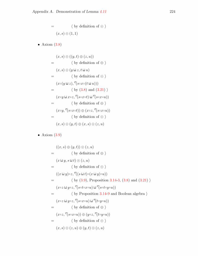
Appendix A. Demonstration of Lemma 4.11 224
= 〈 by definition of � 〉
(x, s)� (1, 1)
• Axiom (3.8)
(x, s)� ((y, t)⊕ (z, u))
= 〈 by definition of ⊕ 〉
(x, s)� (y H z, t H u)
= 〈 by definition of � 〉
(x2(y H z), pp(s2x2(t H u)))
= 〈 by (3.8) and (3.21) 〉
(x2y H x2z, pp(s2x2t) H pp(s2x2u))
= 〈 by definition of ⊕ 〉
(x2y, pp(s2x2t))⊕ (x2z, pp(s2x2u))
= 〈 by definition of � 〉
(x, s)� (y, t)⊕ (x, s)� (z, u)
• Axiom (3.9)
((x, s)⊕ (y, t))� (z, u)
= 〈 by definition of ⊕ 〉
(x H y, s H t)� (z, u)
= 〈 by definition of � 〉
((x H y)2z, pp((s H t)2(x H y)2u))
= 〈 by (3.9), Proposition 3.14-3, (3.8) and (3.21) 〉
(x2z H y2z, pp(s2t2x2u) H pp(s2t2y2u))
= 〈 by Proposition 3.14-9 and Boolean algebra 〉
(x2z H y2z, pp(s2x2u) H pp(t2y2u))
= 〈 by definition of ⊕ 〉
(x2z, pp(s2x2u))⊕ (y2z, pp(t2y2u))
= 〈 by definition of � 〉
(x, s)� (z, u)⊕ (y, t)� (z, u)

Appendix A. Demonstration of Lemma 4.11 225
• Axiom (3.10)
(x, s)~ � (x, s)⊕ (1, 1)
= 〈 by definition of ~ 〉
(x×, pp(x×2s))� (x, s)⊕ (1, 1)
= 〈 by definition of � 〉
(x×2x, pp(pp(x×2s)2x×2s))⊕ (1, 1)
= 〈 by definition of ⊕ 〉
(x×2x H 1, pp(pp(x×2s)2x×2s) H 1)
= 〈 by (3.10), Proposition 3.14-7 and Boolean algebra 〉
(x×, pp(x×2s))
= 〈 by definition of ~ 〉
(x, s)~
Rather than demonstrate (3.12) and (3.13), we work on Laws (3.17) and (3.18)
which are equivalent (see Remark 3.2).
• Law (3.17)
(x, s)� (z, u) E (z, u)
⇐⇒ 〈 by definition of � 〉
(x2z, pp(s2x2u)) E (z, u)
⇐⇒ 〈 by (A.1) 〉
x2z E z ∧ pp(s2x2u) E u
⇐⇒ 〈 by Proposition 3.14-9 and Boolean algebra 〉
x2z E z ∧ s E u ∧ pp(x2u) E u
=⇒ 〈 by (3.17) and (3.22) 〉
x×2z E z ∧ s E u ∧ pp(x×2u) E u
=⇒ 〈 by Proposition 3.14-8 〉
x×2z E z ∧ pp(x×2s) E pp(x×2u) ∧ pp(x×2u) E u
=⇒ 〈 by Boolean algebra and Proposition 3.14-9 〉
x×2z E z ∧ pp(pp(x×2s)2x×2u) E u

Appendix A. Demonstration of Lemma 4.11 226
⇐⇒ 〈 by (A.1) 〉
(x×2z, pp(pp(x×2s)2x×2u)) E (z, u)
⇐⇒ 〈 by definition of � 〉
(x×, pp(x×2s))� (z, u) E (z, u)
⇐⇒ 〈 by definition of ~ 〉
(x, s)~ � (z, u) E (z, u)
• Law (3.18)
(z, u)� (x, s) E (z, u)
⇐⇒ 〈 by definition of � 〉
(z2x, pp(u2z2s)) E (z, u)
⇐⇒ 〈 by (A.1) 〉
z2x E z ∧ pp(u2z2s) E u
⇐⇒ 〈 by Proposition 3.14-9 and Boolean algebra 〉
z2x E z ∧ pp(z2s) E u
=⇒ 〈 by (3.18) 〉
z2x× E z ∧ pp(z2s) E u
⇐⇒ 〈 by Proposition 3.14-8 〉
z2x× E z ∧ pp(z2x×2s) E pp(z2s) ∧ pp(z2s) E u
=⇒ 〈 by (3.20) 〉
z2x× E z ∧ pp(z2pp(x×2s)) E u
⇐⇒ 〈 by Boolean algebra and Proposition 3.14-9 〉
z2x× E z ∧ pp(u2z2pp(x×2s)) E u
⇐⇒ 〈 by (A.1) 〉
(z2x×, pp(u2z2pp(x×2s))) E (z, u)
⇐⇒ 〈 by definition of � 〉
(z, u)� (x×, pp(x×2s)) E (z, u)
⇐⇒ 〈 by definition of ~ 〉
(z, u)� (x, s)~ E (z, u)
The fact that (T,⊕,e, , (1, 1), (>,>)) is a Boolean algebra directly follows from
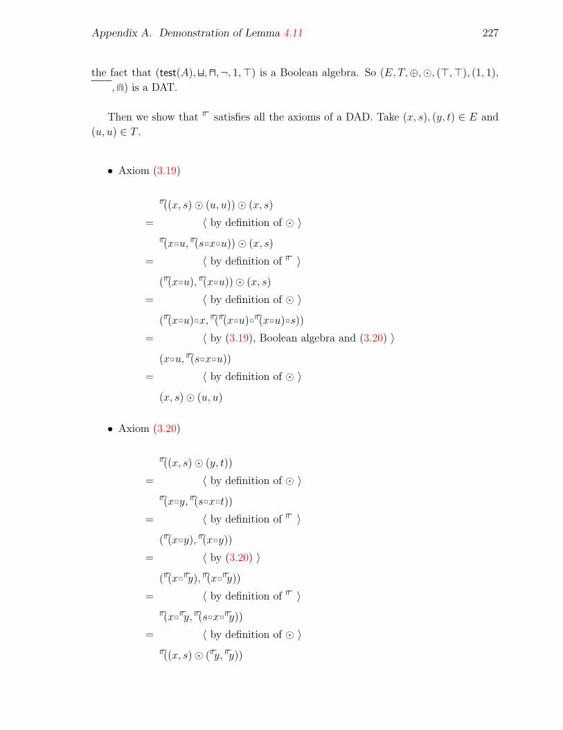
Appendix A. Demonstration of Lemma 4.11 227
the fact that (test(A),H,G,¬, 1,>) is a Boolean algebra. So (E, T,⊕,�, (>,>), (1, 1),
,e) is a DAT.
Then we show that pp satisfies all the axioms of a DAD. Take (x, s), (y, t) ∈ E and
(u, u) ∈ T .
• Axiom (3.19)
pp((x, s)� (u, u))� (x, s)
= 〈 by definition of � 〉
pp(x2u, pp(s2x2u))� (x, s)
= 〈 by definition of pp 〉
(pp(x2u), pp(x2u))� (x, s)
= 〈 by definition of � 〉
(pp(x2u)2x, pp(pp(x2u)2pp(x2u)2s))
= 〈 by (3.19), Boolean algebra and (3.20) 〉
(x2u, pp(s2x2u))
= 〈 by definition of � 〉
(x, s)� (u, u)
• Axiom (3.20)
pp((x, s)� (y, t))
= 〈 by definition of � 〉
pp(x2y, pp(s2x2t))
= 〈 by definition of pp 〉
(pp(x2y), pp(x2y))
= 〈 by (3.20) 〉
(pp(x2ppy), pp(x2ppy))
= 〈 by definition of pp 〉
pp(x2ppy, pp(s2x2ppy))
= 〈 by definition of � 〉
pp((x, s)� (ppy, ppy))

Appendix A. Demonstration of Lemma 4.11 228
= 〈 by definition of pp 〉
pp((x, s)� pp(y, t))
• Axiom (3.21)
pp((x, s)⊕ (y, t))
= 〈 by definition of ⊕ 〉
pp(x H y, s H t)
= 〈 by definition of pp 〉
(pp(x H y), pp(x H y))
= 〈 by (3.21) 〉
(ppx H ppy, ppx H ppy)
= 〈 by definition of ⊕ 〉
(ppx, ppx)⊕ (ppy, ppy)
= 〈 by definition of pp 〉
pp(x, s)⊕ pp(y, t)
• Axiom (3.22)
pp((x, s)� (u, u)) E (u, u)
⇐⇒ 〈 by definition of � 〉
pp(x2u, pp(s2x2u)) E (u, u)
⇐⇒ 〈 by definition of pp 〉
(pp(x2u), pp(x2u)) E (u, u)
⇐⇒ 〈 by (A.1) 〉
pp(x2u) E u
=⇒ 〈 by (3.22) 〉
pp(x×2u) E u
⇐⇒ 〈 by (A.1) 〉
(pp(x×2u), pp(x×2u)) E (u, u)
⇐⇒ 〈 by definition of pp 〉
pp(x×2u, pp(pp(x×2s)2x×2u)) E (u, u)
⇐⇒ 〈 by definition of � 〉
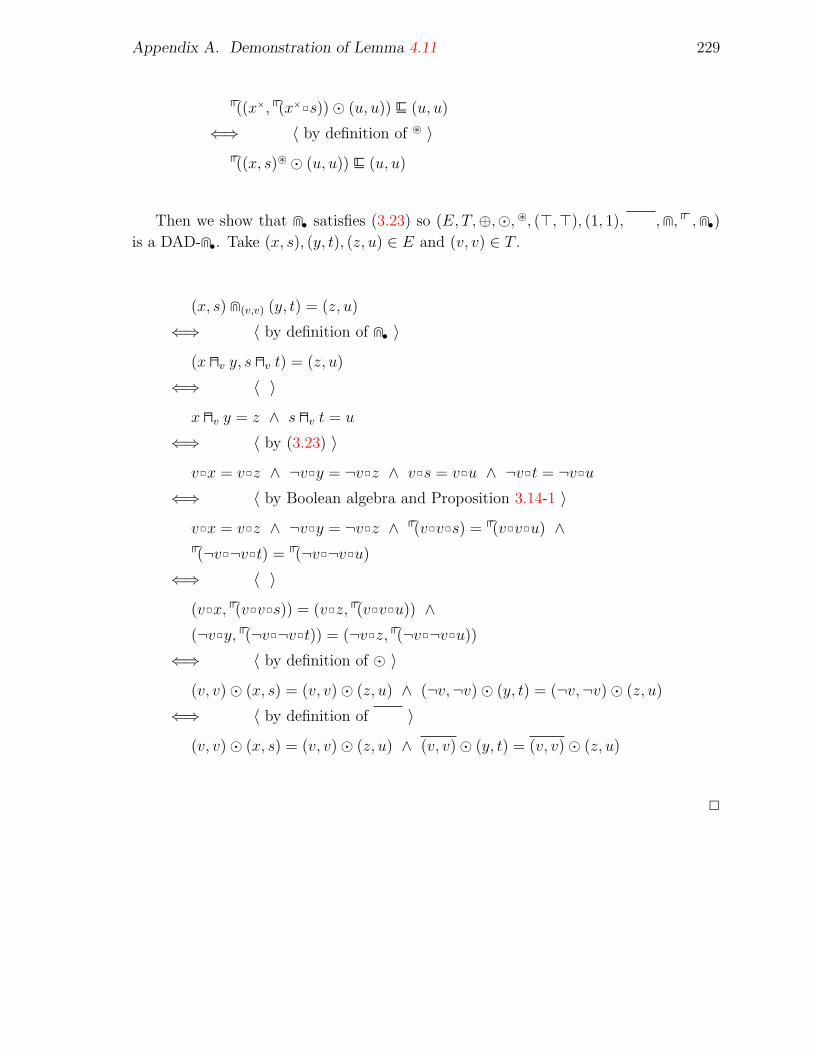
Appendix A. Demonstration of Lemma 4.11 229
pp((x×, pp(x×2s))� (u, u)) E (u, u)
⇐⇒ 〈 by definition of ~ 〉
pp((x, s)~ � (u, u)) E (u, u)
Then we show that e• satisfies (3.23) so (E, T,⊕,�, ~, (>,>), (1, 1), ,e, pp,e•)is a DAD-e•. Take (x, s), (y, t), (z, u) ∈ E and (v, v) ∈ T .
(x, s) e(v,v) (y, t) = (z, u)
⇐⇒ 〈 by definition of e• 〉
(x Gv y, s Gv t) = (z, u)
⇐⇒ 〈 〉
x Gv y = z ∧ s Gv t = u
⇐⇒ 〈 by (3.23) 〉
v2x = v2z ∧ ¬v2y = ¬v2z ∧ v2s = v2u ∧ ¬v2t = ¬v2u
⇐⇒ 〈 by Boolean algebra and Proposition 3.14-1 〉
v2x = v2z ∧ ¬v2y = ¬v2z ∧ pp(v2v2s) = pp(v2v2u) ∧pp(¬v2¬v2t) = pp(¬v2¬v2u)
⇐⇒ 〈 〉
(v2x, pp(v2v2s)) = (v2z, pp(v2v2u)) ∧(¬v2y, pp(¬v2¬v2t)) = (¬v2z, pp(¬v2¬v2u))
⇐⇒ 〈 by definition of � 〉
(v, v)� (x, s) = (v, v)� (z, u) ∧ (¬v,¬v)� (y, t) = (¬v,¬v)� (z, u)
⇐⇒ 〈 by definition of 〉
(v, v)� (x, s) = (v, v)� (z, u) ∧ (v, v)� (y, t) = (v, v)� (z, u)
2
Index
t-conditional operator, 26, 55
Algebra of decomposable elements, 85
Angelic choice, 75, 77
Angelic composition, 79, 86
Angelic iteration operator, 90
Angelic refinement, 75
Codomain operator, 79
Competence set, 204
DA, see Demonic algebra (DA)
DAD, see Demonic algebra with domain
(DAD)
DAD-G•, see Demonic algebra with do-
main and t-conditional
(DAD-G•)
DAT, see Demonic algebra with tests
(DAT)
Decomposition, 79, 80
Demonic algebra (DA), 34
Demonic algebra with domain (DAD),
42
Demonic algebra with domain and
t-conditional (DAD-G•), 54, 55
Demonic algebra with tests (DAT), 38,
39
Demonic composition, 20
Demonic iteration operator, 21
Demonic join, 19
Demonic refinement, 19
Demonic refinement algebra (DRA), 4,
207
Demonic refinement algebra with
enabledness (DRAe), 5, 208
Disjoint, 39
Divergence operator, 206
Domain operator, 16, 42
DRA, see Demonic refinement algebra
(DRA)
DRAe, see Demonic refinement algebra
with enabledness (DRAe)
Enabledness operator, 208
Guard, 208
KA, see Kleene algebra (KA)
KA-implication, 18
KAD, see Kleene algebra with domain
(KAD)
KAT, see Kleene algebra with tests
(KAT)
Kleene algebra (KA), 3, 12, 13
Kleene algebra with domain (KAD), 16
Kleene algebra with tests (KAT), 14, 15
Left annihilator, 46
Left preserver, 46
Locality, 16, 43
Maximal subalgebra of decomposable
elements, 85
Positively conjunctive, 4, 206
Predicate transformer, 3, 206
Probabilistic choice operator, 214
RA, see Relation algebra (RA)
Relation algebra (RA), 2
Zorn’s Lemma, 85