Demand Response Plan Considering Available

Spinning Reserve for System Frequency Restoration Le-Ren Chang-Chien, Member, IEEE, Luu Ngoc An, Ta-Wei Lin

Abstract-In the proposed frequency restoration plan, demand response is adopted as the first shedding option for intercepting frequency decline in order to avoid the unexpected load shedding, then followed by the scheduled generation reserve to raise frequency back to the normal state. This paper starts with the frequency response analysis using a low-order frequency response model. Results of the frequency response analysis show that, if the magnitude of system disturbance is accurately estimated following the moment of incident, the estimate could be intelli­gently used to deploy appropriate demand response for frequency restoration. Tests of the proposed frequency restoration scheme are evaluated by simulation where the system data is utilized by records of historical frequency events from a utility. Test results show that the deployment of the demand response could enhance frequency security under various contingency scenarios.

Index Terms-Demand response, under frequency load shed­ding, load-frequency control

I. INTRODUCTION

WHEN an electric power system encounters a serious

network disturbance or a large unit trip, system fre­

quency would drop substantially and result in malfunction

of the network equipment. If the frequency decline is not

effectively stopped in a short period of time, cascading events

of network failure could further cause a blackout. To avoid

the declined frequency that may cause cascading outages, a

decisive frequency control using the spinning reserve or load

shedding is essential. In most power systems, the Under­

Frequency Load Shedding (UFLS) is considered as the last

defense line to save system frequency. How the shedding load

is applied to save the endangered system frequency has been

widely discussed in literatures. The conventional UFLS is

designed by monitoring the frequency as an incident index

for decision making [1,2]. When the system frequency falls

below a predefined threshold, portions of the system load will

be shed in a few steps. Although this type of UFLS is simple

and easy to be implemented, system operators feel that this

scheme has more room to be improved. The major issue of

this scheme is its lack of adaptability. Since the amount of

the disturbance is unknown. The UFLS scheme is prone to

the preset assumption. Its lack of adaptability may result in

either over-shedding or under-shedding in different situations.

The other approach to avoid this shortcoming is to use the

frequency decline rate as an index to measure the disturbance

This work was performed under research contracts from Taiwan Power Company under grant: TPC 546-2101-9801. and National Science Council under grants: NSC 100-2628-E-006-016, NSC 98-2918-1-006-006-.

Le-Ren Chang-Chien is, Luu Ngoc An and Ta-Wei Lin were with Na­tional Cheng Kung University, No. 1 University Rd. , Tainan, Taiwan.(E-mail: leren@ee. ncku.edu. tw)

magnitude [2,3]. Using this information, more accurate load

could be shed for avoiding the aforementioned drawback.

However, the efficacy of this method is dependent upon the

accuracy of the rate of frequency change. This method could

not perform its prime advantage due to the slow sampling

rate of the old SCADA system until the latest introduction of

the frequency estimation from the Phasor Measurement Unit

(PMU) [4].

With the fast sampling nature of PMU, accurate disturbance

estimation becomes feasible. UFLS could be situated in a

better position by knowing how much load is required to be

shed for balancing the generation loss. However, shedding the

customer load is still risky because the practical shedding

amount is not exactly the same as what operators expect.

Therefore, in the real practice, operators prefer to shed more

load than the estimated value. It may make the following

frequency restoration process more complex [5].

Demand Response (DR) refers to actions initiated from

contracted customers by changing their consumption (demand)

of electric power in response to price signals, incentives, or

directions from grid operators. Emergency Demand Response

(EDR) program is one of the incentive-based demand response

alternatives to provide direct load control, capacity, and ancil­

lary service during the real-time [6]. If EDR is utilized in the

UFLS, blocks of EDR selection would make the tripping of

load more accurate. System operators would be more confident

of the frequency response following the UFLS. Incorporating

DR to deal with frequency events is not new, however, how to

execute appropriate DR to achieve the responsive and smooth

frequency restoration is the issue in need of more investigation.

II. ESTIMATION ON THE MAGNITUDE OF SYSTEM

DISTURBANCE

A. System Frequency Response Model

System frequency is the only observable index that indicates

the extent of power imbalance within the system. It goes

without saying that the nature of system frequency is a clue

to estimate the magnitude of system disturbance. To study

the nature of system frequency after the disturbance, we shall

begin with the review of system frequency response model [7].

The System Frequency Response (SFR) model is a simpli­

fied frequency model used in a real-time for predicting the

frequency behavior of a large scale power system subjecting

to a disturbance. The basic concept of the model derived here

is based on the idea of uniform or averaged frequency, where

synchronizing oscillations between generators are filtered out,

978-1-4673-2868-5/12/$31.00 ©2012 IEEE

2

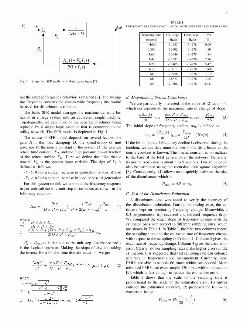
TABLE I Pd +

�I 1 /).0) FREQUENCY RESPONSE CALCULATION WITH DIFFERENT SAMPLING RATES

2Hs+D - � P a

P m

Km (1 + FHTRs) R(I + TRs)

Fig. 1. Simplified SFR model with disturbance input [7].

but the average frequency behavior is retained [7]. The averag­

ing frequency presents the system-wide frequency that would

be used for disturbance estimation.

The basic SFR model averages the machine dynamic be­

havior in a large system into an equivalent single machine.

Topologically, we can think of the separate machines being

replaced by a single large machine that is connected to the

utility network. The SFR model is depicted in Fig. 1.

The nature of SFR model depends on several factors: the

gain Km, the load damping D, the speed-droop of unit

governor R, the inertia constant of the system H, the average

reheat time constant TR, and the high pressure power fraction

of the reheat turbine F H. Here we define the "disturbance

power" Pd as the system input variable. The sign of Pd is

defined as follows:

-Pd > 0 For a sudden increase in generation or loss of load

-Pd < 0 For a sudden increase in load or loss of generation

For this system model, we compute the frequency response

in per unit subject to a unit step disturbance, as shown in the

following equation,

� ( Rw;

) ( 1 + TR8

) Pstep (1)

W = D x R + Km 82 + 2(Wn8 + W� 8

where 2 _ D x R+Km Wn - 2H x R x TR

( _ (2H x R + (D x R + Km x FH) X TR) - 2(D x R+Km) Wn

Pd = Pstep/8 is denoted as the unit step disturbance and s

is the Laplace operator. Making the slope of �w and taking

the inverse form for the time domain equation, we get

(2)

Sampling time Est. slope Exact slope Error

(second) (Hz/s) (Hz/s) (%) 111000 -3.4247 -3.4278 0. 09

11100 -3.3902 -3.4278 1. 10

1/60 -3.3649 -3.4278 1. 84

1/40 -3.3333 -3.4278 2. 76

1120 -3.2405 -3.4278 5. 47

1110 -3.0617 -3.4278 10. 68

1/8 -2.9758 -3.4278 13. 19

1/6 -2.8373 -3.4278 17. 23

115 -2.7308 -3.4278 20. 34

B. Magnitude of System Disturbance

We are particularly interested in the value of (2) at t = 0, which corresponds to the maximum rate of change of slope

d�w(t) I =

awnR x pstep . =

Pstep (3)

dt t=O D x R+ Km

Slllipl 2H

The initial slope of frequency decline, mo, is defined as

m = d�w(t)

I = Pstep

(HZ/8) (4) o dt t=O 2H

If the initial slope of frequency decline is observed during the

incident, we can determine the size of the disturbance as the

inertia constant is known. The inertia constant is normalized

to the base of the total generation in the network. Generally,

its normalized value is about 3 to 5 seconds. This value could

also be estimated using the recursive least square algorithm

[8]. Consequently, (4) allows us to quickly estimate the size

of the disturbance, which is

Pstep = 2H x mo (5)

C. Test of the Disturbance Estimation

A disturbance case was tested to verify the accuracy of

the disturbance estimation. During the testing case, the es­

timator kept on monitoring frequency change. Meanwhile, a

0.4 pu generation trip occurred and induced frequency drop.

We compared the exact slope of frequency change with the

estimated ones with respect to different sampling rates, which

are shown in Table I. In Table I, the first two columns record

the sampling time and the estimated rate of frequency change

with respect to the sampling in Column 1. Column 3 gives the

exact rate of frequency change. Column 4 gives the estimation

error. Clearly, slower sampling rates make higher errors in the

estimation. It is suggested that fast sampling rate can enhance

accuracy in frequency slope measurement. Currently, most

PMUs are able to sample 60 times within one second. More

advanced PMUs can even sample 120 times within one second

[9], which is fast enough to reduce the estimation error.

Table I shows that the scale of the sampling time is

proportional to the scale of the estimation error. To further

enhance the estimation accuracy, [2] proposed the following

correction factor.

mO 2 Pstep = H ( 30 +

r s ) (6)

4.5

3.5 3

2.5

1.5

1

0.5 o

V.Lp"

.0.41'''

.0.61''' -

-

- -

- - -

- - -\

-=-- - -

- - -r- -r- -,-- � 1/1000 1/100 1/60 1/40 1/20 1/10 1/8 1/6 1/5

•• mpling tlmal.acl

Fig. 2. Pstep error vs. different sampling with respect to various disturbance magnitudes

where

Pstep estimated system disturbance (pu)

H system inertial constant (s)

mo estimated slope (Hz/s)

T s sampling rate (sample/s) Based on (6), we can deduce that the corrected slope mo',

is as follows. , 60 mo = mo + - Hz/s

Ts (7)

(6) is proven to work well in large systems when frequency

decline is not too steep. However, we also found that the

correction is not sensitive to the slope of frequency change,

mo, i.e., the disturbance magnitude, which may also affect

the accuracy of the estimation error. Therefore, we propose

another correction factor to take care of this effect.

, mo mnew = mo + - Hz/s

Ts

Therefore, (6) becomes

mnew' Pstep = 2H ( ----w-) Hz/s

(8)

(9)

After using the correction in (9), Fig. 2 shows the estimation

error vs. different sampling with respect to various disturbance

magnitudes. The result indicates that the proposed correction

factor not only effectively reduces the estimation error (com­

pared to Table I) but also reduces the correction uncertainty

that is affected by different disturbance magnitudes.

III. DESIGN OF THE FREQUENCY RES TORATION

PLAN CONSIDERING DEMAND RESPONSE AND

SPINNING RESERVE

A. Incorporate Direct Load Control Demand Response into

the Load Shedding Plan

Direct load control demand response can serve as the reserve

capacity for dealing with the frequency events. Shutting down

the contracted load (including pumped storage units as they are

operating in pumping mode) helps system frequency returning

quickly to the acceptable level following the loss of mass

generation. However, over-shedding of demand response may

make frequency suddenly go beyond the nominal level and

result in frequency oscillation, which makes the subsequent

frequency restoration process more complicated. Therefore,

how to appropriately allocate demand response to rescue the

endangered frequency and then facilitate frequency restoration

process is the issue in need of more attention.

B. Under Frequency Load Shedding Plan of a Utility

In a utility of our study case, the range of continuous

operating frequency is between 59.7, and 60.3Hz. To account

for the rate of change of frequency effect, and avoid possible

vibration and resonance occurring in some units' turbines, the

first stage of load-shedding frequency is set at 59. 5Hz with a

50 second time delay. If the first stage load-shedding is not

sufficient for stopping the descending frequency, the second

stage of under-frequency relay will be initiated immediately to

shed customer load when the frequency drop to 59.2Hz [5]. In

order not to shed the undesired customer load when frequency

reaches 59.2Hz, Emergency Demand Response (EDR) plan

is designed according to this defense line. In our design

strategy, EDR is divided into two parts. The first part, EDRI,

is allocated to prevent the 59.2Hz load shedding. The second

part, EDR2, is designed to bring the declined frequency back

to a secure level at 59.7Hz so that spinning reserve could carry

on the restoration afterwards.

C. Determine the EDR and spinning reserve for Contingency

Planning

To deploy sufficient demand response for frequency secu­

rity, we calculate the least quantity of the demand response

(EDRl) for the maximum single contingency (Pmax) scenario.

Assuming that the EDRI is planned to save the descending

frequency from the 59.2Hz frequency level, the required least

quantity of EDRI is equal to the following relation,

EDRI = Pmax - Pjmin (lO)

where Pmax is defined as the MW single contingency, Pjmin is the deficit MW power that makes frequency drop from

nominal frequency (fo) to minimum frequency (fmin). In our

study case, (fo) and imin are 60Hz and 59. 2Hz, respectively.

From ( 1), the deficit MW power Pjmin can be calculated

as follows,

P min = (fo - imin) (D X

.R + Km)

j Rx (l+ae-(Wntzslllwrtz+'P)

(1 1)

where tz is the time duration of frequency decline when

frequency reaches imino tz can be calculated as follows.

n7r - 'PI 1 WrTR tz = = - arctan( ) (12)

Wr Wr (wrTR - 1 Once EDRI is determined by the planning procedure, the

remaining EDR would be allocated as EDR2 whose mission

is to bring the declined frequency up to a secure level (59.7

Hz). It is noted that EDR2 can be coordinated with available

Fast Spinning Reserves (FSR) to fulfill this task. The required

per unit amount of EDR2 and FSR is calculated as follows.

EDR2 + FSR = 6.Pmax - EDRI _ (60 - 59.7)

(D + �) 60 (fj)

After restoring frequency back to 59.7 Hz, the least remain­

ing reserve, which is called Slow Spinning Reserve (SSR), to

be planned for continuously returning frequency back to 60Hz

is calculated as follows.

SSR = 6.Pmax - (EDRI + EDR2 + FSR) (14)

Units participating SSR could be slower response spinning

units, or fast start turbines.

IV. EXECUTION OF THE PROPOSED FREQUENCY

RESTORATION SCHEME

If the magnitude of system disturbance is quickly estimated,

appropriate EDR could be executed to bring the declined fre­

quency back to the expected level. Once EDRI is determined

by the planning procedure, the remaining demand response

would be allocated as EDR2 to bring back the frequency up

to a secure level. Detail of the EDR execution procedure is

described as follows.

A. Determine the disturbance magnitude

When a sudden frequency drop is detected by the PMU,

the system control center would instantly calculate initial rate

of the frequency decline, this value is used to calculate the

magnitude of system disturbance (Pstep) as of (9).

B. Decision making for triggering EDR1 or EDR2

1) Moment of EDR1 execution: Once Pstep is obtained,

Pstep is compared with Pjmin. If Pstep > Pjmin , it means

the contingency amount could drag frequency below f min (59.2Hz). Therefore, EDRI is initiated. Otherwise, the step is

passed to option B. After the execution of EDRl, the renewed

power deficit is calculated using the following equation,

Prenew = Pstep - ED Rl (15)

2) Moment of EDR2 execution: In this option, the cor­

responding MW power difference (Pjmin2) between the

frequency fa and fmin2 is calculated. The calculation of

(Pjmin2) is the same as ( 11) where the fmin is replaced by

fmin2. In our study case, fmin2 is chosen at 59.7Hz, which is

considered as a secure level so that spinning reserve could have

enough time to react for frequency restoration. Once Pjmin2 is obtained, the MW power that EDR2 is going to be casted

in the system is equal to the following relation if option 1 is

not executed.

Ps1ep>P fmin

(fmin =59.2H�

False

f <59.7Hz

fss <59.5Hz

False

True

False After 50s, shed load

I END I

Fig. 3. Schematic of the EDR control for frequency events.

4

V. TEST OF THE EMERGENT DEMAND RESPONSE SCHEME

In this paper, the adaptive EDR control scheme is tested.

Our primary goal is to use EDRI as the first shedding step

to avoid shedding unwanted customer loads at 59.2Hz. Our

secondary goal is to allocate sufficient EDR2 so that frequency

could be quickly brought back to a secure level (59.7Hz).

In order to prove that the EDR plan can fit into various

contingency scenarios, we make some tests with different

scales of disturbances which were taken by real data sampled

from a utility. The simulation will evaluate the performance

of the EDR scheme.

EDR2 = Pstep - Pjmin2 (16) A. System Modeling for the Contingency Test

otherwise

EDR2 = Prenew - Pjmin2 (17)

Using the above relation, more accurate amount of EDR2

will be allocated for restoring the frequency back to the

expected level.

Note that if EDRI is not utilized in the option A,

EDRI would be then automatically allocated for EDR2. The

schematic of the EDR control is depicted in Fig. 3.

In order to closely simulate the frequency event of a utility,

system parameters used in the simulation must be accurate

enough to reflect the real frequency trend. The parameters are

estimated by the following way: first, collecting the system

parameters (such as system droop, load damping, and inertia,

etc) and historical frequency response from a utility. After

that, we try to make the frequency response of the SFR model

as close as possible to the historical record. The estimated

parameters are then confirmed to be used for simulations.

N I

60

59.8

� 59.6

� � 59.4 E El � (/) 59.2

59

�

f VI 1/ V

� � "- .

-----

resel ,e

� �

"--. !,----, ,;th" C,R1

�itt 10Llt EDR

58.8 o 50 100 150 200

Time (sec) 250 300 350

Fig. 4. Simulated frequency curves of scenario I.

B. Scenario 1: The most severe disturbance

400

In this scenario, the utility is assumed to have 500MW de­

mand response. When the power system is operating at 25000

MW demand, a maximum single contingency (1900MW)

disturbance occurs at f = 60 Hz. The estimated minimum

system frequency value would be below 59 Hz.

According to ( 10), the amount of EDRI was planned to

deal with the maximum single contingency in the system

is 472.5MW. As a result, the 500MW demand response is

allocated as EDRI. The frequency response curves are shown

in Fig. 4 and the decision process of the EDR is shown in Fig.

5.

Fig. 4 shows that when a disturbance occurs without the

support of EDR1, the frequency could be down below 59.2 Hz.

When the frequency drops below 59.7Hz, EDR1 is initiated.

After using the EDRl, the frequency dip is raised above 59.2

Hz and then settled above 59.5Hz. Following the response of

EDR1, the spinning reserve continues to restore the frequency

back to 60 Hz within 5 minutes.

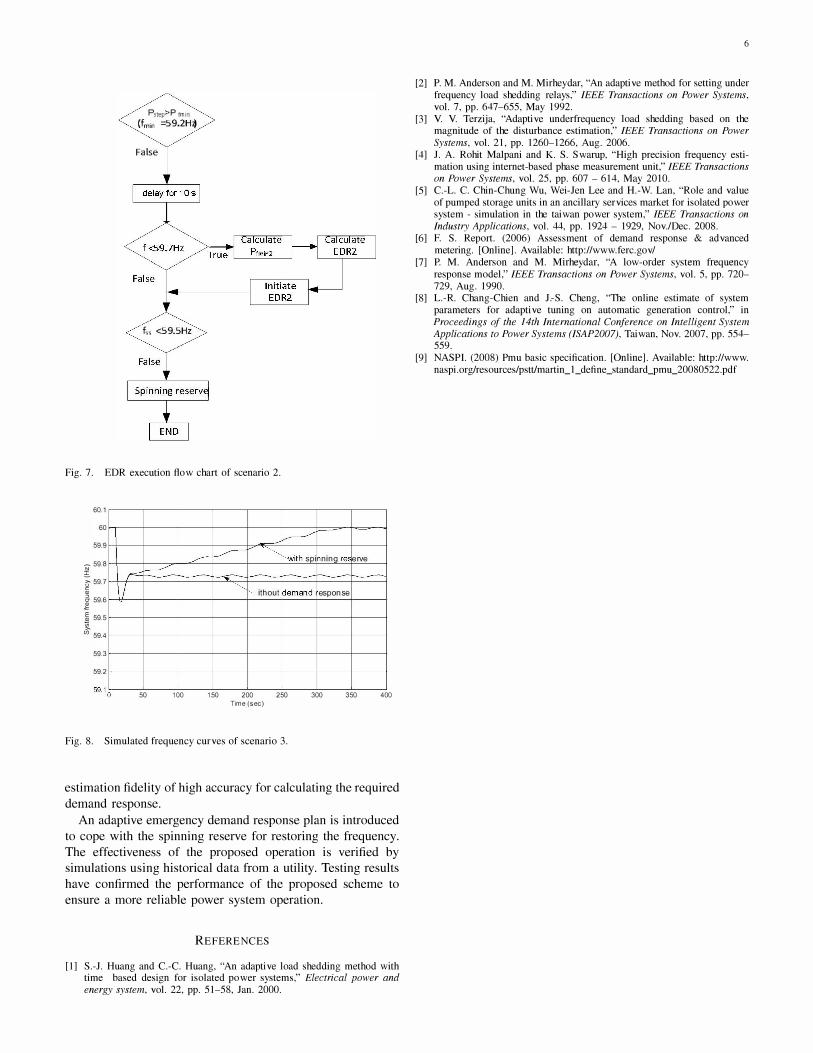
C. Scenario 2: Medium disturbance

In this scenario, it is assumed that the system has 500MW

demand response. When the power system is operating at

20200 MW demand, a single contingency ( 1 100MW) distur­

bance occurs at f = 60 Hz.

Because the amount of the disturbance is not large enough

to make the frequency decline below 59.2Hz, it does not

need to initiate EDRI. Following that, the execution process

is passed to option 2. According to (13), 500MW EDR2 is

sufficient to raise frequency up to 59.7 Hz secure level. After

the activation of EDR2, spinning reserve follows to restore the

frequency back to 60Hz. Simulated frequency curves and the

EDR execution process are shown in Fig. 6 and 7.

D. Scenario 3: Small disturbance

In this scenario, it is assumed that the system has 500MW

demand response. When the power system is operating at

2 1500 MW demand, a single contingency (650MW) unit trip

occurs at f = 60 Hz. Because the amount of disturbance is

small, the estimated steady state frequency drop is still above

Pstep>Pfmin (f m;n =59.2H2)

False

f<59.7Hz

False

f" <59.5Hz

Fig. 5. EDR execution flow chart of scenario 1.

60. 1

60

59.9

N 59.8

I � 59.7 " 5- 59.6 & � 59.5 � (/) 59.4

59.3

59.2

59. 1

� V

� -----

/ /!'-I '",",

II V

� f-----

"'--v ith spinn ng reser e

"'-with DR2-5C pMW

without �emand esponse

50 100 150 200 Time (sec)

250 300 350 400

Fig. 6. Simulated frequency curves of scenario 2.

59.7 Hz. Thus, we just need to use the spinning reserve to

restore the frequency back to 60 Hz. The frequency curves

are shown in Fig. 8.

VI. CONCLUSION

For frequency security concern, power system operation

should be able to perform high reliability by means of auto­

matic control when the system encounters contingent events.

Therefore, how to design and execute a suitable frequency

restoration plan for the power system has become an important

topic. This paper proposes a new adaptive demand response

scheme to achieve this goal.

A linear system frequency response (SFR) model is adopted

to calculate the amount of system disturbance by means of

measuring the system frequency through PMU. Surveys of

the estimated magnitude of the disturbance have proven the

Pstep>Prmin (fmin =59.2H;)

False

f" <59.5Hz

Fig. 7. EDR execution flow chart of scenario 2.

60.1 60

59.9 N 59.8 I i 59.7 � 159.6 � 59.5 � (f) 59.4

59.3 59.2

,-=:.

.I

� V-- � �

� without

� t'-with spi ning re, elVe

� emand esponse

50 100 150 200 Time (sec)

250 300 350

Fig. 8. Simulated frequency curves of scenario 3.

400

estimation fidelity of high accuracy for calculating the required

demand response.

An adaptive emergency demand response plan is introduced

to cope with the spinning reserve for restoring the frequency.

The effectiveness of the proposed operation is verified by

simulations using historical data from a utility. Testing results

have confirmed the performance of the proposed scheme to

ensure a more reliable power system operation.

REFERENCES

[1] S. -J. Huang and c.-c. Huang, "An adaptive load shedding method with time based design for isolated power systems," Electrical power and

energy system, vol. 22, pp. 51-58, Jan. 2000.

[2]

[3]

[4]

[5]

[6]

[7]

[8]

[9]

6

P. M. Anderson and M. Mirheydar, "An adaptive method for setting under frequency load shedding relays," IEEE Transactions on Power Systems, vol. 7, pp. 647-655, May 1992. Y. Y. Terzija, "Adaptive underfrequency load shedding based on the magnitude of the disturbance estimation," IEEE Transactions on Power

Systems, vol. 21, pp. 1260-1266, Aug. 2006. J. A. Rohit Malpani and K. S. Swarup, "High precision frequency esti­mation using internet-based phase measurement unit," IEEE Transactions on Power Systems, vol. 25, pp. 607 - 614, May 2010. c.-L. C. Chin-Chung Wu, Wei-Jen Lee and H. -W. Lan, "Role and value of pumped storage units in an anciUary services market for isolated power system - simulation in the taiwan power system," IEEE Transactions on

Industry Applications, vol. 44, pp. 1924 - 1929, Nov. lDec. 2008. E S. Report. (2006) Assessment of demand response & advanced metering. [Online]. Available: http://www. ferc. gov/ P. M. Anderson and M. Mirheydar, "A low-order system frequency response model," IEEE Transactions on Power Systems, vol. 5, pp. 720-729, Aug. 1990. L. -R. Chang-Chien and J.-S. Cheng, "The online estimate of system parameters for adaptive tuning on automatic generation control," in Proceedings of the 14th International Conference on Intelligent System Applications to Power Systems (lSAP2007), Taiwan, Nov. 2007, pp. 554-559. NASPI. (2008) Pmu basic specification. [Online]. Available: http://www. naspi. orgiresources/pstUmartin_l_ define _standard_pm u_200805 22. pdf