1

Considering Potential Bias in Macro-estimates of the Elasticity of Labour Demand

Jussi Huuskonen

December 30, 2016

Bacground report for the Economic Policy Council

1 INTRODUCTION

The Finnish government’s competitiveness pact is the key measure by which it aims to raise employment. The objective is to improve cost-competitiveness by lowering labour costs in the private sector, thereby increasing employment. The Ministry of Finance (MoF) estimates (1.3.2016) that the competitiveness pact will reduce unit labour costs by 4.2% compared to the baseline scenario. Ac-cording to the MoF, this will improve employment by approximately 35,000 persons compared to the baseline scenario by the beginning of the 2020s. The elasticity of labour demand plays a key role in assessing the employment impacts of the competitiveness pact. Therefore, the elasticity estimate used should be as accurate and reliable as possible. The elasticity of labour demand reflects how responsive labour demand is to changes in labour costs. A point estimate for the elasticity of labour demand indicates the percentage increase in labour demand if labor costs are reduced by 1%. The MoF (29.9.2015) uses an elasticity estimate of -0.7 for the private sector. The idea of this background report is based on the latest Economic Policy Council Report (2016, p. 86-91), which argued that the government’s estimate for labour demand elasticity is very high and predicts overly optimistic em-ployment effects. The majority of studies estimate demand elasticities using ag-gregate data. Such studies lack exogenous variation in labour costs, which makes it impossible to measure the causal impacts of labour costs on employ-ment in a reliable way. Lichter et al. (2014) provide an extensive survey of the empirical literature relat-ed to the own-wage elasticity of labour demand. They conduct a meta-regression analysis to re-assess empirical studies of labour demand elasticities. Their analysis is based on 924 elasticity estimates obtained from 105 studies. The sample comprises estimates from studies for 37 countries published be-tween 1980 and 2012. The overall mean own-wage elasticity of labour demand in their sample is -0.51, with a standard deviation of 0.77. On the basis of these estimates, the MoF’s elasticity of -0.7 does not seem impossibly high. However, Lichter et al. (2014) claim that many estimates of the own-wage elasticity of la-

2

bour demand given in the literature are unreasonably high and upwardly in-flated, and their preferred estimate of constant output elasticity is -0.25. Estimating labour demand elasticities based on macro-data is likely to produce biased and unreliable estimates. The problems relate in particular to i) the lack of exogenous variation in labour costs, ii) the simultaneity of demand and sup-ply, and iii) the possibility of composition bias. Using aggregate data in estimat-ing labour demand elasticities is problematic since such data lack exogenous variation in labour costs. Wages and employment are both endogenous varia-bles, which constitutes a problem. When the purpose is to make policy analysis and predict the effects of reducing labour costs, it is necessary to have exoge-nous variation in labour costs. Macro-models also ignore the simultaneity of demand and supply. This report shows that the estimates used in calculating the employment effects of the competitiveness pact are likely to be severely upward-biased. The empir-ical analysis in this report estimates labour demand elasticities using different wage variables. Since the same model and the same time period are used for every wage variable, the differences between elasticities provide evidence of potential bias. A relevant elasticity estimate should be based on research con-taining plausibly exogenous variation in wages. For that reason this report con-tains a small meta-analysis of micro-studies examining situations where labour costs have been altered exogenously.

2 DATA

When estimating the own-wage elasticity of labour demand, employment is the dependent variable and labour costs the independent variable. In addition to these, an estimation equation may also include output as a control variable. The calculations in this report are based on industry-level data. Twenty-six indus-tries are considered, based on the Standard Industrial Classification (TOL2008). Some industries are combined in order to verify the comparability of the data and results. All the data cover the years 1996–2013, while some data are availa-ble since 1975. Data about working hours are used as the measure of employment. The annual data on hours worked in corporations by industry (1975-2015) are obtained from Statistics Finland's Annual national accounts. Output by industry at basic prices using year 2010 prices is obtained from the same source. The panel data on total labour compensation (W) by industry in 1975-2014 is obtained from Sta-tistics Finland's Productivity surveys. This annual private sector data are in nominal form, and are therefore converted into real form using the Producer price index for manufactured products, the base year being 1949. The real wage

3

variable W/L is formed by dividing total labour compensation W by the num-ber of hours worked (L) in each industry for each year. Since the preferred wage variables are available only as changes, W/L is con-verted into Δ(W/L), which represents wage changes. This logarithmic percent-age change in real wages is calculated using natural logarithms and the follow-ing formula:

𝛥(𝑊/𝐿)𝑡 = 𝑙𝑛((𝑊/𝐿)𝑡

(𝑊/𝐿)𝑡−1 ) = 𝑙𝑛(𝑊/𝐿)𝑡 − 𝑙𝑛(𝑊/𝐿)𝑡−1

TABLE 1 Summary of the data Variable Label Obs Mean Std. Dev. Min Max

W Total labour compensation by industry, 1,000,000 €

468 2310.84 2418.366 173 12 305

L Total working hours by industry, 1,000,000 h

468 87.81 96.00 8.2 489.7

Y Total output by industry (2010 prices), 1,000,000 €

468 8412.34 6819.10 817 31 301

P Producer price index 468 0.888 0.069 0.796 1.013

W/L "Real wage" by industry 468 30.190 7.091 16.815 59.462

ΔL Logarithmic % changes in working hours

442 0.0028 0.0526 -0.237 0.204

ΔY Logarithmic % changes in output

442 0.0200 0.0817 -0.324 0.332

Δ(W/L) Logarithmic % changes in “real wage”

442 0.0196 0.0448 -0.110 0.317

RAGR Real aggregate wage growth

468 0.0323 0.0401 -0.189 0.387

RWHR Real wage growth of job stayers

468 0.0312 0.0372 -0.199 0.343

When estimating the own-wage elasticity of labour demand, the dependent var-iable is working hours, which represents employment. The wage variable is used as an independent variable. Since the working hour variable is also a com-ponent of the wage variable Δ(W/L), there will inevitably be some bias in the elasticity estimates. In many studies, however, earnings are simply summed and divided by worker-hours to yield the wage rate. Hamermesh (1996) ques-tions studies that take published aggregates and analyse elasticities for them. In his opinion any such study will generate biased elasticity estimates in equations relating worker-hours to real wages. Hamermesh (1996, 60-71) criticizes estimates of parameters describing employ-ers’ labour demand. He points out that there should be enough exogenous vari-ation in factor prices to allow one to infer the demand elasticities of interest. There should be exogenous variation in wage data or working hours. The sim-ultaneity of demand and supply should also be taken into account. This is be-cause the supply of labour is generally neither perfectly elastic nor inelastic.

4

Consequently, estimating elasticities without a complete system including sup-ply is unsatisfactory. In order to demonstrate the significance of the bias in labour demand elasticities, it is important to find a valid measure for the price of labour. The panel data on the wage variables AGR and WHR is obtained from Mika Maliranta, and the calculation methods are described in Kauhanen and Maliranta (2012). They study the dynamics of the standard aggregate wage growth in macro statistics using micro data, focusing on how job and worker restructuring influence ag-gregate wage growth and its cyclicality. Using comprehensive longitudinal em-ployer–employee data, they measure the growth rate of average wages (the standard aggregate growth rate, AGR) and the average wage growth rate of job stayers (WHR). These data cover the years 1996–2013, and the 26 industries are based on the Standard Industrial Classification (TOL2008). The original wage data were ob-tained from the Confederation of Finnish Industries (EK), being based on an annual survey of employers which forms the basis of the private sector wage structure data maintained by Statistics Finland. The data include detailed in-formation on wages, job titles, and unique person and firm identifiers and form a linked employer–employee panel that allows people to be followed over time (Kauhanen & Maliranta 2012). Since AGR and WHR are originally in nominal form, they are converted into real form so that the estimation results are comparable to the previous real wage data. The conversion is performed using the producer price index for manufactured products.

RAGR = AGR + ln ( 𝑃𝑡−1

𝑃𝑡 )

The aggregate growth rate (AGR) is based on Statistics Finland’s wage structure statistics. AGR measures the growth rate of average wages by industry, and us-ing it instead of the original wage variable Δ(W/L) corrects a major problem in the elasticity estimates. The cause of the problem is that working hours are sim-ultaneously both dependent variable but also a component of the wage variable. Using the independent wage variable RAGR is a step towards more reasonable elasticity estimates. Even if using the real aggregate growth rate RAGR as a wage variable is less prone to produce biased elasticity estimates than Δ(W/L), there might still be composition bias. When using aggregate wage data, the hour shares of different groups vary with business cycles. The work hours of low-wage groups tend to be more cyclically variable than those of high-wage groups. Thus aggregate wage statistics give more weight to low-wage workers during expansions than during recessions. This composition effect biases aggregate wage statistics in a

5

countercyclical direction and is likely to obscure the real wage procyclicality that a typical worker in any group really faces (Solon et al 1994). If aggregate wage statistics are biased due to composition bias, there is reason to believe that elasticity estimates based on such data are also biased. Since the source of the problem is cyclically shifting weights, the most direct solution is to construct a wage statistic without cyclically shifting weights. By following the exact same workers over time, one can keep the composition constant, which results in a wage statistic without cyclically shifting weights (Hamermesh 1986). Comparing the elasticity estimates provides information on the importance and magnitude of the composition bias. The wage growth measure WHR represents the nominal change in hourly wag-es for people who continue in the same firm. Kauhanen and Maliranta (2012) decompose aggregate wage growth into the wage growth of job stayers and job and worker restructuring. A job stayer is an employee who stays in the same firm for two consecutive years. Such calculations of WHR allow for change of profession because the profession data were not available on an annual basis before 2004. Since the composition remains the same, this average wage growth rate of job stayers is free of composition bias. Kauhanen & Maliranta (2012) find that the aggregate wage growth rate is lower than the wage growth rate of job stayers, so the wages of job stayers increase more rapidly than aggregate wages. Figure 1 shows clearly that Δ(W/L) is much lower than either of these. FIGURE 1 Real wage change measures 1996-2013 (Average of industries, working hours as weight)

Statistics Finland, Maliranta. The procyclicality of real wages means that real wages rise during expansions and fall during recessions. This means that real wages increase at the same time as output and employment increase. During recessions the proportion of low-

-0.04

-0.02

0

0.02

0.04

0.06

0.08

0.1

19

96

19

97

19

98

19

99

20

00

20

01

20

02

20

03

20

04

20

05

20

06

20

07

20

08

20

09

20

10

20

11

20

12

20

13

Δ(W/L)

RWHR

RAGR

6

wage workers decreases, meaning that the conventional real wage measure might even rise during a cyclical downturn. On the other hand, employment falls during recessions. This particularly affects low-wage workers. Thus, in a cyclical downturn, the aggregate average real wage rises while employment de-creases. On the other hand, when employment increases at business cycle peaks, the aggregate real wage can even fall as the proportion of low-wage workers increases. As a result, aggregate data are likely to produce excessively negative elasticity estimates.

3 RESULTS

The AGR and WHR data cover the years 1996–2013. Therefore it makes sense to use the same period in all regressions in order to ensure the comparability of the elasticity estimates. In the literature, estimates of the constant-output elastic-ity of labor demand clearly outnumber estimates of total demand elasticity (Lichter et al. 2014). The difference between these two is that output is used as a control variable when estimating constant-output elasticities. When estimating the elasticity of labour demand, employment is the dependent variable and la-bour costs the independent variable. Let us estimate the following level model where L is log total working hours by industry, Y is log output by industry (at 2010 prices), and W is log real labour compensation by industry.

(1) 𝑙𝑛 (𝐿𝑖𝑡) = 𝛼 + 𝜂𝐿,𝑤|𝑌𝑙𝑛 (𝑊𝑖𝑡

𝐿𝑖𝑡) + 𝛽𝑙𝑛 (𝑌𝑖𝑡) + 𝜀𝑖𝑡

Since the estimation equation includes output as a control variable, the coeffi-cient 𝜂𝐿,𝑤|𝑌 is interpreted as the constant-output elasticity of labor demand. The

resulting parameter estimate from model M1 is -0.55, with a standard error of 0.15. When fixed effects are included (M2), the elasticity estimate is -0.65. Ex-tending the time interval to cover the years 1975-2013 leads to an even greater elasticity estimate, as high as -0.77, with a standard error of 0.085. These results suggest that the elasticity of labour demand may be high, and the Ministry of Finance’s elasticity estimate of - 0.7 for the private sector is not far from these results. However, this way of estimating labour demand elasticities suffers from some sources of bias. In the context of the competitiveness pact, it is a little confusing to use constant-output elasticity instead of total demand elasticity, which also includes the scale effect. When the wage rate decreases, the cost of producing a given output de-creases too. As a result, the price of the product will fall, which increases the quantity of output sold. Thus the scale effects must be added in order to obtain the total labour demand elasticity. According to Hamermesh (1986), a direct approach to estimate the total labour demand elasticity would be to estimate an equation like (1) but with output (Y) deleted.

7

(2) 𝑙𝑛 (𝐿𝑖𝑡) = 𝛼 + 𝜂𝐿,𝑤𝑙𝑛 (𝑊𝑖𝑡

𝐿𝑖𝑡) + 𝜀𝑖𝑡

The elasticity estimates of models M3 and M4 are lower and closer to zero than the first estimated constant-output elasticities. Both including and omitting the fixed effects produce statistically insignificant coefficients, and the coefficients of determination (R²) are also extremely low. It should be noted that all the elas-ticity estimates in table 2 are biased, since working hours L is on both sides of the equation. To correct this problem, the variables RAGR and RWHR are used as a proper independent measure of wages. TABLE 2 Elasticities resulting from the level model (1996-2013)

Variable

M1 ln L

M2 ln L

M2b (1975-) ln L

M3 ln L

M4 ln L

ln W/L

-0.55*** (0.15)

-0.65*** (0.12)

-0.77*** (0.085)

-0.27 (0.17)

0.025 (0.23)

ln Y

0.84*** (0.027)

0.73*** (0.094)

0.75*** (0.11)

constant

-1.36** (0.47)

-0.11 (0.81)

0.12 (0.80)

4.95*** (0.58)

3.96*** (0.79)

Fixed effects

no yes yes no yes

N 468 468 1014 468 468 R² 0.666 0.653 0.659 0.004 0.000

Standard errors in parentheses, * p < 0.05, ** p < 0.01, *** p < 0.001

Since the wage variables RAGR and RWHR are available only in changes over time, it makes sense to compare different wage variables using the change model. Using the same estimation equation and the same time period helps to control all the other factors to keep them exactly the same. Because of this W/L is converted into Δ(W/L), which represents the logarithmic percentage change in real wages. The elasticity estimates using the wage variable Δ(W/L) are di-rectly comparable to the elasticities that are estimated based on RAGR and RWHR. The logarithmic percentage change in working hours is the dependent variable and the only explanatory variable is the logarithmic percentage change in real wages.

(3) 𝛥(𝐿𝑖𝑡) = 𝛼 + 𝜂𝐿,𝑤𝛥(𝑊/𝐿)𝑖𝑡 + 𝜀𝑖𝑡

During the time period 1996-2013, the resulting total labour demand elasticity 𝜂𝐿,𝑤 is -0.31, with a standard error of 0.087. Since the variables represent per-centage changes, fixed effects do not need to be added to the equation. Howev-er, it makes sense to include year-dummies in the equation, because the remain-ing differences in the wage changes are dominated by the annual variation. When year-dummies are included, the total labour-demand elasticity 𝜂𝐿,𝑤is -0.24 with a standard deviation of 0.12. The results are similar when the time in-terval is extended to cover the years 1975-2013.

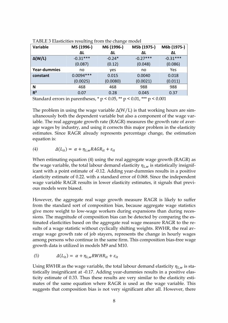
8

TABLE 3 Elasticities resulting from the change model

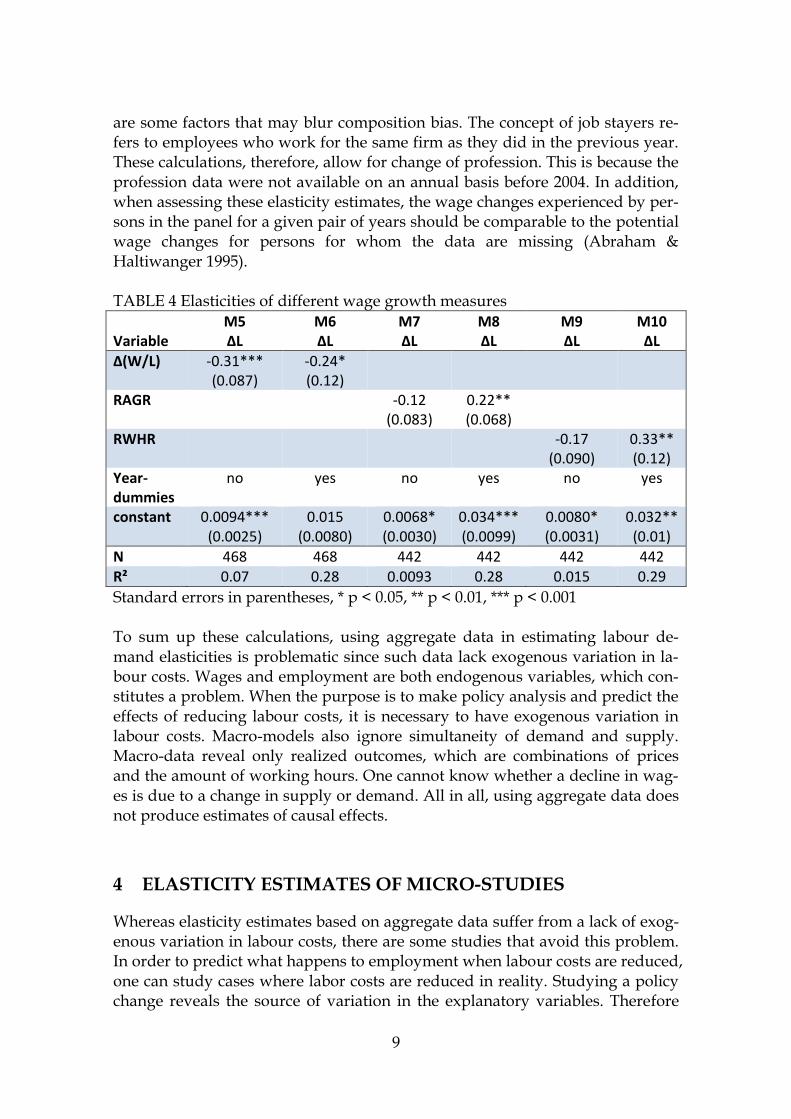
Standard errors in parentheses, * p < 0.05, ** p < 0.01, *** p < 0.001 The problem in using the wage variable Δ(W/L) is that working hours are sim-ultaneously both the dependent variable but also a component of the wage var-iable. The real aggregate growth rate (RAGR) measures the growth rate of aver-age wages by industry, and using it corrects this major problem in the elasticity estimates. Since RAGR already represents percentage change, the estimation equation is:

(4) 𝛥(𝐿𝑖𝑡) = 𝛼 + 𝜂𝐿,𝑤𝑅𝐴𝐺𝑅𝑖𝑡 + 𝜀𝑖𝑡

When estimating equation (4) using the real aggregate wage growth (RAGR) as the wage variable, the total labour demand elasticity 𝜂𝐿,𝑤 is statistically insignif-icant with a point estimate of -0.12. Adding year-dummies results in a positive elasticity estimate of 0.22. with a standard error of 0.068. Since the independent wage variable RAGR results in lower elasticity estimates, it signals that previ-ous models were biased. However, the aggregate real wage growth measure RAGR is likely to suffer from the standard sort of composition bias, because aggregate wage statistics give more weight to low-wage workers during expansions than during reces-sions. The magnitude of composition bias can be detected by comparing the es-timated elasticities based on the aggregate real wage measure RAGR to the re-sults of a wage statistic without cyclically shifting weights. RWHR, the real av-erage wage growth rate of job stayers, represents the change in hourly wages among persons who continue in the same firm. This composition bias-free wage growth data is utilized in models M9 and M10.

(5) 𝛥(𝐿𝑖𝑡) = 𝛼 + 𝜂𝐿,𝑤𝑅𝑊𝐻𝑅𝑖𝑡 + 𝜀𝑖𝑡

Using RWHR as the wage variable, the total labour demand elasticity 𝜂𝐿,𝑤 is sta-tistically insignificant at -0.17. Adding year-dummies results in a positive elas-ticity estimate of 0.33. Thus these results are very similar to the elasticity esti-mates of the same equation where RAGR is used as the wage variable. This suggests that composition bias is not very significant after all. However, there

Variable

M5 (1996-) ΔL

M6 (1996-) ΔL

M5b (1975-) ΔL

M6b (1975-) ΔL

Δ(W/L)

-0.31*** (0.087)

-0.24* (0.12)

-0.27*** (0.048)

-0.31*** (0.086)

Year-dummies no yes no Yes

constant

0.0094*** (0.0025)

0.015 (0.0080)

0.0040 (0.0021)

0.018 (0.011)

N 468 468 988 988

R² 0.07 0.28 0.045 0.37

9

are some factors that may blur composition bias. The concept of job stayers re-fers to employees who work for the same firm as they did in the previous year. These calculations, therefore, allow for change of profession. This is because the profession data were not available on an annual basis before 2004. In addition, when assessing these elasticity estimates, the wage changes experienced by per-sons in the panel for a given pair of years should be comparable to the potential wage changes for persons for whom the data are missing (Abraham & Haltiwanger 1995). TABLE 4 Elasticities of different wage growth measures

Variable

M5 ΔL

M6 ΔL

M7 ΔL

M8 ΔL

M9 ΔL

M10 ΔL

Δ(W/L)

-0.31*** (0.087)

-0.24* (0.12)

RAGR

-0.12 (0.083)

0.22** (0.068)

RWHR -0.17 (0.090)

0.33** (0.12)

Year-dummies

no yes no yes no yes

constant

0.0094*** (0.0025)

0.015 (0.0080)

0.0068* (0.0030)

0.034*** (0.0099)

0.0080* (0.0031)

0.032** (0.01)

N 468 468 442 442 442 442 R² 0.07 0.28 0.0093 0.28 0.015 0.29

Standard errors in parentheses, * p < 0.05, ** p < 0.01, *** p < 0.001 To sum up these calculations, using aggregate data in estimating labour de-mand elasticities is problematic since such data lack exogenous variation in la-bour costs. Wages and employment are both endogenous variables, which con-stitutes a problem. When the purpose is to make policy analysis and predict the effects of reducing labour costs, it is necessary to have exogenous variation in labour costs. Macro-models also ignore simultaneity of demand and supply. Macro-data reveal only realized outcomes, which are combinations of prices and the amount of working hours. One cannot know whether a decline in wag-es is due to a change in supply or demand. All in all, using aggregate data does not produce estimates of causal effects.

4 ELASTICITY ESTIMATES OF MICRO-STUDIES

Whereas elasticity estimates based on aggregate data suffer from a lack of exog-enous variation in labour costs, there are some studies that avoid this problem. In order to predict what happens to employment when labour costs are reduced, one can study cases where labor costs are reduced in reality. Studying a policy change reveals the source of variation in the explanatory variables. Therefore

10

using policy-induced variation in labour costs as quasi-experiments means that there is exogenous variation in labour costs. Such studies include exogenous variation in the price of labour, and therefore provide more reliable elasticity estimates. The resulting elasticities can be interpreted to be causal effects of re-ducing labour costs on employment. The difference-in-differences (DiD) method exploits policy changes as natural experiments. This strategy presupposes that one can define two groups, a treatment group and a control group, which share the same trend. When using the DiD method, one assumes that employment trends would be the same in both groups without the treatment, and that any deviation from this common trend is caused by the policy change (Angrist & Pischke 2009). When using this quasi-experimental method, one compares the growth in employment in the treated group to that of a control group. This kind of analysis offers more relia-ble results about how a reduction in labour costs affects employment (Johansen & Klette 1997). The relevant studies, their study designs and results are reported in table 5. Such studies provide the best available evidence of the effect on employment of reducing labour costs. The average labour demand elasticity of these studies is only -0.22. This is a significantly lower estimate than the result of the extensive meta-analysis of Lichter et al. (2014), which consisted of studies without exoge-nous variation. Studies containing exogenous variation in wages provide pref-erable estimates for policy analysis. Wage subsidies are an active labour market programme that create exogenous variation in labour costs. Kangasharju (2007) evaluates the effects of wage sub-sidies at the firm level in Finland during 1995- 2002. The analysis is based on the difference-in-differences method. The main finding is that wage subsidies seem to have stimulated employment in subsidized firms. According to the results, the estimated labour demand elasticity is -0.09 (with a t-value of 11.6). Payroll taxes in Finland include employer contributions to the employees’ pen-sion scheme, national pension insurance, unemployment insurance, national health insurance and employment accident insurance. Payroll tax cuts induce exogenous variation in labour costs, so they provide promising opportunities to estimate labour demand elasticities, which can be used to make causality inter-pretations. Egebark and Kaunitz (2013) use difference-in-differences (DiD) to investigate whether payroll tax cuts increase youth employment. The policy change exam-ined was enacted in 2007, when the Swedish employer-paid payroll tax rate was lowered by 11 percentage points for employees who at the start of the year had turned 18 but not 25 years of age. Their treatment group therefore consisted of people aged 19-25, while the control group consisted mainly of 26-year-olds. The estimated elasticity is -0.31.

11

TABLE 5 Elasticity estimates of micro-studies

Study Information Elasticity (s.e.)

Skedinger (2014)

Sweden, 2000-2011. 13,000 firms with a total of 300,000 employees. Large payroll tax cuts for young workers, two reforms in 2007 and 2009. DiD. Treat-ment group: workers aged 21-25. Control group 27-29-year-olds.

-0.19

(0.085)

Huttunen et al (2013)

Finland, a targeted low-wage subsidy experiment in 2006-2010. DiD. Eligible for the subsidy: workers over 54 years old, earning between €900 and €2,000 per month and working full-time. Control group: similar groups which were not eligible for the subsidy.

-0.13

(0.107)

Egebark & Kaunitz (2013)

Sweden, 2001-2010. Large payroll tax cut for young workers in 2007. DiD. Treatment group: workers aged 19-25. Control group: 26-year-olds.

-0.31

Korkeamäki & Uusitalo (2009)

Finland, 2003-2009. A regional experiment that re-duced payroll taxes by 3–6 percentage points for 3 years. Treatment group: firms in the 20 target munici-palities in northern Finland. Control group: similar firms in a comparison region of Eastern Finland.

-0.6

Bennmarker et al (2009)

Sweden, 2001-2004. 10 percentage point reduction in payroll tax in 2002 in northern Sweden. DiD. Annual firm-level data. Control group: similar firms operating in nearby regions.

+0.01 (0.1)

Bennmarker et al (2009)

Extending the analysis to include entry and exit of firms.

-0.38 (0.27)

Kangasharju (2007)

Finland, 1995-2002. Wage subsidy of 430-770€/month. Unbalanced panel of 31,000 firms. DiD. Subsidized firms vs. non-subsidized.

-0.09 (0.0078)

Kramarz & Philippon (2001)

France, 1990-1998. Tax subsidies. Workers directly affected by the changes vs. control group. Transition probabilities from non-employment to employment.

-0.03

Average elasticity

-0.215

Elasticity estimates obtained this way are useful for policy analysis because they are based on data that contain exogenous variation in labour costs. Unfor-tunately, the number of relevant micro-studies appears to be very limited. An-other problem is that the experiments investigated were only temporary. In ad-dition, there are grounds to doubt whether the results of these experiments can be generalized to the overall economy. However, many of these experiments are aimed at groups in which the elasticities should, in fact, be higher than on average.

12

There are many similar studies that are unable to estimate labour demand elas-ticities. Findings from many studies in Finland, Sweden and Norway show that a payroll tax cut is likely to push wages up. Johansen and Klette (1997) examine the effects of regional differences in payroll taxes in Norway, and find that changes in payroll taxes are for the most part shifted to wages. Bohm and Lind (1993) evaluate the employment effects of regional wage subsidies in Northern Sweden. Bennmarker, Mellander and Öckert (2009) and Korkeamäki and Uu-sitalo (2009) evaluate the effects of regional wage subsidies in Sweden and Fin-land. They all share the same finding that changes in payroll taxes are partly shifted to wages with little effect on employment. Such studies do not provide elasticity estimates since labour costs remained unchanged.

5 CONCLUSIONS

The calculations in this report show that estimating labour demand elasticities based on aggregate data has a tendency to produce biased and excessively large elasticity estimates. Using aggregate data in estimating labour demand elastici-ties is problematic since such data lack exogenous variation in labour costs. This makes it impossible to measure the causal impacts of labour costs on employ-ment. When the purpose is to conduct policy analysis and predict the effects of reducing labour costs, there should be exogenous variation in labour costs. In order to predict what happens to employment when labor costs are reduced one can study cases where labor costs are reduced in reality. Using policy-induced variation in labour costs as quasi-experiments means that there is ex-ogenous variation in the price of labour. This provides more reliable elasticity estimates that can be interpreted as causal effects of reducing labour costs on employment. This report contains a brief meta-analysis of micro-studies that examine situations where labour costs have been changed exogenously. Unfor-tunately, the number of relevant micro-studies appears to be very limited. However, such studies provide the best available evidence of the effect on em-ployment of reducing labour costs. The average labour demand elasticity of these studies is -0.22. The estimated employment effects of the competitiveness pact are sensitive to the elasticity estimate used in it. The elasticity estimate used appears to be very high, predicting overly optimistic employment effects. The Ministry of Fi-nance’s estimate of 35,000 new jobs is based on an elasticity estimate of -0.7. However, as this report shows, this high elasticity appears to be upwards-biased. Unfortunately, this in turn suggests that the real employment effects are likely to be below expectations.

13

REFERENCES

Abraham, K., Haltiwanger, J. C. (1995). Real Wages and the Business Cycle.

Journal of Economic Literature 33, 1215–64. Andersen, T., Kotakorpi, K., Laakso, L., Puhakka, M. & Uusitalo, R. (2016).

Finnish Economic Policy Council Report 2015. Angrist, J. D. – Pischke J. (2009): Mostly Harmless Econometrics – An Empiri-

cist’s Companion, Princeton University Press. Bennmarker, H., E. Mellander, and B. Öckert (2009). Do regional payroll tax re-

ductions boost employment? Labour Economics 16 (5), 480 - 489. Bohm, P. and H. Lind (1993). Policy evaluation quality : A quasi-experimental

study of regional employment subsidies in sweden. Regional Science and Urban Economics 23 (1), 51-65.

Bowlus, A., Liu, H., Robinson, C. (2002). Business Cycle Models, Aggregation, and Real Wage Cyclicality. Journal of Labor Economics, 2002, vol. 20, no. 2, pt. 1

Egebark, J. and Kaunitz, N. (2013). Do payroll tax cuts raise youth employment? Manuscript, Department of Economics, Stockholm University.

Gruber, J. (1994). The incidence of mandated maternity benefits. American Eco-nomic Review, 84 (3), 622–641.

Gruber, J. (1997). The incidence of payroll taxation: evidence from Chile. Journal of Labor Economics, 15 (3, Part 2).

Hamermesh, D. (1993). Labor Demand, Princeton University Press, Princeton. Hamermesh, D. (1986). The Demand for Labor in the Long Run. Handbook of

Labor Economics, Volume 1. Edited by O. Ashenfelter and R. Layard, Elsevier Science Publishers BV.

Honkapohja, S., Koskela, E., ja Uusitalo, R. (1999). Työllisyys, työn verotus ja julkisen talouden tasapaino. Kansantaloudellinen aikakauskirja 1/2009.

Huttunen, K., J. Pirttilä, and R. Uusitalo (2013). The employment effects of low-wage subsidies. Journal of Public Economics 97 (0), 49 - 60.

Johansen, F. and Klette, T. (1997). Wage and Employment Effectsof Payroll Tax-es and Investment Subsidies. Statistics Norway Research Department.

Kangasharju, A. (2007). Do Wage Subsidies Increase Employment in Subsidized Firms? Economica, New Series, Vol. 74, No. 293 (Feb., 2007), pp. 51-67

Kauhanen, A., Maliranta, M. (2012). The Roles of Job and Worker Restructuring in Aggregate Wage Growth Dynamics. The Research Institute of the Finn-ish Economy ETLA.

Korkeamäki, O. and R. Uusitalo (2009). Employment and wage effects of a pay-roll-tax cut - evidence from a regional experiment. International Tax and Public Finance 16, 753 - 772.

Korkeamäki, O. (2011). The Finnish payroll tax cut experiment revisited, Work-ing Paper 22, Government Institute for Economic Research, Helsinki.

Kramarz, F. and Philippon, T. (2001), The impact of differential payroll tax sub-sidies on minimum wage employment, Journal of Public Economics 82, 115-146.

14

Lichter, A., Peichl, A. ja Siegloch, S. (2014), The Own-Wage Elasticity of De-mand of Labor Demand: A Meta-Regression Analysis. IZA DP No. 7958.

Official Statistics of Finland (OSF): Financial statements inquiry for enterprises. [e-publication]. Helsinki: Statistics Finland. [referred: 14.10.2016]. Access method: <http://tilastokeskus.fi/keruu/yrti/index.html>

Official Statistics of Finland (OSF): Labour force survey [e-publication]. ISSN=1798-7857. Helsinki: Statistics Finland. [referred: 13.7.2016]. Access method: <http://www.stat.fi/til/tyti/yht_en.html>

Official Statistics of Finland (OSF): Productivity surveys [e-publication]. ISSN=2343-4333. Helsinki: Statistics Finland [referred: 13.7.2016]. Access method: <http://www.stat.fi/til/ttut/meta_en.html>

Official Statistics of Finland (OSF): Time use survey. [e-publication]. Helsinki: Statistics Finland. [referred: 14.10.2016]. Access method: <http://tilastokeskus.fi/keruu/aja/index_en.html>

Skedinger, P. (2014). Effects of Payroll Tax Cuts for Young Workers. Nordic Economic Policy Review 2014(1), 126 - 169.

Solon, G., Barsky, R., Parker, J. A. (1994). Measuring the Cyclicality of Real Wages: How Important Is Composition Bias? Quarterly Journal of Eco-nomics 109: 1–26.

Stokke, H. (2015). Regional payroll tax cuts and individual wages: Heterogene-ous effects across education groups. Department of Economics, Norwe-gian University of Science and Technology.

Valtiovarainministeriön muistio. (1.3.2016). Pika-arvio kilpailukykysopimuksen vaikutuksista.

Valtiovarainministeriön muistio. (29.9.2015). Hallitusohjelman mukaisen palk-kamaltin ja yksikkötyökustannusten alentamisen vaikutuksista.

15

APPENDIX

Industries in calculations Standard Industrial Classification TOL 2008

Average of annual total working hours

by industry (1975-2014) (1 000 000 h)

05-09 Mining and quarrying 9.2

10-12 Manufacture of food products, beverages, and tobacco products

64.0

13-15 Manufacture of textiles, wearing apparel, and leather and related products

22.5

16 Manufacture of wood and of products of wood and cork 44.5

17 Manufacture of paper and paper products 50.6

18 Printing and reproduction of recorded media 21.3

23 Manufacture of other non-metallic mineral products 25.7

24 Manufacture of basic metals 26.1

25 Manufacture of fabricated metal products, except machin-ery and equipment

68.5

26-27 Manufacture of computer, electronic and optical products; Manufacture of electrical equipment

92.6

28 Manufacture of machinery and equipment n.e.c. 76.3

29-30 Manufacture of motor vehicles, trailers and semi-trailers Manufacture of other transport equipment

28.9

31-32 Manufacture of furniture Other manufacturing

28.9

33 Repair and installation of machinery and equipment 32.2

35-39 Electricity, gas, steam and air conditioning supply Water supply; sewerage, waste management and remedia-tion activities

38.9

41-43 Construction 240.6

45-47 Wholesale and retail trade; repair of motor vehicles and motorcycles

459.6

49-53 Transportation and storage 221.3

55-56 Accommodation and food service activities 119.6

58-63 Information and communication 143.6

64-66 Financial and insurance activities 70.8

68 Real estate activities 35.1

69-75 Professional, scientific and technical activities 143.1

77-82 Administrative and support service activities 124.9

84-88 Public administration and defence; compulsory social se-curity; Education; Human health and social work activities

73.8

90-93 Arts, entertainment and recreation 20.4