Demand forecasting is the activity of estimating the quantity of a product or service that consumers will purchase. Demand forecasting involves techniques including both informal methods, such as educated guesses, and quantitative methods, such as the use of historical sales data or current data from test markets. Demand forecasting may be used in making pricing decisions, in assessing future capacity requirements, or in making decisions on whether to enter a new market.

I. It is the most important function of managing .

II. To minimize the risks arising out of an uncertain future.

III.The risks associated with uncertain future can be negated if one tries to make reasonable assumptions about the course that the future is likely to take.

IV.Helpful in better planning and allocation of natural resources.

V. To determine industry demand.

VI.Needed as market conditions are not stable.

VII.Helps in assessing demand of a commodity in the market.

Types of demand

forecasting

Short-termforecast

Long-termforecast

I. Short-term forecast –

The short-term forecast helps in preparing suitable sales policies and proper scheduling of output to avoid over stocking etc. It also helps in arriving at suitable promotional activities such as advertising and sales promotions.

II. Long-term forecast –

Long-term forecast helps in capital planning. The mngrs on the top invest huge amount in everything needed to meet the demand estimated through long-term forecast. It helps in saving wastages in time , material etc..

I. Short-term forecasting- usually 1year , long-term forecasting- 5-20 years

II. Levels of forecasting –

(a). Macro level

(b). Industry-level

(c). Firm-level

III.Forecasts should be general/specific

IV.Methods of forecasting –

The methods of forecasting are usually different for new products and the old ones.

V. The product and marketic conditions must be taken into

account.

VI.Demand forecasting is important to classify products as product goods , consumer durable or goods and services. Economic analysis indicates distinctive patterns of demand for each of these different categories.

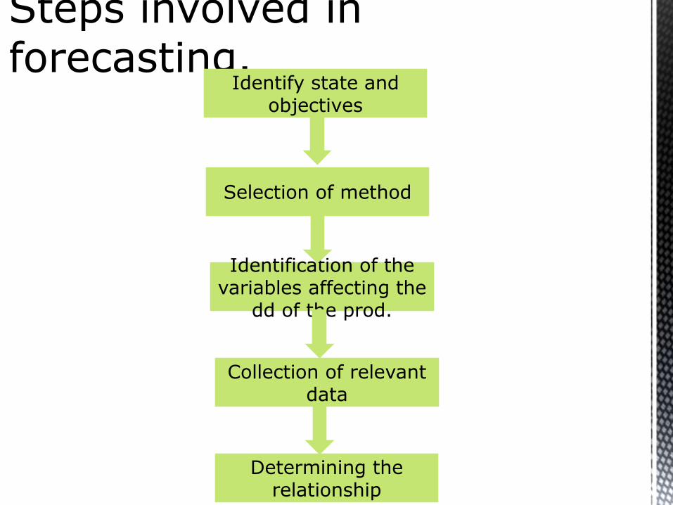
Identify state and objectives

Selection of method

Identification of the variables affecting the

dd of the prod.

Collection of relevant data

Determining the relationship

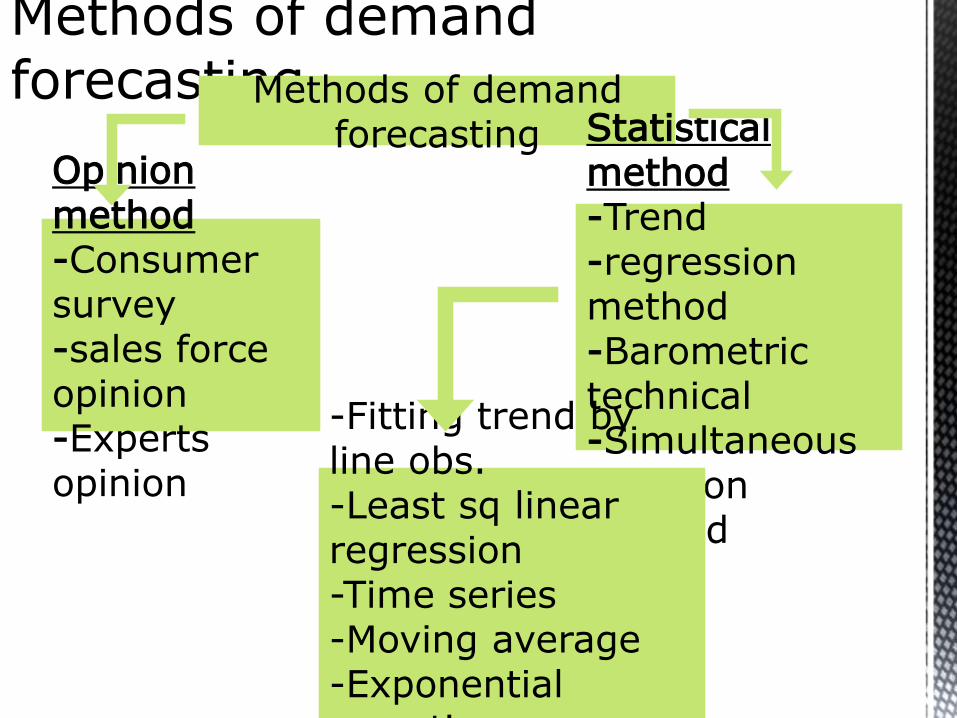
Methods of demand forecasting

Opinion method-Consumer survey-sales force opinion-Experts opinion

Statistical method-Trend -regression method-Barometric technical -Simultaneous equation method

-Fitting trend by line obs.-Least sq linear regression-Time series-Moving average-Exponential smooting

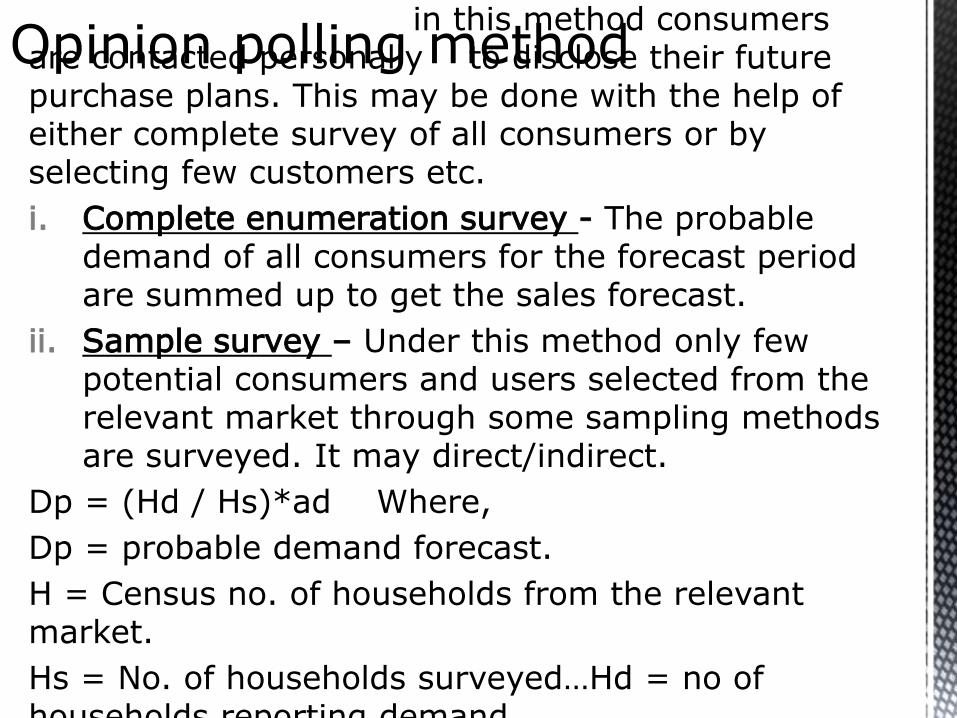
(a). Consumer’s survey –

in this method consumers are contacted personally to disclose their future purchase plans. This may be done with the help of either complete survey of all consumers or by selecting few customers etc.

i. Complete enumeration survey - The probable demand of all consumers for the forecast period are summed up to get the sales forecast.

ii. Sample survey – Under this method only few potential consumers and users selected from the relevant market through some sampling methods are surveyed. It may direct/indirect.

Dp = (Hd / Hs)*ad Where,

Dp = probable demand forecast.

H = Census no. of households from the relevant market.

Hs = No. of households surveyed…Hd = no of households reporting demand

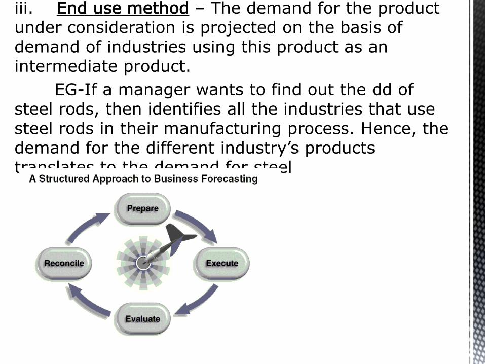
iii. End use method – The demand for the product under consideration is projected on the basis of demand of industries using this product as an intermediate product.

EG-If a manager wants to find out the dd of steel rods, then identifies all the industries that use steel rods in their manufacturing process. Hence, the demand for the different industry’s products translates to the demand for steel

(b). Sales force opinion(collective opinion) –

Sales men are required to estimate expected sales in their allotted region or territory. The whole estimates and aggregated responses from the consumer are summed up to forecast.

DISADVANTAGES1)It is almost completely subjectively as personnel opinion can possibly influence the forecast.2)The usefulness of this method is restricted to short term changes.3)The salesmen may be unaware of the broader economic changes likely to have an impact on the future demand.

ADVANTAGES1).This method is simplified and does not involve the use of statistical techniques.2)The forecasts are based on the first hand knowledge of salesman.

The experts in the field are asked to provide their own estimates of likely sales. Experts may include managers , dealer’s suppliers , consultants , officers of trade associations etc., this method is best suited in situations where changes are occurring.

For example , forecasting future technology status. The experts may give divergent view but it is helpful to the managers to adopt new ideas on the basis of these views.

(d). Delphi technique –

Delphi method is a variant of the opinion pool and expert opinion. This method consists of attempt to arrive at consensus in a uncertain area by questioning a group of experts. This method is highly effective because of the nature of the experts pooled in together. The technique comes with an conclusion about the future forecast

The statistical methods are frequently used to project demand.

i. Trend projection method ii. Regressions method iii. Barometric method

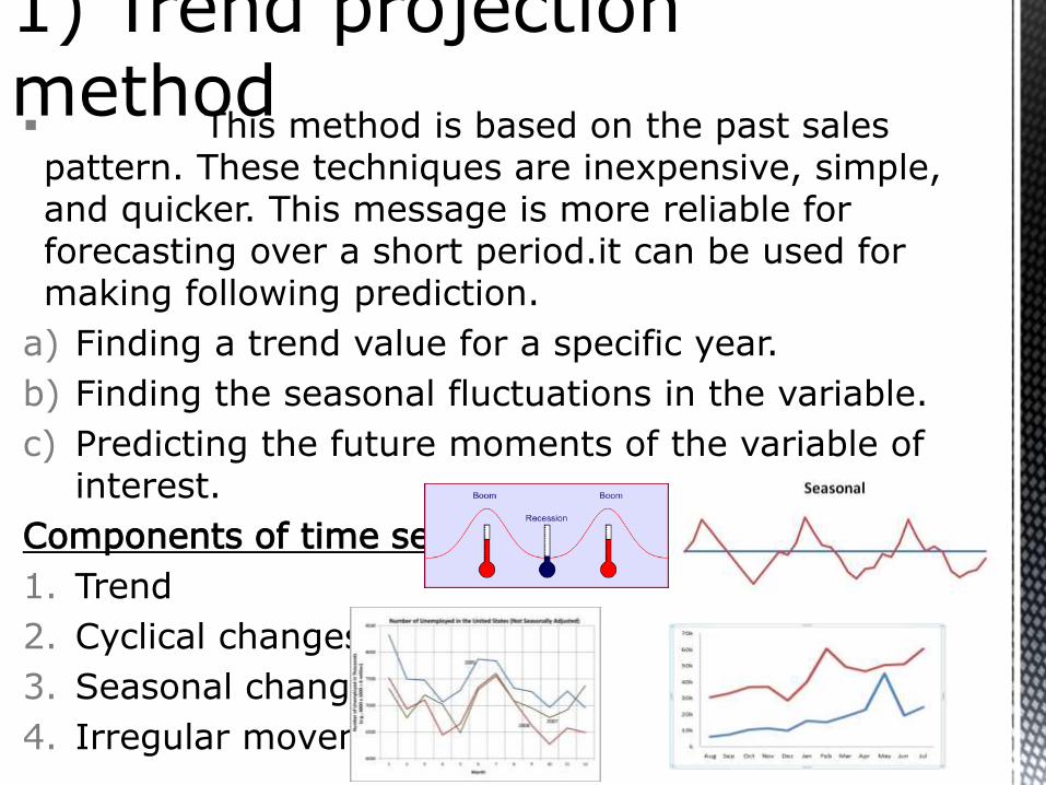
This method is based on the past sales pattern. These techniques are inexpensive, simple, and quicker. This message is more reliable for forecasting over a short period.it can be used for making following prediction.

a) Finding a trend value for a specific year.

b) Finding the seasonal fluctuations in the variable.

c) Predicting the future moments of the variable of interest.

Components of time series –

1. Trend

2. Cyclical changes

3. Seasonal changes

4. Irregular movement

1. Trend – The trend component of a time series in the overall direction of the movement of the variable over a long period.

2. Cyclical changes – The cycle component of a time series is a wave like, retentive movement fluctuating about the trend of the series(EXAMPLE: depression, recovery, prosperity and recession).

3. Seasonal changes – The seasonal movements of time series are that repetitive, fluctuating movement that always occurs at a particular time of the year. E.g. - sale of umbrella go up during rain seasons and demand for woollen cloths go up during the winter season.

4. Irregular movement – These are those variations that are left over after isolating the other components. E.g. – a sudden outbreak of epidemics may increase the sales of drugs.

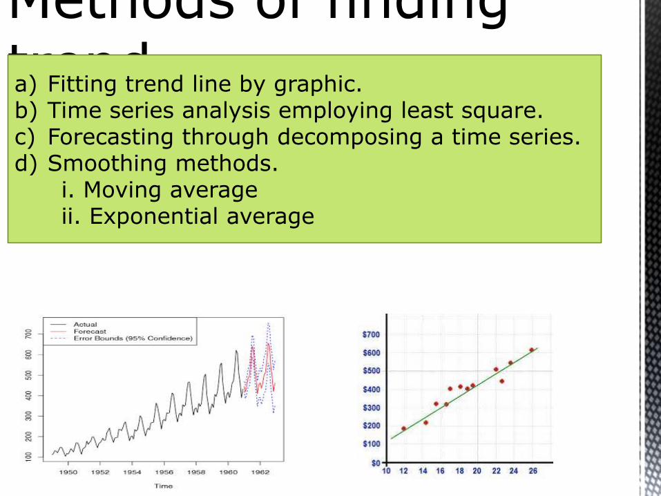
a) Fitting trend line by graphic.b) Time series analysis employing least square.c) Forecasting through decomposing a time series.d) Smoothing methods.

i. Moving averageii. Exponential average

plotting of annual sales on graph, and then estimating demand by observing where the trend line lies.

B. Time series analysis employing least squares methods – this technique is most widely used in practise. It is a statistical method, with its help a trend line is fitted to the data. This line is known as “The line of best fit”. By extrapolating the trend line for future we can get the corresponding figures of forecasting sales. In this analysis there is only one independent variable time. This system of forecasting is considered negative because it does not explain the reason for the changes.

C. Forecasting through decomposing a time series –Time series is composed of trend seasonal fluctuations, cyclical movements and irregular variations. If the available data is quarter wise/month wise, it is possible to identify the seasonal effect. If this data is available for sufficiently long period of time the trends and

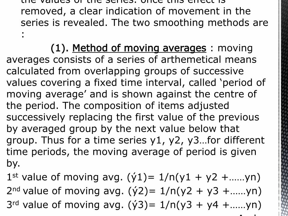
the values of the series. once this effect is removed, a clear indication of movement in the series is revealed. The two smoothing methods are :

(1). Method of moving averages : moving averages consists of a series of arthemetical means calculated from overlapping groups of successive values covering a fixed time interval, called ‘period of moving average’ and is shown against the centre of the period. The composition of items adjusted successively replacing the first value of the previous by averaged group by the next value below that group. Thus for a time series y1, y2, y3…for different time periods, the moving average of period is given by.

1st value of moving avg. (ý1)= 1/n(y1 + y2 +……yn)

2nd value of moving avg. (ý2)= 1/n(y2 + y3 +……yn)

3rd value of moving avg. (ý3)= 1/n(y3 + y4 +……yn)

And so

when the period of moving average is odd (i.e.) if ‘ n ’ is odd the successive value of moving averages is against the middle value of the concerned group of item. For example if n = 9, the first moving avg. value is placed against the middle period i.e. 5th

value, the second moving avg. value is placed against the time period 6 and so on.

when the period of moving average ‘ n ’ is even, then there are two middle periods. In order to synchronize the moving avg. with original data, we take a two-period average of the moving average and place them in between the corresponding time periods.

very popular approach for short-term forecasting. This method determines the values by computing exponentially weighted system. The weight assigned to each reflects the degree of importance of that value. More recent values being more relevant for the forecast are assigned greater than weights than previous period’s values.it may be noted that weights (w) are to be assigned that ‘w’ lies between zero and unity (0 < w < 1).

To describe the process of exponential smoothing, let y1, be the observed value of the series at time ‘ t ’ and ‘St’ be the smoothing value at the time ‘ t ’. The smoothing scheme begins setting smoothing values equal to observed value for the period (t=1); St = y1 and for any succeeding time period t, the smoothen value St is found with the help of the equation :

St = wy1 + (1 - w )St - 1

That is current smoothen value = w current value observed value + [(1 - w)

ARIMA(auto-regression integrated moving averages) –this method of forecasting was developed by Box and Jenkins. This method is highly suitable situations where the pattern in the underlying series is highly compels and is difficult to understand. This method combines smoothing with auto-regressive method. It is primarily for short term forecasting.

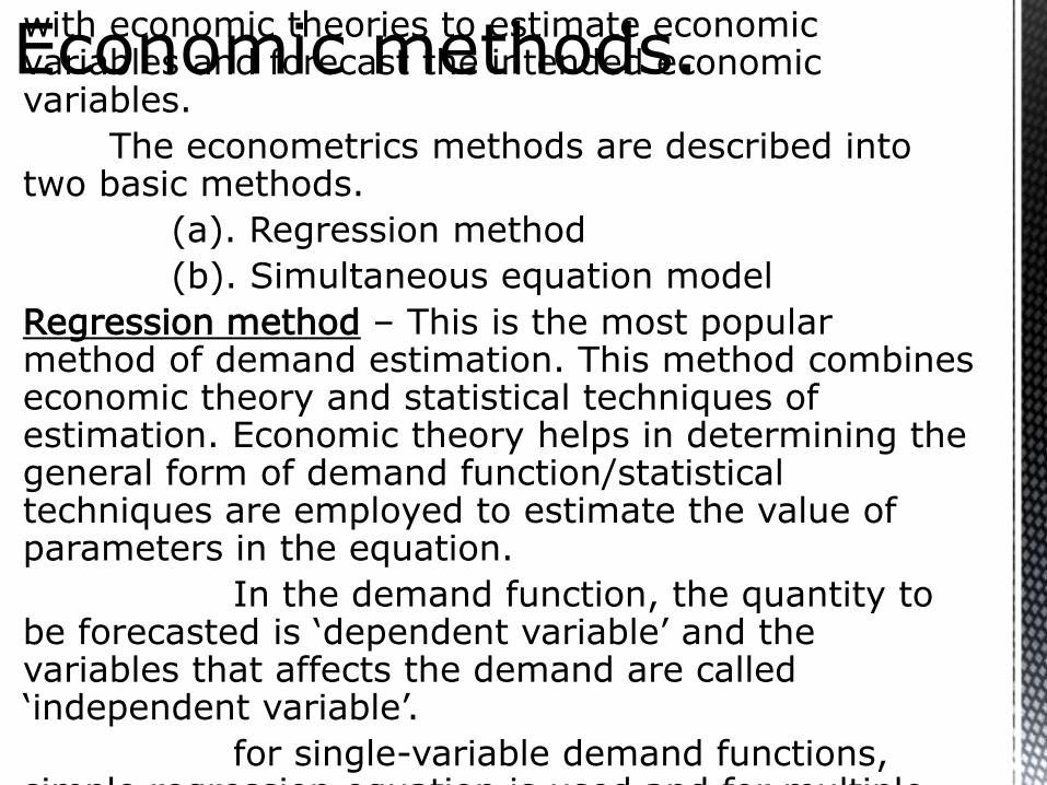
Econometric methods combine statistical tools with economic theories to estimate economic variables and forecast the intended economic variables.

The econometrics methods are described into two basic methods.

(a). Regression method

(b). Simultaneous equation model

Regression method – This is the most popular method of demand estimation. This method combines economic theory and statistical techniques of estimation. Economic theory helps in determining the general form of demand function/statistical techniques are employed to estimate the value of parameters in the equation.

In the demand function, the quantity to be forecasted is ‘dependent variable’ and the variables that affects the demand are called ‘independent variable’.

for single-variable demand functions, simple regression equation is used and for multiple

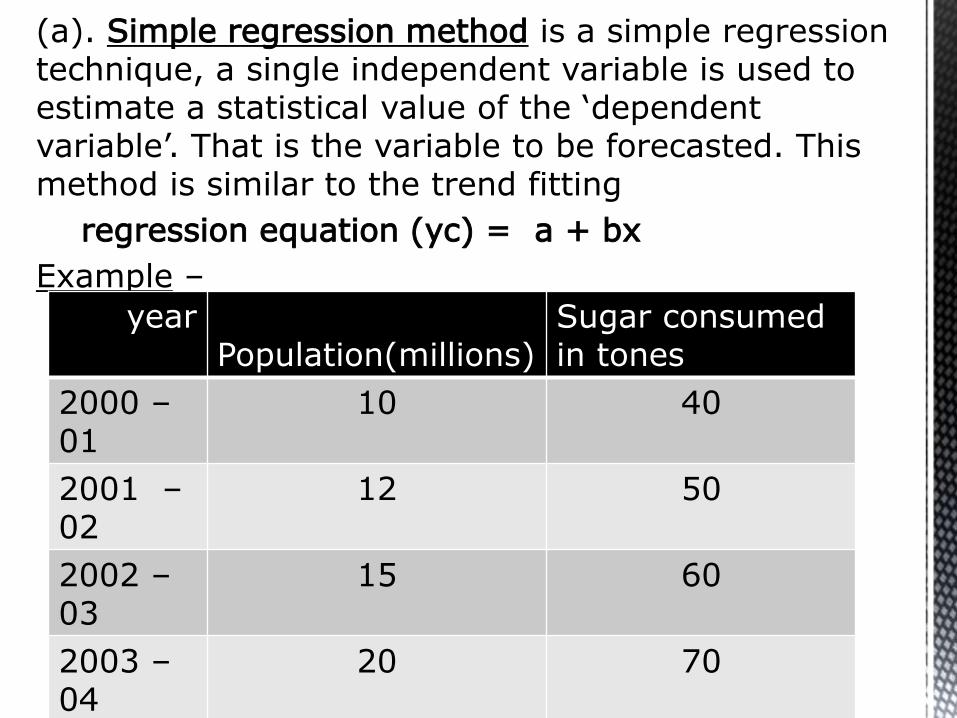
(a). Simple regression method is a simple regression technique, a single independent variable is used to estimate a statistical value of the ‘dependent variable’. That is the variable to be forecasted. This method is similar to the trend fitting

regression equation (yc) = a + bx

Example –

yearPopulation(millions)

Sugar consumed in tones

2000 –01

10 40

2001 –02

12 50

2002 –03

15 60

2003 –04

20 70

2004 – 25 80

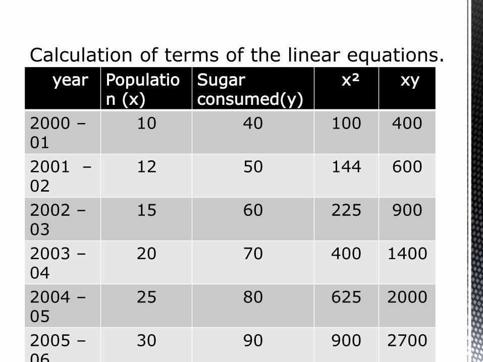
year Population (x)

Sugarconsumed(y)

x² xy

2000 –01

10 40 100 400

2001 –02

12 50 144 600

2002 –03

15 60 225 900

2003 –04

20 70 400 1400

2004 –05

25 80 625 2000

2005 –06

30 90 900 2700

Linear equations :

Ty = na + b(Tx)

Txy = Tx(a) + bx²

By substituting the values in the above equations we get,

490 = 7a + 152b (1)

1200 = 1562a + 3994b (2)

By solving equation (1) & (2) we get,

a = 27.44.

b = 1.96 and

By substituting values for a and b, we get the estimated regression equation as –

Yc = 27.44 + 1.96x

Suppose the population for 2008-09 is projected to be 70million the demand for sugar in 2008-09 maybe estimated as-

Yc = 27.44 + 1.96(70) = 137millon tones.

(b). Multi-variant regression is used where demand for a commodity is deemed to be the function of a co-variables or in cases where the number of explanatory variable is greater than one.

Simultaneous equation model –

The simultaneous equation of forecasting involves estimating several simultaneous questions. These equations are, generally, behavioural equations, mathematical identities and market clearing equations.

The simultaneous equations method is a complete and systematic approach to forecast.

The first step in this technique is to develop a complete model and specify the behavioural assumptions regarding variables included in the model. The variables that are included in the model are called –

(i). Endogenous variables and

(ii). Exogenous variables

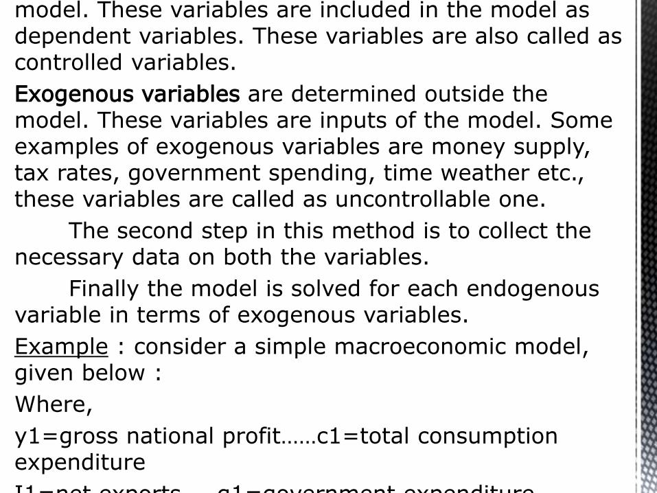
Endogenous variables are determined within the model. These variables are included in the model as dependent variables. These variables are also called as controlled variables.

Exogenous variables are determined outside the model. These variables are inputs of the model. Some examples of exogenous variables are money supply, tax rates, government spending, time weather etc., these variables are called as uncontrollable one.

The second step in this method is to collect the necessary data on both the variables.

Finally the model is solved for each endogenous variable in terms of exogenous variables.

Example : consider a simple macroeconomic model, given below :

Where,

y1=gross national profit……c1=total consumption expenditure

I1=net exports……g1=government expenditure

The barometric method of forecast follows the method meteorologist’s use in weather forecasting. Meteorologists use the barometer to forecast weather conditions on the basis of movements of mercury in the barometer. Following the logic of this method, many economists use economists use economic indicators as a barometer to forecasts to forecast trends in business activities. The method was first developed and used in the year 1920 by Harvard economic service.

The indicators used in this method are –

(i). Leading indicators

(ii). Coincidental indicators

(iii). Lagging indicators

ahead of some other series. Example : index of net business, new orders for durable goods, new building permit, corporate profit after tax.

ii. Coincidental indicators – which move up or down simultaneously with the level of economic activity. Examples : no. of employees in the non-agricultural sector, rate of unemployment gross national product, sales recorded by the manufacturing etc.

iii. Lagging indicators – consists of all those indicators which follow a change after sometime. Example – outstanding loans, lending rate for short-term loan, labour cost per unit of manufacturer output.