Monetary Theory and Policy

•Demand and supply of money•The supply of money and the equilibrium interest rate•The monetary transmission mechanism•The Quantity theory of money•The record of monetary policy

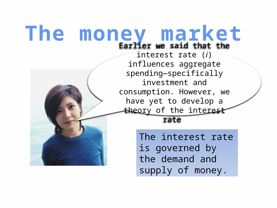
The money marketEarlier we said that the interest rate (i) influences aggregate spending—

specifically investment and consumption. However, we have yet to develop a theory of the interest

rate

The interest rate is governed by the demand and supply of money.

Why do agents hold money?

1. To make planned expenditures/payments

2. To be prepared for unexpected expenditures/payments.

3. To store wealth.

The interest rate ( i) measuresthe opportunity cost of

holding money

The higher the interest rate, the more interest I give up by

holding my wealth in money-- as opposed to an

interest-bearing asset.

5

Inte

rest

rate

0 Quantity of money

Dm

The money demand, Dm, slopes downward. As the interest rate falls, other things constant, so does the opportunity cost of holding money; the quantity of money demanded increases.

Demand for money

The supply of moneyWe assume that the Fed (or

central banks generally) determines the supply of

money

7

Effect of an increase in the money supply

Dm

Because the money supply is determined by the Federal Reserve, it can be represented by a vertical line.

0 Quantity of moneyM M’

SmS’m

b

a

Inte

rest

rate

i

i’

At point a, the intersection of the money supply, Sm, and the money demand, Dm, determines the market interest rate, i.Following an increase in the money supply to S’m, the quantity of money supplied exceeds the quantity demanded at the original interest rate, i.

People attempt to exchange money for bonds or other financial assets. In doing so, they push down the interest rate to i’, where quantity demanded equals quantity supplied. This new equilibrium occurs at point b.

8

Effects of an increase in the money supply on interest rates, investment, and aggregate demand

An increase in the money supply drives the interest rate down to i'.

Dm

0 MoneyM M’

Sm S’m

b

a

Inte

rest

rate

i

i’

(a) Supply and demand for money

DI

0Investment

I I’

Inte

rest

rate

i

i’

(b) Demand for investment

With the cost of borrowing lower, the amount invested increases from I to I‘.

This sets off the spending multiplier process, so the aggregate output demanded at price level P increases from Y to Y ‘

AD

0 Real GDPY Y’

Pric

e le

vel

P

(c) Aggregate demand

AD’b

ab

a

Chain of cause and eff ect

M↑→i↓→I↑→AD↑→Y↑

The transmission mechanism

Fed open market purchase injects reserves into the banking system

Commercial banks, thrifts, etc. expand loans and deposits

The money supply increases

The equilibrium interest rate decreases

Consumption and investment increase

Real GDP, employment, and (perhaps ) the price level increase

11

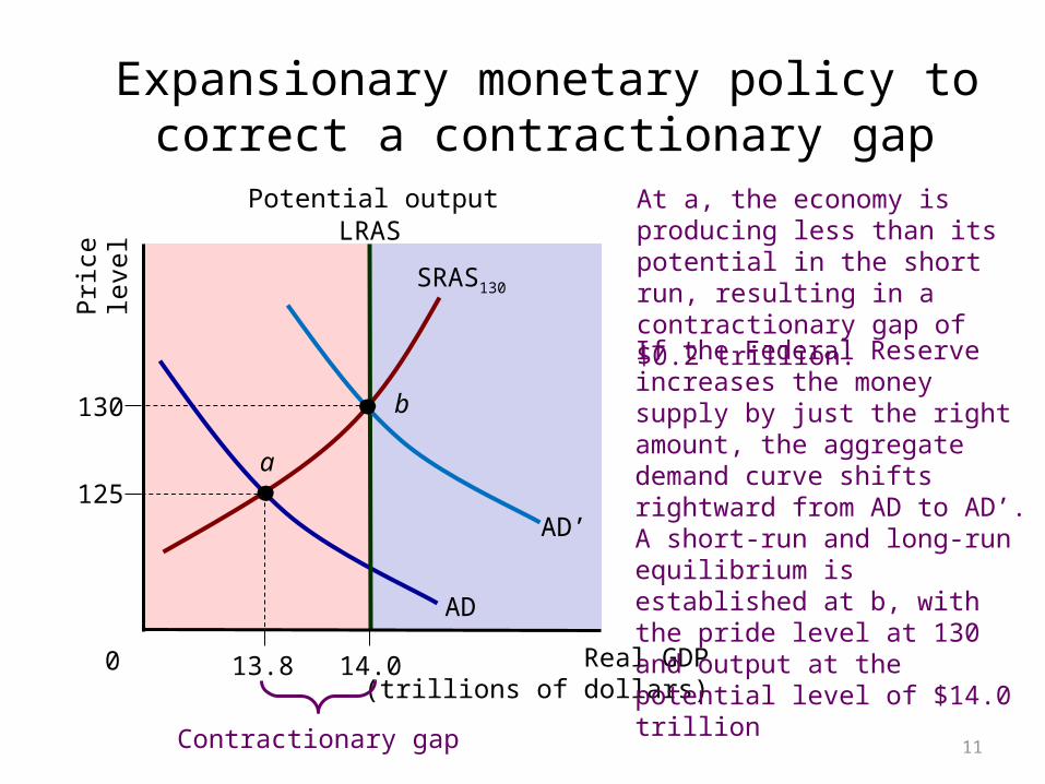
Expansionary monetary policy to correct a contractionary gap

Pric

e le

vel

125

130

AD

SRAS130

a

Potential outputLRAS

At a, the economy is producing less than its potential in the short run, resulting in a contractionary gap of $0.2 trillion.

Real GDP (trillions of dollars)

0 14.013.8

AD’

b

If the Federal Reserve increases the money supply by just the right amount, the aggregate demand curve shifts rightward from AD to AD’. A short-run and long-run equilibrium is established at b, with the pride level at 130 and output at the potential level of $14.0 trillion

Contractionary gap

The FOMC sets a target for the “federal funds” rate, which is the rate that banks

charge other banks for “borrowed” reserves.

13

Recent ups and downs in the federal funds rate

Since the early 1990s, the Fed has pursued monetary policy primarily through changes in the federal funds rate, the rate that banks charge one another for borrowing and lending excess reserves overnight.

Global financialcrisis promptsrate cuts

Rate cuts to combat recession

Rate increased to slow red-hot economy

Rate cuts to limit impact of mortgage defaults on economy

Rate increase to head off inflation

The Fed has cut rates sharply in 2008

The Equation of Exchange

YPVM Where

•M is the quantity of money

•V is the velocity of circulation

•P is the price level

•Y is real GDP

What is velocity (V)?

MYPV )(

Velocity (V) is the average number of times per year a unit of money is spent for new goods and services. Let

(P Y) is nominal GDP. Let P = 1.25; Y = $8 trillion; and M= $2 trillion. Thus:

trillion $2 trillion)8$25.1( V

Or, V = 5

Money and Aggregate Demand in LR

• Velocity depends on– Customs and convention of commerce

• Innovations facilitate exchange• Higher velocity

– Frequency • The more often workers get paid

– Higher velocity

– Stability (store of value)• The better store of value

– Lower velocity

17

Equation of Exchange is Always True

The equation simply states that what is spent for new goods

and services (M V) is equal to the market value of new goods and services produced (P Y).

Illustration

trillion$105 trillion2$ VM

trillion$10 trillion$825.1$ YP

Using the numbers on a preceding slide, we can see that

and

trillion$10 YPVM

thus

“Monetarist” interpretation of the equation of exchange

“Inflation is always and everywhere a monetary phenomenon.”

The monetarists believe that price level changes (hence inflation) can be explained by changes in

quantity of money

Example

Assume that V = 5 and is constant. Y is $8 trillion

(also assumed to be constant). Initially, let M =

$2 trillion

YVMP )(

1.25 trillion8$)5 trillion 2($ P

1.50 trillion8$)5 trillion 4.2($ P

percent 20 trillion $2100 trillion)$2 - trillion 4.2($

percent 20 1.251001.25) - 5.1(

Our basic equation can be rearranged as follows:

Now solve for the price level (P):

Now let the money supply increase to $2.4 trillion. Notice that:

Thus we have:

Notice that:

Hence a 20 percent increase in the money supply causes the price level to increase by 20

percent. Monetarists put the blame for inflation

squarely at the doorstep of the monetary authorities

(in the U.S., the FED).

24

In the long run, an increase in the money supply results in a higher price level, or inflation

Pric

e le

vel

130

140

AD

Potential outputLRAS

Real GDP (trillions of dollars)

0 14.0

AD’

b

The quantity theory of money predicts that if velocity is stable, then an increase in the supply of money in the long run results in a higher price level, or inflation. Because the long-run aggregate supply curve is fixed, increases in the money supply affect only the price level, not real output.a

25

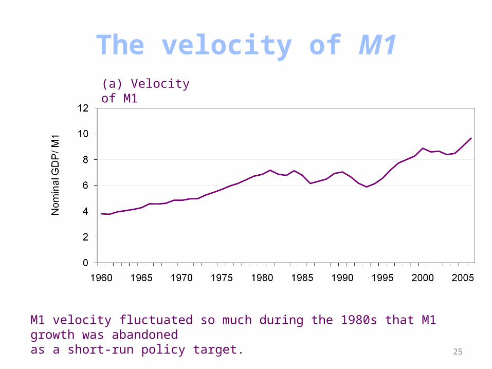
M1 velocity fluctuated so much during the 1980s that M1 growth was abandonedas a short-run policy target.

(a) Velocity of M1

The velocity of M1

26

M2 velocity appears more stable than M1 velocity, but both are now considered by the Fed as too unpredictable for short-run policy use.

(b) Velocity of M2

The velocity of M2

German Hyperinflation and Money

• A decade of annual inflation and money growth in 85 countries (average annual percent)

30

Record indicates that nations with high rates of monetary growth also suffer high rates of inflation

31

Targeting interest rate vs. targeting the money supply

An increase in the price level or in real GDP, with velocity stable, shifts rightward the money demand curve from Dm to D'm.

Dm

0 Quantity of moneyM M’

Sm S’m

e

Inte

rest

rate i’

i

D’m

e’’

e’If the Federal Reserve holds the money supply at Sm, the interest rate rises from i (at point e) to i ' (at point e').

Alternatively, the Fed could hold the interest rate constant by increasing the supply of money to S'm. The Fed may choose any point along the money demand curve D'm.

The Fed pulled on the string big time beginning in 1979—it was an anti-inflation strategy under Chairman

Paul Volcker

Potential GDP AS

AD1

Real GDP

Price Level

0

AD2

Modeling Contractionary Monetary Policy

Y1

8

10

12

14

16

18

20

79:01 79:07 80:01 80:07 81:01 81:07 82:01 82:07 83:01

Federal Funds

Recessions are shaded

6

8

10

12

14

16

18

20

80 82 84 86 88 90 92

Mortgage Interest Rates

Recessions are shaded

Conventional 30 year

www.economagic.com

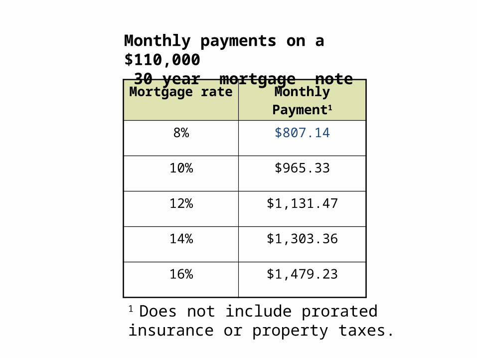
Mortgage rate

Monthly Payment1

8% $807.14

10% $965.33

12% $1,131.47

14% $1,303.36

16% $1,479.23

1 Does not include prorated insurance or property taxes.

Monthly payments on a $110,000 30 year mortgage note

400

800

1200

1600

2000

2400

80 82 84 86 88 90 92

Monthly Housing Starts

Recessions are shadedData in thousands of units

www.economagic.gov

More recently, the Fed raised the federal funds rate six times between May 1999

and May 2000—from 4.75% to 6.5 %.

Evidently unemployment was getting “too low.”

The FOMC reversed course in July 2000 and cut the

funds rate 17 times, to a low of 1.00 percent in July 2003.

Beginning in 2004, and until summer of 2007, the FED

was mainly concerned about inflation.