lable at ScienceDirect

Journal of Cleaner Production 68 (2014) 189e199

Contents lists avai

Journal of Cleaner Production

journal homepage: www.elsevier .com/locate/ jc lepro

Demand Trend Mining for Predictive Life Cycle Design

Jungmok Ma a, Minjung Kwak b, Harrison M. Kim a,*

a Enterprise Systems Optimization Laboratory, Department of Industrial and Enterprise Systems Engineering, University of Illinois at Urbana-Champaign,104 S. Mathews Ave., Urbana, IL 61801, USAbDepartment of Industrial and Information Systems Engineering, Soongsil University, Dongjak-Gu, Seoul, Republic of Korea

a r t i c l e i n f o

Article history:Received 30 April 2013Received in revised form11 November 2013Accepted 5 January 2014Available online 22 January 2014

Keywords:Demand Trend MiningProduct and design analyticsData-driven product designProduct life cycle designDecision tree

* Corresponding author. Tel.: þ1 217 265 9437; faxE-mail addresses: hmkim@illinois.edu, hmkim@ui

0959-6526/$ e see front matter � 2014 Elsevier Ltd.http://dx.doi.org/10.1016/j.jclepro.2014.01.026

a b s t r a c t

The promise of product and design analytics has been widespread and more engineering designers areattempting to extract valuable knowledge from large-scale data. This paper proposes a new demandmodeling technique, Demand Trend Mining (DTM), for Predictive Life Cycle Design. The first contributionof this work is the development of the DTM algorithm for predictability. In order to capture hidden andupcoming trends of product demand, the algorithm combines three different models: decision tree forlarge-scale data, discrete choice analysis for demand modeling, and automatic time series forecasting fortrend analysis. The DTM dynamically reveals design attribute pattern that affects demands. The secondcontribution is the new design framework, Predictive Life Cycle Design (PLCD), which connects the DTMand data-driven product design. This new optimization-based model enables a company to optimize itsproduct design by considering the pre-life (manufacturing) and end-of-life (remanufacturing) stages of aproduct simultaneously. The DTM model interacts with the optimization-based model to maximize thetotal profit of a product. For illustration, the developed model is applied to an example of smart-phonedesign, assuming that used phones are taken back for remanufacturing after one year. The result showsthat the PLCD framework with the DTM algorithm identifies a more profitable product design over aproduct life cycle when compared to traditional design approaches that focuses on the pre-life stage only.

� 2014 Elsevier Ltd. All rights reserved.

1. Introduction

1.1. Demand Trend Mining in design analytics

Product design analytics or data-driven product design isemerging as a promising area by bridging benefits of large-scaledata and product design decisions. With the popularity of socialnetwork and web devices, a large volume of data which has acharacteristic of complexity, timeliness, heterogeneity, and lack ofstructure (Labrinidis and Jagadish, 2012) are being generated everyday. Although the necessity of large-scale data analysis for productdesign is now being recognized broadly, only a few researchershave attempted to analyze large-scale data in the context ofproduct and design analytics (Tucker and Kim, 2008, 2011b; VanHorn et al., 2012). This paper proposes Demand Trend Mining(DTM) as one of the analysis tools for large-scale data in order tocapture the trend of demand as a function of design attributes. TheDTM is a dynamic and adaptive model in that it mines the under-lying changes of concept drift from time series data and builds a

: þ1 217 244 5705.uc.edu (H.M. Kim).

All rights reserved.

predictive model based on the changes. The model shows that itcan realize Predictive Life Cycle Design which encompasses boththe pre-life (i.e., manufacturing) and end-of-life (i.e., remanu-facturing1 and recycling) stages.

1.2. Remanufacturing and life cycle design

Remanufacturing has been a new profit opportunity for originalequipment manufacturers (OEMs). Caterpillar, Xerox, and Sony areamong the OEMswho have successfully taken this new opportunity(Hucal, 2008; King et al., 2006; Parker and Butler, 2007). In rema-nufacturing, used products are restored to a like-new condition andare given another life in the market. Remanufacturing can bringlarger profits over the span of a product from an initial investmentat low additional costs, typically 40%e65% less than new productcosts because it reutilizes the materials and the value added to aproduct in its initial manufacturing (Pearce, 2008; Lund, 1984).

Remanufacturing also enables OEMs to improve their environ-mental performance. As awareness of environmental issues

1 In this paper, remanufacturing is used as an umbrella term which encompassesreuse, reconditioning, refurbishment, and cannibalization.

J. Ma et al. / Journal of Cleaner Production 68 (2014) 189e199190

increases, pressure from the public and policymakers haveprompted OEMs to be responsible for the environmental impacts oftheir products. OEMs now need to extend their environmental ef-forts to encompass the entire life cycle of a product, from cradle(raw material extraction) to grave (end-of-life disposal). By rema-nufacturing a product, OEMs can reduce waste and minimize theneed for raw material to make new products. It is known thatremanufactured products (hereinafter reman product) can save upto 90% of the environmental impact of entirely new products(Charter and Gray, 2007; Parker and Butler, 2007).

In order for successful remanufacturing, design for life cycle (orlife cycle design) is key for OEM remanufacturers. Product designdetermines not only the current profit from the pre-life stage butalso the future profit from the end-of-life stage (Newcomb et al.,1998; Kwak and Kim, 2010; Zhao and Thurston, 2010). Therefore,to maximize the total profit from the entire life cycle of a product,OEM remanufacturers must optimize their design decisionsconsidering both stages together.

1.3. Challenges and contributions

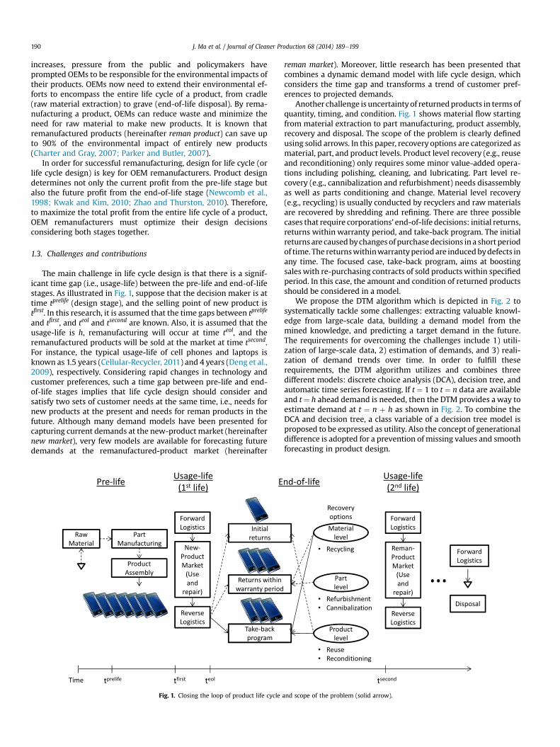
The main challenge in life cycle design is that there is a signif-icant time gap (i.e., usage-life) between the pre-life and end-of-lifestages. As illustrated in Fig. 1, suppose that the decision maker is attime tprelife (design stage), and the selling point of new product istfirst. In this research, it is assumed that the time gaps between tprelife

and tfirst, and teol and tsecond are known. Also, it is assumed that theusage-life is h, remanufacturing will occur at time teol, and theremanufactured products will be sold at the market at time tsecond.For instance, the typical usage-life of cell phones and laptops isknown as 1.5 years (Cellular-Recycler, 2011) and 4 years (Deng et al.,2009), respectively. Considering rapid changes in technology andcustomer preferences, such a time gap between pre-life and end-of-life stages implies that life cycle design should consider andsatisfy two sets of customer needs at the same time, i.e., needs fornew products at the present and needs for reman products in thefuture. Although many demand models have been presented forcapturing current demands at the new-product market (hereinafternew market), very few models are available for forecasting futuredemands at the remanufactured-product market (hereinafter

Fig. 1. Closing the loop of product life cycle

reman market). Moreover, little research has been presented thatcombines a dynamic demand model with life cycle design, whichconsiders the time gap and transforms a trend of customer pref-erences to projected demands.

Another challenge is uncertainty of returnedproducts in termsofquantity, timing, and condition. Fig. 1 shows material flow startingfrom material extraction to part manufacturing, product assembly,recovery and disposal. The scope of the problem is clearly definedusing solid arrows. In this paper, recovery options are categorized asmaterial, part, and product levels. Product level recovery (e.g., reuseand reconditioning) only requires some minor value-added opera-tions including polishing, cleaning, and lubricating. Part level re-covery (e.g., cannibalization and refurbishment) needs disassemblyas well as parts conditioning and change. Material level recovery(e.g., recycling) is usually conducted by recyclers and raw materialsare recovered by shredding and refining. There are three possiblecases that require corporations’ end-of-life decisions: initial returns,returns within warranty period, and take-back program. The initialreturns are causedbychanges of purchasedecisions in a short periodof time. The returnswithinwarrantyperiodare inducedbydefects inany time. The focused case, take-back program, aims at boostingsales with re-purchasing contracts of sold products within specifiedperiod. In this case, the amount and condition of returned productsshould be considered in a model.

We propose the DTM algorithm which is depicted in Fig. 2 tosystematically tackle some challenges: extracting valuable knowl-edge from large-scale data, building a demand model from themined knowledge, and predicting a target demand in the future.The requirements for overcoming the challenges include 1) utili-zation of large-scale data, 2) estimation of demands, and 3) reali-zation of demand trends over time. In order to fulfill theserequirements, the DTM algorithm utilizes and combines threedifferent models: discrete choice analysis (DCA), decision tree, andautomatic time series forecasting. If t ¼ 1 to t ¼ n data are availableand t¼ h ahead demand is needed, then the DTM provides away toestimate demand at t ¼ n þ h as shown in Fig. 2. To combine theDCA and decision tree, a class variable of a decision tree model isproposed to be expressed as utility. Also the concept of generationaldifference is adopted for a prevention of missing values and smoothforecasting in product design.

and scope of the problem (solid arrow).

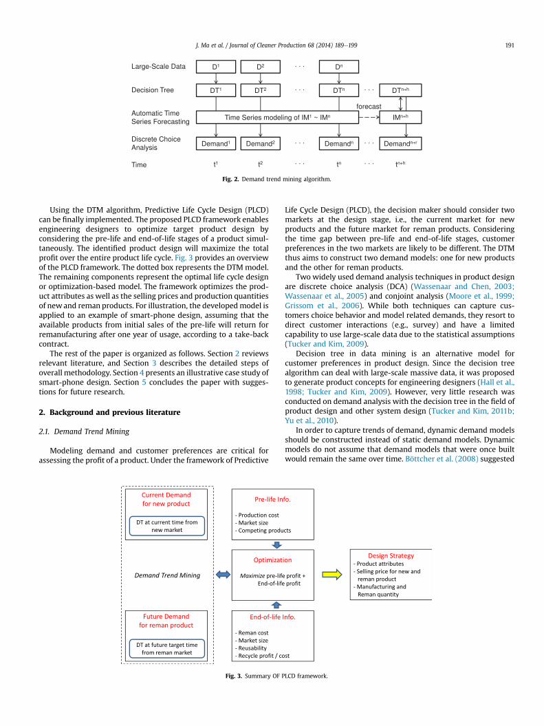
Fig. 2. Demand trend mining algorithm.

J. Ma et al. / Journal of Cleaner Production 68 (2014) 189e199 191

Using the DTM algorithm, Predictive Life Cycle Design (PLCD)can be finally implemented. The proposed PLCD framework enablesengineering designers to optimize target product design byconsidering the pre-life and end-of-life stages of a product simul-taneously. The identified product design will maximize the totalprofit over the entire product life cycle. Fig. 3 provides an overviewof the PLCD framework. The dotted box represents the DTMmodel.The remaining components represent the optimal life cycle designor optimization-based model. The framework optimizes the prod-uct attributes as well as the selling prices and production quantitiesof newand reman products. For illustration, the developedmodel isapplied to an example of smart-phone design, assuming that theavailable products from initial sales of the pre-life will return forremanufacturing after one year of usage, according to a take-backcontract.

The rest of the paper is organized as follows. Section 2 reviewsrelevant literature, and Section 3 describes the detailed steps ofoverall methodology. Section 4 presents an illustrative case study ofsmart-phone design. Section 5 concludes the paper with sugges-tions for future research.

2. Background and previous literature

2.1. Demand Trend Mining

Modeling demand and customer preferences are critical forassessing the profit of a product. Under the framework of Predictive

Fig. 3. Summary OF P

Life Cycle Design (PLCD), the decision maker should consider twomarkets at the design stage, i.e., the current market for newproducts and the future market for reman products. Consideringthe time gap between pre-life and end-of-life stages, customerpreferences in the two markets are likely to be different. The DTMthus aims to construct two demand models: one for new productsand the other for reman products.

Two widely used demand analysis techniques in product designare discrete choice analysis (DCA) (Wassenaar and Chen, 2003;Wassenaar et al., 2005) and conjoint analysis (Moore et al., 1999;Grissom et al., 2006). While both techniques can capture cus-tomers choice behavior and model related demands, they resort todirect customer interactions (e.g., survey) and have a limitedcapability to use large-scale data due to the statistical assumptions(Tucker and Kim, 2009).

Decision tree in data mining is an alternative model forcustomer preferences in product design. Since the decision treealgorithm can deal with large-scale massive data, it was proposedto generate product concepts for engineering designers (Hall et al.,1998; Tucker and Kim, 2009). However, very little research wasconducted on demand analysis with the decision tree in the field ofproduct design and other system design (Tucker and Kim, 2011b;Yu et al., 2010).

In order to capture trends of demand, dynamic demand modelsshould be constructed instead of static demand models. Dynamicmodels do not assume that demand models that were once builtwould remain the same over time. Böttcher et al. (2008) suggested

LCD framework.

J. Ma et al. / Journal of Cleaner Production 68 (2014) 189e199192

that decision tree can be built based on predicted values of inter-estingness measure (IM). IM is a term for “various measuresdevised for evaluating and ranking discovered patterns producedby the data mining process” (McGarry, 2005). To trace the trend ofIMs, a polynomial regression model was utilized. Tucker and Kim(2011b) suggested the adoption of the time series analysis tech-nique, HolteWinters exponential smoothing model, which is amore complex modeling technique with time-variant data. How-ever, there exist different classes of exponential smoothing, whichmeans the HolteWinters model is just one of its family and engi-neering designers should choose right one among them. At thesame time, designers are required to determine many differentparameters and initial states for the HolteWinters model. The DTMalgorithm adopted the Hyndman’s automatic time series fore-casting algorithm (Hyndman et al., 2008; Hyndman and Khandakar,2008). This algorithm includes the automatic optimization processfor model selection, parameter setting, and initial state estimationwith the innovations formulation of state space models.

The proposed DTM combines the merits of aforementionedthree different models: DCA for demandmodeling, decision tree forlarge-scale data, and automatic time series forecasting for trendanalysis. The decision tree algorithm, C4.5, models customer pref-erences from large-scale data, and by formulating a class variable asutility, the resulting decision tree models can estimate marketshares from the DCA, specifically logit choice probability in multi-nomial logit (MNL) model. Automatic time series forecasting pro-vides predicted IMs, and trend reflected demand is estimated fromthe target time decision tree.

Table 1 provides a summary of the MNL and C4.5 (Tucker andKim, 2011b; Tucker et al., 2009). The MNL model starts from arandom utility model where the true utility consists of theobservable utility and the unobservable random part. In the MNL,the random part is assumed as independent and identicallydistributed extreme value, and the choice probability is given bythe logit choice probability. The C4.5 is based on the informationtheory. Entropy, a measure of disorder or complexity, is calculated,and the decision tree is built in the direction of minimizing theentropy.

2.2. Predictive Life Cycle Design

Design for life cycle or life cycle design focuses on the fact thatdecisions made at the design stage affect all phases of a product’slife cycle (i.e., material extraction, manufacturing, usage, and end-of-life recycling and disposal). In many previous studies, it hasbeen emphasized that the design stage determines 70e85% of aproduct’s total life cycle cost and environmental impact (Fixson,2004; Duverlie and Castelain, 1999; Seo et al., 2002). Therefore,life cycle design is aimed at proactively dealing with economic andenvironmental issues during the early design stage when the po-tential for affecting results is the greatest. Since little research has

Table 1Overview Of Mnl and C4.5 (Tucker and Kim, 2011b; Tucker et al., 2009).

MNL

Assumption - Random Utility ModelUnj ¼ Vnj þ enjenj w iid extreme valuej: choice alternativen: decision maker

Choice Probability & Split Criterion - Logit Choice Probability

Pni ¼ expðVniÞPiexpðVnjÞ

Decision maker n choose aover alternative j (i s j)

been conducted for the economic perspective in comparison withthe matured environmental perspective over entire life cycle(Hundal, 2001; Kwak, 2012), only the economic side of productdesign is considered in this paper. However, the economic benefitsfrom the end-of-life stage that are traditionally hidden source ofprofit can lead to environmentally friendly design by consideringend-of-life processes.

Some researchers (Lye et al., 2001; O’Shea, 2002; Holt andBarnes, 2010) have developed a holistic design approach thatconsiders various concerns of all life cycle stages in an integratedmanner. However, a more popular approach has been to developdesign principles for improving a specific life cycle stage. Design forrecovery, design for remanufacturing, design for disassembly, anddesign for recycling are among the principles of life cycle design.Focusing on the end-of-life stage, they seek to identify optimalproduct design to reduce the cost of recovery and/or increase theprofit associated with recovery.

Rose et al. (2000, 2002) suggested a classification scheme forhelping designers predict appropriate recovery strategies for aproduct, so that the designers can redesign products to move to-ward a higher level of reuse. Mangun and Thurston (2002) devel-oped a model for designing a product portfolio that incorporatedpart reuse through refurbishment. Givenmultiplemarket segmentswith varying requirements for environmental impact, productioncost, and reliability, they attempted to determine the optimalproduct design for each segment in order to maximize the totalutility of the portfolio. Kwak and Kim (2010, 2011) introduced aframework for analyzing how product design affects end-of-liferecovery and what architectural characteristics are desirable forhigher recovery profit.

One limitation of these previous methods, however, is that thedesign implications on the pre-life and end-of-life stages have beenconsidered separately. Product design has been optimized for eachof the stages, but not for the stages together due to the lack ofavailable demand forecasting models. By the proposed DTM algo-rithm, both stages now can be considered together. This is why theframework is called Predictive Life Cycle Design. Two exceptions canbe found in Zhao and Thurston (2010) and Kwak and Kim (2013a).Both developed a mathematical model to determine the optimalproduct design that maximizes the profits from both initial salesand end-of-life recovery. They showed that the total profit can bemaximized when both ends of the product life cycle are consideredat the same time. However, the prediction and reflection of demandtrends in the market were not incorporated.

3. Methodology

This section describes detailed steps for the DTM and PLCD.Fig. 4 shows the overall framework of the PLCD which has twocomponents: DTM and optimal life cycle design. Although thegeneral description of the DTM algorithm is described in Figs. 2 and

C4.5

- Information Theory (Information Entropy)EntropyðDÞ ¼ �Pk

i¼1Pi$log2PiD: data setk: number of class variables within the data setPi: probability of class variable i

lternative i

- Gain RatioGain RatioðXÞ ¼ EntropyðDÞ�

Pn

j¼1

jDjjjDj $EntropyðDjÞ

�Pn

j¼1

jDjjjDj $log2

jDj jjDjX : attribute

n : number of outcomes for a given attribute

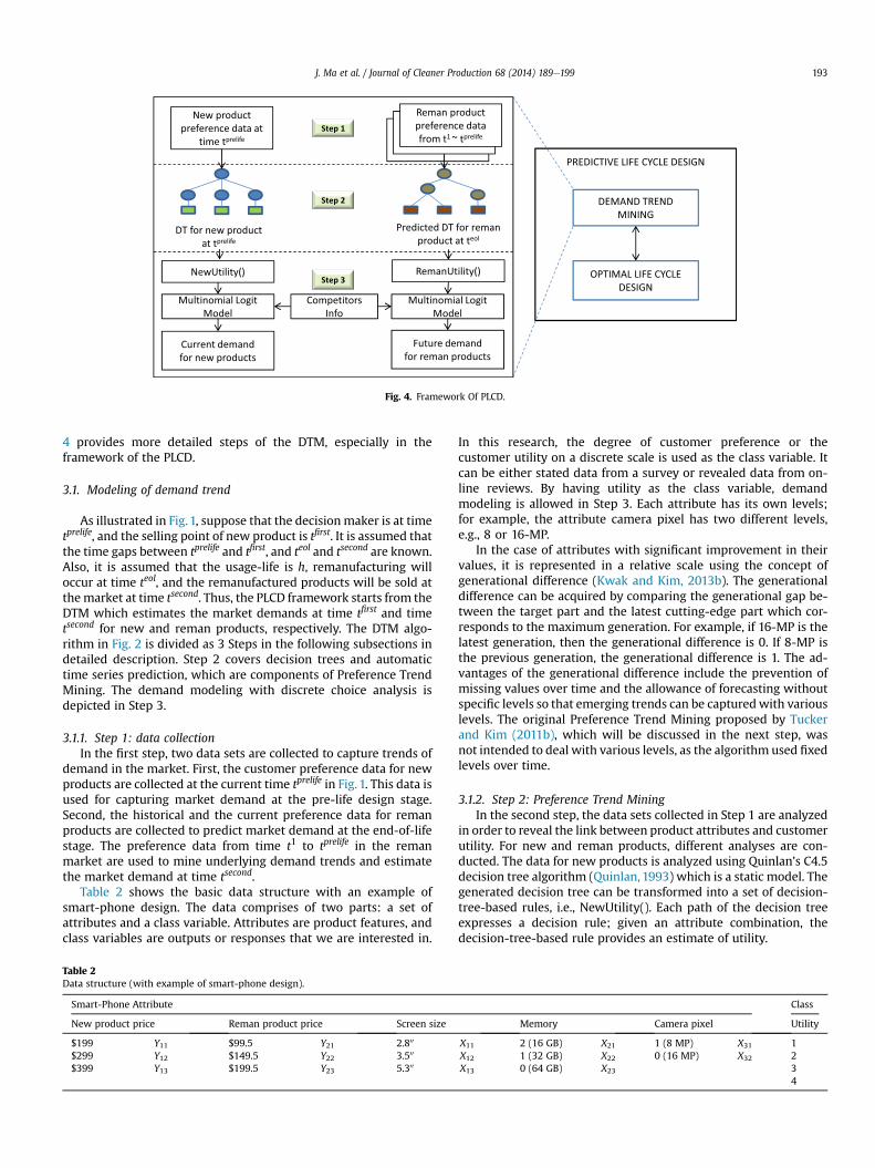
Fig. 4. Framework Of PLCD.

J. Ma et al. / Journal of Cleaner Production 68 (2014) 189e199 193

4 provides more detailed steps of the DTM, especially in theframework of the PLCD.

3.1. Modeling of demand trend

As illustrated in Fig. 1, suppose that the decisionmaker is at timetprelife, and the selling point of new product is tfirst. It is assumed thatthe time gaps between tprelife and tfirst, and teol and tsecond are known.Also, it is assumed that the usage-life is h, remanufacturing willoccur at time teol, and the remanufactured products will be sold atthemarket at time tsecond. Thus, the PLCD framework starts from theDTM which estimates the market demands at time tfirst and timetsecond for new and reman products, respectively. The DTM algo-rithm in Fig. 2 is divided as 3 Steps in the following subsections indetailed description. Step 2 covers decision trees and automatictime series prediction, which are components of Preference TrendMining. The demand modeling with discrete choice analysis isdepicted in Step 3.

3.1.1. Step 1: data collectionIn the first step, two data sets are collected to capture trends of

demand in the market. First, the customer preference data for newproducts are collected at the current time tprelife in Fig. 1. This data isused for capturing market demand at the pre-life design stage.Second, the historical and the current preference data for remanproducts are collected to predict market demand at the end-of-lifestage. The preference data from time t1 to tprelife in the remanmarket are used to mine underlying demand trends and estimatethe market demand at time tsecond.

Table 2 shows the basic data structure with an example ofsmart-phone design. The data comprises of two parts: a set ofattributes and a class variable. Attributes are product features, andclass variables are outputs or responses that we are interested in.

Table 2Data structure (with example of smart-phone design).

Smart-Phone Attribute

New product price Reman product price Screen size

$199 Y11 $99.5 Y21 2.800

$299 Y12 $149.5 Y22 3.500

$399 Y13 $199.5 Y23 5.300

In this research, the degree of customer preference or thecustomer utility on a discrete scale is used as the class variable. Itcan be either stated data from a survey or revealed data from on-line reviews. By having utility as the class variable, demandmodeling is allowed in Step 3. Each attribute has its own levels;for example, the attribute camera pixel has two different levels,e.g., 8 or 16-MP.

In the case of attributes with significant improvement in theirvalues, it is represented in a relative scale using the concept ofgenerational difference (Kwak and Kim, 2013b). The generationaldifference can be acquired by comparing the generational gap be-tween the target part and the latest cutting-edge part which cor-responds to the maximum generation. For example, if 16-MP is thelatest generation, then the generational difference is 0. If 8-MP isthe previous generation, the generational difference is 1. The ad-vantages of the generational difference include the prevention ofmissing values over time and the allowance of forecasting withoutspecific levels so that emerging trends can be capturedwith variouslevels. The original Preference Trend Mining proposed by Tuckerand Kim (2011b), which will be discussed in the next step, wasnot intended to deal with various levels, as the algorithm used fixedlevels over time.

3.1.2. Step 2: Preference Trend MiningIn the second step, the data sets collected in Step 1 are analyzed

in order to reveal the link between product attributes and customerutility. For new and reman products, different analyses are con-ducted. The data for new products is analyzed using Quinlan’s C4.5decision tree algorithm (Quinlan, 1993) which is a static model. Thegenerated decision tree can be transformed into a set of decision-tree-based rules, i.e., NewUtility(). Each path of the decision treeexpresses a decision rule; given an attribute combination, thedecision-tree-based rule provides an estimate of utility.

Class

Memory Camera pixel Utility

X11 2 (16 GB) X21 1 (8 MP) X31 1X12 1 (32 GB) X22 0 (16 MP) X32 2X13 0 (64 GB) X23 3

4

J. Ma et al. / Journal of Cleaner Production 68 (2014) 189e199194

The time series data for reman products is analyzed using therevised Preference Trend Mining (PTM) algorithm adopted byTucker and Kim (2011b). The algorithm generates a predicted de-cision tree for the future time teol, which can provide a set of de-cision rules, i.e., RemanUtility(). Algorithm 1 shows the pseudocode for the PTM. ST is the time series data (from time t1 to tprelife)for reman products and X is the set of attributes. The PTM algorithmis similar to the C4.5 algorithm in that it builds the decision treebased on the interestingness measure (IM). In both algorithms, theattribute with the maximum IM becomes the node for branching.The difference is in how to calculate the IMs.

Unlike the C4.5 using one aggregated data set, the PTM forecaststhe IMs of the future time from the historical time series data. InAlgorithm 1, the PTM starts from finding the IMs of all attributes Xfrom all previous data (line 3). Then, there are processes to predictthe IMs at teol using the IMs from t1 to tprelife and assign the attributewith the maximum IM as the root node of the tree (line 5). Thelevels of the attribute then become branches. For each branch, thesame processes are repeated for remaining attributes; i.e. the PTMchecks which attribute has the maximum IM at teol and iterativelysplits a decision tree until it reaches termination criteria. Afteridentifying all the leaf nodes, the algorithm returns the predicteddecision tree.

Algorithm 1. Preference Trend Mining revised from Tucker andKim (2011b)

1: procedure PTM (ST)2: while Termination criteria are met do3: Find IM(X) for ST and Forecast IM(X) at teol

4: If IM(Xi) ¼ MAX IM(X) at teol

5: Then Xi ¼ root node, Xi levels ¼ branches6: Find IM(X) for ST and Forecast IM(X) at teol given selectedbranches7: If IMðX0

iÞ ¼ MAX IM(X) at teol

8: Then X0i ¼ childnode, X0

i levels ¼ branches9: Repeat 6, 7, 810: end while11: Result class variable ¼ leaf node12: return Predicted decision tree13: end procedure

To apply the PTM algorithm, three issues should be clarified.First, the decision maker should decide the IM to use. The IMs thatare well known and widely used include Shannon’s entropy, giniindex, information gain, and gain ratio. Depending on the data andits characteristics, each measure has its own pros and cons (Harris,2002). In this paper, the gain ratio was selected following the C4.5algorithm although the approach can be generalized with theother IMs.

The second issue is about the forecasting engine for the IMprediction. Hyndman’s exponential smoothing (Hyndman et al.,2008) and the BoxeJenkins model (Box and Jenkins, 1976; Nayloret al., 1972) are among the most popular and widely-usedmethods for time series forecasting. In the Hyndman’s exponen-tial smoothing, the time series data can be decomposed into fourcomponents, i.e., trend, seasonal, cycle, and irregular error. A totalof 30 mathematical models are available, and the best model can beobtained using automatic time series forecasting algorithm(Hyndman et al., 2008; Hyndman and Khandakar, 2008). The Box-Jenkins model is another popular option. It applies an autore-gressive moving average (ARMA) or an autoregressive integratedmoving average (ARIMA) to fit the time series data. Exponentialsmoothing has value in that it is relatively simple and easy to un-derstand though there is no general consensus aboutwhich one has

a better prediction accuracy (Gooijer and Hyndman, 2006; Geurtsand Ibrahim, 1975). In this research, Hyndman’s exponentialsmoothingmodel, specifically the automatic time series forecastingmethod, is chosen as the forecasting engine.

The difference between the Holt-Winters model in the originalPTM (Tucker and Kim, 2011b) and the automatic time series fore-casting (Hyndman et al., 2008, 2002) in the DTM is that the formeris just one of exponential smoothing family and requires many ofuser inputs, but the latter allows automated model selection, andparameters and initial state estimation among 30 different linearand nonlinear models for designers.

Termination criteria in decision-tree generation is anotherimportant issue. If all class variables are distributed homoge-neously and no valid split is found, the process can be stopped. Ifthe leaf node is reached and the class variables are not distributedhomogeneously, the path can be removed or the dominant classvariable over time can be selected.

3.1.3. Step 3: demand modelingThe decision trees obtained in Step 2 provide two sets of deci-

sion rules, NewUtility() and RemanUtility(). The decision rules giveestimates on customer utility that corresponds to a set of designattributes. NewUtility() gives the utility estimates in the currentnew market, and RemanUtility() gives the estimates in the futurereman market.

Once customer utilities for a specific product and its competingproducts are given, it is possible to estimate the market share ofeach of the products. In this research, logit choice probability of themultinomial logit (MNL) model (Train, 2003) is used as shown inEquations (1) and (2), where l and m are the product choicesavailable in the new and reman markets, respectively; Yij is a vectorof binary variables representing price related (Y1j for price of a newproduct, Y2j for price of a reman product) product attributes andtheir levels; Xij is a vector of binary variables representingcomponent related product attributes and their levels; MSnew andMSreman are the sizes of new and reman markets, respectively;Dnew(Y1j,Xij) and Dreman(Y2j,Xij) are market demands for new andreman products, respectively.

Dnew�Y1j; Xij� ¼ expðNewUtiliy

�Y1j; Xij

�Pl

1exp�NewUtiliyl

�Y1j; Xij

��MSnew (1)

Dreman�Y2j; Xij� ¼ exp

�RemanUtiliy

�Y2j; Xij

��Pm

1 exp�RemanUtiliyl

�Y2j; Xij

��MSreman

(2)

3.2. Optimal life cycle design

The optimal life cycle design model is the optimization enginefor the PLCD. Table 3 shows the problem statement of the optimi-zationmodel. With the aim tomaximize the pre-life and end-of-lifeprofits together, the model identifies the optimal product design aswell as optimal production strategies at the pre-life and the end-of-life stages (i.e., the quantities and selling prices of new and remanproducts). The model assumes that the new products sold at timetfirst are all taken back for recovery after h years at time teol. A certainpercentage of the initial selling price, ε$Pnew, is paid for the take-back. It is also assumed that the returned end-of-life products areall recovered by either remanufacturing or recycling. Customerabuse and product reliability can affect the availability of rema-nufacturable products. Based on the product condition, onlyworking products are allowed for remanufacturing. During theremanufacturing operation, no loss in yield or no scrap is assumed.Also, upgrades of parts are not considered. In other words, products

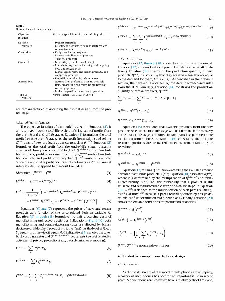
Table 3Optimal life cycle design model.

Objectivefunction

Maximize (pre-life profit þ end-of-life profit)

DecisionVariables

- Product attributes- Quantity of products to be manufactured andremanufactured

Constraints - Design attributes uniqueness- No excess fulfillment of products- Take-back program

Given Info - NewUtility () and RemanUtility ()- Manufacturing, remanufacturing and recyclingcost, and recycle profit

- Market size for new and reman products, andcompeting products

- Reusability or reliability of componentsAssumptions - Accumulated preference data are available

- Remanufacturing and recycling are possiblerecovery options

- No loss in yield in the recovery operationType of

ProblemMixed Integer Non-Linear Problem

J. Ma et al. / Journal of Cleaner Production 68 (2014) 189e199 195

are remanufactured maintaining their initial design from the pre-life stage.

3.2.1. Objective functionThe objective function of the model is given in Equation (3). It

aims to maximize the total life cycle profit, i.e., sum of profits fromthe pre-life and end-of-life stages. Equation (4) formulates the totalprofit from the pre-life stage, i.e., the profit frommaking and sellingQnew units of new products at the current time tprelife. Equation (5)formulates the total profit from the end-of-life stage. It mainlyconsists of three parts: cost of taking back Qtakeback units of end-of-life products, profit from remanufacturing Qreman units of end-of-life products, and profit from recycling Qrecycle units of products.Since the end-of-life profit occurs at the future time teol, an annualinterest rate a is applied to discount the value.

Maximize f prelife þ f eol (3)

f prelife ¼ ðPnew � CnewÞQnew (4)

f eol ¼ 1

ð1þ aÞhh�

� Ctakeback$Qtakeback þ ðPreman$Qreman

� Creman$QremanÞ�þ�Precycle � Crecycle

�Qrecycle

i(5)

Equations (6) and (7) represent the prices of new and remanproducts as a function of the price related decision variable Yij.Equation (8) through (11) formulate the unit processing costs ofmanufacturing andrecoveryactivities. In Equations (8) and (10), bothmanufacturing and remanufacturing costs are affected by binarydecisionvariables, Xij. If product attribute i (i˛I) has the level of j (j˛J),Yij equals 1; otherwise, it equals 0. ü in Equation (9) denotes the take-back cost parameter and Cprivacyprotection represents the cost related toactivities of privacy protection (e.g., data cleaning or scrubbing).

Pnew ¼Xj

Pnew1j $Y1j (6)

Preman ¼Xj

Preman2j $Y2j (7)

Cnew ¼Xi

Xj

Cmanufacturingij $Xij þ Cforwardlogistics (8)

Ctakeback ¼ ε$PnewþCreverselogisticsþCsortingþCprivacyprotection (9)

Creman ¼Xi

Xj

Creconditioningij $Xij þ Cforwardlogistics (10)

Crecycle ¼ Crecycling þ Cforwardlogistics (11)

3.2.2. ConstraintsEquations (12) through (20) show the constraints of the model.

Equation (12) imposes that each product attribute i has an attributelevel j. Equation (13) constrains the production quantity of newproducts, Qnew, in such away that they are always less than or equalto the demand for them, Dnew(Y1j,Xij). As described in the previoussection, the demand is obtained by the decision-tree-based rulesfrom the DTM. Similarly, Equation (14) constrains the productionquantity of reman products, Qreman.Xj

Yij ¼ 1;Xj

Xij ¼ 1; Yij; Xij˛f0; 1g (12)

Qnew � Dnew�Y1j; Xij�

(13)

Qreman � Dreman�Y2j; Xij�

(14)

Equation (15) formulates that available products from the newproducts sales at the first-life stage will be taken back for recoveryat the end-of-life stage. r denotes the take-back loss parameter dueto the customer abuse. Equation (16) constrains that all thereturned products are recovered either by remanufacturing orrecycling.

Qtakeback ¼ r$Qnew (15)

Qtakeback ¼ Qreman þ Qrecycle (16)

Equation (17) refrainsQreman fromexceeding theavailable amountof remanufacturable products, A(teol). Equation (18) estimates A(teol),where it is determined by the multiplication of Qtakeback and rema-nufacturability, d(teol), i.e., the probability that a product is stillreusable and remanufacturable at the end-of-life stage. In Equation(19), d(teol) is defined as the multiplication of each part’s reliability,gj(teol), at time teol. Because a part’s reliability differs by design de-cisions, d(teol) is formulated as a function of Xij. Finally, Equation (20)shows the variable conditions for production quantities.

Qreman � A�teol

�(17)

A�teol

�¼ Qnew$d

�teol

�(18)

d�teol

�¼

Yi

0@X

j

gj

�teol

�$Xij

1A (19)

Qnew;Qreman˛nonnegative integer (20)

4. Illustrative example: smart-phone design

4.1. Overview

As the waste stream of discarded mobile phones grows rapidly,recovery of used phones has become an important issue in recentyears. Mobile phones are known to have a relatively short life cycle,

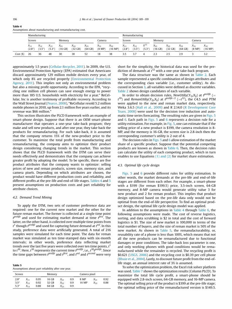
Table 4Assumptions about manufacturing and remanufacturing cost.

Manufacturing Remanufacturing

Screen Memory Camera Screen Memory Camera

X11

(2.8ʺ)X12

(3.5ʺ)X13

(5.3ʺ)X21

(16 GB)X22

(32 GB)X23

(64 GB)X31

(8 MP)X32

(16 MP)X11

(2.8ʺ)X12

(3.5ʺ)X13

(5.3ʺ)X21

(16 GB)X22

(32 GB)X23

(64 GB)X31

(8 MP)X32

(16 MP)

Cost ($) 26 36 48 30 38 52 18 38 3.5 3.7 4 2.3 2.5 2.9 3 3.2

J. Ma et al. / Journal of Cleaner Production 68 (2014) 189e199196

approximately 1.5 years (Cellular-Recycler, 2011). In 2009, the U.S.Environmental Protection Agency (EPA) estimated that Americansdiscard approximately 129 million mobile devices every year, ofwhich only 8% are recycled properly (Environmental ProtectionAgency, 2011). This implies not only an environmental problembut also a missing profit opportunity. According to the EPA, “recy-cling one million cell phones can save enough energy to powermore than 185 U.S. households with electricity for a year.” ReCel-lular, Inc is another testimony of profitable recovery. According totheWall Street Journal (Pearce, 2008), “ReCellular resold 5.2millionmobile phones in 2010, up from 2.1 million five years earlier, and itsrevenue was $66 million.”

This section illustrates the PLCD framework with an example ofsmart-phone design. Suppose that there is an OEM smart-phonemanufacturer that operates a one-year take-back program; theymake and sell new products, and after one year, they take back theproducts for remanufacturing. For such take-back, it is assumedthat the company returns 15% of the new-product price to thecustomer. To maximize the total profit from manufacturing andremanufacturing, the company aims to optimize their productdesign considering changing trends in the market. This sectionshows that the PLCD framework with the DTM can serve theirneeds effectively and demonstrates that the company can achievegreater profit by adopting the model. To be specific, there are fiveproduct attributes that the company wants to optimize: sellingprices of new and reman products, screen size, memory size, andcamera pixels. Depending on which attributes are chosen, theproduct would have different production costs and reliability, anddifferent profits at the pre-life and end-of-life stages. Tables 4 and 5present assumptions on production costs and part reliability forattribute choices.

4.2. Demand Trend Mining

To apply the DTM, two sets of customer preference data arerequired: one for the current new market and the other for thefuture reman market. The former is collected at a single time pointtprelife and used for estimating market demand at time tfirst. Thelatter, on the other hand, is collected overmultiple time points fromt1 though tprelife and used for capturing future demand at teol. In thisstudy, preference data were artificially generated. A total of 216samples were simulated for each time point. The data for remanmarket was simulated as ten time-stamped data with six-monthintervals; in other words, preference data reflecting markettrends over the last five years were collected over ten time points, t1

to t10. Here, t10 represents the current time tprelife, i.e., t10tprelife. Sincethe time gaps between tprelife and tfirst, and teol and tsecond were very

Table 5Assumptions about part reliability after one year.

Screen Memory Camera pixel

2.800 X11 0.95 16 GB X21 0.9 8 MP X31 0.923.500 X12 0.92 32 GB X22 0.9 16 MP X32 0.885.300 X13 0.88 64 GB X23 0.9

short for the simplicity, the historical data was used for the pre-diction of demands at t12 with a one-year take-back program.

The data structure was the same as shown in Table 2. Eachsample represented a specific combination of design attributes andthe corresponding class variable (i.e., customer utility). As dis-cussed in Section 3, all variables were defined as discrete variables.Table 2 shows design candidates of each variable.

In order to obtain decision rules, NewUtiliy(Y1j,Xij) at tprelife (¼t10) and RemanUtiliy(Y2j,Xij) at tprelifeþ2 (¼t12), the C4.5 and PTMwere applied to the new and reman market data, respectively.Weka 3.6.5 (Hall et al., 2009) and R 2.14.0 (R Development CoreTeam, 2008) were used for the decision tree induction and auto-matic time series forecasting. The resulting rules are given in Figs. 5and 6. Each path in Figs. 5 and 6 represents a decision rule for autility estimation. For example, in Fig. 5, one can estimate that if theselling price of a new product is $199, the camera resolution is 8-MP, and the memory is 16-GB, the screen size is 2.8-inch then thecorresponding customer’s utility is 2 out of 4.

The decision rules in Figs. 5 and 6 allow estimation of themarketshare of a specific product. Suppose that the potential competingproducts are known as shown in Table 6. Then, the decision rulescan calculate the utility of each competing product, which in turnenables to use Equations (1) and (2) for market share estimation.

4.3. Optimal life cycle design

Figs. 5 and 6 provide different rules for utility estimation. Inother words, the market demands at the pre-life and end-of-lifestages are different from each other. For example, a smart-phonewith a $199 (for reman $199.5) price, 3.5-inch screen, 64-GBmemory, and 8-MP camera would generate utility value 3 fornew product and 2 for reman product. This implies that productdesign optimized based on the pre-life data only would not beoptimal from the end-of-life perspective. To find an optimal prod-uct design, the optimal life cycle design model was applied.

In addition to the assumptions in Table 4 through Table 6, thefollowing assumptions were made. The cost of reverse logistics,sorting, and data scrubbing is $2 in total and the cost of forwardlogistics is $1. The size of new market is 100,000 in terms of thetotal number of buyers, and the size of reman market is 50% of thenew market. As shown in Table 5, the remanufacturability, or,reusability rate of a phone is less than 100%, which means that notall the new products can be remanufactured due to functionaldamages or poor conditions. The take-back loss parameter is one,and only working phones with good conditions would be rema-nufactured while the remainder is recycled. The recycling profit is$0.621 (USGS, 2006) and the recycling cost is $0.39 per cell phone(Bhuie et al., 2004). Lastly, to discount future profit from the end-of-life stage, an annual interest rate of 3% is assumed.

To solve the optimization problem, the Excel risk solver platformwas used. Table 7 shows the optimization results (Column PLCD). Tomaximize the total life cycle profit, a smart-phone should beequipped with 2.8-inch screen, 64-GB memory, and 16-MP camera.The optimal selling price of the product is $399 at the pre-life stage;the optimal selling price of the remanufactured version is $149.5.

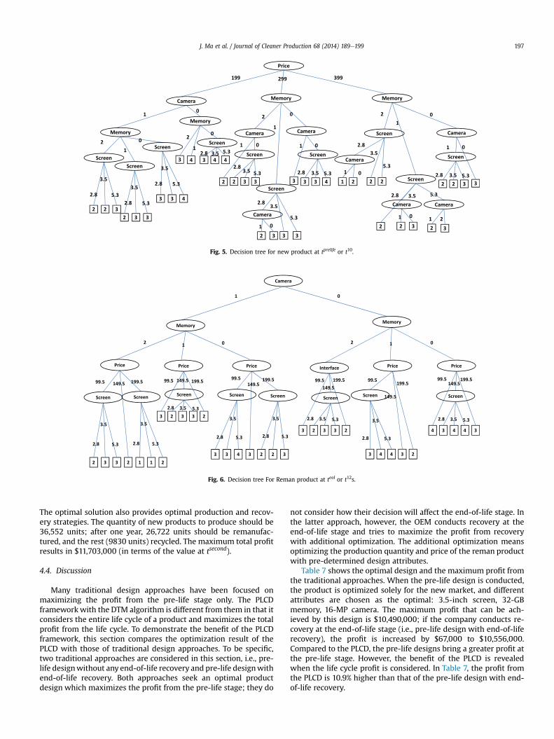
Fig. 5. Decision tree for new product at tprelife or t10.

Fig. 6. Decision tree For Reman product at teol or t12s.

J. Ma et al. / Journal of Cleaner Production 68 (2014) 189e199 197

The optimal solution also provides optimal production and recov-ery strategies. The quantity of new products to produce should be36,552 units; after one year, 26,722 units should be remanufac-tured, and the rest (9830 units) recycled. The maximum total profitresults in $11,703,000 (in terms of the value at tsecond).

4.4. Discussion

Many traditional design approaches have been focused onmaximizing the profit from the pre-life stage only. The PLCDframeworkwith the DTM algorithm is different from them in that itconsiders the entire life cycle of a product and maximizes the totalprofit from the life cycle. To demonstrate the benefit of the PLCDframework, this section compares the optimization result of thePLCD with those of traditional design approaches. To be specific,two traditional approaches are considered in this section, i.e., pre-life designwithout any end-of-life recovery and pre-life designwithend-of-life recovery. Both approaches seek an optimal productdesign which maximizes the profit from the pre-life stage; they do

not consider how their decision will affect the end-of-life stage. Inthe latter approach, however, the OEM conducts recovery at theend-of-life stage and tries to maximize the profit from recoverywith additional optimization. The additional optimization meansoptimizing the production quantity and price of the reman productwith pre-determined design attributes.

Table 7 shows the optimal design and the maximum profit fromthe traditional approaches. When the pre-life design is conducted,the product is optimized solely for the new market, and differentattributes are chosen as the optimal: 3.5-inch screen, 32-GBmemory, 16-MP camera. The maximum profit that can be ach-ieved by this design is $10,490,000; if the company conducts re-covery at the end-of-life stage (i.e., pre-life design with end-of-liferecovery), the profit is increased by $67,000 to $10,556,000.Compared to the PLCD, the pre-life designs bring a greater profit atthe pre-life stage. However, the benefit of the PLCD is revealedwhen the life cycle profit is considered. In Table 7, the profit fromthe PLCD is 10.9% higher than that of the pre-life design with end-of-life recovery.

Table 6Assumptions about competitors information.

High spec product Mid spec product Low spec product

Attributes New price Reman price Screen Memory Camera New price Reman price Screen Memory Camera New price Reman price Screen Memory Camera

Y13 Y23 X13 X23 X32 Y12 Y22 X12 X22 X31 Y11 Y21 X11 X21 X31

New utility3 2 2

Reman utility3 3 2

Table 7Comparative result between PLCD and pre-LIFE design.

PLCD Pre-lifedesign

Pre-life design(þend-of-lifelater)

Total profit [$] 11,703,000 10,490,000 10,557,000Profit for pre-life [$] 10,344,000 10,490,000 10,490,000Profit for end-of-life [$] 1,359,000 e 67,000Product attributes New product

price [$]399 399 399

Reman productprice [$]

149.5 e 99.5

Screen Size [inch] 2.8 3.5 3.5Memory [GB] 64 32 32Camera Pixel [MP] 16 16 16

Quantity of reman product [EA] 26,722 0 26,722Quantity of recycled product [EA] 9830 0 9830New product utility 3 3 3Reman product utility 4 e 4

J. Ma et al. / Journal of Cleaner Production 68 (2014) 189e199198

Previously, the size of the reman market was assumed to be halfthe size of the new market or MSreman ¼ 0.5*MSnew. However, asreported by Pearce (2008) and Cellular-Recycler (2011), the remanmarket is expected to growmore in the future. To see the effect of anincreasing size of remanmarket and validate the outcome in Table 7,a sensitivity analysis is conducted. In Fig. 7, b denotes the ratio ofMSreman to MSnew. For both PLCD and pre-life design (with recovery)models, the sensitivity analysis examined how the maximumachievable profit changes as b increases. A different selection ofdesign attributes and consequent demands and amounts of rema-nufacturable products (Dreman and A) are attributed for differentgaps in the graph. If b ¼ 0, there are no market or demands for thereman products, and no remanufacturing is conducted; if b ¼ 1, thesize of the reman market is the same as the new market. Whenb ¼ 0, the optimizer will determine the optimal design attributesonly from the pre-life stage for bothmodels, whichwill generate the

Fig. 7. Sensitivity analysis OF Reman market size ratio.

same design attributes with the total profit of $8,300,000. Whenb> 0, it is expected that the total profit from the PLCD framework isgreater than that of the pre-life model except the case of selectingthe same design attributes. The results in Fig. 7 show that bothmodels choose all different designs when b > 0. When b ¼ 0.6, theslops of the both models are changed since the upper bound ischanged from Dreman to A (Equations (13) and (17)). When b ¼ 0.7,both models select different designs from the previous ones. Forb¼ 0.8 and b¼ 0.9, the upper bounds are changed again, and finallywhen b ¼ 1, the optimal design is changed for the PLCD. In theillustration example, when b ¼ 0.9, the profit difference is maxi-mized. The results reaffirm that the PLCD framework with the DTMalgorithm is always better than the traditional pre-life design,although the magnitude of the benefit changes depending upon b.

5. Conclusion and future work

This paper proposed a new demand modeling technique, datatrend mining (DTM), for product design analytics. The first contri-bution is the development of the DTM algorithm. In order to cap-ture hidden and upcoming trends of demand, the algorithmcombines three different models: decision tree for large-scale data,discrete choice analysis for demand modeling, and automatic timeseries forecasting for trend analysis. The DTM algorithm dynami-cally reveals design attribute pattern that affects demands. Thesecond contribution is the new design framework, predictive lifecycle design (PLCD), which connects the DTM and data-drivenproduct design. The optimization-based model enables a com-pany to optimize its product design by considering the pre-life andend-of-life stages of a product simultaneously. The DTM modelinteracts with the optimization-based model to maximize the totalprofit of a product. The smart-phone case study demonstrated thatthere is a hidden source of opportunity for profit and the PLCDframework can help utilize this opportunity. Moreover, the sensi-tivity analysis reaffirmed that the life cycle design is more prefer-able than the traditional design method.

The current PLCD framework considers/optimizes two consec-utive life cycles of a single product. In the future, the model can beextended to accommodate multiple life cycles and multiple prod-ucts. The current DTM algorithm allows discrete attributes andclass variables only, which should be extended to process contin-uous attributes and class variables. Also, in reality, it is possible thata product evolves with new attributes. Future work will alsoinclude incorporating emerging attributes into the DTM. Textmining (Tucker and Kim, 2011a; Rai, 2012) and sentiment mining(Stone and Choi, 2013) techniques in the domain of product designcan be candidates for the management of dynamic attribute sets.On-line review data is a promising source that can provide not onlycustomer preferences but also important emerging attributes.

Acknowledgments

The work presented in this paper is supported by the NationalScience Foundation under Award No. CMMI-0953021. Any

J. Ma et al. / Journal of Cleaner Production 68 (2014) 189e199 199

opinions, findings and conclusions or recommendations expressedin this publication are those of the authors and do not necessarilyreflect the views of the National Science Foundation.

References

Bhuie, A., Ogunseitan, O., Saphores, J.D., Shapiro, A., 2004. Environmental andeconomic trade-offs in consumer electronic products recycling: a case study ofcell phones and computers. In: Electronics and the Environment, 2004. Con-ference Record. 2004 IEEE International Symposium on, pp. 74e79.

Böttcher, M., Spott, M., Kruse, R., 2008. Predicting future decision trees fromevolving data. In: Proceedings of ICDM ’08, pp. 33e42.

Box, G.E.P., Jenkins, G., 1976. Time Series Analysis, Forecasting and Control. Holden-Day, Incorporated.

Cellular-Recycler, 2011. Sustainability within the Used Cellular Phone Industry.Report. Cellular Recycler. http://www.cellularrecycler.com/wp/wp-content/uploads/2011/01/CR-Sustainability-Report.pdf.

Charter, M., Gray, C., 2007. Remanufacturing and Product Design: Designing for the7th Generation. Centre for Sustainable Design. Report.

Deng, L., Williams, E., Babbitt, C., 2009. Hybrid life cycle assessment of energy use inlaptop computer manufacturing. In: Sustainable Systems and Technology, 2009.ISSST ’09. IEEE International Symposium.

Duverlie, P., Castelain, J.M., 1999. Cost estimation during design step: parametricmethod versus case based reasoning method. Int. J. Adv. Manuf. Technol. 15,895e906.

Environmental Protection Agency, 2011. Electronics Waste Management in theUnited States through 2009. EPA, U.S. Report EPA 530-R-11-002.

Fixson, S.K., 2004. Assessing product architecture costing: product life cycles,allocation rules, and cost models. In: ASME International Design EngineeringTechnical Conferences and Computers and Information in Engineering Confer-ence (IDETC/CIE2004), Salt Lake City, USA. DETC2004-57458.

Geurts, M.D., Ibrahim, I.B., 1975. Comparing the box-jenkins approach with theexponentially smoothed forecasting model application to Hawaii tourists.J. Mark. Res. 12, 182e188.

Gooijer, J.G.D., Hyndman, R.J., 2006. 25 years of time series forecasting. Int. J.Forecast. 22, 443e473.

Grissom, M., Belegundu, A., Rangaswamy, A., Koopmann, G., 2006. Conjoint-anal-ysis-based multiattribute optimization: application in acoustical design. Struct.Multidiscip. Optim. 31, 8e16.

Hall, L.O., Chawla, N., Bowyer, K.W., 1998. Decision tree learning on very large datasets. In: In IEEE Conference on Systems, Man and Cybernetics, pp. 2579e2584.

Hall, M., Frank, E., Holmes, G., Pfahringer, B., Reutemann, P., Witten, I.H., 2009. Theweka data mining software: an update. SIGKDD Explor. Newsl. 11, 10e18.

Harris, E., 2002. Information gain versus gain ratio: a study of split method biases.In: ISAIM.

Holt, R., Barnes, C., 2010. Towards an integrated approach to design for x: an agendafor decision-based dfx research. Res. Eng. Des. 21, 123e136.

Hucal, M., 2008. Product recycling creates multiple lives for caterpillar machines.Mag. Peoriamagazines. http://www.peoriamagazines.com/ibi/2008/sep/product-recycling-creates-multiple-lives-caterpillar-machines.

Hundal, M., 2001. Mechanical Life Cycle Handbook: Good Environmental Designand Manufacturing. In: Mechanical Engineering. Marcel Dekker.

Hyndman, R., Koehler, A., Ord, J.K., Snyder, R., 2008. Forecasting with ExponentialSmoothing: the State Space Approach. Springer-Verlag, Berlin Heidelberg.

Hyndman, R.J., Khandakar, Y., 2008. Automatic time series forecasting: the forecastpackage for r. J. Stat. Softw. 27 (3), 1e22.

Hyndman, R.J., Koehler, A.B., Snyder, R.D., Grose, S., 2002. A state space frameworkfor automatic forecasting using exponential smoothing methods. Int. J. Forecast.18, 439e454.

King, A., Miemczyk, J., Bufton, D., 2006. Photocopier remanufacturing at xerox UK adescription of the process and consideration of future policy issues. In:Brissaud, D., Tichkiewitch, S., Zwolinski, P. (Eds.), Innovation in Life Cycle En-gineering and Sustainable Development. Springer, Netherlands, pp. 173e186.

Kwak, M., 2012. green Profit Design For Lifecycle. Ph.D. thesis. University of Illinoisat Urbana-Champaign.

Kwak, M., Kim, H.M., 2010. Evaluating end-of-life recovery profit by a simultaneousconsideration of product design and recovery network design. J. Mech. Des. 132,071001.

Kwak, M., Kim, H.M., 2011. Assessing product family design from an end-of-lifeperspective. Eng. Optim. 43, 233e255.

Kwak, M., Kim, H.M., 2013a. Design for lifecycle profit with a simultaneousconsideration of initial manufacturing and end-of-life remanufacturing. Eng.Optim. 135.

Kwak, M., Kim, H.M., 2013b. Market positioning of remanufactured products withoptimal planning for part upgrades. J. Mech. Des. 135.

Labrinidis, A., Jagadish, H.V., 2012. Challenges and opportunities with big data. Proc.VLDB Endow. 5, 2032e2033.

Lund, R.T., 1984. Remanufacturing: the Experience of the United States and Impli-cations for Developing Countries. World Bank, Washington, D.C., U.S.A.

Lye, S.W., Lee, S.G., Khoo, M.K., 2001. A design methodology for the strategicassessment of a product’s eco-efficiency. Int. J. Prod. Res. 39, 2453e2474.

Mangun, D., Thurston, D., 2002. Incorporating component reuse, remanufacture,and recycle into product portfolio design. Eng. Manag. IEEE Trans. 49, 479e490.

McGarry, K., 2005. A survey of interestingness measures for knowledge discovery.Knowl. Eng. Rev. 20, 39e61.

Moore, W.L., Louviere, J.J., Verma, R., 1999. Using conjoint analysis to help designproduct platforms. J. Prod. Innov. Manag. 16, 27e39.

Naylor, T.H., Seaks, T.G., Wichern, D.W., 1972. BoxeJenkins methods: an alternativeto econometric models. Int. Stat. Rev./Rev. Int. Stat. 40, 123e137.

Newcomb, P.J., Bras, B., Rosen, D.W., 1998. Implications of modularity on productdesign for the life cycle. J. Mech. Des. 120, 483e490.

O’Shea, M., 2002. Design for environment in conceptual product design a decisionmodel to reflect environmental issues of all life-cycle phases. J. Sustain. Prod.Des. 2, 11e28.

Parker, D., Butler, P., 2007. An Introduction to Remanufacturing. Report. Centre forRemanufacturing and Reuse.

Pearce, J.A., 2008. In with the old. Mag. Wall Str. J. http://online.wsj.com/news/articles/SB122427020019745211.

Quinlan, J., 1993. C4.5: Programs for Machine Learning. In: Morgan Kaufmann Seriesin Machine Learning. Morgan Kaufmann Publishers.

R Development Core Team, 2008. R: a Language and Environment for StatisticalComputing. R Foundation for Statistical Computing, Vienna, Austria, ISBN 3-900051-07-0.

Rai, R., 2012. Identifying key product attributes and their importance levels fromonline customer reviews. In: ASME International Design Engineering TechnicalConferences and Computers and Information in Engineering Conference(IDETC/CIE2012), Chicago, USA. DETC2012-70493.

Rose, C., Ishii, K., Stevels, A., 2002. Influencing design to improve product end-of-lifestage. Res. Eng. Des. 13, 83e93.

Rose, C., Stevels, A., Ishii, K., 2000. A new approach to end-of-life design advisor(ELDA). In: Electronics and the Environment, 2000. ISEE 2000. Proceedings ofthe 2000 IEEE International Symposium on, pp. 99e104.

Seo, K., Park, J., Jang, D., Wallace, D., 2002. Approximate estimation of the productlife cycle cost using artificial neural networks in conceptual design. Int. J. Adv.Manuf. Technol. 19, 461e471.

Stone, T., Choi, S.K., 2013. Extracting consumer preference from user-generatedcontent sources using classification. In: ASME International Design Engineer-ing Technical Conferences and Computers and Information in EngineeringConference (IDETC/CIE2013), Portland, USA. DETC2013-13228.

Train, K., 2003. Discrete Choice Methods with Simulation. Discrete Choice Methodswith Simulation. Cambridge University Press.

Tucker, C., Hoyle, C., Kim, H.M., Chen, W., 2009. A comparative study of data-intensive demand modeling techniques in relation to product design anddevelopment. In: Proceedings of the ASME Design Engineering Technical Con-ferences, San Diego, CA, USA. DETC2009-87049.

Tucker, C., Kim, H.M., 2008. Optimal product portfolio formulation by mergingpredictive data mining with multilevel optimization. J. Mech. Des. 130, 041103.

Tucker, C., Kim, H.M., 2011a. Predicting emerging product design trend by miningpublicly available customer review data. In: Proceedings of International Con-ference on Engineering Design, Copenhagen, Denmark, pp. 43e52.

Tucker, C., Kim, H.M., 2011b. Trend mining for predictive product design. J. Mech.Des. 133, 111008.

Tucker, C.S., Kim, H.M., 2009. Data-driven decision tree classification for productportfolio design optimization. J. Comput. Inform. Sci. Eng. 9.

USGS, 2006. Recycled Cell Phones e a Treasure Trove of Valuable Metals. U.S.Geological Survey. Fact Sheet 2006-3097. Http://pubs.usgs.gov/fs/2006/3097/fs2006-3097.pdf.

Van Horn, D., Olewnik, A., Lewis, K., 2012. Design analytics: capturing, under-standing and meeting customer needs using big data. In: ASME InternationalDesign Engineering Technical Conferences and Computers and Information inEngineering Conference (IDETC/CIE2012), Chicago, USA. DETC2012-71038.

Wassenaar, H.J., Chen, W., 2003. An approach to decision-based designwith discretechoice analysis for demand modeling. J. Mech. Des. 125, 490e497.

Wassenaar, H.J., Chen, W., Cheng, J., Sudjianto, A., 2005. Enhancing discrete choicedemand modeling for decision-based design. J. Mech. Des. 127, 514e523.

Yu, Z., Haghighat, F., Fung, B.C., Yoshino, H., 2010. A decision tree method forbuilding energy demand modeling. Energy Build. 42, 1637e1646.

Zhao, Y., Thurston, D., 2010. Integrating end-of-life and initial profit considerationsin product life cycle design. In: ASME International Design Engineering Tech-nical Conferences and Computers and Information in Engineering Conference(IDETC/CIE2010), Montreal, Quebec, Canada. DETC2010-28830.