DEEP-wind Jan2012 - DTU Wind - SINTEF · 21 Risø DTU However, simulations can also be sensitive...
38
Presented by Hans E. Jørgensen Head of meteorology program DTU Wind Energy Work done by Andrea N. Hahmann, Alfredo Penaz , Mark Kelly, Søren Ott, Sven Erik Gryning, Gunnar Larsen January 2012: DTU Wind Energy Mesoscale modeling applied to wind energy offshore at DTU Wind Energy Extremes Tall profiles & Ressources wake investigations
Transcript of DEEP-wind Jan2012 - DTU Wind - SINTEF · 21 Risø DTU However, simulations can also be sensitive...
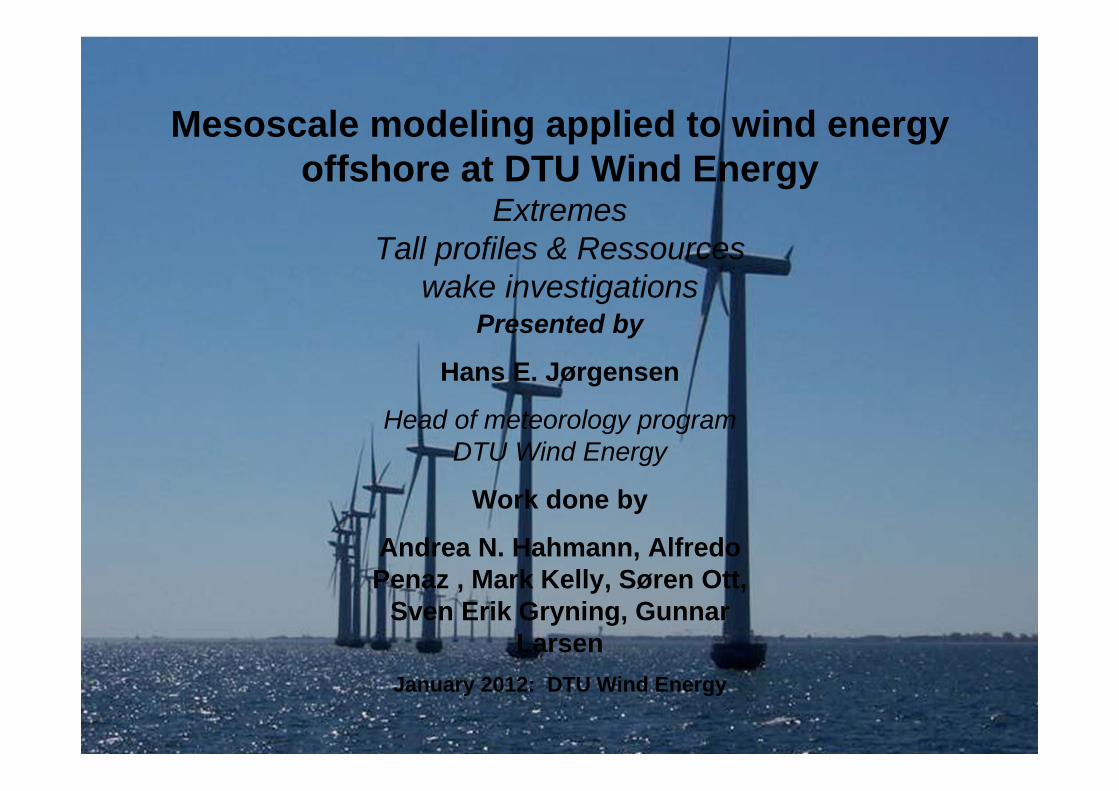
Presented by
Hans E. Jørgensen
Head of meteorology program DTU Wind Energy
Work done by
Andrea N. Hahmann, Alfredo Penaz , Mark Kelly, Søren Ott,
Sven Erik Gryning, Gunnar Larsen
January 2012: DTU Wind Energy
Mesoscale modeling applied to wind energy offshore at DTU Wind Energy
ExtremesTall profiles & Ressources
wake investigations
2 Risø DTU
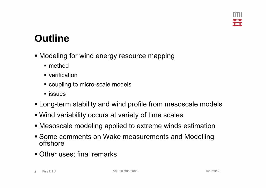
OutlineModeling for wind energy resource mapping method verification coupling to micro-scale models issues
Long-term stability and wind profile from mesoscale modelsWind variability occurs at variety of time scalesMesoscale modeling applied to extreme winds estimation Some comments on Wake measurements and Modelling
offshoreOther uses; final remarks
1/25/2012Andrea Hahmann
3 Risø DTU, Technical University of Denmark
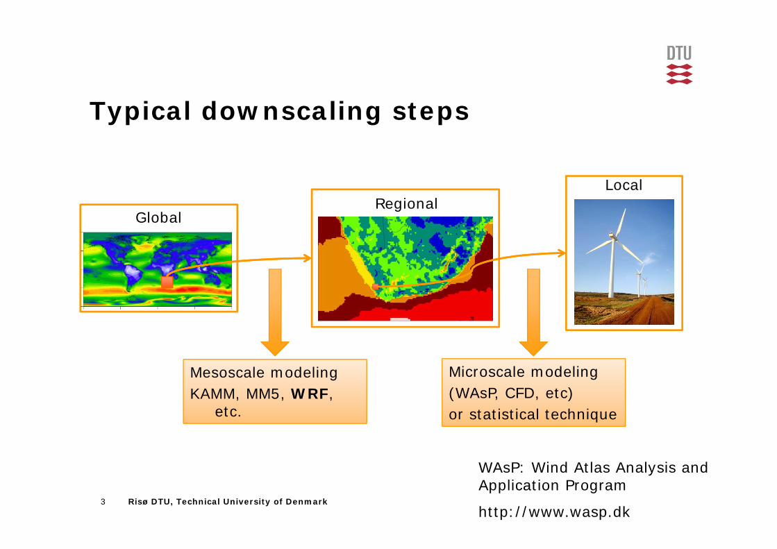
Typical downscaling steps
G
Global
Local
Global wind resources
Regional
Mesoscale modelingKAMM, MM5, WRF,
etc.
Microscale modeling(WAsP, CFD, etc)or statistical technique
WAsP: Wind Atlas Analysis and Application Program
http://www.wasp.dk

4 Risø DTU, Technical University of Denmark
Dynamical downscaling for wind energy resource estimation
For estimating wind energy resources, mesoscale model simulations are:
Not weather forecasting, spin-up may be an issue
Not regional climate simulations, model drift may be an issue
For this application:
We “trust” the large-scale reanalysis that drives the downscaling
We need to resolve smaller scales not present in the reanalysis
global model(reanalysis)
mesoscale model
von Storch et al (2000)

Risø DTU, Technical University of Denmark
Simple/Fast/Cheap Complex/Slow/Expensive
Risø Wind Atlas
Interpolation Statistical-dynamical
Fully dynamical
wind classes from large
pressure field
wind profiles atmos stab.
terrain elevationsurface roughness
wind maps for eachwind class wind resource map
Mes
osca
leM
odel
Mes
osca
leM
odel
+ frequency distributions of wind classes
Downscaling from large-scale toMesoscale (statistical method)
Risø DTU, Technical University of Denmark
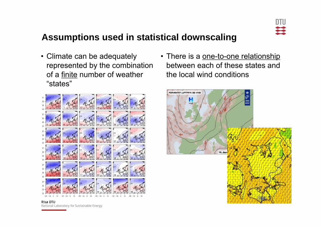
Assumptions used in statistical downscaling
• Climate can be adequately represented by the combination of a finite number of weather “states”
• There is a one-to-one relationship between each of these states and the local wind conditions
7 Risø DTU
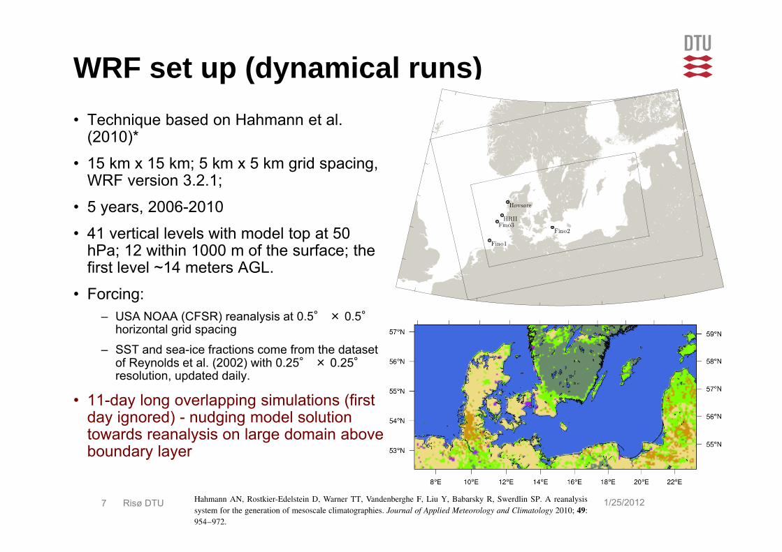
WRF set up (dynamical runs)• Technique based on Hahmann et al.
(2010)*
• 15 km x 15 km; 5 km x 5 km grid spacing, WRF version 3.2.1;
• 5 years, 2006-2010
• 41 vertical levels with model top at 50 hPa; 12 within 1000 m of the surface; the first level ~14 meters AGL.
• Forcing:– USA NOAA (CFSR) reanalysis at 0.5° × 0.5°
horizontal grid spacing
– SST and sea-ice fractions come from the dataset of Reynolds et al. (2002) with 0.25° × 0.25°resolution, updated daily.
• 11-day long overlapping simulations (first day ignored) - nudging model solution towards reanalysis on large domain above boundary layer
1/25/2012
8 Risø DTU, Technical University of Denmark
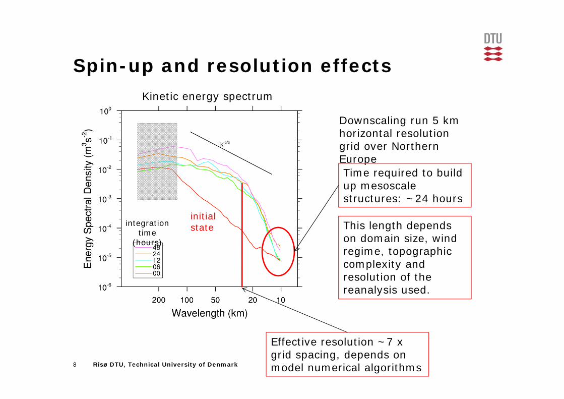
Spin-up and resolution effects
Downscaling run 5 km horizontal resolution grid over Northern EuropeTime required to build up mesoscale structures: ~24 hours
Effective resolution ~7 x grid spacing, depends on model numerical algorithms
initial state
Kinetic energy spectrum
integration time
(hours)
This length depends on domain size, wind regime, topographic complexity and resolution of the reanalysis used.
9 Risø DTU
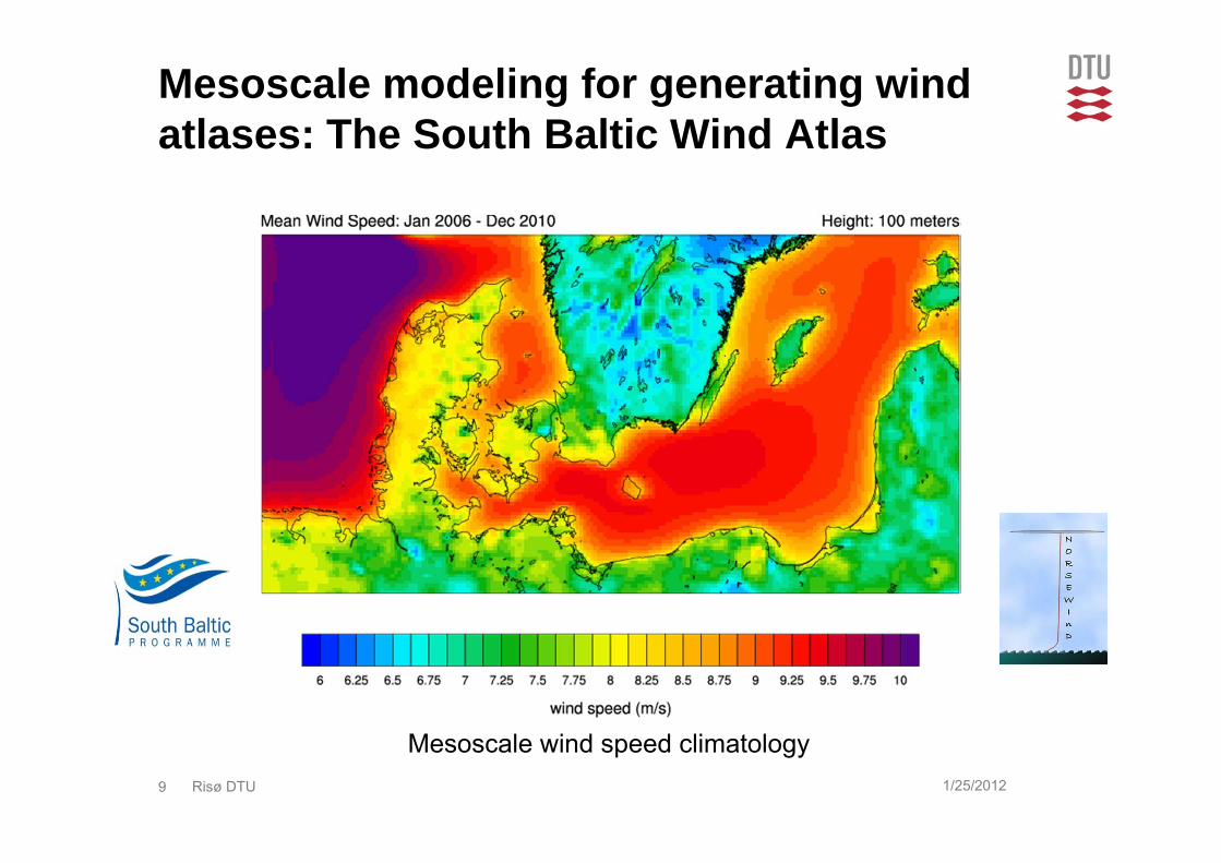
Mesoscale modeling for generating wind atlases: The South Baltic Wind Atlas
1/25/2012
Mesoscale wind speed climatology
10 Risø DTU
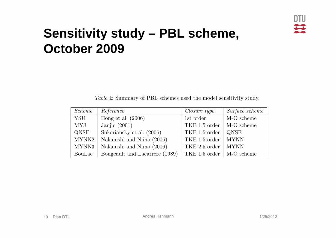
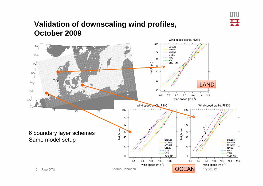
Sensitivity study – PBL scheme, October 2009
1/25/2012Andrea Hahmann
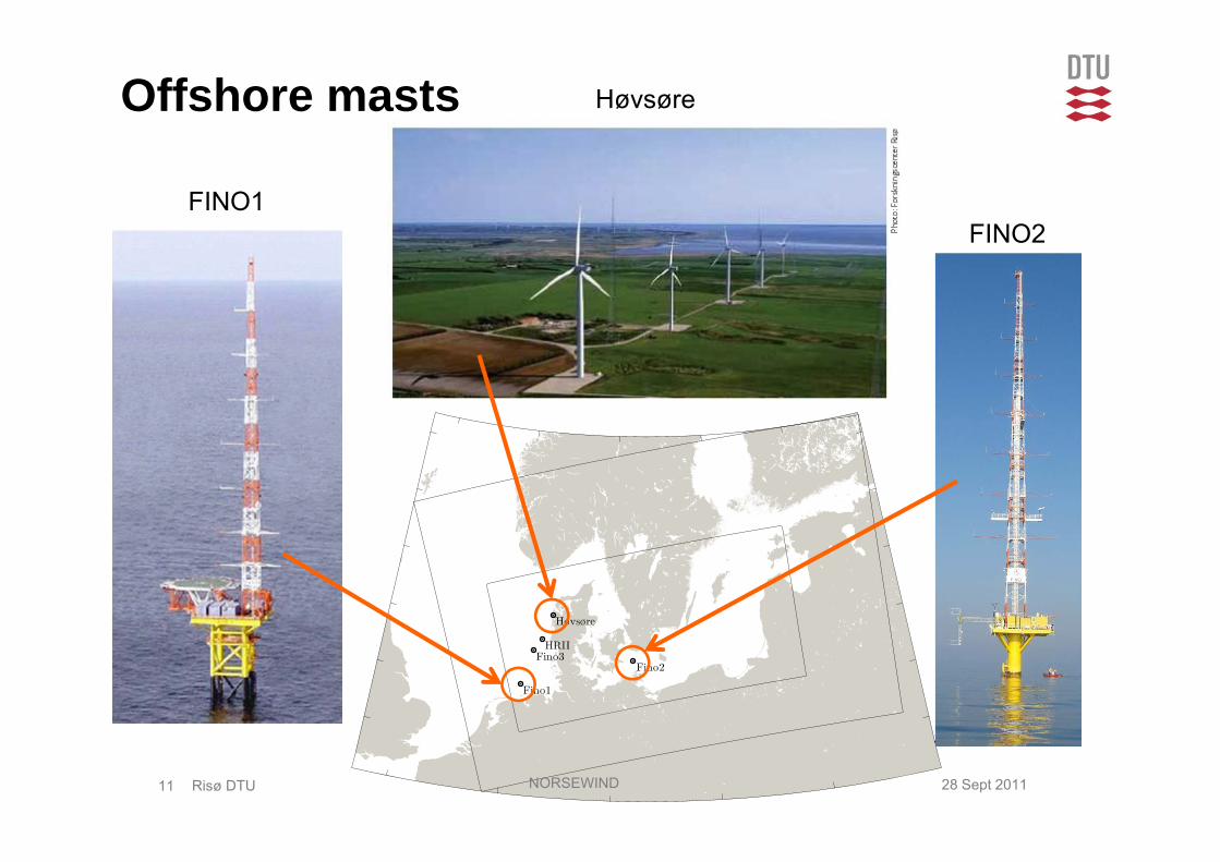
11 Risø DTU 28 Sept 2011 NORSEWIND
Offshore masts
FINO1FINO2
Høvsøre
12 Risø DTU
Validation of downscaling wind profiles, October 2009
6 boundary layer schemesSame model setup
LAND
OCEAN 1/25/2012Andrea Hahmann
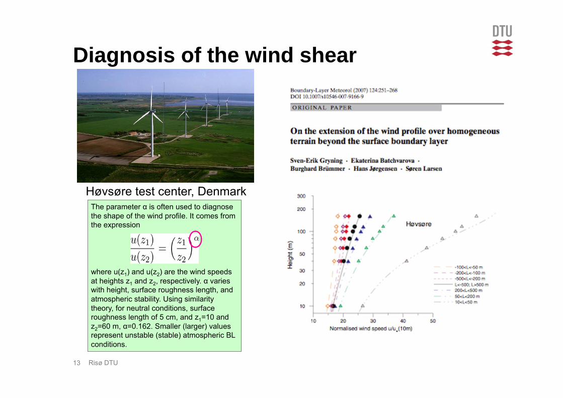
13 Risø DTU
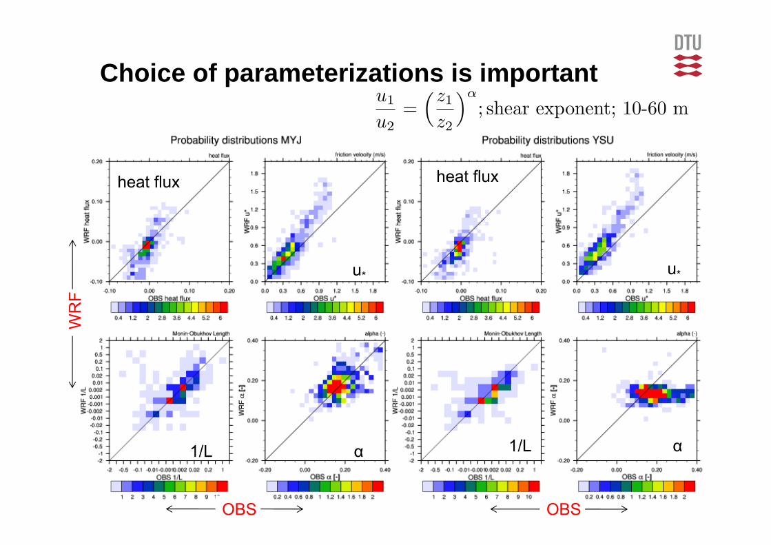
Diagnosis of the wind shear
The parameter α is often used to diagnose the shape of the wind profile. It comes from the expression
where u(z1) and u(z2) are the wind speeds at heights z1 and z2, respectively. α varies with height, surface roughness length, and atmospheric stability. Using similarity theory, for neutral conditions, surface roughness length of 5 cm, and z1=10 and z2=60 m, α=0.162. Smaller (larger) values represent unstable (stable) atmospheric BL conditions.
Høvsøre test center, Denmark
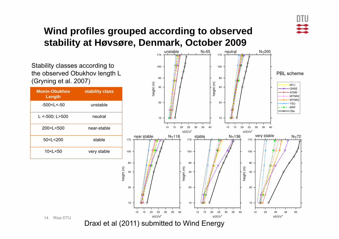
14 Risø DTU
Monin-ObukhovLength
stability class
-500<L<-50 unstable
L <-500; L>500 neutral
200<L<500 near-stable
50<L<200 stable
10<L<50 very stable
Stability classes according to the observed Obukhov length L (Gryning et al. 2007)
Wind profiles grouped according to observed stability at Høvsøre, Denmark, October 2009
PBL scheme
Draxl et al (2011) submitted to Wind Energy
15 Risø DTU
Choice of parameterizations is important
heat flux
u*
1/L α
heat flux
u*
1/L α
WR
F
OBS OBS
16 Risø DTU
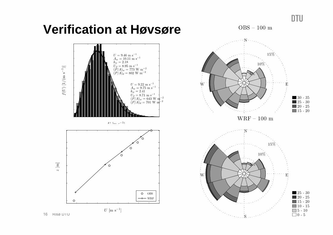
Verification at Høvsøre

17 Risø DTU
Verification(30-100 meters)
Based on these (and other) statistics – choose MYJ PBL scheme
1/25/2012Andrea Hahmann
18 Risø DTU
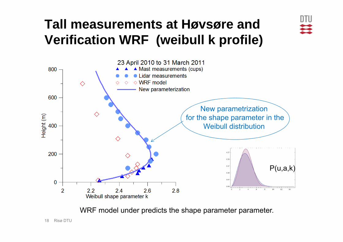
WRF model under predicts the shape parameter parameter.
New parametrizationfor the shape parameter in the
Weibull distribution
Tall measurements at Høvsøre and Verification WRF (weibull k profile)
P(u,a,k)
19 Risø DTU
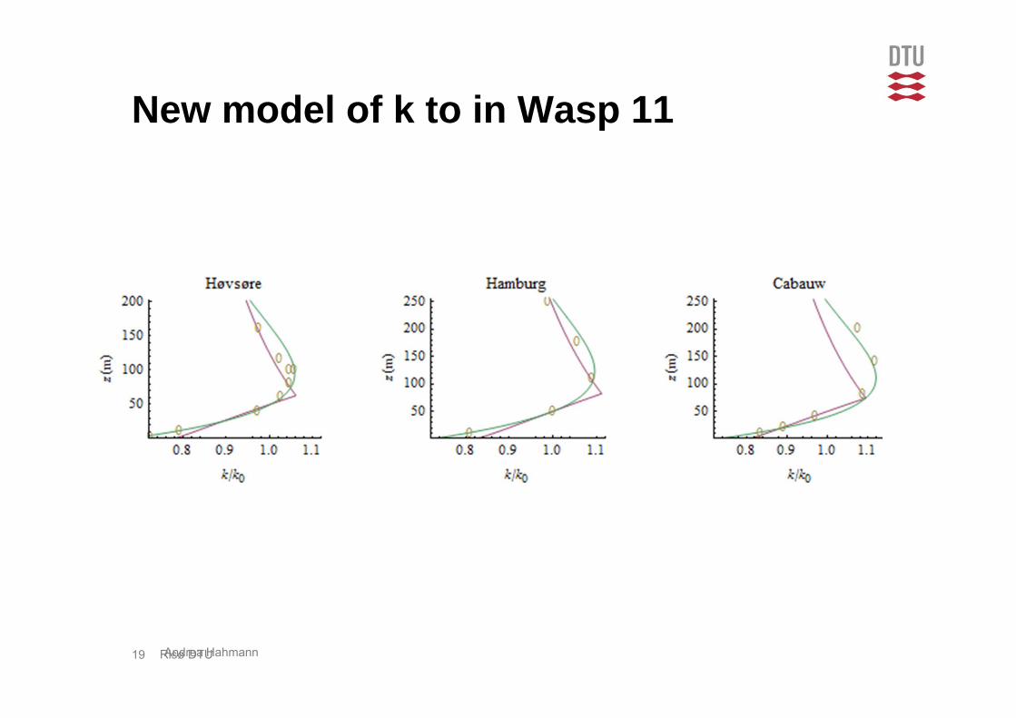
New model of k to in Wasp 11
Andrea Hahmann
20 Risø DTU
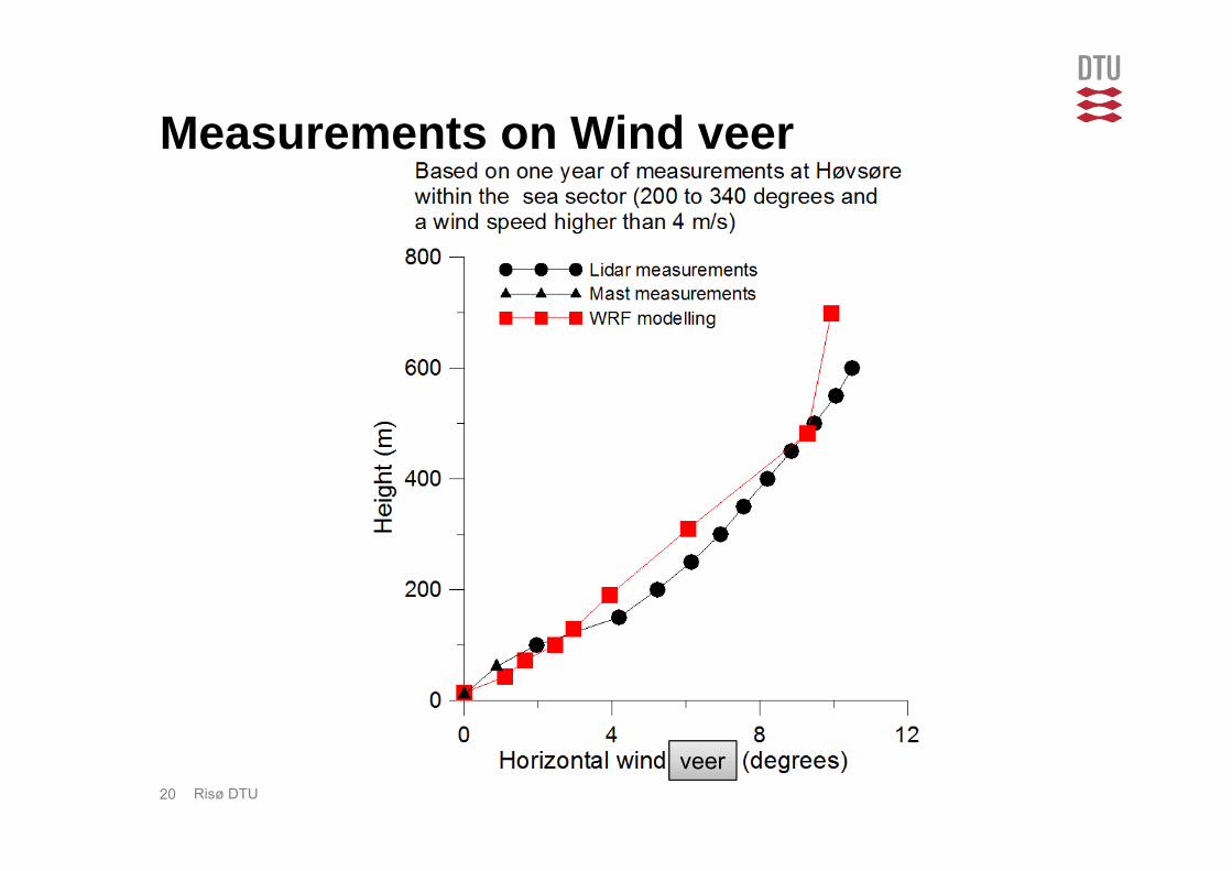
Measurements on Wind veer
veer
21 Risø DTU
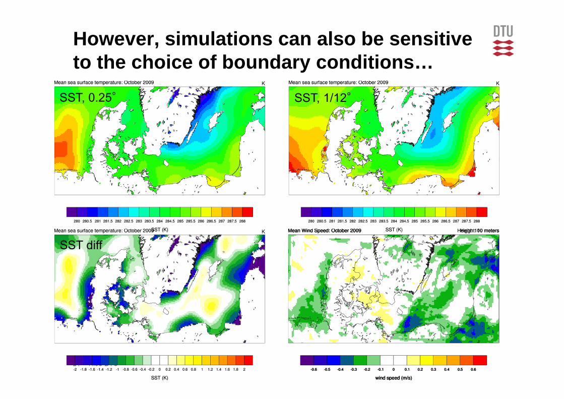
However, simulations can also be sensitive to the choice of boundary conditions…
SST, 0.25° SST, 1/12°
SST diff U 10m diff

22 Risø DTU
Determination of long-term stability by mesoscale model data
• For most applications, estimates of wind and wind shear at 100 m are required. At this level the effect of atmospheric stability is important
• Most offshore measurement sites (e.g., Lidar) do not have means to estimate stability
• Long-term stability is required for:– input to micro-scale models (e.g.
WAsP)
– “Lift” satellite-derived wind measurements (QuikSCAT, SAR) to hub height
• It could be possible to use mesoscale models output (like WRF) to derive stability
1/25/2012Andrea Hahmann
Theoretical formulation of the distribution of atmospheric stability (1/L)
at Horns Rev M2
bulkmeasurements
WRF
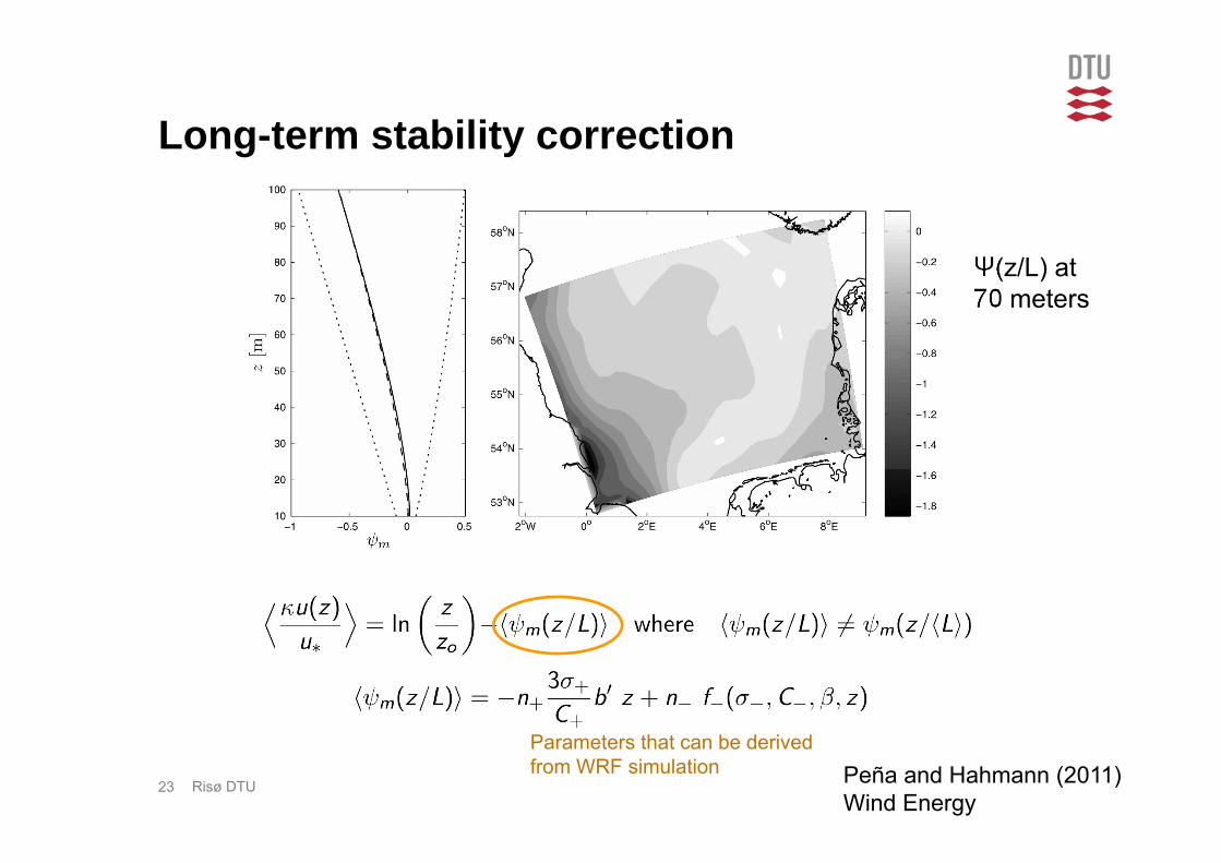
23 Risø DTU
Ψ(z/L) at 70 meters
Long-term stability correction
Peña and Hahmann (2011)Wind Energy
Parameters that can be derivedfrom WRF simulation
INTERNATIONAL JOURNAL OF CLIMATOLOGYInt. J. Climatol. 31: 1584–1595 (2011)Published online 2 June 2010 in Wiley Online Library(wileyonlinelibrary.com) DOI: 10.1002/joc.2175
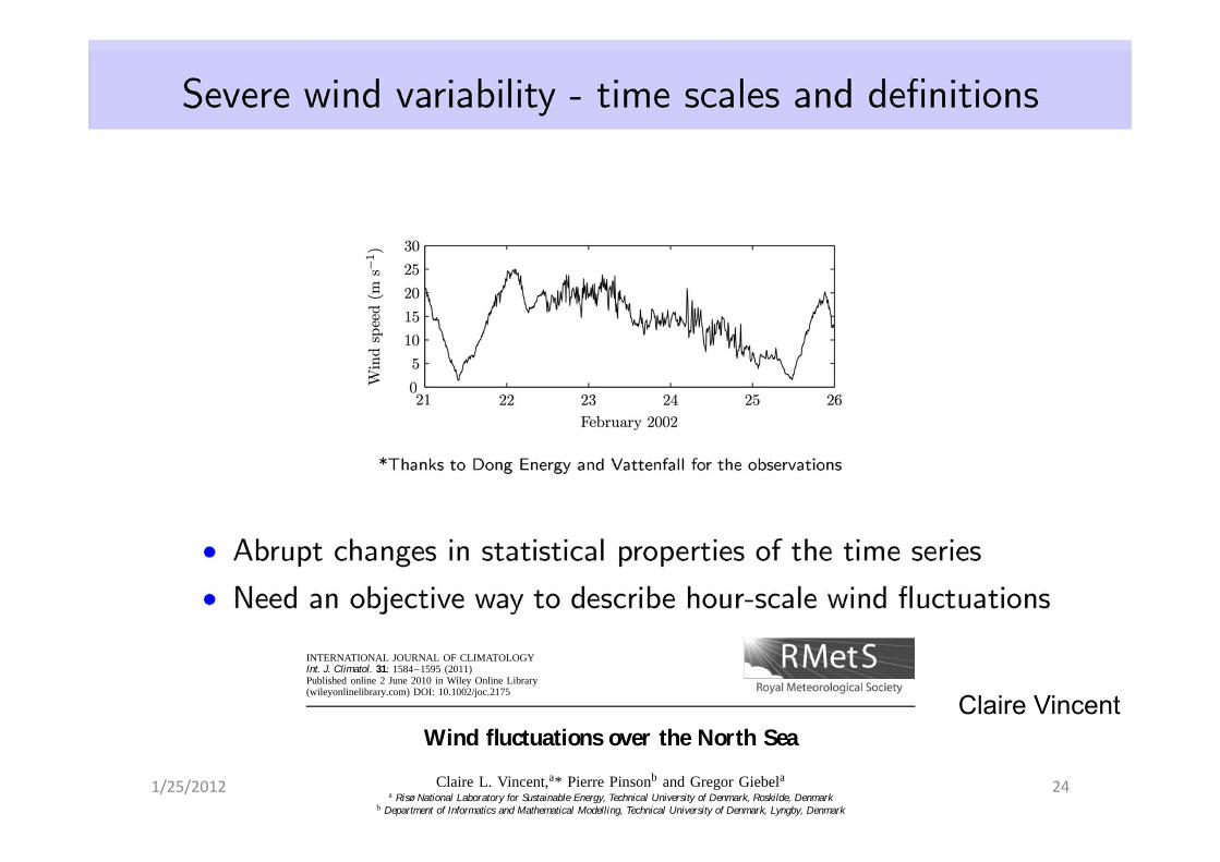
Wind fluctuations over the North Sea
Claire L. Vincent,a* Pierre Pinsonb and Gregor Giebelaa Risø National Laboratory for Sustainable Energy, Technical University of Denmark, Roskilde, Denmark
b Department of Informatics and Mathematical Modelling, Technical University of Denmark, Lyngby, Denmark
Claire Vincent
1/25/2012 24
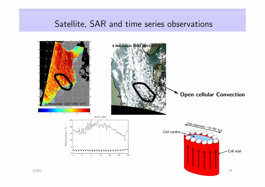
1/25/2012 Andrea Hahmann 25
1/25/2012 Andrea Hahmann 26
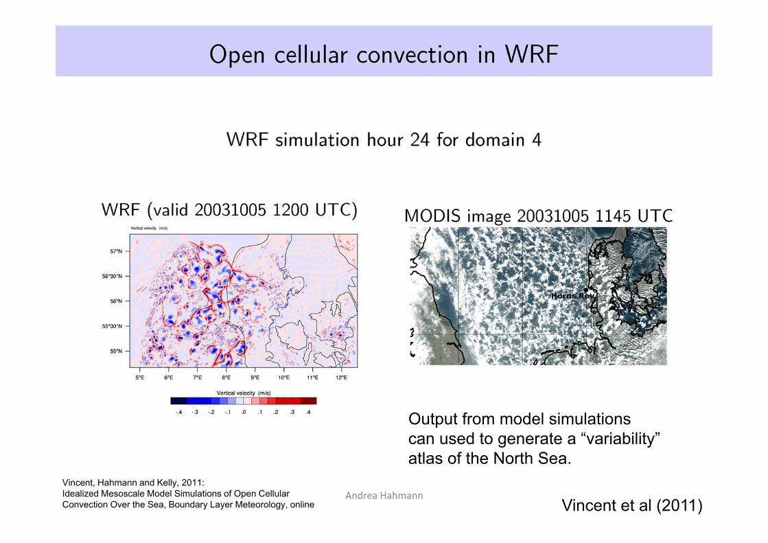
Output from model simulationscan used to generate a “variability”atlas of the North Sea.
Vincent et al (2011)Vincent, Hahmann and Kelly, 2011: Idealized Mesoscale Model Simulations of Open Cellular Convection Over the Sea, Boundary Layer Meteorology, online
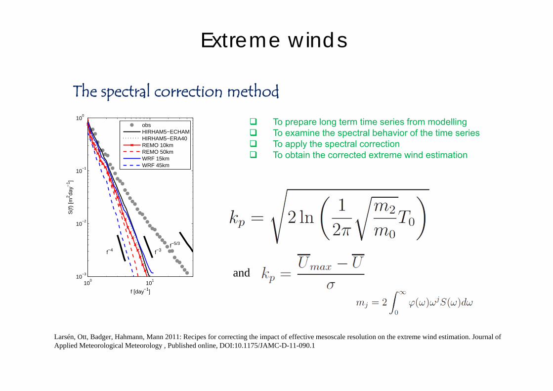
Extreme winds
The spectral correction method
100
101
10−3
10−2
10−1
100
f [day−1]
S(f
) [m
2 day−
1 ]
f−5/3
f−3f−4
obsHIRHAM5−ECHAMHIRHAM5−ERA40REMO 10kmREMO 50kmWRF 15kmWRF 45km
To prepare long term time series from modelling To examine the spectral behavior of the time series To apply the spectral correction To obtain the corrected extreme wind estimation
Larsén, Ott, Badger, Hahmann, Mann 2011: Recipes for correcting the impact of effective mesoscale resolution on the extreme wind estimation. Journal of Applied Meteorological Meteorology , Published online, DOI:10.1175/JAMC-D-11-090.1
and
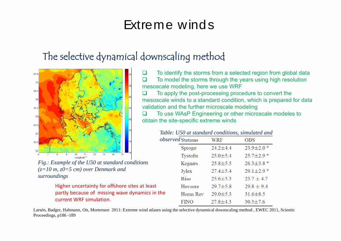
Extreme winds
To identify the storms from a selected region from global data To model the storms through the years using high resolution mesoscale modeling, here we use WRF To apply the post-processing procedure to convert the mesoscale winds to a standard condition, which is prepared for data validation and the further microscale modeling To use WAsP Engineering or other microscale modeles to obtain the site-specific extreme winds
Higher uncertainty for offshore sites at leastpartly because of missing wave dynamics in the current WRF simulation.
The selective dynamical downscaling method
Table: U50 at standard conditions, simulated and observed
Fig.: Example of the U50 at standard conditions(z=10 m, z0=5 cm) over Denmark and surroundings
Larsén, Badger, Hahmann, Ott, Mortensen 2011: Extreme wind atlases using the selective dynamical downscaling method , EWEC 2011, ScienticProceedings, p186 -189

25/01/2012Review 429 Risø DTU, Technical University of Denmark
– Main features of FUGA a Lin. Wake model
• Solves linearized RANS equations• Closure: mixing length, k- or ’simple’ (t=u*z) • Fast, mixed-spectral solver using pre-calculated look-up tables (LUTs)• No computational grid, no numerical diffusion, no spurious mean
pressure gradients• Integration with WAsP: import of wind climate and turbine data. • 106 times faster than conventional CFD!
GUI
Validation

25/01/2012Review 430 Risø DTU, Technical University of Denmark
Meandering of Wakes and the application to wake defecit
• In DWM meandering is modelled as if the wake was a passive scalar diffusing Mann turbulence. This approach will be tried, but we expect it to seriously slow down computation time.
• As an alternative we will try a simpler model and adjust it to the Mann turbulence model and/or to data (how?). The simple model follows a fluid particle backwards in time and from a rotor to see how many upwind rotors it has passed through. From this the accumulated velocity deficit can be estimated.
• The simple model is based on a Langevin equation. The model has two parameters: a turbulence velocity v and a Lagrangian time scale TL.
• The slowest part of the meandering will only causes a general trend during 10 minutes. This part can be estimated from data...
25/01/2012Review 431 Risø DTU, Technical University of Denmark
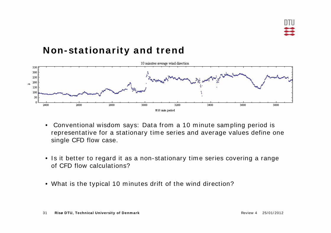
Non-stationarity and trend
• Conventional wisdom says: Data from a 10 minute sampling period is representative for a stationary time series and average values define one single CFD flow case.
• Is it better to regard it as a non-stationary time series covering a range of CFD flow calculations?
• What is the typical 10 minutes drift of the wind direction?

25/01/2012Review 432 Risø DTU, Technical University of Denmark
Drift• Definitions:
Wind direction : 10 minutes average of : a
Drift of a during 10 minutes: a=a(t+10min)-a(t)
Rms value of a : a = <(a)2>½
• a is a measure of the linear drift of the average wind direction during 10 minutes.
• a can be obtained from 10 minutes average wind vane data.
a = 4.7 degrees
Horns Rev 1 met mast data

25/01/2012Review 433 Risø DTU, Technical University of Denmark
Effect of mean value drift (a sort of meandering)
0,40
0,50
0,60
0,70
0,80
0,90
1,00
1,10
1 2 3 4 5 6 7 8
No
rmal
ized
pro
du
ctio
n
Row number
Data
Fuga witout drift
Fuga with drift
Nysted 278O+/-2.5O bin
25/01/2012Review 434 Risø DTU, Technical University of Denmark
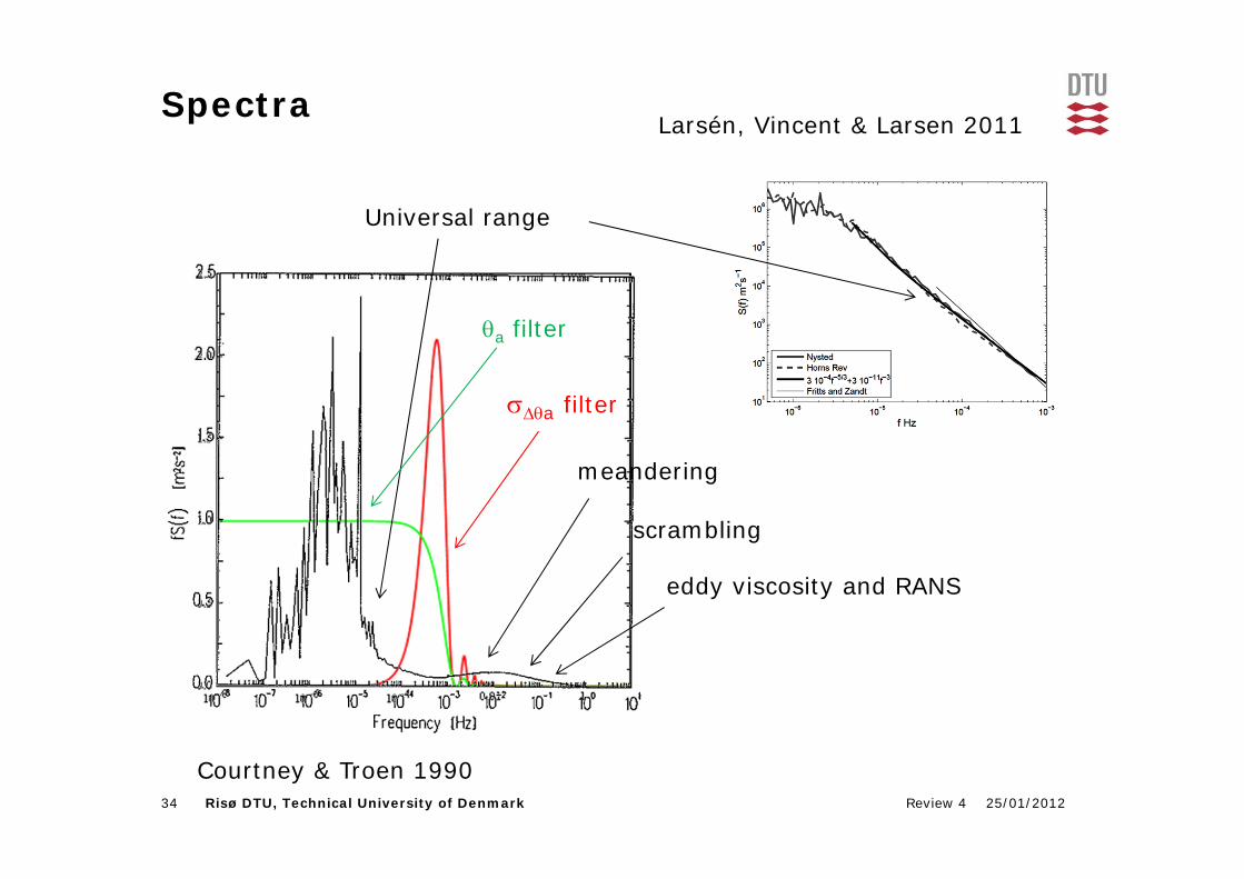
Spectra
Courtney & Troen 1990
Larsén, Vincent & Larsen 2011
a filter
Universal range
a filter
meandering
scrambling
eddy viscosity and RANS

25/01/2012Review 435 Risø DTU, Technical University of Denmark
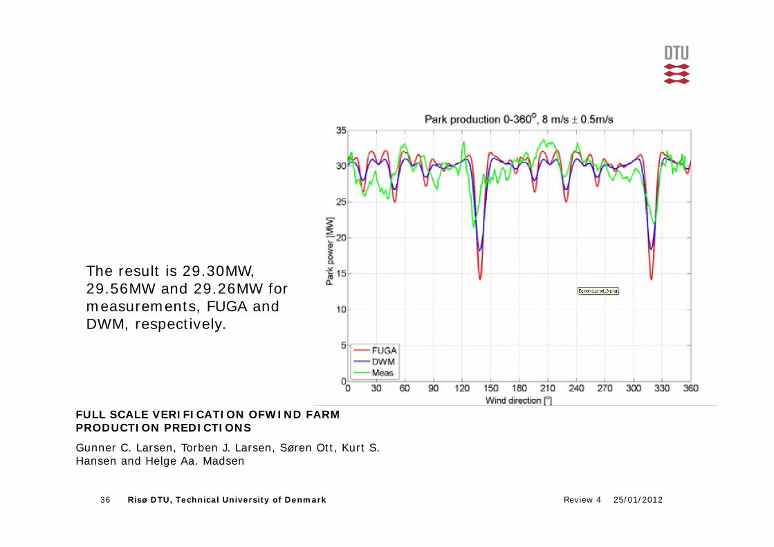
The Egmond aan Zee wind farm
25/01/2012Review 436 Risø DTU, Technical University of Denmark
The result is 29.30MW, 29.56MW and 29.26MW for measurements, FUGA and DWM, respectively.
FULL SCALE VERIFICATION OFWIND FARM PRODUCTION PREDICTIONS
Gunner C. Larsen, Torben J. Larsen, Søren Ott, Kurt S. Hansen and Helge Aa. Madsen
25/01/2012Review 437 Risø DTU, Technical University of Denmark
Summary of applications of mesoscale modelingactivities
Meso-scale modeling offshore have proven to be very use full according the following list:
• Wind power resources and forecasting – power distribution modeling– combination of dynamical and statistical methods– Wind atlas applications (extremes, variability, correlations
etc)– assimilation of wind farm data (nacelle winds and yaw
angles)– Prediction of the meandering characteristic for wake deficit
– used for optimizing windfarm layout• Forecasting icing occurrence and ice amount on turbine blades
in cold climate• External design parameters for wind farm design (extremes,
shear, veer not turbulence -sofar)
1/25/2012 Andrea Hahmann 37
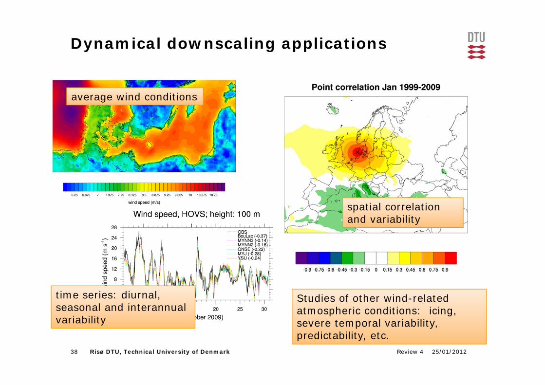
25/01/2012Review 438 Risø DTU, Technical University of Denmark
Dynamical downscaling applications
average wind conditions
spatial correlation and variability
time series: diurnal, seasonal and interannual variability
Studies of other wind-related atmospheric conditions: icing, severe temporal variability, predictability, etc.


![ATP 08 Soeren Schmidt nsls2 rev [Read-Only] · Total: 165.263 99% matched Søren Schmidt, Risø DTU DAQ and user interface workshop, ... Søren Schmidt, Risø DTU DAQ and user interface](https://static.fdocuments.net/doc/165x107/5b384c6c7f8b9abd438d0c61/atp-08-soeren-schmidt-nsls2-rev-read-only-total-165263-99-matched-soren.jpg)