Decomposing Cross-Sectional Vaolatility · set for active portfolio management. For instance, ......

MSCI Research © 2010 MSCI. All rights reserved. 1 of 21 Please refer to the disclaimer at the end of this document.

Decomposing Cross-Sectional Volatility

September 2010

Jose Menchero Andrei Morozov

Decomposing Cross-Sectional Volatility | September 2010

MSCI Research © 2010 MSCI. All rights reserved. 2 of 21 Please refer to the disclaimer at the end of this document. RV0710

Introduction

Cross-sectional volatility (CSV) is defined as the standard deviation of a set of asset returns over a period. This dispersion measure is of fundamental importance, as it represents the opportunity set for active portfolio management. For instance, if the dispersion of stock returns is very small, then all stocks behave similarly and there is little opportunity to outperform the market. Conversely, when CSV levels are high, performance differences among active managers are more pronounced, as shown by Ankrim and Ding (2002).

A useful characteristic of CSV is that, unlike time-series volatility, it uses only the most recent information. In fact, Solnik and Roulet (2000) showed that under a set of simplifying assumptions, cross-sectional data could be used to provide an “instantaneous” measure of realized correlation.

Another question of major interest for global equity portfolio managers is the relative importance of industries versus countries. If country effects dominate, then primary investment consideration should be given to the country allocation decision. On the other hand, if global economic integration is lessening the distinctions between countries, then an industry-first investment process may be more appropriate.

The industry-versus-country question has received much attention over the years. One early study was by Grinold, Rudd, and Stefek (1989), who used a global multi-factor model to show that countries had greater explanatory power than industries over the period 1983-1988. Heston and Rouwenhorst (1995) also studied the issue; they constructed a factor model for developed Europe containing 7 industries and 12 countries and found that country factors were far more volatile than their industry counterparts over the period 1978-1992. However, in a subsequent study, Cavaglia, Brightman, and Aked (2000) investigated a broader universe comprising 21 developed markets and 36 industries and found that industry effects had overtaken country effects in the late 1990s.

More recently, Puchkov, Stefek, and Davis (2005) used a two-tiered factor model to study the relative importance of countries, global industries, global styles, and purely local factors. They found that countries nearly always dominated global industries in developed markets over the period 1992-2004. The exception is the sub-period from 1999-2002, when the two effects were comparable. In their approach, global styles were found to be far weaker than either countries or global industries.

While the above studies certainly helped shed light on the drivers of global equity returns, they share one or more basic shortcomings. First, style factors are either entirely missing or estimated in a manner that masks their full strength. For instance, style factors are completely absent from the models used by Heston and Rouwenhorst (1995), as well as Cavaglia, Brightman, and Aked (2000). In the model used by Grinold, Rudd, and Stefek (1989), the effect of market beta is combined with the country factor rather than attributed to a style factor. Naturally, this makes country effects seem stronger at the expense of style factors. The second basic shortcoming is that some of the models do not treat industries and countries symmetrically. For instance, the inclusion of market beta with the country factor by Grinold, Rudd, and Stefek (1989) gives a



material advantage to country factors over industries. Similarly, the estimation methodology employed Puchkov, Stefek, and Davis (2005) gives preferential treatment to country factors at the expense of industries and styles, as we later discuss.

In this paper, we present a new framework for analyzing cross-sectional volatility and investigating the relative importance of countries, industries, and styles. Our methodology provides an exact decomposition of CSV into contributions from individual factors. These contributions can then be cleanly aggregated to answer questions regarding the net strength of entire categories of factors. Furthermore, our approach treats all factors (i.e., countries, industries, and styles) on an equal footing, and thus represents a powerful new tool for investigating the relative importance of these drivers of global equity returns.

Time-Series x-sigma-rho Attribution

Before presenting our decomposition of cross-sectional volatility, it is useful to briefly discuss attribution of time-series volatility. In general, a portfolio’s return tR over period t can be attributed to a set of sourcesm ,

t m mt

m

R x g, (1)

where mx is the portfolio exposure to the source and mtg is the return of the source. As shown by Menchero and Davis (2010), the time-series volatility of the portfolio R can be attributed to the same sources via the x-sigma-rho formula:

,m m m

m

R x g g R . (2)

Here, mg is the time-series volatility of source m , and ,mg R is the time-series correlation between source m and the portfolio return. This intuitive formula states that there are three drivers of portfolio volatility: (a) the size of the position, x, (b) the stand-alone volatility of the source, sigma, and (c) the correlation between the source and the overall portfolio, rho. This risk attribution framework has also been generalized to the case of extreme risk, as discussed by Goldberg, Hayes, Menchero, and Mitra (2010).

Cross-Sectional x-sigma-rho Attribution

The x-sigma-rho formula can be further extended to decompose cross-sectional volatility. Suppose that the return of stock n is expressed according to a multi-factor model,

n k nk n

k

r f X u , (3)



where kf is the return of factor k , nkX is the stock exposure to the factor, and nu is the idiosyncratic return not explained by the factors. The CSV is defined as

2

n nnr w r r

, (4)

where nw is the weight of stock n , and r is the mean return of the estimation universe. As shown in Appendix A, application of the x-sigma-rho formula yields

, ,k k k

k

r f X X r u u r . (5)

This states that there are three drivers of CSV due to factors: (a) the magnitude of the factor return, kf (b) the cross-sectional volatility of the factor exposures, kX and (c) the cross-sectional correlation between the factor exposure and the stock returns, ,kX r . Note that in going from the time-series view to the cross-sectional perspective, the roles of factor exposures and factor returns are effectively interchanged.

Equation 5 also states that there are two drivers of CSV arising from the idiosyncratic component. The first is the CSV of the specific returns, u ; the second driver is the cross-sectional correlation ,u r between the specific returns and the stock returns.

Global Factor Model

To investigate the relative importance of countries, industries, and styles, we construct a global factor model that contains a world factor, 48 country factors spanning both developed markets and emerging markets, 24 industry groups based on the Global Industry Classification Standard (GICS®), and 8 style factors. The model is derived from the Barra Global Equity Model, GEM2, as described by Menchero, Morozov, and Shepard (2010), but with several notable modifications as we now discuss.

First, to avoid introducing biases in favor of either country or industry factors, we standardize all style factors on a global-relative basis. By contrast, for purposes of maximizing the explanatory power of the model, GEM2 standardizes some style factors on a global-relative basis and others on a country-relative basis. Second, we use 24 industry groups for our study, versus 34 industry factors used in GEM2. For present purposes, we adhere to a single level of the GICS hierarchy with slightly fewer industries than countries. By contrast, the 34 GEM2 industry factors were designed to maximize the explanatory power of the model within a relatively parsimonious factor structure. Obviously, if the GEM2 industry factors were used, it would give added importance to the industry factors, although it would not alter the main conclusions of this paper. Finally, we use full market-capitalization regression weighting, versus square-root market-cap weighting in GEM2. Whereas square-root weighting is more appropriate for risk forecasting purposes, full cap weighting is more relevant for active managers seeking investment opportunities.



The stock returns within our global factor model are given by

( ) ( )n w c n i n ns s n

s

r f f f X f u . (6)

Here, wf is the return of the world factor, ( )c nf and ( )i nf are the country and industry factor returns pertaining to stock n , nsX is the stock exposure to style factor s , sf is the return of the style factor, and nu is the specific return of the stock.

The eight style factors are taken from the Barra GEM2 model and are described in detail by Menchero, Morozov, and Shepard (2010). The style factors include volatility, momentum, size, value, growth, leverage, liquidity, and non-linear size. Note that the volatility factor essentially captures the effect of market beta. Style factors are standardized to have a cap-weighted mean of zero and standard deviation equal to one over the estimation universe. The estimation universe is taken as the MSCI All Country World Investable Market Index (ACWI IMI), a broad index that aims to reflect the full breadth of investment opportunities in developed and emerging markets.

We perform monthly cross-sectional regressions from January 1993 through April 2010. Note that the regression in Equation 6 contains two exact collinearities. Namely, the sum of country factor exposures replicates the world factor exposure, and likewise for the sum of industry factors. Therefore, two constraints must be applied to obtain a unique solution. We follow the approach of Heston and Rouwenhorst (1995) and set the sum of cap-weighted country and industry factor returns to zero every period.

Under this model specification, the pure world factor portfolio is represented by the cap-weighted estimation universe. The pure country factor portfolios are 100 percent long the particular country, 100 percent short the world portfolio, and have zero exposure to every industry and style factor. Similarly, pure industry factor portfolios are 100 percent long the particular industry, 100 percent short the world portfolio, and have zero exposure to every country and style factor. Finally, pure style factors have unit exposure to the particular style, and zero exposure to every other style factor, country, and industry. This regression approach cleanly disentangles the effects of multi-collinearity, and captures the pure effect for every factor. For a more in-depth discussion of factor portfolios, see Menchero (2010).

Empirical Results

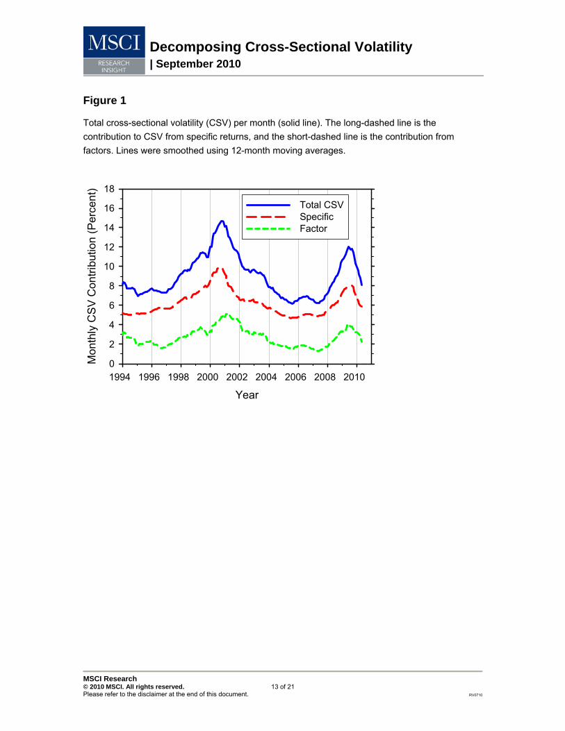
In Figure 1, we report the total CSV from January 1994 to April 2010, as well as the contributions from factors and stock-specific sources. Results were computed using cap weights, and lines were smoothed using 12-month rolling averages. Note that average CSV levels vary widely, ranging from a peak of 14 percent monthly in the wake of the internet bubble to a low of under 7 percent during the 2005-2007 bull market.



Over the sample period, most of the CSV was explained by the idiosyncratic component, reflecting the high “noise” levels characteristic of equity returns. The ratio of the factor CSV contribution to the total CSV gives the relative 2R of the model,

22

21n n

R

n n

w uR

w r r

, (7)

where r is the mean return of the estimation universe. For instance, from Figure 1 we see that in January 1994 the explained CSV was about 3 percent versus a total CSV of roughly 8 percent. The relative 2R , therefore, was approximately 38 percent.

In Figure 2, we examine the contribution to CSV by factor type. In the mid-1990s, countries strongly dominated industries. Beginning in 1999, however, industries overtook countries in importance, consistent with the findings of Cavaglia, Brightman, and Aked (2000). Industries continued to dominate countries for several years, lasting until 2003. From 2003-2007, industries and countries were of comparable strength. Since 2007, however, countries have once again mostly dominated industries, with the gap becoming especially pronounced in 2010.

Perhaps the most striking feature from Figure 2 is the contribution of style factors to CSV. The magnitude varies dramatically, ranging from lows of about 20 bps in 1995 and 2007 to a peak of 270 bps in 2001. In fact, from 2000-2004, styles were the main contributor to CSV, dominating both countries and industries. By contrast, from 2004-2007, styles were the weakest contributor, although they reasserted themselves as the financial crisis unfolded in 2008 and 2009.

A commonly held – but erroneous – view is that style factors are typically less important than either industries or countries. The basis for this misperception is the empirical observation that style factors are typically less volatile than country or industry factors. To understand why style effects can be so strong despite their low volatility, consider the following. Assuming collinearity among the factors to be negligible, Equation 5 can be simplified to give

2 2 21

k kk

r f X ur

. (8)

This approximation says that the contribution to CSV from an individual factor is proportional to the product of the squared factor return and the cross-sectional variance of factor exposures. Although style factors typically have small factor returns compared to countries or industries, their cross-sectional variance is much larger.

More specifically, if kW is the weight of assets with exposure to country or industry k , then the cross-sectional variance of factor exposures is given by

2 2

k k kX W W . (9)

A fairly large country or industry may have a weight of 10 percent, which leads to a cross-sectional variance of 0.09. A typical country, however, may have a weight of only two percent,



which leads to a cross-sectional variance of only about 0.02. By contrast, style factors have cross-sectional variance equal to 1.0 by construction, which is more than 10 times that of a large country/industry and perhaps 50 times that of a typical one. Therefore, although style factor returns may be smaller, this may be more than compensated for by their large cross-sectional variance.

The empirical results in Figure 2 (i.e., that style factors sometimes dominate countries and industries) are in contrast to the earlier work of Puchkov, Stefek, and Davis (2005), who found that global styles were always weaker than countries or industries. We believe that the main source of this discrepancy is that our methodology estimates factor returns directly in a one-step regression that treats all factors on an equal basis, whereas the Puchkov approach uses an indirect, two-step procedure that effectively transfers explanatory power to country factors. More specifically, in the Puchkov approach, local factor returns for industries and styles are first computed within each country. In the second step, these local factor returns are used to estimate global factor returns for countries, industries, and styles. An effect of this estimation procedure is to mask the strength of the style factors. That is, since the style factors are estimated within each country, they will not explain that portion of a country’s return due to a style tilt, which is instead picked up by the country factor.

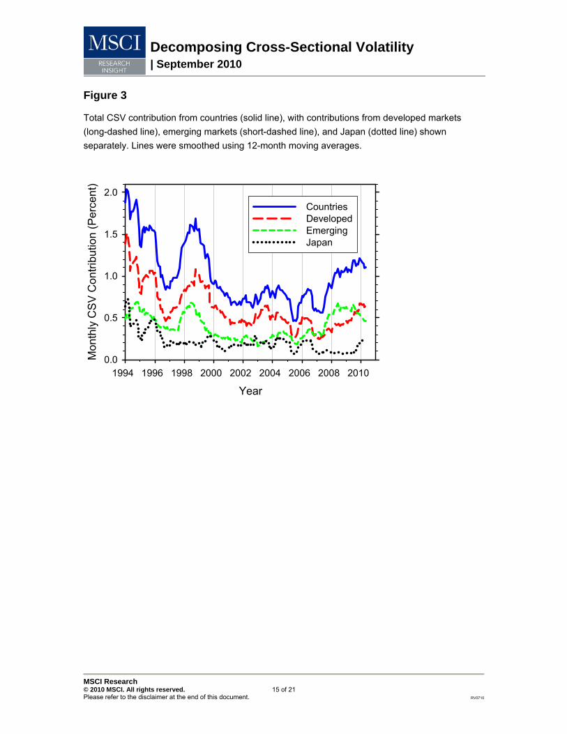
Another question of major interest for international investors is the relative importance of developed markets versus emerging markets. This question can be investigated using our framework by aggregating CSV contributions within each group of factors. In Figure 3, we plot the total CSV contribution from countries and also the contributions from developed markets and emerging markets. In the 1990s, it is clear that developed markets consistently dominated emerging markets. Since 2005, however, emerging markets increased in importance to be roughly on par with developed markets. In fact, during the financial crisis of 2008, emerging markets dominated developed markets by a sizeable gap.

We can also drill into each category of factors. To illustrate this point, in Figure 3 we plot the CSV contribution from Japan, a particularly strong developed-market factor. In the early history, Japan contributed nearly half of the CSV attributed to developed-market factors. Since 1997, this proportion has decreased, although Japan has remained a major contributor to CSV.

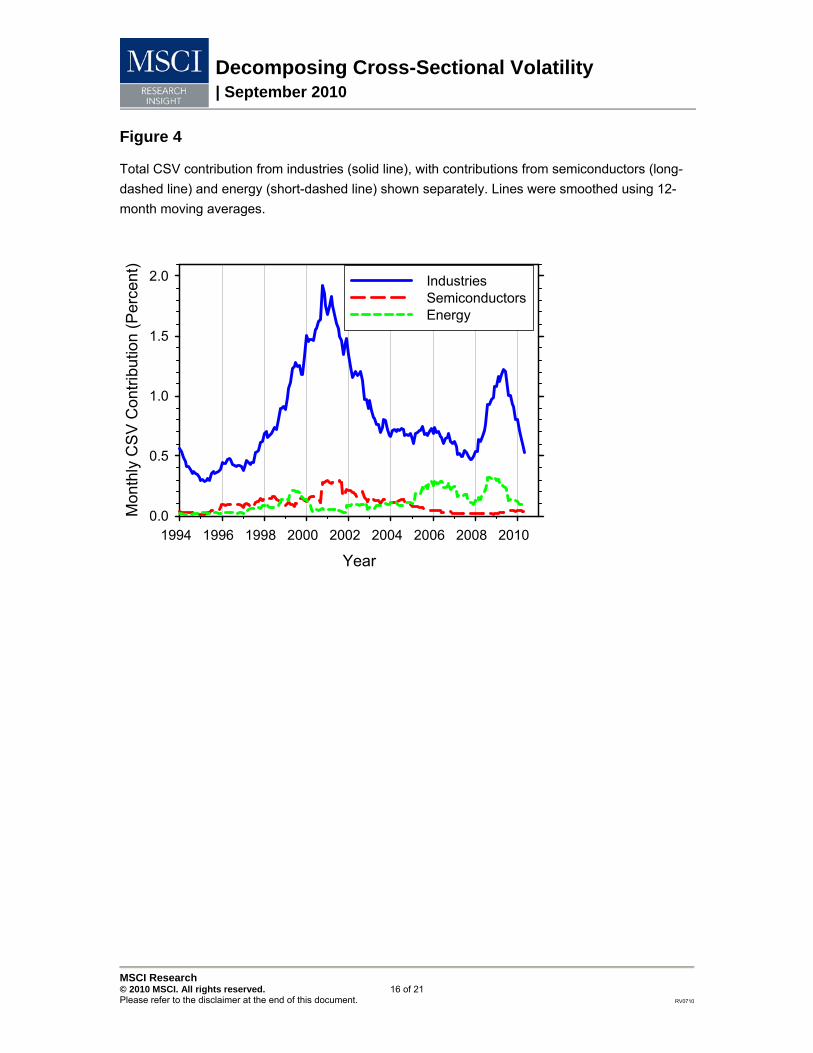
In Figure 4 we plot the total CSV contributions from industries, as well as the individual contributions from the semiconductor and energy industries. Figure 4 clearly illustrates the buildup in strength of the semiconductor factor in the late 1990s. In the wake of the internet bubble, the strength of the semiconductor factor reaches a peak of nearly 30 bps, but has since become considerably weaker. By contrast, the energy factor overtook semiconductors in 2005 and has strongly dominated ever since. In recent years, energy has been one of the main drivers of CSV due to industries.

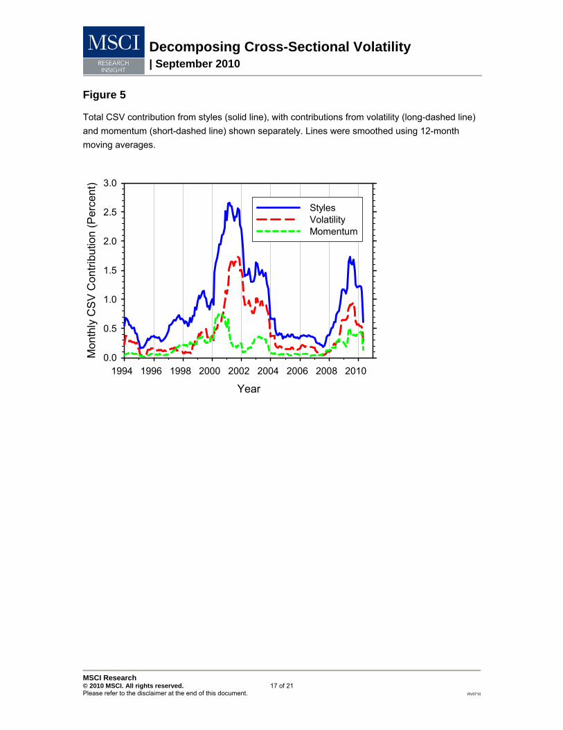
In Figure 5, we present the total CSV contribution from style factors, as well as the individual contributions from the volatility and momentum factors. For most periods – but especially during market turbulence – the volatility factor was the main contributor to styles CSV. There were only a



few, brief periods when momentum was stronger than the volatility factor, and these tended to be periods of relative calm.

An attractive feature of our methodology is that it enables a direct apples-to-apples comparison of the strength of individual country, industry, and style factors. For instance, as seen in Figure 5, the volatility factor made a maximum CSV contribution of about 170 bps, while momentum made a peak contribution of roughly 70 bps. By contrast, even a strong industry factor such as energy rarely exceeded 30 bps. Japan, a particularly strong country factor, made a maximum CSV contribution of about 70 bps, but has contributed in the range of 10-30 bps since 1997.

Traditional managers are primarily interested in performance relative to a benchmark, and hence CSV is of the greatest relevance. Hedge fund managers, on the other hand, may be more interested in the drivers of absolute returns. To identify the drivers of absolute returns, we use the root mean squared (RMS) return, defined as

2

n nns r w r

. (10)

Note that since the RMS measure uses absolute returns (as opposed to relative returns), it is strictly larger than CSV. In Appendix A, we show how to apply the x-sigma-rho formula to decompose RMS into contributions from individual factors.

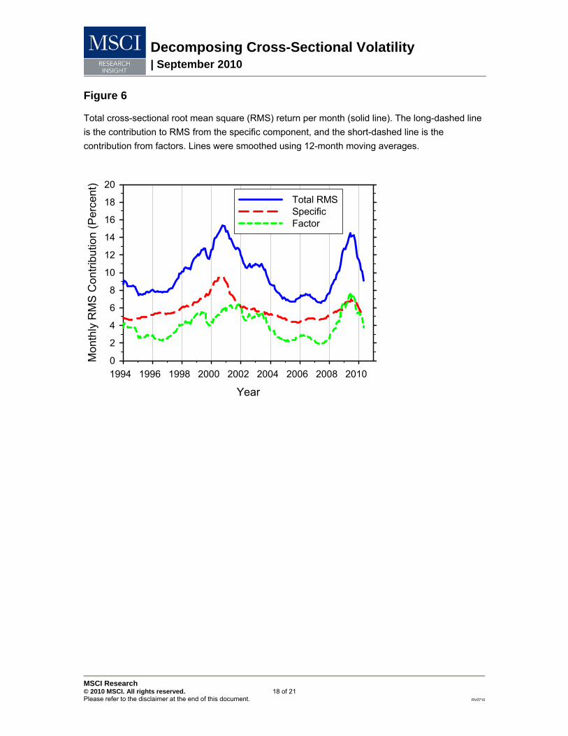
In Figure 6 we plot total RMS levels, as well as contributions from factors and stock-specific sources. The total RMS is qualitatively similar to the total CSV presented in Figure 1, except that total RMS levels are slightly higher than CSV levels, as expected. A more significant difference is that the factor contribution to RMS is significantly greater than the factor contribution to CSV. The underlying reason is that the world factor contributes to RMS, but not to CSV. This can be seen mathematically from Equation 5, since the CSV of the world factor is zero. By contrast, the RMS of the world factor is 1, which contributes to total RMS via Equation A17. In essence, the world factor explains the mean return of the estimation universe, but cannot explain anything relative to

the mean.

The total 2R of the model is defined as

22

21

n nT

n n

w uR

w r

. (11)

The ratio of the factor contribution to RMS to the total RMS gives the total 2R of the model. During periods of extreme market volatility, such as 2009, the factors actually contributed more to RMS than the specific returns, indicating that the total 2R of the model exceeded 50 percent during these periods.

In Figure 7, we plot the contribution to RMS return coming from countries, industries, styles, and the world factor. Comparing Figure 7 to Figure 2, we identify many similarities. For instance, countries dominated industries from 1994-1999, and industries surpassed countries from 1999-2003. Moreover, styles dominated both countries and industries from 2000-2004 in both figures.



The distinctive feature of Figure 7 is that it shows the contribution of the world factor. On average, the world factor was on par with the other factor categories in explaining RMS. During times of extreme market turbulence, however, the world factor easily dominated the other sources of absolute returns. For instance, during the height of the financial crisis in 2009, the world factor dwarfed the other factor categories in terms of explaining RMS returns.

Summary

We present a new framework for analyzing the global equity markets. Our approach leverages the x-sigma-rho attribution methodology to provide a decomposition of cross-sectional volatility. This enables us to identify the drivers of CSV at the individual factor level, or to aggregate contributions to find the relative importance of each factor category. We use our approach to investigate the relative importance of industries, countries, and styles, as well as to study the strength of emerging markets versus developed markets. The methodology can also be extended to decompose RMS returns, which are more relevant for absolute return managers.



Appendix A

Suppose that stock returns nr are driven by K factors and an idiosyncratic term nu ,

1

K

n k nk nk

r f X u

, (A1)

where nkX is the exposure of stock n to factor k , and kf is the factor return. For notational efficiency, it is convenient to incorporate the idiosyncratic term into the factor component,

1

1

K

n k nkk

r f X

, (A2)

where the idiosyncratic “factor return” is 1 1Kf , and the “factor exposure” is , 1n K nX u . The cross-sectional variance of stock returns is given by

22

n nn

r w r r , (A3)

where nw is the weight of stock n used for the variance computation. Any weighting scheme is permissible, subject to the usual condition that the weights are positive and add to unity. The mean stock return is defined as

n n

n

r w r, (A4)

which can be expressed as

1

1

K

k kk

r f X

, (A5)

where

k n nk

n

X w X. (A6)

Therefore, the excess stock return can be expressed as

1

1

K

n k nk kk

r r f X X

. (A7)

The cross-sectional variance in Equation A3 can therefore be rewritten as

12

1

K

n n k nk kn k

r w r r f X X

, (A8)

which can be rearranged to give

12

1

K

k n nk k nk n

r f w X X r r

. (A9)



The cross-sectional variance of source exposures is given by

22

k n nk kn

X w X X , (A10)

and the cross-sectional correlation between source exposures and stock returns is

,n nk k nn

kk

w X X r rX r

X r

. (A11)

Substituting Equation A11 into Equation A9 provides the decomposition of cross-sectional volatility into its component sources

1

1

,K

k k kk

r f X X r

. (A12)

If we wish to separate the idiosyncratic term, we obtain

1

, ,K

k k kk

r f X X r u u r

, (A13)

which is Equation 5 of the main text. Equation A13 represents an exact decomposition of cross-sectional volatility.

In some instances, it is of interest to decompose not the cross-sectional volatility, but rather the cross-sectional root mean squared (RMS) return s r , defined by

2 2

n nn

s r w r. (A14)

Similarly, the RMS for individual factors is given by

2 2

k n nkn

s X w X. (A15)

We can also define the “pseudo correlation”

,n nk nn

kk

w X rX r

s X s r

. (A16)

Like a standard correlation, the pseudo correlation is bounded between 1 . The only difference between ,kX r and the standard correlation given by Equation A11 is that the latter uses demeaned variables, whereas the former does not. The cross-sectional RMS return can be decomposed as

1

, ,K

k k kk

s r f s X X r s u u r

, (A17)

which is the RMS counterpart of Equation A13.



References

Ankrim, Ernest M., and Zhuanxin Ding. 2002. “Cross-Sectional Volatility and Return Dispersion.” Financial Analysts Journal, vol. 58, no. 5 (September/October): 67-73.

Cavaglia, Stefano, Christopher Brightman, and Michael Aked. 2000. “The Increasing Importance of Industry Factors.” Financial Analysts Journal, vol. 56, no. 5 (September/October): 41-54.

Goldberg, Lisa, Michael Hayes, Jose Menchero, and Indrajit Mitra. 2010. “Extreme Risk Analysis.” Journal of Performance Measurement, vol. 14, no. 3 (Spring): 17-30.

Grinold, Richard, Andrew Rudd, and Dan Stefek. 1989. “Global Factors: Fact or Fiction?” Journal

of Portfolio Management, vol. 16, no. 1 (Fall): 79-89.

Heston, Steven L., and K. Geert Rouwenhorst. 1995. “Industry and Country Effects in International Stock Returns.” Journal of Portfolio Management, vol. 21, no. 3 (Spring): 53-58.

Menchero, Jose. 2010. “Characteristics of Factor Portfolios.” Working paper.

Menchero, Jose, Andrei Morozov, and Peter Shepard. 2010. “Global Equity Risk Modeling.” In J. Guerard, ed., The Handbook of Portfolio Construction: Contemporary Applications of Markowitz

Techniques. New York, NY: Springer.

Menchero, Jose, and Ben Davis. 2010. “Risk Contribution is Exposure times Volatility times Correlation.” Journal of Portfolio Management, to appear.

Puchkov, Anton V., Dan Stefek, and Mark Davis. 2005. “Sources of Return in Global Investing.” Journal of Portfolio Management, vol. 31, no. 2 (Winter): 12-21.

Solnik, Bruno, and Jacques Roulet. 2000. “Dispersion as Cross-Sectional Correlation.” Financial

Analysts Journal, vol. 56, no. 1 (January/February): 54-61.



Figure 1

Total cross-sectional volatility (CSV) per month (solid line). The long-dashed line is the contribution to CSV from specific returns, and the short-dashed line is the contribution from factors. Lines were smoothed using 12-month moving averages.

Year1994 1996 1998 2000 2002 2004 2006 2008 2010

Mon

thly

CSV

Con

tribu

tion

(Per

cent

)

0

2

4

6

8

10

12

14

16

18Total CSVSpecificFactor



Figure 2

Decomposition of factor CSV according to factor type. Lines were smoothed using 12-month moving averages.

Year1994 1996 1998 2000 2002 2004 2006 2008 2010

Mon

thly

CS

V C

ontri

butio

n (P

erce

nt)

0.0

0.5

1.0

1.5

2.0

2.5

3.0

CountriesIndustriesStyles



Figure 3

Total CSV contribution from countries (solid line), with contributions from developed markets (long-dashed line), emerging markets (short-dashed line), and Japan (dotted line) shown separately. Lines were smoothed using 12-month moving averages.

Year1994 1996 1998 2000 2002 2004 2006 2008 2010

Mon

thly

CS

V C

ontri

butio

n (P

erce

nt)

0.0

0.5

1.0

1.5

2.0CountriesDevelopedEmergingJapan



Figure 4

Total CSV contribution from industries (solid line), with contributions from semiconductors (long-dashed line) and energy (short-dashed line) shown separately. Lines were smoothed using 12-month moving averages.

Year1994 1996 1998 2000 2002 2004 2006 2008 2010

Mon

thly

CS

V C

ontri

butio

n (P

erce

nt)

0.0

0.5

1.0

1.5

2.0 IndustriesSemiconductorsEnergy



Figure 5

Total CSV contribution from styles (solid line), with contributions from volatility (long-dashed line) and momentum (short-dashed line) shown separately. Lines were smoothed using 12-month moving averages.

Year1994 1996 1998 2000 2002 2004 2006 2008 2010

Mon

thly

CS

V C

ontri

butio

n (P

erce

nt)

0.0

0.5

1.0

1.5

2.0

2.5

3.0

StylesVolatilityMomentum



Figure 6

Total cross-sectional root mean square (RMS) return per month (solid line). The long-dashed line is the contribution to RMS from the specific component, and the short-dashed line is the contribution from factors. Lines were smoothed using 12-month moving averages.

Year1994 1996 1998 2000 2002 2004 2006 2008 2010

Mon

thly

RM

S C

ontri

butio

n (P

erce

nt)

0

2

4

6

8

10

12

14

16

18

20Total RMSSpecificFactor



Figure 7

Decomposition of factor RMS according to factor type. Lines were smoothed using 12-month moving averages.

Year1994 1996 1998 2000 2002 2004 2006 2008 2010

Mon

thly

RM

S C

ontri

butio

n (P

erce

nt)

0

1

2

3

4

5

CountriesIndustriesStylesWorld



Contact Information

[email protected]

Americas

Americas

Atlanta

Boston

Chicago

Montreal

Monterrey

New York

San Francisco

Sao Paulo

Stamford

Toronto

1.888.588.4567 (toll free)

+ 1.404.551.3212

+ 1.617.532.0920

+ 1.312.675.0545

+ 1.514.847.7506

+ 52.81.1253.4020

+ 1.212.804.3901

+ 1.415.836.8800

+ 55.11.3706.1360

+1.203.325.5630

+ 1.416.628.1007

Europe, Middle East & Africa

Amsterdam

Cape Town

Frankfurt

Geneva

London

Madrid

Milan

Paris

Zurich

+ 31.20.462.1382

+ 27.21.673.0100

+ 49.69.133.859.00

+ 41.22.817.9777

+ 44.20.7618.2222

+ 34.91.700.7275

+ 39.02.5849.0415

0800.91.59.17 (toll free)

+ 41.44.220.9300

Asia Pacific

China North

China South

Hong Kong

Seoul

Singapore

Sydney

Tokyo

10800.852.1032 (toll free)

10800.152.1032 (toll free)

+ 852.2844.9333

+827.0768.88984

800.852.3749 (toll free)

+ 61.2.9033.9333

+ 81.3.5226.8222 www.mscibarra.com | www.riskmetrics.com



Notice and Disclaimer

This document and all of the information contained in it, including without limitation all text, data, graphs, charts

(collectively, the “Information”) is the property of MSCl Inc., its subsidiaries (including without limitation Barra, Inc. and the RiskMetrics Group, Inc.) and/or their subsidiaries (including without limitation the FEA, ISS, and CFRA companies) (alone or with one or more of them, “MSCI”), or their direct or indirect suppliers or any third party involved in the making or compiling of the Information (collectively (including MSCI), the “MSCI Parties” or individually, an “MSCI Party”), as applicable, and is provided for informational purposes only. The Information may not be reproduced or redisseminated in whole or in part without prior written permission from the applicable MSCI Party.

The Information may not be used to verify or correct other data, to create indices, risk models or analytics, or in connection with issuing, offering, sponsoring, managing or marketing any securities, portfolios, financial products or other investment vehicles based on, linked to, tracking or otherwise derived from any MSCI products or data.

Historical data and analysis should not be taken as an indication or guarantee of any future performance, analysis, forecast or prediction.

None of the Information constitutes an offer to sell (or a solicitation of an offer to buy), or a promotion or recommendation of, any security, financial product or other investment vehicle or any trading strategy, and none of the MSCI Parties endorses, approves or otherwise expresses any opinion regarding any issuer, securities, financial products or instruments or trading strategies. None of the Information, MSCI indices, models or other products or services is intended to constitute investment advice or a recommendation to make (or refrain from making) any kind of investment decision and may not be relied on as such.

The user of the Information assumes the entire risk of any use it may make or permit to be made of the Information.

NONE OF THE MSCI PARTIES MAKES ANY EXPRESS OR IMPLIED WARRANTIES OR REPRESENTATIONS WITH RESPECT TO THE INFORMATION (OR THE RESULTS TO BE OBTAINED BY THE USE THEREOF), AND TO THE MAXIMUM EXTENT PERMITTED BY LAW, MSCI, ON ITS BEHALF AND ON THE BEHALF OF EACH MSCI PARTY, HEREBY EXPRESSLY DISCLAIMS ALL IMPLIED WARRANTIES (INCLUDING, WITHOUT LIMITATION, ANY IMPLIED WARRANTIES OF ORIGINALITY, ACCURACY, TIMELINESS, NON-INFRINGEMENT, COMPLETENESS, MERCHANTABILITY AND FITNESS FOR A PARTICULAR PURPOSE) WITH RESPECT TO ANY OF THE INFORMATION.

Without limiting any of the foregoing and to the maximum extent permitted by law, in no event shall any of the MSCI Parties have any liability regarding any of the Information for any direct, indirect, special, punitive, consequential (including lost profits) or any other damages even if notified of the possibility of such damages. The foregoing shall not exclude or limit any liability that may not by applicable law be excluded or limited, including without limitation (as applicable), any liability for death or personal injury to the extent that such injury results from the negligence or willful default of itself, its servants, agents or sub-contractors.

Any use of or access to products, services or information of MSCI requires a license from MSCI. MSCI, Barra,

RiskMetrics, ISS, CFRA, FEA, EAFE, Aegis, Cosmos, BarraOne, and all other MSCI product names are the trademarks, registered trademarks, or service marks of MSCI in the United States and other jurisdictions. The Global Industry Classification Standard (GICS) was developed by and is the exclusive property of MSCI and Standard & Poor’s. “Global Industry Classification Standard (GICS)” is a service mark of MSCI and Standard & Poor’s.

© 2010 MSCI. All rights reserved.

About MSCI

MSCI Inc. is a leading provider of investment decision support tools to investors globally, including asset managers, banks, hedge funds and pension funds. MSCI products and services include indices, portfolio risk and performance analytics, and governance tools.

The company’s flagship product offerings are: the MSCI indices which include over 120,000 daily indices covering more than 70 countries; Barra portfolio risk and performance analytics covering global equity and fixed income markets; RiskMetrics market and credit risk analytics; ISS governance research and outsourced proxy voting and reporting services; FEA valuation models and risk management software for the energy and commodities markets; and CFRA forensic accounting risk research, legal/regulatory risk assessment, and due-diligence. MSCI is headquartered in New York, with research and commercial offices around the world.

Decomposing Cross-Sectional Vaolatility · set for active portfolio management. For instance, ......

Documents

Transcript of Decomposing Cross-Sectional Vaolatility · set for active portfolio management. For instance, ......