Decision Making and Trade without ProbabilitiesDecision Making and Trade without Probabilities* Jack...

Montréal Octobre 2007

© 2007 Jack Stecher, Radhika Lunawat, Kira Pronin, John Dickhaut. Tous droits réservés. All rights reserved. Reproduction partielle permise avec citation du document source, incluant la notice ©. Short sections may be quoted without explicit permission, if full credit, including © notice, is given to the source.

Série Scientifique Scientific Series

2007s-21

Decision Making and Trade without Probabilities

Jack Stecher, Radhika Lunawat,

Kira Pronin, John Dickhaut

CIRANO Le CIRANO est un organisme sans but lucratif constitué en vertu de la Loi des compagnies du Québec. Le financement de son infrastructure et de ses activités de recherche provient des cotisations de ses organisations-membres, d’une subvention d’infrastructure du Ministère du Développement économique et régional et de la Recherche, de même que des subventions et mandats obtenus par ses équipes de recherche.

CIRANO is a private non-profit organization incorporated under the Québec Companies Act. Its infrastructure and research activities are funded through fees paid by member organizations, an infrastructure grant from the Ministère du Développement économique et régional et de la Recherche, and grants and research mandates obtained by its research teams. Les partenaires du CIRANO Partenaire majeur Ministère du Développement économique, de l’Innovation et de l’Exportation Partenaires corporatifs Alcan inc. Banque de développement du Canada Banque du Canada Banque Laurentienne du Canada Banque Nationale du Canada Banque Royale du Canada Banque Scotia Bell Canada BMO Groupe financier Bourse de Montréal Caisse de dépôt et placement du Québec DMR Conseil Fédération des caisses Desjardins du Québec Gaz de France Gaz Métro Hydro-Québec Industrie Canada Investissements PSP Ministère des Finances du Québec Raymond Chabot Grant Thornton State Street Global Advisors Transat A.T. Ville de Montréal Partenaires universitaires École Polytechnique de Montréal HEC Montréal McGill University Université Concordia Université de Montréal Université de Sherbrooke Université du Québec Université du Québec à Montréal Université Laval Le CIRANO collabore avec de nombreux centres et chaires de recherche universitaires dont on peut consulter la liste sur son site web.

ISSN 1198-8177

Les cahiers de la série scientifique (CS) visent à rendre accessibles des résultats de recherche effectuée au CIRANO afin de susciter échanges et commentaires. Ces cahiers sont écrits dans le style des publications scientifiques. Les idées et les opinions émises sont sous l’unique responsabilité des auteurs et ne représentent pas nécessairement les positions du CIRANO ou de ses partenaires. This paper presents research carried out at CIRANO and aims at encouraging discussion and comment. The observations and viewpoints expressed are the sole responsibility of the authors. They do not necessarily represent positions of CIRANO or its partners.

Partenaire financier

Decision Making and Trade without Probabilities*

Jack Stecher†, Radhika Lunawat‡, Kira Pronin§, John Dickhaut **

Résumé / Abstract Comment un décideur rationnel est-il censé réagir face à un problème qui ne lui est pas familier lorsqu’il existe une certaine incertitude, et en l’absence d’une base sur laquelle effectuer des estimations probabilistes? Une solution consiste à utiliser une forme de la théorie de l’utilité espérée et de présumer que les agents attribuent leurs propres probabilités subjectives à chaque élément de la représentation d’état (sans doute connue). Par contraste, notre article présente un modèle où les agents ne forment pas de probabilités subjectives sur les éléments de la représentation d’état, mais utilisent de nouveaux renseignements afin de mettre à jour leurs croyances sur les éléments formant la représentation d’état. Le comportement des échanges avec ce modèle dans un marché d’actifs simple et incertain nous mène à des prédictions différentes. En utilisant une expérience contrôlée en laboratoire, nous avons vérifié les prédictions de ce modèle contre celles de la théorie de l’utilité espérée et contre l’hypothèse que les sujets agissent avec naïveté et sans recourir à une stratégie. Les résultats suggèrent qu’un manque de probabilités subjectives n’implique pas un comportement irrationnel ou imprévisible, mais permet plutôt aux individus d’utiliser autant l’information qu’ils possèdent que la connaissance de l’information qu’ils ne possèdent pas dans leur prise de décision.

Mots clés : incertitude, utilité non espérée, préférences incomplètes, ambiguïté.

What is a rational decision-maker supposed to do when facing an unfamiliar problem, where there is uncertainty but no basis for making probabilistic assessments? One answer is to use a form of expected utility theory, and assume that agents assign their own subjective probabilities to each element of the (presumably known) state space. In contrast, this paper presents a model in which agents do not form subjective probabilities over the elements of the state space, but nonetheless use new information to update their beliefs about what the elements of the state space are. This model is shown to lead to different predictions about trading behavior in a simple asset market under uncertainty. A controlled laboratory experiment tests the predictions of this model against those of expected utility theory and against the hypothesis that subjects act na¨ıvely and non-strategically. The results suggest that a lack of subjective probabilities does not imply irrational or unpredictable behavior, but instead allows individuals to use both what they know and knowledge of what they do not know in their decision making.

Keywords: Uncertainty; non-expected utility; incomplete preferences; ambiguity. Codes JEL : M41, D80, D82, D83

* Thanks to Geir Asheim, Todd Kaplan, Charles Noussair, Charlie Plott, Robin Pope, Tom Rietz, and participants at the 2006 Economic Science Association meetings in Atlanta, Nottingham, and Tuscon, those at the FUR XII meetings in Rome, and those at the First NordicWorkshop on Behavioral and Experimental Economics in Oslo. research received partial support from the Accounting Research Center and the Department of Accounting, University of Minnesota. Errors are our own. † Norwegian School of Economics and Business Administration. Email: [email protected]. ‡ University of Minnesota. Email: [email protected]. § University of Bergen. Email: [email protected]. ** University of Minnesota. Email: [email protected].

For

an

elec

tron

ic c

opy

of th

is p

aper

, ple

ase

visi

t: ht

tp://

ssrn

.com

/abs

trac

t=94

2767

1 INTRODUCTION 2

1 Introduction

When someone faces a new problem, and cannot form a probabilistic assessment, what should count

as a rational decision? An approach is to treat all elementary events as equally likely, but how does

someone learn what the elementary events are for an unfamiliar problem? Furthermore, even if

one does know the events, why is it rational to choose to assign a probability distribution (whether

giving equal likelihood to each possibility or not)?

In everyday life, decision settings arise where information is fundamentally new. When a firm

begins new research, its managers and even its researchers do not necessarily know what products

(if any) they will eventually develop. It is hard to imagine that such a firm can form a reliable

estimate of the probability that the research will succeed, or of the expected return on the research,

without first knowing what the research produces. At best, a firm might consider somewhat similar

research projects, and perhaps concoct a worst-case and a best-case scenario; indeed, it is common

to teach MBA students that this is an appropriate way to proceed. One might ask whether we are

teaching our MBA students to make decisions rationally, and if so, in what sense?

Standard economic theory has difficulty capturing such settings. Under the axioms of Savage (1954)

and of Anscome and Aumann (1963), an economic agent always has enough information to act as

if he or she is maximizing expected utility over a unique subjective probability distribution. More-

over, trade between agents, as in the theory of syndicates (Wilson 1968, Amershi and Stoeckenius

1983), or simply communication (Geanakoplos and Polemarchakis 1982) is often enough to imply

that everyone converges to the same unique probability distribution. A critical feature of these

applications of the expected utility models is that agents always know all possible states of the

world, all possible outcomes, and all the mappings from states into outcome space. This assumes

away the possibility that a firm can only know in vague terms what fruit new research might bear:

in the theories everyone knows what outcomes are possible, and under which circumstances each

outcome arises.

Recent theoretical work has described settings that do not lead agents to act as if they fabricate

unique probability distributions over all uncertain events. These include models where agents are

unaware of the state space (Fagin and Halpern 1988, Dekel et al. 1998), where the collection of

For

an

elec

tron

ic c

opy

of th

is p

aper

, ple

ase

visi

t: ht

tp://

ssrn

.com

/abs

trac

t=94

2767

1 INTRODUCTION 3

maps between states and outcomes is only partially known (Blume et al. 2005), or where states

are related to outcomes via correspondences (Stecher 2005a).1 A general theme of this literature is

that individuals do not have a partitional structure describing the states that can emerge (see also

Geanokoplos (1989), Shin (1993), or Morris (1996). In these sorts of settings, agents may be able

to exclude certain outcomes, even if they cannot be Savage-rational (an exception is Karni (2005)).

Refining the set of possible outcomes, without making a probabilistic assessment, is viewed here

as a rational (if not neoclassical) form of updating beliefs. We refer to such updating as rational

non-probabilistic belief revision.2

This paper presents an experimental setting where it is possible to distinguish the predictions

of expected utility maximization from both those of rational non-probabilistic belief revision and

those of agents acting naıvely and non-strategically. In a simple investment setting, agents receive

information in the form of bounds on expected returns, without receiving probabilistic information.

The setting is designed so that trade can only occur in an expected utility framework if there is a

difference in agents’ attitudes toward risk or if there are different probabilistic assessments across

agents; in the latter case, there are severe restrictions on the possible observable trading behaviors.

If instead agents revise their beliefs rationally but non-probabilistically, there is some indeterminacy

in equilibrium trading behavior, but certain actions are ruled out.

The paper proceeds as follows: the next section describes the structure of the investment setting, and

gives the predicted behavior for agents who (a) maximize expected utility, (b) withhold judgment

on probabilities but update beliefs about possible outcomes, or (c) act non-strategically or naıvely.

Section 3 details our experimental procedures. Section 4 reports our results. The final section gives

our conclusions.1A related idea occurs in the military operations research literature (Koopman 1940a,b, 1941), where agents have

a lower bound and an upper bound on their estimated probability of an uncertain event; this is closely related to the

ideas in Gilboa and Schmeidler (1989). To reduce the technical overhead, we focus bounds on possibilities, rather

than bounds on expectations. For an alternative axiomatic derivation of imprecise probabilities, see the discussion

on Axiom 2 in Saari (2005), based on the framework of Luce (1959).2There is an extensive literature on belief revision that extends beyond the Bayesian or even probabilistic frame-

works; see Alchourron et al. (1985). An economic model of decision making where beliefs are excluded is provided in

Easley and Rustichini (1999).

For

an

elec

tron

ic c

opy

of th

is p

aper

, ple

ase

visi

t: ht

tp://

ssrn

.com

/abs

trac

t=94

2767

2 INVESTMENT SETTING 4

2 Investment setting

2.1 Overview of the experimental setting

In this experiment, subjects have the opportunity to invest in and trade a financial asset whose

return comes from an unknown distribution. Information on the return comes in the form of a

range of possible values. A group of subjects consists of four buyers and one seller. The initial

range, denoted by (ρ, ρ) is from return of −10 percent to +50 percent. This is common knowledge

among the buyers and the seller.

The seller is initially endowed with 1000 francs, while the buyers are initially endowed with 1500

francs. At step 1, the seller decides how much of his initial endowment to invest. We denote this

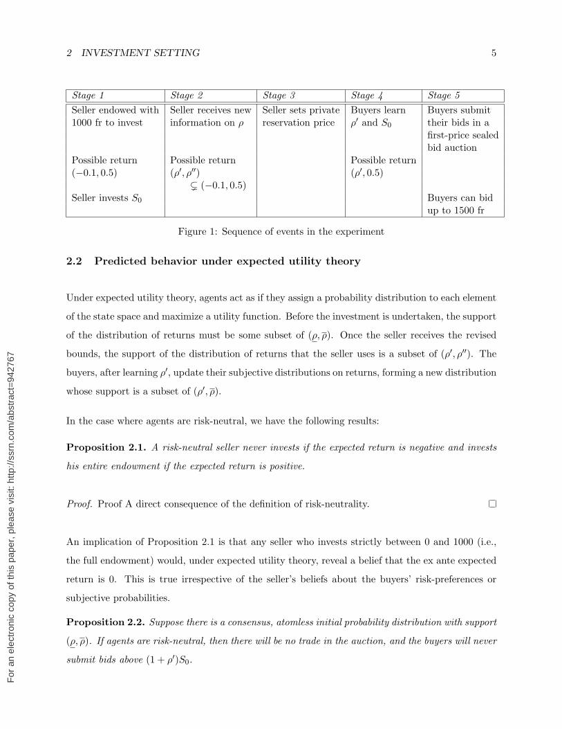
investment by S0. See the first column of Figure 1.

At step 2 (column 2 of Figure 1), the seller receives updated information in the form of new upper

and lower bounds on the possible return. This updated range, which we denote by (ρ′, ρ′′), is

strictly between the original bounds of −10 percent and +50 percent. So (ρ′, ρ′′) ( (ρ, ρ).

At step 3 (column 3), the seller privately decides his reservation price, based on the updated

information. At step 4 (column 4), the buyers learn the updated lower bound ρ′ and the seller’s

investment S0. They do not, however, learn the updated upper bound ρ′′. So at this point, the

seller knows that the return ρ ∈ (ρ′, ρ′′), while the buyers know that ρ ∈ (ρ′, ρ).

At step 5 (column 5), the buyers bid for the asset in a first-price, sealed bid auction. They can bid

up to their endowment of 1500 francs. Thus, trade occurs if the highest bid is above the seller’s

private reservation price, in which case the highest bidder gets the asset and pays the seller his bid.

Otherwise, there is no trade, and the seller keeps the asset. The value of ρ is then announced, and

all the subjects are paid accordingly.

For

an

elec

tron

ic c

opy

of th

is p

aper

, ple

ase

visi

t: ht

tp://

ssrn

.com

/abs

trac

t=94

2767


Stage 1 Stage 2 Stage 3 Stage 4 Stage 5Seller endowed with Seller receives new Seller sets private Buyers learn Buyers submit1000 fr to invest information on ρ reservation price ρ′ and S0 their bids in a

first-price sealedbid auction

Possible return Possible return Possible return(−0.1, 0.5) (ρ′, ρ′′) (ρ′, 0.5)

( (−0.1, 0.5)Seller invests S0 Buyers can bid

up to 1500 fr

Figure 1: Sequence of events in the experiment

2.2 Predicted behavior under expected utility theory

Under expected utility theory, agents act as if they assign a probability distribution to each element

of the state space and maximize a utility function. Before the investment is undertaken, the support

of the distribution of returns must be some subset of (ρ, ρ). Once the seller receives the revised

bounds, the support of the distribution of returns that the seller uses is a subset of (ρ′, ρ′′). The

buyers, after learning ρ′, update their subjective distributions on returns, forming a new distribution

whose support is a subset of (ρ′, ρ).

In the case where agents are risk-neutral, we have the following results:

Proposition 2.1. A risk-neutral seller never invests if the expected return is negative and invests

his entire endowment if the expected return is positive.

Proof. Proof A direct consequence of the definition of risk-neutrality.

An implication of Proposition 2.1 is that any seller who invests strictly between 0 and 1000 (i.e.,

the full endowment) would, under expected utility theory, reveal a belief that the ex ante expected

return is 0. This is true irrespective of the seller’s beliefs about the buyers’ risk-preferences or

subjective probabilities.

Proposition 2.2. Suppose there is a consensus, atomless initial probability distribution with support

(ρ, ρ). If agents are risk-neutral, then there will be no trade in the auction, and the buyers will never

submit bids above (1 + ρ′)S0.

For

an

elec

tron

ic c

opy

of th

is p

aper

, ple

ase

visi

t: ht

tp://

ssrn

.com

/abs

trac

t=94

2767


Proof. Proof After learning the revised upper and lower bounds on the return, the seller forms

a reservation price based on ρ′ and ρ′′, whereas the buyers only know ρ′. If a buyer submits a

bid above (1 + ρ′)S0 and the seller is risk-neutral, then trade occurs only if the bid exceeds the

seller’s private expectation; the latter is the expectation conditional upon all the information in the

economy. That is, a bid above S0(1+ρ′) wins only if it has negative expected value. Consequently,

a risk-neutral buyer will only bid S0(1+ ρ′) or less, and this must be strictly below the risk-neutral

seller’s reservation price. There will therefore be no trade.

Proposition 2.2 provides several tests for risk-neutral expected utility maximization, along with

some generalizations.3 If any buyer in any round makes a bid above ρ′, then this buyer cannot

simultaneously be risk-neutral and believe that the other subjects are risk-neutral. The technical

restriction to atomless distributions with full support rules out situations where buyers can safely

bid more than S0(1 + ρ′) (e.g., if every return between ρ′ and the return implied by the bid has

probability 0). Similarly, any seller setting a reservation price at or below the lower bound would

be a violation of expected utility maximization for a risk-neutral seller.

2.3 Predicted behavior under rational non-probabilistic belief revision

Our non-probabilistic model of belief revision is based on Stecher (2005b), where agents have

incomplete preferences over ambiguous objects. We use here only the assumptions from this model

that are necessary to derive predictions in the current setting.

In particular, we assume that individuals who know ranges of possible returns prefer assets with

unambiguously higher returns. For example, an asset with a return in (0.1, 0.2) is preferred to one

with a return in (0, 0.1). An agent’s preference is indeterminate when intervals overlap. Stecher’s3The no-trade prediction of Proposition 2.2 holds whenever subjects have homogeneous risk-aversion and start

with a common prior. Thus, under the Harsanyi doctrine (Harsanyi 1967, 1968a,b), there should be no trade under

homogeneous risk-preferences; see also Aumann (1976). When agents are heterogeneous in their risk-aversion, trade

can occur, but only in highly restricted ways; in particular, the least risk-averse agent should win every auction.

Similarly, when agents have diffuse priors, the agent with the highest expected return should win every auction.

There was no evidence of such trading behavior in our data.

For

an

elec

tron

ic c

opy

of th

is p

aper

, ple

ase

visi

t: ht

tp://

ssrn

.com

/abs

trac

t=94

2767


model can be shown to induce an interval ordering on the set of alternatives.4

A rational seller in this setting can invest anything between 0 and 1000 francs, and can set his

reservation price anywhere between (1 + ρ′)S0 and (1 + ρ′′)S0. This is because the seller initially

knows that the return can be positive, negative, or zero; if the seller does not form probabilistic

beliefs, his preference for this asset is indeterminate. Similarly, his updated belief is that the value

of the asset lies somewhere between (1+ρ′)S0 and (1+ρ′′)S0, but the seller cannot specify a unique

expectation in this range.

The fact that the seller cannot form a unique expectation completely alters the optimal strategy for

the buyers: the buyers can now rationally bid anything in the interval from (1+ ρ′)S0 to (1+ ρ)S0.

Recall that under the expected utility model, the seller would privately set a reservation price at the

expected value of the asset, so that any buyer who submits a potentially winning bid would have

a negative expected return. In the non-probabilistic setting, however, there is no unique expected

value available to the seller, so buyers can justify making potentially winning bids. Moreover, since

the seller can rationally set his reservation price to (1 + ρ′)S0 (again in contrast with the expected

utility setting, where the reservation price must be strictly above this lower bound), any bid below

this ex post lower bound is dominated by a bid at (1 + ρ′)S0. A buyer bidding less than this can

never expect to win the asset from a rational seller, while a buyer bidding exactly this amount has

some chance of purchasing the asset, and if so will purchase an asset guaranteed to make a positive

return (though one that can become arbitrarily small).

The argument stated above shows the following:

Proposition 2.3. Suppose that the agents do not form subjective beliefs and have incomplete pref-

erences, which are increasing over non-overlapping possible payoffs. Then the seller’s reservation

price will belong to the interval [(1+ρ′)S0, (1+ρ′′)S0], and the buyers’ bids will belong to the interval

[(1 + ρ′)S0, (1 + ρ)S0).4For more on interval orders, see Fishburn (1970). Under some circumstances, the semiorders of Luce (1956) also

can be mapped to interval orders, so the results here can generalize to settings with complete preferences but with

intransitive indifference. The approaches closest to ours are Gilboa and Schmeidler (1989) and Bewley (2002). But

Gilboa and Schmeidler assume maximin preferences (that is, their agents always maximize the worst-case scenario),

while Bewley assumes an inertia bias (so that agents do not trade except for something unambiguously better).

For

an

elec

tron

ic c

opy

of th

is p

aper

, ple

ase

visi

t: ht

tp://

ssrn

.com

/abs

trac

t=94

2767


Figure 2: Range of possible bids

Remark. Proposition 2.3 indicates that trade can occur, but trade still need not occur. The inde-

terminacy of the seller’s reservation price makes trade possible, but cannot guarantee trade.

A direct consequence of Proposition 2.3 is the following:

Corollary 2.1. Under the assumptions of Proposition 2.3, if trade occurs, the market price will

belong to the same interval as the buyers’ possible bids, namely, [(1 + ρ′)S0, (1 + ρ)S0).

Proof. Proof A rational seller’s reservation price must be at least (1 + ρ′)S0, so no trade can occur

below this price. A rational buyer’s bid must be below (1 + ρ)S0, since the asset is guaranteed

to return less than this amount. Between the seller’s lowest possible bid and the buyers’ highest

possible price, behavior is indeterminate, so trade is possible.

Figure 2 presents an overview of the possible bids and possible reservation prices under each model.

For

an

elec

tron

ic c

opy

of th

is p

aper

, ple

ase

visi

t: ht

tp://

ssrn

.com

/abs

trac

t=94

2767


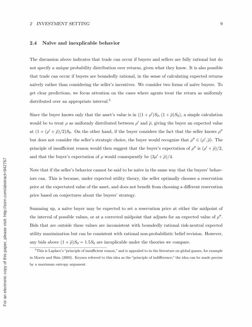
2.4 Naıve and inexplicable behavior

The discussion above indicates that trade can occur if buyers and sellers are fully rational but do

not specify a unique probability distribution over returns, given what they know. It is also possible

that trade can occur if buyers are boundedly rational, in the sense of calculating expected returns

naıvely rather than considering the seller’s incentives. We consider two forms of naıve buyers. To

get clear predictions, we focus attention on the cases where agents treat the return as uniformly

distributed over an appropriate interval.5

Since the buyer knows only that the asset’s value is in ((1 + ρ′)S0, (1 + ρ)S0), a simple calculation

would be to treat ρ as uniformly distributed between ρ′ and ρ, giving the buyer an expected value

at (1 + (ρ′ + ρ)/2)S0. On the other hand, if the buyer considers the fact that the seller knows ρ′′

but does not consider the seller’s strategic choice, the buyer would recognize that ρ′′ ∈ (ρ′, ρ). The

principle of insufficient reason would then suggest that the buyer’s expectation of ρ′′ is (ρ′ + ρ)/2,

and that the buyer’s expectation of ρ would consequently be (3ρ′ + ρ)/4.

Note that if the seller’s behavior cannot be said to be naıve in the same way that the buyers’ behav-

iors can. This is because, under expected utility theory, the seller optimally chooses a reservation

price at the expectated value of the asset, and does not benefit from choosing a different reservation

price based on conjectures about the buyers’ strategy.

Summing up, a naıve buyer may be expected to set a reservation price at either the midpoint of

the interval of possible values, or at a corrected midpoint that adjusts for an expected value of ρ′′.

Bids that are outside these values are inconsistent with boundedly rational risk-neutral expected

utility maximization but can be consistent with rational non-probabilistic belief revision. However,

any bids above (1 + ρ)S0 = 1.5S0 are inexplicable under the theories we compare.5This is Laplace’s“principle of insufficient reason,”and is appealed to in the literature on global games, for example

in Morris and Shin (2003). Keynes referred to this idea as the “principle of indifference;” the idea can be made precise

by a maximum entropy argument.

For

an

elec

tron

ic c

opy

of th

is p

aper

, ple

ase

visi

t: ht

tp://

ssrn

.com

/abs

trac

t=94

2767

3 EXPERIMENTAL PROCEDURE 10

3 Experimental Procedure

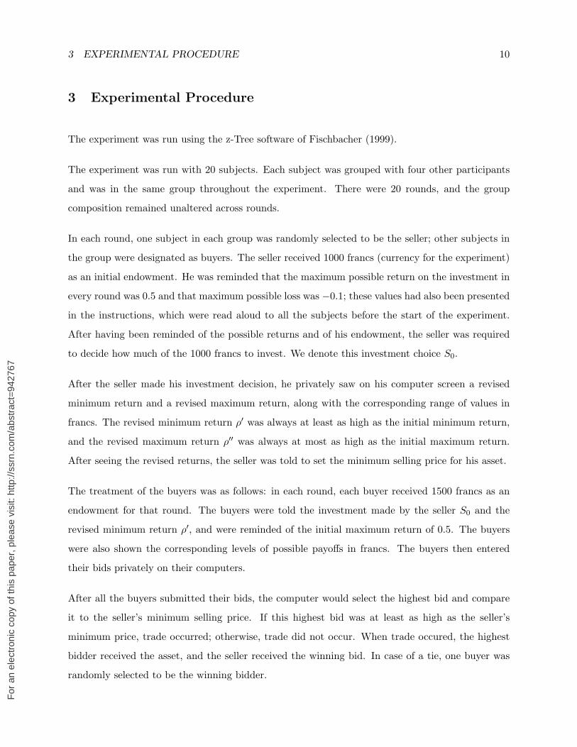
The experiment was run using the z-Tree software of Fischbacher (1999).

The experiment was run with 20 subjects. Each subject was grouped with four other participants

and was in the same group throughout the experiment. There were 20 rounds, and the group

composition remained unaltered across rounds.

In each round, one subject in each group was randomly selected to be the seller; other subjects in

the group were designated as buyers. The seller received 1000 francs (currency for the experiment)

as an initial endowment. He was reminded that the maximum possible return on the investment in

every round was 0.5 and that maximum possible loss was −0.1; these values had also been presented

in the instructions, which were read aloud to all the subjects before the start of the experiment.

After having been reminded of the possible returns and of his endowment, the seller was required

to decide how much of the 1000 francs to invest. We denote this investment choice S0.

After the seller made his investment decision, he privately saw on his computer screen a revised

minimum return and a revised maximum return, along with the corresponding range of values in

francs. The revised minimum return ρ′ was always at least as high as the initial minimum return,

and the revised maximum return ρ′′ was always at most as high as the initial maximum return.

After seeing the revised returns, the seller was told to set the minimum selling price for his asset.

The treatment of the buyers was as follows: in each round, each buyer received 1500 francs as an

endowment for that round. The buyers were told the investment made by the seller S0 and the

revised minimum return ρ′, and were reminded of the initial maximum return of 0.5. The buyers

were also shown the corresponding levels of possible payoffs in francs. The buyers then entered

their bids privately on their computers.

After all the buyers submitted their bids, the computer would select the highest bid and compare

it to the seller’s minimum selling price. If this highest bid was at least as high as the seller’s

minimum price, trade occurred; otherwise, trade did not occur. When trade occured, the highest

bidder received the asset, and the seller received the winning bid. In case of a tie, one buyer was

randomly selected to be the winning bidder.

For

an

elec

tron

ic c

opy

of th

is p

aper

, ple

ase

visi

t: ht

tp://

ssrn

.com

/abs

trac

t=94

2767

3 EXPERIMENTAL PROCEDURE 11

The true return was determined and payoffs were calculated as follows: If trade did not occur,

seller’s payoff was set to 1000 francs − the seller’s investment + the actual payoff from the asset −

the minimum possible ending balance (900 francs):

Seller’s Payoff if No Trade = (1000− S0) + (1 + ρ)S0 − 900 = 100 + ρS0. (1)

If trade occured, seller’s payoff was set to 1,000 francs − the seller’s investment + the selling price

− the minimum possible ending balance (900 francs):

Seller’s Payoff if Trade = (1000− S0) + Highest Bid − 900 = 100 + Highest Bid − S0. (2)

Payoffs to the buyers were calculated analogously: if trade did not occur, each buyer’s payoff was

set to 1500 francs − the minimum possible ending balance (900 francs). If trade did occur, the

payoff to the winning buyer was 1,500 francs − the purchase price + the actual payoff from the

asset − the minimum possible ending balance (900 francs); the payoffs to the other buyers was

1,500 francs − the minimum possible ending balance (900 francs) = 600 francs:

Highest Bidder’s Payoff if Trade = 1500− Highest Bid + (1 + ρ)S0 − 900

= 600− Highest Bid + (1 + ρ)S0. (3)

Other Buyers’ Payoffs if Trade = All Buyers’ Payoffs if No Trade = 1500− 900 = 600. (4)

Note that the minimum possible payoff to the seller assumes that the seller does not sell the asset

for a return below the ex ante lower bound of −10%. Analogously, the minimum possible payoff

to the buyers assumes the buyers do not bid above the ex ante upper bound of 50%. The earnings

from each round were put into a bank account and were unavailable for use in trade in subsequent

rounds. At the end of the experiment, each subject’s total earnings were converted to Canadian

dollars, at the exchange rate of 4 francs to 1¢.

An experimenter read the instructions aloud to the subjects, while the subjects followed their own

copies of the instructions. The experimenter then asked the subjects to answer written questions

about the experiment. The CIRANO Research Institute in Montreal recruited the subjects and

ran the experiment.

In order to generate returns from an unknown probability distribution, we used generated revised

bounds and the actual return using quantum bits (qbits). This procedure gave us a distribution

For

an

elec

tron

ic c

opy

of th

is p

aper

, ple

ase

visi

t: ht

tp://

ssrn

.com

/abs

trac

t=94

2767

4 RESULTS 12

of returns unknown even to the experimenters. The procedure works as follows: each qbit was

determined by firing a photon at a semi-transparent mirror; a device then attempted to determine

whether the photon had passed through the barrier. If the photon was detected, a qbit was set

equal to 1; otherwise, it was set equal to zero. A string of 8 qbits constructed in this way was

converted to a real number.6

4 Results

The experiment produced 71 rounds across the four groups of subjects (referred to henceforth

as group-rounds).7 The sellers’ average investment was typically not all or nothing: only one

group-round (1.4%) had nothing invested, while in 14 group-rounds (19.7%), the sellers invested

everything.8 Thus, 79.9% of investment decisions were inconsistent with risk-neutral expected

utility maximization but consistent with rational non-probabilistic decision making.

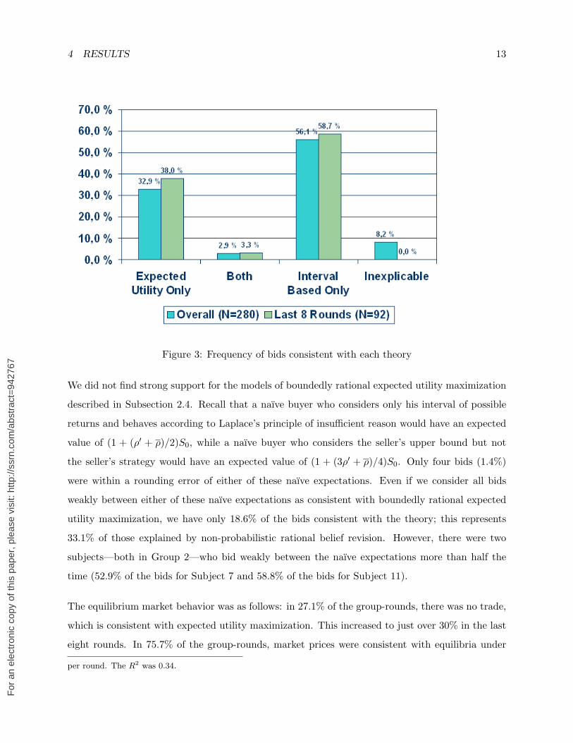
Among the buyers, 32.9% of the bids were at or below the ex post lower bound (1+ρ′)S0, and were

thus in a range consistent with expected utility theory. In the last eight rounds of the experiments,

this increased to 38.0%. Only 2.9% of the bids were exactly at the ex post lower bound (the only

point consistent with both theories); this did not change significantly in the last eight rounds of the

experiment. We observed 56.1% of the bids between the ex post lower bound (1 + ρ′)S0 and the ex

ante upper bound 1.5S0, consistent with rational non-probabilistic belief revision. The remaining

bids were inexplicable (above the ex ante upper bound). All of the inexplicable bids occurred during

the first 12 rounds. See Figure 3.6Cristian Calude provided us with the quantum bits. The probability that a qbit equals 1 is almost surely

uncomputable. There is also reason to question whether a string of qbits obeys even a weak law of large numbers;

see Calude and Zamfirescu (1998).7A data entry error in Round 12 for Group 1 produced a revised lower bound on the return that exceeded the

revised upper bound. Consequently, the last nine rounds for Group 1 were excluded from the analysis. Inclusion of

these data do not substantively change the results.8The average investment was 606.55 francs. It was over 500 francs in all but the first round (where average

investment was 444.75 francs), and under 900 francs in all but the last round (where it was 923.75), and had a general

updtrend through the experiment. A simple OLS regression of average contribution on the round number had an

intercept of 553.25 francs and a slope of 13.12 francs, indicating that average investment typically rose 13.12 francs

For

an

elec

tron

ic c

opy

of th

is p

aper

, ple

ase

visi

t: ht

tp://

ssrn

.com

/abs

trac

t=94

2767

4 RESULTS 13

Figure 3: Frequency of bids consistent with each theory

We did not find strong support for the models of boundedly rational expected utility maximization

described in Subsection 2.4. Recall that a naıve buyer who considers only his interval of possible

returns and behaves according to Laplace’s principle of insufficient reason would have an expected

value of (1 + (ρ′ + ρ)/2)S0, while a naıve buyer who considers the seller’s upper bound but not

the seller’s strategy would have an expected value of (1 + (3ρ′ + ρ)/4)S0. Only four bids (1.4%)

were within a rounding error of either of these naıve expectations. Even if we consider all bids

weakly between either of these naıve expectations as consistent with boundedly rational expected

utility maximization, we have only 18.6% of the bids consistent with the theory; this represents

33.1% of those explained by non-probabilistic rational belief revision. However, there were two

subjects—both in Group 2—who bid weakly between the naıve expectations more than half the

time (52.9% of the bids for Subject 7 and 58.8% of the bids for Subject 11).

The equilibrium market behavior was as follows: in 27.1% of the group-rounds, there was no trade,

which is consistent with expected utility maximization. This increased to just over 30% in the last

eight rounds. In 75.7% of the group-rounds, market prices were consistent with equilibria under

per round. The R2 was 0.34.

For

an

elec

tron

ic c

opy

of th

is p

aper

, ple

ase

visi

t: ht

tp://

ssrn

.com

/abs

trac

t=94

2767

5 CONCLUSION 14

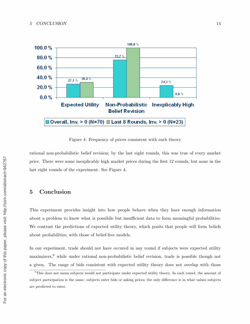
Figure 4: Frequency of prices consistent with each theory

rational non-probabilistic belief revision; by the last eight rounds, this was true of every market

price. There were some inexplicably high market prices during the first 12 rounds, but none in the

last eight rounds of the experiment. See Figure 4.

5 Conclusion

This experiment provides insight into how people behave when they have enough information

about a problem to know what is possibile but insufficient data to form meaningful probabilities.

We contrast the predictions of expected utility theory, which posits that people will form beliefs

about probabilities, with those of belief-free models.

In our experiment, trade should not have occured in any round if subjects were expected utility

maximizers,9 while under rational non-probabilistic belief revision, trade is possible though not

a given. The range of bids consistent with expected utility theory does not overlap with those9This does not mean subjects would not participate under expected utility theory. In each round, the amount of

subject participation is the same: subjects enter bids or asking prices; the only difference is in what values subjects

are predicted to enter.

For

an

elec

tron

ic c

opy

of th

is p

aper

, ple

ase

visi

t: ht

tp://

ssrn

.com

/abs

trac

t=94

2767

REFERENCES 15

consistent with rational non-probabilistic belief revision. Additionally, there were some possible

bids that would be inconsistent with either model, and some focal bids suggestive of boundedly

rational decision-making. Thus, our set-up gave us the ability to make clear distinctions between

the models we were testing and to reject both models.

Approximately 30% of our buyers made bids consistent only with expected utility theory, while

almost 60% were consistent only with non-probabilistic belief revision. There was not strong support

for a naıve model of boundedly rational expected utility maximization, but in the early rounds there

were some bids that were inexplicable under either theory.

The results point to an explanation for the findings of Chen and Plott (1998), who study behavior

in first-price sealed bid auction experiments. Chen and Plott find that their subjects behave con-

sistently with the predictions of game theory, and thus seem to be rational, with the sole exception

being their formation of beliefs. They attribute subjects’ behavior to a form of “limited rational-

ity,”10 and suggest that the answer may lie in a belief-free model. Our results are largely consistent

with those of Chen and Plott, and provide evidence that rational non-probabilistic models can

explain behavior that remains paradoxical under traditional expected utility theory.

References

Carlos E Alchourron, Peter Gardenfors, and David Makinson. On the logic of theory change: Partial meet

contraction and revision functions. Journal of Symbolic Logic, 50(2):510–30, 1985.

Amin H Amershi and Jan H W Stoeckenius. The theory of syndicates and linear sharing rules. Econometrica,

51(5):1407–16, 1983.

Francis J Anscome and Robert J Aumann. A definition of subjective probability. Annals of Mathematical

Statistics, 34(1):199–205, 1963.

Robert J Aumann. Agreeing to disagree. Annals of Statistics, 4(6):1236–9, 1976.

Truman F Bewley. Knightian decision theory. Part I. Decisions in Economics and Finance, 25(2):79–110,

2002.

Lawrence E Blume, David A Easley, and Joseph Y Halpern. Redoing the foundations of decision theory.

Technical report, Cornell University, 2005.

10Their notion of limited rationality is different from the one in the literature, e.g. Lipman (1991).

For

an

elec

tron

ic c

opy

of th

is p

aper

, ple

ase

visi

t: ht

tp://

ssrn

.com

/abs

trac

t=94

2767

REFERENCES 16

Cristian S Calude and Tudor Zamfirescu. The typical number is a lexicon. New Zealand Journal of Mathe-

matics, 27:7–13, 1998.

Kay-Yut Chen and Charles R Plott. Nonlinear behavior in sealed bid first price auctions. Games and

Economic Behavior, 25(1):34–78, 1998.

Eddie Dekel, Barton L Lipman, and Aldo Rustichini. Standard state-space models preclude unawareness.

Econometrica, 66(1):159–73, 1998.

David Easley and Aldo Rustichini. Choice without beliefs. Econometrica, 67(5):1157–84, 1999.

Ronald Fagin and Joseph Y Halpern. Belief, awareness, and limited reasoning. Artificial Intelligence, 34:

39–76, 1988.

Urs Fischbacher. z-Tree—Zurich toolbox for readymade economics experiments, experimenter’s manual.

Working Paper 21, Institute for Empirical Research in Economics, University of Zurich, 1999.

Peter C Fishburn. Intransitive indifference with unequal indifference intervals. Journal of Mathematical

Psychology, 7(1):144–9, 1970.

John D Geanakoplos and Herakles M Polemarchakis. We cannot disagree forever. Journal of Economic

Theory, 28(1):192–200, 1982.

John Geanokoplos. Game theory without partitions, and applications to speculation and consensus. Cowles

Foundation Discussion Paper 914, Yale University, 1989.

Itzhak Gilboa and David Schmeidler. Maxmin expected utility with non-unique prior. Journal of Mathe-

matical Economics, 18(2):141–53, 1989.

John C Harsanyi. Games with incomplete information played by “Bayesian” players, I–III. Part I. The basic

model. Management Science, 14(3):159–82, 1967.

John C Harsanyi. Games with incomplete information played by “Bayesian” players, I–III. Part II. Bayesian

equilibrium points. Management Science, 14(5):320–34, 1968a.

John C Harsanyi. Games with incomplete information played by “Bayesian” players, I–III. Part III. The

basic probability distribution of the game. Management Science, 14(7):486–502, 1968b.

Edi Karni. Subjective expected utility without states of the world. Technical report, Johns Hopkins Univer-

sity, August 2005.

Bernard O Koopman. The axioms and algebra of intuitive probability. Annals of Mathematics, 41(2):269–92,

1940a.

Bernard O Koopman. Intuitive probabilities and sequences. Annals of Mathematics, 42(1):169–87, 1941.

Bernard O Koopman. The bases of probability. Bulletin of the American Mathematical Society, 46:763–74,

1940b.

For

an

elec

tron

ic c

opy

of th

is p

aper

, ple

ase

visi

t: ht

tp://

ssrn

.com

/abs

trac

t=94

2767

REFERENCES 17

Barton L Lipman. How to decide how to decide how to . . .: Modeling limited rationality. Econometrica, 59

(4):1105–25, 1991.

R Duncan Luce. Semiorders and a theory of utility discrimination. Econometrica, 24(2):178–91, 1956.

R Duncan Luce. Individual Choice Behavior. Wiley, 1959.

Stephen Morris. The logic of belief and belief change: A decision theoretic approach. Journal of Economic

Theory, 69(1):1–23, 1996.

Stephen Morris and Hyun Song Shin. Global games: Theory and applications. In Mathias Dewatripont,

Lars Peter Hansen, and Stephen J Turnovsky, editors, Advances in Economics and Econometrics,

volume 1, pages 56–114, 2003.

Donald G Saari. The profile structure for Luce’s choice axiom. Journal of Mathematical Psychology, 49(3):

226–53, 2005.

L James Savage. The Foundations of Statistics. Wiley, 1954.

Hyun Song Shin. Logical structure of common knowledge. Journal of Economic Theory, 60(1):1–13, 1993.

Jack Douglas Stecher. Decisions under subjective information. In Ron van der Meyden, editor, Proceedings

of the 10th Conference on Theoretical Aspects of Rationality and Knowledge, pages 150–7. National

University of Singapore, 2005a.

Jack Douglas Stecher. Existence of approximate social welfare. Technical report, Available at SSRN:

http://ssrn.com/abstract=870865, 2005b.

Robert Wilson. The theory of syndicates. Econometrica, 36(1):119–32, 1968.

For

an

elec

tron

ic c

opy

of th

is p

aper

, ple

ase

visi

t: ht

tp://

ssrn

.com

/abs

trac

t=94

2767

1

Instructions This is a computerized experiment in the economics of decision-making. This experiment will last approximately one hour. To make a profit, you will trade a financial asset, which may lose or gain money. At the end of the experiment, we will pay you a show-up fee of $10 plus any profits you will have made. We will pay you in cash, privately, immediately after the experiment ends. You must sign and date a compensation receipt form in order to receive your payment. There are some rules you must follow:

(1) Do not talk to others at any time during the experiment. (2) If you have any questions during the experiment, please raise your hand. An

experimenter will come to your location and answer your questions. You are free to withdraw from the experiment at any time, for any reason. If you choose to do so, please raise your hand. In this case, you will be paid your $10 show-up fee as you leave.

Grouping of the Participants The computer will assign you to a group with four other participants. There are 20 rounds of this experiment. You will be in the same group through all 20 rounds. At the beginning of each round, the computer will select one person from your group as a seller for that round; the other four members of your group will be buyers for that round. In the next round, the computer may select any member of your group as the new seller. If you are the seller, you will be given 1,000 francs of currency at the beginning of the round. Otherwise, if you are a buyer, you will be given 1,500 francs of currency at the beginning of the round. The computer will tell you whether you are a buyer or a seller.

Seller’s Investment Decision If you are a seller, you will see the following table on your screen:

Minimum Return -10%

Maximum Return +50%

Your Investment FR________

The minimum possible return will always be -10% of your investment. That is, the worst that could happen in any round is that you could lose 10% of your investment. The maximum possible return will always be 50%. That is, the best that could happen in any round is that you could gain 50% of what you invest. You may invest as much of the 1,000 francs as you like. The third line in the above table shows where you will enter the amount you wish to invest.

For

an

elec

tron

ic c

opy

of th

is p

aper

, ple

ase

visi

t: ht

tp://

ssrn

.com

/abs

trac

t=94

2767

2

Example 1 Suppose you decide to invest 500 francs. Then your minimum possible payoff is 450 francs. This is calculated as follows:

Your investment 500 francs Less: 10% of your investment 50 francs

Minimum payoff 450 francs Your maximum possible payoff is 750 francs. This is calculated as follows:

Your investment 500 francs Add: 50% of your investment 250 francs

Maximum payoff 750 francs Remember that the true return will be somewhere between the minimum and maximum returns, so your true payoff will be between the minimum and maximum payoffs.

Seller’s Minimum Price If you are a seller, then after you enter your investment, you will see the following table on your screen. Only you will see this table.

Revised Minimum Return (in percent)

Revised Minimum Payoff (in francs)

Revised Maximum Return (in percent)

Revised Maximum Payoff (in francs)

Minimum price for which you are willing to sell your asset

FR________

This table shows your updated minimum and maximum payoffs. Initially, you were told that the return would lie somewhere between -10% and +50%. When you see the above screen, you will know that the true return will lie somewhere between the revised minimum return and the revised maximum return. In the fifth row of the above table, you will enter the minimum price for which you are willing to sell the asset. Example 2 Suppose you decide to invest 100 francs, and that you later learn that the revised minimum return is -5%. Then revised minimum payoff is 95 francs. This is calculated as follows:

Your investment 100 francs Less: 5% of your investment 5 francs

Revised minimum payoff 95 francs If the revised maximum return is 30%, then the revised maximum payoff is 130 francs. This is calculated as follows:

Your investment 100 francs Add: 30% of your investment 30 francs

Revised maximum payoff 130 francs The screen you will see in this case is:

For

an

elec

tron

ic c

opy

of th

is p

aper

, ple

ase

visi

t: ht

tp://

ssrn

.com

/abs

trac

t=94

2767

3

Revised Minimum Return (in percent) -5%

Revised Minimum Payoff (in francs) 95 francs

Revised Maximum Return (in percent) 30%

Revised Maximum Payoff (in francs) 130 francs

Minimum price for which you are willing to sell your asset

FR________

Buyer’s Bidding Decision If you are a buyer, you will see the following table on your screen after the seller privately sees the revised information and privately sets the minimum selling price:

Seller’s Investment (in francs)

Minimum Return (in percent)

Minimum Payoff (in francs)

Maximum Return (in percent) +50%

Maximum Payoff (in francs)

Your Bid FR ________

The first line in the above table states how many francs the seller has invested. The second line is the seller’s revised minimum return. That is, you will learn the same minimum possible return that the seller learns. The third line converts this minimum return into a payoff. Line four tells you the initial maximum return—that is, what the seller was told, before making the investment, that the highest return could be. You will not learn the seller’s revised maximum return. The initial maximum return is always 50%. Line five converts this 50% into a payoff. On the last line of the above table, you will enter what you are willing to pay for the asset. You may enter any amount of your 1,500 francs for that round. Example 3: Suppose you see the following numbers on your screen:

Seller’s Investment (in francs) 1000 francs

Minimum Return (in percent) 5%

Minimum Payoff (in francs) 1050 francs

For

an

elec

tron

ic c

opy

of th

is p

aper

, ple

ase

visi

t: ht

tp://

ssrn

.com

/abs

trac

t=94

2767

4

Maximum Return (in percent) 50%

Maximum Payoff (in francs) 1500 francs

Your Bid (in francs) FR ________

The revised minimum payoff of 1050 francs is calculated as:

Seller’s investment 1000 francs Add: 5% of the investment 50 francs

Revised minimum payoff 1050 francs The maximum payoff is calculated as

Seller’s investment 1000 francs Add: 50% of the investment 500 francs

Maximum payoff 1500 francs

How the market price will be determined After all four buyers in your group submit their bids, the computer decides whether trade will occur. If the highest bid is at least the minimum price the seller will accept, then trade will occur; otherwise, no trade will occur. It trade occurs, the asset will be sold to the highest bidder. If two or more buyers have this highest bid, then the computer will randomly select one of these buyers and sell the asset to the selected buyer. The computer will then determine the return and the payoff. This will be between the revised minimum and the revised maximum.

Determination of Profits After determining the true payoff, the computer will calculate the profit for all the members in your group. If you are a buyer, you will see the following screen:

Trade occurred / did not occur

Actual return (in percent)

Actual payoff (in francs)

Your bid (in francs)

Highest bid (in francs)

Initial balance (in francs) 1500 francs

Less: Your bid, if you bought the asset (in francs)

For

an

elec

tron

ic c

opy

of th

is p

aper

, ple

ase

visi

t: ht

tp://

ssrn

.com

/abs

trac

t=94

2767

5

Add: Actual payoff, if you bought the asset (in francs)

Less: Smallest possible ending balance (in francs) 900 francs

Net profit for this round (in francs)

Total profit to date

If you are a seller, you will see the following screen:

Trade occurred / did not occur

Actual return (in percent)

Actual payoff (in francs)

Your minimum acceptable selling price (in francs)

Highest bid (in francs)


Less: Your investment (in francs)

Add: Actual payoff, if trade did not occur (in francs)

Add: Highest bid, if trade occurred (in francs)


Net profit for this round (in francs)

Total profit to date

Profits are determined in the following way:

If you are the seller and you do not sell the asset, your profit will be 1000 francs – francs invested + the actual payoff from the asset – the minimum possible ending balance (900 francs). If you are the seller and you do sell the asset, your profit will be 1,000 francs – francs invested + selling price – the minimum possible ending balance (900 francs). If you are a buyer and you do not purchase the asset, your profit will be 1,500 francs – the minimum possible ending balance (900 francs) = 600 francs. If you are a buyer and you do purchase the asset, your profit will be 1,500 francs – your purchase price + the actual payoff from the asset – the minimum possible ending balance (900 francs).

For

an

elec

tron

ic c

opy

of th

is p

aper

, ple

ase

visi

t: ht

tp://

ssrn

.com

/abs

trac

t=94

2767

6

Example 4 Suppose the seller’s investment is 500 francs and the screen for a buyer shows:

Trade occurred

Actual return (in percent) 30 %

Actual payoff (in francs) 650 francs

Your bid (in francs) 600 francs

Highest bid (in francs) 600 francs


Less: Your bid, if you bought the asset (in francs) 600 francs


650 francs


Net profit for this round (in francs) 650 francs

Total profits to date

Since this buyer made the highest bid, he or she bought the asset. The bottom row shows the total profits from this round and all previous rounds. We have left this blank in the example, but you will see this figure during the experiment. The seller’s screen in this case will appear as:

Trade occurred

Actual return (in percent) 30 %


Your minimum acceptable selling price (in francs) 580 francs



Less: Your investment (in francs) 500 francs


Add: Highest bid, if trade occurred (in francs) 600 francs


For

an

elec

tron

ic c

opy

of th

is p

aper

, ple

ase

visi

t: ht

tp://

ssrn

.com

/abs

trac

t=94

2767

7



The bottom row shows the total profits from this round and all previous rounds. We have left this blank in the example, but you will see this figure during the experiment. Example 5 Suppose the seller’s investment is 100 francs and the screen for a buyer shows:

Trade did not occur

Actual return (in percent) 10%


Your bid (in francs) 102 francs



Less: Your bid, if you bought the asset (in francs)





Since this buyer did not make the highest bid, the buyer only had the smallest possible ending balance of 900 francs deducted, leaving him or her with 600 francs for the round. The bottom row shows the total profits from this round and all previous rounds. We have left this blank in the example, but you will see this figure during the experiment. The seller’s screen in this case will appear as:

Trade did not occur

Actual return (in percent) 10%


Your minimum acceptable selling price (in francs) 120 francs



For

an

elec

tron

ic c

opy

of th

is p

aper

, ple

ase

visi

t: ht

tp://

ssrn

.com

/abs

trac

t=94

2767

8

Less: Your investment (in francs) 100 francs


110 francs

Add: Highest bid, if trade occurred (in francs)



Total Profits to date

Since the highest bid was less than the minimum acceptable selling price, trade did not occur. The bottom row shows the total profits from this round and all previous rounds. We have left this blank in the example, but you will see this figure during the experiment.

What You Will Be Paid The profit you accumulate in each round (after deducting the minimum possible payoff of 900 francs) will not be available to you for trading in subsequent rounds. However, your profits from each round will be totaled, and paid to you in dollars at the end of the experiment, at the rate of 4 francs / 1 cent.

Questions Below, please write down your answers to the following questions. In a few minutes, an experimenter will review the correct answers with you.

1. You are the seller. If you invest 850 francs, what is the maximum amount you can lose, and what is the maximum amount you can gain?

2. You are the seller, and your investment is 200 francs. The revised minimum return is -5%, and the revised maximum return is 30%. What are the lowest and highest possible payoffs?

3. You are the buyer, and you learn that the seller invested 600 francs and the (revised) minimum return is -5%. What is the maximum possible payoff?

4. The minimum price for which seller is willing to sell the asset is 700 francs, and highest bid is 689 francs. Will trade occur?

5. Suppose trade does not occur, the seller invested 400 francs, and the actual payoff is 380 francs. What is the seller’s net profit, and what is each buyer’s net profit?

6. Suppose trade occurs, and the seller has invested 600 francs. The highest bid is 650 francs, and the actual payoff is 670 francs. What are the payoffs to the seller, the buyer making the highest bid, and the other buyers?

Decision Making and Trade without ProbabilitiesDecision Making and Trade without Probabilities* Jack...

Documents

Transcript of Decision Making and Trade without ProbabilitiesDecision Making and Trade without Probabilities* Jack...