Dec 20Testability@IITK1 Testability Virendra Singh Indian Institute of Science Bangalore IEP on...

Dec 20 Testability@IITK 1

TestabilityTestability

Virendra SinghIndian Institute of Science

Bangalore

IEP on Digital System Synthesis

At IIT Kanpur


Why Model Faults?Why Model Faults?

I/O function tests inadequate for manufacturing (functionality versus component and interconnect testing)

Real defects (often mechanical) too numerous and often not analyzable

A fault model identifies targets for testing A fault model makes analysis possible Effectiveness measurable by experiments


Some Real Defects in ChipsSome Real Defects in Chips Processing defects

Missing contact windows Parasitic transistors Oxide breakdown . . .

Material defects Bulk defects (cracks, crystal imperfections) Surface impurities (ion migration) . . .

Time-dependent failures Dielectric breakdown Electromigration . . .

Packaging failures Contact degradation Seal leaks . . .

Ref.: M. J. Howes and D. V. Morgan, Reliability and Degradation - Semiconductor Devices and Circuits, Wiley, 1981.


Common Fault ModelsCommon Fault Models

Single stuck-at faults Transistor open and short faults Memory faults PLA faults (stuck-at, cross-point, bridging) Functional faults (processors) Delay faults (transition, path) Analog faults For more details of fault models, see

M. L. Bushnell and V. D. Agrawal, Essentials of Electronic Testing for Digital, Memory and Mixed-Signal VLSI Circuits, Springer, 2000.


Single Stuck-at FaultSingle Stuck-at Fault Three properties define a single stuck-at fault

Only one line is faulty The faulty line is permanently set to 0 or 1 The fault can be at an input or output of a gate

Example: XOR circuit has 12 fault sites ( ) and 24 single stuck-at faults

a

b

c

d

e

f

10

g h i 1

s-a-0j

k

z

0(1)1(0)

1

Test vector for h s-a-0 fault

Good circuit valueFaulty circuit value


Purpose - TestabilityPurpose - Testability Need approximate measure of:

Difficulty of setting internal circuit lines to 0 or 1 by setting primary circuit inputs

Difficulty of observing internal circuit lines by observing primary outputs

Uses: Analysis of difficulty of testing internal

circuit parts – redesign or add special test hardware

Guidance for algorithms computing test patterns – avoid using hard-to-control lines

Estimation of fault coverage Estimation of test vector length


Testability AnalysisTestability Analysis

Involves Circuit Topological analysis, but no test vectors and no search algorithm

Static analysis Linear computational complexity

Otherwise, is pointless – might as well use automatic test-pattern generation and calculate:

Exact fault coverage Exact test vectors


Types of MeasuresTypes of Measures

SCOAP – Sandia Controllability and Observability Analysis Program

Combinational measures: CC0 – Difficulty of setting circuit line to logic 0 CC1 – Difficulty of setting circuit line to logic 1 CO – Difficulty of observing a circuit line

Sequential measures – analogous: SC0 SC1 SO


Range of SCOAP MeasuresRange of SCOAP Measures

Controllabilities – 1 (easiest) to infinity (hardest) Observabilities – 0 (easiest) to infinity (hardest) Combinational measures:

Roughly proportional to # circuit lines that must be set to control or observe given line

Sequential measures: Roughly proportional to # times a flip-flop must

be clocked to control or observe given line


Goldstein’s SCOAP Measures

Goldstein’s SCOAP Measures

AND gate O/P 0 controllability: output_controllability = min (input_controllabilities) + 1 AND gate O/P 1 controllability: output_controllability = (input_controllabilities) + 1 XOR gate O/P controllability

output_controllability = min (controllabilities of each input set) + 1

Fanout Stem observability: or min (some or all fanout branch observabilities)


Controllability Examples

Controllability Examples


More ControllabilityExamples

More ControllabilityExamples


Observability Examples

Observability Examples

To observe a gate input:Observe output and make other input values non-

controlling


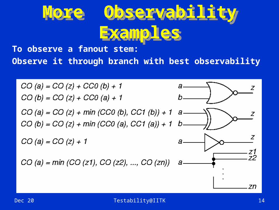
More Observability Examples

More Observability Examples

To observe a fanout stem:Observe it through branch with best observability


BIST MotivationBIST Motivation Useful for field test and diagnosis (less

expensive than a local automatic test equipment)

Software tests for field test and diagnosis: Low hardware fault coverage Low diagnostic resolution Slow to operate

Hardware BIST benefits: Lower system test effort Improved system maintenance and

repair Improved component repair Better diagnosis


Costly Test Problems Alleviated by BIST

Costly Test Problems Alleviated by BIST

Increasing chip logic-to-pin ratio – harder observability

Increasingly dense devices and faster clocks Increasing test generation and application

times Increasing size of test vectors stored in ATE Expensive ATE needed for 1 GHz clocking chips Hard testability insertion – designers unfamiliar

with gate-level logic, since they design at behavioral level

In-circuit testing no longer technically feasible Shortage of test engineers Circuit testing cannot be easily partitioned


Typical Quality Requirements

Typical Quality Requirements

98% single stuck-at fault coverage 100% interconnect fault coverage Reject ratio – 1 in 100,000


Economics – BIST CostsEconomics – BIST Costs Chip area overhead for:

Test controller Hardware pattern generator Hardware response compacter Testing of BIST hardware

Pin overhead -- At least 1 pin needed to activate BIST operation

Performance overhead – extra path delays due to BIST

Yield loss – due to increased chip area or more chips In system because of BIST

Reliability reduction – due to increased area Increased BIST hardware complexity –

happens when BIST hardware is made testable


BIST BenefitsBIST Benefits Faults tested:

Single combinational / sequential stuck-at faults

Delay faults Single stuck-at faults in BIST hardware

BIST benefits Reduced testing and maintenance cost Lower test generation cost Reduced storage / maintenance of test

patterns Simpler and less expensive ATE Can test many units in parallel Shorter test application times Can test at functional system speed


DefinitionsDefinitions BILBO – Built-in logic block observer, extra

hardware added to flip-flops so they can be reconfigured as an LFSR pattern generator or response compacter, a scan chain, or as flip-flops

Concurrent testing – Testing process that detects faults during normal system operation

CUT – Circuit-under-test Exhaustive testing – Apply all possible 2n

patterns to a circuit with n inputs Irreducible polynomial – Boolean polynomial

that cannot be factored LFSR – Linear feedback shift register, hardware

that generates pseudo-random pattern sequence


More DefinitionsMore Definitions Primitive polynomial – Boolean polynomial p

(x) that can be used to compute increasing powers n of xn modulo p (x) to obtain all possible non-zero polynomials of degree less than p (x)

Pseudo-exhaustive testing – Break circuit into small, overlapping blocks and test each exhaustively

Pseudo-random testing – Algorithmic pattern generator that produces a subset of all possible tests with most of the properties of randomly-generated patterns

Signature – Any statistical circuit property distinguishing between bad and good circuits

TPG – Hardware test pattern generator


BIST ProcessBIST Process

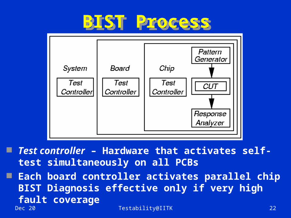
Test controller – Hardware that activates self-test simultaneously on all PCBs

Each board controller activates parallel chip BIST Diagnosis effective only if very high fault coverage


BIST ArchitectureBIST Architecture

Note: BIST cannot test wires and transistors: From PI pins to Input MUX From POs to output pins


BILBO – Works as Both a PG and a RC

BILBO – Works as Both a PG and a RC

Built-in Logic Block Observer (BILBO) -- 4 modes:1. Flip-flop2. LFSR pattern generator3. LFSR response compacter4. Scan chain for flip-flops


Complex BIST ArchitectureComplex BIST Architecture

Testing epoch I: LFSR1 generates tests for CUT1 and CUT2 BILBO2 (LFSR3) compacts CUT1 (CUT2)

Testing epoch II: BILBO2 generates test patterns for CUT3 LFSR3 compacts CUT3 response


Pattern GenerationPattern Generation Store in ROM – too expensive Exhaustive Pseudo-exhaustive Pseudo-random (LFSR) – Preferred method Binary counters – use more hardware than

LFSR Modified counters Test pattern augmentation

LFSR combined with a few patterns in ROM

Hardware diffracter – generates pattern cluster in neighborhood of pattern stored in ROM


Exhaustive Pattern Generation

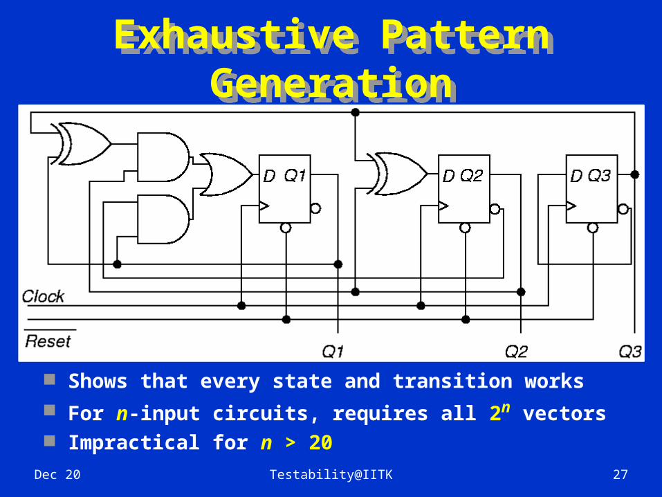
Exhaustive Pattern Generation

Shows that every state and transition works For n-input circuits, requires all 2n vectors Impractical for n > 20


Pseudo-Exhaustive Method

Pseudo-Exhaustive Method

Partition large circuit into fanin cones Backtrace from each PO to PIs influencing it Test fanin cones in parallel

Reduced # of tests from 28 = 256 to 25 x 2 = 64 Incomplete fault coverage


Pseudo-Exhaustive Pattern GenerationPseudo-Exhaustive Pattern Generation


Pseudo-Random Pattern Generation

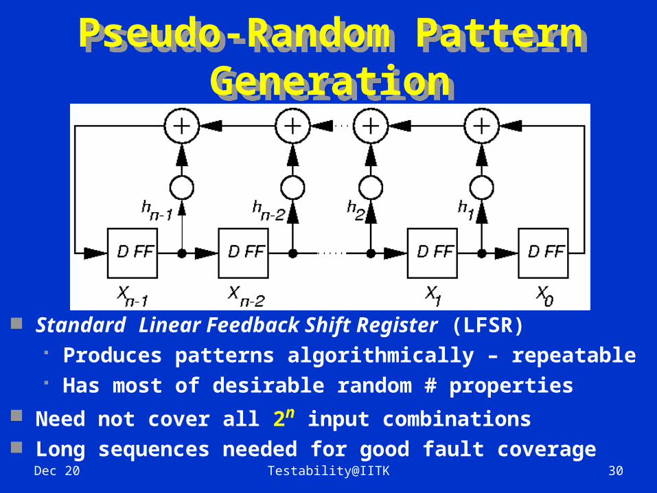
Pseudo-Random Pattern Generation

Standard Linear Feedback Shift Register (LFSR) Produces patterns algorithmically – repeatable Has most of desirable random # properties

Need not cover all 2n input combinations Long sequences needed for good fault coverage


Matrix Equation for Standard LFSR

Matrix Equation for Standard LFSR

X0 (t + 1)

X1 (t + 1)...

Xn-3 (t + 1)

Xn-2 (t + 1)

Xn-1 (t + 1)

10...00

h1

01...00

h2

00...001

…… ………

00...10

hn-2

00...01

hn-1

X0 (t)

X1 (t)...

Xn-3 (t)

Xn-2 (t)

Xn-1 (t)

=

X (t + 1) = Ts X (t) (Ts is companion matrix)


Standard n-Stage LFSR Implementation

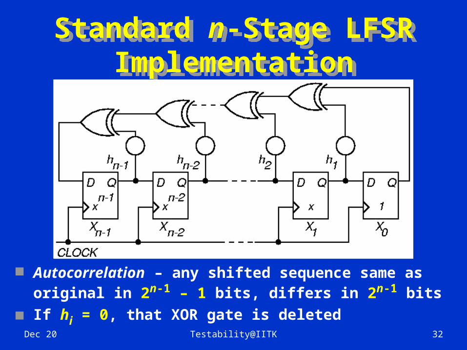
Standard n-Stage LFSR Implementation

Autocorrelation – any shifted sequence same as original in 2n-1 – 1 bits, differs in 2n-1 bits

If hi = 0, that XOR gate is deleted


LFSR TheoryLFSR Theory Cannot initialize to all 0’s – hangs

If X is initial state, progresses through states

X, Ts X, Ts2 X, Ts

3 X, …

Matrix period:

Smallest k such that Tsk = I

k LFSR cycle length

Described by characteristic polynomial:

f (x) = |Ts – I X |

= 1 + h1 x + h2 x2 + … + hn-1 xn-1 + xn


Example External XOR LFSR

Example External XOR LFSR

Characteristic polynomial f (x) = 1 + x + x3

(read taps from right to left)


External XOR LFSRExternal XOR LFSR

Pattern sequence for example LFSR (earlier):

Always have 1 and xn terms in polynomial Never repeat an LFSR pattern more than 1 time

–Repeats same error vector, cancels fault effect

X0 (t + 1)

X1 (t + 1)

X2 (t + 1)

001

101

010

X0 (t)

X1 (t)

X2 (t)

=

X0

X1

X2

100

001

010

101

011

111

110

100

001

…


Generic Modular LFSRGeneric Modular LFSR


Modular Internal XOR LFSRModular Internal XOR LFSR Described by companion matrix Tm = Ts

T

Internal XOR LFSR – XOR gates in between D flip-flops

Equivalent to standard External XOR LFSR With a different state assignment Faster – usually does not matter Same amount of hardware

X (t + 1) = Tm x X (t) f (x) = | Tm – I X |

= 1 + h1 x + h2 x2 + … + hn-1 xn-1 + xn

Right shift – equivalent to multiplying by x, and then dividing by characteristic polynomial and storing the remainder


Modular LFSR MatrixModular LFSR Matrix

X0 (t + 1)

X1 (t + 1)

X2 (t + 1)...

Xn-3 (t + 1)

Xn-2 (t + 1)

Xn-1 (t + 1)

001...000

000...010

010...000

………

………

000...001

1h1h2...

hn-3hn-2hn-1

X0 (t)

X1 (t)

X2 (t)...

Xn-3 (t)

Xn-2 (t)

Xn-1 (t)

=

000...000


Example Modular LFSRExample Modular LFSR

f (x) = 1 + x2 + x7 + x8

Read LFSR tap coefficients from left to right


Primitive PolynomialsPrimitive Polynomials Want LFSR to generate all possible 2n – 1

patterns (except the all-0 pattern) Conditions for this – must have a primitive

polynomial: Monic – coefficient of xn term must be 1

Modular LFSR – all D FF’s must right shift through XOR’s from X0 through X1, …,

through Xn-1, which must feed back directly

to X0

Standard LFSR – all D FF’s must right shift directly from Xn-1 through Xn-2, …, through

X0, which must feed back into Xn-1 through

XORing feedback network


Characteristic polynomial must divide the polynomial 1 – xk for k = 2n – 1, but not for any smaller k value

See Appendix B of book for tables of primitive polynomials

If p (error) = 0.5, no difference between behavior of primitive & non-primitive polynomial

But p (error) is rarely = 0.5 In that case, non-primitive polynomial LFSR takes much longer to stabilize with random properties than primitive polynomial LFSR

Primitive Polynomials (continued)

Primitive Polynomials (continued)


Weighted Pseudo-Random Pattern

Generation


Generation

If p (1) at all PIs is 0.5, pF (1) = 0.58 =

Will need enormous # of random patterns to test a stuck-at 0 fault on F -- LFSR p (1) = 0.5 We must not use an ordinary LFSR to test

this IBM – holds patents on weighted pseudo-

random pattern generator in ATE

1256

255256

1256 pF (0) = 1 – =

f

F s-a-0



Generator


Generator

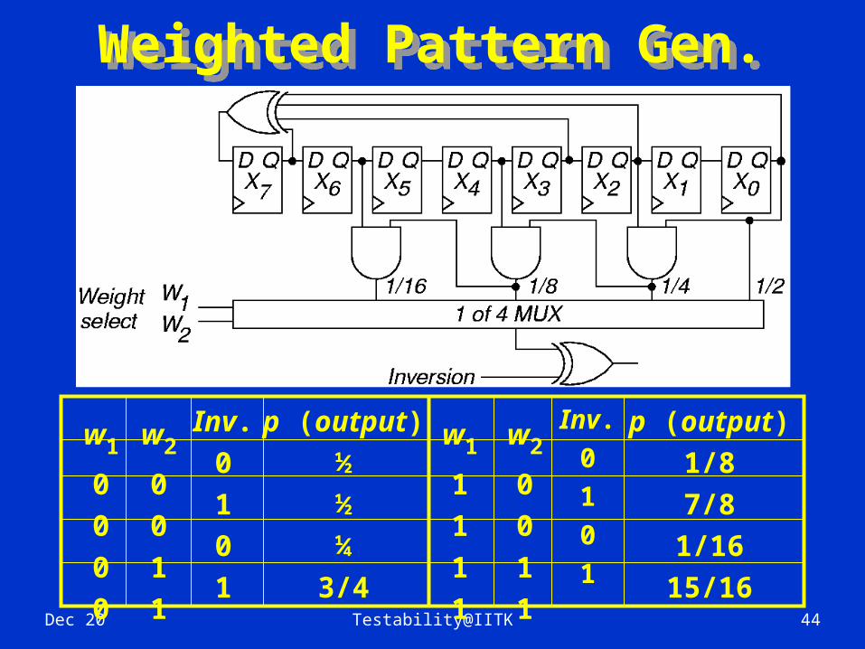
LFSR p (1) = 0.5 Solution: Add programmable weight

selection and complement LFSR bits to get p (1)’s other than 0.5

Need 2-3 weight sets for a typical circuit Weighted pattern generator drastically

shortens pattern length for pseudo-random patterns


Weighted Pattern Gen.Weighted Pattern Gen.

w1

0000

w2

0011

Inv.0101

p (output)½½¼

3/4

w1

1111

w2

0011

p (output)1/87/81/1615/16

Inv.0101


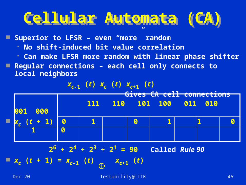
Cellular Automata (CA)Cellular Automata (CA) Superior to LFSR – even “more” random

No shift-induced bit value correlation Can make LFSR more random with linear phase

shifter Regular connections – each cell only connects to

local neighbors

xc-1 (t) xc (t) xc+1 (t) Gives CA cell connections 111 110 101 100 011 010 001 000 xc (t + 1) 0 1 0 1 1 0 1 0

26 + 24 + 23 + 21 = 90 Called Rule 90 xc (t + 1) = xc-1 (t) xc+1 (t)


Response CompactionResponse Compaction

Severe amounts of data in CUT response to LFSR patterns – example: Generate 5 million random patterns CUT has 200 outputs Leads to: 5 million x 200 = 1 billion bits

response Uneconomical to store and check all of these

responses on chip Responses must be compacted


DefinitionsDefinitions Aliasing – Due to information loss, signatures

of good and some bad machines match Compaction – Drastically reduce # bits in

original circuit response – lose information Compression – Reduce # bits in original

circuit response – no information loss – fully invertible (can get back original response)

Signature analysis – Compact good machine response into good machine signature. Actual signature generated during testing, and compared with good machine signature

Transition Count Response Compaction – Count # transitions from 0 1 and 1 0 as a signature


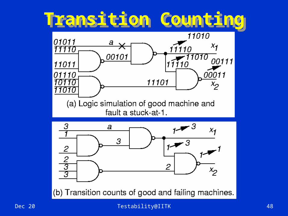
Transition CountingTransition Counting


Transition Counting Details

Transition Counting Details

Transition count:

C (R) = (ri ri-1) for all m primary

outputs

To maximize fault coverage: Make C (R0) – good machine transition

count – as large or as small as possible

i = 1

m


LFSR for Response Compaction

LFSR for Response Compaction

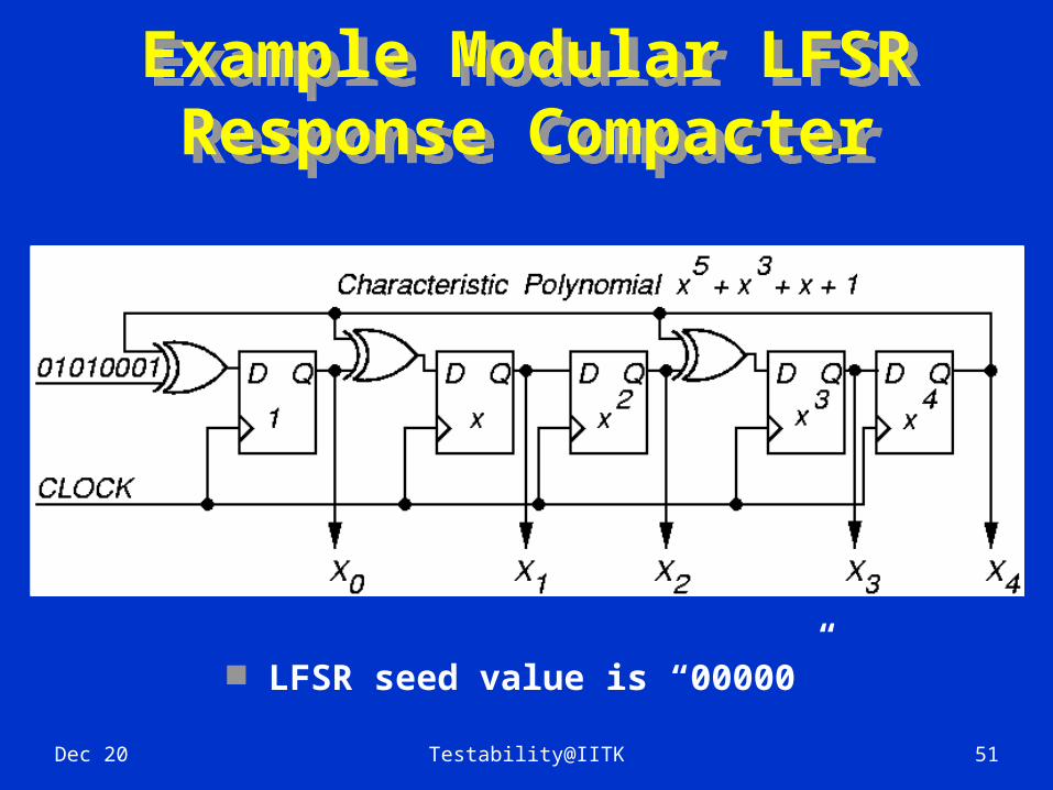
Use cyclic redundancy check code (CRCC) generator (LFSR) for response compacter

Treat data bits from circuit POs to be compacted as a decreasing order coefficient polynomial

CRCC divides the PO polynomial by its characteristic polynomial Leaves remainder of division in LFSR Must initialize LFSR to seed value (usually 0)

before testing After testing – compare signature in LFSR to

known good machine signature Critical: Must compute good machine signature


Example Modular LFSR Response Compacter

Example Modular LFSR Response Compacter

LFSR seed value is “00000”


Polynomial DivisionPolynomial Division

Logic simulation: Remainder = 1 + x2 + x3

0 1 0 1 0 0 0 1

0 x0 + 1 x1 + 0 x2 + 1 x3 + 0 x4 + 0 x5 + 0 x6 + 1 x7

InputsInitial State

10001010

X0

010001111

X1

001000010

X2

000100001

X3

000010101

X4

000001010

........

LogicSimulation:


Symbolic Polynomial Division

Symbolic Polynomial Division

x2

x7

x7

+ 1

+ x5

x5

x5

+ x3

+ x3

+ x3

x3

+ x2

+ x2

+ x2

+ x

+ x

+ x + 1

+ 1

x5 + x3 + x + 1

remainder

Remainder matches that from logic simulationof the response compacter!


Multiple-Input Signature Register

(MISR)

Multiple-Input Signature Register

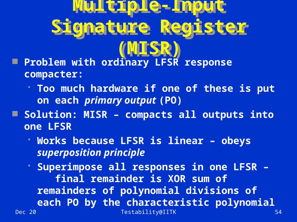
(MISR) Problem with ordinary LFSR response

compacter: Too much hardware if one of these is put

on each primary output (PO) Solution: MISR – compacts all outputs into

one LFSR Works because LFSR is linear – obeys

superposition principle Superimpose all responses in one LFSR –

final remainder is XOR sum of remainders of polynomial divisions of each PO by the characteristic polynomial


MISR Matrix EquationMISR Matrix Equation

di (t) – output response on POi at time t

X0 (t + 1)

X1 (t + 1)...

Xn-3 (t + 1)

Xn-2 (t + 1)

Xn-1 (t + 1)

10...00

h1

00...001

……

………

00...10

hn-2

00...01

hn-1

X0 (t)

X1 (t)...

Xn-3 (t)

Xn-2 (t)

Xn-1 (t)

=

d0 (t)

d1 (t)...

dn-3 (t)

dn-2 (t)

dn-1 (t)

+


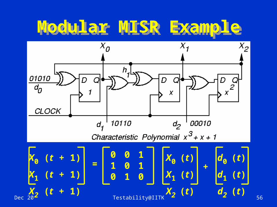
Modular MISR ExampleModular MISR Example

X0 (t + 1)

X1 (t + 1)

X2 (t + 1)

001

010

110

=X0 (t)

X1 (t)

X2 (t)

d0 (t)

d1 (t)

d2 (t)

+


3 bit exhaustive binary counter for pattern generator


Transition Counting vs. LFSR

Transition Counting vs. LFSR LFSR aliases for f sa1, transition counter

for a sa1

Patternabc000001010011100101110111

Transition CountLFSR

Good01000111

3001

a sa101110111

Signatures3

101

f sa111111111

0001

b sa100001111

1010

Responses

Dec 20Testability@IITK1 Testability Virendra Singh Indian Institute of Science Bangalore IEP on...

Documents

Transcript of Dec 20Testability@IITK1 Testability Virendra Singh Indian Institute of Science Bangalore IEP on...