NBER WORKING PAPER SERIES

EXPECTED INFLATION AND EQUITY PRICES:A STRUCTURAL ECONOMETRIC APPROACH

David S. Jones

Working Paper No. 51i2

NATIONAL BUREAU OF ECONOMIC RESEARCH1050 Massachusetts Avenue

Cambridge MA 02138

September 1980

Financial assistance for this study from the Sloan Foundation andData Resources, Inc. is gratefully acknowledged. The researchreported here is part of the NBER's research program in FinancialMarkets and Monetary Economics. Any opinions, findings, or conclu-sions expressed herein are those of the author and do notnecessarily reflect the views of the Sloan Foundation, 1.taResources, Incorporated, or the National Bureau of EconomicResearch.

NBER Working Paper #542September, 1980

Expected Inflation and Equity Prices: AStructural Econometric Approach

ABSTRACT

The purpose ofthe present paper is to investigate the effects of

expected inflation onthe general level of conunon stock prices using a

structural rather thai a reduced—form approach. To this end, an aggre—

gative partial—equilibrium structural econometric model of the U.S.

equity market is consructed using quarterly flow—of—funds data. The

primary endogenous variable in this model is the Standard and Poor's

Index of 500 Common Stock Prices, P. After passsing several standard

validation exercises he model is used to perform a number of simulation

experiments designed o assess the impact of expected inflation on P.

To anticipate, we fini that increases in expected inflation depress current

equity prices by bout the same amount as found in a related study of Modi—

gliani and Cohn: a l00 basis point increase in expected inflation, holding

real interest rates constant, is predicted to lower the general level of

equity prices by 7.8%.

In the course of constructing the structural equity market model

equity demand equations are estimated for households, life insurance corn—

panies, open—end investment companies, property and casualty insurance

companies, and state and local government retirement systems. Equations

are also estimated for the demand for mutual fund shares by households and

equity issues by U.S. nonfinancial corporations.

David S. JonesDepartment of Economics

Northwestern UniversityEvanston, Illinois 60201

(312) 492—5690

I. Introduction

Prior to the protracted escalation in the rate of inflation begin-

fling in the late sixties conventional economic wisdom maintained that

common stock prices were a hedge against inflation. This traditional

view was fostered by the Fisher-Williams investment model which implies

that the present value of an unlevered earnings stream is invariant to

both anticipated and unanticipated inflation) For levered firms, this

model implies that real equity prices should rise after periods of

unanticipated inflation. Two early empirical studies carried out by

Kessel (1956) and Bach and Ando (1957) appeared to support the hypothe-

sis that real equity prices are unaffected by inflation.

Recent empirical studies by Bodie (1976), Jaffe and Mandelker (1976),

Lintner (1973, 1975), Modigliani and Cohn (1979), and Nelson (1976), however,

cast serious doubt upon the traditional view that real equity prices are

invariant to inflation. Their common finding is that equities have histori-

cally failed to maintain their real values during periods of inflation.

The Bodie, Jaffe and Mandelker, Modigliani and Cohn, and Nelson studies,

moreover, suggest that equity prices respond negatively to increases in

the expected rate of inflation alone. If correct, these results have

important implications for optimal portfolio strategy, issues in capital

formation as well as for countercyclical stabilization policy.

All of the above empirical studies share one common feature.

Explicitly or implicitly all employ the single-equation reduced-form

methodology to measure the effects of expected inflation on equity prices.

Generally, a stock price or rate of return is regressed upon a set of

-2-

explanatory variables which includes a proxy for expected inflation.

The empirical finding of a negative regression coefficient associated

with the expected inflation variable is then interpreted as evidence

that an increase in expected inflation depresses stock prices.

The purpose of the present paper is to investigate the effects of

expected inflation on the general level of common stock prices using a

structural rather than a reduced-form approach. To this end, an aggre-

gative partial-equilibrium structural econometric model of the U.S.

equity market is constructed using quarterly flow-of-funds data. The

primary endogenous variable in this model is the Standard and Poor's

Index of 500 Common Stock Prices, P. After passing several standard

validation exercises the model is used to perform a number of simulation

experiments designed to assess the impact of expected inflation on P.

In the course of constructing the structural equity market model

equity demand equations are estimated for households, life insurance

companies, open-end investment companies, property and casualty insur-

ance companies, and state and local government retirement systems.

Equations are also estimated for the demand for mutual fund shares by

households and equity issues by U.S. nonfinancial corporations.

Briefly, the plan of the paper is aa follows: Section II summa-

rizes the empirical findings of Modigliani and Cohn, to which we shall

have occasion to compare our own results. The Modigliani-Cohn study

chosen as a focus of comparison because it is well known, its empirical

findings are broadly representative of those obtained in studies using the

reduced-form approach, and because its time frame and data correspond most

closely with our own.

-3-

Section III sets forth the general theoretical specification of the

equity demand and supply equations comprising the structural equity market

model. Several econometric issues relating to estimating these equations

are also discussed.

In Section IV, regression estimates of the above behavioral equations

are presented.

Section V combines these estimated structural equations with a

number of accounting identities, bridge equations and a market clearing

identity to form the structural equity market model. The results of

several within-sample and out-of-sample historical tracing experiments are

also reported.

The results of a number of simulation experiments using the structural

equity market model to assess the effects of expected inflation on the gen-

eral level of equity prices are reported in Section VI. To anticipate,

we find that increases in expected inflation depress current equity prices

by about the same amount as found by Modigliani and Cohn. A 100 basis

point increase in expected inflation, holding real interest rates constant,

is predicted to lower the general level of equity prices by 7.87g.

Concluding coments are presented in Section VII.

-4-

II. The Modigliani-Cohn Study

One of the most thorough studies of the effect of expected inflation

on the general level of stock prices is that by Modigliani and Cohn. Their

primary empirical finding is summarized in the regression equation reproduced

in Figure 1. This regression is a reduced—form relationship explaining the

logarithm of the Standard and Poor's stock price index, P, by current and past

interest rates, a proxy for "equilibrium" adjusted earnings per share,

and a proxy for expected inflation.

The Modigliani-Cohn equation implies that a 100 basis point increase

in the expected rate of inflation, holding nominal interest rates constant,

will result in approximately a 2.l7 fall in P. A 100 basis point increase

in expected inflation, holding real interest rates constant, is predicted

to lower P by about 87g.

In Section VI below, we present alternative estimates of the impact

of expected inflation on P. Rather than estimating a reduced-form rela-

tionship for P and then inferring the magnitude of this effect from the

estimated coefficients, as is done by Modigliani and Cohn, we shall con-

struct a structural econometric model for P and then simulate this model

to obtain estimates of the effect of expected inflation on P.

-5-

Figure 1

THE MODIGLIANI-COHN REDUCED-FOR1VI EQUITY PRICE EQUATION

log [P] = 3.4 + za + Z .div . + Z y •(LF /EMP )(26.) 1 - -J kk -k -k

- .O48DVF - Z y R + Z w (CPI /CPI - l)400i. - m AA, -m n -n -n-im fl

+ .741

Z a. = 1 (constrained) SER (with error feedback) = .0421SER (without error feedback) = .063

= 0 (constrained) D.W. = 1.543

Z ''k = 6.5 SAMPLE PERIOD: 1953:1 - 1977:4k (4.2)

Z y = - .059 ESTIMATION METHOD: GLSm m

(2.1)

w -.021n (1.2)

where

P = the Standard and Poor's 500 stock price index,

r. = the logarithm of earnings per share of the S & P lagged "1"periods times the ratio of adjusted to reported profits forall nonfinancial corporations times the ratio of currentcapital stock at replacement cost to capital stock lagged"i" periods,

div = the logarithm of dividends per share of the S & P timesthe ratio of current to lagged capital stock,

LF/EMP = the ratio of labor force to employment,

DVF = a moving 15-year average deviation in the unemployment ratefrom 47,

= the new issue rate on AA corporate bonds (as a percentage),

CPI = the Consumer Price Index.

-6-

III. Specification of the Behavioral Equations of the Structural Equity

Market Model

Conceptually, the investors (borrowers) in our model are assumed to

have vectors of net asset demands (issues) which are well described by a

version of Brainard and Tobin's (1968) multi-asset stock adjustment model.

Specializing this system to the relationship for equities we obtain:

Te T T(1) LEQt = -i±where LEQt = net acquisitions (gross issues) of equities in period "t",

a. = a coefficient to be estimated,

= a coefficient vector to be estimated,

= a vector of expected net after tax real rates of return on

the assets (liabilities) available to the investor (borrower)

group,

= a coefficient vector to be estimated,

= a vector of additional explanatory variables reflecting

institutional considerations and seasonal factors,

= the market (replacement) value of the investor (borrower)

group's financial (real and financial) assets at the end

of period "t-l",= net acquisition of financial (net funds raised in financial

markets) during period "t",= a coefficient vector to be estimated,

= the complete vector of asset holdings (liabilities) at the end of

period "t-l", and= a zero—mean residual error displaying heteroscedasticity of

—7—

the form:

=yi(w_1 + +

where and are positive constants.2

The vector of expected after tax real rates of return, , in (1)

is not directly observable. To circumvent this difficulty it is necessary

to postulate a mechanism by which agents form expectations and then to

insert this relation in place of in (1). Since after tax rate of return

data is not readily obtainable for most taxable investors it will prove

convenient to rewrite (1) in terms of before tax, rather than after tax,

yields before we specify the expectations formation mechanisms below.

By an argument similar to that in Jones (1979) it can be shown

that if the effective income and capital gains tax rates on each asset

are stable then equation (1) may be rewritten:

(2) LEQ= (a + + CGCG,t + + YT).(wt l + W)

+e——t—l t

where = a coefficient vector to be estimated,

= a vector of expected before tax nominal income yields,

G= a coefficient vector to be estimated,

CG,t = a vector of expected before tax nominal capital gains yields,

p = a coefficient to be estimated; and

= the expected rate of inflation.

Equation (2), is the generic specification of the structural

equations estimated below. It relates net equity demands to before tax,

rather than after tax, expected rates of return. The differential tax

treatment of ordinary income and capital gains necessitates decomposing

-8-

the total before tax yield vector into separate income and capital gains

components. For tax exempt investors it may be shown that = In

general, however, the coefficient vectors and will not be propor-

tional for taxable investors.

The data. The primary data source for the financial stock and flow

variables used in this study is the Federal Reserve flow-of-funds accounts.

A complete listing of all of the data used in this study and their sources

or derivations is provided in Appendix 1 (available from the author on request).

Consistent with the approach taken by Friedman (1977, 1979) and

Roley (1977), the wealth level and new wealth flow variables appearing

in (2), (i.e., W1 and tW) are defined in terms of the discretionary

portions of investors' portfolios. With the exception of households,

life insurance companies, and property and casualty insurance companies, these

wealth levels and new wealth flows are taken to be total financial assets

and the quarterly net acquisition of financial assets respectively.

For households, W1 is taken to be total financial assets less the

net acquisition of life insurance and pension reserves.3 The variable

is correspondingly defined to be the quarterly net acquisition of financial

assets less the sum of life insurance reserves and pension reserves.

The wealth level variable for life insurance companies is taken to be

total financial assets less policy loans.4 The new wealth flow variable

is defined to be the quarterly net acqusition of financial assets less

the net increase in policy loans.

For property and casualty insurance companies, the wealth level

variable is taken to be total financial assets less trade credit.5 New

wealth flows are accordingly defined to be the quarterly net acquisition

—9-

of financial assets less the net increase in trade credit.

The wealth variable W in the nonfinancial corporate sector's equity

issue equation is defined to be the replacement value of this sector's

assets.6 The wealth flow variable iW is taken to be quarterly net funds

raised in financial markets plus gross equity retirements.

Before passing, it is worthwhile to mention several major shortcom-

ings of the flow-of-funds data which we are using. First, the "quality"

of this data varies markedly from sector to sector. While the data for

S.E.C. regulated institutional investors is likely to be reasonably accurate,

that for households, state and local government retirement systems and non-

financial corporations is probably substantially less accurate.

Second, it is important to note that the "equity" concept employed

in the flow-of-funds accounts includes preferred stocks. Since the struc-

tural equity market model below is primarily designed to explain common

stock prices, a common stock equity concept is preferable. However, the

construction of common stock flow-of-funds series would have been a major

research undertaking in its own right and was not attempted. Some indi-

cation of the degree to which the flow-of-funds data are contaminated by

preferred stocks may be gleaned from the fact that market value of the

nonfinancial corporate sectors' preferred stocks was below 67 of the

market value of their common stocks for all years between 1960 and 1976.

The modeling of expectations. In the regressions reported below,

actual before tax income yields are approximated by yields to maturity, Rt,

for debt securities and by the Standard and Poor's dividend/price ratio,

(D/P), for equities.

- 10 -

For long term debt securities, the actual one period before tax

capital gains rate of return is approximated by the expression

while that for equities is taken to be the percentage rate of change of

the Standard and Poor's stock price index (i.e..,

Expected income yields are assumed to be equal to actual income yields

in the regressions reported below. That is, the income yields on all assets

are assumed to be perfectly predicted by investors. Thus, =

The expected before tax capital gains yields on -long term bonds are

modeled as univariate autoregressions of past actual one period capital

gains yields. As is well known, Cagan's (1956) adaptive expectations

model, Duesenberry's (1958) extrapolative expectations model, Keynes'

(1936) regressive expectations model, Meiselman's (1962) error learning

model, Modigliani and Shiller's (1972) regressive/extrapolative expec-

tations model and Nelson's (1972) weak form rational expectations model

are all special cases of the univariate autoregressive expectations model.

The expected rate of inflation, n, is proxied below by a three

year moving average of past actual rates of change of the consumer price

index. Extensive collinearity between past rates of inflation and current

and past nominal interest rates precluded the use of the more general

univariate autoregressive expectations scheme for this variable.

Three alternative before tax equity capital gains expectation for-

mation schemes were tried for each investor group.7 These schemes were:

(i) An autoregressive expectations model in which the expected capital

gains yield on equities is a univariate autoregression of past

actual capital gains yields.

— 11 —

(ii) A regressive expectations model wherein investors are assumed to

*have some idea of a "normal" dividend/price ratio, (D/P), and

the actual dividend/price ratio is expected to adjust toward this

normal value over time according to:

(Dt+i/P+1) - (D/P) = e[(D/p)* - (Dt/P)]where 0< e< 1.

The expected equity capital gains yield is then approxi-

mately given by the expression:

- 1 =(D+1/D_l) + [e/(D/P)*]1[Dt/Pt) - (D/P)*].

*In the empirical implementation of this model below (D/P) and e are

taken to be constants while the expected growth rate of dividends

per share, (D+i/D_l), is modeled as a univariate autoregression.8

(iii) The final expectations model is similar to (ii) except that investors

are assumed to have some notion of a "normal" earnings/price ratio,

*(E/P) , for stocks.

Selection between these three alternative expectation formation models was

based on the minimum mean-squared-error criterion.

The autoregressive expectations scheme (i) resulted in the lowest

regression standard error for the major institutional investors: life

insurance companies, private pension funds, open-end investment companies,

and state and local government retirement systems. Scheme (ii) was

selected for households while (iii) was chosen for property and casualty

insurance companies. Only the final regression for each investor group

is reported below.

- 12 -

Estimation techniques. Estimation of equation (2) by ordinary least

squares is not a valid statistical procedure since the equity income and

capital gains yield variables are functions of the endogenous stock price

term P.9 A solution to this simultaneity problem would ordinarily be to

estimate (2) by two-stage least squares (TSLS). However, this procedure

is not feasible in our case because the number of exogenous variables in

our complete model exceeds the number of observations in our sample period.

An alternative limited information instrumental variable estimation

technique described by Brundy and Jorgenson (1971) is employed below.

This procedure differs from TSLS in that the set of instruments applied

to each structural equation consists only of the exogenous variables in

that equation plus at least as many principle components of the TSLS

instrument set as are needed for identification. The first fifteen prin-

ciple components of this set are used in each of the regessions reported

below.

Equation (2) allows for the possibility that the regression residuals

are heteroscedastic. For each of the regressions below a Glejser (1969)

test for heteroscedasticity, as modified by Amemiya (1977), was performed.

If the null hypothesis of no heteroscedasticity could not be rejected then

no heteroscedasticity correction was applied to that regression.

This null hypothesis, however, was rejected in four out of the eight

regressions. In these cases, however, the null hypothesis that = 0

could not be rejected. Consequently, in these regressions each observation

is deflated by the investible wealth variable (W1 + to remove the

suspected heteroscedasticity.

- 13 -

IV. Estimation Results

Figure 2 reports the regression estimates for the equity demand equa-

tions of the structural equity market model. Included are estimated equations

for the net acquisition of mutual fund shares by households and net acqui-

sitions of equities by households, life insurance companies, open-end

investment companies, private pension funds, property and casualty insur-

ance companies and state and local government retirement systems. A brief

listing of the variables appearing in these regressions can be found in

Figure 4. It is important to bear in mind that all dollar amounts are in

billions, all flows are at quarterly rates and all yields are expressed as

percentages at annual rates. All regressions use seasonally unadjusted data

and, with the exception of state and local government retirement systems, all

10sample periods run from 1960:1 through 1976:4.

In estimating each demand equation an effort was made to include as

explanators a short—term interest rate, a long—term bond yield, an expected

long term bond capital gains yield proxy, and an expected inflation vari-

able in addition to lagged asset holdings and the expected income and capital

gains yields on equities. Supplemental explanators are sometimes also included

on the basis of institutional considerations. Collinearity among the regres-

sors was a major problem and as a general rule a variable was excluded from

the specification if its estimated coefficient was not significantly differ-

ent from zero.

Household demand for mutual fund shares. Regression (1) implies that

households' demand for mutual fund shares varies positively with the dividend!

price ratio and expected growth rate of dividends. This demand varies nega-

tively with respect to the commercial paper rate and the expected rate of

inflation.

The positive coefficient associated with the long—term BAA corporate

bond rate may reflect the fact that a substantial portion of the assets

- 14 -

Figure 2

REGRESSION ESTIMATES FOR EQUITY DEMAND EQUATIONSa

1. Household Demand for Mutual Fund Shares:

1€H = [.0063 - .0088 (P/D) + .000058 (,D)e - •0001ORcp+ .00046 RB

(2.5) (3.0) (2.0) (2.7) (3.4)

- .00031 INFLATION - .00054 TAXDUMMY - .00041 SEAS2 - .00030 SEAS3](3.6) (3.5) (6.4) (4.5)

+ - . 097NF1 + .OO46EQH1 - . 13STLOCAL11(2.9) (2.2) (3.7)

where (,D)e lO06I.(D/D_(j+l)1) z =

SAMPLE PERIOD:C 1960:1 - 1976:4

R2 = .82 R2 = .78 SER = .302 billion (D-W = 2.02, t = .30)

2. Household Demand for Equities:

QH = [.094 - .022 (P/D) + .000025 (f/D)3 - .00013R,

- .000020 Re

(4.9) (5.2) (3.4) (.8)B

(4.8)G35

- .30 INCONEH/(WH + WH) - (.000019 TAXDUMMY•SEAS4 + .000034 SEAS4)(P/D)]

(5.0)1

(2.4) (6.6)

+ - .085 EQH - .085MF11 - .055 LIQUIDH1 + .10(cB1 + STLOCALH )-1

(4.6)-1

(4.6)1

(3.3)-

(2.4)- -1

+ .043 PENSIONH1

(3.2)

where (,D)e 1008.•(E./E(i+l) - 1),

R35 •[RG3S + 400(RG3s,(j+l)/RG3S,j 1)],=

SAMPLE PERIOD: 1960:1 - 1976:4

R = .87 R2 = .83 SER = .518 billion (D-W = 1.96, t = .09)

- 15 -

Figure 2 (CONTINUED)

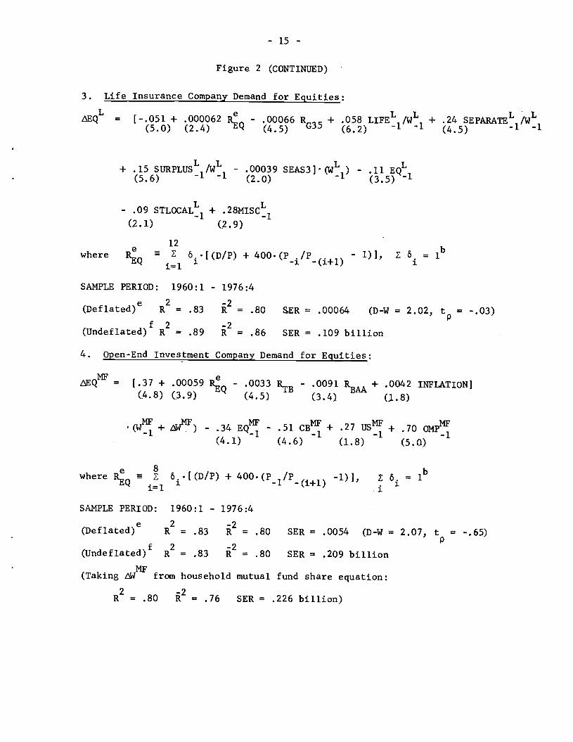
3. Life Insurance Company Demand for Equities:

QL = [051+ .000062 - .00066 R + .058 LIFEL iL + .24 SEPARATEL iwL(5.0) (2.4) Q (4.5) G35

(6.2)-1 -1 - -1

+ .15 SURPLUSL iwL - .00039 SEAS3].(wL ) - .11 EQL(5.6)

—1 —1(2.0)

—1 —1

- .09STLOCALL1 + .28MIScT1

(2.1) (2.9)

where ô..[(D/P) ÷ 400.(P./P(.+l) 1)]; 6i=

SAMPLE PERIOD: 1960:1 - 1976:4

(Deflated)e R = .83 R2 = .80 SER = .00064 (D-W = 2.02, t = -.03)

(Undeflated) R = .89 R = .86 SER = .109 billion

4. Open-End Investment Company Demand for Equities:

= [.37 + .00059 R - .0033R.B

- .0091 RB + .0042 INFLATION](4.8) (3.9) (4.5) (3.4) (1.8)

(W + iW) - .34 EQ - .51 CB + .27 US + .70 OMP(4.1) (4.6) (1.8) (5.0)

where RQ Z o..[(D/P) + 400.(P 1/P( 1)

=

SAMPLE PERIOD: 1960:1 - 1976:4

(Deflated)e R2 = .83 = .80 SER = .0054 (D-w = 2.07, t = -.65)

(iJndef1ated) R2 = .83 R2 = .80 SER = .209 billion

(Taking MF from household mutual fund share equation:

R2 = .80 2 = .76 SER = .226 billion)

- 16 -

Figure 2 (CONTINUED)

5. Private Pension Fund Demand for Equities:

QP = [.12 + .00012 R - .0020 R + .0025 INFLATION - .010 ERISA(5.2) (3.8)

G35(54)

+ .0018 SEAS4].(w' + - .13 EQ - .11 (CB + US )(2.5) —1

(5.2)—1

(4.2)—1 —1

where REQa o.[(D/P) + 400W (P ./P

(• 1)- 1)], =

SAMPLE PERIOD:8 1960:1 - 1976:4

(Deflated)e R2 = .66 2 = .60 SER = .0022 (D-w = 1.91, t = .13)

(Undef1ated) R2 = .85 2 = .83 SER = .222 billion

6. Property and Casualty Insurance Company Demand for Equities:

EQ° = .25 (SURPLUSO)e + [.44 + .00036 R - .0033 Re + .00098 INFLATION](2.4) (9.1) (5.6) (8.6) CP (2.6)

(W° + EW°) - .39 EQ - . 52 US0 - .51 STLOCAL° - .30 CB°(8.4) . (9.0) —l (9.6) 1 (57) —l

e 6 bwhere R a z ö.R , z a. = 1

CP 1=1 1 CP,-(i+l) i

e 10 b

REQa 6..[(E/P) + 100. (Ei/E(j+l) - 1, = 1

0(SURPLUSO)e Z w. .SURPLUS . , E w. =

1 -i+l . 1i=1 1

SAMPLE PERIOD: 1960:1 - 1976: 4

(Deflated)e R2 R2 = .92 SER = .0014 (D-w 1.97, t = .16)

(undef1ated) R2 = 2 = SER = .063 billion

— 17 —

Figure 2 (CONTINUED)

7. State and Local Government Retirement System Demand for Eguities:e

LEQS = [.056 + .00033 REQ - .00064 Rp - .0013 INFIATIONI.(WS1 + S)(5.5) (2.8) (2.2) (3.3)

- .097 EQS1 - .20usS1

(3.1) (4.5)

10b

where REQ Z ô..[(D/P) + 400. (P ./P(+l) 1)', = 1

i=1 3:

SANPLE PERIOD: 1966:1 - 1976:4

R2 = .73 = 68 SER = .174 billion (D-.W 1.75, t = .67)

NOTES:

aNumbers in parentheses are asymptotic t-statistics. The R2 is the coeffi-cient of determination, R2 is the coefficient of determination adjusted fordegrees of freedom, SER is the standard error of the regression, D-W isthe Durbin-Watson statistic and t is the Wald test statistic for first

porder serial correlation of the residuals. The statistic t is asymptotically

distributed as a t-statistic under the null hypothesis that the residualsdo not display serial correlation. All equations are estimated using theBrundy-Jorgenson instrumental variable technique described in the text.

bLag coefficients are constrained to lie on a third degree polynomial whichpasses through zero at the maximum lag length "i." The sum of the lagcoefficients is constrained to equal unity.

CA time dummy variable was included for 1970:3, the quarter following thePenn Central collapse.

dA time dummy variable was included for 1962:2. Households were inexplicablyvery large net sellers of equity in this quarter.

eThe sample period for this regression differs from that used in the otherregressions because of major changes that occurred in state laws governingthe investment practices of these institutions around 1966.

—18—

Figure 3

ESTIMATED EQUITY SUPPLY EQUATION FOR NON-FINANCIAL CORPORATIONSa

8. Gross Equity Issues by Domestic Non—Financial Corporations:

=-.14 ( WORKING CAPITALN)e + [.056 + .020 (P/D) + .00060 RB

(3.0) (6.3) (9.7) (6.3)

— .0000057 (R1/R)e].(DN1 + DN) — .065 SURPLUSN1 — .065 LONG DEBTN1

(3.0) (5.1) (5.1)

— .059 SHORT DEBTN1

-

(2.8)

N 6 N b( WORKING CAPITAL )e •. (woRKING CAPITAL .), E (A). = 1

i=11 —1 1

(R,R)e 400106±(Rcpi/Rcp,(i+l) — 1), ib

SAMPLE PERIOD: 1960:1 — 1976:4

R2 = .92 2 = .90 SER = .353 billion (D—W = 1.77, t .82)

NOTES:

aNbers in parentheses are asymptotic t—statistics. For other regressionsummary statistics, see note (a) of the preceding exhibit.

bLag coefficients are constrained to be on a third degree polynomial whichpasses through zero at the maximum lag length "1." The sum of the coeffi-

cients is constrained to equal unity.

—19—

Figure 4

VARIABLE DEFINITIONS

CB Holdings of corporate and foreign bonds.

D Standard and Poor's index of dividends per share.

Replacement value of capital stock of U.S. nonfinancialcorporations plus holdings of financial assets.

DN Net funds raised in financial markets plus gross equityretirements of nonfinancial corporations.

E Standard and Poor's index of earnings per share.

EQ Holdings of equities.

EEQ Net acquisitions of equities.

Nequity issues by domestic nonfinancial corpora-

tions.

ERISA Time dummy for Employee Retirement Income Security Actof 1974. Equal to 0 before and 1 from 1974:3 to1976:4.

INCOME11 Gross personal income of households (quarterly rate).

INFLATION Proxy for expected inflation. Equal to a thirteenquarter moving average of current and past rates ofinflation.

LIFEL Life insurance reserves at life insurance companies.

LIQUIDH Household holdings of liquid assets. Equal to house-hold holdings of U.S. government securities, open—market paper, time deposits and savings accounts,and money market fund shares.

LONG DEBTN Long—term debt of nonfinancial corporations.

MISCT Miscellaneous assets of life insurance companies

(primarily receivables).

—20—

Figure 4 (CONTINUED)

MFH

OMP

P

RBAA

Rcp

RG3S

1?STB

SEAS2

SEAS3

SEAS4

SEPARATEL..

SHORT DEBTN

STLOCAL

SURPLUSL

SURPLUS°

SURPLUSN

TAXDUMMY

US

w

AW

AWORKING CAPITALN

Household holdings of mutual fund shares.

Net acquisitions of mutual fund shares by households.

Holdings of open—market paper.

Standard and Poor's index of 500 common stock prices.

Moody's BAA corporate bond rate.

4—6 month prime commercial paper rate.

Market yield on 3—5 year U.S. government bonds.

Market yield on 3—month treasury bills.

Time dummy for second quarter.

Time dummy for third quarter.

Time dummy for fourth quarter.

Separate account reserves at life insurance companies.

Short—term debt of U.S. nonfinancial corporations.

Holdings of state and local government obligations.

Life insurance companies' total financial assets lesstheir total external liabilities.

Current quarter operating surplus of property andcasualty insurance companies.

Owners' equity (replacement value) in U.S. nonfinancialcorporations.

Time dummy for 1969 personal income tax revisions.Equal to 0 before 1970:1 and 1 from 1970:1 to 19.76:4.

Holdings of U.S. government securities.

Total discretionary financial wealth.

Net new inflows of discretionary financial wealth.

Change in working capital of U.S. nonfinancial

corporations.

—21—

of the mutual fund sector are held in the form of long—term corporate bonds,

15% at year—end 1976. Consequently, the long—term bond yield is in effect

one component of the total yield on new mutual fund assets. The positive

coefficient associated with the long—term bond rate in regression (1) may

reflect the fact that mutual funds are a vehicle by which investors invest

in long—term bonds.

The TAXDUMMY variable is an attempt to measure the impact on house-

holds' demands for mutual fund shares of the 1969 individual income tax

revisions. These revisions substantially increased the effective capital

gains tax rates paid by high income investors. The negative coefficient

associated with the TAXDUNMY variable suggests that this tax code change

has reduced the demand for mutual fund shares by households.

Regression (1) implies that 9.7% of the discrepancy between desired

and actual mutual fund share holdings are removed by households within a

single quarter.

Household demand for equities. The demand for directly held equities

by households is seen to be positively related to the current dividend/price

ratio and the expected rate of growth of dividends per share. This demand

is negatively related to the three month treasury bill rate and the expected

rate of return on three—five year U.S. government bonds.

The INCOME variable in the household equity eqution is the logical

counterpart to the transactions demand for money. The negative coefficient

associated with this variable in regression (2) indicates a negative trans-

actions demand for equities. Similar results have been reported by

Hendershott (1977).

—22—

A fourth quarter seasonal dummy is included in the household equity

regression in an attempt to verify the claim that. households sell off

equities in the fourth quarter for income tax reasons. In the fourth

quarter there is an incentive for individuals to reduce their taxable

income by selling securities on which they have accrued unrealized capital

losses. This incentive is higher (a) the higher were the individuals'

realized capital gains during the year and (b) the higher is the individuals'

capital gains tax rate. For these reasons, the fourth quarter seasonal

dummy is weighted by the inverse of the dividend/price ratio, to reflect

(a), and a separate seasonal dummy is included for the post 1969 tax code

revision period, to reflect (b).12

Regression 2 indicates that the fourth quarter sell—off of equities

is important and has been more pronounced in the period after the 1969 tax

code revisions. Moreover, the reported regression has a lower standard

error than an alternative regression in which the seasonal factors were

not weighted by the inverse of the dividend/price ratio. Surprisingly,

no effect of the 1969 tax code revision was discernable for the first,

second or third quarters.

Regression (2) implies that 8.5% of the discrepancy between desired

and actual household equity holdings are removed in a single quarter.

Life insurance company demand for equities. The estimated short—

run demand for equities by life insurance companies is positively related

to the expected yield on equities and negatively to the yield to maturity

on three—five year U.S. government bonds. The absence of any short—term

interest rate in this equation is not especially surprising in view of the

long—term nature of life insurance companies' liabilities.

—23—

The equity demand equation for life insurance companies includes

three institutional variables thought to play an important role in the

portfolio behavior of these institutions. These additional variables

are life insurance reserves, separate pension fund account reserves and

owners' equity as fractions of total financial assets)3

Life insurance companies' investments of life insurance reserves

are highly restricted by state regulatory authorities. In particular,

the fraction of these reserves invested in equities has been legally

restricted to well under 10% in most states throughout our sample period.

Separate pension fund account reserves, on the other hand, are virtually

unrestricted in most states. Consequently, the proportion of separate

account reserves invested in equities has tended to be quite high. From

their inception in 1967 through 1976, equities have comprised between 63%

and 86% of the value of separate account reserves. In terms of restrictions

on their use, life insurance general funds fall somewhere between life

insurance and separate account reserves.

The above considerations suggest that the composition of life insur-

ance companies' liabilities is an important influence on their portfolio

behavior. Our empirical results tend to confirm this conjecture. The

three liability variables are highly significant as explanators of life

insurance company equity demands. Moreover, the values of their coeff 1—

cients are very much in line with our prior expectations. Net acquisi-

tions of equities tend to be greatest out of separate account reserves

followed by owner's equity and life insurance reserves.

Regression (3) indicates that 11% of any undesired equity holdings

are removed by life insurance companies within a single quarter.

—24—

Open—end investment company demand for equities. The demand for

equities by this group is seen to be positively related to the own yield

on equities and negatively related to both short—term and long—term

interest rates. Increases in expected inflation appear to increase the

demand for equities by mutual funds; however, the significance of this

effect is marginal.

The estimated speed of adjustment of actual to desired equity hold-

ings is quite large, 34% per quarter. This is consistent with the well

known fact that this group of institutions has the highest equity port-

folio turnover rate of any of the major institutional investors.

Private pension fund demand for equities. This sector's short—run

demand for equities is related positively to the expected yield on equities

and negatively to the three—five year U.S. government bond rate. The

absence of any effect of short—term interest rates is not surprising given

the long term nature of this sector's liabilities. Private pension fund

equity demands also appear to be strongly affected by the expected rate

of inflation: increases in expected inflation tending to increase the

demand for equities.

The ERISA variable in regression (5) is a time dummy relfecting

congressional passage of the Employee Retirement Income Security Act of 1974.

The coefficient associated with this variable is negative and highly

significant, suggesting that the passage of this legislation has tended to

reduce the equity demands of private pension funds.

The speed of adjustment of actual to desired equity holding implied

by regression (5) is 13% per quarter.

—25—

Property and casualty insurance company demand for equities.

Regression (6) indicates that this sector's short—run equity demands are

positively related to the expected equity yield and negatively related to

the expected yield associated with rolling over short—term commercial

paper holdings Increases in expected inflation are seen to increase this

sector's equity demands.

The (SURPLUSO)e variable in regression (6) is intended to reflect

expected underwriting income. The regression implies that a $1.00

increase in expected quarterly earnings gives rise to a $.25 increase

in quarterly net acquisitions of equities.

The speed of adjustment implied by this equation is 39% per quarter.

While seemingly large, this speed of adjustment is comparable to that

reported by Friedman and Roley (1978) for this sector's corporate bond

demands.

State and local government retirement system demand for equities.

This sector's short—run demand for equities is positively related to the

expected own yield on equities and negatively related to the three—six

month commercial paper rate and expected inflation. The speed of adjust-

ment of this sector's actual to desired equity holdings is estimated to

be 9.7% per quarter.

Gross equity issues by domestic nonfinancial corporations. The

regression equation for gross equity issues by domestic nonfinancial

corporations appears in Figure 3. Gross equity issues are seen to

respond negatively to the Standard and Poor's dividend/price ratio and

positively to the level of long-term interest rates. This equation also

implies that gross equity issues fall when interest rates are expected

to rise.

—26—

It is sometimes argued that firms attempt to match the maturity

structure of their liabilities with that of their assets. That is,

firms try to finance long—term assets with long term liabilities and

short term assets with short—term liabilities. The working capital

variable in the equity supply equation is an attempt to capture this effect.

This variable is intended to represent firms' expectations about future

increases in working capital requirements. To the extent that changes

in working capital are initially considered temporary this variable should

be negatively related to current equity issues.

This prior belief is supported by regression (1) in Figure 3. In-

creases, in expected working capital requirements, holding constant the

current level of net funds raised in financial markets, tend to depress

gross equity issues.

The coefficient of lagged owner's equity in the equity supply equation

is only —.065, implying that only 6.5% of the discrepancy between the

desired and actual levels of owner's equity is removed in any given quarter

by floating new equity issues. This speed—of—adjustment is considerably

smaller than the speeds of adjustment which characterize the equity demand

equations in Figure 2. There are two possible explanations for this result.

First, owner's equity can be increased by retaining earnings as well as by

issuing new shares. The 6.5% figure cited above reflects only the pro-

pensity to raise new owner's equity by this latter route. Generally, raising

new equity by issuing new shares is viewed as more expensive in the eyes

of management than raising the funds through retained earnings. Thus,

the total proportion of the discrepancy between desired and actual

owner's equity removed in a single quarter may be substantially larger

than 6.5%.

—27—

Second, the slow speed—of—adjustment cited above may simply reflect

the higher costs associated with restructuring a firm's liabilities relative

to the costs incurred by investors in restructuring their asset portfolios.

Registration fees and other floatation costs associated with public offer-

ings of new equities normally amount to about 10% of the net proceeds,

rendering new equity issues a very expensive financing instrument. Call

provisions also normally make the refinancing of long term bond issues an

unattractive alternative.

Summary of equity demand/supply regression. On the whole, the

explanatory powers of these regressions are quite good. In terms of the

undeflated dependent variables, the R2 of these regressions vary between

.68 for state and local government retirement systems to .92 for the equity

demands of property and casualty insurance companies. The remainder of the

structural equations exhibit R2 roughly between .80 and .90.

The regression standard errors are also quite respectable, being

largest in the household equity equation. This is not surprising in view of

the fact that this sector is a residual in the flow—of—funds accounts.

Serial correlation does not appear to be a major problem in the

structural equation regressions. While the Durbin—Watson statistics are

reported for comparison purposes, the standard test based on this statistic

is not valid for the problem at hand. The t test for first order serialp

correlation described at the end of Figure 2, however, is a valid test.

In no case is this test statistic significant at the 10% level.

—28-

V. The Structural Equity Market Model

The structural model of the U.S. equity market is summarized in

Figure 5. It is made up of the eight structural equations estimated in

Section IV, ten accounting identities, a market clearing identity and

nine bridge equations. All told, there are twenty—eight equations in the

model and an equal number of endogenous variables. To facilitate the

exposition, in Figure 5 the exogenous variables are written in lower case

letters while the endogenous variables are written in upper case.

The core of the equity market model consists of equations (1) — (11).

The first eight equations are the structural demand and supply equations

estimated and discussed above. The accounting identity (9) notes the fact

that the net acquisition of financial assets by mutual funds is, by de-

finition, equal to their current surplus plus the net acquisition of mutual

fund shares by households. Household net acquisitions of mutual fund shares

are endogenously determined from equation (1). Mutual funds' current sur-

plus is approximated by the bridge equation (1) which is displayed in de-

tail in Figure 6. This surplus is highly negatively correlated with lagged

percentage changes in F, the Standard and Poor's stock price index.

The market clearing identity (11) imposes the short—run equilibrium

requirement that the market net excess flow demand for equities equals

zero. Net equity demands and supplies by sectors not explicitly modeled

• . . exog exogin Section IV (i.e., Aeq and 1eq respectively) are treated as ex—

ogenously given in this study. These exogenous flows consist of the net

acquisitions of equities by foreigners, domestic banks and security brokers

and dealers and the net equity issues in the U.S. by foreign corporations

and domestic financial corporations.14

- 29 -

Figure 5

THE U.S. EQUITY MAJIKET MODELa

(5) QP = fP[ _1 ' '-6 w1, d, rG35, inflation, erisa,

seas4, EQ1, cb"1, us1]0 0 0

(6) IEQ° = f°[P, zw , W1, e, e1, ..., e5, inflation, i surplus ,0 0 0 0 0 0i surplus1, ..., i surplus4, EQ1, stiocal cb1, us1]

(7) QS = fS[ P1, ..., P4, w5, W1, d, inflation, EQS1,

H(1) NF

(2) IEQ11

= gH[p H wH1, d, d1, ..., d4, rBM,

inflation, taxdummy, seas2, seas3, NP111, EQH1. stlocal41j

fH[ H H=w_1, d, e1, ..., e8, rTB, r35, rG3S -1'

r35,_2, rG3S 3, income, taxdummy, seas4, EQH1, NP1,

stlocal111, cb11, liquid111, PENSION111]

(3) QL = fL[ p_1,

SEPA.RATEL1,

(4) IEQMF = fMF[p ,MF MF

EQ1, cb1,

!12' W'1, d, r35, seas4, lifeL1,

SIJRPLUSL1, EQL1, stloca1T1, misc11]

WN:, d, rTB, rB, inflation,

NP NPus1, omp1]

Sus1]

(8) LEQ= hN[P, dN, dN1, d, rB, -1' .. r

N Nworking capital , working capital , ..., working

NnetworthN1, long-term debtN1, short-term debtN1]capital4,

- equity retirements

- 30 -

Figure 5 (CONTINUED)

(9) = SURPLUS +

(10) SURPLUS = q[P1, ..., P10, W, seas2, seas3, EQ1, ..., EQ2]

(11) iEQ1 + LIEQL + EQ + LEQP + EEQ° + QS + ieqexoE LEQ + eqeXOE

(12) EQH = betaH(PIP1). (EQ11+ QH)

(13) EQL = betaL (P/P1) (EQL1 + QL)

(14) EQ = beta . (PIP1) (EQ + EQ)

(15) EQ = beta (PIP1) • (EQ'+ tEQ)

(16) EQ° = beta° •(PIP1) (EQ°1 + LEQ°)

(17) EQS = beta S(PIP1) (EQ1 + QS)

(18) EQL + other assetsL

(19) EQ+ other assets

(20) EQ' + other assets

(21) a EQ° + other assets°

(22) EQS + other assetsS

(23) H aw(24) PENSIONL = alpha .

(25) SEPARATEL = gamma .

(26) SURPLUSL = - PENSIONL - 1lfL - other liabilitiesL

(27) PENSIONH a PENSIONL + + wS + pensionexog

- 31 -

Figure 5 (CONTINUED)

(28) EQH + H + PENSION + life L + other assetsH

NOTES:

a1 is important to bear in mind that the notation ,MF and EQ denotesnet acquisitions of mutual fund shares and equities respectively.These quantities differ from the changes in the actual holdings ofthese assets by the amount of unrealized capital gains accruing duringthe quarter. Changes in actual holdings can be inferred from equations(12) - (17), (19) and (23). The author regrets this confusing notation.

To facilitate reading this table all exogenous variables are written inlower case lettering while endogenous variables are written in uppercase.

- 32 -

Figure 6

a

BRIDGE EQUATION FOR E SURPLUS

SURPLUS = [-.010 + .0095 seas2 + .0090 seas3] W(8.8) (8.3) (7.8)

-1

-8

+ z 6..[(P.1/P.2 - 1) EQ2] + .47 U_ii=O

= .•o24b65

-.015

(2.i) (2.5)

= -.015 66 = -.018

(2.3) (2.6)

= -.011 87 = -.018

(1.7) (2.7)

53 = -.010 8 = -.016

(1.8) (1.4)

54 = -.012

(2.3)

SAMPLE PERIOD: 1960:1 - 1976:4

R2 = .62 = .58 SER = .174 D.W. = 1.93

NOTES:

aThe estimation method is GLS and the estimated autoregression (rho)coefficient is .47

bThe [o) are constrained to lie on a third degree polynomial.

— 33 -

Equations (12) — (28) generate the endogenous variables which when

lagged appear as arguments in (1) — (10). Relations (12) — (17) relate

the capital gains on investor groups' equity holdings to that on the

Standard and Poor's stock price index P. The exogenous weighting factors

beta are set equal to the actual historical values of the quantities

[EQ(1)/(EQ)+ EQ(1))].(P/P1) in dynamic simulations of the equity market

model. No attempt was made to explain the variation of the tibetail factors

over time because of data problems associated with the flow—of—funds equity

level series.15

The accounting identities (18) — (22) relate the total financial

asset holdings of the institutional investors to the value of their

equity and non—equity holdings. Non—equity asset holdings are treated

as exogenous in the model.

Identity (23) equates the value of households' holdings of mutual

fund shares to the value of the assets held by mutual funds.

The bridge equations (24) and (25) relate the pension and separate

account reserves of life insurance companies to the level of their total

financial assets. The simulated ratios PENSIONL/WL and SEPARATEL/WL are

constrained to equal the historical values of these quantities.

Relation (26) defines the financial surplus of life insurance

companies to be their total financial assets less the sum of pension

reserves, life insurance reserves and other liabilities.

Equation (27) is an accounting identity which stipulates that

households' pension reserves are equal to the total financial assets of

private and state and local pension funds plus the pension reserves of

life insurance companies and pension liabilities of other (exogenous)

sectors. This latter quantity consists largely of pension liabilities

of the federal government. The final equation, (28), is simply the

— 34 -

wealth identity for the household sector.

Nodel validation experiments. To assess the validity and consis-

tency of the above structural equity market model, three historical tracking

experiments are performed. Two of these are within—sample tracking tests

while the third is the out—of—sample tracking exercise.

The first validation experiment involves comparing a within—sample

(1960:1 — 1976:4) static simulation of the model's stock price variable P

with its actual historical record over the period. Simulated versus actual

values of log [P] together with the associated simulation errors

and statistics are presented in Figures 7_8)6

As can be seen from these plots, the model tracks historical stock

prices equally as well over the second half of the sample period as it does

over the first half, even though stock prices are more volatile over

the second half.

The mean simulation errors for both P and log[P1 are very small.

Their associated ENSEs are 3.2 and .040 respectively. Some serial correl-

ation is evident in the simulation residuals with the Durbin—Watson statistics

being 1.66 and 1.60 respectively.

These static simulation results compare quite favorably with those

reported by Nodigliani and Cohn. They report a RMSE of .042 and a Durbin—

Watson statistic of 1.54 for their regression of log [F] "with error

feedback."

Although our sample periods differ somewhat, the closeness of

Modigilani and Cohn's and our own static simulation RNSEs and Durbin—Watson

statistics is remarkable. This is even more striking in view of the fact that

their estimation procedure (CLS) essentially acts to minimize their within—

Figure 7

STATIC SIMULATIOI1 RESULTS FOR LOGARITH1 OF STOCK PRICE INDEXa

SYMBOL

VARIABLE

,..tual Logarithm of Stock Price Index (log[P])

x

Sim

ulat

ed L

ogarithm of Stock Price Index (log[P])

4.

-4. .4. -

4 Is

I

IS4

I

I

tO7G

I72

I7-4

Notes:

I76 t7

aSee Figure

8

for simulation statistics.

Figure 8

STATIC SIMULATION RESIDUALS FOR LOGARITHM OF STOCK PRICE INDEX

SYMBOL

VARIABLE

Simulation Residuals (log[P]

log[P])

MEAN ERROR =

0.01

5

D.W.

=

1.60

!.137

S

—Q.f37

—.1 S6

1S6-

4 166

IG6C

.1

1

1

1O7 t7

174 17

RMSE

=

0.04

0

- 37 -

sample static simulation RNSE whereas our structural estimation approach

does not directly focus on this criterion.

A more useful performance test relates to the modePs ability to

track stock prices in a fully dynamic simulation.'7 Actual and simulated

values for this exercise are presented in Figures 9-10. As these diagrams

show, the structural equity market model again tracks the historical values

of P quite well over the sample period. The mean simulation errors for P

and log[P} are small and their associate RNSEs are 4.3 and .053 respectively.

The residual plot in Figure 10 indicates substantial serial corre-

lation between successive simulation errors. The Durbin-Watson statistics

associated with the errors for P and log[P] are .76 and .74 respectively,

implying serial correlation coefficients of approximately .62 and .63 respec-

tively.

In their reduced-form regression for log[P] "without feedback,"

Modigliani and Cohn report a regression standard error of .063. This is

comparable to our own RMSE for log[P] of .053. Their estimated autoregression

coefficient of .74 in this model is also of the same order of magnitude as

our own .63. Thus, again, the structural equity market model compares quite

favorably with the Modigliani and Cohn's reduced-form model in terms of

within sample forecasting accuracy.

Modigliani and Cohn also estimate an equation for log[P] in first

differenced form. This eliminates most of their residual correlation and

yields a standard error of the regression for log[P] of .044.

In Figure 11 we have plotted the historical values of log[P] together

with those implied by the dynamic control simulation discussed above. The

simulation RNSEs for P and log[P] are 3.8 and .046 respectively while the

associated Durbin-Watson statistics are 1.92 and 1.99. Our results and

Figure 9

DY

NA

MIC

SIMULATION RESULTS FOR LOGARITHM OF STOCK PRICE INDEXa

SYMBOL

Actual Logarithm of Stock Prièe Index (log[P]) A

x S

imul

ated

Logarithm of Stock Price Index (log[P])

aSee Figure 10

for simulation statistics.

;4.2L2

.4.

1S4

1g713

VARIANCE

Notes:

1q72

1q

74

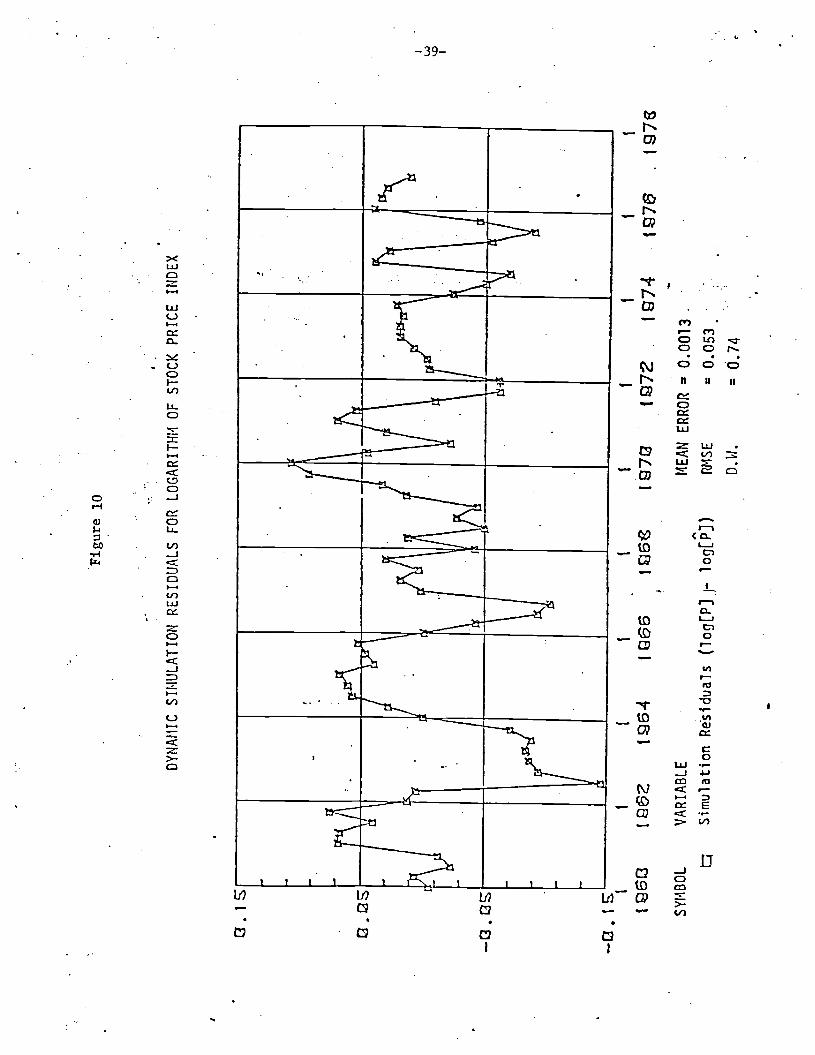
Figure 10

DYNAMIC SIMULATION RESIDUALS FOR LOGARITHM OF STOCK PRICE INDEX

17

SYMBOL t

Simulation Residuals (log[Pj— log[P])

ME

AN

E

RR

OR

0.0013

RMS E

D.W.

0.74

c.

Q.

—Q

. 16c3

1q

64

VARIABLE

U6

1g713

1q72

I7

4 17

=

0.

053

Figure 11

DYNAMIC SIMULATION RESULTS FOR

CH

AN

GE

IN LOGARITHM OF STOCK PRICE INDE(

• •j

Act

ual Change In

x

Sim

ulat

ed

Cha

nge

Loga

rithm

of

S

tock

P

rice

Inde

x (A

in Logarithm of Stock Price Index

—E3.r3

—E3.

1ss

1S6Z

SYMBOL

VARIABLE

16

I

I

1

1.

1.973

1.97

1.97-4

1976

1ogP])

(t log[P])

tIEAN E

RR

OR

0.

0024

RM

SE

=

0.

046

D.W

. 1.

99

—41—

those of Modigliani and Cohn are again in close conformity.

Our final historical tracking exercise is an out-of-sample perfor-

mance test. This experiment consists of reestimating the equity market

model using the sample period 1960:1 - 1974:4 and then simulating this

new model dynamically over the period 1975:1 - 1976:4.

The results of this exercise are presented in Figure 12. It can be

seen that the model substantially overpredicts the stock market recovery

in 1975. This, however, is not terriby surprising in light of the very

depressed level of the stock market in 1974:4.

By 1975:4 the model's stock price predictions begin to come back on

track and by 1976:1 the model is tracking stock prices very closely. In

fact, the model's predictions are extremely close to the actual values

throughout the last three quarters of 1976.

On the whole, the equity market model's out-of-sample tracking

performance seems quite respectable given the chaotic period over which

this exercise carried out. Unfortunately, Modigliani and Cohn do not

report any out-of-sample simulation experiments with their reduced-form

equity market model.

To recapitulate, we have shown that our structural model of the U.S.

equity market is highly competitive with a well known reduced-form model

of the equity market in terms of within-sample forecasting accuracy. The

structural model also performs reasonably well in an out-of-sample fore-

casting exercise. We tentatively conclude, therefore, that the available

evidence supports the use of the structural model of the determination of

the general level of equity prices.

Figu

re 1

2

OUT-OF-SAMPLE SIMULATION RESULTS FOR LOGARITHM OF STOCK PRICE INDEX

-47C3

t7

tS7

SYMBOL

VARIABLE

MEAN ERROR =

0.14

Act

ual Logarthrn of Stock Price Index (logiP])

RMSE

=

0.20

.x

Sim

ulat

ed Logarithm of Stock Price Index (log[P3)

D.W.

= 0.

31

1S77

—43--

VI. Expected Inflation and Equity Prices

Figure 13 reports the results of using the above structural equity

market model to simulate the effects on equity prices of increases in

expected inflation, nominal interest rates, and expected earnings and

dividend per share growth rates. When appropriate, comparable results

obtained by Modigliani and Cohn are also reported.

To obtain the statistics reported in Figure 13 a static control

simulation is compared to a simulation in which the indicated variables

are increased above their actual historical values by 100 basis points.

Static rather than dynamic simulations are employed to avoid having to

adjust other exogenous variables (e.g., wealth flows) to reflect the

increases in inflation that would have to occur if investors' inflation

expectations are realized)8

From Figure 13 we see that a ceterus paribus 100 basis point increase

in nominal interest rates is predicted to reduce current stock prices by

9.9%. This estimate falls well within the 957 confidence bound of the

Modigliani-Cohn estimate of 5.97g.

Holding nominal interest rates fixed, our model predicts that 100

basis point increases in expected inflation and nominal earnings and

dividends per share growth rates will raise current stock prices by l.97)

This estimate lies slightly outside the 957 confidence bound of Modigliani

and Cohn's estimate of -2.1%. Caution must be exercised in interpreting

this difference because of the fact that joint confidence bounds for both

our "estimate" and Modigliani and Cohn's are not obtainable. Hence, we cannot

determine whether or not these two predictions are statistically different.

—44—

Figure 13

MEAN CHANGE IN LOG[P] DUE TO 100 POINT INCREASE IN THE FOLLOWING VARIABLES

STRUCTURAL MODEL ESTIMATESa MODIGLIANI-COHNOF THE MEAN CHANGE IN LOG[P] ESTIMATES

1. (a) Expected inflation .015 NA

2. (b) All nominal interest rates -.099 -.059

3. (c) Expected nominal earnings .004 NAand dividends per sharegrowth rates

4. (a) and (b) -.083 NA

5. (a) and (c) .019 -.021

6. (a), (b) and (c) -.078 -.080

Notes: (a) The time interval used for these experiments is 1960:1 -1976:4. In each experiment the indicated variablesare increased 100 basis points above the actual histori-cal values used in a static control simulation. Thenumber reported above are the mean differences between

the log [PJ generated by the perturbed and by the controlsimulations.

—45—

Both Modigliani and Cohn's and our own estimate of this effect are likely

to be very imprecise due to the severe collinearity between the inflation

variables and the nominal interest rates in our respective regressions.

Given the empirical regularity that real interest rates in the U.S. have

tended to be relatively constant over time,2° both models are likely to

give better estimates of the impact of expected inflation holding real,

rather than nominal, interest rates fixed. This, moreover, is probably

the more realistic and interesting case in any event.

The predicted equity price change holding real interest rates fixed

is reported as experiment (6) and Figure 13. In this case the effect

estimated by Modigliani and Cohn (87w) is almost identical with the esti-

mate derived from the structural equity market model (7.8%). In both

models this effect is essentially due to the fact that nominal interest

rate effects on equity prices dominate handily the effects of expected

inflation per Se. Needless to say, the similarity of the above estimates

is striking given the different methodologies responsible for generating

them.

VII. Conclusions

In this paper we have constructed a structural econometric model

of the U.S. equity market and have used this model to estimate the impact

of expected inflation on the general level of equity prices. Two major

conclusions follow from this study. First, the structural equity market

model which we have constructed appears to do at least as well in several

standard within-sample historical tracking tests as the well known

Modigliani-Cohu reduced-form model. The structural model also performs

—46—

reasonably well in an out-of-sample tracking exercise. It performs well

in these model validation tests even though the estimation procedure does

not directly focus upon within-sample RNSE. The estimation procedure in

most reduced-form models, however, does directly focus on this criterion.

Second, the structural equity market model implies that increases

in expected inflation holding real interest rates fixed severely depress

stock prices. The model estimates that each 100 basis point increase in

expected inflation, holding real interest rates fixed, will reduce the

general level of equity prices by 7.87. This estimate is almost identical

to that obtained by Modigliani and Cohn who use the alternative reduced-

form methodology.

Footnotes

*1 am indebted to Benjamin Friedman and John Lintner for many helpfuldiscussions. Of course, they are not responsible for any errors whichremain.

1. For a proof see Modigliani and Cohn (1979).

2. See Jones (1979) for a discussion of how this specification is motivated.

3. Net acquisition of life insurance and pension reserves are presumed tobe contractual rather than discretionary in the short—run.

4. For most life insurance companies policy loans are nondiscretionaryinvestments.

5. Trade credit is presumed to be a nondiscretionary investment for propertyand casualty insurance companies.

6. The regression equation for this sector is not substanially affectedif instead of replacement value the market value is used.

7. Rational expectations were also tried using the approach outlined inFriedman and Roley (1977). In all cases the own yield effect isinsignificant when rational expectations are assumed. Friedman andRoley report similar findings.

8. Due to collinearity problems this expression is modeled as a distributedlag of past growth rates of earnings per share in the household equityequation.

9. New wealth flows are taken as exogenous in this study and therefore neednot be instrumented. An exception are the new wealth flows of open—endinvestment companies which are endogenously determined within the equitymarket model. These wealth flows are instrumented below. For a theoreti-cal discussion of the econometric exogeneity of new wealth flows seePurvis (1978) and Smith (1978).

10. The sample period for state and local government retirement systemsis only 1966:1 through 1976:4. See note Ce) of Figure 2 for additionaldetails.

11. See Dyl (1977) for a discussion of this effect.

12. Dyl has empirically verified these effects using monthly trading dataon individual securities.

13. As a methodological note, these three ratios are not perfectly cal—linear (i.e., they do not sum to unity) because several liabilitycategories are excluded from the regression specification. Thelargest excluded category are insured pension reserves which were 24%of total assets at the end of 1976.

14. At year—end 1976 these exogenous sectors held only 5.6% of all equity

outstanding.

15. The flow—of—funds series of end—of—quarter equity holdings are inter-polations of year—end numbers. They are therefore not very accurate.

16. Equity demands by state and local government retirement systems istreated as exogenous from 1960:1—1965:4 and is treated as fully

exogenous thereafter.

17. In a dynamic simulation the lagged endogenous variables which affectstock prices in the current period are those which were endogenouslydetermined by the model in previous periods.

18. See Nishkin (1979) for a related discussion.

19. Modigliani and Cohn implicitly assume in their regression that realearnings per share are unaffected by changes in the rate of inflation.This assumption, they maintain, is supported by the available evidence.As can be seen from Figure 13, the expected growth rates of earningsand dividends have only marginal affects on stock prices in the struc-tural equity market model anyway. Thus, our simulation experimentsare fairly insensitive to changes in the assumption of how these growthrates react to changes in inflation.

20. See the references cited by Jones (1979).