Database Management Systems 2010/11

– Chapter 7: Concurrency Control –

J. Gamper

◮ Lock-Based Protocols

◮ Graph-Based Protocols

◮ Timestamp-Based Protocols

◮ Multiple Granularity

◮ Multiversion Protocols

◮ Deadlock Handling

These slides were developed by:– Michael Bohlen, University of Zurich, Switzerland– Johann Gamper, University of Bozen-Bolzano, Italy

DMS 2010/11 J. Gamper 1/40

Lock-Based Protocols

◮ One way to ensure serializability is to require that data items be accessedin a mutually exclusive manner

◮ More precisely, while one transaction is accessing a data item, no othertransaction can modify it.

◮ Lock is the most common mechanism to implement this requirement tocontrol concurrent access to a data item.

◮ Data items can be locked in two modes:◮ exclusive mode (X): Data item can be both read as well as written. X-lock

is requested using lock-X(A) instruction.◮ shared mode (S): Data item can only be read. S-lock is requested using

lock-S(A) instruction.

◮ Locks can be released: U-lock(A)

◮ Lock requests are made to concurrency-control manager.◮ Transaction can proceed only after request is granted.

DMS 2010/11 J. Gamper 2/40

Lock-Based Protocols . . .

◮ Locking protocol: A set of rules followed by all transactions whilerequesting and releasing locks.

◮ Locking protocols restrict the set of possible schedules.

◮ Ensure serializable schedules by delaying transactions that might violateserializability.

DMS 2010/11 J. Gamper 3/40

Lock-Based Protocols . . .

◮ Lock-compatibility matrix tells whether two locks are compatible or not.◮ Any number of transactions can hold shared locks on a data item◮ If any transaction holds an exclusive lock on a data item no other

transaction may hold any lock on that item.

Lock 2S X

Lock 1 S true falseX false false

◮ Locking Rules/Protocol◮ A transaction may be granted a lock on an item if the requested lock is

compatible with locks already held on the item by other transactions.◮ If a lock cannot be granted, the requesting transaction is made to wait till

all incompatible locks held by other transactions have been released. Thelock is then granted.

DMS 2010/11 J. Gamper 4/40

Pitfalls of Lock-Based Protocols

◮ Too early unlocking can lead to non-serializable schedules.

◮ Too late unlocking can lead to deadlocks.

◮ Example:◮ Transaction T1 transfers $50 from account B to account A.◮ Transaction T2 displays the total amount of money in accounts A and B,

that is, the sum of A + B.

DMS 2010/11 J. Gamper 5/40

Pitfalls of Lock-Based Protocols . . .

◮ Example (contd.): Early unlocking cancause non-serializable schedules, andtherefore potentially incorrect results.

◮ e.g., A = $100, B = $200◮ ⇒ display A + B shows $250◮ <T1, T2> and <T2, T1> display $300

T1 T2

1. X-lock(B)2. read B3. B := B-504. write B5. U-lock(B)6. S-lock(A)7. read A8. U-lock(A)9. S-lock(B)10. read B11. U-lock(B)12. display A + B13. X-lock(A)14. read A15. A := A+5016. write A17. U-lock(A)

DMS 2010/11 J. Gamper 6/40

Pitfalls of Lock-Based Protocols . . .

◮ Example (contd.): Late unlocking can lead to deadlocks◮ Neither T1 nor T2 can make progress:

◮ executing lock-S(B) causes T2 to wait for T1 to release its lock on B.◮ executing lock-X (A) causes T1 to wait for T2 to release its lock on A.

◮ To handle a deadlock one of T1 or T2 must be rolled back and its locksreleased.

T1 T2

1. X-lock(B)2. read B3. B := B-504. write B5. S-lock(A)6. read (A)7. S-lock(B)8. X-lock(A)

DMS 2010/11 J. Gamper 7/40

Two-Phase Locking Protocol

◮ Two-Phase Locking Protocol: A locking protocol that ensuresconflict-serializable schedules. It works in two phases:

◮ Phase 1: Growing Phase

◮ transaction may obtain locks◮ transaction may not release locks

◮ Phase 2: Shrinking Phase

◮ transaction may release locks◮ transaction may not obtain locks

◮ Lock point: Transition point form phase 1 into phase 2, i.e., when the firstlock is released.

DMS 2010/11 J. Gamper 8/40

Two-Phase Locking Protocol . . .◮ Example: Schedule with locking instructions following the Two-Phase

Locking Protocol

T1 T2

1. X-lock(B)2. read B3. B := B-504. write B5. X-lock(A)6. U-lock(B)7. S-lock(B)8. read(B)9. read(A)10. A := A+5011. write(A)12. unlock(A)13. S-lock(A)14. read(A)15. display A + B16. unlock(B)17. unlock(A)

DMS 2010/11 J. Gamper 9/40

Two-Phase Locking Protocol . . .

◮ Properties of the Two-Phase Locking Protocol◮ Ensures serializability

◮ It can be shown that the transactions can be serialized in the order of theirlock points (i.e., the point where a transaction acquired its final lock).

◮ Does not ensure freedom from deadlocks◮ Cascading roll-back is possible

◮ Modifications of the two-phase locking protocol◮ Strict two-phase locking

◮ A transaction must hold all its exclusive locks till it commits/aborts◮ Avoids cascading roll-back

◮ Rigorous two-phase locking◮ All locks are held till commit/abort.◮ Transactions can be serialized in the order in which they commit.

DMS 2010/11 J. Gamper 10/40

Two-Phase Locking Protocol . . .

◮ Refinement the two-phase locking protocol with lock conversions◮ Phase 1:

◮ can acquire a lock-S on item◮ can acquire a lock-X on item◮ can convert a lock-S to a lock-X (upgrade)

◮ Phase 2:◮ can release a lock-S◮ can release a lock-X◮ can convert a lock-X to a lock-S (downgrade)

◮ Ensures serializability

◮ Strict and rigorous two-phase locking (with lock conversions) are usedextensively in DBMS.

DMS 2010/11 J. Gamper 11/40

Automatic Acquisition of Locks

◮ A transaction Ti issues the standard read/write instruction without explicitlocking calls (by the programmer).

◮ The operation read(D) is processed as follows:

if Ti has a lock on D thenread(D);

elseIf necessary wait until no other transaction has a lock-X on D;Grant Ti a lock-S on D;read(D);

end

DMS 2010/11 J. Gamper 12/40

Automatic Acquisition of Locks . . .

◮ The operation write(D) is processed as:

if Ti has a lock-X on D thenwrite(D);

elseIf necessary wait until no other transaction has any lock on D;if Ti has a lock-S on D then

Upgrade lock on D to lock-X;else

Grant Ti a lock-X on D;endwrite(D);

end

◮ All locks are released after commit or abort

DMS 2010/11 J. Gamper 13/40

Implementation of Locking

◮ A lock manager can be implemented as a separate process to whichtransactions send lock and unlock requests.

◮ The lock manager replies to a lock request by sending a lock grant message(or a message asking the transaction to roll back, in case of a deadlock).

◮ The requesting transaction waits until its request is answered.

◮ The lock manager maintains a data structure called a lock table to recordgranted locks and pending requests.

DMS 2010/11 J. Gamper 14/40

Lock-Based Protocols . . .◮ Lock table

◮ Implemented as in-memory hash tableindexed on the data item being locked

◮ Black rectangles indicate granted locks.◮ White rectangles indicate waiting

requests.◮ Records also the type of lock

granted/requested.

◮ Processing of requests:◮ New request is added to the end of the

queue of requests for the data item,and granted if it is compatible with allearlier locks.

◮ Unlock requests result in the requestbeing deleted, and later requests arechecked to see if they can now begranted.

◮ If transaction aborts, all waiting orgranted requests of the transaction aredeleted.(Index on transaction to implement thisefficiently.)

DMS 2010/11 J. Gamper 15/40

Graph-Based Protocols

◮ Graph-based protocols◮ Impose a partial order (→) on the set D = {d1, d2, ..., dh} of all data items.◮ If di → dj then any transaction accessing both di and dj must access di

before accessing dj.◮ Implies that the set D may now be viewed as a directed acyclic graph, called

a database graph.

◮ Graph-based protocols are an alternative to two-phase locking and ensureconflict serializability.

DMS 2010/11 J. Gamper 16/40

Graph-Based Protocols . . .

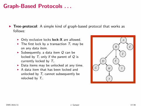
◮ Tree-protocol: A simple kind of graph-based protocol that works asfollows:

◮ Only exclusive locks lock-X are allowed.◮ The first lock by a transaction Ti may be

on any data item.◮ Subsequently, a data item Q can be

locked by Ti only if the parent of Q iscurrently locked by Ti .

◮ Data items may be unlocked at any time.◮ A data item that has been locked and

unlocked by Ti cannot subsequently berelocked by Ti .

DMS 2010/11 J. Gamper 17/40

Graph-Based Protocols . . .

◮ Example: The following 4 transactions follow the treeprotocol on thedatabase graph below.

◮ T10: lock-X(B); lock-X(E); lock-X(D); unlock(B); unlock(E); lock- X(G);unlock(D); unlock(G);

◮ T11: lock-X(D); lock-X(H); unlock(D); unlock(H);◮ T12: lock-X(B); lock-X(E); unlock(E); unlock(B);◮ T13: lock-X(D); lock-X(H); unlock(D); unlock(H);

DMS 2010/11 J. Gamper 18/40

Graph-Based Protocols . . .

◮ Example: (contd.) One possible schedule

T10 T11 T12 T13lock-X(B)

lock-X(D)lock-X(H)unlock(D)

lock-X(E)lock-X(D)unlock(B)unlock(E)

lock-X(B)lock-X(E)

unlock(H)lock-X(G)unlock(D)

lock-X(D)lock-X(H)unlock(D)unlock(H)

unlock(E)unlock(B)

unlock(G)

DMS 2010/11 J. Gamper 19/40

Graph-Based Protocols . . .

◮ The tree protocol:◮ ensures conflict serializability;◮ ensures freedom from deadlock;◮ the abort of a transaction might lead to cascading rollbacks;

◮ Unlocking may occur earlier in the tree-locking protocol than in thetwo-phase locking protocol.

◮ shorter waiting times and increase in concurrency

◮ However, in the tree-protocol a transaction may have to lock data itemsthat it does not access.

◮ increased locking overhead and additional waiting time◮ potential decrease in concurrency

◮ Schedules not possible under two-phase locking are possible under treeprotocol and vice versa.

DMS 2010/11 J. Gamper 20/40

Timestamp-Based Protocols

◮ Timestamp-based protocols◮ Each transaction gets a timestamp when it enters the system.◮ If an old transaction Ti has timestamp TS(Ti ), a new transaction Tj is

assigned timestamp TS(Tj) such that TS(Ti ) < TS(Tj).◮ The protocol manages concurrent execution such that the timestamps

determine the serializability order as follows:◮ If TS(Ti ) < TS(Tj ), the produced schedule is equivalent to the serial

schedule 〈Ti , Tj〉

◮ The protocol maintains for each data item Q two timestamp values:◮ W-timestamp(Q) is the largest time-stamp of any transaction that

executed write(Q) successfully◮ R-timestamp(Q) is the largest time-stamp of any transaction that executed

read(Q) successfully.

DMS 2010/11 J. Gamper 21/40

Timestamp-Based Protocols . . .

◮ Timestamp ordering protocol◮ Is a specific timestamp-based protocol that ensures that conflicting read

and write operations are executed in timestamp order by imposing thefollowing rules.

◮ Transaction Ti issues a read(Q):◮ If TS(Ti ) < W − timestamp(Q), then Ti needs to read a value of Q that was

already overwritten. The read operation is rejected, and Ti is rolled back.◮ If TS(Ti ) ≥ W − timestamp(Q), then the read operation is executed, and

Rtimestamp( Q) is set to the maximum of R-timestamp(Q) and TS(Ti ).

◮ Transaction Ti issues write(Q):◮ If TS(Ti ) < R − timestamp(Q), then the value of Q that Ti is producing was

needed previously, and the system assumed that that value would never beproduced. The write operation is rejected, and Ti is rolled back.

◮ If TS(Ti ) < W − timestamp(Q), then Ti is attempting to write an obsoletevalue of Q. The write operation is rejected, and Ti is rolled back.

◮ Otherwise, the write op. is executed, and W-timestamp(Q) is set to TS(Ti ).

DMS 2010/11 J. Gamper 22/40

Timestamp-Based Protocols . . .

◮ Example: The following schedule is possible under the timestamp orderingprotocol.

◮ Since we assume TS(T14) < TS(T15), the schedule must be conflictequivalent to the schedule 〈T14, T15〉

T14 T15

read(B)read(B)B := B - 50write(B)

read(A)read(A)

display(A+B)A := A + 50write(A)display(A+B)

DMS 2010/11 J. Gamper 23/40

Timestamp-Based Protocols . . .

◮ Properties of the timestamp-ordering protocol◮ Guarantees conflict serializability, since conflicting operations are processed

in timestamp order.◮ All arcs in the precedence graph are of the following form

◮ Thus, there will be no cycles in the precedence graph

◮ Ensures freedom from deadlock as no transaction ever waits.◮ The schedule may not be cascade-free and may not even be recoverable.

DMS 2010/11 J. Gamper 24/40

Timestamp-Based Protocols . . .

◮ Recoverability and cascade freedom in the timestamp-ordering protocol◮ Suppose Ti aborts, but Tj has read a data item written by Ti

◮ Then Tj must abort; if Tj had been allowed to commit earlier, the scheduleis not recoverable.

◮ Further, any transaction that has read a data item written by Tj must abort,which might lead to a cascading rollback.

◮ Solution:◮ All writes are performed at the end of a transaction and they form an

atomic action in the sense that while the writes are in progress notransaction may access any of the data items that have been written.

◮ A transaction that aborts is restarted with a new timestamp.

DMS 2010/11 J. Gamper 25/40

Multiple Granularity

◮ Instead of locks on individual data items, sometimes it is advantageous togroup several data items and to treat them as one individualsynchronization unit (e.g. if a transaction accesses the entire DB).

◮ Define a hierarchy of data granularities of different size, where the smallgranularities are nested within larger ones.

◮ Can be represented graphically as a tree

◮ When a transaction locks a node in the tree explicitly, it implicitly locks allthe node’s descendents in the same mode.

DMS 2010/11 J. Gamper 26/40

Multiple Granularity . . .

◮ Example: Graphical representation of a hierarchy of granularities◮ The highest level is the entire database.◮ The levels below are of type area, file and record in that order.

◮ Granularity of locking (= level in tree where locking is done):◮ fine granularity (lower in tree): high concurrency, high locking overhead◮ coarse granularity (higher in tree): low locking overhead, low concurrency

DMS 2010/11 J. Gamper 27/40

Multiversion Protocols

◮ Concurrency control protocols studied thus far ensure serializability byeither delaying an operation or aborting the transaction.

◮ Multiversion protocols keep old versions of data items to increaseconcurrency.

◮ Each successful write(Q) creates a new version of Q.◮ Timestamps are used to label versions.

◮ When a read(Q) operation is issued, select an appropriate version of Qbased on the timestamp of the transaction.

◮ Reads never have to wait as an appropriate version is available.

◮ Two types of multiversion protocols◮ Multiversion timestamp ordering◮ Multiversion two-phase locking

DMS 2010/11 J. Gamper 28/40

Multiversion Timestamp Ordering

◮ Multiversion timestamp ordering protocol◮ For each data item Q a sequence of versions 〈Q1, Q2, ...., Qm〉 is maintained.◮ Each version Qk contains 3 data fields:

◮ Content – value of version Qk .◮ W-timestamp(Qk ) – timestamp of the transaction that created (wrote)

version Qk◮ R-timestamp(Qk ) – largest timestamp of transaction that successfully read

version Qk

◮ When a transaction Ti creates a new version Qk of Q, the W-timestampand R-timestamp of Qk are initialized to TS(Ti ).

◮ R-timestamp of Qk is updated whenever a transaction Tj reads Qk , andTS(Tj) > R-timestamp(Qk).

DMS 2010/11 J. Gamper 29/40

Multiversion Timestamp Ordering . . .

◮ The following multiversion timestamp-ordering protocol ensuresserializability.

1. If transaction Ti issues a read(Q), then the value returned is the content ofversion Qk , which is the version of Q with the largest write timestamp lessthan or equal to TS(Ti )

2. If transaction Ti issues a write(Q):◮ If TS(Ti ) < R-timestamp(Qk), then transaction Ti is rolled back◮ Otherwise, if TS(Ti ) = W-timestamp(Qk), the contents of Qk are

overwritten.◮ Otherwise a new version of Q is created.

DMS 2010/11 J. Gamper 30/40

Multiversion Timestamp Ordering . . .

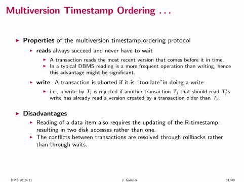
◮ Properties of the multiversion timestamp-ordering protocol

◮ reads always succeed and never have to wait

◮ A transaction reads the most recent version that comes before it in time.◮ In a typical DBMS reading is a more frequent operation than writing, hence

this advantage might be significant.

◮ write: A transaction is aborted if it is “too late”in doing a write

◮ i.e., a write by Ti is rejected if another transaction Tj that should read T ′

i s

write has already read a version created by a transaction older than Ti .

◮ Disadvantages◮ Reading of a data item also requires the updating of the R-timestamp,

resulting in two disk accesses rather than one.◮ The conflicts between transactions are resolved through rollbacks rather

than through waits.

DMS 2010/11 J. Gamper 31/40

Deadlock Handling

◮ Consider the following two transactions:

T1: write (X) T2: write(Y)write(Y) write(X)

◮ Schedule with a deadlock

T1 T2

lock-X on Xwrite (X)

lock-X on Ywrite (Y)wait for lock-X on X

wait for lock-X on Y

DMS 2010/11 J. Gamper 32/40

Deadlock Handling . . .

◮ Deadlock: A system is in a deadlock state if there is a set of transactionssuch that every transaction in the set is waiting for another transaction inthe set.

◮ A deadlock has to be resolved by rolling back some of the transactionsinvolved in the deadlock.

◮ Deadlocks are addressed in two ways:◮ Deadlock prevention protocols are used◮ Deadlocks are detected and resolved

DMS 2010/11 J. Gamper 33/40

Deadlock Prevention Protocols

◮ Deadlock prevention protocols ensure that the system will never enterinto a deadlock state.

◮ Some prevention strategies:◮ Require that each transaction locks all its data items before it begins

execution (pre-declaration).◮ Difficult to know in advance◮ Data-item utilization may be very low

◮ Impose partial ordering of all data items and require that a transaction canlock data items only in the order specified by the partial order (graph-basedprotocol).

◮ Tree protocol◮ Data items have to be known in advance

DMS 2010/11 J. Gamper 34/40

Deadlock Prevention Protocols . . .

◮ Deadlock prevention protocols using transaction timestamps.◮ Wait-die scheme◮ Wound-wait scheme

◮ Wait-die scheme - non-preemptive technique◮ Older transaction may wait for younger one to release data item. Younger

transactions never wait for older ones; they are rolled back instead (dies)

◮ Example: Transactions T22,T23,T24 with timestamps 5, 10, 15◮ T22 requests data item held by T23 : T22 will wait◮ T24 requests data item held by T23 : T24 will be rolled back.

◮ A transaction may die several times before acquiring the needed data item

DMS 2010/11 J. Gamper 35/40

Deadlock Prevention Protocols . . .

◮ Wound-wait scheme - preemptive technique◮ Older transaction wounds (forces rollback) of younger transaction instead of

waiting for it. Younger transactions may wait for older ones

◮ Example: Transactions T22,T23,T24 with timestamps 5, 10, 15◮ T22 requests data item held by T23 : T23 will be rolled back◮ T24 requests data item held by T23 : T24 will wait.

◮ May be fewer rollbacks than wait-die scheme.

◮ Both in wait-die and in wound-wait protocols, a rolled-back transaction isrestarted with its original timestamp. Older transactions thus haveprecedence over newer ones, and starvation is hence avoided.

DMS 2010/11 J. Gamper 36/40

Deadlock Prevention Protocols . . .

◮ Timeout-based protocols◮ A transaction waits for a lock only for a specified amount of time. After

that, the wait times out and the transaction is rolled back.◮ Thus, deadlocks are not possible.◮ Simple to implement; but starvation is possible. Also difficult to determine

good value of the timeout interval.

DMS 2010/11 J. Gamper 37/40

Deadlock Detection and Recovery

◮ Deadlocks can be described as a wait-for graph, which consists of a pairG = (V ,E )

◮ V is a set of vertices representing all the transactions◮ E is a set of edges; each element is an ordered pair Ti → Tj .

◮ If Ti → Tj is in E, there is a directed edge from Ti to Tj , implying that Ti

is waiting for Tj to release a data item.

◮ If Ti requests a data item being held by Tj , edge Ti → Tj is inserted in thewait-for graph. This edge is removed when Tj is no longer holding a dataitem needed by Ti .

◮ The system is in a deadlock state if and only if the wait-for graph has acycle.

◮ A deadlock-detection algorithm must be invoked periodically to look forcycles.

DMS 2010/11 J. Gamper 38/40

Deadlock Detection and Recovery . . .

◮ Wait-for graph without a cycle ◮ Wait-for graph with a cycle

DMS 2010/11 J. Gamper 39/40

Deadlock Detection and Recovery . . .

◮ When a deadlock is detected, the system must recover from the deadlock.

◮ The most common solution is to roll back one or more transactions tobreak the deadlock. Three actions are required:

1. Selection of a victim: Select that transaction(s) to roll back that will incurminimum cost.

2. Rollback: Determine how far to roll back transaction◮ Total rollback: Abort the transaction and then restart it.◮ More effective to roll back transaction only as far as necessary to break

deadlock.

3. Check Starvation: happens if same transaction is always chosen as victim.

◮ Include the number of rollbacks in the cost factor to avoid starvation

DMS 2010/11 J. Gamper 40/40