
Cost Models for Overlapping and Multiversion Structuresdimitris/PAPERS/TODS02-CM.pdf · Cost Models...
44
Cost Models for Overlapping and Multiversion Structures YUFEI TAO Hong Kong University of Science and Technology DIMITRIS PAPADIAS Hong Kong University of Science and Technology and JUN ZHANG Hong Kong University of Science and Technology Overlapping and multiversion techniques are two popular frameworks that transform an ephemeral index into a multiple logical-tree structure in order to support versioning databases. Although both frameworks have produced numerous efficient indexing methods, their performance analysis is rather limited; as a result there is no clear understanding about the behavior of the alternative structures and the choice of the best one, given the data and query characteristics. Furthermore, query optimization based on these methods is currently impossible. These are serious problems due to the incorporation of overlapping and multiversion techniques in several traditional (e.g., financial) and emerging (e.g., spatiotemporal) applications. In this article, we reduce performance analysis of overlapping and multiversion structures to that of the corresponding ephemeral struc- tures, thus simplifying the problem significantly. This reduction leads to accurate cost models that predict the sizes of the trees, the node/page accesses, and selectivity of queries. Furthermore, the models offer significant insight into the behavior of the structures and provide guidelines about the selection of the most appropriate method in practice. Extensive experimentation proves that the proposed models yield errors below 5 and 15% for uniform and nonuniform data, respectively. Categories and Subject Descriptors: H.3.1 [Information Storage and Retrieval]: Content Analysis and Indexing—indexing methods General Terms: Theory Additional Key Words and Phrases: Database, temporal, spatiotemporal, index, overlapping and multiversion structures 1. INTRODUCTION Supporting objects whose attributes change with time (i.e., versioning objects) is crucial for a large number of applications. As an example, consider a banking This work was supported by grants HKUST 6081/01E and 6197/02E from Hong Kong RGC. Authors’ addresses: Y. Tao, Department of Computer Science, Hong Kong University of Science and Technology, Clear Water Bay, Hong Kong; email: [email protected]; D. Papadias, Department of Computer Science, Hong Kong University of Science and Technology, Clear Water Bay, Hong Kong; email: [email protected]; J. Zhang, Department of Computer Science, Hong Kong University of Science and Technology, Clear Water Bay, Hong Kong; email: [email protected]. Permission to make digital/hard copy of part or all of this work for personal or classroom use is granted without fee provided that the copies are not made or distributed for profit or commercial advantage, the copyright notice, the title of the publication, and its date appear, and notice is given that copying is by permission of the ACM, Inc. To copy otherwise, to republish, to post on servers, or to redistribute to lists, requires prior specific permission and/or a fee. C 2002 ACM 0362-5915/02/0900-0299 $5.00 ACM Transactions on Database Systems, Vol. 27, No. 3, September 2002, Pages 299–342.
Transcript of Cost Models for Overlapping and Multiversion Structuresdimitris/PAPERS/TODS02-CM.pdf · Cost Models...
Cost Models for Overlapping andMultiversion Structures
YUFEI TAOHong Kong University of Science and TechnologyDIMITRIS PAPADIASHong Kong University of Science and TechnologyandJUN ZHANGHong Kong University of Science and Technology
Overlapping and multiversion techniques are two popular frameworks that transform an ephemeralindex into a multiple logical-tree structure in order to support versioning databases. Although bothframeworks have produced numerous efficient indexing methods, their performance analysis israther limited; as a result there is no clear understanding about the behavior of the alternativestructures and the choice of the best one, given the data and query characteristics. Furthermore,query optimization based on these methods is currently impossible. These are serious problemsdue to the incorporation of overlapping and multiversion techniques in several traditional (e.g.,financial) and emerging (e.g., spatiotemporal) applications. In this article, we reduce performanceanalysis of overlapping and multiversion structures to that of the corresponding ephemeral struc-tures, thus simplifying the problem significantly. This reduction leads to accurate cost models thatpredict the sizes of the trees, the node/page accesses, and selectivity of queries. Furthermore, themodels offer significant insight into the behavior of the structures and provide guidelines aboutthe selection of the most appropriate method in practice. Extensive experimentation proves thatthe proposed models yield errors below 5 and 15% for uniform and nonuniform data, respectively.
Categories and Subject Descriptors: H.3.1 [Information Storage and Retrieval]: ContentAnalysis and Indexing—indexing methods
General Terms: Theory
Additional Key Words and Phrases: Database, temporal, spatiotemporal, index, overlapping andmultiversion structures
1. INTRODUCTION
Supporting objects whose attributes change with time (i.e., versioning objects)is crucial for a large number of applications. As an example, consider a banking
This work was supported by grants HKUST 6081/01E and 6197/02E from Hong Kong RGC.Authors’ addresses: Y. Tao, Department of Computer Science, Hong Kong University of Scienceand Technology, Clear Water Bay, Hong Kong; email: [email protected]; D. Papadias, Department ofComputer Science, Hong Kong University of Science and Technology, Clear Water Bay, Hong Kong;email: [email protected]; J. Zhang, Department of Computer Science, Hong Kong University ofScience and Technology, Clear Water Bay, Hong Kong; email: [email protected] to make digital/hard copy of part or all of this work for personal or classroom use isgranted without fee provided that the copies are not made or distributed for profit or commercialadvantage, the copyright notice, the title of the publication, and its date appear, and notice is giventhat copying is by permission of the ACM, Inc. To copy otherwise, to republish, to post on servers,or to redistribute to lists, requires prior specific permission and/or a fee.C© 2002 ACM 0362-5915/02/0900-0299 $5.00
ACM Transactions on Database Systems, Vol. 27, No. 3, September 2002, Pages 299–342.
300 • Y. TAO et al.
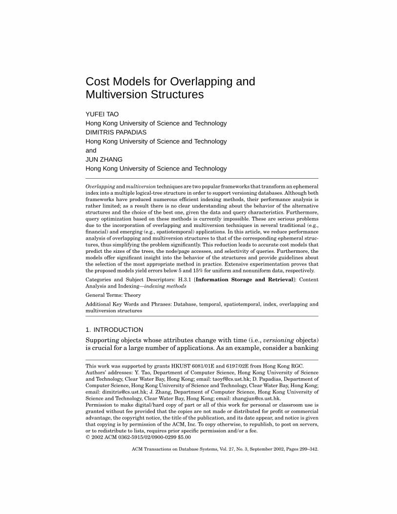
Fig. 1. Representation of versioning objects.
system that records the historical changes of account balances occurring as aresult of withdrawals, deposits, or money transfers. Old versions of the recordsare not removed since possible queries may occur regarding any time in history,and the DBMS should provide efficient access paths to all recorded versions.Such versioning databases constitute the core of many temporal, spatiotempo-ral, decision-making, and online analytical systems.
We use the term features to refer to the time-varying attributes of version-ing objects, which are best modeled as intervals in the feature–time space.Figure 1 shows an example for a banking system. The vertical axis refersto account balances (i.e., the features), and the horizontal axis correspondsto transaction time. Intervals a1, a2, and a3 represent the balance changesof account a: one withdrawal at timestamp t1 and one deposit at times-tamp t2. No change occurs to account b during the demonstrated period. No-tice that we represent records as semiclosed intervals to emphasize that thevalid period of a record does not include the last timestamp, when a newrecord becomes valid. In the sequel, we say that a record is alive during itsvalid period, and dead outside it. For example, record a2 is alive in interval[t1, t2).
An important type of processing in versioning databases involves range-interval queries (interval queries, for short), which consist of two predicates:the time interval of interest and a feature range in the feature universe. Forthe previous example, the feature universe is the range defined by the min-imum and maximum possible balances. As another scenario consider trafficcontrol systems that monitor and record movements of vehicles. In this case,the feature universe is a 2-D region that involves all the locations to whichany vehicle can ever travel. The records retrieved by a query must be aliveduring the time interval and have their features in the feature range. In-stances of range-interval queries are: “Find the accounts with balances greaterthan $1000 during March 2001,” and “Which cars appeared in the campusyesterday 8 am to 6 pm?” When the time predicate involves only a singletimestamp, the query is called a range-timestamp query (timestamp query, forshort).
Access methods for versioning databases have been extensively studied intemporal and spatiotemporal databases. Most existing methods are based onmultiple logical-tree structures (MLTS). A MLTS maintains several logical trees,each of which is an ephemeral structure suitable for indexing objects at a
ACM Transactions on Database Systems, Vol. 27, No. 3, September 2002.
Overlapping and Multiversion Structures • 301
single timestamp. To avoid excessive space storage, consecutive logical treesmay share common branches so that these branches are stored only once. Theoverlapping and multiversion techniques are two popular frameworks for con-verting ephemeral structures (such as B-trees, R-trees [Guttman 1984], linearquadtrees [Gargantini 1982], etc.) into efficient temporal and spatiotemporalaccess methods.
Despite the large number of MLTS that have been proposed, little work hasbeen carried out on their performance analysis. Existing models mainly focuson the overlapping and multiversion B-trees, merely discussing their asymp-totic optimality with respect to timestamp queries. This is, however, insuffi-cient for practical use for several reasons. First, in most cases asymptotic per-formance does not accurately reflect the actual cost. Second, interval queries,which are more frequent in practice, are not discussed. Third, existing analysisis only applicable to structures based on B-trees and cannot be used for otherMLTS.
In this article, we provide an analytical framework that can be employedfor any MLTS provided there exists a cost model for the correspondingephemeral structure. For instance, in order to analyze the performance ofMLTS based on R-trees, we only need to incorporate the corresponding R-tree models into our framework. The proposed models can accurately predict(1) tree sizes, (2) timestamp and interval query performance, and (3) queryselectivity. The formulae are based only on the properties of the raw dataand the underlying file system, and hence do not require knowledge aboutthe structures of the trees. Furthermore, they are applicable for any datadistribution and variable agility, and can be used in the presence of LRUbuffers. Our analysis can be employed to tune the structural parameters inorder to optimize the performance. Moreover, it provides significant insightinto the behavior of alternative structures, and leads to important guidelinesabout the selection of the most appropriate method given the data and querycharacteristics.
We deal with partially persistent trees [Salzberg and Tsotras 1999] (i.e., up-dates can be applied at the current timestamp only), not including structures(e.g., Lanka and Mays [1991]) where updates are allowed at any timestampin history. Furthermore, to facilitate analysis we make the following assump-tions: every object has the same probability to issue a change at each times-tamp; and the number of insertions approximates the number of deletions ateach timestamp. Note that these conditions are satisfied in a wide range ofapplications (e.g., systems dealing with bank accounts, university transcripts,employee records, vehicle movements, multimedia objects, etc.). The rest of thearticle is organized as follows. Section 2 surveys overlapping and multiversionstructures and describes in detail the two frameworks using B-trees as theephemeral structures. Section 3 presents the cost models for methods based onB-trees, and Section 4 discusses their extensions to support general structuresin real-life scenarios (LRU buffers and arbitrary data distributions). Section 5presents an extensive experimental evaluation, and Section 6 concludes thearticle with future directions.
ACM Transactions on Database Systems, Vol. 27, No. 3, September 2002.
302 • Y. TAO et al.
2. OVERLAPPING AND MULTIVERSION ACCESS METHODS
The overlapping technique was introduced in Burton and Huntbach [1985] andCarey et al. [1986] to produce a time and space efficient approach to file shar-ing. The idea was applied to B-trees in Burton et al. [1990] and R-trees inXu et al. [1990] and Nascimento and Silva [1998]. The resulting structureswere called overlapping B-trees (OVB-trees) and historical R-trees (HR-trees),respectively. Tzouramanis et al. [1999] extended OVB-trees by integratingpointers among leaf pages, which improved the so-called key-history queriesin temporal databases. The technique was also applied to linear quadtrees[Tzouramanis et al. 2000a] and spatiotemporal data warehousing [Papadiaset al. 2002]. In a survey paper Salzberg and Tsotras [1999] compared asymp-totic performance of overlapping structures with other temporal access methodsin terms of timestamp query performance, update costs, and structure sizes. In-terval query performance was not discussed.
The earliest multiversion structure appeared in Easton [1986], who proposedthe write-once B-tree (WOB-tree) for write-once-read-many (WORM) disks. Fo-cusing on a combination of WORM (for historical data) and write-many-read-many (WMRM, for current data) disks, Lomet and Salzberg [1989] presentedthe time-split B-tree (TSB-tree), which, as analyzed in Lomet and Salzberg[1990], introduced less redundancy than WOB-trees, and thus reduced the in-dex size considerably. Becker et al. [1996] optimized the multiversion frame-work (in terms of asymptotical performance for space and timestamp query cost)in their multiversion B-tree (MVB-tree), which is similar to the TSB-tree, butemploys an important mechanism called the version condition (to be elaboratedupon shortly). Varman and Verma [1997] discussed a variation of MVB-treesthat reduced the size requirements by some constant factor.
Multiversion structures based on R-trees include BTR-trees to index bitem-poral databases [Kumar et al. 1998], PPR-trees [Kollios et al. 2001], and MV3R-trees [Tao and Papadias 2001a] for spatiotemporal databases. Multiversionlinear quadtrees were proposed for image processing in Tzouramanis et al.[2000b]. The concept was also applied in branched temporal databases [Jianget al. 2000] and temporal aggregation [Zhang et al. 2001], respectively, to ob-tain BT-trees and multiversion SB-trees. Recently, Chien et al. [2002] adoptedthe technique for XML processing, and Tao et al. [2002] used it for aggregateprocessing of planar points. Despite the large number of structures, to the bestof our knowledge there does not exist any work that estimates the sizes andperformance of multiversion methods in terms of node accesses for intervalqueries.
In the rest of the section, we describe the overlapping and multiversionframeworks using B-trees as the ephemeral structure. Other MLTS can be con-structed by applying the same transformation algorithms on the correspondingephemeral structures.
2.1 Overlapping B-Trees
The idea behind OVB-trees is to maintain a separate B-tree for each times-tamp in history, but allow consecutive trees to share branches as long as the
ACM Transactions on Database Systems, Vol. 27, No. 3, September 2002.
Overlapping and Multiversion Structures • 303
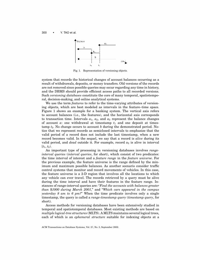
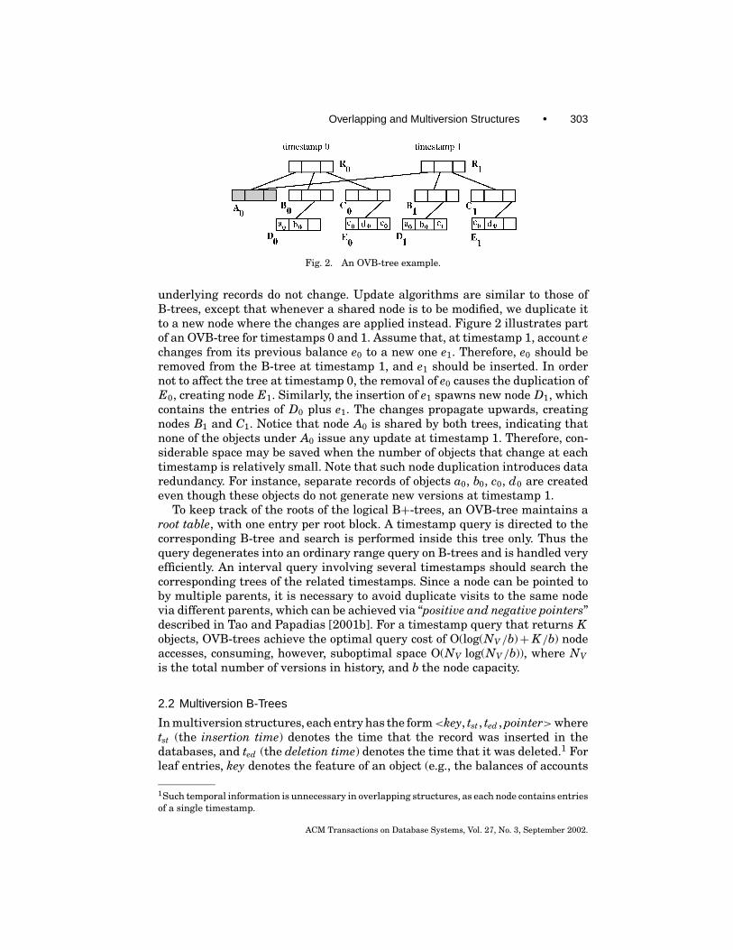
Fig. 2. An OVB-tree example.
underlying records do not change. Update algorithms are similar to those ofB-trees, except that whenever a shared node is to be modified, we duplicate itto a new node where the changes are applied instead. Figure 2 illustrates partof an OVB-tree for timestamps 0 and 1. Assume that, at timestamp 1, account echanges from its previous balance e0 to a new one e1. Therefore, e0 should beremoved from the B-tree at timestamp 1, and e1 should be inserted. In ordernot to affect the tree at timestamp 0, the removal of e0 causes the duplication ofE0, creating node E1. Similarly, the insertion of e1 spawns new node D1, whichcontains the entries of D0 plus e1. The changes propagate upwards, creatingnodes B1 and C1. Notice that node A0 is shared by both trees, indicating thatnone of the objects under A0 issue any update at timestamp 1. Therefore, con-siderable space may be saved when the number of objects that change at eachtimestamp is relatively small. Note that such node duplication introduces dataredundancy. For instance, separate records of objects a0, b0, c0, d0 are createdeven though these objects do not generate new versions at timestamp 1.
To keep track of the roots of the logical B+-trees, an OVB-tree maintains aroot table, with one entry per root block. A timestamp query is directed to thecorresponding B-tree and search is performed inside this tree only. Thus thequery degenerates into an ordinary range query on B-trees and is handled veryefficiently. An interval query involving several timestamps should search thecorresponding trees of the related timestamps. Since a node can be pointed toby multiple parents, it is necessary to avoid duplicate visits to the same nodevia different parents, which can be achieved via “positive and negative pointers”described in Tao and Papadias [2001b]. For a timestamp query that returns Kobjects, OVB-trees achieve the optimal query cost of O(log(NV /b)+ K /b) nodeaccesses, consuming, however, suboptimal space O(NV log(NV /b)), where NVis the total number of versions in history, and b the node capacity.
2.2 Multiversion B-Trees
In multiversion structures, each entry has the form<key, tst , ted , pointer>wheretst (the insertion time) denotes the time that the record was inserted in thedatabases, and ted (the deletion time) denotes the time that it was deleted.1 Forleaf entries, key denotes the feature of an object (e.g., the balances of accounts
1Such temporal information is unnecessary in overlapping structures, as each node contains entriesof a single timestamp.
ACM Transactions on Database Systems, Vol. 27, No. 3, September 2002.
304 • Y. TAO et al.
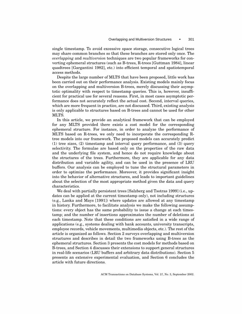
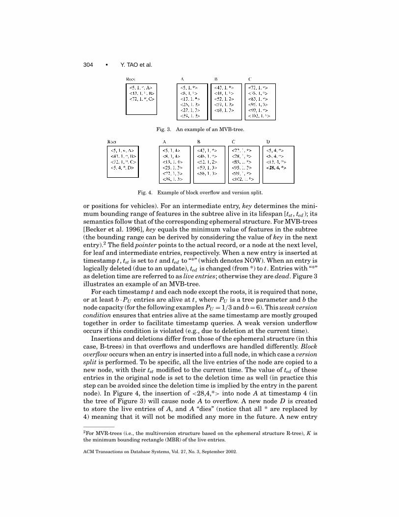
Fig. 3. An example of an MVB-tree.
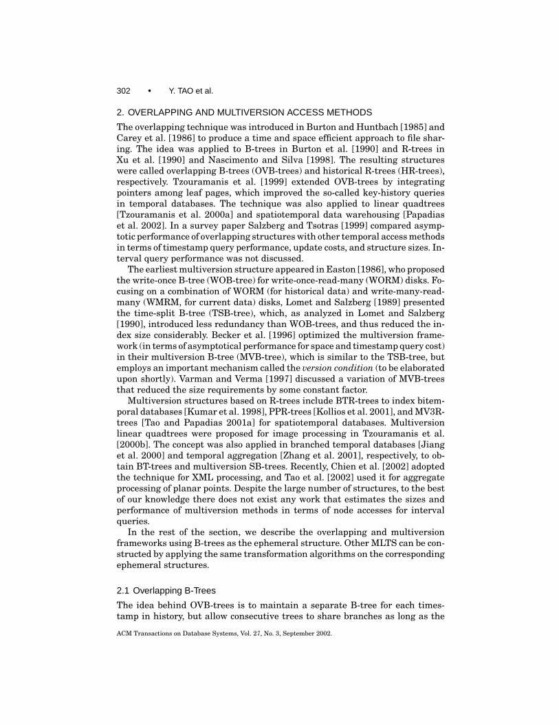
Fig. 4. Example of block overflow and version split.
or positions for vehicles). For an intermediate entry, key determines the mini-mum bounding range of features in the subtree alive in its lifespan [tst , ted ); itssemantics follow that of the corresponding ephemeral structure. For MVB-trees[Becker et al. 1996], key equals the minimum value of features in the subtree(the bounding range can be derived by considering the value of key in the nextentry).2 The field pointer points to the actual record, or a node at the next level,for leaf and intermediate entries, respectively. When a new entry is inserted attimestamp t, tst is set to t and ted to “*” (which denotes NOW). When an entry islogically deleted (due to an update), ted is changed (from *) to t. Entries with “*”as deletion time are referred to as live entries; otherwise they are dead. Figure 3illustrates an example of an MVB-tree.
For each timestamp t and each node except the roots, it is required that none,or at least b ·PU entries are alive at t, where PU is a tree parameter and b thenode capacity (for the following examples PU = 1/3 and b= 6). This weak versioncondition ensures that entries alive at the same timestamp are mostly groupedtogether in order to facilitate timestamp queries. A weak version underflowoccurs if this condition is violated (e.g., due to deletion at the current time).
Insertions and deletions differ from those of the ephemeral structure (in thiscase, B-trees) in that overflows and underflows are handled differently. Blockoverflow occurs when an entry is inserted into a full node, in which case a versionsplit is performed. To be specific, all the live entries of the node are copied to anew node, with their tst modified to the current time. The value of ted of theseentries in the original node is set to the deletion time as well (in practice thisstep can be avoided since the deletion time is implied by the entry in the parentnode). In Figure 4, the insertion of <28,4,*> into node A at timestamp 4 (inthe tree of Figure 3) will cause node A to overflow. A new node D is createdto store the live entries of A, and A “dies” (notice that all * are replaced by4) meaning that it will not be modified any more in the future. A new entry
2For MVR-trees (i.e., the multiversion structure based on the ephemeral structure R-tree), K isthe minimum bounding rectangle (MBR) of the live entries.
ACM Transactions on Database Systems, Vol. 27, No. 3, September 2002.
Overlapping and Multiversion Structures • 305
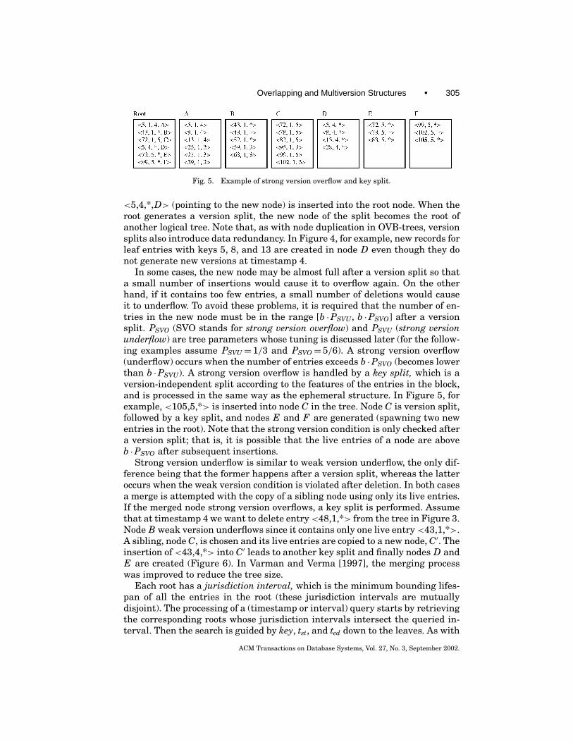
Fig. 5. Example of strong version overflow and key split.
<5,4,*,D> (pointing to the new node) is inserted into the root node. When theroot generates a version split, the new node of the split becomes the root ofanother logical tree. Note that, as with node duplication in OVB-trees, versionsplits also introduce data redundancy. In Figure 4, for example, new records forleaf entries with keys 5, 8, and 13 are created in node D even though they donot generate new versions at timestamp 4.
In some cases, the new node may be almost full after a version split so thata small number of insertions would cause it to overflow again. On the otherhand, if it contains too few entries, a small number of deletions would causeit to underflow. To avoid these problems, it is required that the number of en-tries in the new node must be in the range [b ·PSVU, b ·PSVO] after a versionsplit. PSVO (SVO stands for strong version overflow) and PSVU (strong versionunderflow) are tree parameters whose tuning is discussed later (for the follow-ing examples assume PSVU= 1/3 and PSVO= 5/6). A strong version overflow(underflow) occurs when the number of entries exceeds b ·PSVO (becomes lowerthan b ·PSVU). A strong version overflow is handled by a key split, which is aversion-independent split according to the features of the entries in the block,and is processed in the same way as the ephemeral structure. In Figure 5, forexample, <105,5,*> is inserted into node C in the tree. Node C is version split,followed by a key split, and nodes E and F are generated (spawning two newentries in the root). Note that the strong version condition is only checked aftera version split; that is, it is possible that the live entries of a node are aboveb ·PSVO after subsequent insertions.
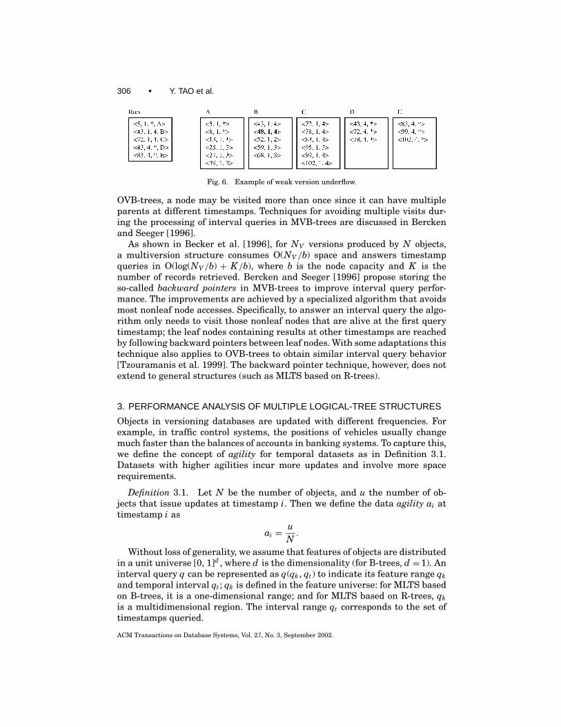
Strong version underflow is similar to weak version underflow, the only dif-ference being that the former happens after a version split, whereas the latteroccurs when the weak version condition is violated after deletion. In both casesa merge is attempted with the copy of a sibling node using only its live entries.If the merged node strong version overflows, a key split is performed. Assumethat at timestamp 4 we want to delete entry<48,1,*> from the tree in Figure 3.Node B weak version underflows since it contains only one live entry<43,1,*>.A sibling, node C, is chosen and its live entries are copied to a new node, C′. Theinsertion of <43,4,*> into C′ leads to another key split and finally nodes D andE are created (Figure 6). In Varman and Verma [1997], the merging processwas improved to reduce the tree size.
Each root has a jurisdiction interval, which is the minimum bounding lifes-pan of all the entries in the root (these jurisdiction intervals are mutuallydisjoint). The processing of a (timestamp or interval) query starts by retrievingthe corresponding roots whose jurisdiction intervals intersect the queried in-terval. Then the search is guided by key, tst, and ted down to the leaves. As with
ACM Transactions on Database Systems, Vol. 27, No. 3, September 2002.
306 • Y. TAO et al.
Fig. 6. Example of weak version underflow.
OVB-trees, a node may be visited more than once since it can have multipleparents at different timestamps. Techniques for avoiding multiple visits dur-ing the processing of interval queries in MVB-trees are discussed in Berckenand Seeger [1996].
As shown in Becker et al. [1996], for NV versions produced by N objects,a multiversion structure consumes O(NV /b) space and answers timestampqueries in O(log(NV /b) + K /b), where b is the node capacity and K is thenumber of records retrieved. Bercken and Seeger [1996] propose storing theso-called backward pointers in MVB-trees to improve interval query perfor-mance. The improvements are achieved by a specialized algorithm that avoidsmost nonleaf node accesses. Specifically, to answer an interval query the algo-rithm only needs to visit those nonleaf nodes that are alive at the first querytimestamp; the leaf nodes containing results at other timestamps are reachedby following backward pointers between leaf nodes. With some adaptations thistechnique also applies to OVB-trees to obtain similar interval query behavior[Tzouramanis et al. 1999]. The backward pointer technique, however, does notextend to general structures (such as MLTS based on R-trees).
3. PERFORMANCE ANALYSIS OF MULTIPLE LOGICAL-TREE STRUCTURES
Objects in versioning databases are updated with different frequencies. Forexample, in traffic control systems, the positions of vehicles usually changemuch faster than the balances of accounts in banking systems. To capture this,we define the concept of agility for temporal datasets as in Definition 3.1.Datasets with higher agilities incur more updates and involve more spacerequirements.
Definition 3.1. Let N be the number of objects, and u the number of ob-jects that issue updates at timestamp i. Then we define the data agility ai attimestamp i as
ai = uN.
Without loss of generality, we assume that features of objects are distributedin a unit universe [0, 1]d , where d is the dimensionality (for B-trees, d = 1). Aninterval query q can be represented as q(qk , qt) to indicate its feature range qkand temporal interval qt ; qk is defined in the feature universe: for MLTS basedon B-trees, it is a one-dimensional range; and for MLTS based on R-trees, qkis a multidimensional region. The interval range qt corresponds to the set oftimestamps queried.
ACM Transactions on Database Systems, Vol. 27, No. 3, September 2002.

Overlapping and Multiversion Structures • 307
The problem definition is as follows. At the first timestamp (timestamp 1),the features of N objects are distributed in the unit range [0, 1)d by a certaindistribution DIST1. At each of the subsequent timestamps i (i= 2, 3, . . . , T ), ai%of the N objects issue feature changes, where T corresponds to the total numberof timestamps recorded. The object distribution at timestamp i is denoted asDISTi, and may vary for different timestamps. The updates are such that eachobject has the same probability to produce changes, and each update involves a(logical) deletion (invalidating the record denoting its previous version) and aninsertion (for the new version). The dataset is indexed with an overlapping ormultiversion structure, and the objective is to predict the sizes of the structuresand their expected performance in terms of node (or page) accesses.
Existing analyses of MLTS [Becker et al. 1996; Varman and Verma 1997;Salzberg and Tsotras 1999] often assume that there is only one object update(i.e., a new version) per timestamp which, however, is too restrictive in prac-tice. Consider, for example, the monthly salaries (objects in video/multimediaframes), where a timestamp corresponds to a month (frame). Obviously, mul-tiple salaries (objects) may change at the same timestamp. One update pertimestamp is simply a special case (i.e., where agility equals 1/N ) of our generalproblem definition and it is covered by our analysis. Furthermore, the agility ofa dataset turns out to have a very significant impact on the behavior of MLTS.Our work constitutes the first systematic approach that relates dataset agilityto MLTS performance.
The analysis proceeds as follows. In this section we present cost models forOVB- and MVB-trees assuming that (1) there is no buffer (i.e., focusing onnode accesses), (2) DISTi is uniform for all timestamps, and (3) ai does not varythroughout the history (i.e., ai =a for all 1≤ i≤T ). Although these assumptionsmay not be very realistic, they allow us to elaborate the essential characteristicsof the alternative structures, and they serve as the basis for further discussion.Next, we remove these assumptions and discuss how to generalize the frame-work to other access methods, using the R-tree as an example. Table I lists themain symbols that are used frequently in our derivation. Some symbols havenot appeared so far, but are elaborated shortly.
3.1 A Unified Cost Model
Similar to the representation of queries, we define a pair of ranges s(sk , st) foreach node s in OVB- or MVB-trees. The feature range sk corresponds to theminimum bounding range of all the entries in s, and the st is the period when sis valid in history. For a node in MVB-trees, st encloses the lifespans of all theentries in s. For OVB-trees, where the lifespans of the entries are not explicitlystored, st is defined as the period between the time that s is created and the timethat it is duplicated. Since DISTi is uniform for all timestamps i, the structuresof each logical tree in OVB- or MVB-trees remain approximately the same asthe suitable clustering of the objects differs very little for each timestamp.
Nodes in MLTS are created in an “evolving” manner. That is, after the logicaltree for the first timestamp is built, trees for subsequent timestamps are createdby generating necessary nodes from the previous trees. The fact that an update
ACM Transactions on Database Systems, Vol. 27, No. 3, September 2002.
308 • Y. TAO et al.
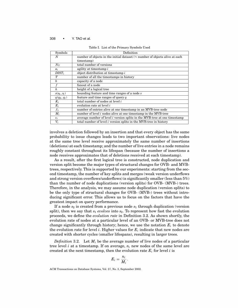
Table I. List of the Primary Symbols Used
Symbols DefinitionN number of objects in the initial dataset (≈ number of objects alive at each
timestamp)NV total number of versionsai agility at timestamp iDISTi object distribution at timestamp iT number of all the timestamps in historyb capacity of a nodef fanout of a nodeh height of a logical trees(sk , st ) bounding feature and time ranges of a node sq(qk , qt ) feature and time ranges of query qKi total number of nodes at level iEi evolution rate at level if1 number of entries alive at one timestamp in an MVB-tree nodeMi number of level i nodes alive at one timestamp in the MVB-treevi average number of level i version splits in the MVB-tree at one timestampVi total number of level i version splits in the MVB-tree in history
involves a deletion followed by an insertion and that every object has the sameprobability to issue changes leads to two important observations: live nodesat the same tree level receive approximately the same number of insertions(deletions) at each timestamp; and the number of live entries in a node remainsroughly constant throughout its lifespan (because the number of insertions anode receives approximates that of deletions received at each timestamp).
As a result, after the first logical tree is constructed, node duplication andversion split become the major types of structural changes for OVB- and MVB-trees, respectively. This is supported by our experiments: starting from the sec-ond timestamp, the number of key splits and merges (weak version underflowsand strong version overflows/underflows) is significantly smaller (less than 5%)than the number of node duplications (version splits) for OVB- (MVB-) trees.Therefore, in the analysis, we may assume node duplication (version splits) tobe the only type of structural changes for OVB- (MVB-) trees without intro-ducing significant error. This allows us to focus on the factors that have thegreatest impact on query performance.
If a node s2 is created from a previous node s1 through duplication (versionsplit), then we say that s1 evolves into s2. To represent how fast the evolutionproceeds, we define the evolution rate in Definition 3.2. As shown shortly, theevolution rate of nodes at a particular level of an OVB- or MVB-tree does notchange significantly through history; hence, we use the notation Ei to denotethe evolution rate for level i. Higher values for Ei indicate that new nodes arecreated with shorter cycles (smaller lifespans), resulting in larger trees.
Definition 3.2. Let Mi be the average number of live nodes of a particulartree level i at a timestamp. If on average, ni new nodes of the same level arecreated at the next timestamp, then the evolution rate Ei for level i is
Ei = ni
Mi.
ACM Transactions on Database Systems, Vol. 27, No. 3, September 2002.
Overlapping and Multiversion Structures • 309
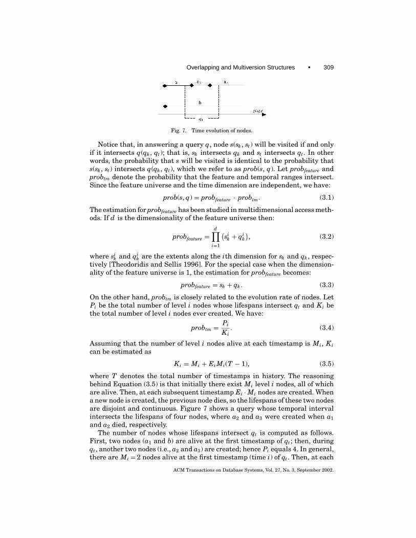
Fig. 7. Time evolution of nodes.
Notice that, in answering a query q, node s(sk , st) will be visited if and onlyif it intersects q(qk , qt); that is, sk intersects qk and st intersects qt . In otherwords, the probability that s will be visited is identical to the probability thats(sk , st) intersects q(qk , qt), which we refer to as prob(s, q). Let probfeature andprobtm denote the probability that the feature and temporal ranges intersect.Since the feature universe and the time dimension are independent, we have:
prob(s, q) = probfeature · probtm. (3.1)
The estimation for probfeature has been studied in multidimensional access meth-ods. If d is the dimensionality of the feature universe then:
probfeature =d∏
i=1
(sik + qi
k
), (3.2)
where sik and qi
k are the extents along the ith dimension for sk and qk , respec-tively [Theodoridis and Sellis 1996]. For the special case when the dimension-ality of the feature universe is 1, the estimation for probfeature becomes:
probfeature = sk + qk . (3.3)
On the other hand, probtm is closely related to the evolution rate of nodes. LetPi be the total number of level i nodes whose lifespans intersect qt and Ki bethe total number of level i nodes ever created. We have:
probtm = Pi
Ki. (3.4)
Assuming that the number of level i nodes alive at each timestamp is Mi, Kican be estimated as
Ki = Mi + Ei Mi(T − 1), (3.5)
where T denotes the total number of timestamps in history. The reasoningbehind Equation (3.5) is that initially there exist Mi level i nodes, all of whichare alive. Then, at each subsequent timestamp Ei ·Mi nodes are created. Whena new node is created, the previous node dies, so the lifespans of these two nodesare disjoint and continuous. Figure 7 shows a query whose temporal intervalintersects the lifespans of four nodes, where a2 and a3 were created when a1and a2 died, respectively.
The number of nodes whose lifespans intersect qt is computed as follows.First, two nodes (a1 and b) are alive at the first timestamp of qt ; then, duringqt , another two nodes (i.e., a2 and a3) are created; hence Pi equals 4. In general,there are Mi = 2 nodes alive at the first timestamp (time i) of qt . Then, at each
ACM Transactions on Database Systems, Vol. 27, No. 3, September 2002.
310 • Y. TAO et al.
of the subsequent timestamps i+ j (1≤ j ≤ |qt | −1), Ei ·Mi nodes are created.Hence, we have the following estimation for Pi.
Pi = Mi + Ei Mi(qt − 1). (3.6)
Combining Equations (3.4) through (3.6), we have
probtm =1+ Ei(qt − 1)1+ Ei(T − 1)
. (3.7)
Extending Equations (3.1) and (3.3), we derive:
prob(s, q) = (sk + qk)1+ Ei(qt − 1)1+ Ei(T − 1)
. (3.8)
Recall that prob(s, q) states the probability for a node to be accessed in answer-ing query q; thus the expected number of node accesses NA(q) is given by theequation:
NA(q) =∑
every node s
prob(s, q).
If si(sik , sit) are the average range and temporal extents of nodes at level i, theabove equation can be written as (3.9), where h denotes the height of a logicaltree, Ki denotes the total number nodes at level i, and prob(si, q) is given byEquation (3.8).
NA(q) =h−1∑i=0
[Ki ·prob(si, q)]. (3.9)
In this work, we assume each node in the tree occupies a single disk page;hence Equation (3.9) also gives the expected number of disk accesses. Obviously,the equation can be easily adapted to general cases where a node can occupymultiple pages. This cost model, however, is “qualitative”, in the sense that itmust refer to the corresponding tree to obtain values for the relevant variables.In the sequel, we aim at representing sik, Ei, Ki, and h using the properties ofthe indexed dataset and the underlying file system.
3.2 A Cost Model for OVB-Trees
In this section, we present the derivation of the cost model for OVB-treesthrough several steps. In each step, we focus on rewriting a particular compo-nent in Equation (3.9) as the function of variables whose values are obtainablewithout referring to the actual tree.
Estimating h. The height of a B-tree that indexes N keys is estimated asin Equation (3.10), where f is the fanout of the tree. The commonly adoptedvalue for f is ln 2 · bsplit [Yao 1978], where bsplit is the number of entries anode contains when it splits.3 For OVB-trees, bsplit= b. Note that since the node
3As shown in Yao [1978], the fanout of a node in the B-tree does not depend on the concrete datadistribution, but rather on the sequence of insertions. For example, the fanout is lowest if recordsare inserted in increasing order of their keys, and it is roughly the same for randomized insertions.Our cost models are based on randomized insertions because they are most common in practice.
ACM Transactions on Database Systems, Vol. 27, No. 3, September 2002.

Overlapping and Multiversion Structures • 311
capacity is decided by the page size of the underlying file system, the value off is independent of the indexed dataset. Furthermore, since each logical treeindexes the same number of objects, the height of each tree is expected to bethe same.
h = dlog f N/be + 1. (3.10)
Estimating Ei. We start with the estimation for E0, the evolution rate atthe leaf level. Let us consider a leaf node s of a logical tree at an arbitrarytimestamp i. Recall that s will be copied to a new node at timestamp (i+ 1)if and only if any change (i.e., insertion or deletion) occurs in the node. Fora dataset with agility a, the total number of changes per timestamp equals2aN because each object update involves one deletion and one insertion. E0corresponds to the probability that a leaf node is affected by any of these 2aNchanges. A leaf node contains on average N/ f entries. Given an update, everynode has the same probability f /N to be affected; thus, the probability for anode not to be affected by a single change is (1− f /N ). Since all the changesare independent, the probability for a node not to be updated by any of thesechanges is (1− f /N )2aN . Thus we have:
E0 = 1−(
1− fN
)2aN
. (3.11)
In general, the number of nodes at level i is N/ f i+ 1; hence the likelihood fora level i node to be affected by a change is f i+1/N . Following the derivation of(3.11), we obtain:
Ei = 1−(
1− f i+1
N
)2aN
(0≤ i≤h− 1). (3.12)
If N is sufficiently large (which is true in practice), we have
Ei ≈ 1− (1− e)2af i+1.
As a side product of the estimation for Ei, we have the following lemma forthe expected number of timestamps sit that a node at level i remains alive inhistory.
LEMMA 1. sit = 1/Ei.
PROOF. Consider a node s of level i that is created at timestamp k. Since theprobability that s is copied at one timestamp is Ei, it follows that the probabilitythat node s is valid for j timestamps (i.e., it is copied at timestamp k+ j ) is(1− Ei) j –1 · Ei. Therefore, the expected number of timestamps that node s isvalid in history is given by
∞∑j=1
{[Ei(1− Ei) j−1] · j
}.
The above series converges to 1/Ei.
Estimating Ki. Since, at level i, the number of live nodes at one timestampis N/ f i+1, the number of new nodes created at each timestamp is Ei · (N/ f i+1).
ACM Transactions on Database Systems, Vol. 27, No. 3, September 2002.
312 • Y. TAO et al.
Hence, the total number of level i nodes is
Ki = Nf i+1 + Ei
Nf i+1 (T − 1) (0≤ i≤h− 1). (3.13)
Note that a corollary of Equation (3.13) is that we can estimate the size of anOVB-tree as
Size(OVB) =h−1∑i=0
Ki =h−1∑i=0
[N
f i+1 + EiN
f i+1 (T − 1)]. (3.14)
Estimating sik . Now it remains to estimate sik , the average key range ofnodes at level i. Notice that, since each logical tree is simply an ordinary B-tree,this estimation is directly obtainable from the analysis of B-trees. In fact, whenDIST is uniform, the key ranges of nodes at the same level are roughly thesame. Given that there are N/ f i+1 nodes at level i in a B+-tree, we have
sik = f i+1
N(0 ≤ i ≤ h− 1). (3.15)
So far we have rewritten all the components of Equation (3.9) as functionsof f , N , a, and T . The number of node accesses for OVB-trees is presented inEquation (3.16).
NA(q) =dlog f N/be∑
i=0
[N
f i+1 + EiN
f i+1 (T − 1)](
f i+1
N+ qk
)1+ Ei(qt − 1)1+ Ei(T − 1)
=dlog f N/be∑
i=0
Nf i+1
(f i+1
N+ qk
)[1+
(1−
(1− f i+1
N
)2aN)(qt − 1)
].
(3.16)
Note that when a equals 0, the above equation degenerates into a cost modelfor conventional B-trees.
3.3 A Cost Model for MVB-Trees
In the sequel, we carry out a similar analysis for MVB-trees based onEquation (3.9).
Estimating h. Let f1 be the average number of live entries at a single times-tamp in node s. Note that f1 is different from f , which equals the total numberof entries in s. Thus, the height of a logical tree is given by Equation (3.17):
h = dlog f1N/be. (3.17)
Meanwhile, let Mi denote the average number of level i nodes that are alive ata single timestamp in a logical tree. The estimation for Mi is
Mi = N
f i+11
(0≤ i≤h− 1).
The estimation for f1 deserves further elaboration. Recall that, in MVB-trees,if a node consists of only entries at the same timestamp, then the number of
ACM Transactions on Database Systems, Vol. 27, No. 3, September 2002.
Overlapping and Multiversion Structures • 313
the entries cannot exceed b ·PSVO; otherwise a strong version overflow occursand the node will be key split. Hence, f1= ln 2 · bsplit= ln 2 · b · PSVO.
Estimating Ei. We first present the estimation for E0. A node s containsf1 entries when it is created from a version split; thus s will receive (b− f1)insertions before it generates a version split, which in turn leads to the creationof a new node. At each timestamp, as there are a ·N insertions, each leaf nodecan receive on average a ·N/M0 insertions. As a result, s will generate a versionsplit after (b− f1) ·M0/(a ·N ) timestamps. Since M0=N/ f1, the number oftimestamps s0t that a leaf level node remains alive before it is version split, canbe estimated as
s0t = (b− f1)M0
aN= b− f1
af1.
Let Vi be the total number (in history) of version splits at level i, and vi theaverage number of version splits per timestamp at level i. For the leaf level, V0and v0 are estimated as
V0 = M0T − 1
s0t= aN (T − 1)
b− f1, and v0 = V0
T − 1= aN
b− f1.
Recall that the evolution rate is defined as the number of new nodes over thetotal number of live nodes at a timestamp. Since version splits are the only typeof structural changes considered, we have
E0 = v0
M0= af1
b− f1.
Whenever a leaf node generates a version split, an entry will be inserted intoits parent node at level 1. Hence, at each timestamp, the average number ofinsertions at level 1 is v0, and every level 1 node receives on average v0/M1entries. Similar to our analysis above, a node at level 1 will generate a versionsplit (b− f1) ·M1/v0 timestamps after its creation. Therefore, the lifespan ofthe node, s1t is
s1t = (b− f1) M1
v0= (b− f1)2
af 21
.
The estimation for V1 is
V1 = M1T − 1
s1t= aN (T − 1)
(b− f1)2 .
In the same way, we obtain the following equations for nodes at higher levels.
sit = (b− f1)i+1
af i+11
, and Vi = aN (T − 1)(b− f1)i+1 (0 ≤ i ≤ h− 1). (3.18)
Hence, we have
vi = Vi
T − 1= aN
(b− f1)i+1 , and Ei = vi
Mi= af i+1
1
(b− f1)i+1 (0 ≤ i ≤ h− 1).
(3.19)
ACM Transactions on Database Systems, Vol. 27, No. 3, September 2002.
314 • Y. TAO et al.
Finally, note that, as with Lemma 1 for OVB-trees, sit = 1/Ei also applies tonodes of MVB-trees at all levels.
Estimating Ki. Given that the total number of version splits at level i isprovided by Equation (3.18), the total number Ki of nodes created throughhistory is:
Ki = Mi + Vi = N
f i+11
+ aN(T − 1
)(b− f1)i+1 (0 ≤ i ≤ h− 1). (3.20)
As a corollary of Equation (3.20), the size of an MVB-tree can be estimated as
Size(MVB) =h−1∑i=0
Ki =h−1∑i=0
[N
f i+11
+ aN (T − 1)(b− f1)i+1
]. (3.21)
Estimating sik. As mentioned above, a node contains f1 live entries at thesame timestamp. Therefore, replacing f in Equation (3.15) for OVB-trees withf1, we obtain the following equation for the average key range of nodes at level i.
sik = f i+11
N(0 ≤ i ≤ h− 1). (3.22)
Equation (3.23) presents the final model, which predicts the node disk ac-cesses for range-interval queries based on the properties of the indexed datasetand the underlying file system.
NA(q) =dlog f1 N/be∑
i=0
[N
f i+11
+ EiN
f i+11
(T − 1)](
f i+11
N+ qk
)1+ Ei(qt − 1)1+ Ei(T − 1)
=dlog f1 N/be∑
i=0
N
f i+11
(f i+1
1
N+ qk
)[1+ af i+1
1 · (qt − 1)(b− f1)i+1
]. (3.23)
Tuning PSVO. Recall that a MVB-tree has several tree parameters, amongwhich PSVO (i.e., the strong version overflow threshold) has the most significanteffect on the overall performance of the tree.4 To understand this, observe fromEquations (3.21) and (3.23) that both the tree size and query performance arevery closely related to f1, which, as mentioned earlier, can be approximatedas ln 2 · b · PSVO. Our models provide useful insight towards choosing a goodvalue for PSVO. For example, according to Equation (3.21) setting a low PSVO(which in turn makes f1 smaller) usually reduces the tree size, by decreasingthe term (aN (T − 1))/((b− f1)i+ 1), which corresponds to the number of nodescreated after the first timestamp, and will eventually dominate the other termN/ f i+1
1 (i.e., the number of nodes that are alive only at the first timestamp).Intuitively, a smaller f1 allows a node to receive more entries before it is versionsplit, which reduces the total number of version splits, and hence data redun-dancy. However, if PSVO is too low, the height of the tree (see Equation (3.17)
4Usually the other parameters are defined based on PSVO, for example, PSVU= PSVO/2,PU = PSVO/4 [Varman and Verma 1997].
ACM Transactions on Database Systems, Vol. 27, No. 3, September 2002.
Overlapping and Multiversion Structures • 315
will become significantly higher, which, as shown in the experiments, may in-crease the total tree size if the number of nodes created at higher levels (duringthe entire history) exceeds the number of nodes diminished at lower levels.Furthermore, a high tree may compromise query performance. In fact, we ob-serve that for any specific query parameters qk and qt , there exists an optimalPSVO that minimizes the query cost NA(q), and can be obtained by solving PSVOfrom the equation,
d [NA(q)]df1
· df1
dPSVO= 0,
where NA(q) is given by Equation (3.23). When qt = 1 (timestamp queries), forexample, the optimal PSVO equals the maximum value 1, which means thatstrong version overflows can never happen. This is expected because a times-tamp query only needs to search one logical B-tree; thus it is important tomaximize the fanout f1 of each logical tree. Queries with longer intervals havebest performance with smaller PSVO so that the resulting tree has less redun-dancy (due to the fact that version splits happen less often). These observationsare verified by the experiments.
3.4 Selectivity Estimation
A record i with feature ik and lifespan it , will be retrieved by a query q, ifand only if q(qk , qt) intersects i(ik , it). The probability prob(i, q) for i(ik , it) andq(qk , qt) to intersect is calculated according to Equation (3.8), except that theevolution rate of the objects now corresponds to the agility a of the dataset, andik is set to 0 because the feature of each entry indexed by an OVB- or MVB-treecontains only a single value. Hence, we have:
sel(q) = prob(i, q) = qk1+ a(qt − 1)1+ a(T − 1)
. (3.24)
As a result, the number NUM(q) of records retrieved by query q is estimated as
NUM(q) = prob(i, q) · [N + aN(T − 1)] = N ·qk · [1+ a(qt − 1)]. (3.25)
3.5 Asymptotical Performance of Interval Queries
As mentioned earlier, traditional analysis on MLTS focused on their asymptot-ical performance for timestamp queries. Both structures achieve the optimalquery cost, namely, O(log(NV /b)+ K /b) node accesses, and the space consump-tion is O(NV /b) (optimal) for MVB-trees and O(NV log(N/b)) (suboptimal) forOVB-trees, where NV is the total number of versions produced by N objectsthroughout the history, K the number of versions retrieved, and b the nodecapacity. No result, however, exists for the asymptotical performance of eitherstructure on interval queries. Particularly, since the MVB-tree is optimal (bothin space and query cost) for timestamp queries, an interesting problem is tostudy whether it is also optimal for interval queries or, equivalently, whetherit answers any interval query that returns K versions in O(log(NV /b)+ K /b)node accesses.
ACM Transactions on Database Systems, Vol. 27, No. 3, September 2002.
316 • Y. TAO et al.
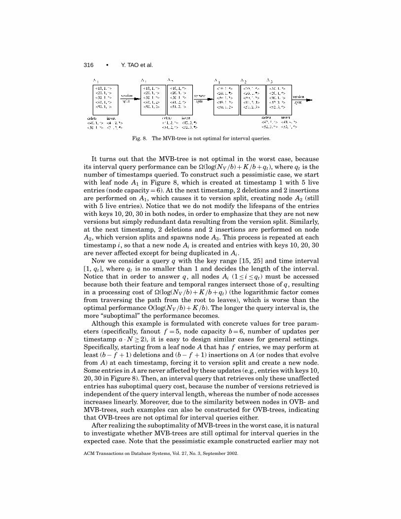
Fig. 8. The MVB-tree is not optimal for interval queries.
It turns out that the MVB-tree is not optimal in the worst case, becauseits interval query performance can be Ä(log(NV /b)+ K /b+qt), where qt is thenumber of timestamps queried. To construct such a pessimistic case, we startwith leaf node A1 in Figure 8, which is created at timestamp 1 with 5 liveentries (node capacity= 6). At the next timestamp, 2 deletions and 2 insertionsare performed on A1, which causes it to version split, creating node A2 (stillwith 5 live entries). Notice that we do not modify the lifespans of the entrieswith keys 10, 20, 30 in both nodes, in order to emphasize that they are not newversions but simply redundant data resulting from the version split. Similarly,at the next timestamp, 2 deletions and 2 insertions are performed on nodeA2, which version splits and spawns node A3. This process is repeated at eachtimestamp i, so that a new node Ai is created and entries with keys 10, 20, 30are never affected except for being duplicated in Ai.
Now we consider a query q with the key range [15, 25] and time interval[1, qt], where qt is no smaller than 1 and decides the length of the interval.Notice that in order to answer q, all nodes Ai (1≤ i≤qt) must be accessedbecause both their feature and temporal ranges intersect those of q, resultingin a processing cost of Ä(log(NV /b)+ K /b+qt) (the logarithmic factor comesfrom traversing the path from the root to leaves), which is worse than theoptimal performance O(log(NV /b)+ K /b). The longer the query interval is, themore “suboptimal” the performance becomes.
Although this example is formulated with concrete values for tree param-eters (specifically, fanout f = 5, node capacity b= 6, number of updates pertimestamp a ·N ≥ 2), it is easy to design similar cases for general settings.Specifically, starting from a leaf node A that has f entries, we may perform atleast (b− f + 1) deletions and (b− f + 1) insertions on A (or nodes that evolvefrom A) at each timestamp, forcing it to version split and create a new node.Some entries in A are never affected by these updates (e.g., entries with keys 10,20, 30 in Figure 8). Then, an interval query that retrieves only these unaffectedentries has suboptimal query cost, because the number of versions retrieved isindependent of the query interval length, whereas the number of node accessesincreases linearly. Moreover, due to the similarity between nodes in OVB- andMVB-trees, such examples can also be constructed for OVB-trees, indicatingthat OVB-trees are not optimal for interval queries either.
After realizing the suboptimality of MVB-trees in the worst case, it is naturalto investigate whether MVB-trees are still optimal for interval queries in theexpected case. Note that the pessimistic example constructed earlier may not
ACM Transactions on Database Systems, Vol. 27, No. 3, September 2002.
Overlapping and Multiversion Structures • 317
necessarily happen in the expected case, because it is rather unlikely that anobject will remain unchanged for a long period of time if every object has thesame probability to issue updates. To be specific, we may check if the estimatednumber of node accesses NA (produced from Equation (3.23) is indeed boundedby O(log(NV /b)+ K /b), where K denotes the number of versions retrieved (pro-duced from (3.25). As shown shortly, when N ·qk ≥ f1 the expected performanceof MVB-trees is indeed optimal for interval queries by employing the query al-gorithm in Bercken and Seeger [1996], which, as mentioned in Section 2.2, onlyvisits the nonleaf nodes whose lifespans intersect the first timestamp of thequery, as well as all the leaf nodes whose feature and temporal extents inter-sect those of the query. The cost of visiting the nonleaf nodes corresponds to thelogarithmic term log(NV /b) of the optimal complexity. In the sequel, we showthat the expected number NA0 of leaf node accesses is bounded by O(K /b).
To illustrate this, observe that, since Ei =a · f i1/(b− f1)i, and f1= ln 2 ·
b ·Psvo, we have: Ei =a · (ln 2 ·Psvo)i/(1− ln 2 ·Psvo)i, leading to the fact thatEi =O(a) (since PSVO is a constant). This means that the evolution rate of MVB-trees at any level is as fast (in terms of complexity) as the data agility, which issomewhat against the intuition that nodes at higher levels should evolve moreslowly than nodes at lower levels (i.e., with longer lifespans). In fact, notice thatfor some Psvo (specifically when ln 2 ·Psvo> 1/2) the evolution rates at higherlevels can be even higher than those at lower levels. Formally, NA0 is estimatedfrom Equation (3.23),
NA0 = Nf1
(f1
N+ qk
)[1+ E0(qt − 1)] =
(1+ N
f1qk
)[1+ E0(qt − 1)]
= 1+ Nf1
qk + E0(qt − 1)+ Nf1
qk · E0(qt − 1). (3.26)
Because f1=O(b) and Ei =O(a), NA0 is bounded by (when N ·qk ≥ f1)
NA0 = O[
Nb
qk + Nb
qk ·a(qt − 1)].
Since K =N ·qk +N ·qk ·a(qt − 1), we have NA0=O(K /b). Combining withthe fact that the number of nonleaf node accesses establishes the logarith-mic term O(log(NV /b)), the overall expected performance of MVB-trees isbounded by O(log(NV /b)+ K /b). Recall that this bound is achieved by assum-ing N ·qk ≥ f1, which is required so that the term E0(qt − 1) is absorbed by(N/ f1) ·qk · E0(qt − 1) in the big-O complexity of Equation (3.26). Note that thisextra condition ensures that the feature range qk of the query is at least as longas the average feature range f1/N of a leaf node. When this is not satisfied(consider, for instance, the pessimistic example given in Figure 8), the querycost may be bounded by E0(qt − 1), which, intuitively, indicates that the numberof versions retrieved by the query is not sufficient for justifying the nodes thatevolved during the qt and must be accessed by the query.
Next we conduct a similar analysis for the interval query performance ofOVB-trees. However, instead of showing their expected optimality (which ascan be conjectured is not true), we aim at quantifying the factor by which theirexpected performance deviates from the optimal cost. Similarly, we assume the
ACM Transactions on Database Systems, Vol. 27, No. 3, September 2002.
318 • Y. TAO et al.
algorithm proposed in Bercken and Seeger [1996] so that the total numberof nonleaf node accesses corresponds to the logarithmic factor O(log(NV /b)),allowing us to focus on the leaf node accesses. To facilitate analysis we assumeN is large so that
E0 = 1− (1− f /N )2aN ≈ 1− e−2af .
Furthermore, we observe that for typical values of f (on the order of 100 for reg-ular disk pages), e−2af ≈ 0; thus E0≈ 1. From Equation (3.16) we have (similarto MVB-trees, assuming N ·qk ≥ f ):
NA0 = Nf
(fN+ qk
)[1+ E0(qt − 1)] =
(1+ N
fqk
)[1+ E0(qt − 1)]
= O[1+ N
fqk + (qt − 1)+ N
fqk · (qt − 1)
]= O
[Nb
qk + Nb
qk · 1a a(qt − 1)]
= 1a
O[a
Nb
qk + Nb
qk ·a(qt − 1)]
= 1a
O[
Nb
qk + Nb
qk ·a(qt − 1)]= 1
aO(
Kb
).
Therefore, it is clear that the performance of OVB-trees is closely related to thedata agility a (which is not the case for MVB-trees). As a increases, OVB-treesapproach the optimal performance. Consider, for example, the extreme casewhere a= 1 (i.e., all objects change at every timestamp). Then, maintaining aseparate B-tree at each timestamp is an optimal solution in the sense that thenumber of node accesses is linear to the number of object versions retrieved. Infact, as discussed in the next section and shown in the experiments, OVB-treesactually outperform MVB-trees beyond certain agility.
3.6 Predicting the Behavior of MLTS
The proposed models can answer two important questions: when it is worthusing a MLTS instead of the independent-tree implementation (i.e., an indi-vidual B-tree for each timestamp), and which MLTS is preferable dependingon structure size and query performance considerations. Regarding the firstquestion, notice that when the agility exceeds a certain threshold (which wecall the degradation agility), all the live nodes will be duplicated (version split)in an overlapping (multiversion) structure, at each timestamp; that is, bothstructures will degenerate into independent trees. To calculate the degrada-tion agility, notice that a MLTS degrades completely when the evolution rateEi approaches 1 for all levels, where Ei is defined in (3.12) and (3.19) for OVB-and MVB-trees, respectively. Solving these equations, we obtain the degrada-tion agilities for OVB- and MVB-trees as follows.
deg-agility(OVB) ≈ −1N log(1− f /N )
. (3.27)
deg-agility(MVB) ≈ b− f1
f1= 1− ln 2 · Psvo
ln 2 · Psvo. (3.28)
ACM Transactions on Database Systems, Vol. 27, No. 3, September 2002.
Overlapping and Multiversion Structures • 319
For OVB-trees the estimated degradation agility is very low (less than 5% forour experimental settings), which severely limits their applicability. In orderto intuitively explain this phenomenon, consider a situation where the aver-age fanout of OVB-trees is f = 100. Even if one (out of 100) object in a nodeissues a change, the node needs to be copied (which leads to replication of all100 entries). Furthermore, the update may lead to an insertion in another node,which will lead to duplication of that node as well. Therefore, in the worst case,even if less than 1% of the objects issue updates at a timestamp, an OVB-treemay degenerate to independent B-trees. Furthermore, the degradation agilitybecomes even lower for larger block sizes.
On the other hand, although the estimated degradation agility of MVB-treesis more than an order of magnitude higher (about 80% for our settings) this doesnot mean that MVB-trees are better than ephemeral B-trees up to this value ofagility. Recall that each entry in a multiversion structure contains additionalinformation about its lifespan, which lowers the node fanout. As a result, al-though an MVB-tree may have not degraded, above an agility threshold, whichwe call size multitree point (MTP, for short), it consumes more space than theindependent-tree implementation. The size MTP can be predicted by solving thefollowing equation, where the right part corresponds to the size of independentB-trees.
Size(MVB) = T ·dlog f Ne−1∑
i=0
Nf i+1 ,
Size(MVB) is given in Equation (3.21), and f is the fanout of a B- (or OVB-)tree. Solving this equation we obtain:
aMTP(size) ≈(
Tf− 1
f1
)· bMVB − f1
T − 1≈ bMVB(1− ln 2 · PSVO)
f(3.29)
where bMVB is the node capacity of the MVB-tree.Similarly, for certain query parameters (qk , qt), we can also calculate the
query MTP (the agility above which independent B-trees outperform the MVB-tree) by solving Equation (3.30). Although the query and size MTPs are notnecessarily identical (the query MTP depends on the query parameters), theirvalues, as shown in the experimental evaluation, are usually very close.
NA(q) = qt ·dlog f N/be∑
i=0
Nf i+1
(f i+1
N+ qk
)
⇒ aMTP (qk , qt) ≈1+ qk ·N/ f1+ qk ·N/ f1
qt − 1
PSVO · ln 21− PSVO · ln 2
(qt − 1). (3.30)
The above equation holds for qt > 1 (i.e., interval queries). For timestampqueries, the query MTP is meaningless, because the independent-tree imple-mentation (or OVB-tree) always outperforms MVB-trees due to their larger
ACM Transactions on Database Systems, Vol. 27, No. 3, September 2002.
320 • Y. TAO et al.
fanouts. For interval queries and large values of N , Equation (3.30) can besimplified to
aMTP (qk , qt) ≈f1
fqt − 1
PSVO · ln 21− PSVO · ln 2
(qt − 1).
Furthermore, when qt is sufficiently high (i.e., long interval queries), the queryMTP converges to
aMTP (qk , qt) ≈(1− PSVO · ln 2
)f1
PSVO · ln 2 · f.
For agilities below the query MTP, MVB-trees are usually more efficient forinterval queries. Furthermore, the performance gain over OVB-trees can be ob-tained by considering Equations (3.16) and (3.23). Let NAi(OVB) and NAi(MVB)denote the number of node accesses at level i in answering query q with an OVB-and MVB-tree, respectively. Then, we have
NAi(OVB)NAi(MVB)
≈ 1+ EOi (qt − 1)1+ EMi (qt − 1)
·C(qk), (3.31)
where C(qk) is a function of qk , and EOi and EMi correspond to the evolution ratesat level i for the OVB- and MVB-tree, respectively. Given that typically EOi isan order of magnitude larger than EMi, the ratio in the above equation initiallyincreases with qt (for small qt and fixed qk) and will converge to EOi ·C(qk)/EMiwhen qt is sufficiently large. These observations are experimentally evaluatedin Section 5.
4. GENERALIZATION OF THE ANALYSIS FRAMEWORK
The models of the previous section assume that no buffer is available, and thedatasets are uniform whereas the agility remains constant for each timestamp.Section 4.1 extends the cost models to estimate page accesses in the presence ofLRU buffers, and Section 4.2 addresses general data distributions and variableagilities. Finally, Section 4.3 applies the entire analysis framework to R-trees.
4.1 Introducing a LRU Buffer
Equations (3.16) and (3.23) estimate the number of node accesses of OVB- andMVB-trees. In practical environments, buffers are widely used to improve queryefficiency, and ignoring the effect of buffering may bias performance evaluation.Therefore, it is important for the proposed models to capture the number of diskpage accesses when a (typically, LRU) buffer is available.
The behavior of LRU buffers in general database environments has been an-alyzed in Bhide et al. [1993]. Subsequent work [Huang et al. 1997; Leuteneggerand Lopez 2000] that addresses the buffered performance of specific index struc-tures is based on Bhide et al.’s [1993] findings that, after the buffer warmupperiod (i.e., all buffer pages have been loaded), the probability of locating a pagein the buffer does not vary significantly. Based on this idea, Leutenegger and
ACM Transactions on Database Systems, Vol. 27, No. 3, September 2002.
Overlapping and Multiversion Structures • 321
Lopez [2000] adopt a two-step approach to predict the I/O of access methods.Assuming an empty buffer with C pages, the first step aims at estimating thenumber nq of queries performed when all C pages are loaded. Let prob(si, q)denote the probability that a node at level i is accessed by a query; then theprobability that a level i node is accessed at least once by any of the nq queriesis: 1− [1− prob(si, q)]nq . Since the total number of distinct pages accessed afternq queries is C (recall that at this point the buffer becomes full for the firsttime), nq can be solved from the following equation (Ki is the total number ofnodes at level i).
dlog f N/be∑i=0
(Ki ·
{1− [1− prob (si, q)]nq
}) = C. (4.1)
After obtaining nq (which in practice can be saved in the system log), the secondstep estimates the number of page accesses for answering query q by observingthat a node needs to be fetched from the disk if and only if the following condi-tions are satisfied: (1) the extents of the node intersect those of the query (forwhich the probability is prob(si, q) for a node at level i), and (2) the node is not inthe buffer. According to Bhide et al. [1993], the probability of (2) approximatesthe probability that the node is not accessed by any of the nq queries during thebuffer warmup period. Since this probability is [1− prob(si, q)]nq for a level inode, the probability for the node to be loaded from the disk (to answer queryq) is given by prob(si, q) · (1− prob(si, q))nq . Therefore, the number of disk pageaccesses PA(q) is given by
PA(q) =dlog f N/be∑
i=0
{Ki ·prob(si, q) · [1− prob(si, q)]nq
}. (4.2)
Finally, Ki and prob(si, q) for OVB- and MVB-trees have already been discussedin the last section. Specifically, Ki is given in Equations (3.13) and (3.20), whilefor prob(si, q):
OVB prob(si, q) =(
f i+1
N+ qk
)1+ Ei
(qt − 1
)1+ Ei
(T − 1
)
=(
f i+1
N+ qk
) 1+[
1−(
1− f i+1
N
)2aN] (qt − 1
)1+
[1−
(1− f i+1
N
)2aN] (T − 1
) ;
(4.3)
MVB prob(si, q) =(
f i+11
N+ qk
)1+ Ei(qt − 1)1+ Ei(T − 1)
=(
f i+11
N+ qk
)1+ af i+1
1 · (qt − 1)(b− f1)i+1
1+ af i+11 · (T − 1)(b− f1)i+1
. (4.4)
ACM Transactions on Database Systems, Vol. 27, No. 3, September 2002.

322 • Y. TAO et al.
Fig. 9. A histogram example.
Applying the above equations in (4.1) and (4.2), we obtain cost models thatpredict the number of page accesses in answering a query with OVB- and MVB-trees when the buffer contains C pages.
4.2 General Temporal Datasets
In order to capture general temporal datasets, we need to allow arbitrary dis-tributions and variable agilities for each timestamp. In practice, arbitrary datadistributions are usually described using histograms, the idea of which is todivide the feature universe into a set of partitions such that the feature dis-tribution of the objects within each partition is (almost) uniform [Piatetsky-Shapiro and Connell 1984; Liption et al. 1990]. Figure 9 illustrates an examplewhere four partitions A, B, C, D are allocated. Each partition is associatedwith certain statistical information: typically, the number of features in thepartition and the partition length. For example, there are five features in A,whose length is l A. The histogram is used to estimate the selectivity of a query,or equivalently, the number of features to be retrieved. Consider, for example,the query in Figure 9 whose feature range intersects partitions A and B (withintersection lengths a and b). Given that A and B contain 5 and 4 features,respectively, the number of features retrieved can be estimated as: 5 · (a/l A)+4 · (b/l B).
The description for data agility ai, on the other hand, is straightforward:we only need to store a sequence of numbers representing the values of ai ateach timestamp. Observe that although values of ai may differ significantly,consecutive DISTi are usually very similar (e.g., the balance distribution of ac-counts changes slowly from one timestamp to the next one). Since most queriesin practice involve short intervals [Salzberg and Tsotras 1999], it is reasonableto consider that DISTi remains approximately the same at all timestamps iduring qt , which indicates that logical trees at these timestamps have similarstructures.
Next we extend the analysis of Section 3 to address general temporaldatasets. Without loss of generality, we denote the set of query timestampsas t1, t2, . . . , tqt. Let Nε be the number of features retrieved at the first times-tamp t1. Since DISTi does not vary significantly5 during qt , approximately thesame number of features is retrieved at every timestamp ti (1≤ i ≤ qt). Let S1 bethe set of nodes that are accessed at t1 (i.e., these nodes are alive at t1 and their
5In some extreme cases where distributions change drastically in consecutive timestamps, we canuse the average number of features retrieved at each timestamp to replace Nε .
ACM Transactions on Database Systems, Vol. 27, No. 3, September 2002.

Overlapping and Multiversion Structures • 323
feature ranges intersect qk). Because logical trees at close timestamps have sim-ilar structures, nodes that evolve from those in S1 at subsequent timestampshave similar feature ranges. As a result, the complete set of nodes accessed bya query is approximately the union of S1 and the set SE of nodes evolving fromS1 during qt , or more formally, NA(q) = |S1|+ |SE |. If Nεi is the number of leveli nodes in S1, then:
|S1| =h−1∑i=0
Nεi.
Given Nε (obtained from histograms), the values for Nεi can be computed byobserving that a range query on B-trees must visit a set of nodes whose featureranges are consecutive. Since on average f entries are reported in each leafnode (with possible exceptions for the two nodes whose feature ranges includethe endpoints of the query range), the number of expected leaf nodes accessedis [Nε/ f ]. Following the same reasoning: Nεi = max{1, [Nε/ f i+1]} (the maxoperation is due to the fact that at least one node must be visited at each leveleven if no record is retrieved; that is, Nε = 0).
Next we focus on |SE |, for which we need to estimate the evolution rateEεi for level i nodes in S1. Unlike Ei in Section 3, Eεi is a function of time(represented as Eεi( j ) for timestamp j ) because the number of updates at eachtimestamp is different. Then the number of level i nodes that evolve from S1during qt is given by Nεi
∑tqtj=t2
Eεi( j ). So the total number of nodes in SE is∑h−1i=0 [Nεi
∑tqtj=t2
Eεi ( j )]. As a result,
NA(q) = |S1| + |SE | =h−1∑i=0
Nεi
1+tqt∑
j=t2
Eεi ( j )
.The derivation of Eεi follows that of Ei as presented in Section 3, except that,
since we only consider a fraction of live nodes (specifically, Nεi) at each times-tamp, the number of updates that affect these nodes is aj ·Nεi · f i+1 (note thatNεi · f i+1 is the number of entries in the subtrees of the Nεi nodes). Therefore,for OVB-trees,
Eεi ( j ) = 1−(
1− 1Nεi
)2aj ·Nεi · f i+1
. (4.5)
The new cost model that estimates the number of node accesses for OVB-trees is
OVB NA(q) =dlog f N/be∑
i=0
Nεi
1+tqt∑
j=t2
[1−
(1− 1
Nεi
)2aj ·Nεi · f i+1].
(4.6)
Similarly, for MVB-trees, the evolution rate Eεi( j ) at timestamp j is given by
Eεi ( j ) = aj · f i+11
(b− f1)i+1 . (4.7)
ACM Transactions on Database Systems, Vol. 27, No. 3, September 2002.
324 • Y. TAO et al.
The corresponding formula for MVB-trees is
MVB NA(q) =dlog f1 N/be∑
i=0
Nεi
1+f i+1
1 ·j=tqt−1∑
j=t2
aj
(b− f1)i+1
. (4.8)
The size estimation of OVB- and MVB-trees is the same as the uniform case,except that agility ai (hence, Ei) may vary at each timestamp. The estimationsfor Ei( j ) (i.e., the evolution rate of level i at timestamp j ) is similar to Equations(4.5) and (4.7), but the number of updates at each timestamp is a ·N . ReplacingEi · (T − 1) with
∑Tj=2 Ei( j )in Equations (3.14) and (3.21), we obtain:
Size(OVB) =dlog f N/be∑
i=0
(N
f i+1
{1+
T−1∑i=2
[1−
(1− f i+1
N
)2ai N]}); (4.9)
Size(MVB) =dlog f1 N/be∑
i=0
N
f i+11
+N ·
T−1∑i=2
ai
(b− f1)i+1
. (4.10)
Following the analysis of Section 3.4, the estimation for selectivity becomes:
NUM(q) = Nε ·(
1+tqt∑
i=t2
ai
), and sel(q) =
Nε ·(
1+tqt∑
i=t2
ai
)
N ·(
1+T−1∑i=2
ai
) . (4.11)
Finally, we extend Equation (4.2) to capture the query performance when aLRU buffer is available. First observe that the expected number of disk pageaccesses PA(q) can be written as
PA(q) =h−1∑i=0
Nεi
1+tqt∑
j=t2
Eεi ( j )
· [1− probε(si, q)]nq
, (4.12)
where probε(si, q) is the probability (averaged “locally,” namely, among nodesin |S1| and |SE |) that a node of level i is accessed by the query. The reason-ing of the above equation is that Nεi[1+
∑tqtj=t2
Eεi ( j )] is the number of nodesthat must be accessed at level i, and [1−probε(si, q)]nq states the average prob-ability that each of these nodes is not in the buffer (thus it must be fetchedfrom the disk). We estimate probε(si, q) based on Equation (3.8) except thatsk and Ei are replaced with the corresponding locally averaged values. Morespecifically:
sk = (Nεi · f i+1) · qk
Nε
, and Ei = 1qt − 1
tqt∑j=t2
Eεi ( j ),
ACM Transactions on Database Systems, Vol. 27, No. 3, September 2002.

Overlapping and Multiversion Structures • 325
where Eεi is given in Equations (4.5) and (4.7), respectively, for OVB- andMVB-trees.
4.3 Extension to General MLTS
The previous analysis consists of two parts: probfeature and probtm (seeEquation (3.1). The properties of B-trees are only used for probfeature, or morespecifically, sik (the feature extent of a node). Extensions of the cost models toother MLTS differ only in the estimation of probfeature, because general MLTSare constructed through the same overlapping or multiversion frameworks, andthus have similar temporal behavior. Therefore, provided that related resultsare available regarding the performance of an ephemeral structure, our frame-work produces models for the resulting MLTS easily. In the sequel, we illustratethis by considering the R-tree as the ephemeral structure; that is, the corre-sponding MLTS are overlapping R-trees (OVR-trees) and multiversion R-trees(MVR-trees).6
R-trees have been extensively used in spatial databases, where the universeis a two dimensional square. By Equation (3.2), probfeature should be repre-sented as
probfeature = (s1 + q1)(s2 + q2), (4.13)
where q1 and q2 are the extents of qk along the spatial dimensions.The cost models for OVR- and MVR-trees differ from those for OVB- and
MVB-trees only in the estimation for s1 and s2, which is the focus of R-treeanalysis [Kamel and Faloutsos 1993; Pagel and Six 1996; Theodoridis and Sellis1996; Theodoridis et al. 2000]. Particularly, when DIST is uniform, the estima-tion is given by Equations (4.14) and (4.15), where Di refers to the density ofnode MBRs at level i (D0 is the density D of the actual object MBRs).7
si1 = si2 =√
Di+1f i+1
N(0 ≤ i ≤ h− 1) (4.14)
where
Di+1 =(
1+√
Di − 1√f
)2
and D0 = D. (4.15)
Replacing sik with si1 and si2 in Equations (3.16) and (3.23), we obtain the costmodels for OVR- and MVR-trees as in Equations (4.16) and (4.17) respectively.
6As mentioned earlier, existing implementations of OVR- and MVR-trees are HR- [Nascimento andSilva 1998] and BTR-trees [Kumar et al. 1998], respectively.7The density of a set of rectangles is defined as the average number of rectangles that contain agiven point in the workspace. Equivalently, density can be expressed as the ratio of the sum ofthe areas of all rectangles over the area of the available workspace. Equations (4.14) and (4.15)assume that the MBRs of nodes in R-trees are quadratic, which is a widely accepted fact in R-treecost analysis [Pagel and Six 1996; Theodoridis and Sellis 1996].
ACM Transactions on Database Systems, Vol. 27, No. 3, September 2002.
326 • Y. TAO et al.
Similarly, (4.18) and (4.19) compute the tree sizes, and Equation (4.20) predictsthe selectivity of interval queries. Note that the notions of degradation agilityand multitree point apply to general MLTS by following the same reasoning asfor B-trees.
OVR NA(q) =dlog f Ne−1∑
i=0
Nf i+1
√Di+1f i+1
N+ q1
√Di+1f i+1
N+ q2
×{
1+[
1−(
1− f i+1
Nε
)2aj ·Nε]
(qt − 1)
}). (4.16)
MVR NA(q) =dlog f1
Ne−1∑i=0
N
f i+11
√Di+1f i+1
1
N+ q1
√Di+1f i+1
1
N+ q2
×[
1+ af i+11 · (qt − 1)(b− f1)i+1
]}. (4.17)
Size(OVR) =dlog f Ne−1∑
i=0
Ki =h−1∑i=0
{N
f i+1 +[
1−(
1− f i+1
Nε
)2aj ·Nε]
× Nf i+1 (T − 1)
}. (4.18)
Size(MVR) =dlog f1 Ne−1∑
i=0
Ki =h−1∑i=0
[N
f i+11
+ af i+11 N (T − 1)(b− f1)i+1
]. (4.19)
sel(q) =(√
DN+ q1
)(√DN+ q2
)1+ a(qt − 1)1+ a(T − 1)
. (4.20)
Extending the above models to address performance under buffers and arbi-trary data distribution is also straightforward. Specifically, prob(si, q) is esti-mated as Equations (4.21) and (4.22), respectively, for OVR- and MVR-trees.Replacing prob(si, q) in Equation (4.2) with these two equations we obtain mod-els that predict the number of page accesses.
OVR prob(si, q) =√Di+1
f i+1
N+ q1
√Di+1f i+1
N+ q2
×1+
[1−
(1− f i+1
N
)2aN] (qt − 1
)1+
[1−
(1− f i+1
N
)2aN] (T − 1
) . (4.21)
ACM Transactions on Database Systems, Vol. 27, No. 3, September 2002.
Overlapping and Multiversion Structures • 327
OVR prob(si, q) =√Di+1
f i+11
N+ q1
√Di+1f i+1
1
N+ q2
×
1+ af i+1
1 · (qt − 1)(b− f1)i+1
1+ af i+11 · (T − 1)(b− f1)i+1
. (4.22)
Arbitrary data distribution (particularly query selectivity) can be accuratelycaptured by extending the histogram methods for 1-D features. By applying theanalysis in Section 4.1, we obtain equations that have exactly the same form asEquations (4.6) and (4.8) through (4.12) for query performance and tree size ofOVR- and MVR-trees, as well as the query selectivity. The difference is in theway that values of Nε and Nei are obtained, which is the topic of the analysisof R-trees [Acharya et al. 1999; Theodoridis et al. 2000].
Our cost models assume that MLTS are searched in a recursive depth-firstmanner. That is, if all the branches of a node have been visited, we backtrackto the parent node and continue with the next qualifying nontraversed branch.In spite of the fact that, as mentioned earlier, specialized algorithms (i.e., back-ward pointers [Bercken and Seeger 1996]) may improve the performance ofinterval queries, we chose to present our model using the recursive depth-firstalgorithm for the following reasons. First, the backward pointer method appliesonly to a few ephemeral structures. For others (e.g., R-tree based structures), itis necessary to visit qualifying entries at all levels. Since we aim at the generalmethodology, we based our derivation on the recursive algorithm. Second, itis straightforward to adapt the proposed models to the backward pointer al-gorithm: the estimation for the leaf nodes remains the same, whereas we onlyneed to set qt to 1 to obtain estimations for the other levels.
5. EXPERIMENTAL EVALUATION
In this section, we conduct an extensive experimental evaluation to prove the ef-ficiency of the proposed models, first discussing MLTS based on B-trees. Due tothe lack of real datasets, we created synthetic ones as follows. At the first times-tamp, the features (each feature is a single value) of 20K objects distribute inthe universe [0, 1] following uniform, skewed (i.e., Zipf with harmonic constant0.6), or Gaussian (with mean 0.5, variance 0.2) distributions. Then, at eachof the following 199 timestamps (i.e., the history contains 200 timestamps),a% of the objects are selected to produce feature changes (a ranges from 0 to100%). For example, if a equals 25%, 5K (= 25%× 20K) objects issue updatesper timestamp and the entire dataset contains 1 million (= 5K× 200) records.Each feature update is such that the feature of an object deviates from its pre-vious value by a distance randomly generated in [−0.05, 0.05]. In this way, weallow the distribution of the objects’ features to vary slowly along with time.Figure 10 shows the histograms at timestamps 1, 100, and 200 for datasetswith the same agility a= 10% but different initial distribution DIST1. Noticethat as time evolves the data distribution gradually becomes uniform. In order
ACM Transactions on Database Systems, Vol. 27, No. 3, September 2002.
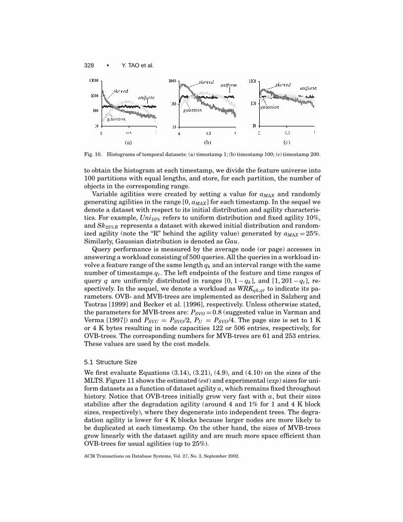
328 • Y. TAO et al.
Fig. 10. Histograms of temporal datasets: (a) timestamp 1; (b) timestamp 100; (c) timestamp 200.
to obtain the histogram at each timestamp, we divide the feature universe into100 partitions with equal lengths, and store, for each partition, the number ofobjects in the corresponding range.
Variable agilities were created by setting a value for aMAX and randomlygenerating agilities in the range [0, aMAX] for each timestamp. In the sequel wedenote a dataset with respect to its initial distribution and agility characteris-tics. For example, Uni10% refers to uniform distribution and fixed agility 10%,and Sk25%R represents a dataset with skewed initial distribution and random-ized agility (note the “R” behind the agility value) generated by aMAX= 25%.Similarly, Gaussian distribution is denoted as Gau.
Query performance is measured by the average node (or page) accesses inanswering a workload consisting of 500 queries. All the queries in a workload in-volve a feature range of the same length qk and an interval range with the samenumber of timestamps qt . The left endpoints of the feature and time ranges ofquery q are uniformly distributed in ranges [0, 1−qk], and [1, 201−qt], re-spectively. In the sequel, we denote a workload as WRKqk,qt to indicate its pa-rameters. OVB- and MVB-trees are implemented as described in Salzberg andTsotras [1999] and Becker et al. [1996], respectively. Unless otherwise stated,the parameters for MVB-trees are: PSVO= 0.8 (suggested value in Varman andVerma [1997]) and PSVU = PSVO/2, PU = PSVO/4. The page size is set to 1 Kor 4 K bytes resulting in node capacities 122 or 506 entries, respectively, forOVB-trees. The corresponding numbers for MVB-trees are 61 and 253 entries.These values are used by the cost models.
5.1 Structure Size
We first evaluate Equations (3.14), (3.21), (4.9), and (4.10) on the sizes of theMLTS. Figure 11 shows the estimated (est) and experimental (exp) sizes for uni-form datasets as a function of dataset agility a, which remains fixed throughouthistory. Notice that OVB-trees initially grow very fast with a, but their sizesstabilize after the degradation agility (around 4 and 1% for 1 and 4 K blocksizes, respectively), where they degenerate into independent trees. The degra-dation agility is lower for 4 K blocks because larger nodes are more likely tobe duplicated at each timestamp. On the other hand, the sizes of MVB-treesgrow linearly with the dataset agility and are much more space efficient thanOVB-trees for usual agilities (up to 25%).
ACM Transactions on Database Systems, Vol. 27, No. 3, September 2002.
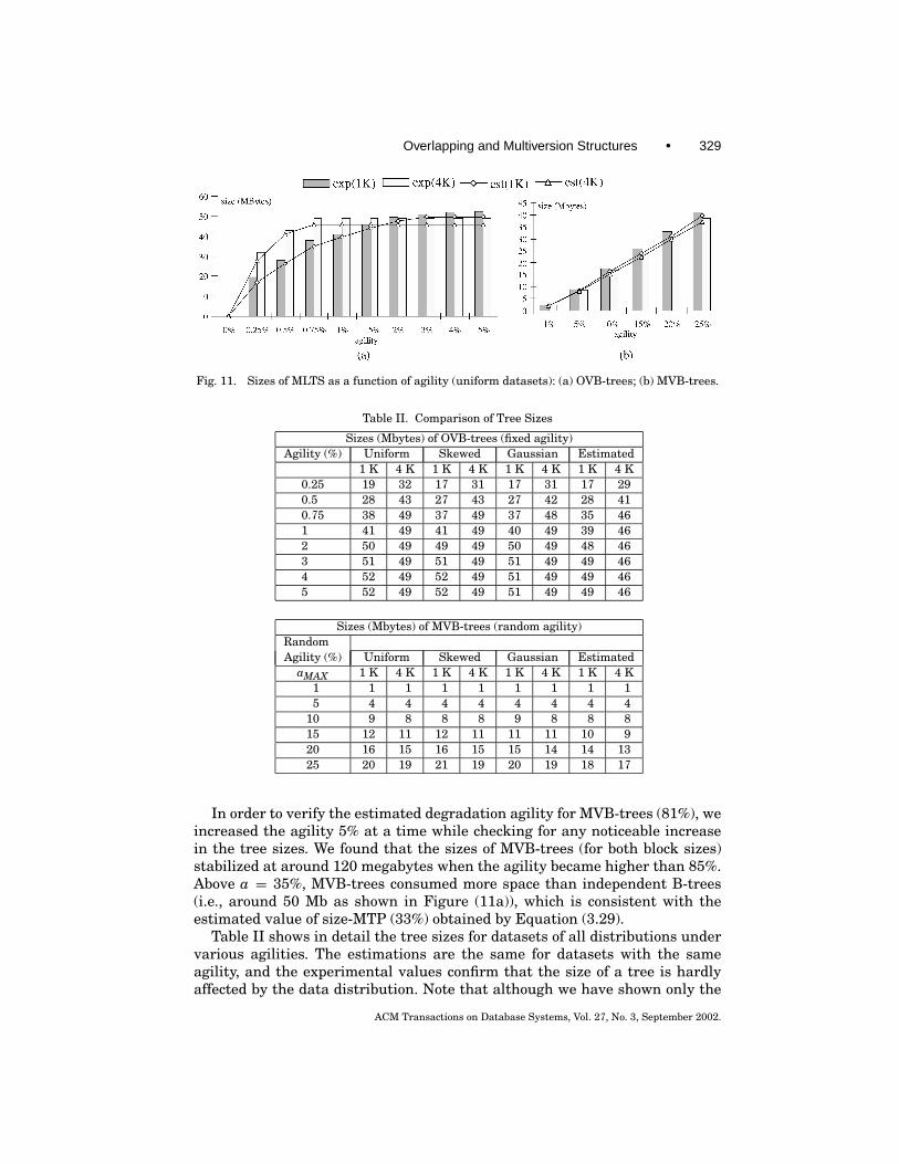
Overlapping and Multiversion Structures • 329
Fig. 11. Sizes of MLTS as a function of agility (uniform datasets): (a) OVB-trees; (b) MVB-trees.
Table II. Comparison of Tree Sizes
Sizes (Mbytes) of OVB-trees (fixed agility)Agility (%) Uniform Skewed Gaussian Estimated
1 K 4 K 1 K 4 K 1 K 4 K 1 K 4 K0.25 19 32 17 31 17 31 17 290.5 28 43 27 43 27 42 28 410.75 38 49 37 49 37 48 35 461 41 49 41 49 40 49 39 462 50 49 49 49 50 49 48 463 51 49 51 49 51 49 49 464 52 49 52 49 51 49 49 465 52 49 52 49 51 49 49 46
Sizes (Mbytes) of MVB-trees (random agility)RandomAgility (%) Uniform Skewed Gaussian Estimated
aMAX 1 K 4 K 1 K 4 K 1 K 4 K 1 K 4 K1 1 1 1 1 1 1 1 15 4 4 4 4 4 4 4 4
10 9 8 8 8 9 8 8 815 12 11 12 11 11 11 10 920 16 15 16 15 15 14 14 1325 20 19 21 19 20 19 18 17
In order to verify the estimated degradation agility for MVB-trees (81%), weincreased the agility 5% at a time while checking for any noticeable increasein the tree sizes. We found that the sizes of MVB-trees (for both block sizes)stabilized at around 120 megabytes when the agility became higher than 85%.Above a = 35%, MVB-trees consumed more space than independent B-trees(i.e., around 50 Mb as shown in Figure (11a)), which is consistent with theestimated value of size-MTP (33%) obtained by Equation (3.29).
Table II shows in detail the tree sizes for datasets of all distributions undervarious agilities. The estimations are the same for datasets with the sameagility, and the experimental values confirm that the size of a tree is hardlyaffected by the data distribution. Note that although we have shown only the
ACM Transactions on Database Systems, Vol. 27, No. 3, September 2002.
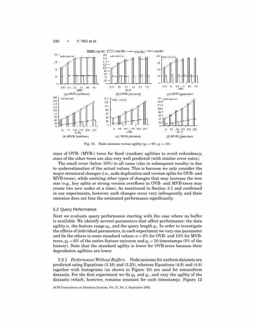
330 • Y. TAO et al.
Fig. 12. Node accesses versus agility (qk = 6%, qt = 10).
sizes of OVB- (MVB-) trees for fixed (random) agilities to avoid redundancy,sizes of the other trees are also very well predicted (with similar error rates).
The small error (below 10%) in all cases (also in subsequent results) is dueto underestimation of the actual values. This is because we only consider themajor structural changes (i.e., node duplication and version splits for OVB- andMVB-trees), while omitting other types of changes that may increase the treesize (e.g., key splits or strong version overflows in OVB- and MVB-trees maycreate two new nodes at a time). As mentioned in Section 3.1 and confirmedin our experiments, however, such changes occur very infrequently, and theiromission does not bias the estimated performance significantly.
5.2 Query Performance
Next we evaluate query performance starting with the case where no bufferis available. We identify several parameters that affect performance: the dataagility a, the feature range qk , and the query length qt . In order to investigatethe effects of individual parameters, in each experiment we vary one parameterand fix the others to some standard values: a= 2% for OVB- and 10% for MVB-trees, qk = 6% of the entire feature universe and qt = 10 timestamps (5% of thehistory). Note that the standard agility is lower for OVB-trees because theirdegradation agilities are lower.
5.2.1 Performance Without Buffers. Node accesses for uniform datasets arepredicted using Equations (3.16) and (3.23), whereas Equations (4.6) and (4.8)together with histograms (as shown in Figure 10) are used for nonuniformdatasets. For the first experiment we fix qk and qt , and vary the agility of thedatasets (which, however, remains constant for each timestamp). Figure 12
ACM Transactions on Database Systems, Vol. 27, No. 3, September 2002.
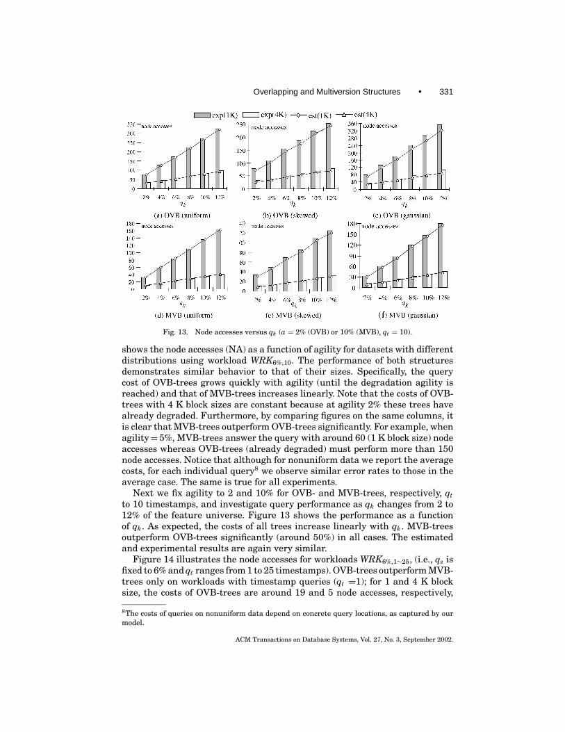
Overlapping and Multiversion Structures • 331
Fig. 13. Node accesses versus qk (a = 2% (OVB) or 10% (MVB), qt = 10).
shows the node accesses (NA) as a function of agility for datasets with differentdistributions using workload WRK6%,10. The performance of both structuresdemonstrates similar behavior to that of their sizes. Specifically, the querycost of OVB-trees grows quickly with agility (until the degradation agility isreached) and that of MVB-trees increases linearly. Note that the costs of OVB-trees with 4 K block sizes are constant because at agility 2% these trees havealready degraded. Furthermore, by comparing figures on the same columns, itis clear that MVB-trees outperform OVB-trees significantly. For example, whenagility= 5%, MVB-trees answer the query with around 60 (1 K block size) nodeaccesses whereas OVB-trees (already degraded) must perform more than 150node accesses. Notice that although for nonuniform data we report the averagecosts, for each individual query8 we observe similar error rates to those in theaverage case. The same is true for all experiments.
Next we fix agility to 2 and 10% for OVB- and MVB-trees, respectively, qtto 10 timestamps, and investigate query performance as qk changes from 2 to12% of the feature universe. Figure 13 shows the performance as a functionof qk . As expected, the costs of all trees increase linearly with qk . MVB-treesoutperform OVB-trees significantly (around 50%) in all cases. The estimatedand experimental results are again very similar.
Figure 14 illustrates the node accesses for workloads WRK6%,1∼25, (i.e., qs isfixed to 6% and qt ranges from 1 to 25 timestamps). OVB-trees outperform MVB-trees only on workloads with timestamp queries (qt =1); for 1 and 4 K blocksize, the costs of OVB-trees are around 19 and 5 node accesses, respectively,
8The costs of queries on nonuniform data depend on concrete query locations, as captured by ourmodel.
ACM Transactions on Database Systems, Vol. 27, No. 3, September 2002.
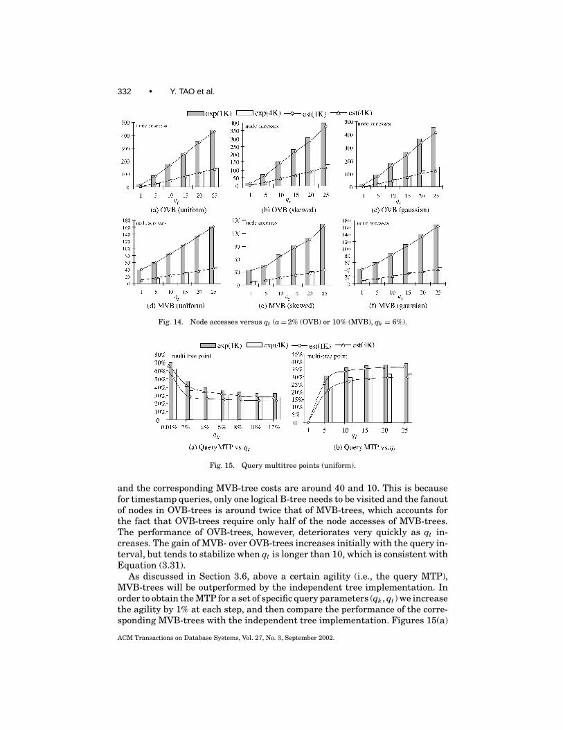
332 • Y. TAO et al.
Fig. 14. Node accesses versus qt (a= 2% (OVB) or 10% (MVB), qk = 6%).
Fig. 15. Query multitree points (uniform).
and the corresponding MVB-tree costs are around 40 and 10. This is becausefor timestamp queries, only one logical B-tree needs to be visited and the fanoutof nodes in OVB-trees is around twice that of MVB-trees, which accounts forthe fact that OVB-trees require only half of the node accesses of MVB-trees.The performance of OVB-trees, however, deteriorates very quickly as qt in-creases. The gain of MVB- over OVB-trees increases initially with the query in-terval, but tends to stabilize when qt is longer than 10, which is consistent withEquation (3.31).
As discussed in Section 3.6, above a certain agility (i.e., the query MTP),MVB-trees will be outperformed by the independent tree implementation. Inorder to obtain the MTP for a set of specific query parameters (qk , qt) we increasethe agility by 1% at each step, and then compare the performance of the corre-sponding MVB-trees with the independent tree implementation. Figures 15(a)
ACM Transactions on Database Systems, Vol. 27, No. 3, September 2002.
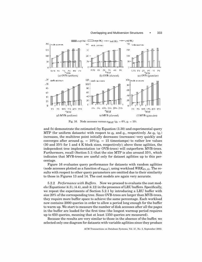
Overlapping and Multiversion Structures • 333
Fig. 16. Node accesses versus aMAX (qk = 6%, qt = 10).
and (b) demonstrate the estimated (by Equation (3.30) and experimental queryMTP (for uniform datasets) with respect to qk and qt , respectively. As qk (qt)increases, the multitree point initially decreases (increases) very quickly andconverges after around qk = 10%(qt = 15 timestamps) to rather low values(30 and 35% for 1 and 4 K block sizes, respectively); above these agilities, theindependent tree implementation (or OVB-trees) will outperform MVB-trees.Furthermore, recall (Section 5.1) that the size MTP is also around 35%, whichindicates that MVB-trees are useful only for dataset agilities up to this per-centage.
Figure 16 evaluates query performance for datasets with random agilities(node accesses plotted as a function of aMAX), using workload WRK6%,10. The re-sults with respect to other query parameters are omitted due to their similarityto those in Figures 13 and 14. The cost models are again very accurate.
5.2.2 Performance with Buffers. Now we proceed to evaluate the cost mod-els (Equations (4.3), (4.4), and (4.12) in the presence of LRU buffers. Specifically,we repeat the experiments of Section 5.2.1 by introducing a LRU buffer withsize 20% of the corresponding tree. Since OVB-trees are larger than MVB-trees,they require more buffer space to achieve the same percentage. Each workloadnow contains 2000 queries in order to allow a period long enough for the bufferto warm up. We start to measure the number of disk accesses after all the pagesin the buffer are loaded for the first time (the longest warmup period requiresup to 650 queries, meaning that at least 1350 queries are measured).
Because the results are very similar to those in the absence of the buffer, weselected only one diagram for datasets with variable agilities since they produce
ACM Transactions on Database Systems, Vol. 27, No. 3, September 2002.
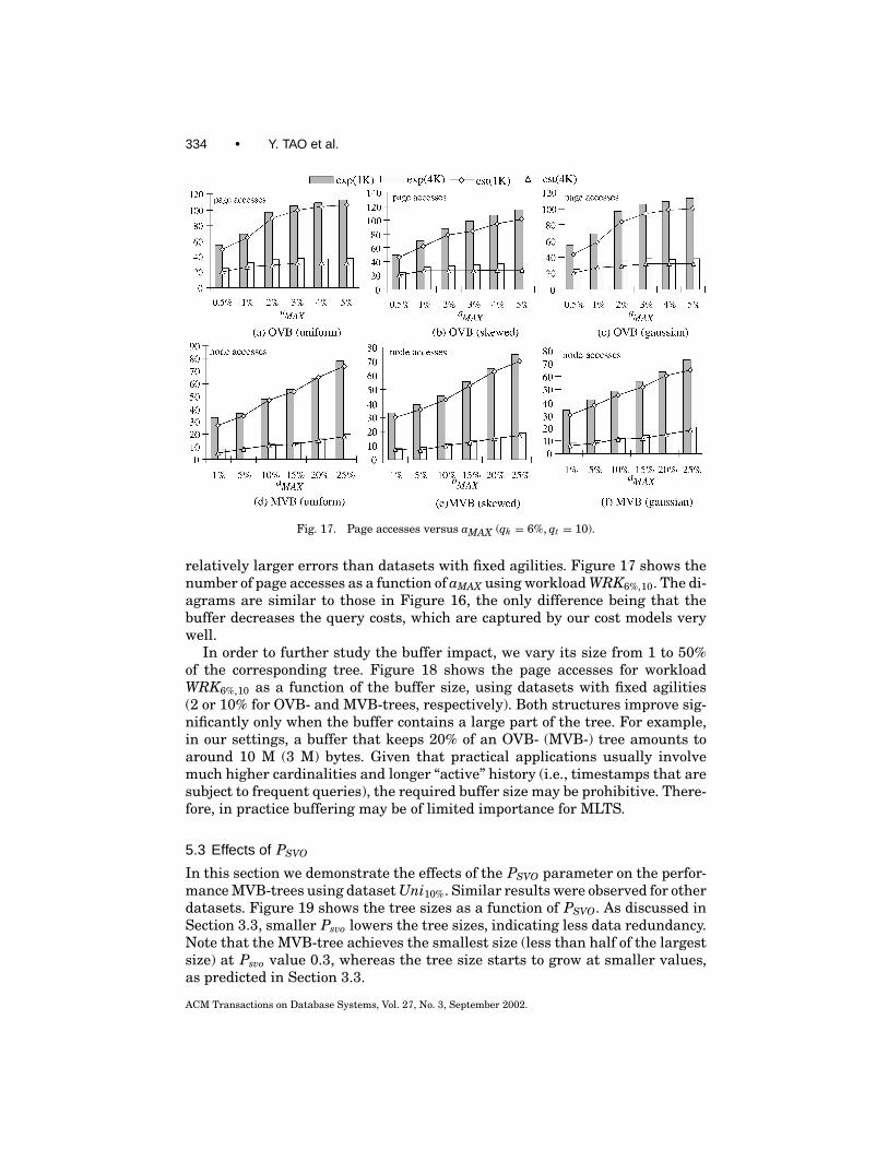
334 • Y. TAO et al.
Fig. 17. Page accesses versus aMAX (qk = 6%, qt = 10).
relatively larger errors than datasets with fixed agilities. Figure 17 shows thenumber of page accesses as a function of aMAX using workload WRK6%,10. The di-agrams are similar to those in Figure 16, the only difference being that thebuffer decreases the query costs, which are captured by our cost models verywell.
In order to further study the buffer impact, we vary its size from 1 to 50%of the corresponding tree. Figure 18 shows the page accesses for workloadWRK6%,10 as a function of the buffer size, using datasets with fixed agilities(2 or 10% for OVB- and MVB-trees, respectively). Both structures improve sig-nificantly only when the buffer contains a large part of the tree. For example,in our settings, a buffer that keeps 20% of an OVB- (MVB-) tree amounts toaround 10 M (3 M) bytes. Given that practical applications usually involvemuch higher cardinalities and longer “active” history (i.e., timestamps that aresubject to frequent queries), the required buffer size may be prohibitive. There-fore, in practice buffering may be of limited importance for MLTS.
5.3 Effects of PSVO
In this section we demonstrate the effects of the PSVO parameter on the perfor-mance MVB-trees using dataset Uni10%. Similar results were observed for otherdatasets. Figure 19 shows the tree sizes as a function of PSVO. As discussed inSection 3.3, smaller Psvo lowers the tree sizes, indicating less data redundancy.Note that the MVB-tree achieves the smallest size (less than half of the largestsize) at Psvo value 0.3, whereas the tree size starts to grow at smaller values,as predicted in Section 3.3.
ACM Transactions on Database Systems, Vol. 27, No. 3, September 2002.
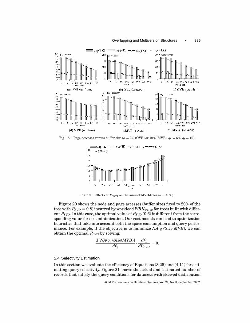
Overlapping and Multiversion Structures • 335
Fig. 18. Page accesses versus buffer size (a = 2% (OVB) or 10% (MVB), qk = 6%, qt = 10).
Fig. 19. Effects of PSVO on the sizes of MVB-trees (a = 10%).
Figure 20 shows the node and page accesses (buffer sizes fixed to 20% of thetree with PSVO = 0.8) incurred by workload WRK6%,10 for trees built with differ-ent PSVO. In this case, the optimal value of PSVO (0.6) is different from the corre-sponding value for size minimization. Our cost models can lead to optimizationheuristics that take into account both the space consumption and query perfor-mance. For example, if the objective is to minimize NA(q)/Size(MVB), we canobtain the optimal PSVO by solving:
d [NA(q)/Size(MVB)]df1
· df1
dPSVO= 0.
5.4 Selectivity Estimation
In this section we evaluate the efficiency of Equations (3.25) and (4.11) for esti-mating query selectivity. Figure 21 shows the actual and estimated number ofrecords that satisfy the query conditions for datasets with skewed distribution
ACM Transactions on Database Systems, Vol. 27, No. 3, September 2002.
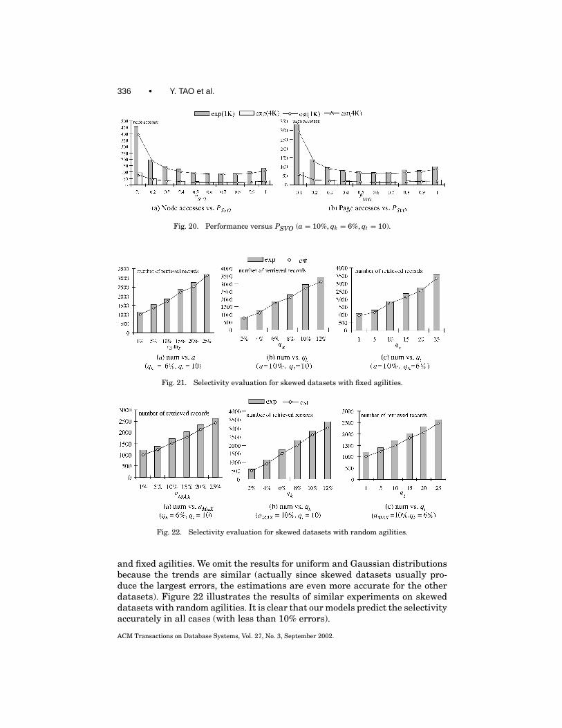
336 • Y. TAO et al.
Fig. 20. Performance versus PSVO (a = 10%, qk = 6%, qt = 10).
Fig. 21. Selectivity evaluation for skewed datasets with fixed agilities.
Fig. 22. Selectivity evaluation for skewed datasets with random agilities.
and fixed agilities. We omit the results for uniform and Gaussian distributionsbecause the trends are similar (actually since skewed datasets usually pro-duce the largest errors, the estimations are even more accurate for the otherdatasets). Figure 22 illustrates the results of similar experiments on skeweddatasets with random agilities. It is clear that our models predict the selectivityaccurately in all cases (with less than 10% errors).
ACM Transactions on Database Systems, Vol. 27, No. 3, September 2002.
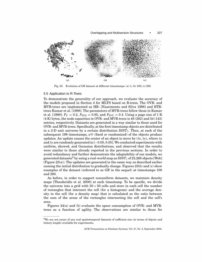
Overlapping and Multiversion Structures • 337
Fig. 23. Evolution of GR dataset at different timestamps: (a) 1; (b) 100; (c) 200.
5.5 Application to R-Trees
To demonstrate the generality of our approach, we evaluate the accuracy ofthe models proposed in Section 4 for MLTS based on R-trees. The OVR- andMVR-trees are implemented as HR- [Nascimento and Silva 1998] and BTR-trees Kumar et al. [1998]. The parameters of MVR-trees follow those in Kumaret al. [1998]: PU = 0.2, PSVO = 0.85, and PSVU = 0.4. Using a page size of 1 K(4 K) bytes, the node capacities in OVR- and MVR-trees is 48 (202) and 34 (143)entries, respectively. Datasets are generated in a way similar to those used forOVB- and MVB-trees. Specifically, at the first timestamp objects are distributedin a 2-D unit universe by a certain distribution DIST1. Then, at each of thesubsequent 199 timestamps, a% (fixed or randomized) of the objects produceupdates. An update causes the center of an object to move by (δx, δy), where δxand δy are randomly generated in [−0.05, 0.05]. We conducted experiments withuniform, skewed, and Gaussian distributions, and observed that the resultswere similar to those already reported in the previous sections. In order toavoid redundancy and further demonstrate the adaptability of our models, wegenerated datasets9 by using a real-world map as DIST1 of 23,268 objects [Web](Figure 23(a)). The updates are generated in the same way as described earliercausing the initial distribution to gradually change. Figures 23(b) and (c) showexamples of the dataset (referred to as GR in the sequel) at timestamps 100and 200.
As before, in order to support nonuniform datasets, we maintain densitymaps [Theodoridis et al. 2000] at each timestamp. To be specific, we dividethe universe into a grid with 50× 50 cells and store in each cell the numberof rectangles that intersect the cell (for a histogram) and the average den-sity in the cell (for a density map) that is calculated as the ratio betweenthe sum of the areas of the rectangles intersecting the cell and the cell’sarea.
Figures 24(a) and (b) evaluate the space consumption of OVR- and MVR-trees as a function of agility. The observations are similar to those for
9We are not aware of any real spatiotemporal datasets of sufficient size (in terms of objects andhistory length) available for experiments.
ACM Transactions on Database Systems, Vol. 27, No. 3, September 2002.
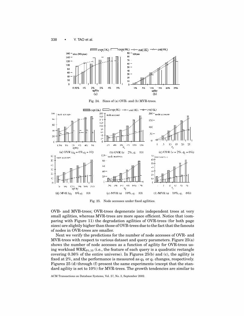
338 • Y. TAO et al.
Fig. 24. Sizes of (a) OVR- and (b) MVR-trees.
Fig. 25. Node accesses under fixed agilities.
OVB- and MVB-trees; OVR-trees degenerate into independent trees at verysmall agilities, whereas MVR-trees are more space efficient. Notice that (com-paring with Figure 11) the degradation agilities of OVR-trees (for both pagesizes) are slightly higher than those of OVB-trees due to the fact that the fanoutsof nodes in OVR-trees are smaller.
Next we verify the predictions for the number of node accesses of OVR- andMVR-trees with respect to various dataset and query parameters. Figure 25(a)shows the number of node accesses as a function of agility for OVR-trees us-ing workload WRK6%,10 (i.e., the feature of each query is a quadratic rectanglecovering 0.36% of the entire universe). In Figures 25(b) and (c), the agility isfixed at 2%, and the performance is measured as qk or qt changes, respectively.Figures 25 (d) through (f) present the same experiments (except that the stan-dard agility is set to 10%) for MVR-trees. The growth tendencies are similar to
ACM Transactions on Database Systems, Vol. 27, No. 3, September 2002.
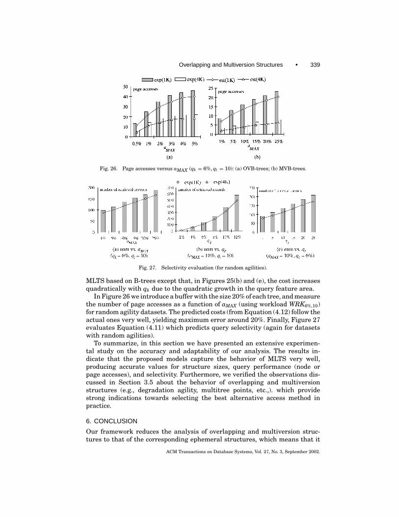
Overlapping and Multiversion Structures • 339
Fig. 26. Page accesses versus aMAX (qk = 6%, qt = 10): (a) OVB-trees; (b) MVB-trees.
Fig. 27. Selectivity evaluation (for random agilities).
MLTS based on B-trees except that, in Figures 25(b) and (e), the cost increasesquadratically with qk due to the quadratic growth in the query feature area.
In Figure 26 we introduce a buffer with the size 20% of each tree, and measurethe number of page accesses as a function of aMAX (using workload WRK6%,10)for random agility datasets. The predicted costs (from Equation (4.12) follow theactual ones very well, yielding maximum error around 20%. Finally, Figure 27evaluates Equation (4.11) which predicts query selectivity (again for datasetswith random agilities).
To summarize, in this section we have presented an extensive experimen-tal study on the accuracy and adaptability of our analysis. The results in-dicate that the proposed models capture the behavior of MLTS very well,producing accurate values for structure sizes, query performance (node orpage accesses), and selectivity. Furthermore, we verified the observations dis-cussed in Section 3.5 about the behavior of overlapping and multiversionstructures (e.g., degradation agility, multitree points, etc.,). which providestrong indications towards selecting the best alternative access method inpractice.
6. CONCLUSION
Our framework reduces the analysis of overlapping and multiversion struc-tures to that of the corresponding ephemeral structures, which means that it
ACM Transactions on Database Systems, Vol. 27, No. 3, September 2002.

340 • Y. TAO et al.
is applicable to a variety of different access methods. Extensive experimenta-tion proves the precision of the models for a wide range of conditions. To thebest of our knowledge, this is the first work that attempts to provide a system-atic study for these types of structures. Given the ever-increasing availabilityand importance of historical data in numerous applications, analysis of relatedstructures is crucial for the development of efficient systems.
In addition to their usefulness for query optimization, the proposed modelsprovide significant insight into the behavior of overlapping and multiversionstructures. In particular, we establish, for the first time, the close connectionbetween the performance of MLTS and the dataset agility. Furthermore, the for-mulae quantify how fast redundant data accumulate and predict the agilitieswhere the structures degrade to independent trees. In general, multiversionstructures usually incur less redundancy than overlapping structures and arepreferable for general workloads. Above a certain agility (multitree points),however, the best alternative is to simply build an independent ephemeralstructure for each timestamp. The proposed models accurately estimate thedegradation agilities and the multitree points. Thus they can be employed bysystem administrators to decide suitable indexing methods given the datasetand system characteristics.
Furthermore, this article also lays down a solid foundation for investigatingthe performance of other queries, such as temporal and spatiotemporal joins[Soo et al. 1994; Zhang et al. 2002]; aggregate queries [Yang and Widom 2001;Papadias et al. 2002; Zhang et al 2001; Tao et al. 2002], and spatiotemporalnearest neighbor queries. It may also lead to the development of improvedaccess methods. For example, structures such as MVB-trees were motivated bythe need to optimize timestamp queries with minimal space overhead. Otherstructures could be developed aiming at the optimization of interval queries,balancing the tradeoff between data redundancy and performance.
REFERENCES
ACHARYA, S., POOSALA, V., AND RAMASWAMY, S. 1999. Selectivity estimation in spatial databases. InProceedings of the ACM SIGMOD Conference (June), 13–24.
BECKER, B., GSCHWIND, S., OHLER, T., SEEGER, B., AND WIDMAYER, P. 1996. An asymptotically optimalmultiversion B-tree. VLDB J. 5, 4, 264–275.
BERCKEN, J. V. D. AND SEEGER, B. 1996. Query processing techniques for multiversion accessmethods. In Proceedings of the VLDB Conference (Sept.), 168–179.
BHIDE, A., DAN, A., AND DIAS, D. 1993. A simple analysis of LRU buffer replacement policy andits relationship to buffer warm-up transient. In Proceedings of the International Conference ofData Engineering (ICDE) (April), 125–133.
BURTON, F. AND HUNTBACH, M. 1985. Multiple generation text files using overlapping tree.Comput. J. 28, 4, 414–416.
BURTON, F., KOLLIAS, J., KOLLIAS, V., AND MATSAKIS, D. 1990. Implementation of overlapping B-treesfor time and space efficient representation of collection of similar files. Comput. J. 33, 3, 279–280.
CAREY, M., DEWITT, D., RICHARDSON, J., AND SHEKITA, E. 1986. Object and file management in theEXODUS extensible database system. In Proceedings of the VLDB Conference (August), 91–100.
CHIEN, S., TSOTRAS, V., ZANIOLO, C., AND ZHANG, D. 2002. Efficient complex query support for mul-tiversion XML documents. In Proceedings of the Extending Database Technology Conference(EDBT) (March), 161–178.
EASTON, M. 1986. Key-sequence data sets on indelible storage. IBM J. Res. Dev. 30, 3, 230–241.
ACM Transactions on Database Systems, Vol. 27, No. 3, September 2002.
Overlapping and Multiversion Structures • 341
GARGANTINI, I. 1982. An efficient way to represent quadtrees. Commun. ACM 25, 12, 905–910.GUTTMAN, A. 1984. R-trees: A dynamic index structure for spatial searching. In Proceedings of
the ACM SIGMOD Conference (June), 47–57.HUANG, Y., JING, N., AND RUNDENSTEINER, E. 1997. A cost model for estimating the performance of
spatial joins using R-trees. In Proceedings of the Scientific and Statistical Database ManagementConference (SSDBM) (August), 30–38.
JIANG, L., SALZBERG, B., LOMET, D., AND BARRENA, M. 2000. The BT-tree: A branched and temporalaccess method. In Proceedings of the VLDB Conference (Sept.), 451–460.
KAMEL, I. AND FALOUTSOS, C. 1993. On packing R-trees. In Proceedings of the Conference on Infor-mation and Knowledge Management (CIKM) (Nov.), 490–499.
KOLLIOS, G., GUNOPULOS, D., TSOTRAS, V., DELIS, A., AND HADJIELEFTHERIOU, M. 2001. Indexing ani-mated objects using spatiotemporal access methods. IEEE Trans. Knowl. Data Eng. (to appear).
KUMAR, A., TSOTRAS, V., AND FALOUTSOS, C. 1998. Designing access methods for bitemporaldatabases. IEEE Trans. Knowl. Data Eng. 10, 1, 1–20.
LANKA, S. AND MAYS, E. 1991. Fully persistent B+-trees. In Proceedings of the ACM SIGMODConference (May), 426–435.
LEUTENEGGER, S. AND LOPEZ, M. 2000. The effect of buffering on the performance of R-trees. IEEETrans. Knowl. Data Eng. 12, 1, 33–44.
LIPTION, R., NAUGHTON, J., AND SCHNEIDER, D. 1990. Practical selectivity estimation through adap-tive sampling. In Proceedings of the ACM SIGMOD Conference (May), 1–11.
LOMET, D. AND SALZBERG, B. 1989. Access methods for multiversion data. In Proceedings of theACM SIGMOD Conference (May), 315–324.
LOMET, D. AND SALZBERG, B. 1990. The performance of a multiversion access method. In Proceed-ings of the ACM SIGMOD Conference (May), 353–363.
NASCIMENTO, M. AND SILVA, J. 1998. Towards historical R-trees. In Proceedings of the ACM Sym-posium on Applied Computing (Feb.), 235–240.
PAGEL, B. AND SIX, H. 1996. Are window queries representative for arbitrary range queries? InProceedings of the ACM Symposium on Principles of Database Systems (PODS) (June), 150–160.
PAPADIAS, D., TAO, Y., KALNIS, P., AND ZHANG, J. 2002. Indexing spatio-temporal data warehouses.In Proceedings of the International Conference on Data Engineering (ICDE) (Feb.), 166–175.
PIATETSKY-SHAPIRO, G. AND CONNELL, C. 1984. Accurate estimation of the number of tuples satis-fying a condition. In Proceedings of the ACM SIGMOD Conference (June), 256–276.
SALZBERG, B. AND TSOTRAS, V. 1999. A comparison of access methods for temporal data. ACMComput. Surv. 31, 2, 158–221.
SOO, M., SNODGRASS, T., AND JENSEN, C. 1994. Efficient evaluation of the valid-time natural join.In Proceedings of the International Conference on Data Engineering (ICDE) (Feb.), 282–292.
TAO, Y. AND PAPADIAS, D. 2001a. The MV3R-tree: A spatio-temporal access method for timestampand interval queries. In Proceedings of the VLDB Conference (Sept.), 431–440.
TAO, Y. AND PAPADIAS, D. 2001b. Efficient historical R-trees. In Proceedings of the Scientific andStatistical Database Management (SSDBM) (July), 223–232.
TAO, Y. AND PAPADIAS, D., ZHANG, J. 2002. Aggregate processing of planar points. In Proceedingsof the Extending Database Technology Conference (EDBT) (March), 179–196.
THEODORIDIS, Y. AND SELLIS, T. 1996. A model for the prediction of R-tree performance. In Proceed-ings of the ACM Symposium on Principles of Database Systems (PODS) (June), 161–171.
THEODORIDIS, Y., STEFANAKIS, E., AND SELLIS, T. 2000. Efficient cost models for spatial queries usingR-trees. IEEE Trans. Knowl. Data Eng. 12, 1, 19–32.
TZOURAMANIS, T., MANOLOPOULOS, Y., AND LORENTZOS, N. 1999. Overlapping B+-trees: An imple-mentation of a transaction time access method. Data Know. Eng. 29, 381–404.
TZOURAMANIS, T., VASSILAKOPOULOS, M., AND MANOLOPOULOS, Y. 2000a. Overlapping linear quadtreesand spatio-temporal query processing. Comput. J. 43, 4, 325–343.
TZOURAMANIS, T., VASSILAKOPOULOS, M., AND MANOLOPOULOS, Y. 2000b. Multiversion linear quadtreefor spatio-temporal data. In Proceedings of the Database Systems for Advanced ApplicationsConference (DASFAA) (Sept.), 279–292.
VARMAN, P. AND VERMA, R. 1997. An efficient multiversion access structure. IEEE Trans. Knowl.Data Eng. 9, 3, 391–409.
WEB. Http://dias.cti.gr/∼ytheod/research/datasets/spatial.html.
ACM Transactions on Database Systems, Vol. 27, No. 3, September 2002.
342 • Y. TAO et al.
XU, X., HAN, J., AND LU, W. 1990. RT-tree: An improved R-tree index structure for spatiotemporaldata. In Proceedings of the International Symposium on Spatial Data Handling Conference (SDH)(July), 1040–1049.
YANG, J. AND WIDOM, J. 2001. Incremental computation and maintenance of temporal aggregates.In Proceedings of the International Conference on Data Engineering (ICDE) (April), 51–60.
YAO, S. 1978. Random 2-3 trees. Acta Inf. 2, 9, 159–179.ZHANG, D., MARKOWETZ, A., TSOTRAS, V., GUNOPULOS, D., AND SEEGER, B. 2001. Efficient computa-
tion of temporal aggregates with range predicates. In Proceedings of the ACM Symposium onPrinciples of Database Systems (PODS) (May), 237–245.
ZHANG, D., TSOTRAS, V., AND SEEGER, B. 2002. Efficient temporal join processing using indices. InProceedings of the International Conference on Data Engineering (Feb.), 103–113.
Received December 2001; revised May 2002; accepted July 2002
ACM Transactions on Database Systems, Vol. 27, No. 3, September 2002.